Model-Based Bayesian Reinforcement

Learning in Complex Domains

Stephane Ross

Master of Science

School of Computer Science

McGill University

Montreal, Quebec

2008-06-16

A thesis submitted to McGill Universityin partial fulfillment of the requirements

of the degree of Master of Science

c©Stephane Ross, 2008

DEDICATION

To my parents, Sylvianne Drolet and Danny Ross.

ii

ACKNOWLEDGEMENTS

During my past two years of research, I had the chance to meet and collaborate

with many great people, and have been constantly supported by many people whom

I cherish dearly. I am pleased to express my gratitude to all of them for making this

thesis possible.

First and foremost, I would like to thank my advisor, professor Joelle Pineau,

for her support and insightful comments and suggestions throughout this work. My

regular meetings with her were always enjoyable and fruitful. She let me explore my

own ideas, while keeping me on track and providing invaluable encouragements and

advice through difficult times. Her guidance helped me improve my research and

writing skills, and allowed me to become a better researcher. I am grateful for her

help co-writing and editing this thesis and several other research papers.

I would also like to thank my thesis external examiner, professor Michael Bowl-

ing, for his time spent reviewing this thesis and for his constructive comments, which

helped improve the quality of this thesis.

Special thanks go to Brahim Chaib-draa, my advisor as an undergrad, for giving

me the opportunity to do research in his lab, for inciting my interest in reinforcement

learning and control, and for encouraging me to pursue graduate studies in Artifical

Intelligence. Brahim also kept in touch with me throughout this work and provided

helpful comments and relevant research papers for this work.

I am also grateful for comments and suggestions that I have received from pro-

fessor Doina Precup and Prakash Panangaden, both member of the Reasoning and

iii

Learning Lab, through presentations of my work during lab meetings and course

projects at several stage of this research.

I would also like to thank many researchers I met at different stage of this work

for their feedback on my research, in particular Ricard Gavalda, Nando de Freitas,

Mohammad Ghavamzadeh, and several other researchers I met at the NIPS and

ICRA conferences.

Many thanks to the professors at McGill who taught me during the past two

years. Their courses gave me the relevant background I needed to make this research

possible. In particular, I’d like to thank professor David Stephens for his wonderful

graduate Statistics course, which helped me greatly in this work. I would also like to

thank professors Mario Marchand and Francois Laviolette, at Laval University, who

taught me as an undergrad, kept in touch with me, and provided some feedback on

my research.

I was fortunate to spend my two years at McGill with such great office mates.

I am very grateful for all the good times we spent together. Amin Atrash, Robert

Kaplow, Cosmin Paduraru, Pablo Castro, Jordan Frank, Jonathan Taylor, Julien

Villemure, Robert West, Arthur Guez, Philipp Keller, Marc Bellemare, Zaid Za-

waideh, Masoumeh Izadi and all other members of the Reasoning and Learning

Lab were both friends and colleages. I want to particularly thank Marc Bellemare

and Robert Kaplow for being so helpful with all my computer problems and soft-

ware/package installation requests, Pablo Castro and Norm Ferns for their invalu-

able help with some of my mathematics assignments, Jordan Frank for hosting me

in Whistler during the NIPS workshops and the memorable times on the slopes in

iv

Whistler, Amin Atrash for always offering to help, and Cosmin Paduraru for sharing

with me my passion for hockey and guitar, and always hosting the most memorable

parties! I would also like to thank some of my old office mates at Laval University,

who kept in touch with me and provided some feedback on my research, in particular:

Abdeslam Boularias, Camille Besse, Julien Laumonier, Charles Desjardins, Andriy

Burkov and Jilles Dibangoye.

My journey through graduate school would not have been so enjoyable without

my friends in Montreal and Quebec city, who constanstly supported me and provided

an endless source of entertainment! They kept me grounded and reminded me that

life is meant to be fun and lived, not just to work! In particular I’d like to thank

my friends in Quebec city who kept in touch with me through these years: Alexan-

dre Berube, Isabelle Lechasseur, Mathieu Audet, Mathieu Pelletier, Sylvain Filteau,

Sarah Diop, and all the others; and my friends in Montreal for all the good times:

Patrick Mattar, Imad Khoury, Ilinca Popovici, Miriam Zia, all previously mentioned

office mates, and others, which there would be too many to list here!

I greatly appreciate the financial support I received during the past two years,

which allowed me to focus all my energy on my studies and research. The financial

support was provided by NSERC, FQRNT, and McGill university through various

scholarships and fellowships.

Finally, I wish to dedicate this thesis to my parents, my mom Sylvianne Drolet,

and my dad, Danny Ross. I cannot thank them enough for all their support and

encouragement through all these years. They never stopped believing in me and

always supported me in my decisions. They have given me the values and education

v

that led me to where I am today, and for that, I’ll be forever indebted to them. This

thesis is a testimony to their dedication, commitment, and success as parents.

vi

ABSTRACT

Reinforcement Learning has emerged as a useful framework for learning to per-

form a task optimally from experience in unknown systems. A major problem for

such learning algorithms is how to balance optimally the exploration of the system,

to gather knowledge, and the exploitation of current knowledge, to complete the

task.

Model-based Bayesian Reinforcement Learning (BRL) methods provide an op-

timal solution to this problem by formulating it as a planning problem under uncer-

tainty. However, the complexity of these methods has so far limited their applicability

to small and simple domains.

To improve the applicability of model-based BRL, this thesis presents several

extensions to more complex and realistic systems, such as partially observable and

continuous domains. To improve learning efficiency in large systems, this thesis

includes another extension to automatically learn and exploit the structure of the

system. Approximate algorithms are proposed to efficiently solve the resulting infer-

ence and planning problems.

vii

ABREGE

L’apprentissage par renforcement a emerge comme une technique utile pour

apprendre a accomplir une tache de facon optimale a partir d’experience dans les

systemes inconnus. L’un des problemes majeurs de ces algorithmes d’apprentissage

est comment balancer de facon optimale l’exploration du systeme, pour acquerir des

connaissances, et l’exploitation des connaissances actuelles, pour completer la tache.

L’apprentissage par renforcement bayesien avec modele permet de resoudre ce

probleme de facon optimale en le formulant comme un probleme de planification dans

l’incertain. La complexite de telles methodes a toutefois limite leur applicabilite a

de petits domaines simples.

Afin d’ameliorer l’applicabilite de l’apprentissage par renforcement bayesian avec

modele, cette these presente plusieurs extensions de ces methodes a des systemes

beaucoup plus complexes et realistes, ou le domaine est partiellement observable

et/ou continu. Afin d’ameliorer l’efficacite de l’apprentissage dans les gros systemes,

cette these inclue une autre extension qui permet d’apprendre automatiquement et

d’exploiter la structure du systeme. Des algorithmes approximatifs sont proposes

pour resoudre efficacement les problemes d’inference et de planification resultants.

viii

TABLE OF CONTENTS

DEDICATION . . . . . . . . . . . . . . . . . . . . . . . . . . . . . . . . . . . ii

ACKNOWLEDGEMENTS . . . . . . . . . . . . . . . . . . . . . . . . . . . . iii

ABSTRACT . . . . . . . . . . . . . . . . . . . . . . . . . . . . . . . . . . . . vii

ABREGE . . . . . . . . . . . . . . . . . . . . . . . . . . . . . . . . . . . . . . viii

LIST OF FIGURES . . . . . . . . . . . . . . . . . . . . . . . . . . . . . . . . xii

1 Introduction . . . . . . . . . . . . . . . . . . . . . . . . . . . . . . . . . 1

1.1 Decision Theory . . . . . . . . . . . . . . . . . . . . . . . . . . . . 41.2 Bayesian Reinforcement Learning . . . . . . . . . . . . . . . . . . 61.3 Thesis Contributions . . . . . . . . . . . . . . . . . . . . . . . . . 71.4 Thesis Organization . . . . . . . . . . . . . . . . . . . . . . . . . . 9

2 Sequential Decision-Making . . . . . . . . . . . . . . . . . . . . . . . . . 10

2.1 Markov Decision Processes . . . . . . . . . . . . . . . . . . . . . 102.1.1 Policy and Optimality . . . . . . . . . . . . . . . . . . . . 122.1.2 Planning Algorithms . . . . . . . . . . . . . . . . . . . . . 15

2.2 Partially Observable Markov Decision Processes . . . . . . . . . . 172.2.1 Belief State and Value Function . . . . . . . . . . . . . . . 182.2.2 Planning Algorithms . . . . . . . . . . . . . . . . . . . . . 22

2.3 Reinforcement Learning . . . . . . . . . . . . . . . . . . . . . . . 272.3.1 Model-free methods . . . . . . . . . . . . . . . . . . . . . . 292.3.2 Model-based methods . . . . . . . . . . . . . . . . . . . . . 292.3.3 Exploration . . . . . . . . . . . . . . . . . . . . . . . . . . 302.3.4 Reinforcement Learning in POMDPs . . . . . . . . . . . . 34

3 Model-Based Bayesian Reinforcement Learning: Related Work . . . . . 36

3.1 Bayesian Learning . . . . . . . . . . . . . . . . . . . . . . . . . . . 37

ix

3.1.1 Conjugate Families . . . . . . . . . . . . . . . . . . . . . . 383.1.2 Choice of Prior . . . . . . . . . . . . . . . . . . . . . . . . 393.1.3 Convergence . . . . . . . . . . . . . . . . . . . . . . . . . . 41

3.2 Bayesian Reinforcement Learning in Markov Decision Processes . 423.2.1 Model . . . . . . . . . . . . . . . . . . . . . . . . . . . . . . 453.2.2 Optimality and Value Function . . . . . . . . . . . . . . . . 473.2.3 Planning Algorithms . . . . . . . . . . . . . . . . . . . . . 48

4 Bayesian Reinforcement Learning in Partially Observable Domains . . . 51

4.1 Bayesian Learning of a POMDP model . . . . . . . . . . . . . . . 524.2 Bayes-Adaptive POMDP . . . . . . . . . . . . . . . . . . . . . . . 564.3 Finite Model Approximation . . . . . . . . . . . . . . . . . . . . 614.4 Approximate Belief Monitoring . . . . . . . . . . . . . . . . . . . 654.5 Online Planning . . . . . . . . . . . . . . . . . . . . . . . . . . . 664.6 Experimental Results . . . . . . . . . . . . . . . . . . . . . . . . . 68

4.6.1 Tiger . . . . . . . . . . . . . . . . . . . . . . . . . . . . . . 684.6.2 Follow . . . . . . . . . . . . . . . . . . . . . . . . . . . . . 69

4.7 Discussion . . . . . . . . . . . . . . . . . . . . . . . . . . . . . . . 73

5 Bayesian Reinforcement Learning in Continuous Domains . . . . . . . . 77

5.1 Continuous POMDP . . . . . . . . . . . . . . . . . . . . . . . . . 785.2 Bayesian Learning of a Continuous POMDP . . . . . . . . . . . . 805.3 Bayes-Adaptive Continuous POMDP . . . . . . . . . . . . . . . . 845.4 Belief Monitoring . . . . . . . . . . . . . . . . . . . . . . . . . . . 875.5 Online Planning . . . . . . . . . . . . . . . . . . . . . . . . . . . . 895.6 Experimental Results . . . . . . . . . . . . . . . . . . . . . . . . . 915.7 Discussion . . . . . . . . . . . . . . . . . . . . . . . . . . . . . . . 94

6 Bayesian Reinforcement Learning in Structured Domains . . . . . . . . 97

6.1 Structured Representations . . . . . . . . . . . . . . . . . . . . . . 996.1.1 Learning Bayesian Networks . . . . . . . . . . . . . . . . . 996.1.2 Factored MDPs . . . . . . . . . . . . . . . . . . . . . . . . 102

6.2 Structured Model-Based Bayesian Reinforcement Learning . . . . 1046.3 Belief Monitoring . . . . . . . . . . . . . . . . . . . . . . . . . . . 1066.4 Online Planning . . . . . . . . . . . . . . . . . . . . . . . . . . . . 1096.5 Experimental Results . . . . . . . . . . . . . . . . . . . . . . . . . 111

6.5.1 Linear Network . . . . . . . . . . . . . . . . . . . . . . . . 114

x

6.5.2 Ternary Tree Network . . . . . . . . . . . . . . . . . . . . . 1156.5.3 Dense Network . . . . . . . . . . . . . . . . . . . . . . . . . 118

6.6 Discussion . . . . . . . . . . . . . . . . . . . . . . . . . . . . . . . 119

7 Conclusion . . . . . . . . . . . . . . . . . . . . . . . . . . . . . . . . . . 124

Appendix ATheorems and Proofs . . . . . . . . . . . . . . . . . . . . . . . . . . . . . . 126

References . . . . . . . . . . . . . . . . . . . . . . . . . . . . . . . . . . . 138

KEY TO ABBREVIATIONS . . . . . . . . . . . . . . . . . . . . . . . . . . . 146

xi

LIST OF FIGURESFigure page

2–1 An AND-OR tree constructed by the search process. . . . . . . . . . . 27

4–1 Return with different belief approximations. . . . . . . . . . . . . . . 70

4–2 Model accuracy with different belief approximations. . . . . . . . . . 70

4–3 Planning Time with different belief approximations. . . . . . . . . . . 71

4–4 Return with different belief approximations. . . . . . . . . . . . . . . 73

4–5 Model accuracy with different belief approximations. . . . . . . . . . 74

4–6 Planning Time with different belief approximations. . . . . . . . . . . 74

5–1 Average return as a function of the number of training steps. . . . . . 93

5–2 Average weighted L1-distance as a function of the number of trainingsteps. . . . . . . . . . . . . . . . . . . . . . . . . . . . . . . . . . . 94

6–1 Linear network (top), ternary tree network (bottom left) densenetwork (bottom right). . . . . . . . . . . . . . . . . . . . . . . . . 114

6–2 Most likely networks among samples after 1500 steps: Linear network(top), ternary tree network (bottom left) dense network (bottomright). . . . . . . . . . . . . . . . . . . . . . . . . . . . . . . . . . 115

6–3 Empirical return in the linear network. . . . . . . . . . . . . . . . . . 116

6–4 Distribution error in the linear network. . . . . . . . . . . . . . . . . 116

6–5 Structure error in the linear network. . . . . . . . . . . . . . . . . . . 117

6–6 Empirical return in the ternary tree network. . . . . . . . . . . . . . 117

6–7 Distribution error in the ternary tree network. . . . . . . . . . . . . 118

xii

6–8 Structure error in the ternary tree network. . . . . . . . . . . . . . . 118

6–9 Empirical return in the dense network. . . . . . . . . . . . . . . . . . 120

6–10 Distribution error in the dense network. . . . . . . . . . . . . . . . . 120

6–11 Structure error in the dense network. . . . . . . . . . . . . . . . . . . 121

xiii

CHAPTER 1

Introduction

One of the main goals of Artificial Intelligence (AI) is the development of intel-

ligent agents that can help humans in their every day lives. An agent is “anything

that can be viewed as perceiving its environment through sensors and acting upon

that environment through effector”[65], such as a human, mobile robot or computer

software. An intelligent agent is often characterized by its ability to act such as

to achieve a task efficiently and/or adapt its behavior from previous experience to

improve its efficiency in the future.

An essential part of an intelligent agent is its ability to make a sequence of

decisions in order to achieve a long-term goal or optimize some measure of perfor-

mance. For example, a chess playing agent should plan its actions carefully in order

to defeat its opponent, a portfolio management agent should buy and sell stocks such

as to maximize long-term profit and a medical diagnosis system should prescribe a

sequence of treatments that maximize the chance of curing the patient.

When facing a decision, the agent must evaluate its possible options or actions,

and choose the best one for its current situation. In many problems, actions have

long-term consequences that must be carefully considered by the agent. Hence the

agent often cannot simply choose the action that looks the best immediately, as these

actions could have very high cost in the future that would outweigh any short-term

benefits. Instead, the agent must choose its actions by carefully trading off their

1

short-term and long-term benefits/costs. To do so, the agent must be able to predict

the consequences of its actions. However, in many applications, it is not possible

to predict exactly the outcomes of an action. For instance, it is very hard (if not

impossible) to predict exactly how the price of a stock will change from day to day

on the stock market. In such a case, the agent must also consider the uncertainty

about what will occur in the future when it makes its decisions.

Probabilistic mathematical models allow one to take into account such uncer-

tainty by specifying the chance (probability) that any future outcome will occur,

given any current configuration (state) of the system and action taken by the agent.

However, the agent is prone to make bad decisions if the model used does not per-

fectly model the real problem, as an innacurate model would lead to innacurate

predictions that will influence the agent’s decisions. This is often an important limi-

tation in practice, as often the available models are only approximate and it may be

impossible to know everything about every possible action and state. In such cases,

learning mechanisms are necessary to improve the model from previous experience

in order to improve the agent’s decisions in the future.

To learn a better model, the agent must try “exploratory” actions to learn about

the possible outcomes that can occur for these actions in different states. However,

the agent cannot always explore as it will never achieve its goal. Hence it is also

necessary for the agent to exploit its current knowledge to make decisions leading

towards its goal. Hence, there is a fine balance between exploration and exploitation

that the agent must follow in order to achieve its task most efficiently: too little

exploration could lead the agent to settle on an inefficient strategy to achieve its goal,

2

while too much exploration could lead the agent to waste too much time trying to

learn the system instead of accomplishing its task efficiently with current knowledge.

This has commonly been called the exploration-exploitation trade-off problem in AI.

This is the problem that motivates the research in this thesis: how should an

agent behave in order to accomplish its task most efficiently when it starts only with

an uncertain model of its environment. This involves optimally balancing exploration

and exploitation actions to accomplish the agent’s task. Recent approaches have

proposed to address this problem as a decision problem. From this perspective, a

particular “exploratory” action should be taken in the current state only if the future

performance of the agent after observing the outcome of this action is significantly

better than the current performance obtained by exploiting current knowledge, such

as to outweigh the consequences (costs) of doing exploration instead of exploitation

in the current state. Such a perspective allows agents to plan the best sequence

of exploration and exploitation actions to take in order to achieve their task most

efficiently, starting from an uncertain model. However, due to the added complexity

of reasoning on the model’s uncertainty, such approaches have been so far limited to

small and simple domains. This thesis seeks to extend current approaches to much

larger and complex domains, akin to the ones a robot or software agent would have

to face in the real world.

It cannot be overstated that the problem of reasoning about uncertain models

and learning to refine such models in complex domains is crucial to most real-world

applications of AI. Developing efficient algorithms that can handle these problems

will eventually lead to real-world applications, such as robots that can efficiently

3

achieve their tasks, adapt to new situations, and learn to perform new tasks in the

real world. Thus the strong motivation for pursuing research in this area.

1.1 Decision Theory

Decision theory has a long history that predates AI. It is a mathematical theory

that allows one to find the best (optimal) solutions to various decision problems.

Decision theory was mostly motivated by management and economic problems in

its early stage [54] but now has many applications in various fields, such as health

science and robotics [76].

Determining the optimal decision for a given problem is closely related to two

main concepts: utility and uncertainty. The utility is a value that allows one to

quantify how good a particular action or outcome is. For example, in financial

problems, the utility is often related to the profit that is made by the company

or individual for each possible action and outcome. To model uncertainty, decision

theory makes use of probability theory by specifying the probability that a particular

outcome will occur in the future, and representing the uncertainty on the current

state by assigning a probability to each state.

Given the probabilities and utilities associated with each outcome for each action

in each state, the goal of the agent is to find how to act in every possible situation

in order to maximize the sum of all future utilities obtained on average (expected

return). A general mathematical model that has been used to represent such se-

quential decision problems is the Markov Decision Process (MDP) [3]. The MDP

captures both the uncertainty over future outcomes associated with each decision,

4

and the utilities obtained by each of these decisions. Several algorithms now exist to

find the optimal sequence of decisions to perform for any given MDP [32].

While the MDP is able to capture uncertainty on future outcomes, it fails to

capture uncertainty that can exist on the current state of the system. For example,

consider a medical diagnosis problem where the doctor must prescribe the best treat-

ment to an ill patient. In this problem the state (illness) of the patient is unknown,

and only its symptoms can be observed. Given the observed symptoms the doctor

may believe that some illnesses are more likely, however he may still have some uncer-

tainty about the exact illness of the patient. The doctor must take this uncertainty

into account when deciding which treatment is best for the patient. Under too much

uncertainty, the best action may be to pursue further medical tests in order to get a

better idea of the patient’s illness.

To address such problems, the Partially Observable Markov Decision Process

(POMDP) is a more general model that allows one to model and reason about the

uncertainty on the current state of the system in sequential decision problems [71].

As for MDPs, several exact and approximate algorithms exist to find the best way to

behave in a POMDP [48, 58]. However, they are generally much more complex due

to the need to reason about the current state uncertainty, and how this uncertainty

evolves in the future as actions are performed.

While MDPs and POMDPs can arguably model almost any real world decision

problem, it is often hard to specify all the parameters defining these models in

practice. In many cases, the probabilities that a particular outcome occur after

doing some action in some state are only known approximately. When the model

5

is uncertain or unknown, it becomes necessary to use learning methods to learn a

better model and/or the best way to act in such problems.

1.2 Bayesian Reinforcement Learning

In the past decades, Reinforcement Learning (RL) has emerged as a popular

and useful technique to handle decision problems when the model is unknown [75].

Reinforcement learning is a general technique that allows an agent to learn the best

way to behave, i.e. such as to maximize expected return, from repeated interactions

in the environment. As mentionned in the previous section, the agent must explore

its environment in order to learn the best way to behave. Under some conditions on

this exploratory behavior, it has been shown that RL eventually learns the optimal

behavior. However, many problems are not addressed by reinforcement learning that

are important in practice. In particular, classical RL approaches do not specify how

to optimally trade-off between exploration and exploitation (i.e. such as to maximize

long-term utilities throughout the learning), nor how to learn most efficiently about

the task to accomplish. These problems are mostly related to the fact that RL

methods ignore the utilities that are obtained during learning and the uncertainty

on the model when making their decisions.

Model-Based Bayesian Reinforcement Learning is a recent extension of RL that

has gained significant interest from the AI community as it allows one to optimally

address all these problems given specified prior uncertainty on the model. To do so,

a bayesian learning approach is used to learn the model and explicitly represent the

uncertainty on the model. Such an approach allows us to address the exploration-

exploitation problem as a sequential decision problem, where the agent seeks to

6

maximize future expected return with respect to its current uncertainty on the model.

However, one of the main problems with this approach is that the decision making

process is much more complex and requires significantly more computation due to

the necessity for reasoning over the model uncertainty. This has so far limited these

approaches to very simple problems with only a few states and actions, and where

full knowledge of the current state is always available [20, 77, 11, 60].

1.3 Thesis Contributions

This thesis seeks to extend the applicability of model-based Bayesian Reinforce-

ment Learning methods to larger and more complex problems that are common in

the real-world. To achieve this goal, the main contribution of this thesis is to pro-

pose various new mathematical models to extend Bayesian Reinforcement Learning

to complex domains, as well as to propose various approximate algorithmic solutions

to solve these models efficiently.

The first contribution is an extension of model-based bayesian reinforcement

learning to partially observable domains. The optimal solution of this new model

(Bayes-Adaptive POMDP) is derived but is computationally intractable to compute

as the planning horizon increase. Furthermore, even maintaining the exact uncer-

tainty of the model is intractable as more and more experience is gathered. To

overcome these problems, an approximate planning algorithm is presented and sev-

eral approximations are presented to update the model uncertainty from experience

more efficiently. All of these approximation schemes are parameterized such as to

allow a trade-off between the computational time and accuracy, such that the algo-

rithms can be applied in real-time settings. It is also shown that the Bayes-Adaptive

7

POMDP can be approximated by a finite POMDP to any desired accuracy, such

that existing POMDP planning algorithms can be used to solve near-optimally the

Bayes-Adaptive POMDP.

The second contribution is an extension of model-based bayesian reinforcement

learning to continuous domains. The Bayes-Adaptive Continuous POMDP model is

introduced as an extension of the Bayes-Adaptive POMDP to continuous domains.

To achieve this, a suitable family of probability distribution is identified to represent

the model uncertainty. However, maintaining the model uncertainty exactly as expe-

rience is gathered is impossible so an approximate method is proposed. Furthermore,

the planning algorithm for Bayes-Adaptive POMDPs is slightly modified to handle

continuous domains.

The third contribution is an extension of model-based bayesian reinforcement

learning to structured domains. In some problems, the MDP or POMDP model

can be represented compactly with a very small set of parameters by exploiting the

underlying structure in the system. This allows the agent to learn more quickly

and efficiently about the system, however in many cases the structure is unknown a

priori. To exploit such structure, the classical model-based bayesian RL framework

is extended with an existing bayesian method for learning a compact structured

model with few parameters. An approximate planning algorithm is proposed to

consider both the uncertainty in the structure and parameters in the planning. An

interesting feature of this approach is that it automatically discovers simple and

compact structures that can approximate well the exact model, even though it may

be unstructured. These simple structures can be learned much more quickly and

8

thus the performance of the agent is shown to be much better when it has little

experience.

In addition, the applicability of these methods is demonstrated on several sim-

ulations of real-world problems (e.g. robot navigation, robot following and network

administration problems) that could not be tackled by previous bayesian RL meth-

ods.

1.4 Thesis Organization

In this thesis, background material on sequential decision making and rein-

forcement learning is first presented in Chapter 2. Then previous work in the area

of bayesian reinforcement learning is introduced in Chapter 3. Chapter 4,5 and 6

present, respectively, the proposed extensions of model-based bayesian RL to par-

tially observable domains, continuous domains and structured domains, as well as

the various approximate algorithmic solutions developed to handle each model effi-

ciently. Finally, Chapter 7 concludes with some discussion of our work, along with

suggestions for future work.

9

CHAPTER 2

Sequential Decision-Making

A Markov Decision Process (MDP) is a general model for sequential decision

problems involving uncertainty on the future states of the system [3]. From the MDP

model, one can compute the optimal behavior that maximizes long-term expected

rewards. MDPs can be used to model many real-world problems, however they

assume the agent has full knowledge of the current state at each step, which is

not always the case in practice. The Partially Observable Markov Decision Process

(POMDP) generalizes the MDP to partially observable domains, where the current

state of the system is uncertain. The POMDP model is able to track the uncertainty

on the current state as actions are performed, and can also be used to compute

the behavior that maximizes long-term expected rewards under such uncertainty

[71]. These two models rely on the assumption that an exact model of the system

is known, which is often hard to obtain in practice. Reinforcement Learning (RL)

methods allow to learn the optimal behavior from experience in the system when

the model is unknown [75]. This chapter covers the basic concepts and terminology

pertaining to MDPs, POMDPs and RL, and introduces a few existing algorithms

used in these frameworks to compute/learn a (near-)optimal behavior.

2.1 Markov Decision Processes

An MDP is a probabilistic model defined formally by five components (S,A, T,R, γ):

10

• States: S is the set of states, which represents all possible configurations of

the system. A state is essentially a sufficient statistic of what occured in the

past, such that what will occur in the future only depends on the current state.

For example, in a navigation task, the state is usually the current position of

the agent, since its next position usually only depends on the current position,

and not on previous positions.

• Actions: A is the set of actions the agent can make in the system. These ac-

tions may influence the next state of the system and have different costs/payoffs.

• Transition Probabilities: T : S × A × S → [0, 1] is called the transition

function. It models the uncertainty on the future state of the system. Given

the current state s, and an action a executed by the agent, T (s, a, s′) specifies

the probability Pr(s′|s, a) of moving to state s′. For a fixed current state s

and action a, T (s, a, ·) defines a probability distribution over the next state s′,

such that∑

s′∈S T (s, a, s′) = 1, for all (s, a). The definition of T is based on

the Markov assumption, which assumes that the transition probabilities only

depend on the current state and action, i.e. Pr(st+1 = s′|at, st, . . . , a0, s0) =

Pr(st+1 = s′|at, st), where at and st denote respectively the action and state

at time t. It is also assumed that T is time-homogenous, i.e. the transition

probabilities do not depend on the current time: Pr(st+1 = s′|at = a, st = s) =

Pr(st = s′|at−1 = a, st−1 = s) for all t.

• Rewards: R : S × A → R is the reward function which specifies the reward

R(s, a) obtained by the agent for doing a particular action a in the current state

11

s. This models the immediate costs (negative rewards) and payoffs (positive

rewards) incurred by performing different actions in the system.

• Discount Factor: γ ∈ [0, 1) is a discount rate which allows a tradeoff between

short-term and long-term rewards. A reward obtained t-step in the future is

discounted by the factor γt. Intuitively, this indicates that it is better to obtain

a given reward now, rather than later in the future.

Initially, the agent starts in some initial state s0 ∈ S. Then at any time t, the

agent chooses its action at ∈ A, performs it in the current state st, receives the reward

R(st, at) and moves to the next state st+1 with probability T (st, at, st+1). Here, we

assume that no fixed termination time is defined, so that this process is assumed to

be repeated indefinitely.

2.1.1 Policy and Optimality

A policy π : S × A → [0, 1] is a mapping that specifies for each state s ∈ S

and action a ∈ A, the probability π(s, a) = Pr(at = a|st = s) that the agent

executes action a in state s. For any fixed state s ∈ S, π(s, ·) defines a probability

distribution over actions, so that∑

a∈A π(s, a) = 1. The goal of the agent in an

MDP is to find a policy that maximizes the sum of rewards obtained over time.

Since we consider tasks with no fixed termination time, the goal of the agent is

to maximize the expected sum of discounted rewards considering that the task is

pursued indefinitely. In this case, the planning horizon is infinite. However, due to

the discount factor, rewards obtained very far in the future are so strongly discounted

that they become negligible. Hence, even in the infinite horizon case, planning over

a large finite horizon is sufficient to obtain a (near-)optimal policy.

12

To find the best policy, a value V π(s) is associated with every policy π in every

state s [3]. V π(s) is defined as the expected sum of discounted rewards (expected

return) obtained by following π indefinitely in the MDP, starting from state s:

V π(s) = Eπ,T

[ ∞∑

t=0

γtR(st, at)|s0 = s

]

. (2.1)

By linearity of the expectation, V π(s) can be expressed recursively as follows:

V π(s) =∑

a∈Aπ(s, a)

[

R(s, a) + γ∑

s′∈ST (s, a, s′)V π(s′)

]

. (2.2)

This essentially says that the expected return obtained by following the policy π

starting in state s is the expected immediate reward obtained by following π in s,

plus the discounted future expected return obtained by following π from the next

state s′. V π is called the state value function of policy π. It is often useful to define

the state-action value function Qπ, where Qπ(s, a) represents the expected return

obtained by first doing action a in state s and then following policy π indefinitely

from the next state:

Qπ(s, a) = R(s, a) + γ∑

s′∈ST (s, a, s′)V π(s′). (2.3)

Note from these definitions that V π can be defined via Qπ as follows: V π(s) =

∑

a∈A π(s, a)Qπ(s, a).

As mentionned before, the goal of the agent is to find the optimal policy π∗ that

maximizes its expected return starting from the initial state s0:

13

π∗ = argmaxπ∈Π

V π(s0), (2.4)

where Π is the set of all possible policies.

Bellman [3] showed that for any MDP, there always exists an optimal deter-

ministic policy π∗ which is at least as good as any other policy in all states, i.e.

∀π ∈ Π, s ∈ S, V ∗(s) ≥ V π(s), where V ∗ is the state value function of π∗. A de-

terministic policy π is a policy which assigns, for every state, a probability of 1 to

a particular action a ∈ A. In such a case, we refer to π(s) as the action the agent

always performs in state s.

In addition, Bellman showed that the state value function V ∗ of the optimal

policy π∗ is defined as follows:

V ∗(s) = maxa∈A

[

R(s, a) + γ∑

s′∈ST (s, a, s′)V ∗(s′)

]

. (2.5)

It follows from this that the optimal policy π∗ is defined by the actions which maxi-

mize this max operator at each state:

π∗(s) = argmaxa∈A

[

R(s, a) + γ∑

s′∈ST (s, a, s′)V ∗(s′)

]

. (2.6)

Hence, by computing the optimal state value function V ∗, one can recover the

optimal policy π∗. Again, it is often useful to define these quantities in terms of

the optimal state-action value function Q∗, where Q∗(s, a) represents the expected

return obtained by doing action a in current state s and following π∗ from then on:

14

Q∗(s, a) = R(s, a) + γ∑

s′∈ST (s, a, s′)V ∗(s′), (2.7)

such that V ∗(s) = maxa∈AQ∗(s, a) and π∗(s) = argmaxa∈AQ∗(s, a).

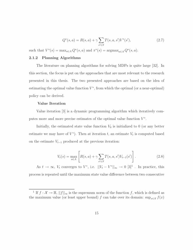
2.1.2 Planning Algorithms

The literature on planning algorithms for solving MDPs is quite large [32]. In

this section, the focus is put on the approaches that are most relevant to the research

presented in this thesis. The two presented approaches are based on the idea of

estimating the optimal value function V ∗, from which the optimal (or a near-optimal)

policy can be derived.

Value Iteration

Value iteration [3] is a dynamic programming algorithm which iteratively com-

putes more and more precise estimates of the optimal value function V ∗.

Initially, the estimated state value function V0 is initialized to 0 (or any better

estimate we may have of V ∗). Then at iteration t, an estimate Vt is computed based

on the estimate Vt−1 produced at the previous iteration:

Vt(s) = maxa∈A

[

R(s, a) + γ∑

s′∈ST (s, a, s′)Vt−1(s

′)

]

. (2.8)

As t → ∞, Vt converges to V ∗, i.e. ||Vt − V ∗||∞ → 0 [3]1 . In practice, this

process is repeated until the maximum state value difference between two consecutive

1 If f : X → R, ||f ||∞ is the supremum norm of the function f , which is defined asthe maximum value (or least upper bound) f can take over its domain: supx∈X f(x)

15

iterations is smaller than some threshold ε > 0 (i.e. until ||Vt − Vt−1||∞ < ε). Upon

completion of the algorithm, the policy derived from Vt is defined as:

πt+1(s) = argmaxa∈A

[

R(s, a) + γ∑

s′∈ST (s, a, s′)Vt(s

′)

]

. (2.9)

If ||Vt − Vt−1||∞ < ε, this guarantees that ||V ∗ − V πt+1||∞ < 2γε1−γ [81]. Hence

to guarantee that πt+1 is ε-optimal2 , one should proceed with value iteration until

||Vt − Vt−1||∞ < (1−γ)ε2γ

.

The complexity of one iteration of value iteration is O(|S|2|A|). To find an ε-

optimal policy, value iteration must proceed with O( log(||R||∞)+log(1/ε)+log(1/(1−γ))+11−γ )

iterations [49].

Sparse Sampling

One drawback of the value iteration algorithm is that it is very long to compute

when the set of states is large (as the complexity is quadratic in the number of

states). One solution to this problem proposed by Kearns et al. [47] is to use Monte

Carlo sampling methods to estimate the expected return obtained at future states

instead of computing the expectation exactly as in value iteration.

In this approach, an estimate Vt(s) of Vt(s) is computed as follows:

Vt(s) = maxa∈A

[

R(s, a) +γ

N

N∑

i=1

Vt−1(s′s,ai )

]

, (2.10)

2 A policy π is ε-optimal if ||V ∗ − V π||∞ < ε

16

where s′s,a1 , . . . , s′s,aN is a random sample from the distribution T (s, a, ·). At t = 0,

V0 = V0 = 0. This algorithm is usually computed online (i.e. during the execution

of the agent) only for the current state s of the agent. In this case, the algorithm

only tries to find the best action for the current state s. Hence, if the agent plans

for a horizon of t, Vt(s) is only computed for the current state s. Sampling a next

state from the distribution T (s, a, ·) can be achieved in O(log |S|), so doing a t-step

lookahead with N sampled next states at each action is in O((|A|N)t log |S|). Kearns

et al. also derive a bound on the depth t and the number of samples N required in

order to obtain an estimate Vt(s) within ε of V ∗(s) with high probability.

2.2 Partially Observable Markov Decision Processes

As mentioned previously, the POMDP generalizes the MDP to handle partially

observable domains in which the agent has uncertainty about its current state [71].

A POMDP is defined formally by seven components (S,A, Z, T, O,R, γ). As in the

MDP, S represents the set of states,A the set of actions, T : S × A× S → [0, 1] the

transition function, R : S × A → R the reward function and γ ∈ [0, 1) the discount

factor. The only difference here is the addition of Z and O:

• Observations: Z is the set of observations the agent can perceive in its envi-

ronment.

• Observation Probabilities: O : S × A × Z → [0, 1] is the observation

function, where O(s′, a, z) specifies the probability P (zt = z|st = s′, at−1 = a)

that the agent observes z when it moves to state s′ by doing action a. For any

fixed state s′ ∈ S and action a ∈ A, O(s′, a, ·) is a probability distribution over

observations z ∈ Z, so that∑

z∈Z O(s′, a, z) = 1. Again, it is assumed that the

17

observation probabilities are time-homogeneous and do not depend on previous

states (Markov assumption).

In a POMDP, the current state of the environment is a hidden variable, it is

not perceived by the agent. Instead, at each step, it perceives an observation z ∈ Z,

which depends on the unknown current state and previous action. Due to this

dependency, the observation z carries some information about the unknown current

state. However, because one observation can usually be observed in many different

states, it does not allow the agent to know exactly in which state it is.

2.2.1 Belief State and Value Function

Since the states are not observable, the agent cannot choose its actions based

on the states. It has to consider the uncertainty it has on its current state. Since the

current state depends on the previous state of the system, this uncertainty depends

on the uncertainty on the previous state, which in turn depends on the uncertainty

of the state before, and so on. Hence the uncertainty on the current state depends

on the complete history of past actions and observations. The history at time t is

defined as:

ht = {a0, z1, . . . , zt−1, at−1, zt}. (2.11)

This explicit representation of the past is typically memory expensive. Instead,

it is possible to summarize all relevant information from previous actions and ob-

servations in a probability distribution over the set of states S, which is called a

belief state [1]. The belief state bt at time t is defined as the posterior probability

18

distribution of being in each state, given the complete history:

bt(s) = Pr(st = s|ht, b0). (2.12)

It has been shown that the belief state bt is a sufficient statistic for the history

ht [68], therefore the agent can choose its actions based on the current belief state bt

instead of all past actions and observations. Initially, the agent starts with an initial

belief state b0, representing its knowledge about the starting state of the environment.

Then, at any time t, the belief state bt can be computed from the previous belief

state bt−1, using the previous action at−1 and the current observation zt. This is done

via the belief update function :

bt(s′) =

1

Pr(zt|bt−1, at−1)O(s′, at−1, zt)

∑

s∈ST (s, at−1, s

′)bt−1(s), (2.13)

where Pr(z|b, a), the probability of observing z after doing action a in belief b, acts

as a normalizing constant such that bt remains a probability distribution:

Pr(z|b, a) =∑

s′∈SO(s′, a, z)

∑

s∈ST (s, a, s′)b(s). (2.14)

We define bt = τ(bt−1, at−1, zt−1) to be the Bayes’ update rule from prior bt−1 to

posterior bt when observing zt after action at−1.

Now that the agent has a way of maintaining its uncertainty on the current

state, the next interesting question is how to determine the best action to take for

any particular belief the agent could hold.

19

Since the belief is a sufficient statistic of the complete history, the agent’s decision

only depends on the current belief rather than the complete history. Hence in a

POMDP, a policy π : ∆S × A→ [0, 1] is a mapping where for any belief b ∈ ∆S 3

and action a ∈ A, π(b, a) = P (at = a|bt = b) indicates the probability that the agent

performs action a in belief b. As in an MDP, the goal of the agent is to find a policy

π which maximizes its expected return over the infinite horizon. To achieve this, one

can proceed as in the MDP case, by defining a value function V π : ∆S → R that

specifies the expected return obtained by following the policy π starting in belief b.

Since the belief is a sufficient statistic of the past, transitions between belief

states satisfy the Markov assumption, so that the value function V π can be defined

by looking at the POMDP as an MDP (S ′, A′, T ′, R′) over belief states, called the

belief MDP. In the belief MDP, the set of states S ′ = ∆S corresponds to the set of

all beliefs of the POMDP, the set of actions A′ = A corresponds to the actions of

the original POMDP, the transition function T ′ specifies the probability of moving

from one belief to another by doing some action a, and the reward function R′

specifies the expected immediate reward obtained by doing action a in belief b, i.e.

R′(b, a) =∑

s∈S b(s)R(s, a). If the agent performs action a in belief b, then the

next belief depends on the observation z obtained by the agent. Hence there is a

probability Pr(z|b, a) of moving from belief b to belief τ(b, a, z) by doing action a.

It follows that T ′(b, a, b′) =∑

z∈Z I{b′}(τ(b, a, z)) Pr(z|b, a), where I{b′}(τ(b, a, z)) is

3 ∆S represents the space of probability distributions over the set S.

20

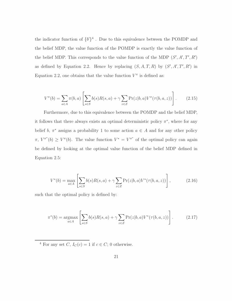
the indicator function of {b′}4 . Due to this equivalence between the POMDP and

the belief MDP, the value function of the POMDP is exactly the value function of

the belief MDP. This corresponds to the value function of the MDP (S ′, A′, T ′, R′)

as defined by Equation 2.2. Hence by replacing (S,A, T,R) by (S ′, A′, T ′, R′) in

Equation 2.2, one obtains that the value function V π is defined as:

V π(b) =∑

a∈Aπ(b, a)

[

∑

s∈Sb(s)R(s, a) + γ

∑

z∈ZPr(z|b, a)V π(τ(b, a, z))

]

. (2.15)

Furthermore, due to this equivalence between the POMDP and the belief MDP,

it follows that there always exists an optimal deterministic policy π∗, where for any

belief b, π∗ assigns a probability 1 to some action a ∈ A and for any other policy

π, V π∗(b) ≥ V π(b). The value function V ∗ = V π∗

of the optimal policy can again

be defined by looking at the optimal value function of the belief MDP defined in

Equation 2.5:

V ∗(b) = maxa∈A

[

∑

s∈Sb(s)R(s, a) + γ

∑

z∈ZPr(z|b, a)V ∗(τ(b, a, z))

]

, (2.16)

such that the optimal policy is defined by:

π∗(b) = argmaxa∈A

[

∑

s∈Sb(s)R(s, a) + γ

∑

z∈ZPr(z|b, a)V ∗(τ(b, a, z))

]

. (2.17)

4 For any set C, IC(c) = 1 if c ∈ C; 0 otherwise.

21

2.2.2 Planning Algorithms

There currently exists many algorithms to solve POMDPs. Most of the early

work focused on finding efficient algorithms that compute the value function V ∗ ex-

actly for some finite horizon t. We present some of these approaches below. However

due to the very large complexity of exact approaches, most of the recent work on

POMDP planners has focused on trying to find efficient approximate algorithms that

can compute V ∗ to a desired degree of accuracy. Many approximations have been

developed such as grid-based approximations [38, 6, 84, 4], finite-state automaton

policy representations [37, 52, 59, 8], point-based methods [57, 72, 69], and online

approximations [66, 78, 50, 55, 62]. The latter part of this section describes the

point-based and online methods, which are most relevant to the research in this

thesis.

Exact Approaches

A key result by Sondik [68] shows that the optimal value function for a finite-

horizon POMDP is piecewise-linear and convex. It means that the value function Vt

at any finite horizon t can be represented by a finite set of |S|-dimensional hyper-

planes: Γt = {α0, α1, . . . , αm}. These hyperplanes are often called α-vectors. Each

defines a linear value function over the belief state space associated with some action

a ∈ A. The value of a belief state is the maximum value returned by one of the α-

vectors for this belief state. The best action is the one associated with the α-vector

that returns the best value:

Vt(b) = maxα∈Γt

∑

s∈Sα(s)b(s). (2.18)

22

The Enumeration algorithm by Sondik [71] shows how the finite set of α-vectors

Γt can be built incrementally via dynamic programming. The idea is that any t-step

contingency plan can be expressed by an immediate action and a mapping associating

a (t-1)-step contingency plan to every observation the agent could get after this

immediate action. Hence if we know the value of these (t-1)-step contingency plan, we

can compute the value of the t-step contingency plan efficiently by reusing the values

computed for the (t-1)-step contingency plans. Initially, Sondik’s algorithm starts

by enumerating and computing the values of every 1-step plan, which corresponds

to all immediate action the agent could take. The value of these plans corresponds

directly to the immediate rewards:

Γa1 = {αa|αa(s) = R(s, a)},

Γ1 =⋃

a∈A Γa1.(2.19)

Then to build the α-vectors at time t, it looks at all possible immediate actions

the agent could take and every combination of (t-1)-step plans to pursue after the

observation made after the immediate actions. The value of these plans corresponds

to the immediate rewards obtained by the immediate action and the discounted

future expected value obtained by the (t-1)-step plans:

Γa,zt = {αa,zi |αa,zi (s) =

∑

s′∈S T (s, a, s′)O(s′, a, z)α′i(s

′), α′i ∈ Γt−1},

Γat = Γa1 ⊕ Γa,z1t ⊕ Γa,z2t ⊕ · · · ⊕ Γa,z|Z|

t ,

Γt =⋃

a∈A Γat ,

(2.20)

23

where ⊕ is the cross-sum operator5 .

Most of the work on exact POMDP approaches [71, 53, 12, 48, 10, 83] aims

to limit the growth of the set Γt by finding efficient ways to prune α-vectors that

are dominated, i.e. α-vectors that do not maximize the value function at any belief

state in Equation 2.18. Dominated α-vectors can be removed without affecting the

exactness of the value function as subsequent α-vectors generated at the next itera-

tion by these dominated α-vectors will also be dominated. Nevertheless, in general,

the number of α-vectors needed to represent the value function grows exponentially

in the number of observations at each iteration, i.e. the size of the set Γt is in

O(|A||Γt−1||Z|). Since each new α-vector requires computation time in O(|Z||S|2), the

resulting complexity of iteration t for exact approaches is in O(|A||Z||S|2|Γt−1||Z|).

Due to this large complexity, these methods have been limited to solve very small

problems (around 20 states and even fewer actions and observations) in practice.

Hence the need for efficient approximations that can scale to larger domains.

Point-Based Approaches

Point-based approaches [57, 72, 69] approximate the value function by updating

it only for some selected belief states. These point-based methods sample belief states

by simulating some random interactions of the agent with the POMDP environment,

and then updating the value function and its gradient over those sampled beliefs.

These approaches circumvent the complexity of exact approaches by sampling a small

set of beliefs and maintaining at most one α-vector per sampled belief state. Let B

5 Let A and B be sets of vectors, then A⊕B = {a+ b|a ∈ A, b ∈ B}.

24

represent the set of sampled beliefs, then the set Γt of α-vectors at time t is obtained

as follows:

αa(s) = R(s, a),

Γa,zt = {αa,zi |αa,zi (s) = γ

∑

s′∈S T (s, a, s′)O(s′, a, z)α′i(s

′), α′i ∈ Γt−1},

Γbt = {αab |αab = αa +

∑

z∈Z argmaxα∈Γa,zt

∑

s∈S α(s)b(s), a ∈ A},

Γt = {αb|αb = argmaxα∈Γbt

∑

s∈S b(s)α(s), b ∈ B}.

(2.21)

One can ensure that this yields a lower bound on V ∗ by initializing Γ0 with

a single α-vector α0(s) =mins′∈S,a∈AR(s′,a)

1−γ . Since |Γt−1| ≤ |B|, each iteration has

a complexity in O(|A||Z||S||B|(|S|+ |B|)), which is polynomial time, compared to

exponential time for exact approaches.

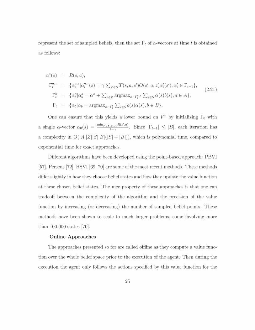
Different algorithms have been developed using the point-based approach: PBVI

[57], Perseus [72], HSVI [69, 70] are some of the most recent methods. These methods

differ slightly in how they choose belief states and how they update the value function

at these chosen belief states. The nice property of these approaches is that one can

tradeoff between the complexity of the algorithm and the precision of the value

function by increasing (or decreasing) the number of sampled belief points. These

methods have been shown to scale to much larger problems, some involving more

than 100,000 states [70].

Online Approaches

The approaches presented so for are called offline as they compute a value func-

tion over the whole belief space prior to the execution of the agent. Then during the

execution the agent only follows the actions specified by this value function for the

25

beliefs it encounters. Such approaches tend to be applicable only when dealing with

moderate-sized domains, since the policy construction step takes significant time and

does not scale well to large problems involving millions of states or hundreds of ob-

servations. In large POMDPs, a potentially better alternative is to use an online

approach [66, 78, 55, 50, 62], which only tries to find a good local policy for the

current belief state of the agent during the execution. The advantage of such an

approach is that it only needs to consider belief states that are reachable from the

current belief state within a limited planning horizon. This focuses computation on a

small set of beliefs. In addition, since online planning is done at every step (and thus

generalization between beliefs is not required), it is sufficient to calculate only the

maximal value for the current belief state, not the full α-vector. In this setting, the

policy construction steps and the execution steps are interleaved with one another.

An online algorithm takes as input the current belief state and returns the

single best action for this particular belief state. This is usually achieved by two

simple steps. First, the algorithm builds a tree of reachable belief states from the

current belief state. The current belief is the top node in this tree. Subsequent belief

states (as calculated by the τ(b, a, z) function of Equation 2.13) are represented

using OR-nodes (at which we must choose an action) and actions are included in

between each layer of belief nodes using AND-nodes (at which we must consider all

possible observations). Once the tree of reachable beliefs is built, the value of the

current belief is estimated by propagating value estimates up from the fringe nodes,

to their ancestors, all the way to the root, according to Bellman’s equation (Equation

2.16). An approximate value function is generally used at the fringe of the tree to

26

b0[14.4, 18.7]

a1

b2b1

z1 z2

a2

b4b3

z1 z2

1 3

0.7 0.3 0.5 0.5

a1

b6b5

z1 z2

a2

b8b7

z1 z2

-14

0.6 0.4 0.2 0.8

[14.4, 17.9] [12, 18.7]

[10, 18][9, 15][15, 20]

[6, 14] [9, 12][11, 20]

[10, 12]

[13.7, 16.9]

[5.8, 11.5]

[13.7, 16.9]

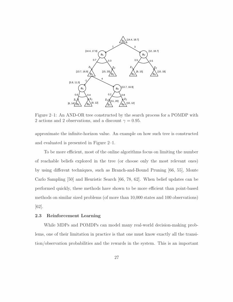
Figure 2–1: An AND-OR tree constructed by the search process for a POMDP with2 actions and 2 observations, and a discount γ = 0.95.

approximate the infinite-horizon value. An example on how such tree is constructed

and evaluated is presented in Figure 2–1.

To be more efficient, most of the online algorithms focus on limiting the number

of reachable beliefs explored in the tree (or choose only the most relevant ones)

by using different techniques, such as Branch-and-Bound Pruning [66, 55], Monte

Carlo Sampling [50] and Heuristic Search [66, 78, 62]. When belief updates can be

performed quickly, these methods have shown to be more efficient than point-based

methods on similar sized problems (of more than 10,000 states and 100 observations)

[62].

2.3 Reinforcement Learning

While MDPs and POMDPs can model many real-world decision-making prob-

lems, one of their limitation in practice is that one must know exactly all the transi-

tion/observation probabilities and the rewards in the system. This is an important

27

problem as usually these probabilities are not known exactly (only approximately

at best). In such case, if we simply provide an approximate model to the planning

algorithm, we may obtain a policy which is significantly different than the optimal

policy for the exact model. Hence, it becomes necessary to use learning algorithms

to improve the performance of the agent over time as it gathers more and more

experience in the system.

Reinforcement Learning (RL) [75] is a general framework that allows an agent,

starting with no knowledge of the system, to learn how to optimally achieve its task.

Most of the work on reinforcement learning has focused on the MDP case, where the

transition probabilities and rewards are completely unknown. In this setting, the

agent observes its current state and its immediate reward at every step. Under some

conditions, RL algorithms allow the agent’s behavior to converge toward the optimal

policy π∗ as its history of states, actions and rewards grows larger. RL algorithms

are usually defined by two components. One component tries to estimate the optimal

value function or optimal policy based on previous experience, and the second com-

ponent specifies the behavior of the agent, based on its optimal policy/value function

estimate and its exploration strategy. Estimating the optimal policy can be achieved

using model-free methods or model-based methods [75]. Model-free methods try

to learn the optimal policy directly, without learning the transition and immedi-

ate reward model, while model-based methods try to estimate the transition and

immediate reward model, in order to compute the optimal policy afterwards. We

first present these two types of methods and then present in more details different

exploration stategies that have been proposed in the literature.

28

2.3.1 Model-free methods

In order to learn directly the optimal policy, without learning the MDP model,

model-free methods usually try to directly estimate the state-action value function

Q∗ from the rewards and state transitions observed. One of the most popular method

of this type is the Q-Learning algorithm [79]. Q-Learning starts with an estimate

of the state-action value function Q. Q(s, a) can be initialized to 0 or to any better

estimate we may have. Then whenever the agent is in state s, performs action a,

observes reward r and moves to state s′, the estimate Q(s, a) is updated as follows:

Q(s, a) = Q(s, a) + α(r + γmaxa′∈A

Q(s′, a′)− Q(s, a)), (2.22)

where α ∈ (0, 1) is the learning rate. This equation can be thought of a gradient

descent update [18] of Q toward Q∗. Here r+ γmaxa′∈A Q(s′, a′) represents the new

estimate of Q∗(s, a) and Q(s, a) the old estimate. The update is performed with

proportion α of the difference between the new and old estimates, in the direction of

the new estimate.

The learning rate α is usually decreased over time such that α → 0 as the

estimate Q(s, a) converges. It has been shown that under some conditions on the

way α is decreased, and provided that every state and action is visited infinitely

often, then Q converges to Q∗ [79].

2.3.2 Model-based methods

Model-based methods explicitly learn the MDP parameters in order to derive the

optimal policy π∗. First, the transition probabilities T (s, a, s′) can be estimated by

looking at the observed frequency of such transitions in the history of the agent. Let

29

Nt(s, a, s′) =

∑t−1i=0 I{(s,a,s′)}(si, ai, si+1) represent the number of times a transition

from state s to state s′ occured by doing action a in the history of the agent at

time t, and Nt(s, a) =∑t−1

i=0 I{(s,a)}(si, ai) represent the number of times action a

was performed in state s in the history of the agent at time t. Then at time t,

the estimate Tt(s, a, s′) = Nt(s,a,s′)

Nt(s,a)is the maximum likelihood estimator (MLE) of

the exact transition probability T (s, a, s′). Furthermore, the rewards R(s, a) can

be estimated by looking at the average reward obtained by doing action a in s in

the history of the agent. Hence Rt(s, a) =∑ti=0 riI{(s,a)}(si,ai)

Nt(s,a)is the MLE of R(s, a)

at time t. Provided every state-action pair is visited infinitely often, the strong

law of large numbers guarantees that Tt(s, a, s′) → T (s, a, s′) almost surely and

Rt(s, a)→ R(s, a) almost surely as t→∞. Hence if the state-action value function

Q∗ is estimated by solving Qt(s, a) = Rt(s, a) + γ∑

s′∈S Tt(s, a, s′) maxa′∈A Qt(s

′, a′)

at time t, then we have that Qt → Q∗ almost surely as t → ∞. Consequently, the

optimal policy πt estimated for Qt, i.e. πt(s) = argmaxa∈A Qt(s, a), converges to π∗.

2.3.3 Exploration

Now that the agent has a way to learn the optimal policy, the last remaining

problem is how the agent should select its action at any time t based on its current

estimate Q. As mentionned in the introduction, one problem that arises is the need

to balance exploration and exploitation. If too little exploration is performed, the

agent might not learn a good estimate Q(s, a) for some state-action pairs. This may

lead it to follow a sub-optimal policy. On the other hand, exploration is usually

risky and can have very high cost, so that, if the agent explores too much, then the

learning phase may prove very costly.

30

The problem of balancing exploration and exploitation has been studied greatly

in bandit problems [31]. Such problems correspond to 1-state MDPs with multiple

actions where each action has a different distribution over immediate rewards. Gittins

[31] derived an optimal solution for these problems which can be computed efficiently.

Each action is associated to a Gittins index and the optimal policy is simply to

execute the action with highest Gittins index at any time t. However this optimal

policy relies on the fact that there is only 1-state and does not extend to general

MDPs.

In RL, most work on exploration has focused on developing different heuristics to

balance the exploration and exploitation. We now present some of these techniques

below.

ε-greedy and Boltzmann exploration

ε-greedy and Boltzmann exploration are two very simple and well known explo-

ration strategies. Under the ε-greedy strategy, at any step t, the agent performs a

uniformly random action a ∈ A with probability ε > 0, and with probability 1 − ε,

performs the greedy action argmaxa∈A Q(s, a) that seems best for the current state

s under the current estimate state-action value function Q.

Boltzmann exploration is a more efficient exploration strategy which tries to

bias the exploration towards action that have the highest value estimates. This lim-

its further exploration of actions which are known to be bad from past experience,

and thus improves the sum of rewards gathered by the agent during learning. Given

current state s and estimate Q, the Boltzmann exploration strategy is to perform

31

action a ∈ A with probability P (a|s) ∝ exp(Q(s, a)/∆), where ∆ > 0 is a tempera-

ture parameter that allows to control the amount of exploration. As ∆→∞, P (a|s)

tends to a uniform distribution so that the agent always explores, while as ∆ → 0,

P (a|s)→ 1 for a = argmaxa′∈A Q(s, a′) so that the agent always performs the greedy

action.

Since in both methods, the agent can choose any action with some probability

greater than 0, this ensures that each state and action will be visited infinitely often,

so that the convergence property of Q to Q∗ holds. However in practice, ε and

∆ strongly influences the performance and must be fine-tuned to produce the best

results. Furthermore, ε and ∆ are usually decreased over time so that in the limit,

the agent always behave optimally.

One problem with both of these methods is that the exploration occurs randomly

and is not focused on what needs to be learned. For instance, both methods could

take exploration action that lead to states which have already been visited very often,

and that will not improve the estimate Q. Another problem is that ε-greedy does

not consider the cost of the exploratory actions, which can hinder significantly the

rewards obtained by the agent during the learning phase.

Interval Estimation

Interval Estimation [43] and Model-based Interval Estimation methods [80, 74,

73] compute confidence intervals [L(s, a);U(s, a)] on the state-action values Q∗(s, a),

such that based on the history of state transitions and rewards of the agent, Q∗(s, a) ∈

[L(s, a);U(s, a)] with high probability. Then at any time t in state s, the agent

executes the action a with highest upper bound, i.e. a = argmaxa′∈A U(s, a′). Since

32

actions which haven’t been tried often before (or that can lead to areas of the state

space which haven’t been visited often) have large confidence intervals and actions

that have been tried often (and lead to states that have been visited often) have small

confidence intervals, this technique favors the exploration of actions that haven’t been

tried often before or that lead to states that haven’t been visited often. Furthermore,

it also takes into account the previous rewards obtained by the actions in order to

prevent exploration of actions that are known to be bad.

Strehl et al. [73] derived strong polynomial-time bound on the number of steps

required by the agent to perform near-optimally with high probability when using

the Model-based Interval Estimation exploration strategy.

E3 Algorithm

The E3 algorithm (Explicit Explore or Exploit) [46] splits the state space S

into known and unknown states. Whenever the agent is in an unknown state, it

always explores such as to improve its knowledge of the MDP, while when the agent

is in a known state, it always exploits its current knowledge by choosing the greedy

action which maximize its rewards. At the begining, all states are unknown. A

state becomes known whenever the agent has visited it a sufficient number of times

M . Kearns et al. derived a polynomial bound on M in order to guarantee that the

estimate Q for known states is sufficiently close to Q∗, so that the greedy actions are

near-optimal with high probability.

R-MAX

The R-MAX algorithm [7] is a simpler generalization of E3. R-MAX creates a

virtual absorbing state s0 where every state s ∈ S which hasn’t been visited at least

33

M times transits to it determiniscally. In s0 the agent always obtains the maximum

reward Rmax = maxs∈S,a∈AR(s, a). When a state has been visited M times, the

transition probabilities for that state are changed to the estimated probabilities from

the M samples. With this model, the agent always executes the action with highest

expected long-term rewards. Since every state which has been visited less than M

times transits to s0 and obtains Rmax rewards at every following steps, actions that

lead to such states will always have very high values, thus favoring the exploration

of these states, until they have been visited M times. M can be defined as in the E3

algorithm in order to guarantee convergence to a near-optimal behavior with high

probability in polynomial time.

2.3.4 Reinforcement Learning in POMDPs

Reinforcement Learning in POMDPs has received little attention in the AI com-

munity so far. One of the main difficulty with RL in POMDPs is that one needs to

know the model to maintain the belief state of the agent. If only an approximate

model is used, then the belief state may diverge significantly from the correct be-

lief state maintained with the exact model, so that the learning will not function

properly.

For this reason, RL methods in POMDPs [24] typically use history-based rep-

resentations of the belief and learn a Q-value function based on these histories. One

difficulty that arises is the following: unless one has a means of returning to the

initial belief state, a particular history can only be visited once, and it would be

impossible to visit all possible histories. To solve this problem, Even-Dar et al. [24]

34

show that in any connected POMDP6 , there exists a homing strategy (random walk)

that returns approximately to the initial belief. By repeatedly using such homing

strategy, the agent can learn about the value of each action in every history for some

finite horizon t. Such an approach remains fairly theoretical and does not work well

in practice as the agent may get very bad rewards during the homing sequence.

A more practical approach called Utile Suffix Memory [51] learns a decision-

tree based on the short-term memory of the agent (i.e. the last few actions and

observations in the history of the agent). In this tree, each path from the root

to a fringe node represents a short-term memory of the agent starting from the

current belief, going backward in time. At each fringe node, a Q-value is learned for

each action, representing the value of performing that action after that short-term

memory. Then if the distribution in Q-values is deemed significantly different (via

a Kolmogorov-Smirnov test) when looking 1-step further in the short-term memory

of the agent, then the fringe node is expanded to further distinguish between these

histories. Initially, the tree contains only one root node and is grown by following

this procedure. In the end, the tree represents the short-term memories that lead to

significantly different future rewards and that must be distinguished to perform well.

6 A connected POMDP is a POMDP such that from any state s, the agent canreach any other state s′ with non-zero probability by doing some sequence of actions.

35

CHAPTER 3

Model-Based Bayesian Reinforcement Learning: Related Work

Bayesian Reinforcement Learning (BRL) is a new Reinforcement Learning frame-

work which seeks to address the exploration-exploitation trade-off problem [20]. The

main idea behind model-based BRL is to explicitly represent the uncertainty on the

model learned by the agent via bayesian learning approaches. This in turn allows us

to cast the exploration-exploitation problem as a decision problem, where the agent

seeks to maximize its expected return with respect to the uncertainty on its model

and how this uncertainty evolves over time.

As a side note, model-free BRL methods also exist [22, 23, 30, 29]. Instead

of representing the uncertainty on the model, these methods explitcitly model the

uncertainty on the value function or policy. However, these methods do not guaran-

tee an optimal exploration-exploitation tradeoff and still have to rely on heuristics

to handle this trade-off. Furthermore, in practice it is often easier to express prior

knowledge (initial uncertainty) on the model than on the value function. For ex-

ample, sensors and actuators used in robotics and other manufacturing applications

will usually have confidence interval on their accuracy and failure rate provided by

the manufacturer, so that appropriate priors that assigns most of the probability

mass over the given confidence interval can be defined. Further discussion on how

to choose the prior in practice is provided below. This thesis focuses entirely on

36

model-based BRL methods, so that we restrict our survey to these methods in this

chapter.

This chapter first presents the general principles of bayesian learning, and then

reviews some of the related work on model-based BRL in MDPs.

3.1 Bayesian Learning

Bayesian Learning (or Bayesian Inference) is a general technique for learning

the unknown parameters of a probability model from observations generated by this

model [9]. In bayesian learning, a probability distribution is maintained over all pos-

sible values of the unknown parameters. As observations are made, this probability

distribution is updated via Bayes’ rule, and probability density increases around the

most likely parameter values.

Formally, consider a random variable X with probability distribution fX|Θ over

its domain X parameterized by the unknown vector of parameters Θ in some pa-

rameter space P. Let X1, X2, · · · , Xn be an independent random sample from fX|Θ.

Then by Bayes’ rule, the posterior probability density gΘ|X1,X2,...,Xn(θ|x1, x2, . . . , xn)

of the parameters Θ = θ, after the observations of X1 = x1, X2 = x2, · · · , Xn = xn,

is:

gΘ|X1,X2,...,Xn(θ|x1, x2, . . . , xn) =gΘ(θ)

∏ni=1 fX|Θ(xi|θ)

∫

P gΘ(θ′)∏n

i=1 fX|Θ(xi|θ′)dθ′, (3.1)

where gΘ(θ) is the prior probability density of Θ = θ, i.e. gΘ over the parameter

space P is a distribution that represents the initial belief (or uncertainty) on the

values of Θ. Note that the posterior can be defined recursively as follows:

37

gΘ|X1,X2,...,Xn(θ|x1, x2, . . . , xn) =gΘ|X1,X2,...,Xn−1(θ|x1, x2, . . . , xn−1)fX|Θ(xn|θ)

∫

P gΘ|X1,X2,...,Xn−1(θ′|x1, x2, . . . , xn−1)fX|Θ(xn|θ′)dθ′

,

(3.2)

so that whenever we get the nth observation of X, xn, we can compute the new

posterior distribution gΘ|X1,X2,...,Xn from the previous posterior gΘ|X1,X2,...,Xn−1.

3.1.1 Conjugate Families

In general, updating the posterior distribution gΘ|X1,X2,...,Xn is difficult due to

the need to compute the normalization constant∫

P gΘ(θ)∏n

i=1 fX|Θ(xi|θ)dθ. How-

ever, for conjugate familiy distributions, updating the posterior can be achieved very

efficiently with a simple update of the parameters defining the posterior distribution

[9].

Formally, consider a particular class G of prior distributions over the parameter

space P, and a class F of likelihood functions fX|Θ over X parameterized by param-

eters Θ ∈ P, then F and G are said to be conjugate if for any choice of prior gΘ ∈ G,

likelihood fX|Θ ∈ F and observation X = x, the posterior distribution gΘ|X after

observation of X = x is also in G.

For example, the Beta distribution1 is conjugate to the Binomial distribution2 .

Consider X ∼ Binomial(n, p) with unknown probability parameter p, and consider

1 Beta(α, β) is defined by the density function f(p|α, β) ∝ pα−1(1 − p)β−1 forp ∈ [0, 1] and parameters α, β ≥ 0

2 Binomial(n, p) is defined by the density function f(k|n, p) ∝ pk(1 − p)n−k fork ∈ {0, 1, . . . , n} and parameters p ∈ [0, 1],n ∈ N

38

a prior Beta(α, β) over the unknown value of p. Then after the observation ofX = x,

the posterior over p is also Beta distributed and is defined by Beta(α+x, β+n−x).

3.1.2 Choice of Prior

One important issue with bayesian methods is the need to specify a prior. While

the influence of the prior tends to be negligible when provided with a large amount

of data, its choice is particularly important for any inference and decision-making

performed when only a small amount of data has been observed.

In general, the prior should reflect any knowledge of the model available a pri-

ori. In many practical problems, informative priors can be obtained. As mentioned

before, often sensors and actuators used in many engineering applications will have

specified confidence intervals on their accuracy provided by the manufacturer so that

informative priors on the parameters describing these components can be defined to

fit these confidence intervals. In many other applications, such as medical treatment

design or portfolio management, data about the problem may have already been col-

lected by specialists in the field, so that this data can be used to define an informative

prior over the parameter space. In the absence of such data, one could construct an

informative prior by gathering a small set of observations, e.g. by executing a random

policy, and then using these observations to construct an informative prior.

In the absence of any knowledge, uninformative priors can be specified. Un-

der such priors, any inference done a posteriori is dominated by the data, i.e. the

influence of the prior is minimal. A typical uninformative prior is to use a prior

distribution which is constant over the whole parameter space Θ, such that every

possible parameter has equal probability density. From an information theoretic

39

point of view, such priors have maximum entropy and thus contain the least amount

of information about θ [40]. However, one problem with such uniform priors is that

if φ = t(θ) is a 1-1 transformation of θ used to reparametrize the probability model

fX|Θ, then the prior for φ, obtained from a uniform prior over Θ, may not be uni-

form. Hence under different reparametrization, one would have different amounts of

information about the unknown parameter, which can be somewhat unsatisfactory.

A prefered uninformative prior, which is invariant under reparametrization, is

Jeffreys’ prior [41]. It is defined to be proportional to the square root of the absolute

value of the determinant of the Fisher Information matrix3 :

gΘ(θ) ∝ |I(θ)|12 (3.3)

As mentioned, Jeffreys’ prior is invariant under reparametrization, that is, if

φ = t(θ) is a 1-1 transformation of θ, then the prior for φ, obtained from Jeffreys’ prior

over Θ, is precisely Jeffreys’ prior for φ. This property implies that reparametrizing

the probability model under a 1-1 transformation gives us no information.

In the previous example of learning the parameter p of a Binomial(n, p) distri-

bution, Jeffreys’ prior corresponds to the Beta(12, 1

2) distribution. This turns out to

be different than the uniform distribution over [0, 1] (i.e. Beta(1, 1)). The reader is

3 Consider θ ∈ Θ to be a parameter vector with n elements for the probabilitymodel fX|Θ, then the Fisher Information matrix I(θ) is a n × n matrix such that

element Iij(θ) = −E[

∂∂θi

∂∂θj

ln fX|Θ(X|θ)]

, where the expectation is taken over X

with distribution fX|Θ(·|θ).

40

refered to Kass & Wasserman’s survey of formal methods for choosing uninformative

priors [45] for a more in depth discussion on this subject.

3.1.3 Convergence

Another important issue with bayesian methods concerns the convergence of

the posterior towards the true parameter of the system. Since a prior must be

specified, one may be concerned about whether the posterior probability density will

be concentrated around the true parameter, no matter which prior is used, and how

fast will the posterior converge given the specified prior.

In general, the posterior density concentrates around the parameters that have

highest likelihood of generating the observed data in the limit. For finite param-

eter spaces, and for smooth families with continuous finite dimensional parameter

spaces, the posterior converges towards the true parameter as long as the prior as-

signs non-zero probability to every neighborhood of the true parameter. If the prior

assigns zero probability density to the true parameter then the posterior will con-

centrate around the most likely parameters that have non-zero prior density. Hence

in practice it is often desirable to assign non-zero prior density over the whole pa-

rameter space. However even though non-zero prior density may be assigned to the

true parameters, some convergence problems may arise when the parameter space is

infinite dimensional, e.g. when using non-parametric methods. Freedman [27] gave

some examples of such problems. However, under some conditions on the prior [67],

one can still guarantee that the posterior will converge to the correct parameters in

the infinite dimensional case. See Doob [16] and Schwartz [67] for a more in depth

discussions on these issues.

41

It should also be noted that if multiple parameters within the parameter space

can generate the observed data with equal likelihood, then the posterior distribution

will usually be multimodal, with one mode surrounding each equally likely parameter.

In such case it is impossible to identify the true underlying parameter. However

for practical purposes, such as making predictions about future observations, it is

sufficient to identify any of the equally likely parameters.

Finally, another concern is how fast the posterior converges towards the true

parameters. This is mostly influenced by how far the prior is from the true parameter.

If the prior is poor, i.e. it assigns most probability density to parameters far from

the true parameters, then it will take much more data to learn the correct parameter

than if the prior assigns most probability density around the true parameter. For

such reasons, a safe choice is to start with an uninformative prior, unless some data

is already available for this problem.

3.2 Bayesian Reinforcement Learning in Markov Decision Processes

Model-based Bayesian Reinforcement Learning in MDPs has received more at-

tention from the AI community lately as it provides an optimal solution to the

exploration-exploitation trade-off in standard Reinforcement Learning [20], given a

specified prior distribution on the model. Hence, in many applications where gath-

ering data for learning is expensive, these methods allow for efficient exploration

and learning of the task domain while minimizing costs. Furthermore, it provides

a framework for planning under uncertainty in the model parameters, which often

occurs in practice. Note that in standard reinforcement learning, a prior on the

model parameters is not usually specified. In such case, Jeffreys’ prior (see Section

42

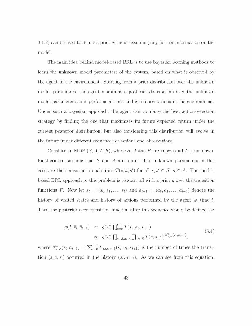
3.1.2) can be used to define a prior without assuming any further information on the

model.

The main idea behind model-based BRL is to use bayesian learning methods to

learn the unknown model parameters of the system, based on what is observed by

the agent in the environment. Starting from a prior distribution over the unknown

model parameters, the agent maintains a posterior distribution over the unknown

model parameters as it performs actions and gets observations in the environment.

Under such a bayesian approach, the agent can compute the best action-selection

strategy by finding the one that maximizes its future expected return under the

current posterior distribution, but also considering this distribution will evolve in

the future under different sequences of actions and observations.

Consider an MDP (S,A, T,R), where S, A and R are known and T is unknown.

Furthermore, assume that S and A are finite. The unknown parameters in this

case are the transition probabilities T (s, a, s′) for all s, s′ ∈ S, a ∈ A. The model-

based BRL approach to this problem is to start off with a prior g over the transition

functions T . Now let st = (s0, s1, . . . , st) and at−1 = (a0, a1, . . . , at−1) denote the

history of visited states and history of actions performed by the agent at time t.

Then the posterior over transition function after this sequence would be defined as:

g(T |st, at−1) ∝ g(T )∏t−1i=0 T (si, ai, si+1)

∝ g(T )∏

s∈S,a∈A∏

s′∈S T (s, a, s′)Nas,s′

(st,at−1),(3.4)

where Nas,s′(st, at−1) =

∑t−1i=0 I{(s,a,s′)}(si, ai, si+1) is the number of times the transi-

tion (s, a, s′) occurred in the history (st, at−1). As we can see from this equation,

43

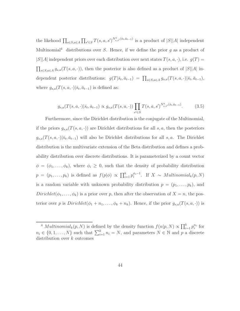
the likehood∏

s∈S,a∈A∏

s′∈S T (s, a, s′)Nas,s′

(st,at−1) is a product of |S||A| independent

Multinomial4 distributions over S. Hence, if we define the prior g as a product of

|S||A| independent priors over each distribution over next states T (s, a, ·), i.e. g(T ) =

∏

s∈S,a∈A gs,a(T (s, a, ·)), then the posterior is also defined as a product of |S||A| in-

dependent posterior distributions: g(T |st, at−1) =∏

s∈S,a∈A gs,a(T (s, a, ·)|st, at−1),

where gs,a(T (s, a, ·)|st, at−1) is defined as:

gs,a(T (s, a, ·)|st, at−1) ∝ gs,a(T (s, a, ·))∏

s′∈ST (s, a, s′)N

as,s′

(st,at−1). (3.5)

Furthermore, since the Dirichlet distribution is the conjugate of the Multinomial,

if the priors gs,a(T (s, a, ·)) are Dirichlet distributions for all s, a, then the posteriors

gs,a(T (s, a, ·)|st, at−1) will also be Dirichlet distributions for all s, a. The Dirichlet

distribution is the multivariate extension of the Beta distribution and defines a prob-

ability distribution over discrete distributions. It is parameterized by a count vector

φ = (φ1, . . . , φk), where φi ≥ 0, such that the density of probability distribution

p = (p1, . . . , pk) is defined as f(p|φ) ∝∏k

i=1 pφi−1i . If X ∼ Multinomialk(p,N)

is a random variable with unknown probability distribution p = (p1, . . . , pk), and

Dirichlet(φ1, . . . , φk) is a prior over p, then after the observation of X = n, the pos-

terior over p is Dirichlet(φ1 + n1, . . . , φk + nk). Hence, if the prior gs,a(T (s, a, ·)) is

4 Multinomialk(p,N) is defined by the density function f(n|p,N) ∝∏k

i=1 pnii for

ni ∈ {0, 1, . . . , N} such that∑k

i=1 ni = N , and parameters N ∈ N and p a discretedistribution over k outcomes

44

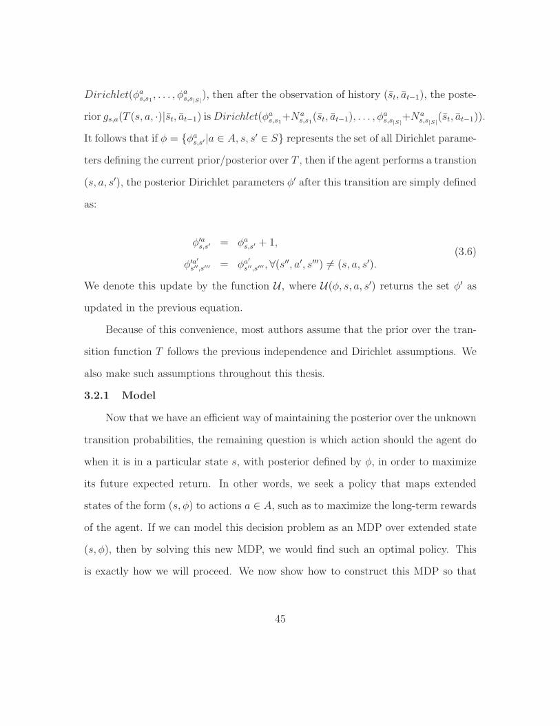
Dirichlet(φas,s1, . . . , φas,s|S|

), then after the observation of history (st, at−1), the poste-

rior gs,a(T (s, a, ·)|st, at−1) isDirichlet(φas,s1+Nas,s1(st, at−1), . . . , φ

as,s|S|

+Nas,s|S|

(st, at−1)).

It follows that if φ = {φas,s′|a ∈ A, s, s′ ∈ S} represents the set of all Dirichlet parame-

ters defining the current prior/posterior over T , then if the agent performs a transtion

(s, a, s′), the posterior Dirichlet parameters φ′ after this transition are simply defined

as:

φ′as,s′ = φas,s′ + 1,

φ′a′s′′,s′′′ = φa

′

s′′,s′′′, ∀(s′′, a′, s′′′) 6= (s, a, s′).

(3.6)

We denote this update by the function U , where U(φ, s, a, s′) returns the set φ′ as

updated in the previous equation.

Because of this convenience, most authors assume that the prior over the tran-

sition function T follows the previous independence and Dirichlet assumptions. We

also make such assumptions throughout this thesis.

3.2.1 Model

Now that we have an efficient way of maintaining the posterior over the unknown

transition probabilities, the remaining question is which action should the agent do

when it is in a particular state s, with posterior defined by φ, in order to maximize

its future expected return. In other words, we seek a policy that maps extended

states of the form (s, φ) to actions a ∈ A, such as to maximize the long-term rewards

of the agent. If we can model this decision problem as an MDP over extended state

(s, φ), then by solving this new MDP, we would find such an optimal policy. This

is exactly how we will proceed. We now show how to construct this MDP so that

45

the optimal solution will be the optimal exploration-exploitation trade-off under the

current prior/posterior.

Let’s define this new MDP by the tuple (S ′, A′, T ′, R′). As we just mentionned,

since we want the agent to find the best action a ∈ A to perform in any ex-

tended state (s, φ), we define the new set of state S ′ = S × T , where T = {φ ∈

N|S|2|A||∀(s, a) ∈ S × A,

∑

s′∈S φass′ > 0}, and A′ = A. Here, the constraints on

the set T of possible count parameters φ are only to ensure the transition prob-

abilities, as defined below, are well defined. To avoid confusion we refer to the

extended states (s, φ) ∈ S ′ as hyperstates. Also note that the next information

state φ′ only depends on the previous information state φ and the transition (s, a, s′)

that occurs in the physical system, so that transitions between hyperstates also ex-

hibit the Markov property. Since we want the agent to maximize the rewards it

obtains in the physical system, the reward function R′ should return the same re-

wards that the agent obtains in the physical system, as defined in R. Thus we

define R′(s, φ, a) = R(s, a). It remains only to define the transition probabilities be-

tween hyperstates. The new transition function T ′ must specify the transition prob-

abilities T ′(s, φ, a, s′, φ′) = Pr(s′, φ′|s, a, φ). By the chain rule, Pr(s′, φ′|s, a, φ) =

Pr(s′|s, a, φ) Pr(φ′|s, a, s′, φ). Since the update of the information state φ to φ′ is

deterministic, then Pr(φ′|s, a, s′, φ) is either 0 or 1, depending on whether φ′ =

U(φ, s, a, s′) or not. Hence Pr(φ′|s, a, s′, φ) = I{φ′}(U(φ, s, a, s′)). By the law of to-

tal probability, Pr(s′|s, a, φ) =∫

Pr(s′|s, a, T, φ)f(T |φ)dT =∫

T (s, a, s′)f(T |φ)dT ,

where the integral is caried over transition function T , and f(T |φ) is the proba-

bility density of transition function T under the posterior defined by φ. The term

46

∫

T (s, a, s′)f(T |φ)dT is the expectation of T (s, a, s′) for the Dirichlet posterior de-

fined by the parameters φas,s1, . . . , φas,s|S|

, which corresponds toφas,s′

∑

s′′∈S φas,s′′

. Thus it

follows that T ′(s, φ, a, s′, φ′) =φas,s′

∑

s′′∈S φas,s′′

I{φ′}(U(φ, s, a, s′)).

Hence we now have a new MDP with a known model that represents the

exploration-exploitation trade-off problem. By solving this MDP, we can find the

optimal exploration-exploitation strategy to follow, given any prior knowledge we

may have on the environment. This new MDP is often called Bayes-Adaptive MDP

[20] or HyperMDP [11].

Notice that while we have assumed that the reward function R is known, this

BRL framework can easily be extended to the case where R is unknown. In such case,

one can proceed similarly by using a bayesian learning method to learn the reward

function R and add the posterior parameters for R in the hyperstate. The new

reward function R′ then becomes the expected reward under the current posterior

over R, and the transition function T ′ would also model how to update the posterior

over R, upon the observation of any reward r. For brevity of presentation, it is

always assumed that the reward function is known in the remainder of this thesis.

However, the frameworks we present in the following sections can be easily extended

to handle cases where the rewards are unknown, by following a similar reasoning.

3.2.2 Optimality and Value Function

The Bayes-Adaptive MDP (BAMDP) is just an MDP with a countably infinite

number of states. It follows that all the theoretical results derived for MDPs carries

to Bayes-Adaptive MDPs. Hence, we know there exists an optimal deterministic

policy π∗ : S ′ → A, and that its value function is defined by:

47

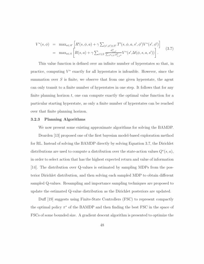
V ∗(s, φ) = maxa∈A′

[

R′(s, φ, a) + γ∑

(s′,φ′)∈S′ T ′(s, φ, a, s′, φ′)V ∗(s′, φ′)]

= maxa∈A

[

R(s, a) + γ∑

s′∈Sφas,s′

∑

s′′∈S φas,s′′

V ∗(s′,U(φ, s, a, s′))

]

.(3.7)

This value function is defined over an infinite number of hyperstates so that, in

practice, computing V ∗ exactly for all hyperstates is infeasible. However, since the

summation over S is finite, we observe that from one given hyperstate, the agent

can only transit to a finite number of hyperstates in one step. It follows that for any

finite planning horizon t, one can compute exactly the optimal value function for a

particular starting hyperstate, as only a finite number of hyperstates can be reached

over that finite planning horizon.

3.2.3 Planning Algorithms

We now present some existing approximate algorithms for solving the BAMDP.

Dearden [13] proposed one of the first bayesian model-based exploration method

for RL. Instead of solving the BAMDP directly by solving Equation 3.7, the Dirichlet

distributions are used to compute a distribution over the state-action values Q∗(s, a),

in order to select action that has the highest expected return and value of information

[14]. The distribution over Q-values is estimated by sampling MDPs from the pos-

terior Dirichlet distribution, and then solving each sampled MDP to obtain different

sampled Q-values. Resampling and importance sampling techniques are proposed to

update the estimated Q-value distribution as the Dirichlet posteriors are updated.

Duff [19] suggests using Finite-State Controllers (FSC) to represent compactly

the optimal policy π∗ of the BAMDP and then finding the best FSC in the space of

FSCs of some bounded size. A gradient descent algorithm is presented to optimize the

48

FSC and a Monte-Carlo gradient estimation is proposed to make it more tractable.

This is an approximate method, as in general the optimal policy may not have a

FSC representation.

Wang et al. [77] present an online planning algorithm that estimates the optimal

value function of the BAMDP (Equation 3.7) using Monte Carlo sampling. This

algorithm is essentially an adaptation of the Kearns et al. Sparse Sampling algorithm

[47] presented in Section 2.1.2, to BAMDPs. However instead of growing the tree

evenly by looking at all actions at each level of the tree, Wang proposes growing

the tree stochastically. The approach starts from the root node and goes down the

tree by sampling an action at state nodes, and a next state at action nodes, until it

reaches a new node that is not currently in the tree. The next states are sampled

according to the Dirichlet posterior distributions and actions are sampled according

to their likelihood of being optimal, according to their Q-value distributions (as

defined by the Dirichlet posteriors). This is achieved by sampling an MDP from the

Dirichlet distributions and then solving it to find which action has highest Q-value

for the state node being considered in the tree. However, since several MDPs must

be solved for each node expansion in the tree, this expansion strategy is very time

consuming, and thus limits the applicability of this approach to small problems.

Castro et al. [11] present a similar approach to Wang et al. However their

approach differs on two main points. First, instead of maintaining only the posterior

over models, they also maintain Q-value estimates using a standard Q-Learning

method. Then for planning, they grow a stochastic tree as in Wang et al. (but

sampling action uniformly instead) and solve for the value estimates in that tree

49

using Linear Programming (LP), instead of dynamic programming. In that case, the

stochastic tree represents sampled constraints, which the value estimates in the tree

must satisfy. The Q-value estimates maintained by Q-Learning are used as value

estimates for the fringe node (thus as value constraints on the fringe nodes in the

LP).

Finally, Poupart et al. [60] proposed an approximate offline algorithm to solve

the BAMDP. Their algorithm called Beetle, is an extension of the Perseus algorithm

[72] for POMDP to the BAMDP. Essentially, at the beginning, hyperstates (s, φ) are

sampled from random interaction with the BAMDP model. An equivalent contin-

uous POMDP (over the space of states and transition functions) is solved instead

of the BAMDP ((s, φ) is a belief state in that POMDP). The value function is rep-

resented by a set of α-functions over the continuous space of transition functions.

Each α-function is constructed as a linear combination of basis functions. Poupart et

al. suggest using the sampled hyperstates as basis functions (considering the contin-

uous density function defined by φ over the space of transition functions). Dynamic

programming is used to incrementally construct the set of α-functions. At each iter-

ation, updates are only performed at the sampled hyperstates, similarly to Perseus

and other Point-Based POMDP algorithms [57].

50

CHAPTER 4

Bayesian Reinforcement Learning in Partially Observable Domains

The current litterature on model-based BRL has been so far limited to fully

observables domains (MDPs). This is a considerable limitation as in many real-

world problems, the state of the system is only partially observable. Our goal here is

to show how the model-based BRL framework can be extended to handle partially

observable domains (POMDPs). In order to do so, we draw inspiration from the

Bayes-Adaptive MDP framework [20] (see Section 3.2.1), and propose an extension

of this model, called the Bayes-Adaptive POMDP (BAPOMDP). One of the main

challenge we face when considering such an extension is how to update the Dirichlet

count parameters when the state is a hidden variable. This is addressed by including

the Dirichlet parameters in the state space, and maintaining a belief state over these

parameters.

The BAPOMDP model allows an agent to improve its knowledge of the un-

known POMDP domain through interaction with the environment, and adopts an

action-selection stategy which optimally trades-off between (1) learning the model of

the POMDP, (2) identifying the unknown state, (3) and gathering rewards, such as

to maximize its future expected return. This model also offers a more natural frame-

work for reinforcement learning in POMDPs, compared to previous history-based

approaches (see Section 2.3.4).

51

In this chapter, a bayesian learning approach for learning POMDP models is

first presented. From this approach, the BAPOMDP model is then introduced. Its

optimal solution and belief update equations are then derived. It is shown that com-

puting the exact optimal solution and maintaining the exact belief state (model and

state uncertainty) quickly becomes intractable as more and more experience is gath-

ered in the environment. To address these problems, two approximate solutions are

proposed. The first solution is based on the idea of approximating the BAPOMDP

model (which is an infinite POMDP) by a finite POMDP. It is shown that this

can be achieved while preserving the value function of the BAPOMDP to arbitrary

precision. This approximation of the BAPOMDP by a finite POMDP allows us to

use standard POMDP planning algorithms to near-optimally solve the BAPOMDP.

However, this solution is only applicable in very small domains, as the number of

states in this finite POMDP is exponential in the number of states in the unknown

POMDP. The second solution relies on a particle filter approximation of the belief

state of the BAPOMDP and an adaptation of current online POMDP planning al-

gorithms to the BAPOMDP. This solution is more desirable as the BAPOMDP can

be tackled directly, without reducing it to a finite model. It is also shown to be ap-

plicable on problems of similar complexity to what is currently tackled by BAMDP

methods.

4.1 Bayesian Learning of a POMDP model

In order to introduce the BAPOMDP model for sequencial decision-making

under model uncertainty in a POMDP, we first show how a POMDP model can

52

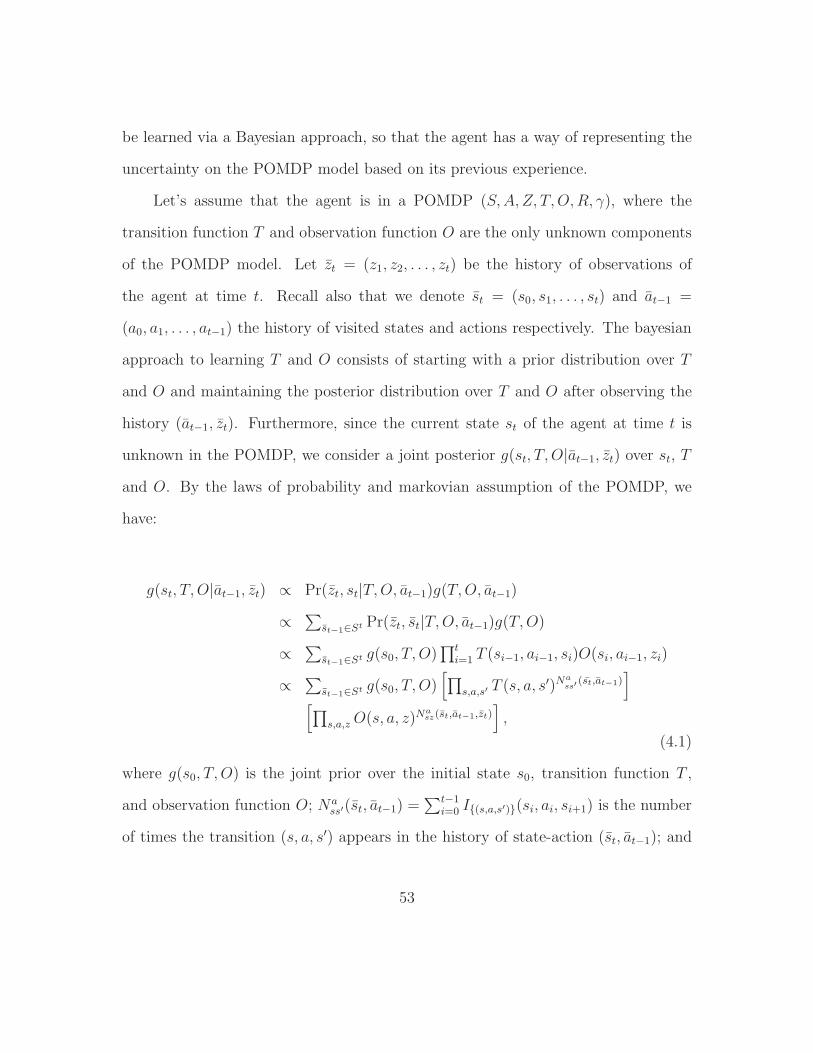
be learned via a Bayesian approach, so that the agent has a way of representing the

uncertainty on the POMDP model based on its previous experience.

Let’s assume that the agent is in a POMDP (S,A, Z, T, O,R, γ), where the

transition function T and observation function O are the only unknown components

of the POMDP model. Let zt = (z1, z2, . . . , zt) be the history of observations of

the agent at time t. Recall also that we denote st = (s0, s1, . . . , st) and at−1 =

(a0, a1, . . . , at−1) the history of visited states and actions respectively. The bayesian

approach to learning T and O consists of starting with a prior distribution over T

and O and maintaining the posterior distribution over T and O after observing the

history (at−1, zt). Furthermore, since the current state st of the agent at time t is

unknown in the POMDP, we consider a joint posterior g(st, T, O|at−1, zt) over st, T

and O. By the laws of probability and markovian assumption of the POMDP, we

have:

g(st, T, O|at−1, zt) ∝ Pr(zt, st|T,O, at−1)g(T,O, at−1)

∝∑

st−1∈St Pr(zt, st|T,O, at−1)g(T,O)

∝∑

st−1∈St g(s0, T, O)∏ti=1 T (si−1, ai−1, si)O(si, ai−1, zi)

∝∑

st−1∈St g(s0, T, O)[

∏

s,a,s′ T (s, a, s′)Nass′

(st,at−1)]

[

∏

s,a,zO(s, a, z)Nasz(st,at−1,zt)

]

,

(4.1)

where g(s0, T, O) is the joint prior over the initial state s0, transition function T ,

and observation function O; Nass′(st, at−1) =

∑t−1i=0 I{(s,a,s′)}(si, ai, si+1) is the number

of times the transition (s, a, s′) appears in the history of state-action (st, at−1); and

53

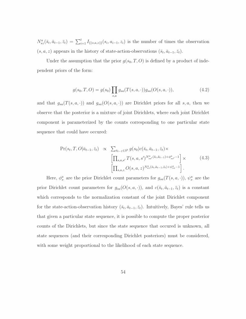
Nasz(st, at−1, zt) =

∑ti=1 I{(s,a,z)}(si, ai−1, zi) is the number of times the observation

(s, a, z) appears in the history of state-action-observations (st, at−1, zt).

Under the assumption that the prior g(s0, T, O) is defined by a product of inde-

pendent priors of the form:

g(s0, T, O) = g(s0)∏

s,a

gsa(T (s, a, ·))gsa(O(s, a, ·)), (4.2)

and that gsa(T (s, a, ·)) and gsa(O(s, a, ·)) are Dirichlet priors for all s, a, then we

observe that the posterior is a mixture of joint Dirichlets, where each joint Dirichlet

component is parameterized by the counts corresponding to one particular state

sequence that could have occured:

Pr(st, T, O|at−1, zt) ∝∑

st−1∈St g(s0)c(st, at−1, zt)×[

∏

s,a,s′ T (s, a, s′)Nass′

(st,at−1)+φass′−1]

×[

∏

s,a,z O(s, a, z)Nasz(st,at−1,zt)+ψasz−1

]

.

(4.3)

Here, φas· are the prior Dirichlet count parameters for gsa(T (s, a, ·)), ψas· are the

prior Dirichlet count parameters for gsa(O(s, a, ·)), and c(st, at−1, zt) is a constant

which corresponds to the normalization constant of the joint Dirichlet component

for the state-action-observation history (st, at−1, zt). Intuitively, Bayes’ rule tells us

that given a particular state sequence, it is possible to compute the proper posterior

counts of the Dirichlets, but since the state sequence that occured is unknown, all

state sequences (and their corresponding Dirichlet posteriors) must be considered,

with some weight proportional to the likelihood of each state sequence.

54

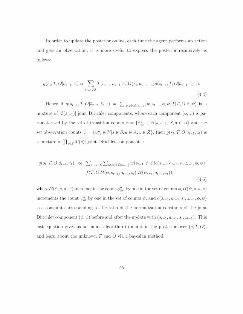
In order to update the posterior online, each time the agent performs an action

and gets an observation, it is more useful to express the posterior recursively as

follows:

g(st, T, O|at−1, zt) ∝∑

st−1∈ST (st−1, at−1, st)O(st, at−1, zt)g(st−1, T, O|at−2, zt−1).

(4.4)

Hence if g(st−1, T, O|at−2, zt−1) =∑

(φ,ψ)∈C(st−1)w(st−1, φ, ψ)f(T,O|φ, ψ) is a

mixture of |C(st−1)| joint Dirichlet components, where each component (φ, ψ) is pa-

rameterized by the set of transition counts φ = {φass′ ∈ N|s, s′ ∈ S, a ∈ A} and the

set observation counts ψ = {ψasz ∈ N|s ∈ S, a ∈ A, z ∈ Z}, then g(st, T, O|at−1, zt) is

a mixture of∏

s∈S |C(s)| joint Dirichlet components :

g(st, T, O|at−1, zt) ∝∑

st−1∈S∑

(φ,ψ)∈C(st−1)w(st−1, φ, ψ)c(st−1, at−1, st, zt−1, φ, ψ)

f(T,O|U(φ, st−1, at−1, st),U(ψ, st, at−1, zt)),

(4.5)

where U(φ, s, a, s′) increments the count φass′ by one in the set of counts φ, U(ψ, s, a, z)

increments the count ψasz by one in the set of counts ψ, and c(st−1, at−1, st, zt−1, φ, ψ)

is a constant corresponding to the ratio of the normalization constants of the joint

Dirichlet component (φ, ψ) before and after the update with (st−1, at−1, st, zt−1). This

last equation gives us an online algorithm to maintain the posterior over (s, T, O),

and learn about the unknown T and O via a bayesian method.

55

4.2 Bayes-Adaptive POMDP

Now that we have a way to maintain the uncertainty over both the state and

model parameters, we would like to address the more interesting question of how to

optimally behave in the environment under such uncertainty, such as to maximize

future expected return. Here we proceed similarly to the Bayes-Adaptive MDP

framework defined in Section 3.2.1.

First notice that the posterior g(st, T, O|at−1, zt) can be seen as a probability

distribution (belief) b over tuples (s, φ, ψ), where each tuple represents a particular

joint Dirichlet component parameterized by the counts (φ, ψ) for a state sequence

ending in state s (i.e. the current state is s), and the probabilities in the belief b

correspond to the mixture weights. Here, we would like to find a policy π for the

agent which maps such beliefs over (s, φ, ψ) to actions a ∈ A. This suggests that the

sequential decision problem of optimally behaving under state and model uncertainty

can be modeled as a POMDP over hyperstates of the form (s, φ, ψ). This is exactly

how we proceed to define the BAPOMDP.

Consider the new POMDP (S ′, A′, Z ′, P ′, R′). As was just mentionned, the new

states (hyperstates) are tuples of the form (s, φ, ψ) and the actions performed by the

agent should be actions that the agent can do in the original POMDP. Hence the

set of hyperstates is defined as S ′ = S × T × O, where T = {φ ∈ N|S|2|A||∀(s, a) ∈

S × A,∑

s′∈S φass′ > 0} and O = {ψ ∈ N

|S||A||Z||∀(s, a) ∈ S × A,∑

z∈Z ψasz > 0}, and

the new set of actions A′ = A. As in the definition of the Bayes-adaptive MDP, the

constraints on the count parameters φ and ψ are only to ensure that the transition-

observation probabilities, as defined below, are well defined. The observations that

56

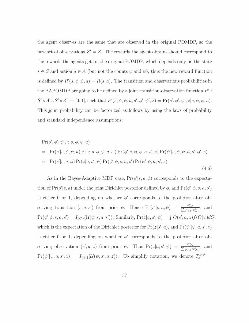
the agent observes are the same that are observed in the original POMDP, so the

new set of observations Z ′ = Z. The rewards the agent obtains should correspond to

the rewards the agents gets in the original POMDP, which depends only on the state

s ∈ S and action a ∈ A (but not the counts φ and ψ), thus the new reward function

is defined by R′(s, φ, ψ, a) = R(s, a). The transition and observations probabilities in

the BAPOMDP are going to be defined by a joint transition-observation function P ′ :

S ′×A′×S ′×Z ′ → [0, 1], such that P ′(s, φ, ψ, a, s′, φ′, ψ′, z) = Pr(s′, φ′, ψ′, z|s, φ, ψ, a).

This joint probability can be factorized as follows by using the laws of probability

and standard independence assumptions:

Pr(s′, φ′, ψ′, z|s, φ, ψ, a)

= Pr(s′|s, φ, ψ, a) Pr(z|s, φ, ψ, a, s′) Pr(φ′|s, φ, ψ, a, s′, z) Pr(ψ′|s, φ, ψ, a, s′, φ′, z)

= Pr(s′|s, a, φ) Pr(z|a, s′, ψ) Pr(φ′|φ, s, a, s′) Pr(ψ′|ψ, a, s′, z).

(4.6)

As in the Bayes-Adaptive MDP case, Pr(s′|s, a, φ) corresponds to the expecta-

tion of Pr(s′|s, a) under the joint Dirichlet posterior defined by φ, and Pr(φ′|φ, s, a, s′)

is either 0 or 1, depending on whether φ′ corresponds to the posterior after ob-

serving transition (s, a, s′) from prior φ. Hence Pr(s′|s, a, φ) =φass′

∑

s′′∈S φass′′

, and

Pr(φ′|φ, s, a, s′) = I{φ′}(U(φ, s, a, s′)). Similarly, Pr(z|a, s′, ψ) =∫

O(s′, a, z)f(O|ψ)dO,

which is the expectation of the Dirichlet posterior for Pr(z|s′, a), and Pr(ψ′|ψ, a, s′, z)

is either 0 or 1, depending on whether ψ′ corresponds to the posterior after ob-

serving observation (s′, a, z) from prior ψ. Thus Pr(z|a, s′, ψ) =ψas′z

∑

z′∈Z ψas′z′

, and

Pr(ψ′|ψ, a, s′, z) = I{ψ′}(U(ψ, s′, a, z)). To simplify notation, we denote T sas′

φ =

57

φass′

∑

s′′∈S φass′′

and Os′azψ =

ψas′z

∑

z′∈Z ψas′z′

. It follows that the joint transition-observation

probabilities in the BAPOMDP are defined by:

Pr(s′, φ′, ψ′, z|s, φ, ψ, a)

= T sas′

φ Os′azψ I{φ′}(U(φ, s, a, s′))I{ψ′}(U(ψ, s′, a, z)).

(4.7)

Hence, the BAPOMDP defined by the POMDP (S ′, A′, Z ′, P ′, R′) has a known

model and characterizes the problem of optimal sequential decision-making in POMDP

(S,A, Z, T, O,R) with uncertainty on the transition T and observation functions O

described by Dirichlet distributions.

An alternative interpretation of the BAPOMDP is as follows: given the un-

known state sequence that occured since the beggining, one can compute exactly the

posterior counts φ and ψ. Thus there exists a unique (φ,ψ) reflecting the correct

posterior counts according to the state sequence that occured, but these correct pos-

terior counts are only partially observable through the observations z ∈ Z obtained

by the agent, similarly to the current hidden state s ∈ S of the agent. Thus (φ, ψ) can

simply be thought as other hidden state variables that the agent tracks via the belief

state, based on its observations. The BAPOMDP formulates the decision problem

of optimal sequential decision-making under partial observability of both the state

s ∈ S, and posterior counts (φ, ψ).

The belief state in the BAPOMDP corresponds exactly to the posterior defined

in the previous section (Equation 4.3). By maintaining this belief, the agent main-

tains its uncertainty on the POMDP model and learns about the unknown transition

and observations functions. Initially, if φ0 and ψ0 represent the prior Dirichlet count

58

parameters (i.e. the agent’s prior knowledge of T and O), and b0 the initial state

distribution of the unknown POMDP, then the initial belief b′0 of the BAPOMDP is

defined as b′0(s, φ, ψ) = b0(s)I{φ0}(φ)I{ψ0}(ψ). Since the BAPOMDP is just a POMDP

with an infinite number of states, the belief update and value function equations pre-

sented in Section 2.2.1 can be applied directly to the BAPOMDP model. However,

since there are infinitely many hyperstates, these calculations can be performed ex-

actly in practice only if the number of probable hyperstates in the belief is finite.

The following theorem shows that this is the case at any finite time t:

Theorem 4.2.1. Let (S ′, A, Z, P ′, R′, γ) be a BAPOMDP constructed from the POMDP

(S,A, Z, T, O,R, γ). If S is finite, then at any time t, the set S ′b′t

= {σ ∈ S ′|b′t(σ) > 0}

has size |S ′b′t| ≤ |S|t+1.

Proof. Proof available in Appendix A.

The proof of this theorem suggests that it is sufficient to iterate over S and S ′b′t−1

in order to compute the belief state b′t when an action and observation are taken in

the environment. Hence, Algorithm 1 can be used to update the belief state online.

Algorithm 1 Exact Belief Update in BAPOMDP.function τ(b, a, z)Initialize b′ as a 0 vector.for all (s, φ, ψ) ∈ S′

b do

for all s′ ∈ S do

φ′ ← U(φ, s, a, s′)ψ′ ← U(ψ, s′, a, z)b′(s′, φ′, ψ′)← b′(s′, φ′, ψ′) + b(s, φ, ψ)T sas

′

φ Os′azψ

end for

end for

return normalized b′

59

The value function of a BAPOMDP for finite horizons can be represented by a

finite set Γ of functions α : S ′ → R, as in standard POMDP. This is shown formally

in the following theorem:

Theorem 4.2.2. For any horizon t, there exists a finite set Γt of functions S ′ → R,

such that V ∗t (b) = maxα∈Γt

∑

σ∈S′ α(σ)b(σ).

Proof. Proof available in Appendix A.

The proof of this theorem shows that as in a POMDP, an exact solution of

the BAPOMDP can be computed using dynamic programming, by incrementally

constructing the set of α-functions that defines the value function as follows (see [44]

for more details):

Γa1 = {αa|αa(s, φ, ψ) = R(s, a)},

Γa,zt = {αa,zi |αa,zi (s, φ, ψ) = γ

∑

s′∈S Tsas′

φ Os′azψ α′

i(s′,U(φ, s, a, s′),U(ψ, s′, a, z)),

α′i ∈ Γt−1},

Γat = Γa1 ⊕ Γa,z1t ⊕ Γa,z2t ⊕ · · · ⊕ Γa,z|Z|

t , (where ⊕ is the cross sum operator),

Γt =⋃

a∈A Γat .

(4.8)

However, in practice, it will be impossible to compute αa,zi (s, φ, ψ) for all (s, φ, ψ) ∈

S ′, unless a particular finite parametric form for the α-functions is used. Hence, the

next section shows that the infinite state space can be reduced to a finite state space,

while still preserving the value function to arbitrary precision for any horizon t. This

yields an approximate finite representation of the α-functions, that can achieve any

desired precision.

60

4.3 Finite Model Approximation

Solving the BAPOMDP exactly for all belief states is impossible in practice due

to the dimensionnality of the state space (in particular to the fact that the count

vectors can grow unbounded). The first proposed method to address this problem

is to reduce this infinite state space to a finite state space, while preserving the

value function of the BAPOMDP to arbitrary precision. This allows us to compute

an ε-optimal value function over the resulting finite-dimensionnal belief space using

standard POMDP techniques.

The main intuition behind the compression of the state space presented here

is that, as the Dirichlet counts grow larger and larger, the transition and observa-

tion probabilities defined by these counts do not change much when the counts are

incremented by one. Hence, there should exist a point where if we simply stop in-

crementing the counts, the value function of that approximate BAPOMDP (where

the counts are bounded) approximates the value function of the BAPOMDP within

some ε > 0. If we can bound above the counts in such a way, this ensures that the

state space will be finite.

In order to find such a bound on the counts, we begin by deriving an upper bound

on the value difference between two hyperstates that differ only by their model es-

timates φ and ψ. This bound uses the following definitions: given φ, φ′ ∈ T , and

ψ, ψ′ ∈ O, defineDsaS (φ, φ′) =

∑

s′∈S∣

∣T sas′

φ − T sas′

φ′

∣

∣,DsaZ (ψ, ψ′) =

∑

z∈Z∣

∣Osazψ −O

sazψ′

∣

∣,

N saφ =

∑

s′∈S φass′, and N sa

ψ =∑

z∈Z ψasz.

61

Theorem 4.3.1. Given any φ, φ′ ∈ T , ψ, ψ′ ∈ O, and γ ∈ (0, 1), then for all t:

supαt∈Γt,s∈S

|αt(s, φ, ψ)− αt(s, φ′, ψ′)| ≤ 2γ||R||∞(1−γ)2 sup

s,s′∈S,a∈A

[

DsaS (φ, φ′) +Ds′a

Z (ψ, ψ′)

+ 4ln(γ−e)

(

∑

s′′∈S|φass′′−φ′ass′′ |

(N saφ +1)(N sa

φ′+1)

+∑

z∈Z|ψas′z−ψ′as′z|

(N s′aψ +1)(N s′a

ψ′ +1)

)]

.

Proof. Proof available in Appendix A.

We now use this bound on the α-vector values to approximate the space of

Dirichlet parameters within a finite subspace. We use the following definitions: given

any ε > 0, define ε′ = ε(1−γ)28γ||R||∞ , ε′′ = ε(1−γ)2 ln(γ−e)

32γ||R||∞ , N εS = max

(

|S|(1+ε′)ε′

, 1ε′′− 1

)

and

N εZ = max

(

|Z|(1+ε′)ε′

, 1ε′′− 1

)

.

Theorem 4.3.2. Given any ε > 0 and (s, φ, ψ) ∈ S ′ such that ∃a ∈ A, s′ ∈ S,

N s′aφ > N ε

S or N s′aψ > N ε

Z , then ∃(s, φ′, ψ′) ∈ S ′ such that ∀a ∈ A, s′ ∈ S, N s′aφ′ ≤ N ε

S

and N s′aψ′ ≤ N ε

Z where |αt(s, φ, ψ)− αt(s, φ′, ψ′)| < ε holds for all t and αt ∈ Γt.

Proof. Proof available in Appendix A.

Theorem 4.3.2 suggests that if we want a precision of ε on the value function,

we just need to restrict the space of Dirichlet parameters to count vectors φ ∈ Tε =

{φ ∈ N|S|2|A||∀a ∈ A, s ∈ S, 0 < N sa

φ ≤ N εS} and ψ ∈ Oε = {ψ ∈ N

|S||A||Z||∀a ∈ A, s ∈

S, 0 < N saψ ≤ N ε

Z}. While an argument based on the discount factor could easily

be made to bound the counts based on a particular prior (in which case the bound

would depend on the prior counts plus some constant), the previous bound do not

depend on the prior at all. This is convenient as it will allow us to solve one finite

POMDP and use its solution to define a (near-)optimal policy for any prior we may

want to choose afterwards.

62

Since Tε and Oε are finite, we can define a finite approximate BAPOMDP as

the tuple (Sε, A, Z, Tε, Oε, Rε, γ) where Sε = S × Tε × Oε is the finite state space.

To define the transition and observation functions over that finite state space, we

need to make sure that when the count vectors are incremented, they stay within

the finite space. To achieve, this we define a projection operator Pε : S ′ → Sε that

simply projects every state in S ′ to their closest state in Sε.

Definition 4.3.1. Let d : S ′ × S ′ → R be defined such that:

d(s, φ, ψ, s′, φ′, ψ′) =

2γ||R||∞(1−γ)2 sup

s,s′∈S,a∈A

[

DsaS (φ, φ′) +Ds′a

Z (ψ, ψ′)

+ 4ln(γ−e)

(

∑

s′′∈S |φass′′

−φ′ass′′

|(N as

φ +1)(N asφ′

+1)+

∑

z∈Z |ψas′z

−ψ′as′z

|(N as′

ψ +1)(N as′

ψ′ +1)

)]

,if s = s′

8γ||R||∞(1−γ)2

(

1 + 4ln(γ−e)

)

+ 2||R||∞(1−γ) , otherwise.

Definition 4.3.2. Let Pε : S ′ → Sε be defined as Pε(s) = argmins′∈Sε

d(s, s′)

The function d uses the bound defined in Theorem 4.3.1 as a distance between

states that only differ in their φ and ψ vectors, and uses an upper bound on that

value when the states differ. Thus Pε always maps states (s, φ, ψ) ∈ S ′ to some

state (s, φ′, ψ′) ∈ Sε. Note that if σ ∈ Sε, then Pε(σ) = σ. Using Pε, the joint

transition-observation function is defined as follows:

Pε(s, φ, ψ, a, s′, φ′, ψ′, z) = T sas

′

φ Os′azψ I{(s′,φ′,ψ′)}(Pε(s

′,U(φ, s, a, s′),U(ψ, s′, a, z))).

(4.9)

This definition is the same as the one in the BAPOMDP, except that now an

extra projection is added to make sure that the incremented count vectors stay in Sε.

Finally, the reward function Rε : Sε ×A→ R is defined as Rε((s, φ, ψ), a) = R(s, a).

The finite POMDP (Sε, A, Z, Pε, Rε) can thus be used to approximate the original

BAPOMDP model.

63

Theorem 4.3.3 bounds the value difference between α-vectors computed with

this finite model and the α-vectors computed with the original model.

Theorem 4.3.3. Given any ε > 0, (s, φ, ψ) ∈ S ′ and αt ∈ Γt computed from

the BAPOMDP. Let αt be the α-vector representing the same contingency plan as

αt but computed with the finite POMDP (Sε, A, Z, Pε, Rε, γ), then |αt(Pε(s, φ, ψ))−

αt(s, φ, ψ)| < ε1−γ .

Proof. Proof available in Appendix A.

Because the state space is now finite, offline solution methods from the literature

on finite POMDPs could potentially be applied. However, even though the state

space is finite, it will generally be very large for small ε, such that it may still

be intractable, even for small domains. Hence in the next two sections, a more

tractable alternative approach is presented. This approach solves the BAPOMDP

online, by trying only to find the best immediate action to perform in the current

belief of the agent, as in online POMDP solution methods (Section 2.2.2). The

advantage here is that no finite approximation of the state space is required in this

approach. However, because maintaining the exact belief in the BAPOMDP becomes

intractable (exponential in the history lenght, as shown in Theorem 4.2.1), several

polynomial-time approximations of the belief update computations are proposed.

These polynomial-time approximations of the belief are leveraged in the proposed

online planning algorithm, in order to efficiently compute beliefs that may be reached

in the future from the current belief of the agent. The different approximate belief

monitoring algorithms are presented in the next section and then the online planning

algorithm is introduced afterwards.

64

4.4 Approximate Belief Monitoring

As shown in Theorem 4.2.1, the number of states with non-zero probability

grows exponentially in the current time, thus exact belief monitoring can quickly

become intractable. We now discuss different particle filter approximations that

allow polynomial-time belief tracking.

Monte Carlo sampling: Monte Carlo sampling algorithms have been widely

used for sequential state estimation [17]. Given a prior belief b, followed by ac-

tion a and observation z, the new belief b′ is obtained by first sampling K states

from the distribution b, then for each sampled s a new state s′ is sampled from

T (s, a, ·). Finally, the probability O(s′, a, z) is added to b′(s′) and the belief b′ is

re-normalized. This will capture at most K states with non-zero probabilities. In

the context of BAPOMDPs, we use a slight variation of this method, where (s, φ, ψ)

are first sampled from b, and then a next state s′ ∈ S is sampled from the conditional

distribution Pr(s′|s, φ, ψ, a, z) ∝ T sas′

φ Os′azψ . The probability 1/K is added directly

to b′(s′,U(φ, s, a, s′),U(ψ, s′, a, z)).

Most Probable: Another possibility is to perform the exact belief update at

a given time step, but then only keep the K most probable states in the new belief

b′ and renormalize b′. This minimizes the L1 distance between the exact belief b′

and the approximate belief maintained with K particles1 . While keeping only the

K most probable particles biases the belief of the agent, this can still be a good

1 The L1 distance between two beliefs b and b′, denoted ||b − b′||1, is defined as∑

σ∈S′ |b(σ − b′(σ)|

65

approach in practice as minimizing the L1 distance bounds the difference between

the values of the exact and approximate belief: i.e. |V ∗(b)−V ∗(b′)| ≤ ||R||∞1−γ ||b− b

′||1.

Weighted Distance Minimization: A potentially better way to minimize

the difference in value function between the approximate and exact belief state is to

use the tighter upper bound on the value difference defined in the previous section.

Hence, in order to keep the K particles which best approximate the exact belief’s

value, an exact belief update is performed and then the K particles which minimize a

weighted sum of distance measures, where distance is defined as in Definition 4.3.1,

are kept to approximate the exact belief. A greedy approximate algorithm that

achieves this is described in Algorithm 2. Again, this procedure biases the belief,

but may yield better performance in practice.

Algorithm 2 Weighted Distance Belief Update in BAPOMDP.function WD(b, a, z,K)b′ ← τ(b, a, z)Initialize b′′ as a 0 vector.(s, φ, ψ)← argmax(s′,φ′,ψ′)∈S′

b′b′(s′, φ′, ψ′).

b′′(s, φ, ψ)← b′(s, φ, ψ)for i = 2 to K do

(s, φ, ψ)← argmax(s′,φ′,ψ′)∈S′b′b′(s′, φ′, ψ′)min(s′′,φ′′,ψ′′)∈S′

b′′d(s′, φ′, ψ′, s′′, φ′′, ψ′′)

b′′(s, φ, ψ)← b′(s, φ, ψ)end for

return normalized b′′

4.5 Online Planning

While the finite model presented in Section 4.3 can be used to find provably near-

optimal policies offline, this will likely be intractable in practice due to the very large

state space required to ensure good precision. Instead, we turn to online lookahead

search algorithms, which have been proposed for solving standard POMDPs [55].

66

Our approach simply performs dynamic programming over all the beliefs reachable

within some fixed finite planning horizon from the current belief. The action with

highest return over that finite horizon is executed and then planning is conducted

again on the next belief. To further limit the complexity of the online planning

algorithm, the approximate belief monitoring methods detailed above are used to

compute reachable beliefs. The overall complexity is in O((|A||Z|)DCb) where D is

the planning horizon and Cb is the complexity of updating the belief. Algorithm 3

describes the planning algorithm in detail.

Algorithm 3 Online Planning Algorithm for BAPOMDP.

function V (b, d, k)if d = 0 then

return 0end if

maxQ← −∞for all a ∈ A do

q ← R(b, a)for all z ∈ Z do

b′ ← ParticleFilter(b, a, z, k)q ← q + γ Pr(z|b, a)V (b′, d− 1, k)

end for

if q > maxQ then

maxQ← q

maxA← a

end if

end for

if d = D then

a← maxA

end if

return maxQ

At each step, the agent computes V (b,D,K) for its current belief b and then

executes the action a stored by the algorithm. In the previous algorithm, R(b, a)

67

corresponds to the expected immediate reward obtained by doing action a in be-

lief b, i.e. R(b, a) =∑

(s,φ,ψ)∈S′bb(s, φ, ψ)R(s, a), and Pr(z|b, a) corresponds to the

probability of observing z after doing action a in belief b:

Pr(z|b, a) =∑

s′∈S

∑

(s,φ,ψ)∈S′b

T sas′

φ Os′azψ b(s, φ, ψ). (4.10)

ParticleFilter(b, a, z, k) calls the chosen approximate belief monitoring algorithm

(e.g. Algorithm 2) and returns an updated belief with k particles.

4.6 Experimental Results

We begin by evaluating the different belief approximations introduced above.

To do so, we use a simple online D-step lookahead search, and compare the over-

all expected return and model accuracy in two different problems: the well-known

Tiger [44] and a domain called Follow [63]. Given T (s, a, s′) and O(s′, a, z) the exact

probabilities of the (unknown) POMDP, the model accuracy is measured in terms of

the weighted sum of L1 distance, denoted WL1, between the exact model and the

probable models in a belief state b:

WL1(b) =∑

(s,φ,ψ)∈S′bb(s, φ, ψ)L1(φ, ψ)

L1(φ, ψ) =∑

a∈A∑

s′∈S[∑

s∈S |Tsas′

φ − T (s, a, s′)|+∑

z∈Z |Os′azψ −O(s′, a, z)|

]

(4.11)

4.6.1 Tiger

In the Tiger problem [44], we consider the case where the transition and re-

ward parameters are known, but the observation probabilities are not. Hence,

there are four unknown parameters: OLl, OLr, ORl, ORr (OLr stands for Pr(z =

hear right|s = tiger Left, a = Listen)). We define the observation count vector

68

ψ = [ψLl, ψLr, ψRl, ψRr]. We consider a prior of ψ0 = [5, 3, 3, 5], which specifies an

expected sensor accuracy of 62.5% (instead of the correct 85%) in both states. Each

simulation consists of 100 episodes. Episodes terminate when the agent opens a door,

at which point the POMDP state (i.e. tiger’s position) is reset, but the distribution

over count vectors is carried over to the next episode.

Figures 4–1 and 4–2 show how the average return and model accuracy evolve

over the 100 episodes (results are averaged over 1000 simulations), using an online 3-

step lookahead search with varying belief approximations and parameters. Returns

obtained by planning directly with the prior and exact model (without learning)

are shown for comparison. Model accuracy is measured on the initial belief of each

episode. Figure 4–3 compares the average planning time per action taken by each

approach. We observe from these figures that the results for the Most Probable

and Weighted Distance belief update approximations are very similar and perform

well even with few particles (lines are overlapping in many places, making Weighted

Distance results hard to see). On the other hand, the performance of the Monte

Carlo approximation is significantly affected by the number of particles and requires

many more particles (64) to obtain an improvement over the prior. This may be due

to the sampling error that is introduced when using fewer samples.

4.6.2 Follow

Next we consider the POMDP domain, called Follow, inspired by an interactive

human-robot task [63]. It is often the case that such domains are particularly suscep-

tible to parameter uncertainty (due to the difficulty in modelling human behavior),

thus this environment motivates the utility of Bayes-Adaptive POMDPs in a very

69

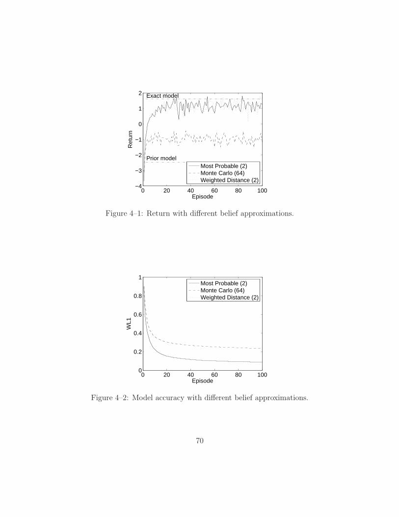
0 20 40 60 80 100−4

−3

−2

−1

0

1

2

Episode

Ret

urn

Most Probable (2)Monte Carlo (64)Weighted Distance (2)

Prior model

Exact model

Figure 4–1: Return with different belief approximations.

0 20 40 60 80 1000

0.2

0.4

0.6

0.8

1

Episode

WL1

Most Probable (2)Monte Carlo (64)Weighted Distance (2)

Figure 4–2: Model accuracy with different belief approximations.

70

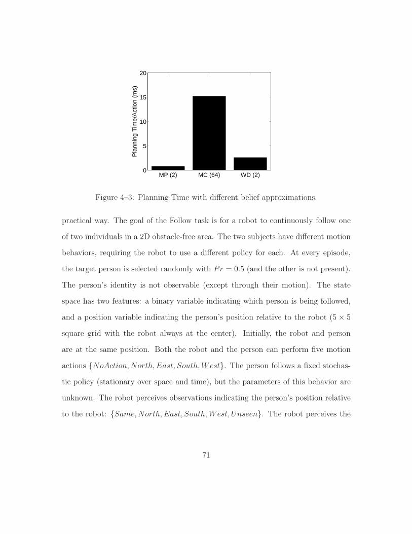
MP (2) MC (64) WD (2)0

5

10

15

20

Pla

nnin

g T

ime/

Act

ion

(ms)

Figure 4–3: Planning Time with different belief approximations.

practical way. The goal of the Follow task is for a robot to continuously follow one

of two individuals in a 2D obstacle-free area. The two subjects have different motion

behaviors, requiring the robot to use a different policy for each. At every episode,

the target person is selected randomly with Pr = 0.5 (and the other is not present).

The person’s identity is not observable (except through their motion). The state

space has two features: a binary variable indicating which person is being followed,

and a position variable indicating the person’s position relative to the robot (5 × 5

square grid with the robot always at the center). Initially, the robot and person

are at the same position. Both the robot and the person can perform five motion

actions {NoAction,North, East, South,West}. The person follows a fixed stochas-

tic policy (stationary over space and time), but the parameters of this behavior are

unknown. The robot perceives observations indicating the person’s position relative

to the robot: {Same,North, East, South,West, Unseen}. The robot perceives the

71

correct observation with probability 0.8 and Unseen with probability 0.2. The re-

ward R = +1 if the robot and person are at the same position (central grid cell),

R = 0 if the person is one cell away from the robot, and R = −1 if the person is two

cells away. The task terminates if the person reaches a distance of 3 cells away from

the robot (i.e. the person exits the 5× 5 square grid), also causing a reward of -20.

We use a discount factor of 0.9.

When formulating the BAPOMDP, the robot’s motion model (deterministic),

the observation probabilities and the rewards are assumed to be known. We maintain

a separate count vector for each person, representing the number of times they move

in each direction, i.e. φ1 = [φ1NA, φ

1N , φ

1E, φ

1S, φ

1W ], φ2 = [φ2

NA, φ2N , φ

2E, φ

2S, φ

2W ]. We

assume a prior φ10 = [2, 3, 1, 2, 2] for person 1 and φ2

0 = [2, 1, 3, 2, 2] for person 2, while

in reality person 1 moves with probabilities [0.3, 0.4, 0.2, 0.05, 0.05] and person 2 with

probabilities [0.1, 0.05, 0.8, 0.03, 0.02]. We run 200 simulations, each consisting of 100

episodes (of at most 10 time steps). The count vectors’ distributions are reset (to the

prior) after every simulation, and the target person is (randomly) reset after every

episode. We use a 2-step lookahead search for planning in the BAPOMDP.

Figures 4–4 and 4–5 show how the average return and model accuracy evolve

over the 100 episodes (averaged over the 200 simulations) with different belief ap-

proximations. Figure 4–6 compares the planning time taken by each approach. We

observe from these figures that the results for the Weighted Distance approximations

are much better both in terms of return and model accuracy, even with fewer par-

ticles (16). Monte Carlo fails at providing any improvement over the prior model,

which suggests it would require many more particles. Running Weighted Distance

72

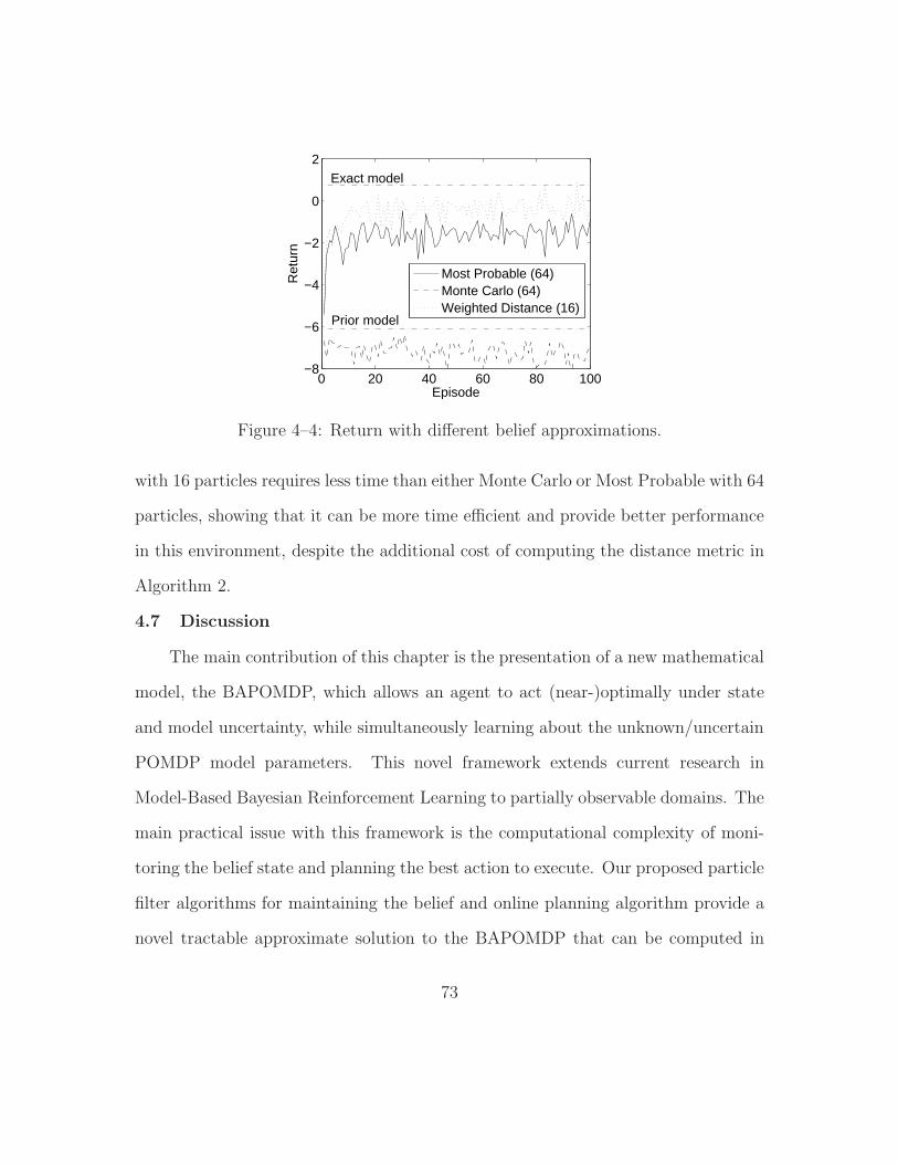
0 20 40 60 80 100−8

−6

−4

−2

0

2

Episode

Ret

urn

Most Probable (64)Monte Carlo (64)Weighted Distance (16)

Prior model

Exact model

Figure 4–4: Return with different belief approximations.

with 16 particles requires less time than either Monte Carlo or Most Probable with 64

particles, showing that it can be more time efficient and provide better performance

in this environment, despite the additional cost of computing the distance metric in

Algorithm 2.

4.7 Discussion

The main contribution of this chapter is the presentation of a new mathematical

model, the BAPOMDP, which allows an agent to act (near-)optimally under state

and model uncertainty, while simultaneously learning about the unknown/uncertain

POMDP model parameters. This novel framework extends current research in

Model-Based Bayesian Reinforcement Learning to partially observable domains. The

main practical issue with this framework is the computational complexity of moni-

toring the belief state and planning the best action to execute. Our proposed particle

filter algorithms for maintaining the belief and online planning algorithm provide a

novel tractable approximate solution to the BAPOMDP that can be computed in

73

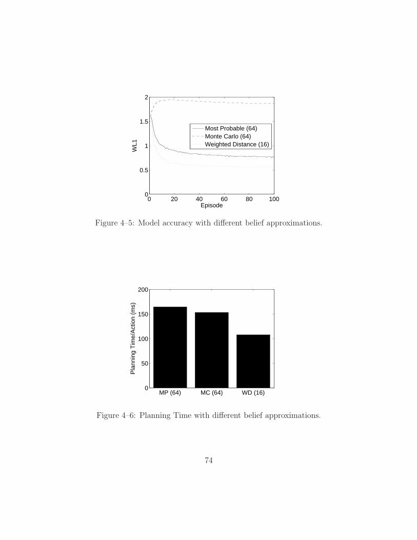
0 20 40 60 80 1000

0.5

1

1.5

2

Episode

WL1

Most Probable (64)Monte Carlo (64)Weighted Distance (16)

Figure 4–5: Model accuracy with different belief approximations.

MP (64) MC (64) WD (16)0

50

100

150

200

Pla

nnin

g T

ime/

Act

ion

(ms)

Figure 4–6: Planning Time with different belief approximations.

74

polynomial-time. This algorithmic solution allows to trade-off between solution qual-

ity and computation time by changing the number of particles K and the planning

horizon D. Finally, another theoretical contribution is the presentation of a finite

POMDP approximation of the BAPOMDP model, which could also be adapted to

the Bayes-Adaptive MDP, in order to approximate it by a finite MDP.

However, the online planning algorithm is relatively inefficient as it must explore

all future sequences of D actions and observations. It would be possible to make it

more efficient by adopting heuristic search methods similar to other online planning

algorithms for POMDPs (Section 2.2.2). However, these methods rely on informative

lower and upper bound computed offline, and we haven’t yet found an efficient way

of computing such bounds on the BAPOMDP’s value function. Thus, this could be

an important area for future research.

Another avenue for future research is to generalize the current framework to

the case where the number of states is unknown. Since the states are not observed,

knowning the number of states is a strong assumption in practice. In the case

where the number of states is unknown, we believe that Dirichlet Process priors and

posteriors could be used to learn the transition and observation dynamics [2].

Finally, it would also be useful to analyse the convergence of the posterior dis-

tribution over models. One issue in partially observable domains is that there may

be several different models (in terms of state dynamics) which produce the same

action/observation sequences with the same probabilities. This implies that if these

models all have equal likelihood in the prior, then the posterior may converge to-

wards a multimodal distribution, with a mode for each undistinguishable model.

75

While this doesn’t pose any problems for predicting future observation sequences,

it causes some problems in terms of predicting future rewards, as these depend on

the state dynamics, which may vary between these undistinguishable models. We

believe such problems can be overcome if the rewards are part of the observations

and the reward model is learned at the same time, however more analysis may be

needed here.

76

CHAPTER 5

Bayesian Reinforcement Learning in Continuous Domains

The previously presented frameworks for model-based BRL, the BAMDP and

BAPOMDP, are only applicable in domains described by finite sets of states, actions

and observations, as the Dirichlet can only be used as a posterior over discrete distri-

butions. This is an important limitation in practice as many practical problems are

naturally described by continuous states, continuous actions and continuous observa-

tions. For instance, in robot navigation problems, the state is normally described by

continuous variables such as the robot’s position, orientation, velocity and angular

velocity; the choice of action controls the forward and angular acceleration, which are

both continuous; and the observations provide a noisy estimate of the robot’s state

based on its sensors, which would also be continuous. Our goal in this chapter is to

present an extension of the model-based BRL framework that can handle domains

that are both partially observable and continuous. To achieve this, we propose an

adaptation of the BAPOMDP framework presented in Chapter 4 to handle domains

described by continuous states, continuous actions and continuous observations. The

proposed approach involves using a bayesian technique to learn the unknown param-

eters of a particular continuous parametric distribution specifying the transition and

observation dynamics of the system. For simplicity of presentation, we focus here on

the case where these parametric distributions are multivariate Gaussian distributions

with unknown mean vector and covariance matrix. However, the framework can be

77

easily extended to other families of distributions or more complex models, such as a

mixture of Gaussian model.

In this chapter, we first present the parameterized form of the continuous POMDP

model used in this chapter, and describe how to learn this parameterized form with

a bayesian learning approach. From this approach, the Bayes-Adaptive Continuous

POMDP model (BACPOMDP) is then introduced. However, its optimal solution

and belief update equations are shown to be integrals with no known closed-form so-

lutions. A Monte Carlo integration approach is proposed to approximately maintain

the belief and find an approximate solution. This Monte Carlo approach is essentially

an adaptation of the Monte Carlo particle filter and online planning algorithm for

solving the BAPOMDP model (Sections 4.4 and 4.5), to the BACPOMDP model.

5.1 Continuous POMDP

In a continuous POMDP, the set of states S ⊆ Rm, set of actions A ⊆ R

n and

set of observations Z ⊆ Rp are all continuous and possibly multidimensional. It

is assumed here that m, n and p are finite and A is closed and bounded1 . The

transition function T specifies the probability density function (p.d.f.) T (s, a, s′) =

f(s′|s, a) ∈ [0,∞] over the next state s′ ∈ S for any current state s and action a

executed by the agent, such that∫

ST (s, a, s′)ds′ = 1 for all s ∈ S, a ∈ A. Similarly,

the observation function O specifies the p.d.f. O(s′, a, z) = f(z|s′, a) ∈ [0,∞] over

the observations z ∈ Z obtained by the agent for any state s′ and previous action a.

1 The constraints on A are to ensure existence of an optimal solution within A. Itis not necessary for S and Z to be closed or bounded.

78

It is assumed in this chapter that the functions T and O are defined through a

Gaussian model of the following form:

st = GT (st−1, at−1, Xt) Xt ∼ Nk(µX ,ΣX),

zt = GO(st, at−1, Yt) Yt ∼ Nl(µY ,ΣY ),(5.1)

where st, at and zt represent the state, action and observation at time t, Xt ∈ Rk and

Yt ∈ Rl are Gaussian noise vector random variables, GT is a function that returns

the next state (given the previous state, previous action and gaussian noise), and GO

is a function that returns the observation (given the current state, previous action

and gaussian noise). It is assumed in this chapter that GT |s,a(x) = GT (s, a, x) is a

1-1 mapping from Rk to S, for all s ∈ S, a ∈ A, such that the inverse G−1

T |s,a(s′)

exists; and that GO|s,a(y) = GO(s, a, y) is a 1-1 mapping from Rl to Z, for all s ∈ S,

a ∈ A, such that G−1O|s,a(z) exists. These two assumptions are satisfied by any linear

Gaussian model, including the basic additive Gaussian noise model, as well as some

nonlinear Gaussian models.

In a continuous POMDP, the belief state is a p.d.f. over S and can be updated

via Bayes’ rule, using an equation similar to Equation 2.13:

bt(s′) =

1

f(zt|bt−1, at−1)O(s′, at−1, zt)

∫

S

T (s, at−1, s′)bt−1(s)ds, (5.2)

where:

f(zt|bt−1, at−1) =

∫

S

O(s′, at−1, zt)

∫

S

T (s, at−1, s′)bt−1(s)dsds

′, (5.3)

is the probability density of observing zt after doing action at−1 in belief bt−1.

79

Similarly the optimal value function is obtained via an equation similar to Equa-

tion 2.16:

V ∗(b) = maxa∈A

[∫

S

b(s)R(s, a)ds+

∫

Z

f(z|b, a)V ∗(τ(b, a, z))dz

]

. (5.4)

5.2 Bayesian Learning of a Continuous POMDP

In order to introduce the Bayes-Adaptive Continuous POMDP framework for

model-based BRL in a continuous POMDP of the form presented in the previous

section, we first show how the model of a standard continuous POMDP can be

learned via a bayesian approach.

Let’s assume that the agent is in a continuous POMDP as defined in the pre-

vious section, where the mean vectors (µX , µY ) and covariance matrices (ΣX , ΣY )

of the Gaussian noise random variables X and Y are the only unknown parame-

ters of the continuous POMDP (i.e. GT and GO are assumed to be known func-

tions). Recall that we denote st = (s0, s1, . . . , st), at−1 = (a0, a1, . . . , at−1) and

zt = (z1, z2, . . . , zt) the history of visited states, actions and observations respec-

tively. Our goal is to learn (µX ,ΣX) and (µY ,ΣY ) using a bayesian approach from

the history of actions and observations (at−1, zt). First notice that the posterior dis-

tribution g(st, µX ,ΣX , µY ,ΣY |at−1, zt) over the hidden state st and unknown mean

and covariance parameters (µX ,ΣX , µY ,ΣY ) can be expressed as follows:

g(st, µX ,ΣX , µY ,ΣY |at−1, zt) =∫

Stf(st, µX ,ΣX , µY ,ΣY |at−1, zt)dst−1

=∫

Stg(µX,ΣX , µY ,ΣY |st, at−1, zt)f(st|at−1, zt)dst−1

(5.5)

80

The term f(st|at−1, zt) is proportional to the likelihood of state-observation sequence

(st, zt) under the prior g(µX ,ΣX , µY ,ΣY ) for the given action sequence at−1:

f(st|at−1, zt) ∝

∫

f(st, zt|µX ,ΣX , µY ,ΣY , at−1)g(µX,ΣX , µY ,ΣY )d(µX ,ΣX , µY ,ΣY ),

(5.6)

while the previous term, g(µX,ΣX , µY ,ΣY |st, at−1, zt), corresponds to the poste-

rior over (µX ,ΣX , µY ,ΣY ) given a known state-action-observation sequence defined

by (st, at−1, zt). This posterior can be defined as follows:

g(µX ,ΣX , µY ,ΣY |st, at−1, zt)

= f(st, zt|at−1, µX ,ΣX , µY ,ΣY )g(µX,ΣX , µY ,ΣY )

= g(µX ,ΣX , µY ,ΣY )∏t

i=1 f(si|ai−1, si−1, µX,ΣX)f(zi|si, ai−1, µY ,ΣY )

= g(µX ,ΣX , µY ,ΣY )∏t

i=1

[

fX(G−1T |si−1,ai−1

(si)|µX ,ΣX)JT |si−1,ai−1(si)

fY (G−1O|si,ai−1

(zi)|µY ,ΣY )JO|si,ai−1(zi)

]

,

(5.7)

where JT |s,a(s′) is the Jacobian2 of G−1

T |s,a evaluated at s′, JO|s,a(z) is the Jaco-

bian of G−1O|s,a evaluated at z, fX(x|µX ,ΣX) is the multivariate gaussian density

function parameterized by mean µX and covariance ΣX evaluated at x, similarly

for fY (y|µY ,ΣY ), and g(µX ,ΣX , µY ,ΣY ) is the prior density on the parameters

(µX ,ΣX , µY ,ΣY ).

2 The Jacobian of a function f : Rk → R

k is defined by taking the absolute valueof the determinant of the k × k Jacobian matrix J , where element Jij = ∂fi

∂xj.

81

Let’s denote G−1T (st, at−1) = (G−1

T |s0,a0(s1), . . . , G−1T |st−1,at−1

(st)), the history of val-

ues taken by the random vector X for sequence (st, at−1), and G−1O (st, at−1, zt) =

(G−1O|s1,a0(z1), . . . , G

−1O|st,at−1

(zt)), the history of values taken by the random vector Y

for sequence (st, at−1, zt). Under the assumption that g(µX,ΣX , µY ,ΣY ) factorizes as

a product of two independent priors, i.e. g(µX,ΣX , µY ,ΣY ) = gX(µX ,ΣX)gY (µY ,ΣY ),

then we obtain that:

g(µX,ΣX , µY ,ΣY |st, at−1, zt)

= gX(µX ,ΣX |G−1T (st, at−1, zt))gY (µY ,ΣY |G

−1O (st, at−1, zt))

∏ti=1 JT |si−1,ai−1

(si)JO|si,ai−1(zi).

(5.8)

The terms gX(µX ,ΣX |G−1T (st, at−1, zt)) and gY (µY ,ΣY |G

−1O (st, at−1, zt)) are posteri-

ors over the mean and covariance parameters of a multivariate gaussian distribution,

given observations coming from that gaussian distribution. A standard result in

Bayesian statistics [15] says that the conjugate family of a normal distribution with

unknown mean and covariance matrix is the normal-inverse-Wishart distribution,

i.e. if the prior g(µX ,ΣX) is a normal-inverse-Wishart distribution, then given the

random sample X1 = x1, X2 = x2, . . . , Xt = xt, the posterior g(µX ,ΣX |x1, . . . , xt) is

also normal-inverse-Wishart.

The normal-inverse-Wishart prior/posterior distribution can be parameterized

by three parameters which can be easily updated: the sample size n, the sample

mean µ, and the sample covariance matrix Σ; and defines a distribution over (µ,Σ)

82

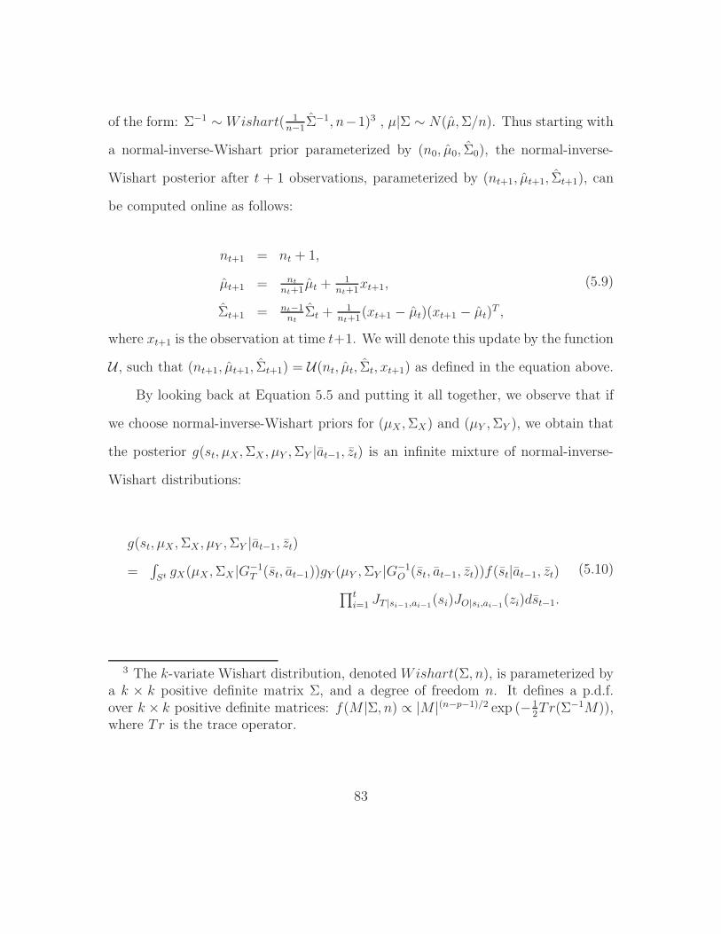
of the form: Σ−1 ∼Wishart( 1n−1

Σ−1, n−1)3 , µ|Σ ∼ N(µ,Σ/n). Thus starting with

a normal-inverse-Wishart prior parameterized by (n0, µ0, Σ0), the normal-inverse-

Wishart posterior after t + 1 observations, parameterized by (nt+1, µt+1, Σt+1), can

be computed online as follows:

nt+1 = nt + 1,

µt+1 = ntnt+1

µt +1

nt+1xt+1,

Σt+1 = nt−1nt

Σt +1

nt+1(xt+1 − µt)(xt+1 − µt)T ,

(5.9)

where xt+1 is the observation at time t+1. We will denote this update by the function

U , such that (nt+1, µt+1, Σt+1) = U(nt, µt, Σt, xt+1) as defined in the equation above.

By looking back at Equation 5.5 and putting it all together, we observe that if

we choose normal-inverse-Wishart priors for (µX ,ΣX) and (µY ,ΣY ), we obtain that

the posterior g(st, µX,ΣX , µY ,ΣY |at−1, zt) is an infinite mixture of normal-inverse-

Wishart distributions:

g(st, µX ,ΣX , µY ,ΣY |at−1, zt)

=∫

StgX(µX ,ΣX |G

−1T (st, at−1))gY (µY ,ΣY |G

−1O (st, at−1, zt))f(st|at−1, zt)

∏ti=1 JT |si−1,ai−1

(si)JO|si,ai−1(zi)dst−1.

(5.10)

3 The k-variate Wishart distribution, denoted Wishart(Σ, n), is parameterized bya k × k positive definite matrix Σ, and a degree of freedom n. It defines a p.d.f.over k × k positive definite matrices: f(M |Σ, n) ∝ |M |(n−p−1)/2 exp (−1

2Tr(Σ−1M)),

where Tr is the trace operator.

83

In practice, it will not be possible to compute exactly this posterior, but in

section 5.4 we present an algorithm that approximates this infinite mixture by a

finite mixture of normal-inverse-Wishart via Monte Carlo sampling. The essential

idea of this algorithm is that one can sample state sequences st, and for each such

sampled state sequence, maintain the normal-inverse-Wishart posteriors on the mean

and covariance of X and Y .

5.3 Bayes-Adaptive Continuous POMDP

We now consider the problem of optimal sequential decision-making in a con-

tinuous POMDP, as defined in Section 5.1, where the mean vectors and covariance

matrices of X and Y are the only unknown model parameters. To achieve this, we

proceed similarly to how the BAPOMDP model was defined (Section 4.2). First

notice that as in the BAPOMDP, if the agent could observe the state, it could

then maintain the exact normal-inverse-Wishart posteriors for X and Y (due to

the assumptions that GT |s,a and GO|s,a are invertible). However, due to the par-

tial observability of the state, the exact normal-inverse-Wishart posteriors for X

and Y are only partially observable through the observations z ∈ Z perceived by

the agent. Thus this decision problem can be represented as a problem of opti-

mal sequential decision-making under partial observability of both the state s ∈ S,

and normal-inverse-Wishart posteriors (ν, ω), where ν = (nX , µX , ΣX) represents the

normal-inverse-Wishart posterior parameters for X, and ω = (nY , µY , ΣY ) represents

the normal-inverse-Wishart posterior parameters for Y . Under such perspective, we

seek a policy that maps beliefs over tuples (s, ν, ω), to actions a ∈ A, such that it

maximizes expected long-term rewards of the agent. Similarly to the BAPOMDP,

84

we can define this problem as a Continuous POMDP over hyperstates (s, ν, ω), which

we call the Bayes-Adaptive Continuous POMDP (BACPOMDP).

The BACPOMDP is defined by the tuple (S ′, A′, Z ′, P ′, R′) where:

• S ′ = S×NWk×NW l, is the set of hyperstates, where NWk = {(n, µ, Σ)|n ∈

N+, µ ∈ R

k, Σ ∈ Rk2} is the space of normal-inverse-Wishart parameters over

k-dimensional multivariate Gaussian distributions.

• A′ = A, is the set of actions. This is the same as in the original continuous

POMDP, as we seek to find which actions in A the agent should choose.

• Z ′ = Z, is the set of observations. This is the same as in the original continuous

POMDP, as the agent gets the same observations.

• R′ is the reward function, such that R′(s, ν, ω, a) = R(s, a). The rewards are

defined as follows since we seek to optimize the rewards that are obtained in

the original continuous POMDP.

• P ′, is the joint transition-observation probability density function, such that

P ′(s, ν, ω, a, s′, ν ′, ω′, z) = f(s′, ν ′, ω′, z|s, ν, ω, a). Proceeding similarly to the

BAPOMDP, we can factorize this likelihood as:

f(s′, ν ′, ω′, z|s, ν, ω, a) = f(s′|s, ν, a)f(z|s′, ω, a)f(ν ′|s, a, s′, ν)f(ω′|s′, a, z, ω)

Here f(ν ′|s, a, s′, ν) = δ(ν ′ − U(ν,G−1T |s,a(s

′))) and f(ω′|s′, a, z, ω) = δ(ω′ −

U(ω,G−1O|s′,a(z))) are Dirac deltas4 which are non-zero only if ν ′ = U(ν,G−1

T |s,a(s′))

4 The Dirac delta is the probability measure of a random variable taking value0 with probability 1. It can be thought of as a p.d.f. where δ(x) = ∞I{0}(x) and

85

and ω′ = U(ω,G−1O|s′,a(z)) respectively, since the update of the normal-inverse-

Wishart posteriors is deterministic. Finally f(s′|s, ν, a) and f(z|s′, ω, a) can be

expressed by looking at the expectations of fX(G−1T |s,a(s

′)) and fY (G−1O|s′,a(z))

under the normal-inverse-Wishart posteriors ν and ω respectively, similarly to

the BAPOMDP, i.e.:

f(s′|s, ν, a) = JT |s,a(s′)

∫

fX(G−1T |s,a(s

′)|µX ,ΣX)f(µX ,ΣX |ν)d(µX ,ΣX),

f(z|s′, ω, a) = JO|s′,a(z)∫

fY (G−1O|s′,a(z)|µY ,ΣY )f(µY ,ΣY |ω)d(µY ,ΣY ).

However, here there are no simple closed-form solutions to these integrals.

In summary, the BACPOMPD, defined by the Continuous POMDP (S ′, A′, Z ′, P ′,

R′), has a known model and represents the decision problem of optimal sequential-

decision making in a continuous POMDP under both state and model uncertainty,

where model uncertainty is represented by normal-inverse-Wishart distributions.

If b0 ∈ ∆S is the initial belief of the original continuous POMDP, and ν0 ∈ NWk

and ω0 ∈ NW l are the normal-inverse-Wishart prior parameters, then the initial

belief of the BACPOMDP is defined by the p.d.f. b′0(s, ν, ω) = b0(s)δ(ν−ν0)δ(ω−ω0).

The model of the continuous POMDP is effectively learned by monitoring the belief

state of the BACPOMDP, which corresponds exactly to the posterior defined in

Equation 5.10.

Note that since the BACPOMDP is itself a Continuous POMDP, the belief

update and optimal value function equations defined in Equations 5.2 and 5.4 can

∫ ∞−∞ δ(x)dx = 1. Measure theory is essential to define it properly, but we leave out

such formalities since this it outside the scope of this thesis.

86

directly be used to monitor the belief of the BAPOMDP and compute its optimal

policy. However, as we can see, these equations are defined by complex integrals

which may not have a simple closed-form solution. In order to find an approximate

solution to the BACPOMDP, we propose to use Monte Carlo approximations of these

integrals. Hence, we first present a particle filter algorithm to approximate the belief

by a finite mixture of normal-inverse-Wishart distributions, and then an online Monte

Carlo planning algorithm which samples future sequences of actions and observations

in order to estimate the best immediate action to take in the environment.

5.4 Belief Monitoring

The particle filter algorithm presented in Algorithm 4 proceeds similarly to

the Monte Carlo particle filter for the BAPOMDP (Section 4.4). Starting from

the current belief b, represented by a set of K particles of the form (s, ν, ω), the

algorithm first samples a current hyperstate (s, ν, ω) according to the distribution

b. Then from this sampled current hyperstate, a next state s′ ∈ S is sampled

from f(s′|s, a, ν). This is achieved by sampling a mean µX and covariance ΣX

from the normal-inverse-Wishart posterior ν, then sampling the normal distribu-

tion N(µX ,ΣX) to obtain a value x for X, and finally evaluating the function

GT (s, a, x) to obtain s′, for the action a taken by the agent. This then allows us

to update the normal-inverse-Wishart posteriors by computing ν ′ = U(ν, x) and

ω′ = U(ω,G−1O|s′,a(z)). The last remaining part is to compute the weight of the

new particle (s′, ν ′, ω′) which is going to be added to the next belief b′. The like-

lihood of this particle should be proportional to f(z|s′, a, ω) for the observation z

87

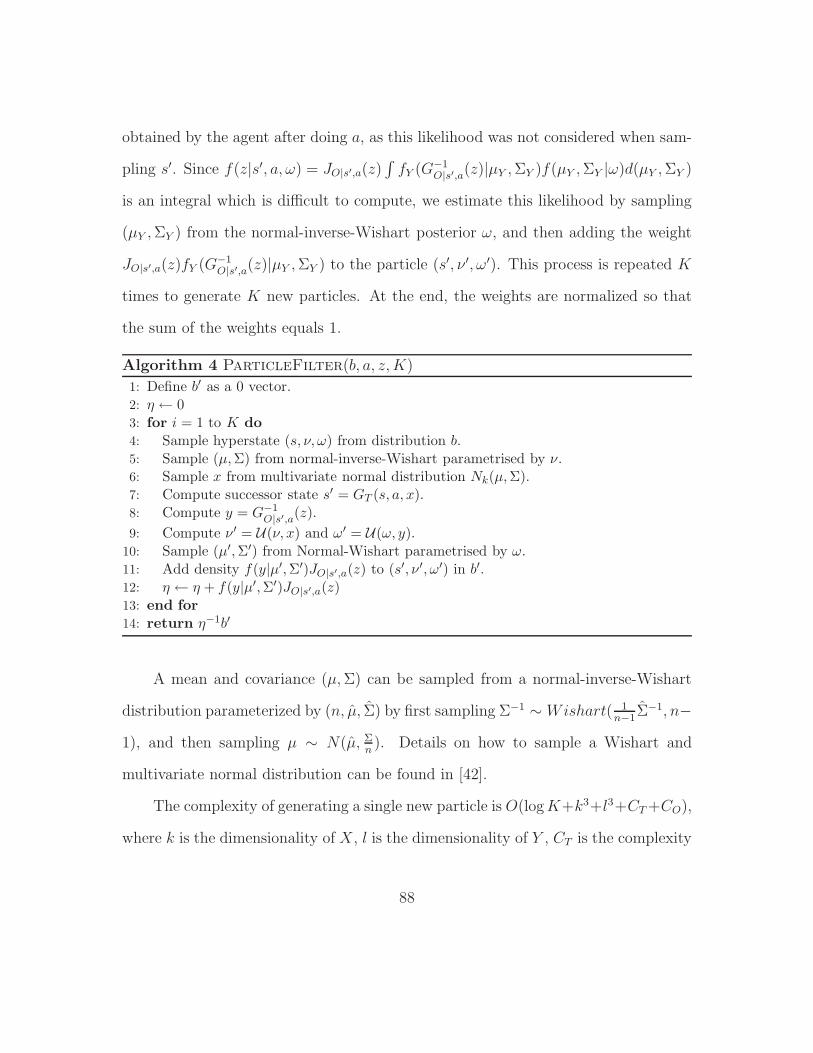
obtained by the agent after doing a, as this likelihood was not considered when sam-

pling s′. Since f(z|s′, a, ω) = JO|s′,a(z)∫

fY (G−1O|s′,a(z)|µY ,ΣY )f(µY ,ΣY |ω)d(µY ,ΣY )

is an integral which is difficult to compute, we estimate this likelihood by sampling

(µY ,ΣY ) from the normal-inverse-Wishart posterior ω, and then adding the weight

JO|s′,a(z)fY (G−1O|s′,a(z)|µY ,ΣY ) to the particle (s′, ν ′, ω′). This process is repeated K

times to generate K new particles. At the end, the weights are normalized so that

the sum of the weights equals 1.

Algorithm 4 ParticleFilter(b, a, z,K)

1: Define b′ as a 0 vector.2: η ← 03: for i = 1 to K do

4: Sample hyperstate (s, ν, ω) from distribution b.5: Sample (µ,Σ) from normal-inverse-Wishart parametrised by ν.6: Sample x from multivariate normal distribution Nk(µ,Σ).7: Compute successor state s′ = GT (s, a, x).8: Compute y = G−1

O|s′,a(z).9: Compute ν ′ = U(ν, x) and ω′ = U(ω, y).

10: Sample (µ′,Σ′) from Normal-Wishart parametrised by ω.11: Add density f(y|µ′,Σ′)JO|s′,a(z) to (s′, ν ′, ω′) in b′.12: η ← η + f(y|µ′,Σ′)JO|s′,a(z)13: end for

14: return η−1b′

A mean and covariance (µ,Σ) can be sampled from a normal-inverse-Wishart

distribution parameterized by (n, µ, Σ) by first sampling Σ−1 ∼ Wishart( 1n−1

Σ−1, n−

1), and then sampling µ ∼ N(µ, Σn). Details on how to sample a Wishart and

multivariate normal distribution can be found in [42].

The complexity of generating a single new particle is O(logK+k3+l3+CT+CO),

where k is the dimensionality of X, l is the dimensionality of Y , CT is the complexity

88

of evaluating GT (s, a, x) and CO is the complexity of evaluating G−1O|s′,a(z). Sampling

a hyperstate from b is O(logK), as b can be maintained as a cumulative distribution,

and the k3 and l3 complexity terms comes from the inversion of covariance matrices

and the sampling procedure for the normal-inverse-Wishart distribution. Hence per-

forming a belief update withK particles is achieved inO(K(logK+k3+l3+CT+CO)).

5.5 Online Planning

We now propose an approximate algorithm for planning in the BACPOMDP.

To ensure tractability, we focus on online methods for action selection, which means

that we try to find the optimal action (over a fixed planning horizon) for the cur-

rent belief state. Several online planning algorithms have been developed for finite

POMDPs (Section 2.2.2). Most of these require complete enumeration of the action

and observation spaces, which cannot be done in our continuous setting. For this

reason, we adopt a sampling-based approach [47, 50]. Algorithm 5 provides a brief

outline of the proposed online planning method.

At each time step, V (b,D,M,N,K) is executed with current belief b and then

action a is performed in the environment. The algorithm proceeds by recursively

expanding a tree of reachable beliefs by sampling uniformly a subset ofM actions and

a subset of N observations at each belief node, until it reaches a tree of depth D. The

particle filter is used to approximate the belief states. Sampling the observation from

f(z|b, a) is achieved similarly to how the particle filter works, i.e. from Algorithm

4: proceed with lines 4-7 to obtain a successsor state s′, then do line 10 to sample a

mean µ′ and covariance matrix Σ′ from the normal-inverse-Wisart posterior ω, draw

y from Nl(µ′,Σ′) and then the sampled observation is GO(s′, a, y). An approximate

89

Algorithm 5 V(b, d,M,N,K)

1: if d = 0 then

2: return V (b)3: end if

4: maxQ← −∞5: for i = 1 to M do

6: Sample a uniformly in A7: q ←

∑

(s,ν,ω) b(s, ν, ω)R(s, a)8: for j = 1 to N do

9: Sample z from f(z|b, a)10: b′ ← ParticleFilter(b, a, z,K)11: q ← q + γ

NV(b′, d− 1,M,N,K)12: end for

13: if q > maxQ then

14: maxQ← q

15: maxA← a

16: end if

17: end for

18: if d = D then

19: a← maxA

20: end if

21: return maxQ

value function V is used at the fringe node to approximate the value V ∗ of the fringe

beliefs. V can be obtained either from an approximate offline algorithm computing

an approximate value function of V ∗ or can simply be defined to 0 or the immediate

reward if we have no better estimate of the value function V ∗. The fringe nodes’

values are propagated to the parents’ nodes using an approximate version of Bellman

equation, where the maximization is taken over sampled actions, and expectation

over future rewards is taken over sampled observations. This yields a value estimate

for each sampled action at the current belief. The action with highest value estimate

is stored in the variable a. After executing a in the environment, the agent updates

its current belief b with the new observation z obtained using the particle filter. The

90

planning algorithm is then run again on this new belief to compute the next action

to take.

The overall complexity of this algorithm is in O((MN)D(Cp + Cv)), where Cp

denotes the complexity of doing the particle filter update, as given in the previous

section, and Cv denotes the complexity of evaluating the approximate value function

V . A nice property of our approach is that the complexity depends almost entirely

on user specified parameters, such that the parameters (M ,N ,D,K) can be adjusted

to meet problem specific real-time constraints.

Recent analysis has shown that it is possible to achieve ε-optimal performance

with an online POMDP planner [62] by using lower and upper bounds on V ∗ at the

fringe node. In our case, the use of sampling and particle filtering to track the belief

over state and model introduces additional error that prevents us from guaranteeing

lower and upper bounds. However, it may still be possible to guarantee ε-optimality

with high probability, provided that one chooses sufficiently large M ,N ,D and K

and that the value function is Lipschitz continuous. However this is non-trivial to

show and remains an open question for our particular framework.

5.6 Experimental Results

To validate our approach, we experimented on a simple simulated robot naviga-

tion problem where the simulated robot must learn the drift induced by its imperfect

actuators, and also the noise of its sensors. The robot moves in an obstacle-free

2D area and tries to reach a specific goal location. We define the state to be the

robot’s 2D cartesian position; actions are defined by (d, θ), where d ∈ [0, 1] relates

to the displacement and θ ∈ [0, 2π] is the angle toward which the robot moves; the

91

observations correspond to the robot’s position with additive Gaussian noise, i.e.

GO(s, a, y) = s+ y. The dynamics of the robot are assumed to be of the form:

GT (s, < d, θ >,X) = s+ d

cos θ − sin θ

sin θ cos θ

X.

The exact parameters of the normal distribution for X are the mean, µX = (0.8; 0.3),

and covariance ΣX = [0.04,−0.01;−0.01, 0.01]. Similarly, the observation noise,

Y , is parameterized by µY = (0; 0) and ΣY = [0.01, 0; 0, 0.01]. Both X and Y

must be estimated from data. The robot starts with the incorrect assumption that

for X, µX = (1, 0) and ΣX = [0.04, 0; 0, 0.16], and for Y , µY = (0; 0) and ΣY =

[0.16, 0; 0, 0.16]. The normal-inverse-Wishart prior parameters used for X are the

tuple ν0 = (10, µX, ΣX) and for Y , ω0 = (10, µY , ΣY ). This is equivalent to giving an

initial sample of 10 observations to the robot, in which the random variable X has

sample mean µX and sample covariance ΣX and the variable Y has sample mean µY

and sample covariance ΣY .

Initially the robot starts at the known position (0; 0), and the goal is a circular

area of radius 0.25 unit where the center position is randomly picked at a distance

of 5 units. As soon as the robot reaches a position inside the goal, a new goal center

position is chosen randomly (within a distance of 5 units from the previous goal).

The robot always knows the position of the current goal, and receives a reward of 1

when it reaches it. A discount factor γ = 0.85 is used.

For the planning, we assume a horizon of D = 1, and sample M = 10 ac-

tions, N = 5 observations and K = 100 particles to maintain the belief. The

92

0 50 100 150 200 2500

0.1

0.2

0.3

0.4

0.5

0.6

0.7

0.8

0.9

1

Training Steps

Ave

rage

Ret

urn

Prior modelExact ModelLearning

Figure 5–1: Average return as a function of the number of training steps.

approximate value function V at the planning fringe was computed as V (b) =

∑

(s,ν,ω) b(s, ν, ω)γG(s,ν), where G(s, ν) is the number of steps required to reach the

goal from s if the robot moves in a straight-line towards the goal with distance ||νµ||2

per step.

The average return as a function of the number of training episodes (averaged

over 1000 episodes) is plotted in Figure 5–1. We also compare it to the average

return obtained by planning only with the prior (with no learning), and planning

with the exact model, using the same parameters for M ,N ,D,K. As we can see, our

approach is able to quickly reach performance very close to the case where it was

given the exact model. Average running time for the planning was 0.074 seconds per

time step on an Intel Xeon 2.4Ghz processor.

To measure the accuracy of the learned model, we computed a weighted L1-

distance of the estimate (sample mean and sample covariance) in each particle com-

pared to the true model parameters as follows:

93

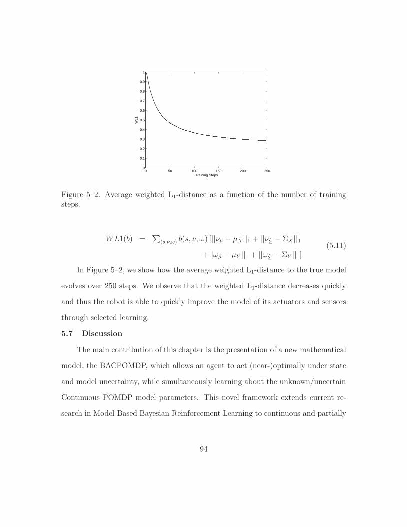
0 50 100 150 200 2500

0.1

0.2

0.3

0.4

0.5

0.6

0.7

0.8

0.9

1

Training Steps

WL1

Figure 5–2: Average weighted L1-distance as a function of the number of trainingsteps.

WL1(b) =∑

(s,ν,ω) b(s, ν, ω) [||νµ − µX ||1 + ||νΣ − ΣX ||1

+||ωµ − µY ||1 + ||ωΣ − ΣY ||1](5.11)

In Figure 5–2, we show how the average weighted L1-distance to the true model

evolves over 250 steps. We observe that the weighted L1-distance decreases quickly

and thus the robot is able to quickly improve the model of its actuators and sensors

through selected learning.

5.7 Discussion

The main contribution of this chapter is the presentation of a new mathematical

model, the BACPOMDP, which allows an agent to act (near-)optimally under state

and model uncertainty, while simultaneously learning about the unknown/uncertain

Continuous POMDP model parameters. This novel framework extends current re-

search in Model-Based Bayesian Reinforcement Learning to continuous and partially

94

observable domains. The main practical issue with this framework is the compu-

tational complexity of monitoring the belief state and planning the best action to

execute, which have no known closed-form solutions. Our proposed particle filter

algorithm for maintaining the belief and online Monte Carlo planning algorithm

provide a novel tractable approximate solution to the BACPOMDP that can be

computed in polynomial-time. This algorithmic solution allows a trade-off between

solution quality and computation time, which is achieved by changing the number

of particles K, the planning horizon D, the number of sampled actions M , and the

sampled observations N at each belief node in the planning tree. However, since the

planning tree grows exponentially in the planning horizon D, this approach is mostly

efficient in tasks requiring only a short planning horizon, unless a good approximate

value function V is used at the fringe.

It should be noted that there exists a large body of work in the control theory

literature that have tried to address a similar problem. The problem of optimal

control under uncertain model parameters was originally introduced by Feldbaum

[25], as the theory of dual control, also sometimes refered to as adaptive control

or adaptive dual control. Extensions of this theory has been developed for time-

varying systems [26]. Several authors have studied this problem for different kinds

of dynamical systems : linear time invariant systems under partial observability [64],

linear time varying Gaussian models under partial observability [61], nonlinear sys-

tems with full observability [82], and more recently a similar approach to ours, using

particle filters, has been proposed for nonlinear systems under partial observability

95

[33]. Our proposed approach differs from [33] in that we use normal-Wishart dis-

tributions to maintain the posterior, and use a different particle filtering algorithm.

Furthermore, their planning algorithm proceeds by evaluating a particular policy on

the underlying MDP defined by each particle, and then averaging the value of the

policy over all particles. Contrary to our approach, this does not reflect the value of

information gained by actions that help identify the state or the parameters of the

model, as it does not consider how the posterior distribution evolves in the future,

for different actions and observations.

Also note that in this chapter, it was assumed that the functions specifying the

dynamics GT and GO are known. This could be an important limitation in practice

as these may not be known. One possibility for future research is to generalize the

current BACPOMDP framework to handle cases where GT and GO are unknown.

We believe that Gaussian Processes could be used to define prior and posterior dis-

tributions over GT and GO. This would allow the agent to learn the full linear

or nonlinear dynamics of the system, without any particular parametric assump-

tion (other than that the noise is Gaussian distributed) [23]. Other non-parametric

bayesian methods could also be investigated to learn the distributions f(s′|s, a) and

f(z|s′, a). Finally, more expressive parametric models could be investigated, such as

a mixture of Gaussians, which could also be learned via a Bayesian approach.

96

CHAPTER 6

Bayesian Reinforcement Learning in Structured Domains

Due to the high complexity of model-based BRL, most approaches based on

the BAMDP and BAPOMDP frameworks presented in Chapters 3 and 4 have been

limited to very small domains (less than a hundred states). This is mainly due to

two reasons. First, the number of parameters to learn grows quadratically in the

number of states, such that when the number of states is large, a large amount of

data needs to be collected to learn a good model (as with any tabular RL algorithm),

unless very few parameters are unknown or some structural assumptions are made

to represent the dynamics with few parameters. Second, most planning approaches

in model-based BRL become intractable as the number of states increases, since

planning is done over the full space of possible posteriors.

We seek to address these issues by proposing an extension of model-based BRL

to structured domains, which can exploit underlying structures that may exist in

the system in order to learn more efficiently the dynamics of the system in large do-

mains. Hence, we propose learning a factored representation of the dynamics via a

Bayesian approach. Factored representations can efficiently represent the dynamics

of a system with fewer parameters using a dynamic Bayesian network (DBN) that

exploits conditional independence relations existing between state features [5, 35].

Current model-based BRL techniques can be extended quite easily to factored rep-

resentations when the structure of this DBN is known, however this is unreasonable

97

in many domains. Fortunately, the problem of simultaneously learning the structure

and parameters of a Bayes Net has received some attention [39, 28, 21], which we

can leverage in this chapter. However while these approaches provide an effective

way of learning the model, it is far from sufficient for model-based BRL, where the

goal is to choose actions in an optimal way, with respect to the full posterior over

models. To address the issue of action selection, we propose incorporating an online

Monte Carlo approach to evaluate sequences of actions with respect to the posterior

over structures and parameters, similar to the proposed online planning algorithms

for the BAPOMDP (Section 4.5) and BACPOMDP (Section 5.5).

In this chapter, background on Bayesian Networks (BNs) and bayesian learning

algorithms for BNs are first introduced. Then we show how such BNs can be used

to represent an MDP more compactly in factored form. Afterwards, we show how

these compact factored respresentations can be leveraged in a model-based BRL

framework. One issue is that the posterior over DBN structures is intractable to

maintain in practice. To overcome this problem, an MCMC algorithm is used to

periodically resample structures from this posterior. Finally, an online planning

algorithm is presented to find an approximate solution to the problem of optimal

sequential-decision making under both structure and parameter uncertainty. Note

that in this chapter we focus entirely on fully observable domains (i.e. MDPs),

but the proposed approach should extend easily to partially observable domains by

combining with the work presented in Chapter 4.

98

6.1 Structured Representations

In this section, we introduce some background on Bayesian Networks and how

such structure can be learned from observations via a bayesian method. We then

present the factored MDP model, which uses Dynamic Bayesian Networks to repre-

sent compactly the dynamics of an MDP.

6.1.1 Learning Bayesian Networks

Bayesian networks (BNs) have been used extensively to build compact predictive

models of multivariate data [56]. A BN models the joint distribution of multivariate

data compactly by exploiting conditional independence relations between variables.

It is defined by a set of variables X = (X1, . . . , Xn), a directed acyclic graph (DAG)

structure G over variables in X, and parameters θG, where θi,v|EG specifies the proba-

bility that Xi = v given that its parents in G take value E (E is a vector assigning a

value to each parent of Xi). We denote Xi, the set of possible values for variable Xi,

XG≺i the set of parents’ variables of variable Xi in structure G, XG

≺i =∏

Xj∈XG≺iXj

the set of possible parents’ values for variable Xi.

Several approaches exist to learn BNs. Learning a Bayes net can involve either

only learning θG (if the structure G is known), or simultaneously learning the struc-

ture G and parameters θG. For our purposes, we are mostly interested in Bayesian

approaches that learn both the structure and parameters [39, 28, 21]. These Bayesian

approaches proceed by first specifying a joint prior, g(G, θG), of the form:

g(G, θG) = g(G)g(θG|G), (6.1)

99

where g(G) is a prior over structures and g(θG|G) is a conditional prior on the

parameters θG given a particular structure G. g(G) is often chosen to be uniform,

or proportional to β |E(G)| for some β ∈ (0, 1) where |E(G)| is the number of edges in

G, such as to favor simpler structures.

It follows that if dataset D is observed, then the joint posterior is defined as

follows:

g(G, θG|D) = g(G|D)g(θG|G,D). (6.2)

To compute this posterior efficiently, several assumptions are usually made about

the prior g(θG|G). First, it should factorize into a product of independent Dirichlet

priors:

g(θG|G) =∏n

i=1

∏

E∈XG≺ig(θ

i,·|EG |G),

g(θi,·|EG |G) ∼ Dirichlet(φ

i,·|EG ),

(6.3)

where φi,v|EG represents the prior Dirichlet count parameter for the observation of

Xi = v given XG≺i = E. Under this independence assumption, the term g(θG|G,D)

is a product of Dirichlet distributions, which can be updated easily by incrementing

the counts φi,v|EG by one for each observation of (Xi, X

G≺i) = (v, E) in D. Hence if

φG denotes the current Dirichlet count parameters, and a new observation X = x is

obtained, the posterior Dirichlet count parameters φ′G after observation of X = x,

can be updated via the following update rule:

φ′i,xi|xG≺iG = φ

i,xi|xG≺iG + 1 ∀i ∈ 1, . . . , n

φ′i,v|EG = φ

i,v|EG ∀i ∈ 1, . . . , n, (v, E) ∈ (Xi × XG

≺i)− {(xi, xG≺i)},

(6.4)

100

where xi denotes the value of variable Xi in observation x, xG≺i the values of the

parents of Xi in structure G for the observation x. We denote this update rule by

the function U , such that φ′G = U(φG, x) as defined in the previous equation.

A second common assumption is that two equivalent graph structures G and

G′ should have equivalent priors over θG and θ′G (this is called the likelihood equiv-

alence assumption). This enforces a strong relation between the priors g(θG|G) and

g(θGc|Gc) for the complete graph Gc (where every variable depends on all previ-

ous variables), such that specifying φGc totally specifies the prior on θG for any

other graph G (i.e. for any graph G, the prior Dirichlet count parameters satisfy

φi,v|EG = N Pr(Xi = v,XG

≺i = E|Gc, φGc) where N =∑

E∈XGc≺i

∑

v∈Xi φi,v|EGc

is the

equivalent sample size for the prior on θGc).

For many problems, the posterior g(G|D) cannot be maintained in closed form

as it corresponds to a discrete distribution over O(n!2(n2)) possible graph structures.

Instead, MCMC algorithms can be used to sample graph structures from this poste-

rior [28]. The well known Metropolis-Hasting algorithm specifies that a move from

graph G to G′ should be accepted with probability min{

1, f(D|G′)g(G′)q(G|G′)f(D|G)g(G)q(G′ |G)

}

, where

q(G′|G) is the probability that a move from G to G′ is proposed and f(D|G) =∫

f(D|G, θG)g(θG|G)dθG is the likelihood of the dataset D given the graph G. Such

random walk in the space of DAGs has the desired stationary distribution g(G|D).

Under previous assumptions concerning the prior g(θG|G), g(D|G) can be computed

in closed form and corresponds to the Bayesian Dirichlet likelihood equivalent metric

(BDe) [39]:

101

g(D|G) =

n∏

i=1

∏

E∈XG≺i

Γ(∑

v∈Xi φi,v|EG )

Γ(∑

v∈Xi φ′i,v|EG )

∏

v∈Xi

Γ(φ′i,v|EG )

Γ(φi,v|EG )

, (6.5)

where φG represents the prior counts before the observation of dataset D, and φ′G

the posterior counts after the observation of D (i.e. φ′G is obtained by recursively

applying the function U for each datapoint x ∈ D, starting from φG).

Typical moves considered in the MCMC algorithm include adding an edge, delet-

ing an edge, or reversing an edge in G. For faster mixing in the space of DAGs, some

recent approaches first sample a topological order for G and then perform addition

and deletion of edges in G for the fixed sampled topological order [28].

6.1.2 Factored MDPs

Dynamic Bayesian Networks (DBNs) can be used to represent MDPs in a more

compact form by exploiting conditional independence relations that exist between

state features. A DBN is essentially a bayesian network with a notion of time built

into it, i.e. we are interested in expressing compactly the joint distribution of the

variables (Xt,1, . . . , Xt,n) at time t given variables (Xt−1,1, . . . , Xt−1,n) at time t−1 by

exploiting conditional independence relations that may exist between these variables.

A factored MDP is an MDP where the state is described by a set of state features

(or state variables) and its transition function is specified via a DBN. It is formally

defined by a tuple (S,A, T,R):

• S : S1 × S2 × · · · × Sn, is the (discrete) set of states of the system; S1, . . . , Sn

correspond to the domain of the n state variables (features).

• A, the (discrete) set of actions that can be performed by the agent.

102

• T : S × A × S → [0, 1], the transition function, where T (s, a, s′) = Pr(s′|s, a)

represents the probability of moving to state s′ if the agent executes action a

in state s. This can be represented efficiently using a seperate DBN for each

action, thus exploiting conditional independence relations that exist between

state features [5]. For simplicity, we assume that these DBNs are bipartite

graphs, so dependencies only exist between state variables at time t and state

variables at time t+ 1.

• R : S × A → R, the reward function, defined for every action of the agent in

every state.

The DBN defining T for any action a ∈ A is represented by a graph G(a) and set of

parameters θG(a) defining the conditional probability tables. We denote s′i the next

state’s ith feature, si the current state’s ith feature, Si the set of possible values for si

and s′i, sG≺i the values of the parents’ features of s′i in s for graph G, and SG≺i the set

of possible values for the parents’ features of s′i for graph G. For each possible value

v ∈ Si of next state variable s′i, and each possible assignment to its parent values

E ∈ SG(a)≺i , θG(a) contains a parameter θ

i,v|EG(a) that defines Pr(s′i = v|sG(a)

≺i = E, a).

Given such graph G(a) and parameters θG(a), T (s, a, s′) is computed efficiently as:

T (s, a, s′) =

n∏

i=1

Pr(s′i|sG(a)≺i , a). (6.6)

The optimal value function and policy of a factored MDP is defined as for the stan-

dard (non-factored) MDP, as shown in Section 2.1.1. In general, a factored represen-

tation of the transition does not induce a structured representation of the optimal

103

value function. However, approximate algorithms exist to compute V ∗ more effi-

ciently by exploiting the factored representation [35].

6.2 Structured Model-Based Bayesian Reinforcement Learning

Now that we have shown how the transition function of an MDP can be defined

compactly via a set of DBNs, and how the structure and parameters of a DBN can

be learned via a bayesian approach, we can address the problem of acting optimally

in a system represented as a factored MDP, in the case where both the structure

and parameters of the DBNs defining the transition function, T , are unknown. It is

assumed that the state features S1, . . . , Sn, the action set A, and the reward function

R, are known.

In order to formulate this as a sequential decision problem, we consider the

transition function T as a hidden variable of the system, which is partially observed

through the state transitions that occur in the system. In this view, the decision

problem can be cast as a POMDP (Section 2.2). The hyperstates of this POMDP

capture both the known current system state, and the hidden DBN structures and

parameters defining T for each action a ∈ A. Formally, this POMDP is defined by

the tuple (S ′, A′, Z ′, T ′, O′, R′):

• S ′ : S × G|A|, where S is the original state space of the MDP, G is the set of

DBNs (G, θG) (one per action) and G is a bipartite graph from S1, . . . , Sn to

S1, . . . , Sn.

• A′ = A, the set of actions in the original MDP.

• Z ′ = S, the set of observations (i.e a transition to a particular state of the

MDP).

104

• T ′ : S ′ ×A′ × S ′ → [0,∞], the transition function in this POMDP:

T ′(s,G, θG, a, s′, G′, θ′G′)

= f(s′, G′, θ′G′ |s,G, θG, a)

= Pr(s′|s,G, θG, a)f(G′, θ′G′ |G, θG, s, a, s′),

(6.7)

where G = {G(a)|a ∈ A}, θG = {θG(a)|a ∈ A}, and similarly for G′ and θG′ .

Since we assume that the transition function T does not change over time,

then f(G′, θ′G′|G, θG, s, a, s′) =∏

a′∈A IG(a′)(G′(a′))δ(θG(a′) − θ′G′(a′)) (i.e. with

probability 1, (G′, θ′G′) = (G, θG)), and Pr(s′|s,G, θG, a) =∏n

i=1 θi,s′i|s

G(a)≺i

G(a) , so

that∑

s′,G′

∫

T ′(s,G, θG, a, s′, G′, θ′G′)dθ′G′ = 1.

• O′ : S ′ × A′ × Z ′ → [0, 1], the observation function, where O(s′, G′, θ′G′, a, z) is

the probability of observing z when moving to (s′, G′, θ′G′) by doing action a.

Here, the agent simply observes the state of the MDP, so O(s′, G′, θ′G′ , a, z) =

I{s′}(z).

• R′ : S ′ × A′ → R, the reward function, which corresponds directly to the

rewards obtained in the MDP, i.e. R′(s,G, θG, a) = R(s, a).

Given that the hyperstate is not directly observable (i.e. we do not know the correct

structure and parameters), we maintain a probability distribution over states, called

a belief. The initial belief state in this POMDP is the initial state of the environment,

along with priors P (G(a), θG(a)), ∀a ∈ A. At time t, the belief state corresponds to

the current state of the MDP, st, along with posteriors P (G(a), θG(a)|st, at−1), ∀a ∈ A,

where st and at−1 are the histories of visited states and actions respectively at time

t.

105

To represent this belief compactly, we assume that the joint priors g(G(a), θG(a))

satisfy the assumptions stated in section 6.1.1, namely they factorize into a product

g(G(a), θG(a)) = g(G(a))g(θG(a)|G(a)) and the g(θG(a)|G(a)) terms are defined by a

product of independent Dirichlet distributions. For each graph G(a), starting from

prior counts φi,v|EG(a) for all state variables s′i, values v ∈ Si, and parent values E ∈ SG(a)

≺i ,

the posterior counts are maintained by simply incrementing by 1 the counts φi,s′i|s

G(a)≺i

G(a)

for all state variables s′i, each time a transition (s, a, s′) occurs. As mentioned in

section 6.1.1, the main difficulty is in maintaining the posterior g(G(a)|st, at−1) at

any time t, which is infeasible when the space of graphs is large. We approximate this

using a particle filter, and for each particle (i.e. a sampled graph G(a)), the posterior

g(θG(a)|G(a), st, at−1) is maintained exactly with counts φG(a). This particle filter is

explained in more detail in the next section.

Finding the optimal policy for this POMDP yields an action selection strat-

egy that optimally trades-off between exploration and exploitation such as to max-

imize long term expected return given the current model posterior and state of the

agent. Our structured model-based BRL approach therefore requires solving this

POMDP. While many algorithms exist to solve POMDPs, few of them can handle

high-dimensional infinite state spaces, as is required here. Hence, in Section 6.4, we

propose to use online Monte Carlo methods to solve this challenging optimization

problem [50], similarly to the planning techniques proposed in Chapter 4 and 5.

6.3 Belief Monitoring

As mentioned above, for each a ∈ A, the posterior g(G(a)|st, at−1) is maintained

using a particle filter algorithm. This is achieved by keeping a fixed set of K sampled

106

graph structures {G(a, j)|j ∈ {1, . . . , K}} and maintaining for each sampled graph

G(a, j) a probability pja. For each sampled graph G(a, j), we also maintain the

Dirichlet posterior count parameters φG(a,j) on the parameters θG(a,j). The graphs

G(a, j) are initially sampled from the prior Pr(G(a)).

Whenever a transition (s, a, s′) occurs, the probability pja of graph G(a, j) is

updated as follows:

p′ja = 1ηpja

∫

Pr(s′|s, a, G(a, j), θG(a,j))f(θG(a,j)|G(a, j), φG(a,j))dθG(a,j),

= 1ηpja

∏ni=1

[

φi,s′i|s

G(a,j)≺i

G(a,j)/∑

v∈Si φi,v|sG(a,j)

≺i

G(a,j)

]

,(6.8)

where the integral term is just the expected probability of Pr(s′|s, a) under the

current posterior for θG(a,j), defined by the counts φG(a,j), and η is a normalization

constant such that∑K

j=1 p′ja = 1. After the probability of each graph has been

updated, the Dirichlet posteriors are updated for each sampled graph G(a, j) by

incrementing the appropriate counts in φG(a,j) for the transition (s, a, s′):

φ′i,s′i|s

G(a,j)≺i

G(a,j)= φ

i,s′i|sG(a,j)≺i

G(a,j)+ 1 ∀i ∈ {1, . . . , n}

φ′i,v|EG(a,j)

= φi,v|EG(a,j)

∀i ∈ {1, . . . , n}, (v, E) ∈ (Si × SG(a,j)≺i )− {(s′i, s

G(a,j)≺i )},

(6.9)

where φ′G(a,j)

represents the posterior counts for sampled graph G(a, j) after the

observation of (s, a, s′).

These two procedures allow us to (approximately) maintain the posterior over

structure (by maintaining it over a subset of graphs), and (exactly) maintain the

posterior over the probability parameters of each sampled graph via the Dirichlet

107

count parameters. However this is insufficient to learn the correct DBN structure

defining T for each action a ∈ A. In particular, if the correct structures are not

among the sampled structures, then it will be impossible to learn the correct ones

by just ajusting the probability of each sampled structure.

We address this problem by periodically resampling a new set of DBN structures

from the current posterior P (G(a)|st, at−1) to obtain more likely structures after

observation of the history of states st and history of actions at−1. We implement

this by using an MCMC algorithm, as described in Section 6.1.1. Note that in our

case, the DBNs representing T have a known order since they are assumed to be

bipartite graphs (i.e. variables si always precede any of the variables s′j). Hence,

sampling orders is not required for our purposes. Furthermore, since we cannot have

any variable si depend on any next state variable s′j , we do not consider moves that

inverse an edge in the MCMC algorithm. Thus our MCMC algorithm only proposes

moves which add an edge between a current state feature si to a next state feature

s′j, or delete a currently existing edge.

In general, it may not be appropriate to resample graphs too frequently. One

useful criteria to decide when to resample new graphs is to look at the overall likeli-

hood La of the current set of DBNs for a particular action a. This can be computed

directly from the normalization constant η (Equation 6.8). Presuming that at time

t = 0, La = 1, we can simply update L′a = ηLa at every step where action a is taken.

Then if at time t, La falls below some predefined threshold, we resample a new set

of K graph structures G′(a, j) from posterior g(G(a)|st, at−1) and update the Dirich-

let posterior g(θG(a,j)|G(a, j), st, at−1) for each graph according to the whole history

108

(st, at−1) (starting from the Dirichlet prior g(θG(a)|G(a))). The probabilities pja for

these new graphs are then reinitialized to 1K

and the likelihood La to 1.

6.4 Online Planning

Turning our attention to the planning problem, we now search for the best action

to execute, given the current state, the current distribution on sampled graphs for

each action a (defined by pja), and the current posterior over parameters for each

sampled graph. Define Q∗(s, b, a) to be the maximum expected sum of rewards (i.e.

the value) of applying action a when the agent is in MDP state s and has posterior b

over DBNs. Then the optimal value is defined by V ∗(s, b) = maxa∈AQ∗(s, b, a) and

the best action to apply is simply arg maxa∈AQ∗(s, b, a).

Algorithm 6 V(s, b, d, N)

1: if d = 0 then

2: return V (s, b)3: end if

4: maxQ← −∞5: for a ∈ A do

6: q ← R(s, a)7: for j = 1 to N do

8: Sample s′ from Pr(s′|s, b, a)9: b′ ← UpdateGraphPosterior(b, s, a, s′)

10: q ← q + γNV(s′, b′, d− 1, N)

11: end for

12: if q > maxQ then

13: maxQ← q

14: maxA← a

15: end if

16: end for

17: if d = D then

18: a← maxA

19: end if

20: return maxQ

109

A recursive approach for tractably estimating V ∗(s, b) using a depth-limited

online Monte Carlo search is provided in Algorithm 6. Every time the agent needs

to execute an action, the function V(s, b,D,N) is called for the current state s and

posterior b. D corresponds to the depth of the search tree (i.e. planning horizon) and

N to the branching factor (i.e. number of successor states to sample at each level, for

each action). To sample a successor state s′ from P (s′|s, b, a), we can simply pick one

of the sampled graphs G(a, j) for action a according to the probabilities pja and then

sample s′ from this DBN, given that the parents take values s. At the fringe of the

planning tree, an estimate V (s, b) of the return obtained from this posterior is used.

Several techniques can be used to estimate V (s, b). For instance one could maintain

an approximate value function Vj(s) for each sampled factored MDP defined by the

DBNs {(G(a, j), φG(a,j))|a ∈ A} and then compute V (s, b) =∑K

j=1 Vj(s)∏

a∈A pja.

The approximate value functions Vj(s) can be updated efficiently via prioritized

sweeping every time the counts φG(a,j) are updated. For the experiments presented

below, we simply use V (s, b) = maxa∈AR(s, a). The UpdateGraphPosterior

updates the Dirichlet posteriors and probabilities pja presuming a transition (s, a, s′)

was observed, as defined in Equations 6.8 and 6.9. The best action to execute

for the current time-step can be retrieved through the a variable set during the

online planning algorithm. The computation time allowed to estimate V ∗(s, b) can be

limited by controlling the branching factor (N), search depth (D), and the number of

sampled graph structures (K) for each action, albeit at the expense of lesser accuracy.

110

6.5 Experimental Results

To validate our approach, we experiment with instances of the network adminis-

tration domain [35]. A network is composed of n computers linked together by some

topology. Each computer is either in running or failure mode. A running computer

has some probability of transitioning to failure, independent of its neighbors in the

network; that probability is increased for every neighbor in failure mode. A com-

puter in failure mode remains so until rebooted by the operator. A reward of +1

is obtained for every running computer in the network at every step. No reward is

given for failed computers, and a −1 reward is received for each rebooting action.

The goal of the operator is to maximize the number of running computers while

minimizing reboots actions. The starting state assumes all computers are running.

In our experiments, we assume a probability 130

that a running computer goes

into failed mode and a probability 110

that a failed computer induces failure in any

of its neighbors. So at any step, the probability that a running computer remains in

a running state is 2930

(0.9)NF where NF is the number of neighbors in failure state.

We assume a discount factor γ = 0.95.

This problem can be modeled by a factored MDP with n binary state variables,

each representing the running state of a computer in the network. There are n + 1

actions: one reboot action for each computer and a DoNothing action. The DBN

structure representing the dynamics when no reboot is performed is a bipartite graph

where the state variable s′i (the next state of computer i) depends on si (the previous

state of computer i) and sj for all computers j connected to i in the network. Note

that if s′i depends on sj, then this implies j is connected to i and thus s′j depends on

111

si. Hence the adjacency matrix A encoding the dependence relations in this bipartite

graph (where entry Aij = 1 if s′j depend on si, 0 otherwise) is always symmetric and

has a main diagonal full of ones.

In terms of prior knowledge, we assume the agent knows that rebooting a com-

puter always puts it back into running mode and does not affect any other computer.

The goal of the agent is to learn the behavior of each computer in the network when

no reboot is performed on them. Therefore, a single DBN is learned for the behavior

of the system when no reboot is performed. We also assume the agent knows that

the adjacency matrix is symmetric and has a main diagonal of ones. However we do

not assume that the agent knows the topology of the network. We choose a prior

over structures that is a uniform distribution over bipartite graphs with symmetric

adjacency matrix (and main diagonal equal to 1). Given a prior of this form, the

set of moves we consider to sample graphs in the Metropolis-Hasting algorithm con-

sists of inverting any of the binary variables in the upper-right half of the adjacency

matrix A (excluding the main diagonal) as well as the corresponding entry in the

bottom-left half. Moves of this type preserve the symmetry in the adjacency matrix,

and correspond to adding or removing a connection between any pair of computers

in the network. We assume no prior knowledge regarding the probabilities of failure,

so a uniform Dirichlet prior is used. Under the likelihood equivalence assumption,

the prior counts φG are defined such that φi,v|EG = 1

|SG≺i||Si|.

We consider three different network architectures: a simple linear network of

10 computers (1024 states), a ternary tree network composed of 13 computers (8192

112

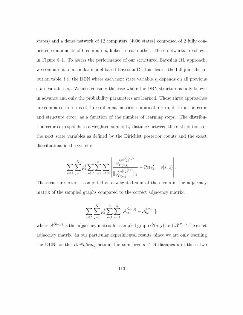
states) and a dense network of 12 computers (4096 states) composed of 2 fully con-

nected components of 6 computers, linked to each other. These networks are shown

in Figure 6–1. To assess the performance of our structured Bayesian RL approach,

we compare it to a similar model-based Bayesian RL that learns the full joint distri-

bution table, i.e. the DBN where each next state variable s′i depends on all previous

state variables sj. We also consider the case where the DBN structure is fully known

in advance and only the probability parameters are learned. These three approaches

are compared in terms of three different metrics: empirical return, distribution error

and structure error, as a function of the number of learning steps. The distribu-

tion error corresponds to a weighted sum of L1-distance between the distributions of

the next state variables as defined by the Dirichlet posterior counts and the exact

distributions in the system:

∑

a∈A

K∑

j=1

pja∑

s∈S

n∑

i=1

∑

v∈Si

∣

∣

∣

∣

∣

∣

∣

φi,v|sG(a,j)

≺i

G(a,j)

||φi,∗|sG(a,j)

≺i

G(a,j)||1

− Pr(s′i = v|s, a)

∣

∣

∣

∣

∣

∣

∣

.

The structure error is computed as a weighted sum of the errors in the adjacency

matrix of the sampled graphs compared to the correct adjacency matrix:

∑

a∈A

K∑

j=1

pja

n∑

i=1

n∑

k=1

|AG(a,j)ik −AG

∗(a)ik |,

where AG(a,j) is the adjacency matrix for sampled graph G(a, j) and AG∗(a) the exact

adjacency matrix. In our particular experimental results, since we are only learning

the DBN for the DoNothing action, the sum over a ∈ A dissapears in those two

113

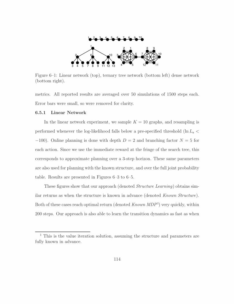
1 2 3 4 5 6 7 8 9 10

1

2 6 10

3 4 5 7 8 9 11 12 13

12

3

4 5

6 7

8 9

10

1112

Figure 6–1: Linear network (top), ternary tree network (bottom left) dense network(bottom right).

metrics. All reported results are averaged over 50 simulations of 1500 steps each.

Error bars were small, so were removed for clarity.

6.5.1 Linear Network

In the linear network experiment, we sample K = 10 graphs, and resampling is

performed whenever the log-likelihood falls below a pre-specified threshold (lnLa <

−100). Online planning is done with depth D = 2 and branching factor N = 5 for

each action. Since we use the immediate reward at the fringe of the search tree, this

corresponds to approximate planning over a 3-step horizon. These same parameters

are also used for planning with the known structure, and over the full joint probability

table. Results are presented in Figures 6–3 to 6–5.

These figures show that our approach (denoted Structure Learning) obtains sim-

ilar returns as when the structure is known in advance (denoted Known Structure).

Both of these cases reach optimal return (denoted Known MDP1) very quickly, within

200 steps. Our approach is also able to learn the transition dynamics as fast as when

1 This is the value iteration solution, assuming the structure and parameters arefully known in advance.

114

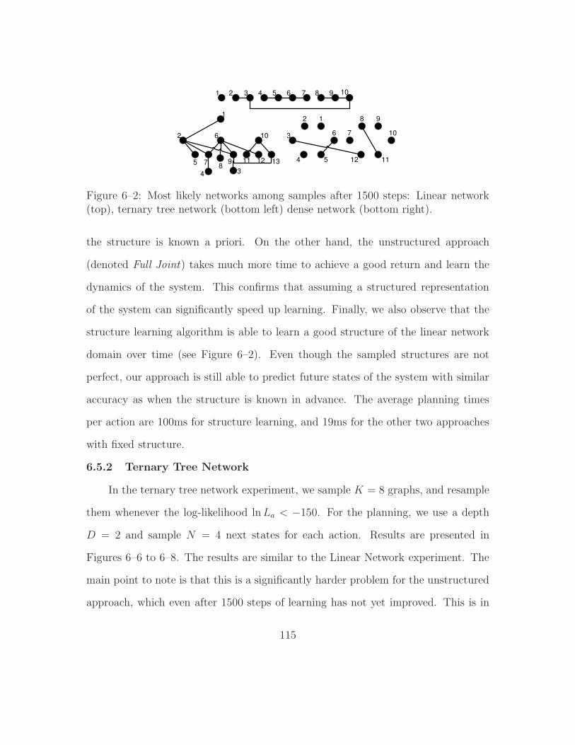
1 2 3 4 5 6 7 8 9 10

1

2 6 10

34

5 78

9 11 12 13

12

3

4 5

6 7

8 9

10

1112

Figure 6–2: Most likely networks among samples after 1500 steps: Linear network(top), ternary tree network (bottom left) dense network (bottom right).

the structure is known a priori. On the other hand, the unstructured approach

(denoted Full Joint) takes much more time to achieve a good return and learn the

dynamics of the system. This confirms that assuming a structured representation

of the system can significantly speed up learning. Finally, we also observe that the

structure learning algorithm is able to learn a good structure of the linear network

domain over time (see Figure 6–2). Even though the sampled structures are not

perfect, our approach is still able to predict future states of the system with similar

accuracy as when the structure is known in advance. The average planning times

per action are 100ms for structure learning, and 19ms for the other two approaches

with fixed structure.

6.5.2 Ternary Tree Network

In the ternary tree network experiment, we sample K = 8 graphs, and resample

them whenever the log-likelihood lnLa < −150. For the planning, we use a depth

D = 2 and sample N = 4 next states for each action. Results are presented in

Figures 6–6 to 6–8. The results are similar to the Linear Network experiment. The

main point to note is that this is a significantly harder problem for the unstructured

approach, which even after 1500 steps of learning has not yet improved. This is in

115

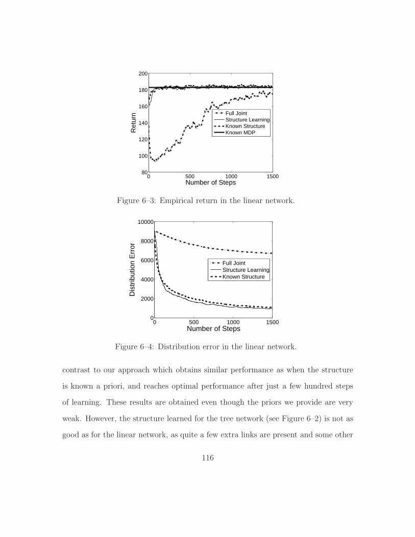
0 500 1000 150080

100

120

140

160

180

200

Number of Steps

Ret

urn Full Joint

Structure LearningKnown StructureKnown MDP

Figure 6–3: Empirical return in the linear network.

0 500 1000 15000

2000

4000

6000

8000

10000

Number of Steps

Dis

trib

utio

n E

rror

Full JointStructure LearningKnown Structure

Figure 6–4: Distribution error in the linear network.

contrast to our approach which obtains similar performance as when the structure

is known a priori, and reaches optimal performance after just a few hundred steps

of learning. These results are obtained even though the priors we provide are very

weak. However, the structure learned for the tree network (see Figure 6–2) is not as

good as for the linear network, as quite a few extra links are present and some other

116

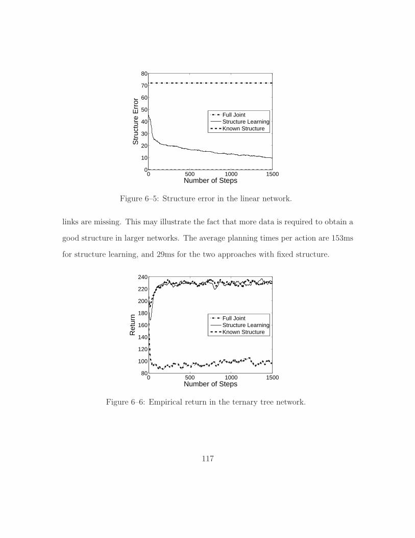
0 500 1000 15000

10

20

30

40

50

60

70

80

Number of Steps

Str

uctu

re E

rror

Full JointStructure LearningKnown Structure

Figure 6–5: Structure error in the linear network.

links are missing. This may illustrate the fact that more data is required to obtain a

good structure in larger networks. The average planning times per action are 153ms

for structure learning, and 29ms for the two approaches with fixed structure.

0 500 1000 150080

100

120

140

160

180

200

220

240

Number of Steps

Ret

urn Full JointStructure LearningKnown Structure

Figure 6–6: Empirical return in the ternary tree network.

117

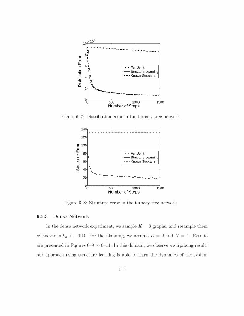
0 500 1000 15000

2

4

6

8

10x 10

4

Number of Steps

Dis

trib

utio

n E

rror

Full JointStructure LearningKnown Structure

Figure 6–7: Distribution error in the ternary tree network.

0 500 1000 15000

20

40

60

80

100

120

140

Number of Steps

Str

uctu

re E

rror

Full JointStructure LearningKnown Structure

Figure 6–8: Structure error in the ternary tree network.

6.5.3 Dense Network

In the dense network experiment, we sample K = 8 graphs, and resample them

whenever lnLa < −120. For the planning, we assume D = 2 and N = 4. Results

are presented in Figures 6–9 to 6–11. In this domain, we observe a surprising result:

our approach using structure learning is able to learn the dynamics of the system

118

much faster than when the structure is known in advance (see Figure 6–10), even

though the learned structures are still far from correct (see Figures 6–11 and 6–2).

This is a domain where there are many dependencies between state variables, so

there are many parameters to learn (whether or not the structure is known). In such

a case, our structure learning approach is at an advantage, because early on in the

learning, it can favor simpler structures which approximate the dynamics reasonably

well from very few learning samples (e.g. < 250). As further data is acquired,

more complex structures can be inferred (and more parameters estimated), in which

case our approach achieves similar return as when the structure is known, while it

continues to estimate the true parameters more accurately.

This result has important implications for RL in large domains. Namely, it

suggests that even in domains where significant dependencies exist between state

variables, or where there is no apparent structure, a structure learning approach can

be better than assuming a known (correct) structure, as it will find simple models

that allow powerful generalization across similar parameters, thus allowing for better

planning with only a small amount of data.

The average planning times per action are 120ms for structure learning, and

22ms for the other two approaches with fixed structure.

6.6 Discussion

The main contribution of this chapter is the presentation of a novel Bayesian

framework for learning both the structure and parameters of a factored MDP, while

also simultaneously optimizing the choice of actions to trade-off between model ex-

ploration and reward exploitation. This novel framework extends current research

119

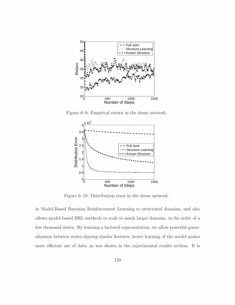
0 500 1000 150020

25

30

35

40

45

50

Number of Steps

Ret

urn

Full JointStructure LearningKnown Structure

Figure 6–9: Empirical return in the dense network.

0 500 1000 15000

0.5

1

1.5

2

2.5

3

3.5

4x 10

4

Number of Steps

Dis

trib

utio

n E

rror

Full JointStructure LearningKnown Structure

Figure 6–10: Distribution error in the dense network.

in Model-Based Bayesian Reinforcement Learning to structured domains, and also

allows model-based BRL methods to scale to much larger domains, in the order of a

few thousand states. By learning a factored representation, we allow powerful gener-

alization between states sharing similar features, hence learning of the model makes

more efficient use of data, as was shown in the experimental results section. It is

120

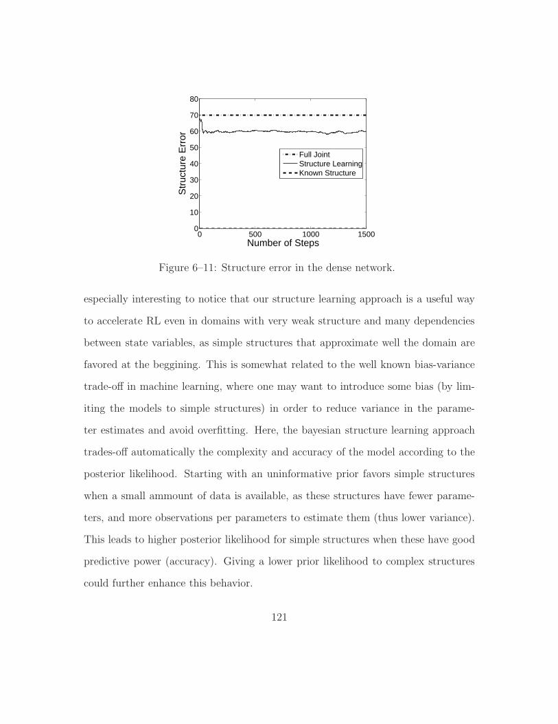
0 500 1000 15000

10

20

30

40

50

60

70

80

Number of Steps

Str

uctu

re E

rror

Full JointStructure LearningKnown Structure

Figure 6–11: Structure error in the dense network.

especially interesting to notice that our structure learning approach is a useful way

to accelerate RL even in domains with very weak structure and many dependencies

between state variables, as simple structures that approximate well the domain are

favored at the beggining. This is somewhat related to the well known bias-variance

trade-off in machine learning, where one may want to introduce some bias (by lim-

iting the models to simple structures) in order to reduce variance in the parame-

ter estimates and avoid overfitting. Here, the bayesian structure learning approach

trades-off automatically the complexity and accuracy of the model according to the

posterior likelihood. Starting with an uninformative prior favors simple structures

when a small ammount of data is available, as these structures have fewer parame-

ters, and more observations per parameters to estimate them (thus lower variance).

This leads to higher posterior likelihood for simple structures when these have good

predictive power (accuracy). Giving a lower prior likelihood to complex structures

could further enhance this behavior.

121

For future work, it would be interesting to extend this framework to partially

observable domains and continuous domains (i.e. Factored POMDP domains [34])

by combining the three frameworks that were presented in this thesis. For instance,

in the partially observable case, the Dirichlet count parameters φG would be only

partially observable through the observations z ∈ Z, as in the BAPOMDP case, so

that mixtures of Dirichlet would need to be used for the posterior over θG. These

mixtures could be maintained using particle filter algorithms similar to the ones

presented in Chapter 4. Furthermore, DBNs could also be used to represent the

observation function O, as in standard factored POMDP models. It would also be

interesting to improve the planning algorithm so that the structure can be exploited

to solve the planning problem more efficiently.

Another avenue of future research is to extend this approach to other types of

structured representations. For example, when using tile coding to represent the

dynamics of an MDP, one can view the tiling as a partition of the state space, which

can be represented as a tree. The current approach could be extended to learn

automatically the best tiling structure and the probability parameters for each tile

by doing MCMC over tree structures which partition the state space.

Finally, one last interesting idea would be to extend this framework for doing

automatic feature selection in RL. In domains described by many state features,

it might be desirable to approximate the system by only considering a subset of

the most important features, such as to reduce solving complexity and accelerate

learning. Selecting a subset of features would influence the likelihood of any DBN

restricted to this subset and therefore by doing MCMC over sets of features (in

122

addition to MCMC over DBN structures), one could find subsets of features which

approximate well the system.

123

CHAPTER 7

Conclusion

The problem of sequential decision-making under model uncertainty arises in

many practical applications of AI and decision systems. It is thus of critical im-

portance that such uncertainty be taken into account in planning algorithms for

robust decision-making. Furthermore, it is also important that such algorithms be

able to learn from past experience in order to improve their model (reduce model

uncertainty) and perform better in the future.

Model-based bayesian reinforcement learning methods address both problems

jointly by providing a framework that can simultaneously reduce the uncertainty on

the model, and plan optimal sequences of actions with respect to the current model

posterior (uncertainty), such as to maximize future expected return. However, the

applicability of these methods had been so far limited to simple and small domains.

This thesis focuses on presenting several extensions of model-based bayesian re-

inforcement learning methods and approximate algorithmic solutions that are appli-

cable in much more complex domains, such as to extend the applicability of model-

based bayesian reinforcement learning to problems encountered in the real world.

The first contribution is an extension of model-based BRL to partially observable

domains, such as to allow optimal decision-making under both state and model un-

certainty. Particle filter algorithms and an online planning algorithm were presented

124

to tractably find an approximate solution for this new framework. The second contri-

bution is an extension of model-based BRL to continuous (and partially observable)

domains. An appropriate choice of posterior distribution is identified and Monte

Carlo methods are proposed to tractably maintain the state and model uncertainty,

as well as find an approximate solution to the planning problem. Finally, the third

contribution is the presentation of a novel model-based BRL framework for MDPs

which can exploit underlying structure in the environment to learn more efficiently

in large domains.

Several ideas and suggestions for future work are discussed throughout this

thesis. In particular, the use of non-parametric bayesian methods in model-based

bayesian reinforcement learning seems a promising area of future research, such as

to provide a very general framework for sequential decision-making. While these

decision-making frameworks are attractive for their generality, representation power

and robustness to uncertainty, their computational solving complexity is currently

prohibitive for most practical applications. Developing more efficient approximate

inference and planning methods to handle these frameworks will ultimately be critical

to the successful application of these methods in practice.

As a next step, it would be important to validate these methods on real systems.

We believe that our current frameworks and algorithms could be applied on a real

robot to address several simple control tasks, such as moving to a particular goal

location or following another person, robot, or specific path. A more challenging

medical application we would like to address with such methods in the future is the

control of deep-brain electrical stimulation in the treatment of epilepsy [36].

125

Appendix A

Theorems and Proofs

This appendix presents the proofs of the theorems presented in Chapter 4 of

this thesis. Theorems 4.2.1 and 4.2.2 are presented first, then some useful lemmas

and the proofs of Theorems 4.3.1, 4.3.2 and 4.3.3.

Theorem 4.2.1. Let (S ′, A, Z, T ′, O′, R′, γ) be a BAPOMDP constructed from the

POMDP (S,A, Z, T, O,R, γ). If S is finite, then at any time t, the set S ′b′t

= {σ ∈

S ′|b′t(σ) > 0} has size |S ′b′t| ≤ |S|t+1.

Proof. Proof by induction. When t = 0, b′0(s, φ, ψ) > 0 only if φ = φ0 and ψ = ψ0.

Hence |S ′b′0| ≤ |S|. For the general case, assume that |S ′

b′t−1| ≤ |S|t. From the

definitions of the belief update function, b′t(s′, φ′, ψ′) > 0 iff ∃(s, φ, ψ) such that

b′t−1(s, φ, ψ) > 0, φ′ = φ + δass′ and ψ′ = ψ + δas′z. Hence, a particular (s, φ, ψ) such

that b′t−1(s, φ, ψ) > 0 yields non-zero probabilities to at most |S| different states in

b′t. Since |S ′b′t−1| ≤ |S|t by assumption, then if we generate |S| different probable state

in b′t for each probable state in S ′bt−1

, it follows that |S ′b′t| ≤ |S|t+1.

Theorem 4.2.2. For any horizon t, there exists a finite set Γt of functions S ′ → R,

such that V ∗t (b) = maxα∈Γt

∑

σ∈S′ α(σ)b(σ).

Proof. Clearly this is true for horizon t = 1, since V ∗1 (b) = maxa∈A

∑

(s,φ,ψ) b(s, φ, ψ)R(s, a).

Hence by defining Γ1 = {αa|αa(s, φ, ψ) = R(s, a), a ∈ A}, V ∗1 (b) = maxα∈Γ1

∑

σ∈S′ b(σ)α(σ).

Now assume that this is true for horizon t, we show that it must be true for hori-

zon t + 1. By assumption we have that there exist a set Γt such that V ∗t (b) =

126

maxα∈Γt

∑

σ∈S′ b(σ)α(σ).

Now V ∗t+1(b) = maxa∈A

[

∑

(s,φ,ψ) b(s, φ, ψ)R(s, a) +∑

z∈Z Pr(z|b, a)V ∗t (baz)

]

. Hence:

V ∗t+1(b) = maxa∈A

[

∑

(s,φ,ψ) b(s, φ, ψ)R(s, a) +∑

z∈Z Pr(z|b, a) maxα∈Γt

∑

σ∈S′ baz(σ)α(σ)]

= maxa∈A[

∑

(s,φ,ψ) b(s, φ, ψ)R(s, a) +∑

z∈Z maxα∈Γt

∑

σ∈S′ Pr(z|b, a)baz(σ)α(σ)]

= maxa∈A[

∑

(s,φ,ψ) b(s, φ, ψ)R(s, a)+

∑

z∈Z maxα∈Γt

∑

(s,φ,ψ)∈S′

∑

s′∈S b(s, φ, ψ)T sas′

φ Os′azψ α(s′,U(φ, s, a, s′),U(ψ, s′, a, z))

]

Thus if we define:

Γt+1 = {αa,f |αa,f(s, φ, ψ) = R(s, a)+∑

z∈Z∑

s′∈S Tsas′

φ Os′azψ f(z)(s′,U(φ, s, a, s′),U(ψ, s′, a, z)), a ∈ A, f ∈ [Z → Γt]},

then V ∗t+1(b) = maxα∈Γt+1

∑

σ∈S′ b(σ)α(σ) and Γt+1 is finite since |Γt+1| = |A||Γt||Z|,

which is finite by assumptions that A, Z and Γt are all finite.

For some of the following theorems, lemmas and proofs, we will sometime denote

the Dirichlet count update operator U , as defined for the BAPOMDP, as a vector

addition as follows: φ′ = φ+ δass′ = U(φ, s, a, s′), i.e. δass′ is a vector full of zeros, with

a 1 for the element φass′.

Lemma 7.0.1. For any t ≥ 2, any α-vector αt ∈ Γt can be expressed as αa,α′

t (s, φ, ψ) =

R(s, a) + γ∑

z∈Z∑

s∈S′ T sas′

φ Os′azψ α′(z)(s′, φ + δass′, ψ + δas′z) for some a ∈ A, and α′

a mapping Z → Γt−1.

Proof. Follows from proof of previous theorem (4.2.2).

Lemma 7.0.2. Given any a, b, c, d ∈ R, ab− cd = (a−c)(b+d)+(a+c)(b−d)2

127

Proof. Follows from direct computation.

Lemma 7.0.3. Given any φ, φ′ ∈ T , ψ, ψ′ ∈ O, then for all s ∈ S, a ∈ A, we have

that∑

s′∈S∑

z∈Z

∣

∣

∣

∣

φ′ass′ψ′as′z

N saφ′

N s′aψ′

−φass′ψas′z

N saφ N s′a

ψ

∣

∣

∣

∣

≤ DsaS (φ′, φ) + sups′∈SD

s′aZ (ψ′, ψ)

Proof. Using lemma 7.0.2, we have that:

∑

s′∈S∑

z∈Z

∣

∣

∣

∣

φ′ass′ψ′as′z

N saφ′

N s′aψ′

−φass′ψas′z

N saφ N s′a

ψ

∣

∣

∣

∣

= 12

∑

s′∈S∑

z∈Z

∣

∣

∣

∣

(

φ′ass′

N saφ′−

φass′

N saφ

) (

ψ′as′z

N s′aψ′

+ψas′z

N s′aψ

)

+

(

φ′ass′

N saφ′

+φass′

N saφ

) (

ψ′as′z

N s′aψ′

−ψas′z

N s′aψ

)∣

∣

∣

∣

≤ 12

∑

s′∈S

∣

∣

∣

∣

φ′ass′

N saφ′−

φass′

N saφ

∣

∣

∣

∣

∑

z∈Z

∣

∣

∣

∣

ψ′as′z

N s′aψ′

+ψas′z

N s′aψ

∣

∣

∣

∣

+ 12

∑

s′∈S

∣

∣

∣

∣

φ′ass′

N saφ′

+φass′

N saφ

∣

∣

∣

∣

∑

z∈Z

∣

∣

∣

∣

ψ′as′z

N s′aψ′

−ψas′z

N s′aψ

∣

∣

∣

∣

≤∑

s′∈S

∣

∣

∣

∣

φ′ass′

N saφ′−

φass′

N saφ

∣

∣

∣

∣

+ 12

[

sups′∈S∑

z∈Z

∣

∣

∣

∣

ψ′as′z

N s′aψ′

−ψas′z

N s′aψ

∣

∣

∣

∣

] [

∑

s′∈S

∣

∣

∣

∣

φ′ass′

N saφ′

+φass′

N saφ

∣

∣

∣

∣

]

=∑

s′∈S

∣

∣

∣

∣

φ′ass′

N saφ′−

φass′

N saφ

∣

∣

∣

∣

+ sups′∈S∑

z∈Z

∣

∣

∣

∣

ψ′as′z

N s′aψ′

−ψas′z

N s′aψ

∣

∣

∣

∣

= DsaS (φ′, φ) + sups′∈S D

s′aZ (ψ′, ψ)

Lemma 7.0.4. Given any φ, φ′,∆ ∈ T , then for all s ∈ S, a ∈ A, DsaS (φ+ ∆, φ′ +

∆) ≤ DsaS (φ, φ′) +

2N sa∆

∑

s′∈S |φass′

−φ′ass′

|(N sa

φ +N sa∆ )(N sa

φ′+N sa

∆ )

128

Proof. We have that:

DsaS (φ+ ∆, φ′ + ∆)

=∑

s′∈S

∣

∣

∣

∣

φass′

+∆ass′

N saφ +N sa

∆−

φ′ass′

+∆ass′

N saφ′

+N sa∆

∣

∣

∣

∣

=∑

s′∈S

∣

∣

∣

∣

(φass′

+∆ass′

)(N saφ′

+N sa∆ )−(φ′a

ss′+∆a

ss′)(N sa

φ +N sa∆ )

(N saφ +N sa

∆ )(N saφ′

+N sa∆ )

∣

∣

∣

∣

=∑

s′∈S

∣

∣

∣

∣

φass′

N saφ′

+φass′

N sa∆ +∆a

ss′N saφ′

−φ′ass′

N saφ −φ′a

ss′N sa

∆ −∆ass′

N saφ

(N saφ +N sa

∆ )(N saφ′

+N sa∆ )

∣

∣

∣

∣

≤∑

s′∈S

∣

∣

∣

∣

φass′

N saφ′

−φ′ass′

N saφ

(N saφ +N sa

∆ )(N saφ′

+N sa∆ )

∣

∣

∣

∣

+∑

s′∈S

∣

∣

∣

∣

N sa∆ (φa

ss′−φ′a

ss′)+∆a

ss′(N sa

φ′−N sa

φ )

(N saφ +N sa

∆ )(N saφ′

+N sa∆ )

∣

∣

∣

∣

≤∑

s′∈S

∣

∣

∣

∣

φass′

N saφ′

−φ′ass′

N saφ

N saφ N sa

φ′

∣

∣

∣

∣

+N sa

∆ [∑

s′∈S|φass′−φ′ass′ |]+

∣

∣

∣N saφ′

−N saφ

∣

∣

∣

∑

s′∈S ∆ass′

(N saφ +N sa

∆ )(N saφ′

+N sa∆ )

= DsaS (φ, φ′) +

N sa∆ [

∑

s′∈S|φass′−φ′ass′ |]+N sa

∆

∣

∣

∣N saφ′

−N saφ

∣

∣

∣

(N saφ +N sa

∆ )(N saφ′

+N sa∆ )

≤ DsaS (φ, φ′) +

2N sa∆

∑

s′∈S|φass′−φ′ass′|

(N saφ +N sa

∆ )(N saφ′

+N sa∆ )

Lemma 7.0.5. Given any ψ, ψ′,∆ ∈ O, then for all s ∈ S, a ∈ A, DsaZ (ψ + ∆, ψ′ +

∆) ≤ DsaZ (ψ, ψ′) +

2N sa∆

∑

z∈Z |ψasz−ψ′asz|

(N saψ +N sa

∆ )(N saψ′ +N sa

∆ ).

Proof. Same proof as for lemma 7.0.4, except that we sum over z ∈ Z in this case.

Lemma 7.0.6. Given any γ ∈ (0, 1), then supx γx/2x = 2

ln(γ−e)

Proof. We observe that when x = 0, γx/2x = 0 and limx→∞ γx/2x = 0. Furthermore,

γx/2 is monotonically decreasing exponentially as x increase while x is monotonically

increasing linearly as x increase. Thus it is clear that γx/2x will have a unique global

maximum in (0,∞). We will find it by taking the derivative:

129

∂∂x

(γx/2x)

= (ln γ)γx/2x2

+ γx/2

= γx/2( (ln γ)x2

+ 1)

Hence by solving when this is equal 0, we have:

γx/2( (ln γ)x2

+ 1) = 0

⇔ (ln γ)x2

+ 1 = 0

⇔ x = −2ln γ

= −2 logγ(e)

Hence we have that:

γx/2x

≤ −2γ− logγ(e) logγ(e)

= −2e−1 logγ(e)

= 2ln(γ−e)

Lemma 7.0.7. supα1∈Γ1,s∈S |α1(s, φ, ψ)− α1(s, φ′, ψ′)| = 0 for any φ, φ′, ψ, ψ′.

Proof. For any a ∈ A, s ∈ S, |αa1(s, φ, ψ)−αa1(s, φ′, ψ′)| = |R(s, a)−R(s, a)| = 0.

Theorem 4.3.1. Given any φ, φ′ ∈ T , ψ, ψ′ ∈ O and γ ∈ (0, 1), then for all t:

supαt∈Γt,s∈S

|αt(s, φ, ψ)− αt(s, φ′, ψ′)| ≤ 2γ||R||∞(1−γ)2 sup

s,s′∈S,a∈A

[

DsaS (φ, φ′) +Ds′a

Z (ψ, ψ′)+

4ln(γ−e)

(

∑

s′′∈S|φass′′−φ′ass′′ |

(N saφ +1)(N sa

φ′+1)

+∑

z∈Z|ψas′z−ψ′as′z|

(N s′aψ +1)(N s′a

ψ′ +1)

)]

130

Proof. Using lemma 7.0.1, we have that:

|αa,α′

t (s, φ, ψ)− αa,α′

t (s, φ′, ψ′)|

=

∣

∣

∣

∣

R(s, a) + γ∑

s′∈S∑

z∈Zφass′ψas′z

N saφ N s′a

ψ

α′(z)(s′, φ+ δass′, ψ + δas′z)

−R(s, a)− γ∑

s′∈S∑

z∈Zφ′ass′ψ′as′z

N saφ′

N s′aψ′

α′(z)(s′, φ′ + δass′, ψ′ + δas′z)

∣

∣

∣

∣

= γ

∣

∣

∣

∣

∑

s′∈S∑

z∈Z

[

φass′ψas′z

N saφ N s′a

ψ

α′(z)(s′, φ+ δass′, ψ + δas′z)−φ′ass′ψ′as′z

N saφ′

N s′aψ′

α′(z)(s′, φ′ + δass′, ψ′ + δas′z)

]∣

∣

∣

∣

= γ

∣

∣

∣

∣

∑

s′∈S∑

z∈Z

[

φass′ψas′z

N saφ N s′a

ψ

(α′(z)(s′, φ+ δass′, ψ + δas′z)− α′(z)(s′, φ′ + δass′, ψ

′ + δas′z))

−

(

φ′ass′ψ′as′z

N saφ′

N s′aψ′

−φass′ψas′z

N saφ N s′a

ψ

)

α′(z)(s′, φ′ + δass′, ψ′ + δas′z)

]∣

∣

∣

∣

≤ γ∑

s′∈S∑

z∈Zφass′ψas′z

N saφ N s′a

ψ

|α′(z)(s′, φ+ δass′, ψ + δas′z)− α′(z)(s′, φ′ + δass′, ψ

′ + δas′z)|

+γ∑

s′∈S∑

z∈Z

∣

∣

∣

∣

φ′ass′ψ′as′z

N saφ′

N s′aψ′

−φass′ψas′z

N saφ N s′a

ψ

∣

∣

∣

∣

|α′(z)(s′, φ′ + δass′, ψ′ + δas′z)|

≤ γ sups′∈S,z∈Z

|α′(z)(s′, φ+ δass′, ψ + δas′z)− α′(z)(s′, φ′ + δass′, ψ

′ + δas′z)|

+γ||R||∞1−γ

∑

s′∈S∑

z∈Z

∣

∣

∣

∣

φ′ass′ψ′as′z

N saφ′

N s′aψ′

−φass′ψas′z

N saφ N s′a

ψ

∣

∣

∣

∣

≤ γ sups′∈S,z∈Z

|α′(z)(s′, φ+ δass′, ψ + δas′z)− α′(z)(s′, φ′ + δass′, ψ

′ + δas′z)|

+γ||R||∞1−γ

(

DsaS (φ′, φ) + sups′∈SD

s′aZ (ψ′, ψ)

)

The last inequality follows from lemma 7.0.3. Hence by taking the sup we get:

supαt∈Γt,s∈S |αt(s, φ, ψ)− αt(s, φ′, ψ′)|

≤ γ sups,s′∈S,a∈A,z∈Z,αt−1∈Γt−1

|αt−1(s′, φ+ δass′, ψ + δas′z)− αt−1(s

′, φ′ + δass′, ψ′ + δas′z)|

+γ||R||∞1−γ sup

s,s′∈S,a∈A

(

DsaS (φ′, φ) +Ds′a

Z (ψ′, ψ))

131

We notice that this inequality defines a reccurence. By unfolding it up to t = 1 we

get that:

supαt∈Γt,s∈S |αt(s, φ, ψ)− αt(s, φ′, ψ′)|

≤ γt−1 supα1∈Γ1,s′∈S,∆∈T ,∆′∈O| ||∆||1=||∆′||1=(t−1)

|α1(s′, φ+ ∆, ψ + ∆′)− α1(s

′, φ′ + ∆, ψ′ + ∆′)|

+γ||R||∞1−γ

∑t−2i=1 γ

i sups,s′∈S,a∈A,∆∈T ,∆′∈O| ||∆||1=||∆′||1=i

(

DsaS (φ′ + ∆, φ+ ∆) +Ds′a

Z (ψ′ + ∆′, ψ + ∆′))

+γ||R||∞1−γ sup

s,s′∈S,a∈A

(

DsaS (φ′, φ) +Ds′a

Z (ψ′, ψ))

Applying lemmas 7.0.7, 7.0.4 and 7.0.5 to the last term, we get that:

supαt∈Γt,s∈S |αt(s, φ, ψ)− αt(s, φ′, ψ′)|

≤ γ||R||∞1−γ

∑t−2i=1 γ

i sups,s′∈S,a∈A,∆∈T ,∆′∈O| ||∆||1=||∆′||1=i

(

DsaS (φ′, φ) +Ds′a

Z (ψ′, ψ)

+2N sa

∆

∑

s′′∈S |φass′′

−φ′ass′′

|(N sa

φ +N sa∆ )(N sa

φ′+N sa

∆ )+

2N s′a∆′

∑

z∈Z |ψas′z

−ψ′as′z

|(N s′a

ψ +N s′a∆′ )(N s′a

ψ′ +N s′a∆′ )

)

+γ||R||∞1−γ sup

s,s′∈S,a∈A

(

DsaS (φ′, φ) +Ds′a

Z (ψ′, ψ))

= γ||R||∞1−γ

∑t−2i=1 γ

i/2 sups,s′∈S,a∈A,∆∈T ,∆′∈O| ||∆||1=||∆′||1=i

(

γi/2DsaS (φ′, φ) + γi/2Ds′a

Z (ψ′, ψ)

+2γi/2N sa

∆

∑

s′′∈S |φass′′

−φ′ass′′

|(N sa

φ +N sa∆ )(N sa

φ′+N sa

∆ )+

2γi/2N s′a∆′

∑

z∈Z |ψas′z

−ψ′as′z

|(N s′a

ψ +N s′a∆′ )(N s′a

ψ′ +N s′a∆′ )

)

+γ||R||∞1−γ sup

s,s′∈S,a∈A

(

DsaS (φ′, φ) +Ds′a

Z (ψ′, ψ))

132

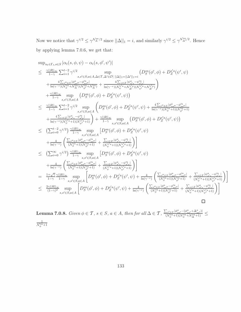
Now we notice that γi/2 ≤ γNsa∆ /2 since ||∆||1 = i, and similarly γi/2 ≤ γN

sa∆′/2. Hence

by applying lemma 7.0.6, we get that:

supαt∈Γt,s∈S |αt(s, φ, ψ)− αt(s, φ′, ψ′)|

≤ γ||R||∞1−γ

∑t−2i=1 γ

i/2 sups,s′∈S,a∈A,∆∈T ,∆′∈O| ||∆||1=||∆′||1=i

(

DsaS (φ′, φ) +Ds′a

Z (ψ′, ψ)

+4

∑

s′′∈S |φass′′

−φ′ass′′

|ln(γ−e)(N sa

φ +N sa∆ )(N sa

φ′+N sa

∆ )+

4∑

z∈Z |ψas′z

−ψ′as′z

|ln(γ−e)(N s′a

ψ +N s′a∆′ )(N s′a

ψ′ +N s′a∆′ )

)

+γ||R||∞1−γ sup

s,s′∈S,a∈A

(

DsaS (φ′, φ) +Ds′a

Z (ψ′, ψ))

≤ γ||R||∞1−γ

∑t−2i=1 γ

i/2 sups,s′∈S,a∈A

(

DsaS (φ′, φ) +Ds′a

Z (ψ′, ψ) +4

∑

s′′∈S |φass′′

−φ′ass′′

|ln(γ−e)(N sa

φ +1)(N saφ′

+1)

+4

∑

z∈Z |ψas′z

−ψ′as′z

|ln(γ−e)(N s′a

ψ +1)(N s′aψ′ +1)

)

+ γ||R||∞1−γ sup

s,s′∈S,a∈A

(

DsaS (φ′, φ) +Ds′a

Z (ψ′, ψ))

≤(∑t−2

i=0 γi/2

) γ||R||∞1−γ sup

s,s′∈S,a∈A

[

DsaS (φ′, φ) +Ds′a

Z (ψ′, ψ)

+ 4ln(γ−e)

(

∑

s′′∈S |φass′′

−φ′ass′′

|(N sa

φ +1)(N saφ′

+1)+

∑

z∈Z |ψas′z

−ψ′as′z

|(N s′a

ψ +1)(N s′aψ′ +1)

)]

≤(∑∞

i=0 γi/2

) γ||R||∞1−γ sup

s,s′∈S,a∈A

[

DsaS (φ′, φ) +Ds′a

Z (ψ′, ψ)

+ 4ln(γ−e)

(

∑

s′′∈S |φass′′

−φ′ass′′

|(N sa

φ +1)(N saφ′

+1)+

∑

z∈Z |ψas′z

−ψ′as′z

|(N s′a

ψ +1)(N s′aψ′ +1)

)]

=1+

√γ

1−γγ||R||∞

1−γ sups,s′∈S,a∈A

[

DsaS (φ′, φ) +Ds′a

Z (ψ′, ψ) + 4ln(γ−e)

(

∑

s′′∈S |φass′′

−φ′ass′′

|(N sa

φ +1)(N saφ′

+1)+

∑

z∈Z |ψas′z

−ψ′as′z

|(N s′a

ψ +1)(N s′aψ′ +1)

)]

≤ 2γ||R||∞(1−γ)2 sup

s,s′∈S,a∈A

[

DsaS (φ′, φ) +Ds′a

Z (ψ′, ψ) + 4ln(γ−e)

(

∑

s′′∈S |φass′′

−φ′ass′′

|(N sa

φ +1)(N saφ′

+1)+

∑

z∈Z |ψas′z

−ψ′as′z

|(N s′a

ψ +1)(N s′aψ′ +1)

)]

Lemma 7.0.8. Given φ ∈ T , s ∈ S, a ∈ A, then for all ∆ ∈ T ,∑

s′∈S |φass′

−(φass′

+∆ass′

)|(N sa

φ +1)(N saφ +N sa

∆ +1)≤

1N saφ +1

133

Proof.∑

s′∈S |φass′

−(φass′

+∆ass′

)|(N sa

φ +1)(N saφ +N sa

∆ +1)

=∑

s′∈S ∆ass′

(N saφ +1)(N sa

φ +N sa∆ +1)

= 1N saφ +1

(

N sa∆

N sa∆ +N sa

φ +1

)

The termN sa

∆

N sa∆ +N sa

φ +1is monotonically increasing and converge to 1 as N sa

∆ → ∞.

Thus the lemma follows.

Corollary 7.0.1. Given ε > 0, φ ∈ T , s ∈ S, a ∈ A, if N saφ > 1

ε− 1 then for all

∆ ∈ T we have that∑

s′∈S |φass′

−(φass′

+∆ass′

)|(N sa

φ +1)(N saφ +N sa

∆ +1)< ε

Proof. According to lemma 7.0.8, we know that for all ∆ ∈ T we have that∑

s′∈S |φass′

−(φass′

+∆ass′

)|(N sa

φ +1)(N saφ +N sa

∆ +1)≤

1N saφ +1

. Hence if N saφ > 1

ε− 1 then 1

N saφ +1

< ε.

Lemma 7.0.9. Given ψ ∈ O, s ∈ S, a ∈ A, then for all ∆ ∈ O,∑

z∈Z |ψasz−(ψasz+∆asz)|

(N saψ +1)(N sa

ψ +N sa∆ +1)

≤

1N saψ +1

Proof. Same proof as lemma 7.0.8.

Corollary 7.0.2. Given ε > 0, ψ ∈ O, s ∈ S, a ∈ A, if N saψ > 1

ε− 1 then for all

∆ ∈ O we have that∑

z∈Z |ψasz−(ψasz+∆asz)|

(N saψ +1)(N sa

ψ +N sa∆ +1)

< ε

Proof. Same proof as corollary 7.0.1 but using lemma 7.0.9 instead.

Theorem 4.3.2. Given any ε > 0 and (s, φ, ψ) ∈ S ′ such that ∃a ∈ A, s′ ∈ S,

N s′aφ > N ε

S or N s′aψ > N ε

Z , then ∃(s, φ′, ψ′) ∈ S ′ such that ∀a ∈ A, s′ ∈ S, N s′aφ′ ≤ N ε

S

and N s′aψ′ ≤ N ε

Z where |αt(s, φ, ψ)− αt(s, φ′, ψ′)| < ε holds for all t and αt ∈ Γt.

Proof. Consider an arbitrary ε > 0. We will first find a bound on N saφ and N sa

ψ such

that any vector with higher counts is within ε distance of another vector with lower

134

counts. Let’s define ε′ = ε(1−γ)28γ||R||∞ and ε′′ = ε(1−γ)2 ln(γ−e)

32γ||R||∞ . According to corollary 7.0.1,

we have that for any φ ∈ T such that N saφ > 1

ε′′− 1, then for all φ′ ∈ T such that

there exist a ∆ ∈ T where φ′ = φ + ∆, then∑

s′′∈S |φass′′

−φ′ass′′

|(N sa

φ +1)(N saφ′

+1)< ε′′. Hence we want

to find an N such that given φ ∈ T with N saφ > N , there exist a φ′ ∈ T such that

N saφ′ ≤ N , Dsa

S (φ, φ′) < ε′ and exists a ∆ ∈ T such that φ = φ′ + ∆. Let’s consider

an arbitrary φ such that N saφ > N . We can contruct a new vector φ′ as follows, for

all s′ define φ′ass′ =

⌊

Nφass′

N saφ′

⌋

and for all other a′ 6= a, s′′ 6= s define φ′a′s′′s′ = φa

′

s′′s′ for

all s′. Clearly φ′ ∈ T and such that N − |S| ≤ N saφ′ ≤ N . Moreover, we have that

φ′a′s′s′′ ≤ φa

′

s′s′′ for all s′, a′, s′′ and thus there will exist a ∆ ∈ T such that φ = φ′ + ∆.

Furthermore, from its construction we know that for all s′,

∣

∣

∣

∣

φ′ass′

N saφ′−

φass′

N saφ

∣

∣

∣

∣

≤ 1N saφ′

. Hence

it is clear from this that DsaS (φ, φ′) ≤ |S|

N−|S| . Thus, if we want DsaS (φ, φ′) < ε′, we

just need to take N > |S|(1+ε′)ε′

. Since we also want N > 1ε′′− 1, let’s just define

NS = max(

|S|(1+ε′)ε′

, 1ε′′− 1

)

. NS = N εS, as defined in Section 4.3, will be our bound

on N saφ such that, as we have just showed, for any φ ∈ T such that N sa

φ > NS, we can

find a φ′ ∈ T such that N saφ′ ≤ NS, D

saS (φ, φ′) < ε′ and

∑

s′′∈S |φass′′

−φ′ass′′

|(N sa

φ +1)(N saφ′

+1)< ε′′. Simi-

larly, since we have a similar corollary (corollary 7.0.1) for the observation counts ψ,

we can proceed in the same way and define NZ = max(

|Z|(1+ε′)ε′

, 1ε′′− 1

)

, such that

that for any ψ ∈ O such that N saψ > NZ , we can find a ψ′ ∈ O such that N sa

ψ′ ≤ NZ ,

DsaZ (ψ, ψ′) < ε′ and

∑

z∈Z |ψasz−ψ′asz |

(N saψ +1)(N sa

ψ′ +1)< ε′′. NZ = N ε

Z as we have defined in Section 4.3.

Now let S = {(s, φ, ψ) ∈ S ′|∀s′ ∈ S, a ∈ A,N s′aφ ≤ NS & N s′a

ψ ≤ NZ} and consider

an arbitrary (s, φ, ψ) ∈ S ′. For any s′ ∈ S, a ∈ A such that N s′aφ > NS, there exist a

φ′ ∈ T such that N s′aφ′ ≤ NS, D

s′aS (φ, φ′) < ε′ and

∑

s′′∈S |φas′s′′

−φ′as′s′′

|(N s′a

φ +1)(N s′aφ′

+1)< ε′′ (as we have

just showed above). Thus let’s define φas′s′′ = φ′as′s′′ for all s′′ ∈ S. For any s′ ∈ S,

135

a ∈ A such that N s′aφ ≤ NS, just set φas′s′′ = φas′s′′ for all s′′ ∈ S. Similarly, for any

s′ ∈ S, a ∈ A such that N s′aψ > NZ , there exist a ψ′ ∈ O such that N s′a

ψ′ ≤ NZ ,

Ds′aZ (ψ, ψ′) < ε′ and

∑

z∈Z |ψas′z

−ψ′as′z

|(N s′a

ψ +1)(N s′aψ′ +1)

< ε′′ (as we have just showed above). Thus let’s

define ψas′s′′ = ψ′as′s′′ for all s′′ ∈ S. For any s′ ∈ S, a ∈ A such that N s′a

ψ ≤ NZ ,

just set ψas′s′′ = ψas′s′′ for all s′′ ∈ S. Now it is clear from this construction that

(s, φ, ψ) ∈ S. By Theorem 4.3.1, for any t, supαt∈Γt,s∈S |αt(s, φ, ψ) − αt(s, φ, ψ)| ≤

2γ||R||∞(1−γ)2 sup

s,s′∈S,a∈A

[

Ds,aS (φ, φ) +Ds′,a

Z (ψ, ψ) + 4ln(γ−e)

(

∑

s′′∈S |φass′′

−φass′′

|(N sa

φ +1)(N saφ

+1)+

∑

z∈Z |ψas′z

−ψas′z

|(N s′a

ψ +1)(N s′aψ

+1)

)]

<

2γ||R||∞(1−γ)2

[

ε′ + ε′ + 4ln(γ−e)

(ε′′ + ε′′)]

= ε. This prooves the theorem.

Theorem 4.3.3. Given any ε > 0, (s, φ, ψ) ∈ S ′ and αt ∈ Γt computed from

the infinite BAPOMDP. Let αt be the α-vector representing the same condition-

nal plan as αt but computed with the finite BAPOMDP (Sε, A, Z, Tε, Oε, Rε, γ), then

|αt(Pε(s, φ, ψ))− αt(s, φ, ψ)| < ε1−γ .

Proof. Let (s, φ′, ψ′) = Pε(s, φ, ψ).

|αt(Pε(s, φ, ψ))− αt(s, φ, ψ)|

≤ |αt(s, φ′, ψ′)− αt(s, φ′, ψ′)|+ |αt(s, φ′, ψ′)− αt(s, φ, ψ)|

< |αt(s, φ′, ψ′)− αt(s, φ

′, ψ′)|+ ε (by Theorem 4.3.2)

= |γ∑

z∈Z∑

s′∈S Tsas′

φ′ Os′azψ′ [α′(z)(Pε(s′, φ′ + δass′, ψ

′ + δas′z))− α′(z)(s′, φ′ + δass′, ψ

′ + δas′z)] |+ ε

≤ γ∑

z∈Z∑

s′∈S Tsas′

φ′ Os′azψ′ |α′(z)(Pε(s′, φ′ + δass′, ψ

′ + δas′z))− α′(z)(s′, φ′ + δass′, ψ

′ + δas′z)|+ ε

≤ γ supz∈Z,s′∈S |α′(z)(Pε(s′, φ′ + δass′, ψ

′ + δas′z))− α′(z)(s′, φ′ + δass′, ψ

′ + δas′z)|+ ε

≤ γ supαt−1∈Γt−1,(s′,φ′′,ψ′′)∈S′ |αt−1(Pε(s′, φ′′, ψ′′))− αt−1(s

′, φ′′, ψ′′)|+ ε

136

Thus, we have that:

supαt∈Γt,σ∈S′ |αt(Pε(σ))− αt(σ)|

< γ supαt−1∈Γt−1,σ′∈S′ |αt−1(Pε(σ′))− αt−1(σ′)|+ ε

This defines a recurrence. By unfolding it up to t = 1, where ∀σ ∈ S ′, α1(Pε(σ)) =

α1(σ), we get that supαt∈Γt,σ∈S′ |αt(Pε(σ))− αt(σ)| < ε∑t−2

i=0 γi. Hence for all t, this

is lower than ε1−γ .

137

References

[1] K. J. Astrom. Optimal control of Markov decision processes with incompletestate estimation. Journal of Mathematical Analysis and Applications, 10:174–205, 1965.

[2] M. J. Beal, Z. Ghahramani, and C. E. Rasmussen. The infinite hidden Markovmodel. In Advances in Neural Information Processing Systems 14 (NIPS), pages577–584, 2002.

[3] R. Bellman. Dynamic Programming. Princeton University Press, 1957.

[4] B. Bonet. An epsilon-optimal grid-based algorithm for partially observableMarkov decision processes. In Proceedings of The Nineteenth International Con-ference on Machine Learning (ICML), pages 51–58, 2002.

[5] C. Boutilier, R. Dearden, and M. Goldszmidt. Stochastic dynamic programmingwith factored representations. Artificial Intelligence, 121(1-2):49–107, 2000.

[6] R. I. Brafman. A Heuristic variable grid solution method for POMDPs. InProceedings of the 14th National Conference on Artificial Intelligence (AAAI),pages 76–81, 1997.

[7] R. I. Brafman and M. Tennenholtz. R-max - a general polynomial time algorithmfor near-optimal reinforcement learning. Journal of Machine Learning Research,3:213–231, 2003.

[8] D. Braziunas and C. Boutilier. Stochastic local search for POMDP controllers.In The Nineteenth National Conference on Artificial Intelligence (AAAI), pages690–696, 2004.

[9] G. Casella and R. Berger. Statistical Inference. Duxbury Resource Center, 2001.

[10] A. Cassandra, M. L. Littman, and N. L. Zhang. Incremental pruning: a simple,fast, exact method for partially observable Markov decision processes. In Pro-ceedings of the Thirteenth Conference on Uncertainty in Artificial Intelligence(UAI), pages 54–61, 1997.

138

139

[11] P. S. Castro and D. Precup. Using linear programming for bayesian explorationin markov decision processes. In Proceedings of the 20th International JointConference on Artificial Intelligence (IJCAI), pages 2437–2442, 2007.

[12] H. Cheng. Algorithms for partially observable Markov decision processes. PhDthesis, University of British Columbia, 1988.

[13] R. Dearden, N. Friedman, and D. Andre. Model based bayesian exploration.In Proceedings of the 15th Conference on Uncertainty in Artificial Intelligence(UAI), pages 150–159, 1999.

[14] R. Dearden, N. Friedman, and S. J. Russell. Bayesian Q-learning. In AAAI,pages 761–768, 1998.

[15] M. H. DeGroot. Optimal Statistical Decisions. McGraw-Hill, 1970.

[16] J. L. Doob. Application of the theory of martingales. In Le Calcul des Prob-abilites et ses Applications. Colloques Internationaux du Centre National de laRecherche Scientifique, pages 23–27, 1949.

[17] A. Doucet, N. de Freitas, and N. Gordon. Sequential Monte Carlo Methods InPractice. Springer, 2001.

[18] R. O. Duda, P. E. Hart, and D. G. Stork. Pattern Classification (2nd Edition).Wiley-Interscience, 2000.

[19] M. Duff. Monte-Carlo algorithms for the improvement of finite-state stochas-tic controllers: Application to bayes-adaptive Markov decision processes. InProceedings of the 8th International Workshop on Artificial Intelligence andStatistics (AISTATS), 2001.

[20] M. Duff. Optimal Learning: Computational procedures for Bayes-adaptiveMarkov decision processes. PhD thesis, University of Massachusetts Amherst,Amherst, MA, 2002.

[21] D. Eaton and K. Murphy. Bayesian structure learning using dynamic program-ming and MCMC. In Proceedings of the 23rd Conference on Uncertainty inArtificial Intelligence (UAI), 2007.

[22] Y. Engel, S. Mannor, and R. Meir. Bayes meets Bellman: The gaussian processapproach to temporal difference learning. In Proceedings of the 20th Interna-tional Conference on Machine Learning (ICML), pages 154–161, 2003.

140

[23] Y. Engel, S. Mannor, and R. Meir. Reinforcement learning with gaussian pro-cesses. In Proceedings of the 22nd International Conference on Machine learning(ICML), pages 201–208, 2005.

[24] E. Even-Dar, S. M. Kakade, and Y. Mansour. Reinforcement learning in pomdpswithout resets. In Proceedings of the International Joint Conference on ArtificalIntelligence (IJCAI), pages 690–695, 2005.

[25] A. A. Feldbaum. Dual control theory, parts i and ii. Automation and RemoteControl, 21:874–880 and 1033–1039, 1961.

[26] N. M. Filatov and H. Unbehauen. Survey of adaptive dual control methods. InIEE Control Theory and Applications, volume 147, pages 118–128, 2000.

[27] D. A. Freedman. On the asymptotic behavior of bayes’ estimates in the discretecase. The Annals of Mathematical Statistics, 34:1386–1403, 1963.

[28] N. Friedman and D. Koller. Being Bayesian about Bayesian network structure:A Bayesian approach to structure discovery in Bayesian networks. MachineLearning, 50(1–2):95–125, 2003.

[29] M. Ghavamzadeh and Y. Engel. Bayesian actor-critic algorithms. In Proceedingsof the 24th international conference on Machine learning (ICML), pages 297–304, 2007.

[30] M. Ghavamzadeh and Y. Engel. Bayesian policy gradient algorithms. In Ad-vances in Neural Information Processing Systems 19 (NIPS), pages 457–464,2007.

[31] J. C. Gittins and D. Jones. Bandit processes and dynamic allocation indices.Journal of the Royal Statistical Society Series B, 41:148–177, 1979.

[32] G. J. Gordon. Approximate Solutions to Markov Decision Processes. PhD thesis,Carnegie Mellon University, 1999.

[33] A. Greenfield and A. Brockwell. Adaptive control of nonlinear stochastic systemsby particle filtering. In International Conference on Control and Automation(ICCA), pages 887–890, 2003.

[34] C. Guestrin, D. Koller, and R. Parr. Solving factored pomdps with linear valuefunctions. In IJCAI Workshop on Planning under Uncertainty and IncompleteInformation, 2001.

141

[35] C. Guestrin, D. Koller, R. Parr, and S. Venkataraman. Efficient solution algo-rithms for factored MDPs. Journal of Artificial Intelligence Research (JAIR),19:399–468, 2003.

[36] A. Guez, R. Vincent, M. Avoli, and J. Pineau. Adaptive treatment of epilepsyvia batch-mode reinforcement learning. In Proceedings of the 20th Innova-tive Applications of Artificial Intelligence Conference (IAAI), pages 1671–1678,2008.

[37] E. A. Hansen. An improved policy iteration algorithm for partially observableMDPs. In Tenth Neural Information Processing Systems 10 (NIPS), pages 1015–1021, 1998.

[38] M. Hauskrecht. Incremental methods for computing bounds in partially ob-servable Markov decision processes. In Proceedings of the Fourteenth NationalConference on Artificial Intelligence (AAAI), pages 734–739, 1997.

[39] D. Heckerman, D. Geiger, and D. M. Chickering. Learning bayesian net-works: The combination of knowledge and statistical data. Machine Learning,20(3):197–243, 1995.

[40] Edwin T. Jaynes. Prior probabilities. IEEE Transactions on Systems Scienceand Cybernetics, 4:227–241, 1968.

[41] H. Jeffreys. Theory of Probability. Oxford University Press, 1961.

[42] M. E. Johnson. Multivariate Statistical Simulation. John Wiley & Sons, Inc.,1987.

[43] L. P. Kaelbling. Learning in Embedded Systems. The MIT Press, 1993.

[44] L. P. Kaelbling, M. L. Littman, and A. R. Cassandra. Planning and actingin partially observable stochastic domains. Artificial Intelligence, 101:99–134,1998.

[45] R. E. Kass and L. Wasserman. The selection of prior distributions by formalrules. Journal of the American Statistical Association, 91:1343–1370, 1996.

[46] M. Kearns and S. Singh. Near-optimal reinforcement learning in polynomialtime. In Proceedings of the 15th International Conference on Machine Learning(ICML), pages 260–268, 1998.

142

[47] M. J. Kearns, Y. Mansour, and A. Y. Ng. A sparse sampling algorithm fornear-optimal planning in large markov decision processes. In Proceedings ofthe Sixteenth International Joint Conference on Artificial Intelligence (IJCAI),pages 1324–1331, 1999.

[48] M. L. Littman. Algorithms for sequential decision making. PhD thesis, BrownUniversity, 1996.

[49] M. L. Littman, T. L. Dean, and L. P. Kaelbling. On the complexity of solvingMarkov decision problems. In Proceedings of the 11th Annual Conference onUncertainty in Artificial Intelligence (UAI), pages 394–402, 1995.

[50] D. McAllester and S. Singh. Approximate Planning for Factored POMDPsusing Belief State Simplification. In Proceedings of the 15th Annual Conferenceon Uncertainty in Artificial Intelligence (UAI), pages 409–416, 1999.

[51] A. McCallum. Instance-based utile distinctions for reinforcement learning withhidden state. In International Conference on Machine Learning (ICML), pages387–395, 1995.

[52] N. Meuleau, L. Peshkin, K. Kim, and L. P. Kaelbling. Learning finite-statecontrollers for partially observable environments. In Proceedings of the FifteenthConference on Uncertainty in Artificial Intelligence (UAI), pages 427–436, 1999.

[53] G. E. Monahan. A survey of partially observable Markov decision processes:theory, models and algorithms. Management Science, 28(1):1–16, 1982.

[54] J. V. Neumann and O. Morgenstern. Theory of Games and Economic Behavior.Princeton University Press, 1944.

[55] S. Paquet, L. Tobin, and B. Chaib-draa. An online POMDP algorithm forcomplex multiagent environments. In Proceedings of The fourth InternationalJoint Conference on Autonomous Agents and Multi Agent Systems (AAMAS),pages 970–977, 2005.

[56] Judea Pearl. Probabilistic Reasoning in intelligent systems: Networks of plausi-ble inference. Morgan Kaufmann Publishers Inc., 1988.

[57] J. Pineau, G. Gordon, and S. Thrun. Point-based value iteration: an anytimealgorithm for POMDPs. In Proceedings of the Internation Joint Conference onArtificial Intelligence (IJCAI), pages 1025–1032, 2003.

143

[58] J. Pineau, G. Gordon, and S. Thrun. Anytime point-based approximations forlarge POMDPs. Journal of Artificial Intelligence Research, 27:335–380, 2006.

[59] P. Poupart and C. Boutilier. Bounded finite state controllers. In Advances inNeural Information Processing Systems 16 (NIPS), 2003.

[60] P. Poupart, N. Vlassis, J. Hoey, and K. Regan. An analytic solution to dis-crete bayesian reinforcement learning. In Proceedings of the 23rd internationalconference on Machine learning (ICML), pages 697–704, 2006.

[61] R. Ravikanth, S.P. Meyn, and L.J. Brown. Bayesian adaptive control of timevarying systems. In IEEE Conference on Decision and Control, pages 705–709,1992.

[62] S. Ross and B. Chaib-draa. Aems: An anytime online search algorithm forapproximate policy refinement in large POMDPs. In Proceedings of the 20thInternational Joint Conference on Artificial Intelligence (IJCAI), pages 2592–2598, 2007.

[63] S. Ross, B. Chaib-draa, and J. Pineau. Bayes-adaptive pomdps. In Advances inNeural Information Processing Systems 20, pages 1225–1232, 2008.

[64] Ilan Rusnak. Optimal adaptive control of uncertain stochastic discrete linearsystems. In IEEE International Conference on Systems, Man and Cybernetics,pages 4521–4526, 1995.

[65] S. J. Russell and P. Norvig. Artificial Intelligence: A Modern Approach (2ndEdition). Prentice Hall, 2002.

[66] J. K. Satia and R. E. Lave. Markovian decision processes with probabilisticobservation of states. Management Science, 20(1):1–13, 1973.

[67] L. Schwartz. On bayes procedures. Z. Wahrsch. Verw. Gebiete, 4:10–26, 1965.

[68] R. D. Smallwood and E. J. Sondik. The optimal control of partially observableMarkov processes over a finite horizon. Operations Research, 21(5):1071–1088,Sep/Oct 1973.

[69] T. Smith and R. Simmons. Heuristic search value iteration for POMDPs. In Pro-ceedings of the 20th Conference on Uncertainty in Artificial Intelligence (UAI),pages 520–527, 2004.

144

[70] T. Smith and R. Simmons. Point-based POMDP algorithms: improved analysisand implementation. In Proceedings of the 21th Conference on Uncertainty inArtificial Intelligence (UAI), pages 542–547, 2005.

[71] E. J. Sondik. The optimal control of partially observable Markov processes. PhDthesis, Stanford University, 1971.

[72] M. T. J. Spaan and N. Vlassis. Perseus: randomized point-based value iterationfor POMDPs. Journal of Artificial Intelligence Research, 24:195–220, 2005.

[73] A. L. Strehl and M. L. Littman. A theoretical analysis of model-based intervalestimation. In Proceedings of the 22nd International Conference on Machinelearning (ICML), pages 856–863, 2005.

[74] A.L. Strehl and M.L. Littman. An empirical evaluation of interval estimationfor Markov decision processes. In Proceedings of the 16th IEEE InternationalConference on Tools with Artificial Intelligence (ICTAI), pages 128–135, 2004.

[75] R. S. Sutton and A. G. Barto. Reinforcement Learning: An Introduction. TheMIT Press, 1998.

[76] S. Thrun, W. Burgard, and D. Fox. Probabilistic Robotics. The MIT Press,2005.

[77] T. Wang, D. Lizotte, M. Bowling, and D. Schuurmans. Bayesian sparse sam-pling for on-line reward optimization. In Proceedings of the 22nd internationalconference on Machine learning (ICML), pages 956–963, 2005.

[78] R. Washington. BI-POMDP: bounded, incremental partially observable Markovmodel planning. In Proceedings of the 4th European Conference on Planning,pages 440–451, 1997.

[79] C. J. C. H. Watkins and P. Dayan. Q-learning. Machine Learning, 8:279–292,1992.

[80] M. Wiering and J. Schmidhuber. Efficient model-based exploration. In Pro-ceedings of the fifth international conference on simulation of adaptive behavior,pages 223–228, 1998.

[81] R. Williams and L. Baird. Tight performance bounds on greedy policies basedon imperfect value functions. Technical Report NU-CCS-93-14, NortheasternUniversity, USA, 1993.

145

[82] Omar Zane. Discrete-time bayesian adaptive control problems with completeinformation. In IEEE Conference on Decision and Control, pages 2748–2749,1992.

[83] N. L. Zhang and W. Zhang. Speeding up the convergence of value iteration inpartially observable Markov decision processes. Journal of Artificial IntelligenceResearch, 14:29–51, 2001.

[84] R. Zhou and E. A. Hansen. An improved grid-based approximation algorithmfor POMDPs. In Proceedings of the Seventeenth International Joint Conferenceon Artificial Intelligence (IJCAI), pages 707–716, 2001.

KEY TO ABBREVIATIONS

AI: Artificial Intelligence

BACPOMDP: Bayes-Adaptive Continuous Partially Observable Markov Decision

Process

BAMDP: Bayes-Adaptive Markov Decision Process

BAPOMDP: Bayes-Adaptive Partially Observablt Markov Decision Process

BN: Bayesian Network

BRL: Bayesian Reinforcement Learning

DAG: Directed Acyclic Graph

DBN: Dynamic Beyesian Network

FSC: Finite State Controller

HSVI: Heuristic Search Value Iteration

LP: Linear Programming

MCMC: Markov Chain Monte Carlo

MDP: Markov Decision Process

PBVI: Point-Based Value Iteration

POMDP: Partially Observable Markov Decision Process

RL: Reinforcement Learning

146