Embed Size (px)
Citation preview
Model Based Automotive System Integration:
Fuel Cell Vehicle Hardware-In-The-Loop
by
Govind Goyal
A Thesis Presented in Partial Fulfillment
Of The Requirements for the Degree
Master of Science in Technology
Approved June 2014 by the
Graduate Supervisory Committee:
Abdel Ra’ouf Mayyas, Chair
Arunachalanadar Madakannan
Odesma Dalrymple
ARIZONA STATE UNIVERSITY
August 2014
i
ABSTRACT
Over the past decade, proton exchange membrane fuel cells have gained much
momentum due to their environmental advantages and commutability over internal
combustion engines. To carefully study the dynamic behavior of the fuel cells, a dynamic
test stand to validate their performance is necessary. Much attention has been given to
HiL (Hardware-in-loop) testing of the fuel cells, where the simulated FC model is
replaced by a real hardware. This thesis presents an economical approach for closed loop
HiL testing of PEM fuel cell. After evaluating the performance of the standalone fuel cell
system, a fuel cell hybrid electric vehicle model was developed by incorporating a battery
system. The FCHEV was tested with two different control strategies, viz. load following
and thermostatic.
The study was done to determine the dynamic behavior of the FC when exposed to
real-world drive cycles. Different parameters associated with the efficiency of the fuel
cell were monitored. An electronic DC load was used to draw current from the FC. The
DC load was controlled in real time with a NI PXIe-1071 controller chassis incorporated
with NI PXI-6722 and NI PXIe-6341 controllers. The closed loop feedback was obtained
with the temperatures from two surface mount thermocouples on the FC. The temperature
of these thermocouples follows the curve of the FC core temperature, which is measured
with a thermocouple located inside the fuel cell system. This indicates successful
implementation of the closed loop feedback. The results show that the FC was able to
satisfy the required power when continuous shifting load was present, but there was a
discrepancy between the power requirements at times of peak acceleration and also at

ii
constant loads when ran for a longer time. It has also been found that further research is
required to fully understand the transient behavior of the fuel cell temperature distribution
in relation to their use in automotive industry. In the experimental runs involving the
FCHEV model with different control strategies, it was noticed that the fuel cell response
to transient loads improved and the hydrogen consumption of the fuel cell drastically
decreased.

iii
ACKNOWLEDGMENTS
I would like to express my sincere thanks to professor Abdel Ra’ouf Mayyas for
his astounding support and help in this project. He helped me overcome the difficulties I
faced during the entire project. His willingness to help me every time I encountered an
issue helped me a lot to get through with this project. Without his guidance and profound
help, it would not have been possible for me to complete this project. In addition, I would
like to thank Professor Arunachalanadar Madakannan and Professor Odesma Dalrymple
who obliged me with being part of my committee. I would also like to express my
gratitude to Professor Arunachalanadar Madakannan for letting me use the fuel cell lab
and guiding me throughout the experiments.
Lastly, I would like to deeply thank my family, especially my wife for supporting
me accomplish this project. Without their blessings and love, I would not be able to
graduate in the stipulated time.
iv
TABLE OF CONTENTS
Page
LIST OF TABLES ...................................................................................................... vii
LIST OF FIGURES ................................................................................................... viii
NOMENCLATURE .................................................................................................... xi
CHAPTER
1: INTRODUCTION .................................................................................................... 1
Definitions: ............................................................................................................. 7
Acronyms: ............................................................................................................... 8
2: BACKGROUND ...................................................................................................... 9
Hardware-In-Loop Methodlogy: ........................................................................... 11
Scaling Of PEM Fuel Cells ................................................................................... 16
FCHEV: Energy Management Systems................................................................ 17
3: METHODOLOGY ................................................................................................. 23
Software Setup ...................................................................................................... 23
Vehicle Modelling ................................................................................................ 24
Driving Cycle ........................................................................................................ 25
Driver Block.......................................................................................................... 28
Powertrain Sub Model .......................................................................................... 29
Controller Block.................................................................................................... 30
Fuel Cell And Electric Motor System ................................................................... 31
Fuel Cell Subsystem ............................................................................................. 32
v
CHAPTER Page
Electric Motor Subsystem ..................................................................................... 34
Battery Subsystem ................................................................................................ 35
Control Strategy Implementation .......................................................................... 37
4: VEHICLE DYNAMICS ......................................................................................... 41
Rolling Resistance ................................................................................................ 42
Aerodynamic Drag ................................................................................................ 43
Grade Resistance ................................................................................................... 44
Model Description ................................................................................................ 45
5: HARDWARE SETUP ............................................................................................ 47
Hardware Components.......................................................................................... 48
HIL Methodology Implementation ....................................................................... 49
6: RESULTS AND DISCUSSION ............................................................................. 53
Power Consumption .............................................................................................. 67
Energy Consumption ............................................................................................ 70
H2 Consumption ................................................................................................... 71
Comparison With Honda FCX Clarity ................................................................. 73
Limitations Associated.......................................................................................... 75
7: CONCLUSIONS AND FUTURE SCOPE OF WORK ....................................... 777
REFERENCES ......................................................................................................... 799
APPENDIX
APPENDIX A ........................................................................................................... 844
ELECTRIC MOTOR SPECIFICATIONS ......................................................... 855
vi
APPENDIX Page
BATTERY SPECIFICATIONS ......................................................................... 855
APPENDIX B ........................................................................................................... 866
ENERGY CONSUMPTION RESULTS: FHDS & US06.................................. 867
APPENDIX C ........................................................................................................... 888
H2 CONSUMPTION RESULTS: FHDS &US06 .............................................. 889
vii
LIST OF TABLES
Table Page
1: Enthalpy and Entropy of fuel cell reaction according to temperature ...................... 3
2: Comparison of Energy Storage Systems .................................................................. 9
3: Fuel Cell Parameters [24, 30] ................................................................................. 32
4: Fuel Cell Constants ............................................................................................... 344
5: Vehicle Parameters [33] .......................................................................................... 44
6: H2 Consumption Comparison ................................................................................ 72
7: Fuel Economy Comparison: Honda FCX Clarity Vs Modelled Fuel Cell Vehicle
................................................................................................................................... 744

viii
LIST OF FIGURES
Figure Page
1: A fuel cell generating electricity from fuel (Barbir, Frano, 2013) ........................... 2
2: Block Diagram: FCHiL [3] ..................................................................................... 14
3: Hardware Setup: Dynamic Modeling and HiL Testing of PEMFC [22] ................ 15
4: Drive Structure of FC + B + UC hybrid vehicle [25] ........................................... 211
5: Rule Based Strategy [26] ...................................................................................... 222
6: Adaptive Load Strategy [26]................................................................................... 22
7: Top Level: Vehicle Modeling ................................................................................. 24
8: Federal Urban Driving Schedule Profile [28] ......................................................... 26
9: Federal Highway Driving Schedule Profile [28] .................................................... 26
10: Aggressive Urban Driving Schedule Profile [28] ................................................. 27
11: Acceleration Test Profile ...................................................................................... 27
12: Driver Subsystem Modeling ................................................................................. 28
13: Powertrain Subsystem Modeling .......................................................................... 30
14: Controller Subsystem Modeling Standalone FC ................................................ 311
15: Fuel Cell and Electric Motor Subsystem Modeling............................................ 322
16: Fuel Cell Subsystem Modeling ........................................................................... 333
17: Electric Motor Subsystem Modeling: FCHEV ..................................................... 35

ix
Figure Page
18: Battery Subsystem Modeling: FCHEV ................................................................ 35
19: Load Following Control Strategy: FCHEV .......................................................... 38
20: Thermostat Control Strategy: FCHEV ................................................................. 39
21: Forces Acting on a Vehicle [33] ........................................................................... 41
22: Vehicle Dynamics Subsystem Modeling .............................................................. 46
23: Basic hardware data flow for the closed-loop FCV HiL. ..................................... 47
24: HiL Hardware Setup ............................................................................................. 51
25: Thermocouple Placement ..................................................................................... 52
26: Tractive Force and EM Torque vs. Driving Cycle: FUDS ................................... 53
27: Tractive Force and EM Torque vs. Driving Cycle: FHDS ................................... 54
28: Tractive Force and EM Torque vs. Driving Cycle: US06 .................................... 55
29: Tractive Force and EM Torque vs. Driving Cycle: Acc Test ............................... 56
30: FC Standalone Desired and Base Power against Vehicle Speed: FUDS TEST ... 58
31: FC Standalone Desired and base power against Vehicle Speed: FHDS TEST .... 59
32: FC Standalone Desired and Base Power against Vehicle Speed: US06 TEST .... 60
33: FC Standalone Desired & Base Power against Vehicle Speed: Acc Test ............ 61
34: Fuel Cell Stack Temperature: FC Standalone: FUDS .......................................... 62
35: Fuel Cell Stack Temperature: FC Standalone: FHDS .......................................... 63

x
Figure Page
36: Fuel Cell Stack Temperature: FC Standalone: US06 ........................................... 64
37: Fuel Cell Stack Temperature: FC Standalone: Acceleration test ......................... 65
38: FC Power Comparison – FC Standalone vs FCHEV: FUDS ............................... 67
39: FC Power Comparison – FC Standalone vs FCHEV: FHDS ............................... 68
40: FC Power Comparison – FC Standalone vs FCHEV: US06 ................................ 69
41: Energy Comparison – FC Standalone vs FCHEV: FUDS .................................... 70
42: H2 Consumption Comparison – FC Standalone vs FCHEV: FUDS .................... 71
43: Energy Comparison– FC Standalone vs FCHEV: FHDS ................................... 877
44: Energy Comparison– FC Standalone vs FCHEV: US06 .................................... 877
45: H2 Consumption Comparison – FC Standalone vs FCHEV: FHDS .................. 899
46: H2 Consumption Comparison – FC Standalone vs FCHEV: US06 ................... 899

xi
NOMENCLATURE
m- Vehicle mass
g- Gravitational acceleration
fr- Rolling resistance
Cd- Drag coefficient
Af- Frontal area
Ƿ- Air density
𝛿- Rotational mass coefficient
Pfc- Output power of the fuel cell
Alpha – Accelerator pedal position
Beta - Brake pedal position
T_em_req – Torque requested from the electric motor
FC_V – Fuel cell voltage
M_H2 – Fuel cell hydrogen consumption
P_net – Net power produced by the fuel cell
N_FC – Number of stack cells
Lhv_FC – Lower heating value of fuel in fuel cell

1
1: INTRODUCTION
The current automotive scenario has seen a rapid growth in the use of hybrid energy
systems. With the increasing applications of these systems, comes the necessity to
efficiently test and develop cost effective and energy efficient systems. The testing of
hybrid systems involves many factors and real hardware testing would increase the costs
[1]. On the other hand, testing, based exclusively on simulation of the system would lack
compatibility with the real world. Thus, a promising approach to deal with this issue is
the Hardware-in-the-loop (HiL) methodology, which has been proved more practical and
useful [1, 2, and 3]. This project uses HiL methodology to test a real Polymer Electrolyte
Membrane (PEM) hydrogen fuel cell in a closed loop system. The aim of this project is to
present a model-based test system where the simulated fuel cell is replaced with the real
hardware component, and obtain a fast dynamic response between the simulated model
and real hardware in a closed loop.
A Fuel Cell (FC) is an electrochemical device capable of producing electricity from
chemical reactions [4]. It is different from a battery in a way that energy is not stored, but
produced as and when required. Although many research and experiments are going on
for reducing the cost and fuel consumption of fuel cells, the basic principle behind the
working of the fuel cells remains the same [5]. The conventional way of harnessing
mechanical energy from internal combustion engines involves the following steps [6]:
1. Fuel is injected into the cylinders according to the fuel-air ratio.
2. Fuel combustion converts chemical energy of the fuel into heat energy.
2
3. The heat energy is used to move the piston in the cylinders.
4. The conversion of heat energy into mechanical energy helps rotating the shaft
coupled to the wheels.
On the other hand, in fuel cells, the fuel generates electricity in just one step,
eliminating the 4 step process (Figure 1) [7]. This ease of producing electricity has
attracted many applications of fuel cells over the past few years.
Figure 1: A fuel cell generating electricity from fuel (Barbir, Frano, 2013)
A typical PEM fuel cell consists of two electrodes, anode and the cathode. The
electrochemical reactions occur simultaneously on both the electrodes, and are given as
[4]:
H2 → 2H+ + 2e , at the anode (1)
1
2𝑂2 + 2𝐻+ + 2𝑒 → 𝐻2𝑂 , at the cathode (2)
3
In the overall reaction, heat is produced along with water and electricity. The heat
of formation of water in liquid form is -286 kJ/mol [4]. Therefore, the overall reaction
can be written as:
𝐻2 +
1
2𝑂2 → 𝐻2𝑂 − 286 𝑘𝐽𝑚𝑜𝑙−1
(3)
Temperature plays an important role in the efficiency of the fuel cell. The cell
potential of the fuel cell changes with change in temperature. The enthalpy and entropy
of the overall reaction are a function of temperature. The specific heat of gas is also a
function of the temperature. The following table shows the changes in the enthalpy and
entropy the overall fuel cell reaction according to the temperature [8].
T(K) ∆H (kJ/mol) ∆S (kJ/mol)
298.15 -286.02 -0.16328
333.15 -284.85 -0.15975
353.15 -284.18 -0.15791
373.15 -283.52 -0.15617
Table 1: Enthalpy and Entropy of fuel cell reaction according to temperature
Thus as seen from the table, temperature of the fuel cell stack plays a vital role as far
as the efficiency is concerned. For this purpose, the water produced in the fuel cell
reaction is used to cool the stack. This is one of the many ways in operation to cool the
fuel cell. Depending on the applications, fuel cells can be air-cooled or water-cooled.
The preferred type of Fuel Cell for automotive applications is the PEM (Proton
Exchange Membrane) FC, which has advantages of faster start-ups and low operating
temperature, ideal for automotive use [9].

4
The fuels used are hydrogen and oxygen, and their availability in pure form can be
an issue [4]. However, FC systems can be a great source of energy in the long run for
automotive as well as for stationary systems applications.
The core of a PEM fuel cell is the polymer or the proton exchange membrane [4]. The
electrodes are present on either side of the membrane. The electrodes must be porous in
order to diffuse the gases into the membrane. The electrochemical reactions take place on
the catalyst present on the electrodes or the membrane. This assembly of the electrodes
and the membrane is often referred to as the membrane electrode assembly (MEA) [4].
The generic materials used in the PEM fuel cell for the purpose of the membrane are
made of perfluorocarbon sulphonic acid (PSA). The process of energy conversion in a
PEM fuel cell takes place in the following steps [4]:
1. Gases flow from the supply channels to the porous electrodes.
2. Electrochemical reactions at the anode and the cathode.
3. Transport of protons through the proton exchange membrane.
4. Induced electric current through conductive cell components.
5. Transport and utilization of water or water vapor from the membrane.
Thus, the construction and designing of a PEM fuel cell must be able to efficiently
accommodate these processes. The fuel cell membrane must manifest high conductivity
for the exchange of protons, must exhibit a sufficient barricade for the reactions of gases,
and be chemically as well as mechanically stable.

5
Fuel Cell Vehicles (FCV) have proved to be more advantageous than traditional
conventional vehicles using internal combustion engines, as they are a clean source of
energy with no combustion as compared to IC engines. Furthermore, FCV have higher
efficiency against IC engines [10]. However, these advantages cannot alone lead to
replacement of IC engines. FCV have to cope with other factors such as cost
effectiveness, fuel availability, etc. Such modifications or rather developments require a
test procedure capable of efficiently testing and recording the determining factors. One
such approach is a closed loop HiL approach.
This project aims at developing one such closed-loop HiL test bench based on a
mathematical model of a fuel cell hybrid vehicle. The project is performed with a goal to
quantify the performance characteristics of a fuel cell driven vehicle. The HiL test bench
is used to validate the standalone fuel cell vehicle model. The results were compared to
the fuel cell data procured from the fuel cell under experiment.
The project continues with the development of a hybrid electric simulation model of
the fuel cell vehicle. The hybridization of the fuel cell was achieved by incorporating a
battery and an electric model into the standalone fuel cell. Furthermore, different energy
management strategies (EMS) were compared to make conclusion on the efficiency of
the fuel cell hybrid electric vehicle under different control strategies. The fuel cell hybrid
vehicle was run under the load following and thermostatic control strategies. Load
following control strategy is based on the load demands by the driving cycle, whilst the
thermostatic control strategy pays attention towards maintaining the battery SOC. These
strategies allow the fuel cell to be tested in two different driving scenarios.

6
The further report is organized as follows:
Chapter 2 summarizes a literature review pertaining to fuel cell vehicle modelling
and testing, development and implementation of control strategies.
Chapter 3 presents the methodology of the project in a detailed format. It covers
topics of software setup, hardware setup and HiL methodology. Procedures and
concepts used in vehicle modelling and testing are explained in this section
Chapter 4 presents the results and discussions based on the experimental data.
Chapter 5 presents the conclusions, recommendations and future scope of the
project based on the results.

7
Definitions:
Hardware-in-the-loop (HiL): A technique used in test and development complex real-
time systems, where the product under test is replaced with the real hardware in
simulation.
Vehicle Simulation: A technique involving virtually designing an automotive system,
such as passenger cars with the aide of simulation software, which can be run in the
software environment for research purposes.
Regenerative braking: A mechanism, which slows down a vehicle by converting the
kinetic energy at the wheels into electric energy, which would be usually lost in
conventional braking.
Drive cycle: A set of pre-defined data points indicating the desired velocity of the
vehicle against the time.
Tractive force: The part of the tractive effort generated by a vehicle’s power source,
which aids in the forward motion of the vehicle.
Mass flow rate: The mass of a substance flowing over a given point or surface per
unit time.
8
Acronyms:
FCV: Fuel Cell Vehicle
BEV: Battery Electric Vehicle
FCHEV: Fuel Cell Hybrid Electric Vehicle
EPA: Environmental Protection Agency
FUDS: Federal Urban Driving Schedule
FHDS: Federal Highway Driving Schedule
PID: Proportional-Integral-Derivative Controller
PEM: Proton/Polymer Exchange/Electrolyte Membrane
NI: National Instruments
PXI: PCI eXtensions for Instrumentation
SOC: State of Charge

9
2: BACKGROUND
Automotive industry has seen a recent shift of focus from internal combustion engine
drivetrains to alternative fueled drivetrains. Battery operated vehicles are a good choice
where low noise and pollution are required. Battery Electric Vehicles (BEV’s) come with
disadvantages in storage system capacities, charging times, operating temperature range
and many more. However immense growth has been recorded in the developed battery
systems for automotive applications in the recent years [13], [14].
Hydrogen fuel cells have attracted attention of researchers over the past few years due
to some of the advantages they have to offer over batteries. One of them being
recharging, which can be achieved in around 5 minutes as compared to the batteries
required for a 100 kW powertrain system, typical for a passenger propulsion vehicle [10].
Proton Exchange Membrane fuel cells have been the center of attraction due to the
advantages they offer, some of them being compactness, lightweight and operating range.
The following table shows the comparison of various energy storage systems [13],
[14].
Hydrogen (70 MPA
Pressure Vessel
Li-ion Battery Ni-MH Battery
Specific Energy 1600 Wh/kg 120 Wh/kg 70 Wh/kg
Energy Density 770 Wh/l 50 Wh/l 140 Wh/l
Energy required for
vehicle range 500 kM
200 kWh 100 kWh 100 kWh
Cost (at volume
production)
USD 3600 USD 40000 USD 30000
Table 2: Comparison of Energy Storage Systems
10
The use of hydrogen fuel cells in the propulsion of vehicles eliminates the issue of
emissions, which has been a topic of debate in the automotive industry since decades
[15]. Their use also would provide higher overall efficiencies as compared to
conventional or BEV’s. General Motors introduced the first FCV in 1966 named the
Electrovan, which used alkaline electrolyte, liquid oxygen and hydrogen, which were
stored in cryogenic vessels [16].
The major issue regarding FCV that has been encountered is the production and
storage of hydrogen. Hydrogen can be produced by various methods [17]. Currently the
most commonly used method is the steam reforming method from hydrocarbons. Steam
reforming is a direct method of production of hydrogen from natural gas or other
hydrocarbons with an efficiency of around 80% [17]. Other methods of hydrogen
production could be electrolysis and thermolysis.
Storage of hydrogen can be achieved using following three major options [17]:
CGH2- Compressed gaseous hydrogen - 35–70MPa (room temperature).
Solid-state absorbers (such as hydrides or high-surface materials).
LH2 - Liquid hydrogen - 20–30 K, 0.5–1 MPa.
11
GM HydroGen3 was a prototype car manufactured by Opel (a subsidiary of GM)
which was under test in Japan [18]. HydroGen4 has succeeded it in 2007 [18]. The fuel
cell system of the car fits in the same volume as the conventional system of same power.
This provides with an advantage of replacing the energy storage system of existing
vehicles without going through major design modifications. Major automotive
manufacturers around the globe have introduced FCV’s over the past decade and even
before, and the race continues.
Although, fuel cells pose very attractive for automotive applications, they have to
cope up with disadvantages they inherit when compared to the current automotive
scenario. These can be vehicle range, fuel storage and cost to name a few. Extensive
research is going on and more is needed to be done to make fuel cells capable of
overcoming the nonrenewable automotive fuel options. This requires an efficient test set
up that can be dynamically altered without making major changes and is cost effective
[19].
Hardware-In-Loop Methodlogy:
HiL methodology has been proved to be much helpful in the testing and validation of
hardware components in the automotive industry. One of the major applications of this
methodology has been the testing and validation of control algorithms for powertrains
and analyzing the behavior of hardware components by simulating the vehicle
environment, which would otherwise require many hardware components to be tested in
real world [20].

12
This would not only increase cost by manifolds but also would require higher level of
expertise. Fuel cell hardware-in-the-loop is a relatively newer concept. The methodology
revolves around the concept of having a vehicle simulation model and replacing the
hardware component to be tested with the real hardware. There are many ways to test the
hardware component in HiL. One of the ways, which is proven more efficient than the
attempts made over the past few years, has been proposed in this project.
A few years back, PLC (Programmable Logic Controllers) were in use for
commissioning the HiL methodology [20]. PLC is a computer control system used for
monitoring the inputs based on the custom program to give to control the outputs. It’s a
digital computer currently used in the fields of process control and automation. This
required use of Ethernet communication between the host PC and the PLC. This in turn
increased the complexity of the HiL. With the increased number of components
associated with PLC’s, it became difficult to find errors and make connections.
Moreover, setting up the communication between the host PC, PLC and the hardware to
be tested posed some challenges.
The Hawaii Naturals Energy Institute (HNEI) of the University of Hawaii has been
one of the first few to apply and demonstrate the HiL on fuel cells [3]. They have
developed a dynamic fuel cell test system demonstrating a unique test bench for the
design evaluation of fuel cells with applications in automotive industry. The first HiL
implementation at the HNEI facility was commissioned in January –February 2006. They
have been using HiL to evaluate the dynamic behavior of fuel cells in automotive
applications.
13
There have been many successful attempts recently to test the fuel cell system in HiL
[21, 22, and 23]. In a preliminary attempt by R.M. Moorea et al. in his research work
titled ‘Fuel Cell Hardware-in-Loop’ [3], he and other authors have proposed the Hil
methodology for fuel cell system design and evaluation. The work describes the use of a
dynamic simulation tool, FCVSim for the simulation of the fuel cell vehicle.
The simulated model consists of the driver block representing the driver properties
and characteristics. The driver block gives a command for the acceleration or brake based
on the desired and current vehicle velocity. It acts as the controller for the vehicle
simulation model.
The vehicle controls block monitors the accelerator and brake pedal position. Based
on the acceleration or the brake commands received, the block demands torque to be
given at the wheels in case of acceleration, or applies regenerative braking or
conventional braking on the wheels in case of braking.
The powertrain block consists of the various power components of the vehicle. In this
case, the authors have used an electric motor for power transmission between the fuel cell
system and the wheels. This required the use of a transmission, which was modelled in
the same block.
The input to the driver block were to be the standard driving cycles. The power
demanded by the drive train was obtained from the fuel cell. Fuel cell gave the voltage
output, which was given as a feedback to the drive train block.
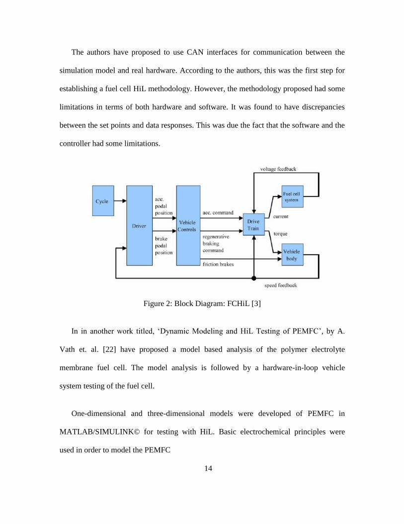
14
The authors have proposed to use CAN interfaces for communication between the
simulation model and real hardware. According to the authors, this was the first step for
establishing a fuel cell HiL methodology. However, the methodology proposed had some
limitations in terms of both hardware and software. It was found to have discrepancies
between the set points and data responses. This was due the fact that the software and the
controller had some limitations.
Figure 2: Block Diagram: FCHiL [3]
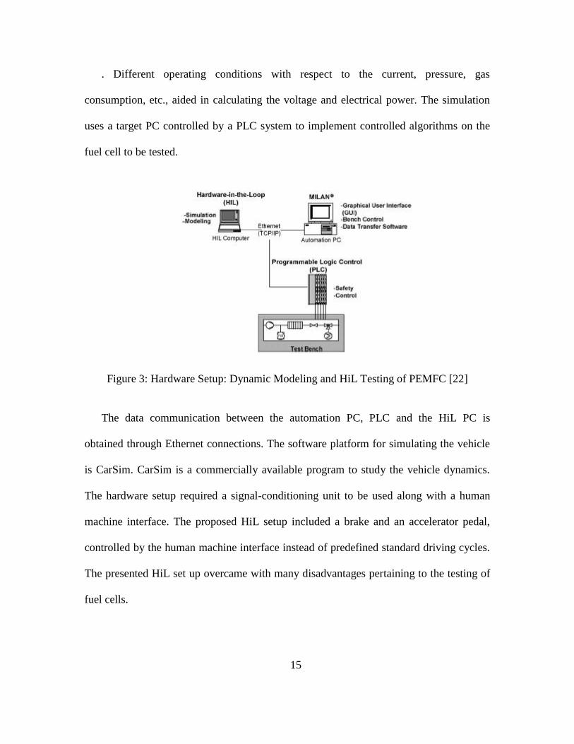
In in another work titled, ‘Dynamic Modeling and HiL Testing of PEMFC’, by A.
Vath et. al. [22] have proposed a model based analysis of the polymer electrolyte
membrane fuel cell. The model analysis is followed by a hardware-in-loop vehicle
system testing of the fuel cell.
One-dimensional and three-dimensional models were developed of PEMFC in
MATLAB/SIMULINK© for testing with HiL. Basic electrochemical principles were
used in order to model the PEMFC
15
. Different operating conditions with respect to the current, pressure, gas
consumption, etc., aided in calculating the voltage and electrical power. The simulation
uses a target PC controlled by a PLC system to implement controlled algorithms on the
fuel cell to be tested.
Figure 3: Hardware Setup: Dynamic Modeling and HiL Testing of PEMFC [22]
The data communication between the automation PC, PLC and the HiL PC is
obtained through Ethernet connections. The software platform for simulating the vehicle
is CarSim. CarSim is a commercially available program to study the vehicle dynamics.
The hardware setup required a signal-conditioning unit to be used along with a human
machine interface. The proposed HiL setup included a brake and an accelerator pedal,
controlled by the human machine interface instead of predefined standard driving cycles.
The presented HiL set up overcame with many disadvantages pertaining to the testing of
fuel cells.
16
Scaling Of PEM Fuel Cells
Automotive applications require fuel cells to be capable of producing at least 80-
100kW rated power. Testing s fuel cell system with such a power would not only be
complex, but also very costly, keeping in mind the current cost scenario of fuel cells.
Procuring such a huge fuel cell system would require fuel to that extent. That is a major
issue, due to the problems of obtaining hydrogen fuel.
Many experiments have been done over the past years to test the scalability of PEM
fuel cells [23]. It has been found that PEM fuel cells are scalable in terms of power,
voltage and current. Since then, researchers have extensively done per unit analysis of
fuel cells [23]. Per-unit analysis refers to using scaled values of parameters under test.
Using such kind of testing makes the test bench independent of power rating of the
application. It also adds up to the flexibility of the applications.
As in case of HiL, the component to be tested is replaced as real hardware in the
simulation model. The scalability of the PEM fuel cells renders perfect as the system
components related to the hybrid vehicle, such as battery, electric motor, etc. can be
scaled according to the fuel cell and the application under test and still be able to provide
the required results with almost no increase in costs.
However, the closed-loop HiL possesses an advantage over an open loop HiL, as
there is a feedback from the system under test. By using a feedback, the system can be
controlled in real-time, and some of the critical parameters can be measured to limit the
operation or take appropriate steps. Since they are inherently sensitive to temperature, in
17
this study, the temperature of the fuel cell stack has been considered as the critical
parameter in relation to the performance of the fuel cell. The temperature of the fuel cell
is of paramount importance. The fuel cell used in the testing is a PEM fuel cell.
Electricity is produced by the conductivity of the membrane and this conductivity is
directly proportional to the water content present [7]. In the PEM FC, the hydrogen from
anode reacts with the oxygen at cathode to produce water along with heat and electricity.
The heat produced in this reaction is greater than the water produced [4], leading to an
increase in the temperature of the system. Higher temperature may lead to dryness of the
membrane and thus decrease the efficiency of the fuel cell. Further, it may damage the
system [4]. Hence, to keep the FC efficiently running, the temperature of the FC stack
system has to be monitored and controlled. Research is been going on to devise ways for
heat dissipation from a FC system [21].
FCHEV: Energy Management Systems
Hybridization of standalone internal combustion engines has opened many ways to
increase the efficiency of IC engines. IC engines cannot give a maximum efficiency at all
loads during variable driving conditions. With the tool of hybridization, the IC engines
can be operated at loads to give maximum efficiency, thus resulting in higher fuel
economy. The energy efficiency of IC engines at low loads is lower, as compared to the
rated loads. The battery and electric motor system provide power for these low loads.
18
On the other hand, FCV’s do not giver lower efficiency on part loads. In fact, the
efficiency is higher at low loads. This presents as a major advantage of FCHEV’s in
comparison to IC engine vehicles. In many of the studies conducted, it has been found
that the efficiency of FCHEV’s can be 2.5-3 times the efficiencies of ICE vehicles [17]
Although the fuel cells are more efficient at part loads, hybridization can be
advantageous in many ways. One of them being to recover the braking energy called as
regenerative braking, which would conventionally be lost as heat. This energy is stored in
battery and can be reused. Another objective being to assist the fuel cell at higher loads,
when the fuel cell is not able to meet the power requirements. This in turn reduces the
hydrogen consumption of the fuel cell, thus reducing the cost.
With the need of hybridization, arises the need of developing a control strategy for
managing the energy distribution between the fuel cell and the battery. Over the past few
years, many studies and research have been conducted to find the optimal control strategy
for energy management system of FCHEV’s. In a study conducted by R. K. Ahluwalia et
al. [24], the author have proposed an energy management system to operate the fuel cell
system in load following mode and the energy storage system in charge sustaining mode.
The main objective in the research presented was to maintain the charge of the energy
storage system in a predefined range and to assist the fuel cell at peak loads, when the
fuel cell was not able to meet the power demands. In the load following control strategy,
the power distribution is based on the load or power demands.
19
The fuel cell system provides power for normal driving conditions, whereas the
energy storage system (ESS) provides transient and peak powers. The ESS also stores the
energy harnessed from regenerative braking.
Simulation analysis of fuel cell and ESS combined in the urban and city drive cycles
have been conducted in order to size the power train components. Computer codes such
as GCtool and PSAT have been employed for the analysis. According to the simulation
tests conducted, promising results in the hybridization as compared to conventional ICE
engines have been seen. The results show an efficiency increase of as high as 27% in the
city drive cycle. This increase in fuel economy is a result of the stop and go’s present in
the city drive cycle. On the highway drive cycle, the increase in efficiency was notices to
be 15%.
In a paper presented by Qi Li et al. [25], the authors have proposed an energy
management system based on fuzzy logic. The research presents the comparison between
the efficiencies of the fuel cell and battery hybrid system, compared to fuel cell, battery
and ultracapacitor hybrid system. In the fuel cell and battery system, the battery is
connected across the fuel cell to provide power for start-ups. In the battery plus
ultacapacitor system, the power required at start-ups, acceleration and peak loads, is
provided by the duo.
The fuzzy logic control works on a set of “if then rules”. The ‘If’ part checks for a
condition or a set of conditions, and the ‘then’ part represents the set of outcomes.
20
According to the importance of parameters, the authors have chosen the ‘If’ conditions to
be satisfied and the results are calculated based on the average of the conditions satisfied.
The power demand of the electric motor and the battery SOC (State of charge) have
been chosen to be the input variables and the power demand from the fuel cell is
determined by these two conditions. The authors have developed four driving modes for
the fuzzy logic control:
1. Starting Mode: Here the start-up power is provided by the battery independently. The
fuel cell power is actuated as the demand power increases over time.
2. Fuel cell driving mode: In this mode, the power is solely provided by the fuel cell and
the battery is charged. This mode is actuated if the SOC of the battery drops below
the set value and the power requirement are in the range of the fuel cell power.
3. Fuel cell and battery combined: This mode represents the part of the drive cycle,
when the load demand cannot be met by the fuel cell alone. In addition, if the SOC of
the battery is more than the set SOC value, the battery discharges.
4. Regenerative braking: This mode harnesses the braking energy of the vehicle. Here,
the motor works as a generator and converts the mechanical energy of the wheels into
electric energy, which is stored in the battery for further use.
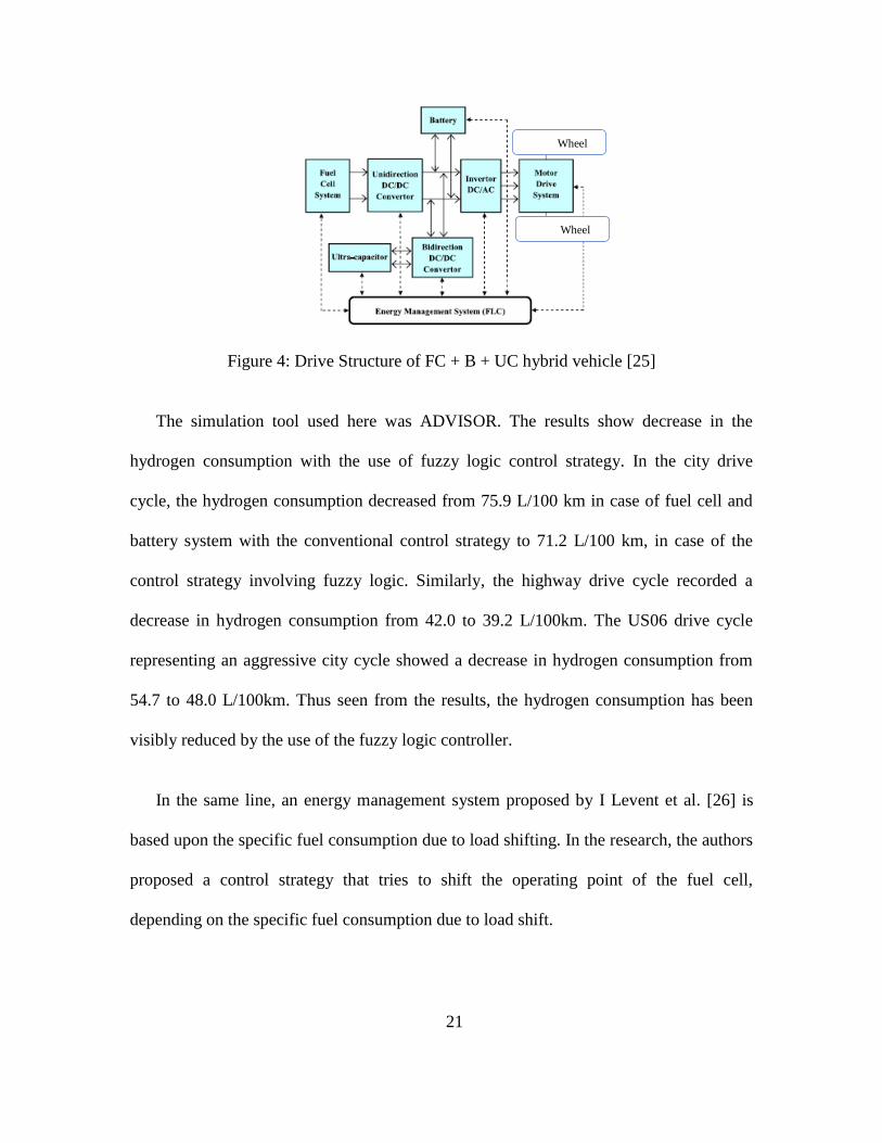
21
Figure 4: Drive Structure of FC + B + UC hybrid vehicle [25]
The simulation tool used here was ADVISOR. The results show decrease in the
hydrogen consumption with the use of fuzzy logic control strategy. In the city drive
cycle, the hydrogen consumption decreased from 75.9 L/100 km in case of fuel cell and
battery system with the conventional control strategy to 71.2 L/100 km, in case of the
control strategy involving fuzzy logic. Similarly, the highway drive cycle recorded a
decrease in hydrogen consumption from 42.0 to 39.2 L/100km. The US06 drive cycle
representing an aggressive city cycle showed a decrease in hydrogen consumption from
54.7 to 48.0 L/100km. Thus seen from the results, the hydrogen consumption has been
visibly reduced by the use of the fuzzy logic controller.
In the same line, an energy management system proposed by I Levent et al. [26] is
based upon the specific fuel consumption due to load shifting. In the research, the authors
proposed a control strategy that tries to shift the operating point of the fuel cell,
depending on the specific fuel consumption due to load shift.
Wheel
Wheel
22
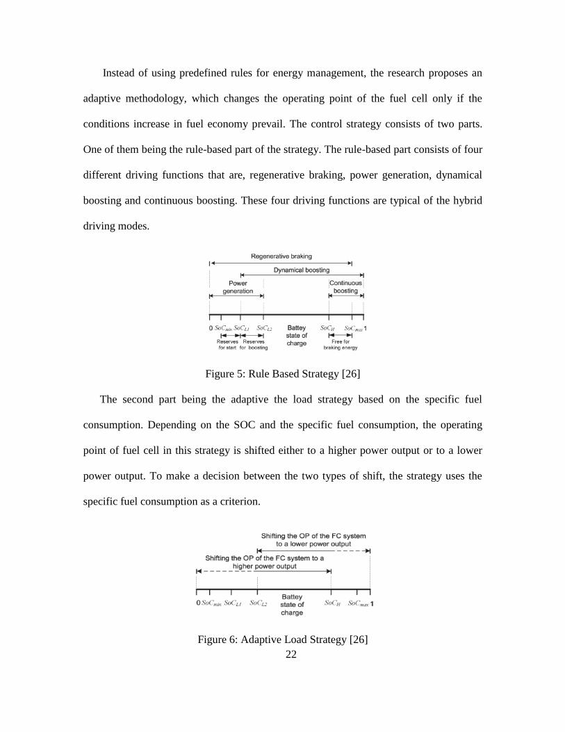
Instead of using predefined rules for energy management, the research proposes an
adaptive methodology, which changes the operating point of the fuel cell only if the
conditions increase in fuel economy prevail. The control strategy consists of two parts.
One of them being the rule-based part of the strategy. The rule-based part consists of four
different driving functions that are, regenerative braking, power generation, dynamical
boosting and continuous boosting. These four driving functions are typical of the hybrid
driving modes.
Figure 5: Rule Based Strategy [26]
The second part being the adaptive the load strategy based on the specific fuel
consumption. Depending on the SOC and the specific fuel consumption, the operating
point of fuel cell in this strategy is shifted either to a higher power output or to a lower
power output. To make a decision between the two types of shift, the strategy uses the
specific fuel consumption as a criterion.
Figure 6: Adaptive Load Strategy [26]

23
3: METHODOLOGY
This section of the report sheds light on the hardware setup, software configurations
and modelling. It highlights the concepts used in modelling as well as explains in details
the procedure used for performing the fuel cell HiL.
Software Setup
MATLAB/SIMULINK© [27] software platform was used in order to model the
vehicle. MATLAB© meaning Matrix Laboratory is a multi-paradigm programming
language developed by MathWorks Inc. It allows numerical computing including matrix
calculations, algorithm implementation and provides for an interface between other
programming languages such as C, C++, Java, etc.
Simulink© [27] is a graphical programming tool package associated with Matlab©. It
provides block diagrams for various mathematical operations, which can be used for
development of simulation programs. It is a powerful tool in ways it can drive Matlab©
or be run by it depending on the type of application. It is widely been used by researchers
for simulating and modelling dynamic systems for testing purposes.
Simulink© has been used not only for building and for simulating models, but also
managing projects and analyzing results. It can also be connected to hardware for real
time testing. One of the major achievements of Simulink© has been the ability to model
non-linear systems. A non-linear system is the one in which, the outputs of the system are
not in direct proportion to the system inputs.

24
Vehicle Modelling
A bottom-up approach was used for modelling the vehicle system. The major
components were modeled and put together for data flow. This type of approach is
helpful in building complex system such as this application. The major vehicle
components related to fuel cell vehicle included the fuel cell and electric motor system,
electric motor gearbox, wheels, brakes and the controller for the fuel cell and the electric
motor system.
A top level block diagram is shown in the following figure.
Figure 7: Top Level: Vehicle Modeling
The top levels consist of the driving cycles, driver block, powertrain block and the
vehicle dynamics block as shown. The driver block takes the driving cycles as the input
and calculates the acceleration or brake required to achieve this driving profile based on
the current vehicle velocity. The powertrain block consists of the vehicle powertrain
including the fuel cell and electric motor system, the gearbox, wheels and brakes. The
output of the powertrain block is the tractive force required to propel the vehicle.

25
The vehicle dynamics block takes into consideration the forces acting on the vehicle.
Each of these blocks consist of sub systems. These subsystems are explained in detail in
the following sections. The ‘clock’ block is used for output of the simulation time and is
stored in the name of a variable ‘t’ in the workspace.
Driving Cycle
The input to the model was given in form of pre-defined standard driving cycles. A
drive cycle is a series of data representing the velocity of the vehicle versus the time.
These drive cycles have been developed by different countries according to the road load
conditions pertaining to that region and the standard driving profiles. The drive cycles are
used to evaluate various vehicle performance parameters such as fuel consumption,
vehicle emissions, fuel economy, etc. The model used three types of driving cycles,
concerned with the driving profiles found majorly in the United States.
The US Environmental Protection Agency (EPA) [28] has formulated the drive cycles
and they serve as the base of comparison for testing various types of automotive system.
The Federal Urban Driving Schedule (FUDS), also called the Urban Dynamometer
Driving Schedule (UDDS) or the city test as it portraits the city driving conditions. This
driving cycle runs over a distance of 7.45 miles in a time of 1369 seconds with an
average speed of 19.59 mph. The profile represents frequent stops imitating the city
driving conditions. The maximum speed the vehicle achieves is limited to 55 mph
considering the traffic laws effective in the US.
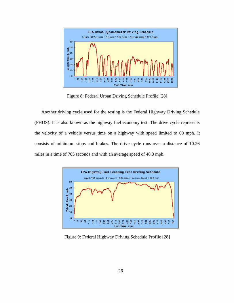
26
Figure 8: Federal Urban Driving Schedule Profile [28]
Another driving cycle used for the testing is the Federal Highway Driving Schedule
(FHDS). It is also known as the highway fuel economy test. The drive cycle represents
the velocity of a vehicle versus time on a highway with speed limited to 60 mph. It
consists of minimum stops and brakes. The drive cycle runs over a distance of 10.26
miles in a time of 765 seconds and with an average speed of 48.3 mph.
Figure 9: Federal Highway Driving Schedule Profile [28]

27
US06 driving schedule also known as supplemental FTP (Federal Test Procedure) is a
supplement drive cycle to the FUDS. It is a more aggressive representation of city driving
conditions. It consists of high acceleration as compared to the FUDS. It has less frequent
stops but higher speeds in comparison to FUDS. It runs over a distance of 8.01 miles, in a
time of 596 seconds, with an average speed of 48.37 mph.
Figure 10: Aggressive Urban Driving Schedule Profile [28]
Lastly, an acceleration test is performed to evaluate the acceleration capability of the
fuel cell system. The test runs over a time of 100 seconds and draws maximum power
from the fuel cell.
Figure 11: Acceleration Test Profile
0 10 20 30 40 50 60 70 80 90 1000
20
40
60
80
100
120
140Acceleration Test Velocity Profile
Time [s]
Ve
hic
le V
elo
city [
mp
h]
Desired Speed of vehicle
Actual Speed of vehicle
28
A ‘Source Block’ is used to output the values of driving cycles. The source block is a
repeating table block, which outputs the values specified in a table with respect to the
instantaneous time. It consists of two columns, one being the time and the other being the
specified parameter, which the user wants to output.
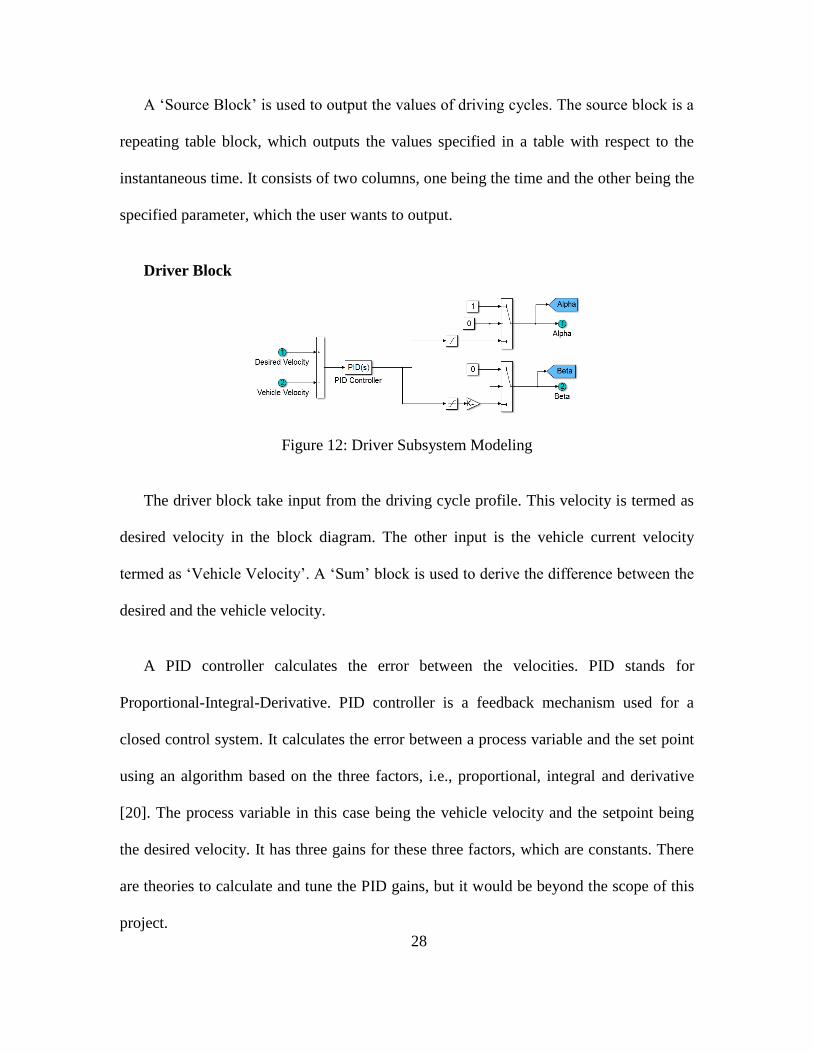
Driver Block
Figure 12: Driver Subsystem Modeling
The driver block take input from the driving cycle profile. This velocity is termed as
desired velocity in the block diagram. The other input is the vehicle current velocity
termed as ‘Vehicle Velocity’. A ‘Sum’ block is used to derive the difference between the
desired and the vehicle velocity.
A PID controller calculates the error between the velocities. PID stands for
Proportional-Integral-Derivative. PID controller is a feedback mechanism used for a
closed control system. It calculates the error between a process variable and the set point
using an algorithm based on the three factors, i.e., proportional, integral and derivative
[20]. The process variable in this case being the vehicle velocity and the setpoint being
the desired velocity. It has three gains for these three factors, which are constants. There
are theories to calculate and tune the PID gains, but it would be beyond the scope of this
project.

29
The PID controller determines the error between the velocities, which then
determines either acceleration or brake to be applied to achieve the target. If the error
falls in the negative category, it is applied as a brake command and vice-versa. An
algorithm is applied to identify the state of the values being output by the PID controller.
The algorithm uses ‘Saturation’ and ‘Switch’ blocks to do so. A ‘Saturation’ block
consists of two input values namely, the upper saturation value and the lower saturation
value. The user can input these values and limit the output to be bound between them.
The values that fall between the lower and upper values are given as output and rest are
discarded.
The ‘Switch’ block tests the input against a certain condition. The outputs of this
block are given as ‘Alpha’ and ‘Beta’, representing the acceleration and brake
commands.
Powertrain Sub Model
The powertrain block takes into consideration the alpha and beta commands given by
the driver block and requests the corresponding tractive force to be provided by the fuel
cell. Figure 13 shows the top level of the powertrain block.
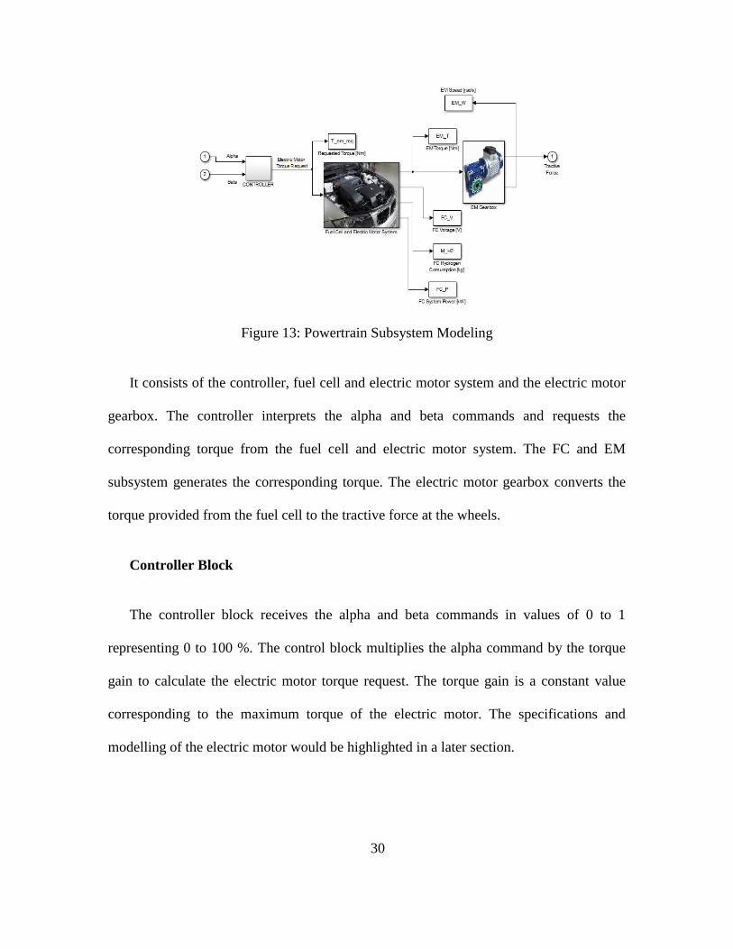
30
Figure 13: Powertrain Subsystem Modeling
It consists of the controller, fuel cell and electric motor system and the electric motor
gearbox. The controller interprets the alpha and beta commands and requests the
corresponding torque from the fuel cell and electric motor system. The FC and EM
subsystem generates the corresponding torque. The electric motor gearbox converts the
torque provided from the fuel cell to the tractive force at the wheels.
Controller Block
The controller block receives the alpha and beta commands in values of 0 to 1
representing 0 to 100 %. The control block multiplies the alpha command by the torque
gain to calculate the electric motor torque request. The torque gain is a constant value
corresponding to the maximum torque of the electric motor. The specifications and
modelling of the electric motor would be highlighted in a later section.
31
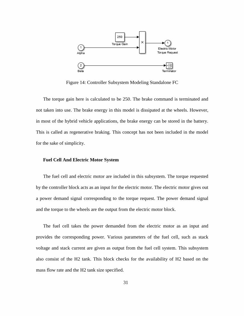
Figure 14: Controller Subsystem Modeling Standalone FC
The torque gain here is calculated to be 250. The brake command is terminated and
not taken into use. The brake energy in this model is dissipated at the wheels. However,
in most of the hybrid vehicle applications, the brake energy can be stored in the battery.
This is called as regenerative braking. This concept has not been included in the model
for the sake of simplicity.
Fuel Cell And Electric Motor System
The fuel cell and electric motor are included in this subsystem. The torque requested
by the controller block acts as an input for the electric motor. The electric motor gives out
a power demand signal corresponding to the torque request. The power demand signal
and the torque to the wheels are the output from the electric motor block.
The fuel cell takes the power demanded from the electric motor as an input and
provides the corresponding power. Various parameters of the fuel cell, such as stack
voltage and stack current are given as output from the fuel cell system. This subsystem
also consist of the H2 tank. This block checks for the availability of H2 based on the
mass flow rate and the H2 tank size specified.

32
Figure 15: Fuel Cell and Electric Motor Subsystem Modeling
Fuel Cell Subsystem
Keeping in mind the performance characteristics of a light duty vehicle, an 80 kW
fuel cell system is modelled. The modelling of the fuel cell required various parameters
related to the fuel cell characteristics. The following assumptions corresponding to the 80
kW fuel cell system have been used.
PARAMETER DESCRIPTION VALUE
Area.FC Cell Area [cm2] 420
N_FC Number of stack cells 380
H2_FC Hydrogen Utilization Factor 0.9
Lhv_FC Lower Heating Value of Fuel [kJ/kg] 11300
Table 3: Fuel Cell Parameters [24, 30]
A cell polarization curve is used to plot the stack voltage from the current density and
the cathode pressure. The cathode pressure is obtained from the corresponding current
demand from the fuel cell.
33
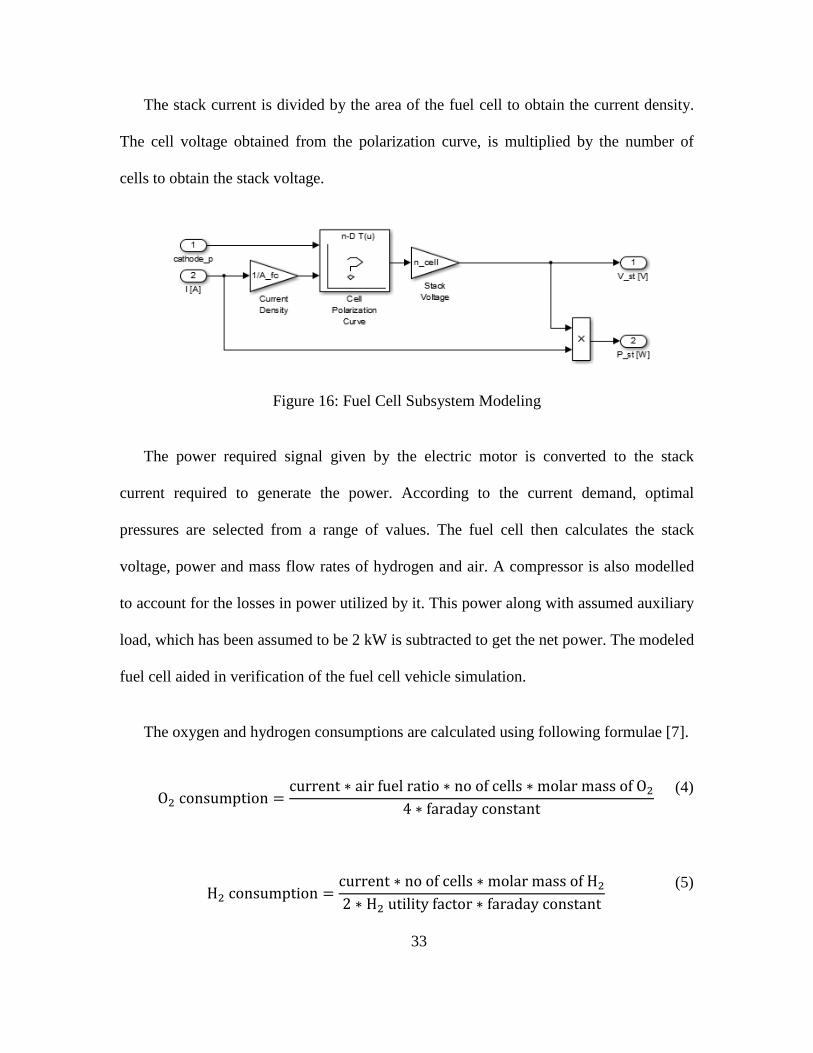
The stack current is divided by the area of the fuel cell to obtain the current density.
The cell voltage obtained from the polarization curve, is multiplied by the number of
cells to obtain the stack voltage.
Figure 16: Fuel Cell Subsystem Modeling
The power required signal given by the electric motor is converted to the stack
current required to generate the power. According to the current demand, optimal
pressures are selected from a range of values. The fuel cell then calculates the stack
voltage, power and mass flow rates of hydrogen and air. A compressor is also modelled
to account for the losses in power utilized by it. This power along with assumed auxiliary
load, which has been assumed to be 2 kW is subtracted to get the net power. The modeled
fuel cell aided in verification of the fuel cell vehicle simulation.
The oxygen and hydrogen consumptions are calculated using following formulae [7].
O2 consumption =
current ∗ air fuel ratio ∗ no of cells ∗ molar mass of O2
4 ∗ faraday constant
(4)
H2 consumption =
current ∗ no of cells ∗ molar mass of H2
2 ∗ H2 utility factor ∗ faraday constant
(5)

34
Where,
Air fuel ratio = 2
Molar mass of 02 = 32 X 10-3 kg
Molar mass of H2 = 2 X 10⁻³ kg
Faraday constant = 96485
Table 4: Fuel Cell Constants
Electric Motor Subsystem
The model has input of Acceleration and Braking, which is multiplied with maximum
motor torque respectively. This total Torque is summed up and is stored in variable
named ‘EM_T_req’ this is the electric motor torque request which is fed as input to the
saturation dynamic block where this signals are processed with other signals of electric
motor torque min and max curves respectively feed to the saturation block. The saturation
block after processing these three signals produces an output which is electric motor
torque stored in variable name ‘EM_trq’ in the workspace.
Meanwhile the electric motor torque request is also fed as an input signal to the
electric motor efficiency map for the current electric motor being used in vehicle model.
The other input to the efficiency map is the ‘EM_trq’ the output torque of electric motor.
As an output, we get the electric motor efficiency stored in variable name “EM_eff”.This
output signal “EM_trq” is fed to a switch, which decides whether the motor is consuming
power or producing power.
35
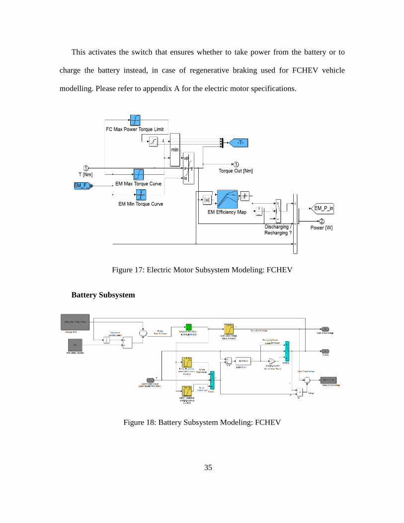
This activates the switch that ensures whether to take power from the battery or to
charge the battery instead, in case of regenerative braking used for FCHEV vehicle
modelling. Please refer to appendix A for the electric motor specifications.
Figure 17: Electric Motor Subsystem Modeling: FCHEV
Battery Subsystem
Figure 18: Battery Subsystem Modeling: FCHEV
36
The figure shows the battery model subsystem used or hybridizing the fuel cell
vehicle. Battery State of Charge (SOC) is calculated by dividing total battery capacity of
the battery from used battery capacity, which is derived by integrating current coming out
of the battery. Power required by electric motor is equal to power output from the battery;
hence, power input of motor is used to determine output voltage and current of battery.
The SOC value is used to determine open circuit voltage of battery, and Internal
Resistance of battery while charging as well as discharging. These all values are given in
a table and Lookup is used to get corresponding output variables w.r.t SOC. Open circuit
voltage can be obtained directly using lookup for Open circuit Voltage corresponding to
SOC.
Switch is used to determine the battery resistance for charging/discharging scenarios.
Motor power is used to determine the output of the switch. If motor power is positive,
discharging resistance will pass through the switch, and if motor power is negative,
charging resistance will be passed.
Output from the switch is divided from Motor Power and taking its square root gives
us total current flowing in the battery for both charging and discharging [29].
√
𝑃
𝑅 = √
𝑅𝑖2
𝑅 = i (Current)
(6)
Voltage across electric motor (i.e. closed circuit voltage of battery) is obtained by
dividing battery current with corresponding charging/discharging resistance and
subtracting this voltage from open circuit voltage of battery.

37
These results are for a single battery module. Battery system for the FCHEV consist
of a stack of battery cells in series and parallel. To obtain voltage/current for complete
pack, the voltage and current was scaled accordingly by multiplying voltage with number
of battery modules in series, and multiplying current with number of battery modules in
parallel. Please refer to appendix A for the battery specifications.
Control Strategy Implementation
LOAD FOLLOWING CONTROL STRATEGY
The load following control strategy works on the principle of identifying the power
demand by the electric motor and responding with the power from the battery or the fuel
cell [32]. This control strategy works directly based on the power demand by the electric
motor system. Although many variations of this control strategy have been studied, the
basic principle remains unchanged.
For the purpose of this experiment, a control strategy involving the division of power
demand of the electric motor system according to the magnitude has been developed.
Low loads with magnitude of 5kw or less are sufficed by the energy storage system,
which is the battery in this case. The loads in the range of 5 kW to 25kw are powered
with combined power from the battery and the fuel cell. Loads greater than 25kw are
powered solely by the fuel cell system.
38
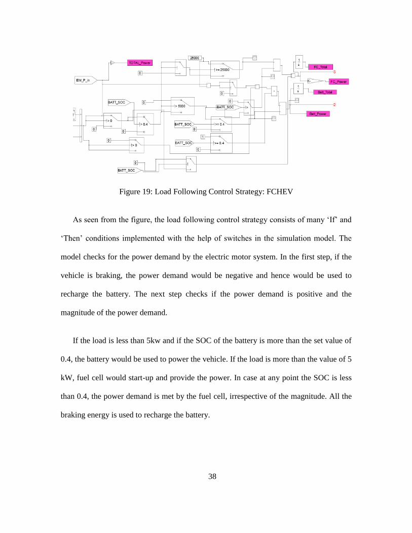
Figure 19: Load Following Control Strategy: FCHEV
As seen from the figure, the load following control strategy consists of many ‘If’ and
‘Then’ conditions implemented with the help of switches in the simulation model. The
model checks for the power demand by the electric motor system. In the first step, if the
vehicle is braking, the power demand would be negative and hence would be used to
recharge the battery. The next step checks if the power demand is positive and the
magnitude of the power demand.
If the load is less than 5kw and if the SOC of the battery is more than the set value of
0.4, the battery would be used to power the vehicle. If the load is more than the value of 5
kW, fuel cell would start-up and provide the power. In case at any point the SOC is less
than 0.4, the power demand is met by the fuel cell, irrespective of the magnitude. All the
braking energy is used to recharge the battery.
39
If the load demand is more than 25 kW, the fuel cell would provide the sole power
and the battery would recharge. At every step of the process, the battery SOC is checked
for the condition of 0.4 before drawing power from the battery. The load range of zero -
25 kW covers the 70% loading during the standard driving cycle conditions. Thus
through this control strategy, the fuel cell hydrogen consumption can be reduced.
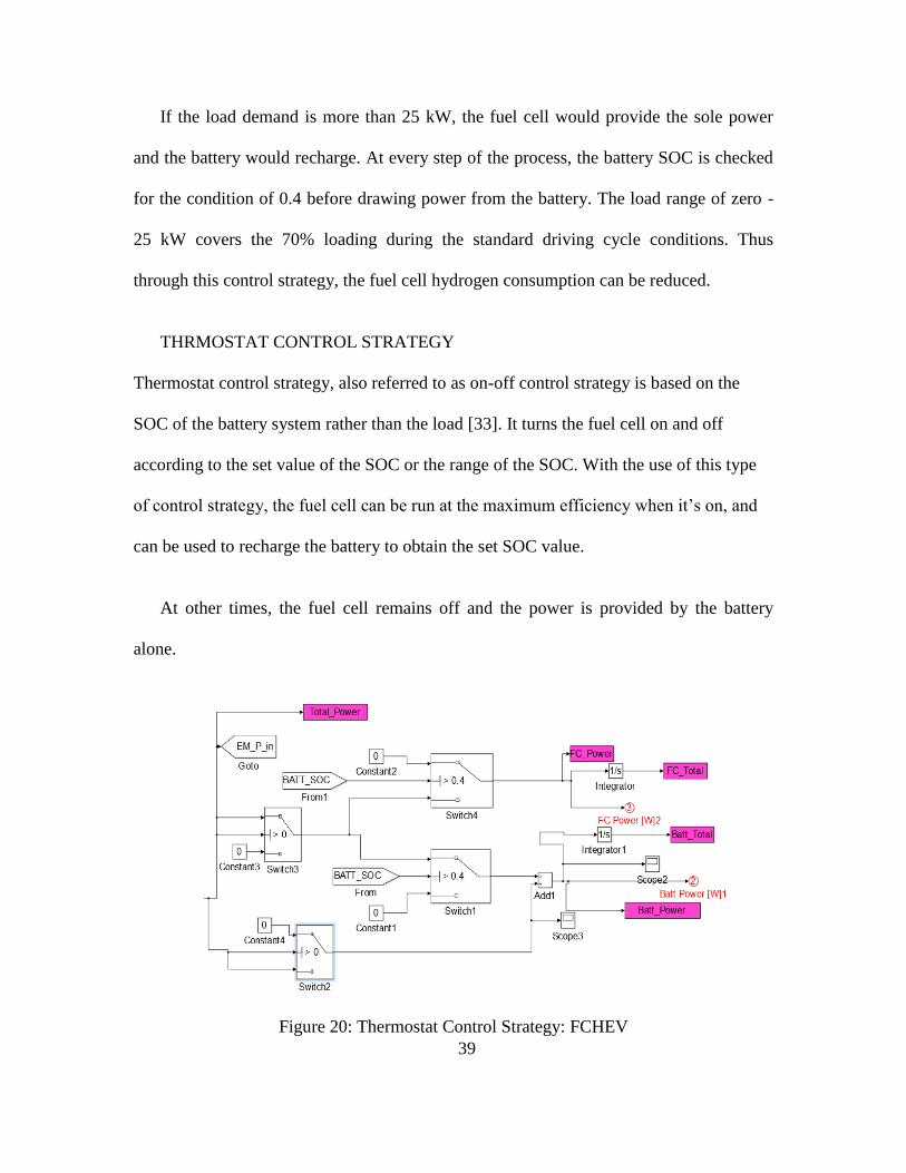
THRMOSTAT CONTROL STRATEGY
Thermostat control strategy, also referred to as on-off control strategy is based on the
SOC of the battery system rather than the load [33]. It turns the fuel cell on and off
according to the set value of the SOC or the range of the SOC. With the use of this type
of control strategy, the fuel cell can be run at the maximum efficiency when it’s on, and
can be used to recharge the battery to obtain the set SOC value.
At other times, the fuel cell remains off and the power is provided by the battery
alone.
Figure 20: Thermostat Control Strategy: FCHEV

40
In the same line with the load following control strategy, this strategy utilizes the
braking energy as regenerative braking to be stored in the battery. In the next step, the
system checks if the battery SOC is above the set limit, in this case 0.4. If the SOC is
greater than the value, the power is provided by the battery system and the fuel cell
remains off. If not, the fuel is turned on to recharge the battery and provide the required
power demand. This minimizes the use of fuel cell and thus reduces the hydrogen
consumption.
41
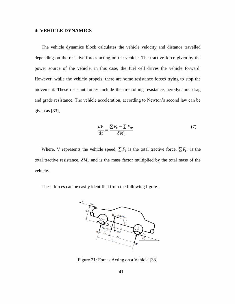
4: VEHICLE DYNAMICS
The vehicle dynamics block calculates the vehicle velocity and distance travelled
depending on the resistive forces acting on the vehicle. The tractive force given by the
power source of the vehicle, in this case, the fuel cell drives the vehicle forward.
However, while the vehicle propels, there are some resistance forces trying to stop the
movement. These resistant forces include the tire rolling resistance, aerodynamic drag
and grade resistance. The vehicle acceleration, according to Newton’s second law can be
given as [33],
𝑑𝑉
𝑑𝑡=
∑ 𝐹𝑡 − ∑ 𝐹𝑡𝑟
𝛿𝑀𝑣
(7)
Where, V represents the vehicle speed, ∑ 𝐹𝑡 is the total tractive force, ∑ 𝐹𝑡𝑟 is the
total tractive resistance, 𝛿𝑀𝑣 and is the mass factor multiplied by the total mass of the
vehicle.
These forces can be easily identified from the following figure.
Figure 21: Forces Acting on a Vehicle [33]

42
Rolling Resistance
The rolling resistance is the caused by the resistance between the tires and surface,
due the tire materials. When the tire is rolling, a deflection in carcass causes a non-
symmetric distribution of reaction forces. This creates a difference in the amount of force
exerted on the forward and backward parts of the tire in motion. This difference in forces
tends to create a moment on the tire, which opposes its motion. This rolling resistance
moment can be expressed as [33]
𝑇𝑟 = 𝑃𝑎 (8)
To counter this resistance, the force needed at the center of the wheels, is given as
[33],
𝐹 =
𝑇𝑟
𝑟𝑑=
𝑃𝑎
𝑟𝑑= 𝑃𝑓𝑟
(9)
Where, 𝑟𝑑 is the effective radius of the tire, 𝑓𝑟 is the rolling resistance coefficient, P is
the normal load, acting on the center of the wheel. When the vehicle drives on a slope
road, the component of the force acting perpendicular to the surface of the road is
expressed as [33],
𝐹𝑟 = 𝑃𝑓𝑟𝑐𝑜𝑠 (10)
Where, 𝐹𝑟 is the rolling resistance, and ∝ is the slope of the road. The rolling
resistance coefficient, 𝑓𝑟 depends on various factors including, tire material, tire
temperature, tire structure and geometry, road material, etc.

43
Based on experimental results, many rolling resistance coefficient values have
been formulated to be used under different conditions. For the purpose of this project, a
value of 0.015 has been assumed based on the car tires running on concrete or asphalt.
Also, the force can be expressed in terms of mass and acceleration due to gravity,
assumed 9.8 m /s2. Thus the final equation is [33],
𝐹𝑟 = 𝑀𝑔𝑓𝑟𝑐𝑜𝑠 ∝ (11)
Aerodynamic Drag
When a vehicle travels at a particular speed, the air surrounding the vehicle exerts a
certain type of resistive motion on it. This is called as aerodynamic drag. This kind of
drag results from the shape of the vehicle and the friction caused by the skin or material
and texture of the outer body. As the vehicle moves forward at a speed, the air in front of
the vehicle cannot move as fast at the car, thus exerting some resistance. Also, the space
left behind the car as it moves, creates and area of low pressure thus increasing the
resistance. This is mainly caused by the shape of the vehicle.
The aerodynamic drag can be expressed as a function of vehicle speed𝑉, air density𝛿,
vehicle frontal area 𝐴𝑓 as [33],
𝐹𝑎 =
1
2𝛿𝐴𝑓𝐶𝑑𝑉2
(12)
Where, 𝐶𝑑is the aerodynamic drag coefficient. It depends on the vehicle shape.

44
Grade Resistance
Another type of resistance acting on a vehicle is the grade resistance. This resistance
acts whenever the vehicle moves on a slope. The grade resistance acts in the downward
direction appendicular to the car. It acts in two ways, i.e., it resists the motion, when the
vehicle climbs, whereas, it assists the motion, when the vehicle descends on a slope.
The grading resistance is a function of vehicle mass, acceleration due to gravity and
the angle of slope. It is expressed as [33],
𝐹𝑔 = 𝑀𝑔𝑠𝑖𝑛 ∝ (13)
For the purpose of this project, the values of the variables have been assumed
depending on the generalized use of the vehicle. The grade is assumed to be zero, for
simplicity.
Parameter Value
Tire Radius, 𝑟𝑑 0.3305 m
Vehicle Mass, M 2000 kg
Gravitational Acceleration, g 9.8 m/s2
Air Density, 𝛿 1.29
Frontal Area, 𝐴𝑓 2.82 m2
Aerodynamic Drag Coefficient, 𝐶𝑑 0.416
Table 5: Vehicle Parameters [33]

45
Thus, the total tractive force required to move the vehicle could be given as,
𝑆𝑢𝑚𝑚𝑎𝑡𝑖𝑜𝑛 𝑜𝑓 𝐹𝑜𝑟𝑐𝑒𝑠 = 𝐹𝑡𝑟 − 𝐹𝑟 − 𝐹𝑎 − 𝐹𝑔 (14)
Therefore, 𝐹𝑡𝑟 − 𝑚𝑔𝐶𝑟𝑟 −1
2𝜌 𝐶𝑑𝐴𝑓𝑉2 − 𝑚𝑔𝑠𝑖𝑛𝛼 = 𝑚𝑒𝑓𝑓 ∗ 𝑎𝑐𝑐 (15)
Where, meff is the effective mass of the vehicle, as an effect of the rotating
components in the powertrain, assumed to be 1.04 *m.
Thus, the tractive effort required can be given as [33],
𝐹𝑡𝑟 = 𝑚𝑔𝐶𝑟𝑟 +
1
2𝜌𝐶𝑑𝐴𝑓𝑉2 + 𝑚𝑒𝑓𝑓 ∗ 𝑎𝑐𝑐
(16)
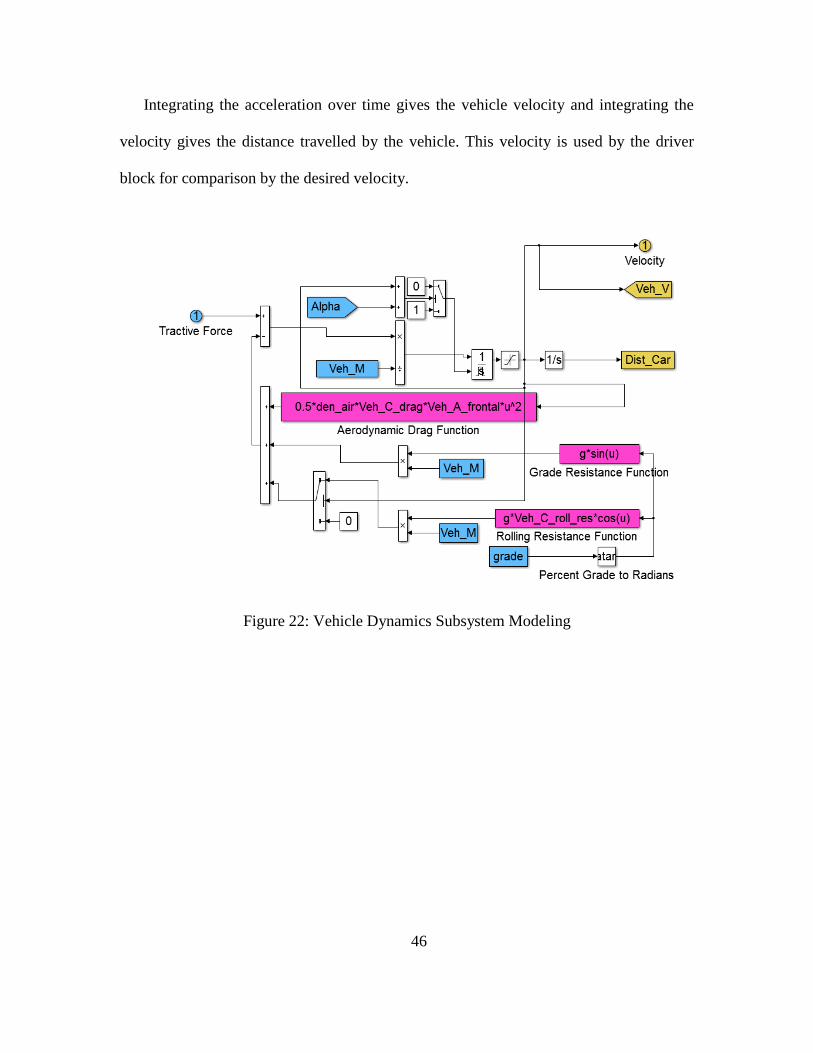
Model Description
In the model, the three resistive forces i.e. aerodynamic drag, grade resistive force
and rolling resistance are together deducted from the net tractive force to produce an
output tractive force.
The aerodynamic drag function is calculated according to the equation with the
inputs, air density, vehicle frontal area, coefficient of drag and vehicle velocity. The
grade resistance function is calculated according to equation using the inputs of
gravitational acceleration and angle of slope. The vehicle mass then multiplies this
function. The rolling resistance function is calculated using equation and inputs of
gravitational acceleration, coefficient of rolling resistance and angle of slope. The vehicle
mass then multiplies this function.
46
Integrating the acceleration over time gives the vehicle velocity and integrating the
velocity gives the distance travelled by the vehicle. This velocity is used by the driver
block for comparison by the desired velocity.
Figure 22: Vehicle Dynamics Subsystem Modeling

47
5: HARDWARE SETUP
Developed by National Instruments Inc., the NI PXIe-6341 is used as a high-speed
real time controller with Analog and Digital I/O’s data acquisition (DAQ) system. This
DAQ is used along with the controller chassis to acquire and communicate data with
other hardware components. The power required from the FC according to the drive
cycle, is considered to be the driving factor of the system under consideration. The power
requirement is conveyed to the FC through the real time controllable DC electronic load.
The closed loop feedback is implemented based on the fuel cell stack operating
temperature. Two surface mount thermocouples (TC’s) of type K, were used to obtain the
temperature readings from the FC stack surface.
Figure 23: Basic hardware data flow for the closed-loop FCV HiL.

48
Hardware Components
NI PXI
PXI is a PC based measurement and automation system platform developed by
National Instruments. It combines the features of PCI electrical-bus with other
specialized synchronization buses. A single PXI system is capable of replacing the real
time target, PLC and the control PC. The NI PXIe-1071 chassis is a 4 slot PXI Express
chassis. It provides high speed bandwidth of up to 1 GB/s per slot. It supplements this
feature with 10 MHz and 100 MHz reference clocks. The PXIe-1071 used for the project
was aided with 2 data acquisition systems, namely PXIe-6341 and PXI- 6722 controllers.
The PXIe-6341 is an X series data acquisition system with the capability of providing
16 analog inputs and 2 analog outputs. The PXI 6722 is an eight channel digital
input/output controller. The PXIe-6341 needed to be connected with SCB-68A connector
block for the purpose of transmitting and receiving analog signals.
AMREL PEL SEIRES 300-60-60
The DC electronic load used for controlling the fuel cell was chosen to be the
AMREL PEL 300-60-60. It is a real time programmable DC electronic load
manufactured by American Reliance Limited, with a power capability of 300 W. Though
having a lower power capability than desired application, the scaling of the fuel cell aided
in acquiring the results.
49
Moreover, the DC e-Load needed to be real time programmable, in the sense that the
power drawn by the e-Load needed to be controlled dynamically by the PXI.
NEXA HELIOCENTRIS 1.2 FUEL CELL
The FCVHiL was performed on the Nexa Heliocentris 1.2 fuel cell, comprising of
FCgenTM 1020 ACS fuel cell stack, manufactured by Ballard Energy Systems. The fuel
cell is a PEM (Proton Exchange Membrane) type. It requires hydrogen and air as fuels for
producing electricity. The fuel cell has a power output capability of 1.2 kW, with a rated
current of 52 A and rated voltage of 24 V. The operational temperature of the fuel cell
varies between 5 and 40 °C. It is an air-cooled type of fuel cell with a fan accommodated
at the rear for cooling.
In PEM type of fuel cells, the hydrogen reacts with oxygen from air to produce water
and electricity. The membrane is an ion exchange membrane. PEM fuel cells have the
advantages of producing higher power density and capable of faster start-ups to name a
few.
HIL Methodology Implementation
The model implementation was done through MATLAB/SIMULINK© and then
interfaced with LABVIEW© using tools like Simulation interface toolkit (SIT) for real
time implementation. Labview© stands for Laboratory Virtual Instrument Engineering
Workbench, is a software platform developed by NI.
50
Labview© aids in data acquisition, industrial automation and instrument control on a
variety of platforms including Microsoft Windows, Linux, Mac OS X, etc. Labview© is
programmed using a dataflow programming language, G. The user interface consists of
blocks with various inbuilt operations that can be connected using virtual wires.
Labview© acts as an interface between SIMULINK© and the real fuel cell using an
analog input/output system I/O. With the use of PID controller logic to minimize the
errors, efficient model execution can be obtained.
The vehicle model developed in Simulink© is compiled into an executable ‘DLL’
format for communication with Labview©. DLL is a Dynamic Library Link format
developed by Microsoft for intercommunication between various software platforms. The
communication between Simulink© and Labview© required software compatibility
between the two platforms, not only in terms of the versions, but also in terms of the C
programming software used by Simulink©.
A virtual panel constructed in labview© environment gives a complete control of the
simulation model and works with the PXI controller to send and acquire analog signals to
and from the model. The power required from the FC is scaled from 80KW simulated
model to 300 W.
PXI directly controls the fuel cell test stand in real time with its key software features.
The use of SIMULINK (MATLAB©) for controlling and monitoring the simulation and
LABVIEW© as a subordination tool provides an arch for the real time control of the fuel
cell test stand.
51
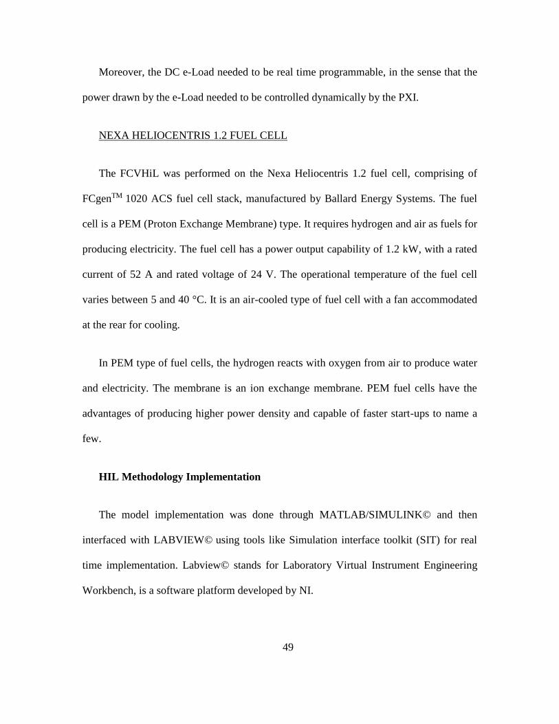
The closed HiL implementation required replacing the modelled fuel cell with the real
hardware. The power request from the electric motor was taken out as an analog output
signal through the Labview ©. This signal was used to drive the e-Load to draw power
from the fuel cell. The maximum power that can be drawn by the DC load is 300 W.
Analog voltage signals were used to control the level of power drawn in real time. Using
analog voltage signals for communication aided in the simplicity of test bench, as
compared to traditional GPIB or RS232.
Figure 24: HiL Hardware Setup
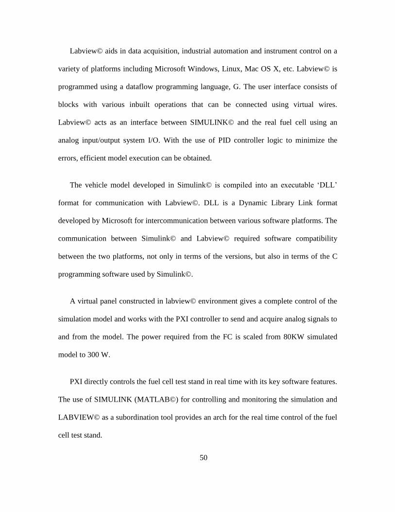
The figure shows the implantation of the FCVHiL. Temperature was chosen to be the
limiting factor (constraint) for the fuel cell due to its importance relating to the working
of fuel cells, especially PEM FC’s. As the temperature of the fuel cell stack increases, the
efficiency decreases. IN PEM FC’s, hydrogen and oxygen react to produce water and
electricity along with heat.
52
The heat produced can be utilized for evaporation of the water produced and thus
given out of the system. However, the amount of heat produced is greater. This results in
heating of the stack and in turn the membrane. As the temperature of the membrane
increases, the conductivity decreases, thus decreasing the efficiency for chemical
reactions.
As shown in Figure 25, one TC is placed at the right corner of the stack and other at
the center, to the point accessible. These temperatures are communicated back to the
simulation model as analog voltage signals through NI DAQ and controller. The cut-off
temperature in the model is set to a higher value of 45°C, as the NEXA FC system is
comprised of a built in temperature shut-off system at 40°C operating temperature, for the
sake of system verification.
Figure 25: Thermocouple Placement
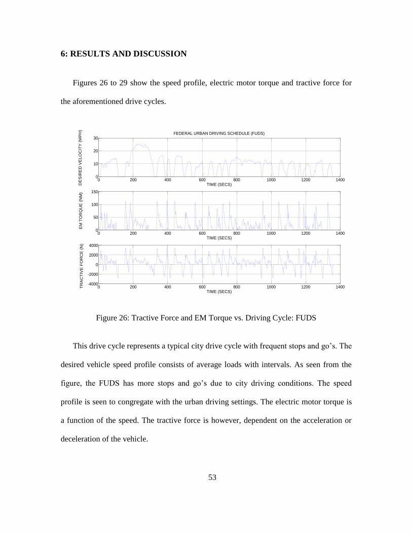
53
6: RESULTS AND DISCUSSION
Figures 26 to 29 show the speed profile, electric motor torque and tractive force for
the aforementioned drive cycles.
Figure 26: Tractive Force and EM Torque vs. Driving Cycle: FUDS
This drive cycle represents a typical city drive cycle with frequent stops and go’s. The
desired vehicle speed profile consists of average loads with intervals. As seen from the
figure, the FUDS has more stops and go’s due to city driving conditions. The speed
profile is seen to congregate with the urban driving settings. The electric motor torque is
a function of the speed. The tractive force is however, dependent on the acceleration or
deceleration of the vehicle.
0 200 400 600 800 1000 1200 14000
10
20
30
TIME (SECS)DE
SIR
ED
VE
LO
CIT
Y (
MP
H)
FEDERAL URBAN DRIVING SCHEDULE (FUDS)
0 200 400 600 800 1000 1200 14000
50
100
150
TIME (SECS)
EM
TO
RQ
UE
(N
M)
0 200 400 600 800 1000 1200 1400-4000
-2000
0
2000
4000
TIME (SECS)
TR
AC
TIV
E F
OR
CE
(N
)
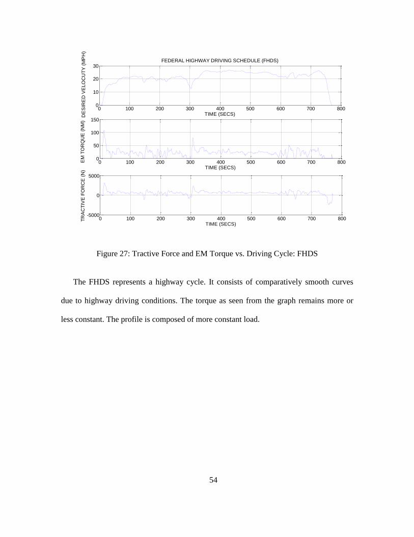
54
Figure 27: Tractive Force and EM Torque vs. Driving Cycle: FHDS
The FHDS represents a highway cycle. It consists of comparatively smooth curves
due to highway driving conditions. The torque as seen from the graph remains more or
less constant. The profile is composed of more constant load.
0 100 200 300 400 500 600 700 8000
10
20
30
TIME (SECS)DE
SIR
ED
VE
LO
CU
TY
(M
PH
)
FEDERAL HIGHWAY DRIVING SCHEDULE (FHDS)
0 100 200 300 400 500 600 700 8000
50
100
150
TIME (SECS)
EM
TO
RQ
UE
(N
M)
0 100 200 300 400 500 600 700 800-5000
0
5000
TIME (SECS)
TR
AC
TIV
E F
OR
CE
(N
)

55
Figure 28: Tractive Force and EM Torque vs. Driving Cycle: US06
The US06 represents aggressive urban cycle. It comprises of more aggressive
accelerations than the highway drive cycle. It can said to be a combination of the city and
highway cycles with higher acceleration rates at the beginning and at the end. One thing
to be noted here is that, in a hybrid energy system, the fuel cell can supply power for only
base loads. The acceleration peaks cannot be provided by the fuel cell system. For this
purpose, an alternative energy source such as a battery is used to supply energy demands
for high acceleration peaks. In addition, regenerative braking can be taken into account
for charging the battery when brakes are applied. These considerations can account for
higher performance of fuel cells
0 100 200 300 400 500 6000
20
40
TIME (SECS)
DE
SIR
ED
VE
LO
CIT
Y (
MP
H)
US 06
0 100 200 300 400 500 6000
100
200
TIME (SECS)
EM
TO
RQ
UE
(N
M)
0 100 200 300 400 500 600-5000
0
5000
10000
TIME (SECS)TR
AC
TIV
E F
OR
CE
(N
)

56
Figure 29: Tractive Force and EM Torque vs. Driving Cycle: Acc Test
The acceleration test comprises of maximum load for a specific period of time. This
test plays a vital role from the efficiency test and temperature test point of view. As seen
from the speed profile, the load is increased to maximum and kept at that point for a
specific period of time.
These four drive cycles would embody all the possible loading scenarios as discussed.
The performance and efficiency of the fuel cell system can be evaluated in different
driving conditions and necessary design modifications can thus be implemented.
In the first phase of experimentation, a standalone fuel cell system is simulated in the
HiL. Figures 30 to 37 show the plots of various parameters considered during the
experimental run.
0 10 20 30 40 50 60 70 80 90 10049
50
51
TIME (SECS)DE
SIR
ED
VE
LO
CU
TY
(M
PH
)
FEDERAL HIGHWAY DRIVING SCHEDULE (FHDS)
0 10 20 30 40 50 60 70 80 90 10050
100
150
200
TIME (SECS)
EM
TO
RQ
UE
(N
M)
0 10 20 30 40 50 60 70 80 90 1000
2000
4000
6000
TIME (SECS)
TR
AC
TIV
E F
OR
CE
(N
)

57
Three graphs are plotted for each driving cycle for better understanding the objective
of the experiment. The following parameters are considered for investigation:
1) Fuel cell power output (FC Power)
2) Fuel cell base power: The fuel cell gives a power output with null load in order to
supply power required by the internal system. This offset in the power is taken into
account in the scope of this experiment and is denoted by FC Base Power.
3) Power demand according to the speed drive cycle.
4) Fuel cell core temperature: Measured by the built in NEXA FC system.
5) Surface mount thermocouple network: TC1: center and TC2: right.
The FC power and the FC base power are important to follow the same curve with a
definite offset in order to justify the difference. It was found in all the 4 driving cycles,
the FC power and the FC base followed the similar curve with almost no points of non-
conformation. Although the difference between them is different for different drive
cycles, the offset is seen to be constant throughout.

58
Figure 30: FC Standalone Desired and Base Power against Vehicle Speed: FUDS TEST
For the FUDS driving schedule, the FC base power closely follows the desired power
at all times. This is an urban driving cycle. Due to the city driving conditions, the vehicle
velocity is seen to have a large number of peaks and lows. It can be seen from the plot
that FC is capable of providing non-uniform power consistently as required by the drive
cycle.
0 200 400 600 800 1000 1200 14000
10
20
30
TIME (SECS)
DE
SIR
ED
VE
LO
CIT
Y (
MP
H)
FEDERAL URBAN DRIVING SCHEDULE (FUDS)POWER OF FC SYSTEM
0 200 400 600 800 1000 1200 1400-100
0
100
200
300
TIME (SECS)
PO
WE
R (
W)
FC POWER
FC BASE POWER
DESRIED POWER
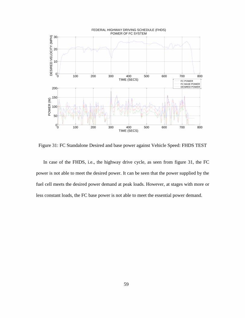
59
Figure 31: FC Standalone Desired and base power against Vehicle Speed: FHDS TEST
In case of the FHDS, i.e., the highway drive cycle, as seen from figure 31, the FC
power is not able to meet the desired power. It can be seen that the power supplied by the
fuel cell meets the desired power demand at peak loads. However, at stages with more or
less constant loads, the FC base power is not able to meet the essential power demand.
0 100 200 300 400 500 600 700 8000
50
100
150
200
TIME (SECS)
PO
WE
R (
W)
0 100 200 300 400 500 600 700 8000
10
20
30
TIME (SECS)
DE
SIR
ED
VE
LO
CIT
Y (
MP
H)
FEDERAL HIGHWAY DRIVING SCHEDULE (FHDS)POWER OF FC SYSTEM
FC POWER
FC BASE POWER
DESIRED POWER

60
Figure 32: FC Standalone Desired and Base Power against Vehicle Speed: US06 TEST
In the US06, as seen from figure 32, the lagging is even more at the peaks. As seen
from the plots, the difference between the desired and supplied power increases with
increase in loads. Highway drive cycle comprises of steady and consistent velocity at
most of the times. The FC was found to be not capable of providing as much power
required in constant speed as well as at times of acceleration.
0 100 200 300 400 500 6000
10
20
30
40
TIME (SECS)
DE
SIR
ED
VE
LO
CIT
Y (
MP
H)
US06POWER OF FC SYSTEM
0 100 200 300 400 500 600-100
0
100
200
300
TIME (SECS)
PO
WE
R (
W)
FC POWER
FC BASE POWER
DESIRED POWER
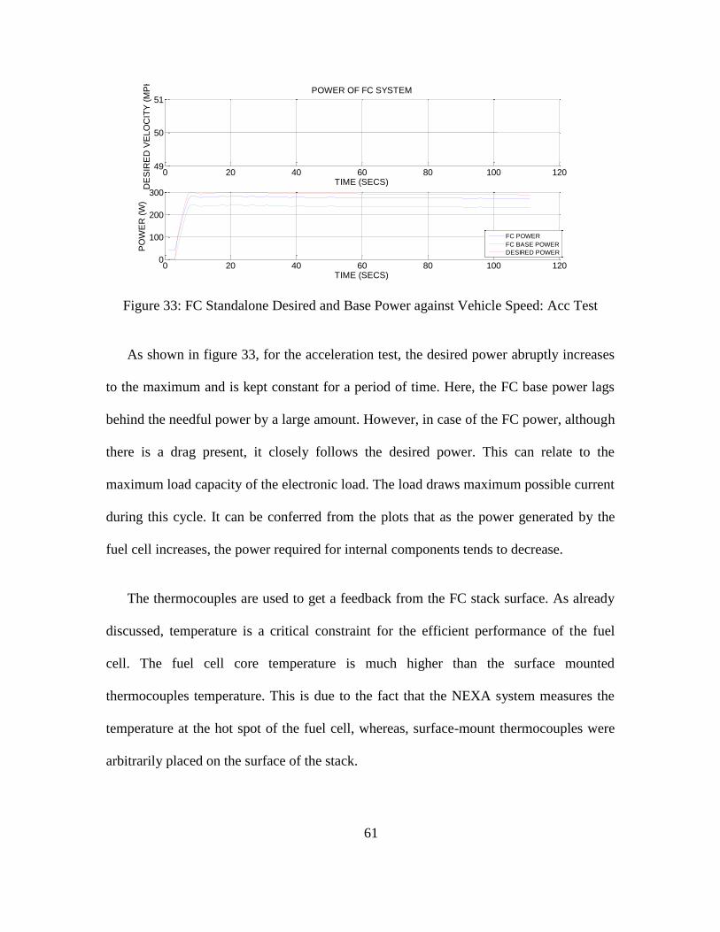
61
Figure 33: FC Standalone Desired and Base Power against Vehicle Speed: Acc Test
As shown in figure 33, for the acceleration test, the desired power abruptly increases
to the maximum and is kept constant for a period of time. Here, the FC base power lags
behind the needful power by a large amount. However, in case of the FC power, although
there is a drag present, it closely follows the desired power. This can relate to the
maximum load capacity of the electronic load. The load draws maximum possible current
during this cycle. It can be conferred from the plots that as the power generated by the
fuel cell increases, the power required for internal components tends to decrease.
The thermocouples are used to get a feedback from the FC stack surface. As already
discussed, temperature is a critical constraint for the efficient performance of the fuel
cell. The fuel cell core temperature is much higher than the surface mounted
thermocouples temperature. This is due to the fact that the NEXA system measures the
temperature at the hot spot of the fuel cell, whereas, surface-mount thermocouples were
arbitrarily placed on the surface of the stack.
0 20 40 60 80 100 12049
50
51
TIME (SECS)
DE
SIR
ED
VE
LO
CIT
Y (
MP
H) ACCELERATION TEST
POWER OF FC SYSTEM
0 20 40 60 80 100 1200
100
200
300
TIME (SECS)
PO
WE
R (
W)
FC POWER
FC BASE POWER
DESIRED POWER
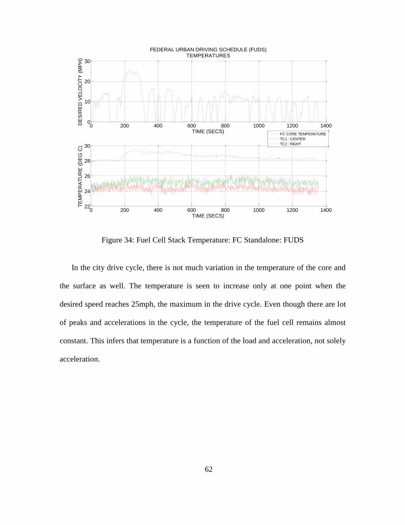
62
Figure 34: Fuel Cell Stack Temperature: FC Standalone: FUDS
In the city drive cycle, there is not much variation in the temperature of the core and
the surface as well. The temperature is seen to increase only at one point when the
desired speed reaches 25mph, the maximum in the drive cycle. Even though there are lot
of peaks and accelerations in the cycle, the temperature of the fuel cell remains almost
constant. This infers that temperature is a function of the load and acceleration, not solely
acceleration.
0 200 400 600 800 1000 1200 14000
10
20
30
TIME (SECS)
DE
SIR
ED
VE
LO
CIT
Y (
MP
H)
FEDERAL URBAN DRIVING SCHEDULE (FUDS)TEMPERATURES
0 200 400 600 800 1000 1200 140022
24
26
28
30
TIME (SECS)
TE
MP
ER
AT
UR
E (
DE
G C
)
FC CORE TEMPERATURE
TC1 : CENTER
TC2 : RIGHT
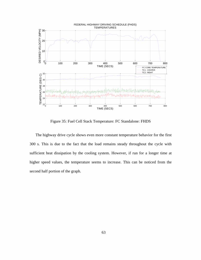
63
Figure 35: Fuel Cell Stack Temperature: FC Standalone: FHDS
The highway drive cycle shows even more constant temperature behavior for the first
300 s. This is due to the fact that the load remains steady throughout the cycle with
sufficient heat dissipation by the cooling system. However, if run for a longer time at
higher speed values, the temperature seems to increase. This can be noticed from the
second half portion of the graph.
0 100 200 300 400 500 600 700 8000
10
20
30
TIME (SECS)
DE
SIR
ED
VE
LO
CIT
Y (
MP
H)
FEDERAL HIGHWAY DRIVING SCHEDULE (FHDS)TEMPERATURES
0 100 200 300 400 500 600 700 80022
24
26
28
30
32
TIME (SECS)
TE
MP
ER
AT
UR
E (
DE
G C
)
FC CORE TEMPERATURE
TC1 : CENTER
TC2 : RIGHT
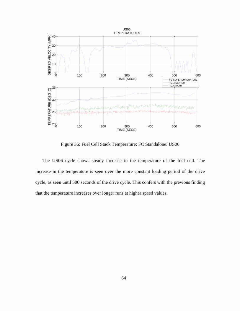
64
Figure 36: Fuel Cell Stack Temperature: FC Standalone: US06
The US06 cycle shows steady increase in the temperature of the fuel cell. The
increase in the temperature is seen over the more constant loading period of the drive
cycle, as seen until 500 seconds of the drive cycle. This confers with the previous finding
that the temperature increases over longer runs at higher speed values.
0 100 200 300 400 500 6000
10
20
30
40
TIME (SECS)
DE
SIR
ED
VE
LO
CIT
Y (
MP
H)
US06 TEMPERATURES
0 100 200 300 400 500 60020
25
30
35
TIME (SECS)
TE
MP
ER
AT
UR
E (
DE
G�C
)
FC CORE TEMPERATURE
TC1 : CENTER
TC2 : RIGHT

65
Figure 37: Fuel Cell Stack Temperature: FC Standalone: Acceleration test
The acceleration test as expected shows an abrupt increase in the temperature of the
FC stack. This cycle consists of constant speed demand of 50 mph throughout the cycle.
The FC core temperature increases from 27.5 to 33⁰C in the time period of 100 seconds.
This increase in temperature is large compared to the shorter time frame. This would
correspond to even larger contrast in full scale FC systems for use in automotive. It is
seen that even if the speed is kept constant at 50 mph, the temperature continues to rise
with almost a constant slope.
0 10 20 30 40 50 60 70 80 90 10049
49.5
50
50.5
51
TIME (SECS)
DE
SIR
ED
VE
LO
CIT
Y (
MP
H)
ACCELERATION TESTTEMPERATURES
0 10 20 30 40 50 60 70 80 90 10020
25
30
35
TIME (SECS)
TE
MP
ER
AT
UR
E (
DE
G�C
)
FC CORE TEMPERATURE
TC1 : CENTER
TC2 : RIGHT
66
Thus, it can be inferred from the above plots that the temperature of the FC stack is a
function of various parameters including, acceleration, power demand, and the length of
run. The impact and relationship between each of these parameters is important to derive
and to understand the temperature distribution and prediction. These relationships can
help to device cooling strategies to incorporate in the full scale automotive FC systems
for their more efficient working. These plots show that not only the overall temperature
but also the temperature distribution in the fuel cell stack is an important consideration.
The center thermocouple temperature remains higher than the side at all times, showing
the temperature at the middle is higher due to less room to dissipate heat. This
temperature distribution can be helpful to modify the geometry of the FC stack and thus
control the maximum temperature.
In the second phase, the hybridization and control strategy implementation of the fuel
cell model takes place. The results of the hybridized fuel cell model are compared to the
fuel cell standalone system. The hybridized fuel cell vehicle model runs on the load
following and the thermostat control strategies.

67
Power Consumption
Figure 38: FC Power Comparison – FC Standalone vs FCHEV: FUDS
As seen from the figure, the power output from the standalone fuel cell are compared
to the power output from the FCHEV in load following and thermostatic control
strategies for the various drive cycle. The green curve represents the FC standalone
power and is seen to be higher than the FCHEV. In case of the thermostatic FCHEV, the
FC power peaks are higher than the load following. This is due to the fact that the
thermostatic strategy is based on the battery SOC and not the power demand, as in the
case of load following.
0 200 400 600 800 1000 1200 14000
1
2
3
4
5
6
7x 10
4 FC Power -- FUDS
Time (Seconds)
Pow
er
(W)
FC Standalone
FC Load Following
FC Thermostatic

68
Figure 39: FC Power Comparison – FC Standalone vs FCHEV: FHDS
Similar trends are seen in case of the FHDS driving cycle. The FC standalone power
represented in red is seen to be higher than the FC load following and FC thermostatic.
The maximum run of the drive cycle is at higher speeds and thus the battery power is
drawn only at peak loads, when the FC is not able to provide the power.
0 100 200 300 400 500 600 700 8000
0.5
1
1.5
2
2.5
3
3.5
4
4.5
5x 10
4 FC -- Power -- FHDS
Time (Seconds)
Pow
er
(W)
FC Standalone
Power Thermostatic
Power Load Following
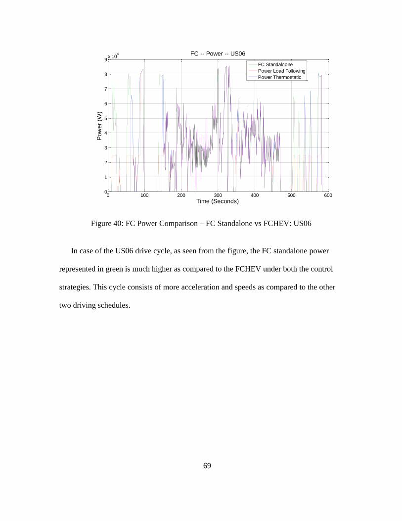
69
Figure 40: FC Power Comparison – FC Standalone vs FCHEV: US06
In case of the US06 drive cycle, as seen from the figure, the FC standalone power
represented in green is much higher as compared to the FCHEV under both the control
strategies. This cycle consists of more acceleration and speeds as compared to the other
two driving schedules.
0 100 200 300 400 500 6000
1
2
3
4
5
6
7
8
9x 10
4 FC -- Power -- US06
Time (Seconds)
Pow
er
(W)
FC Standaloone
Power Load Following
Power Thermostatic
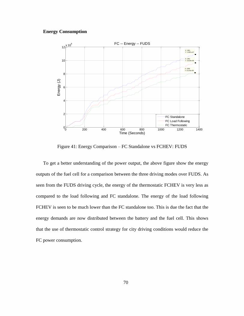
70
Energy Consumption
Figure 41: Energy Comparison – FC Standalone vs FCHEV: FUDS
To get a better understanding of the power output, the above figure show the energy
outputs of the fuel cell for a comparison between the three driving modes over FUDS. As
seen from the FUDS driving cycle, the energy of the thermostatic FCHEV is very less as
compared to the load following and FC standalone. The energy of the load following
FCHEV is seen to be much lower than the FC standalone too. This is due the fact that the
energy demands are now distributed between the battery and the fuel cell. This shows
that the use of thermostatic control strategy for city driving conditions would reduce the
FC power consumption.
0 200 400 600 800 1000 1200 14000
2
4
6
8
10
12x 10
6
X: 1358
Y: 8.143e+06
FC -- Energy -- FUDS
Time (Seconds)
Energ
y (
J)
X: 1361
Y: 1.087e+07
X: 1361
Y: 9.624e+06
FC Standalone
FC Load Following
FC Thermostatic

71
In case of the FHDS driving cycle (Refer to Appendix B), the difference between the
FC energy of three driving modes is seen to be not much. Although the trends of FC
standalone energy being highest and the thermostatic being lower than the load following
are in consistence with the FUDS drive cycle, the difference is less. This is because in the
highway drive cycle, the power demands remain more or less constant and there is very
less braking. In the same line, there are seen to similar trends in case of the US06 drive
cycle (Appendix B). However, the difference between the energies is huge, even more
than the FUDS drive cycle.
H2 Consumption
Figure 42: H2 Consumption Comparison – FC Standalone vs FCHEV: FUDS
0 200 400 600 800 1000 1200 14000
0.05
0.1
0.15
0.2
0.25
X: 1361
Y: 0.1622
FC H2 Consumption -- FUDS
Time (Seconds)
H2 C
onsum
ption (
KG
)
X: 1360
Y: 0.2072
X: 1361
Y: 0.1843
FC Standalone
FCHEV - Load Following
FCHEV - Thermostatic

72
The figure shows the hydrogen fuel consumption in case of the standalone fuel cell
system and the Hybrid fuel cell running in the load following and thermostatic modes
over the FUDS driving cycle. In case of the FUDS drive cycle, the hydrogen fuel
consumption of FC standalone is recorded to be 0.2072 kg. Whereas, the same for load
following and thermostatic are 0.0.1863 kg and 0.1622 kg respectively. The following
table summarizes the findings over the three driving cycles relating to the hydrogen fuel
consumption. Please refer to Appendix C for the graphs of FHDS and US06.
FC Standalone H2
Consumption (kg)
FCHEV Load
Following H2
Consumption (kg)
FCHEV
Thermostatic H2
Consumption (kg)
FUDS 0.2072 0.1843 0.1622
FHDS 0.2583 0.2470 0.2382
US06 0.3590 0.2913 0.2800
Table 6: H2 Consumption Comparison
There is seen to be an 11.5% decrease in case of load following and almost 12% more
decrease in case of the thermostatic control strategy.
In case of the FHDS driving cycle (Appendix C), the decrease in hydrogen
consumption in load following mode is 4% and in the thermostatic mode is even 8.8%
less. Although there was less difference in the power of these two strategies in this drive
cycle, the hydrogen consumption has drastically reduced as the efficiency of the fuel cell
has been increased. This was due to the fact that the operating region of the fuel cell has
changed. With the implementation of control strategies, the fuel cell is now running at a
more efficient region than the standalone system.
73
In case of the US06 drive cycle (Appendix C), the hydrogen consumption of the load
following mode running fuel cell decreases by almost 20%. This difference is huge and
very drastic. However, less difference is noticed in the hydrogen consumption of the
thermostatic and load following FCHEV’s. The results are in accordance with the
aggressive accelerations present in the US06.
Comparison With Honda FCX Clarity
HONDA FCX CLARITY SPECIFICATIONS
100kW PEMFC
Li-ion Battery wit output of 288 V
134 HP Electric Motor
Fuel economy (City): 58 miles/kg of H2*
Fuel economy (Highway): 60 miles/kg of H2*
(*Data obtained from US Department of Energy
http://www.fueleconomy.gov/feg/fcv_sbs.shtml)
The following table shows a comparison of hydrogen fuel consumptions between the
simulated FCHEV and a real world FCV,i.e., Honda FCX Clarity. The hydrogen
consumption are converted to fuel economy in miles per kg of hydrogen for better
understanding.

74
Fuel Economy
(miles/kg of H2)
Honda FCX Clarity FCHEV Load
Following
FCHEV
City 58 41 46
Highway 60 40 44
Table 7: Fuel Economy Comparison: Honda FCX Clarity Vs Modelled Fuel Cell Vehicle
The difference in fuel economies of the simulated and real world FCV can be due to a
number of factors including:
The power of the fuel cell modelled system is 80 kW, as compared to the 100kW of
Honda FCX Clarity.
The type of drive cycles assumed in the modeling do not 100% represent the real
world road load conditions.
The type of energy management strategy used in Honda FCX unknown.
The comparison of fuel economy of Honda FCX gives a realistic base to verify the
modelled FCV. It is also clear from the results that the efficiency of the energy
management control strategy plays a vital role in the performance of the hybrid vehicle.
Thus it can be inferred from the above results that the successful HiL implementation
of the control strategies in FCHEV was achieved. The results also show that significant
improvements can be achieved by the use of logically developed energy management
strategies. The behavior of the fuel cell under these control strategies has been verified by
the real HiL testing. The results show that the overall hydrogen fuel consumption of the
75
thermostatic control strategy is lower than the load following control strategies. This
deduction is in accordance to the simulation results of many experiments done. The
results also shed light on the dynamic behavior of the fuel cell under different control
strategies. The HiL testing showed the actual hydrogen consumption and the power
response of the 1.2 kW fuel cell. The response of the fuel cell under FCHEV is more
dynamic and up to the requirements than just the standalone fuel cell.
Closed-loop testing thus can prove to be a great tool in early design testing and
modification of hybrid energy systems. Today’s automotive scenario requires vehicles
with ability to supply more power demands as well as being able to consistent with
abrupt changes due to increasing urban traffic. For fuel cell vehicles to cope with the
requirements and replace IC engines, design changes is the need of the hour. Closely
following the relation between the parameters discussed and developing test stands that
are more efficient can help to achieve this goal.
Limitations Associated
Throughout the project there have been realistic assumptions made relating to the
specification of different hardware components modelled. These assumptions, although
referring to the real world component data, might not be very accurate. Thus, they pose as
limitations as well.
Since the development of the NEXA 1.2 fuel cell, used in the HiL implementation of
this project, there have been many advances in the design and working of PEM fuel cells.
Thus the results obtained from the NEXA 1.2 fuel cell would be less efficient compared
to the more efficient fuel cell systems used currently.

76
Also, the hydrogen consumption in the modelled fuel cell system is assumed to be
100% efficient, which is not the case in the real fuel cell. There are some loses that need
to be taken into account for more realistic results. For the scope of the project and limited
availability of resources, these assumptions have been made to get the best possible
results.
77
7: CONCLUSIONS AND FUTURE SCOPE OF WORK
Closed Loop Feedback Fuel Cell Hardware in-the-Loop (FCHIL) was implemented
successfully and the performance of the 1.2 Nexa fuel cell was evaluated under various
standard and custom specific driving schedules. The power requirement and the thermal
performance of the fuel cell stack were monitored over wide range of load scenarios.
It was found that the standalone FC was capable of providing non-uniform power
consistently as required by the city driving schedule. However, at points with more or
less constant loads, the FC base power lagged behind essential power demand by some
amount. As seen from the plots, the difference between the desired and supplied power
increases with increase in loads. The standalone FC was not able to provide as much
power required in constant speed as well as at times of high acceleration. It has been
noticed that fuel cell stack temperature is a function of the load and acceleration, not
solely acceleration. If run for a long time, the temperature is seen to increase.
In case of the FCHEV regardless of the control strategies, it was noticed that the FC
was able to provide power for all the drive cycles. The transient response of the FC as
compared to the standalone system was more. This shows that the use of control
strategies can definitely enhance the performance of the fuel cell and decrease the
hydrogen consumption significantly.
Furthermore, to this research, different control strategies for the optimum working of
the fuel cell can be developed and tested on the closed loop HiL test bench. Control
strategies based on the future driving conditions such as the pattern recognition and

78
terrain preview could even more optimize the working of the FCHEV. These strategies
review the past power demands over a specific period of time and make decisions on the
fuel cell on/off state. This would allow the fuel to run in the maximum efficiency region,
thus decreasing the hydrogen consumption. In the future research, such energy
management strategies could be tested on the fuel cell test bench to study the real fuel
cell behavior.

79
REFERENCES
1. Guenter Randolf, Robert M. Moore, Test system design for Hardware-in-Loop
evaluation of PEM fuel cells and auxiliaries, Journal of Power Sources, Volume 158,
Issue 1, 14 July 2006, Pages 392-396, ISSN 0378-7753,
(http://www.sciencedirect.com/science/article/pii/S0378775305013790)
2. Zijad Lemeš, Andreas Vath, Th. Hartkopf, H. Mäncher, Dynamic fuel cell models
and their application in hardware in the loop simulation, Journal of Power Sources,
Volume 154, Issue 2, 21 March 2006, Pages 386-393, ISSN 0378-7753,
(http://www.sciencedirect.com/science/article/pii/S0378775305014308)
3. R.M. Moore, K.H. Hauer, G. Randolf, M. Virji, Fuel cell hardware-in-loop, Journal
of Power Sources, Volume 162, Issue 1, 8 November 2006, Pages 302-308, ISSN
0378-7753, 10.1016/j.jpowsour.2006.06.066.
4. Hoogers, Gregor. 2003. Fuel cell technology handbook. Boca Raton, Fla: CRC Press.
5. Guenter Randolf, Robert M. Moore, Test system design for Hardware-in-Loop
evaluation of PEM fuel cells and auxiliaries, Journal of Power Sources, Volume 158,
Issue 1, 14 July 2006, Pages 392-396, ISSN 0378-7753,
10.1016/j.jpowsour.2005.09.058.
6. Heywood, John B. 1988. Internal combustion engine fundamentals. New York:
McGraw-Hill.
7. Barbir, Frano (2013). PEM Fuel Cells - Theory and Practice. Elsevier
8. Wu, Jifeng. 2013. PEM Fuel Cell Testing and Diagnosis. Burlington: Elsevier
Science, 2013. eBook Collection (EBSCOhost), EBSCOhost (accessed June 11,
2014).
9. Stobart, Richard. 2001. Fuel cell technology for vehicles. Warrendale, PA: Society of
Automotive Engineers.

80
10. Fuel cell vehicles. 2013. PR Newswire, May 27, 2013.
http://login.ezproxy1.lib.asu.edu/login?url=http://search.proquest.com/docview/1355
506278?accountid=4485 (accessed June 11, 2014).
11. S.G. Chalk, J.F. Miller, J. Power Sources 159 (2006) 73–80.
12. A. Burke, Presentation at ARB ZEV Technology Symposium, Sacramento,
California, September 27, 2006, http://www.arb.ca.gov/msprog/zevprog/
symposium/presentations/burke1.pdf.
13. Rittmar von Helmolt, Ulrich Eberle, Fuel cell vehicles: Status 2007, Journal of Power
Sources, Volume 165, Issue 2, 20 March 2007, Pages 833-843, ISSN 0378-7753,
http://dx.doi.org/10.1016/j.jpowsour.2006.12.073.
14. Society of Automotive Engineers, and Powertrain & Fluid Systems Conference and
Exhibition. 2004. Hybrid electric vehicle technology. Warrendale, PA: Society of
Automotive Engineers.
15. ECMT (2001), Vehicle Emission Reductions, OECD Publishing.
doi: 10.1787/9789264193642-en 16 1966 GM electrovan smithsonian collection
correction. 2010. Hydrogen Cars Now [Hydrogen Cars Now - BLOG] (Aug 05),
http://login.ezproxy1.lib.asu.edu/login?url=http://search.proquest.com/docview/7370
83820?accountid=4485 (accessed June 11, 2014).
16. 1966 GM electrovan smithsonian collection correction. 2010. Hydrogen Cars Now
[Hydrogen Cars Now - BLOG] (Aug 05),
http://login.ezproxy1.lib.asu.edu/login?url=http://search.proquest.com/docview/7370
83820?accountid=4485 (accessed June 11, 2014).
17. Fuel Cell Vehicles. (2012, Fleet Maintenance, 16, 24-27. Retrieved from
http://login.ezproxy1.lib.asu.edu/login?url=http://search.proquest.com/docview/1114
878366?accountid=4485
81
18. Peter, John. 2003. GM Hydrogen3. Automotive Industries 183, (1) (01): 21,
http://login.ezproxy1.lib.asu.edu/login?url=http://search.proquest.com/docview/2360
04209?accountid=4485 (accessed June 11, 2014).
19. Hyun Tae Hwang, Arvind Varma, Hydrogen storage for fuel cell vehicles, Current
Opinion in Chemical Engineering, Volume 5, August 2014, Pages 42-48, ISSN 2211-
3398 (http://www.sciencedirect.com/science/article/pii/S2211339814000446)
20. Real-time and Power Hardware-in-the-loop Simulation of PEM Fuel Cell Stack
System By Jung, JH, Journal of Power Electronics, 03/201, ISSN: 1598-2092,
Copyright (c) 2011 Institute for Scientific Information.
21. Xi Li, Zhong-Hua Deng, Dong Wei, Chun-Shan Xu, Guang-Yi Cao, Novel variable
structure control for the temperature of PEM fuel cell stack based on the dynamic
thermal affine model, Energy Conversion and Management, Volume 52, Issue 11,
October2011, Pages 3265-3274, ISSN 0196-8904,
10.1016/j.enconman.2011.05.013.Y
22. Dynamic modelling and hardware-in-the-loop testing of PEMFC Andreas Vath ,
Zijad Lem˘es b, Hubert M¨ancher b, Matthias S¨ohn a, Norbert Nicoloso a, Thomas
23. Gauchia, L.; Sanz, J., "A Per-Unit Hardware-in-the-Loop Simulation of a Fuel
Cell/Battery Hybrid Energy System," Industrial Electronics, IEEE Transactions on ,
vol.57, no.4, pp.1186,1194, April 2010
24. Rajesh K. Ahluwalia, X. Wang, A. Rousseau Argonne National Laboratory, 9700
South Cass Avenue, Argonne, IL 60439, USA.
25. Energy management strategy for fuel cell/battery/ultracapacitor hybrid vehicle based
on fuzzy logic Qi Li , Weirong Chen , Yankun Li , Shukui Liu , Jin Huang a a School
82
of Electrical Engineering, Southwest Jiaotong University, Chengdu 610031, Sichuan
Province, China b Chengdu Electric Power Bureau, Chengdu 610021, Sichuan
Province, China
26. IEEE TRANSACTIONS ON INTELLIGENT TRANSPORTATION SYSTEMS,
VOL. 13, NO. 4, DECEMBER 2012 Energy Management for Fuel-Cell Hybrid
Vehicles Based on Specific Fuel Consumption Due to Load Shifting ˙Ismail Levent
Sarıoˇglu, Olaf P. Klein, Hendrik Schröder, and Ferit Küçükay
27. MathWorks Inc. http://ctms.engin.umich.edu/CTMS/index.php?aux=Basics_Simulink
28. Environmental Protection Agency.
http://www.epa.gov/nvfel/testing/dynamometer.htm
29. K. Rajashekara, Fuel Cell Technology for Vehicles (2000) 179–187. [4] K. Jeong, B.
Oh, Journal of Power Sources 1005 (2002) 58–65
30. R.K. Ahluwalia, X. Wang, A. Rousseau, R. Kumar, Fuel economy of hydrogen fuel
cell vehicles, J. Power Sources 130 (2003) 192–201.
31. Plug-in Hybrid Electric Vehicle Supervisory Control Strategy Considerations for
Engine Exhaust Emissions and Fuel Use Patrick M. Walsh Thesis submitted to the
faculty of the Virginia Polytechnic Institute and State University in partial fulfillment
of the requirements for the degree of Master of Science In Mechanical Engineering
Douglas J. Nelson Mehdi Ahmadian Alan Kornhauser May 4, 2011 Blacksburg, VA
32. Jianping Gao; Fengchun Sun; Hongwen He; Zhu, G.G.; Strangas, E.G., "A
Comparative Study of Supervisory Control Strategies for a Series Hybrid Electric
Vehicle," Power and Energy Engineering Conference, 2009. APPEEC 2009. Asia-
Pacific , vol., no., pp.1,7, 27-31 March 2009 doi: 10.1109/APPEEC.2009.4918038

83
33. Jazar, Reza N. 2014. Vehicle dynamics: theory and application.
http://dx.doi.org/10.1007/978-1-4614-8544-5.

84
APPENDIX A
ELECTRIC MOTOR AND BATTERY SPECIFICATIONS

85
Electric Motor Specifications
o Power Output: 80kW
o Horsepower: 107.28
Battery Specifications
o Lithium Ion Battery
o Output (Volts): 274 V
o Power Capacity: 30kW
o Battery Capacity: 110 Ah

86
APPENDIX B
ENERGY CONSUMPTION RESULTS: FHDS & US06

87
Figure 43: Energy Comparison– FC Standalone vs FCHEV: FHDS
Figure 44: Energy Comparison– FC Standalone vs FCHEV: US06
0 100 200 300 400 500 600 700 8000
5
10
15x 10
6
X: 772
Y: 1.353e+07
Time (Seconds)
FC Energy -- FHDS
En
erg
y (
J)
X: 772
Y: 1.446e+07X: 772
Y: 1.389e+07
FC Standalone
FCHEV Thermostatic
FC Load Following
0 100 200 300 400 500 6000
2
4
6
8
10
12
14
16
18x 10
6
X: 601
Y: 1.385e+07
FC -- Energy -- US06
Time (Seconds)
En
erg
y (
J)
X: 600
Y: 1.44e+07
X: 601
Y: 1.709e+07
Energy Load Following
Energy Thermostatic
Energy Standalone

88
APPENDIX C
H2 CONSUMPTION RESULTS: FHDS &US06
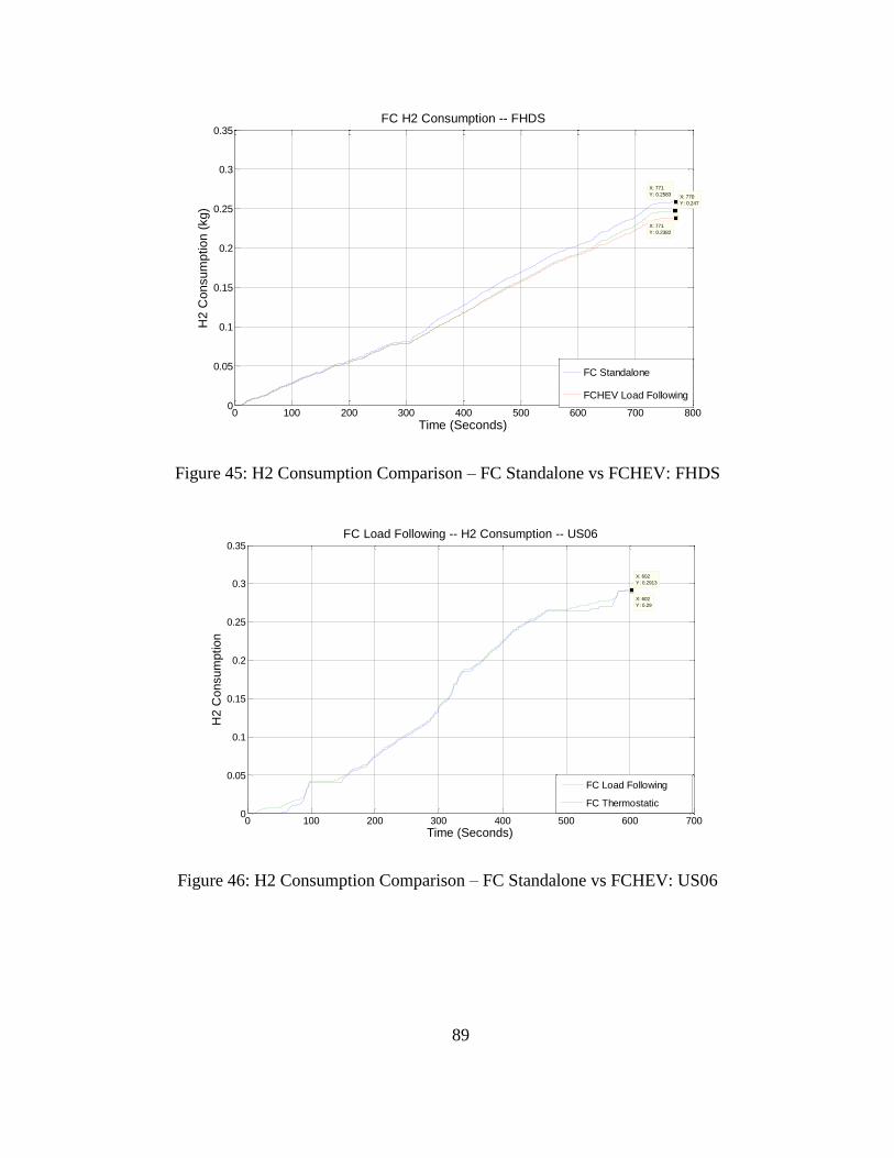
89
Figure 45: H2 Consumption Comparison – FC Standalone vs FCHEV: FHDS
Figure 46: H2 Consumption Comparison – FC Standalone vs FCHEV: US06
0 100 200 300 400 500 600 700 8000
0.05
0.1
0.15
0.2
0.25
0.3
0.35
X: 770
Y: 0.247
FC H2 Consumption -- FHDS
Time (Seconds)
H2 C
onsum
ption (
kg)
X: 771
Y: 0.2382
X: 771
Y: 0.2583
FC Standalone
FCHEV Load Following
0 100 200 300 400 500 600 7000
0.05
0.1
0.15
0.2
0.25
0.3
0.35
X: 602
Y: 0.29
Time (Seconds)
H2 C
onsum
ption
FC Load Following -- H2 Consumption -- US06
X: 602
Y: 0.2913
FC Load Following
FC Thermostatic