Embed Size (px)
Citation preview

Model-based analysis of respiratory mechanicsfor diagnosis of cardiopulmonary diseases
Von der Fakultät für Elektrotechnik und Informationstechnik derRheinisch-Westfälischen Technischen Hochschule Aachen zur Erlangung desakademischen Grades eines Doktors der Ingenieurwissenschaften genehmigte
Dissertation
vorgelegt von
Diplom-IngenieurHoang Chuong Ngo Nguyen
aus Ho Chi Minh City, Vietnam
Berichter: 1) Univ.-Prof. Dr.-Ing. Dr. med. Steffen Leonhardt, Aachen2) Assistant Prof. Dr.Ir. F.H.C. de Jongh, Twente3) Prof. Dr. med. Klaus Tenbrock, Aachen
Tag der mündlichen Prüfung: 18.01.2019
Diese Dissertation ist auf den Internetseiten der Universitätsbibliothekonline verfügbar.


Acknowledgment
This dissertation was conducted during my work as a research assistant at theChair of Medical Information Technology (MedIT), Helmholtz Institute forBiomedical Engineering at RWTH Aachen between 2013 and 2018. I wouldlike to express my sincere gratitude to my doctor father, Professor SteffenLeonhardt, the holder of the Chair for Medical Information Technology, forthe great opportunity to carry out such an interesting research. His scien-tific competence and ambition have constantly guided and encouraged me forthe competition of this thesis. His willingness to give his time so generouslyhas been very much appreciated. I also thank Professor Frans de Jongh andProfessor Klaus Tenbrock for serving as co-examiner, as well as Professor GerdAscheid and Professor Albert Moser for serving on the examination committee.Furthermore, I would also like to thank to my group leader, Dr. Berno
Misgeld for his advice and assistance in keeping my progress on schedule. Ialso would like to express my very great appreciation to Dr. Lehman for heradvice and her help in acquisition and analysis of the EIT data.My gratitude is specifically given to Philips Research for the financial support
during my whole dissertation period. My grateful thanks are also extended toMr. Thomas Vollmer and Mr. Stefan Winter from Philips for their useful andconstructive recommendations on this work.I wish to thank various students for their contribution to this thesis: Stephan
Dahlmanns, Carlos Munoz, Falk Dippel, Philip Ackermann, Sarah Spagnesi,Karl Krüger, Alexander Kube, Rober Schlözer, Ai Bahram, and Tony Zhang.I also thank my former and current colleagues Stephan Dahlmanns, Philip vonPlaten, Markus Lüken, Bernhard Penzlin, Christian Brendle, Christoph Weiss,Daniel Rüschen, and others for the great time at MedIT.In addition, I would like to extend my thanks to all my proof-readers and
further friends and colleagues who were involved in the correction process ofthe thesis.Finally, I wish to thank my parents and my sister for their unconditional
love, consistent care, support and encouragement throughout my study andphD time.
v


Contents
Acknowledgment v
1 Introduction 11.1 Motivation . . . . . . . . . . . . . . . . . . . . . . . . . . . . . 1
1.1.1 Obstructive pulmonary diseases . . . . . . . . . . . . . . 11.1.2 Restrictive pulmonary diseases . . . . . . . . . . . . . . 2
1.2 History of respiratory researches . . . . . . . . . . . . . . . . . 31.3 Methodology of mathematical modeling of biomedical systems . 5
1.3.1 Forward modeling . . . . . . . . . . . . . . . . . . . . . 51.3.2 Inverse modeling . . . . . . . . . . . . . . . . . . . . . . 6
1.4 Objectives of the research . . . . . . . . . . . . . . . . . . . . . 71.5 Organization of this book . . . . . . . . . . . . . . . . . . . . . 8
2 Fundamentals 92.1 Physiological background . . . . . . . . . . . . . . . . . . . . . 9
2.1.1 Physiology of the respiratory tract . . . . . . . . . . . . 92.1.2 Respiratory mechanics . . . . . . . . . . . . . . . . . . . 132.1.3 Physiology of heart, circulation, and lymphatics . . . . 16
2.2 Pulmonary function diagnostics . . . . . . . . . . . . . . . . . . 202.2.1 Spirometry . . . . . . . . . . . . . . . . . . . . . . . . . 222.2.2 Helium dilution and nitrogen washout methods . . . . . 242.2.3 Body plethysmography . . . . . . . . . . . . . . . . . . . 242.2.4 Rapid interrupter technique . . . . . . . . . . . . . . . . 262.2.5 Esophageal catheter . . . . . . . . . . . . . . . . . . . . 272.2.6 Forced Oscillation Technique . . . . . . . . . . . . . . . 28
2.3 Mechanical ventilation . . . . . . . . . . . . . . . . . . . . . . . 302.3.1 Continuous positive airway pressure (CPAP) . . . . . . 302.3.2 Pressure- and volume-controlled ventilation . . . . . . . 30
2.4 Electrical Impedance Tomography . . . . . . . . . . . . . . . . 312.5 Object-oriented modeling language for biophysical modeling . . 33
3 Respiratory modeling 373.1 Non-linear model components . . . . . . . . . . . . . . . . . . . 37
3.1.1 Airways and airspaces . . . . . . . . . . . . . . . . . . . 373.1.2 Tissue and chest wall . . . . . . . . . . . . . . . . . . . 45
3.2 The two-degree-of-freedom model . . . . . . . . . . . . . . . . . 493.2.1 Parametrization and implementation . . . . . . . . . . . 50
vii

Contents
3.2.2 Simulation results . . . . . . . . . . . . . . . . . . . . . 523.2.3 The linearized respiratory model . . . . . . . . . . . . . 54
3.3 Model-based analysis of the interrupter technique . . . . . . . . 573.3.1 Model behavior during an interruption . . . . . . . . . . 583.3.2 Simulation-based analysis of the interrupter technique . 593.3.3 Pendelluft and the Otis parallel model structure . . . . 63
3.4 Summary . . . . . . . . . . . . . . . . . . . . . . . . . . . . . . 64
4 Model-based parameter estimation with the forced oscillation tech-nique (FOT) 674.1 Measurement of respiratory impedance . . . . . . . . . . . . . . 674.2 Modeling and parameter identification . . . . . . . . . . . . . . 70
4.2.1 A survey of lung models used in Forced Oscillation Tech-nique . . . . . . . . . . . . . . . . . . . . . . . . . . . . 70
4.2.2 Model-based analysis . . . . . . . . . . . . . . . . . . . . 724.2.3 Model hierarchy and recommendations . . . . . . . . . . 77
4.3 The volume-dependent FOT . . . . . . . . . . . . . . . . . . . . 794.3.1 Principles of the volume-dependent FOT . . . . . . . . 794.3.2 The reduced non-linear model . . . . . . . . . . . . . . . 804.3.3 Results of the parameter estimation . . . . . . . . . . . 83
4.4 The nasal FOT . . . . . . . . . . . . . . . . . . . . . . . . . . . 854.5 Summary . . . . . . . . . . . . . . . . . . . . . . . . . . . . . . 89
5 Modeling of cardiopulmonary interactions and cardiogenic congestion 915.1 Modeling of heart and circulation . . . . . . . . . . . . . . . . . 91
5.1.1 Atria, ventricles and heart valves . . . . . . . . . . . . . 915.1.2 Septum and pericardium . . . . . . . . . . . . . . . . . . 935.1.3 Vascular arteries and veins . . . . . . . . . . . . . . . . 945.1.4 Baseline simulation of the cardiovascular system . . . . 96
5.2 Cardiopulmonary hemodynamic interactions . . . . . . . . . . . 995.2.1 Simulation results . . . . . . . . . . . . . . . . . . . . . 100
5.3 The fluid balance and the lymphatic system . . . . . . . . . . . 1065.3.1 Model development . . . . . . . . . . . . . . . . . . . . . 1065.3.2 Model extension for cardiogenic pulmonary congestion . 112
5.4 Simulation results . . . . . . . . . . . . . . . . . . . . . . . . . 1165.4.1 Fluid filtration through the capillary walls . . . . . . . . 1165.4.2 Lymphatic absorption . . . . . . . . . . . . . . . . . . . 1185.4.3 Cardiogenic pulmonary congestion and CPAP treatment 118
5.5 Discussion and summary . . . . . . . . . . . . . . . . . . . . . . 122
viii
Contents
6 Assessment of global and regional ventilation using EIT 1236.1 Diagnosis of pulmonary function with EIT during forced expi-
ratory maneuvers . . . . . . . . . . . . . . . . . . . . . . . . . . 1246.1.1 Study design . . . . . . . . . . . . . . . . . . . . . . . . 1246.1.2 Linearity between EIT and spirometry in healthy adults 1276.1.3 Linearity between EIT and spirometry in pediatric pa-
tients with asthma . . . . . . . . . . . . . . . . . . . . . 1286.1.4 Regional EIT-derived flow volume (FV) loop . . . . . . 133
6.2 Introduction of oscillatory Electrical Impedance Tomography(oEIT) . . . . . . . . . . . . . . . . . . . . . . . . . . . . . . . . 1376.2.1 Visibility of FOT frequencies in EIT signal . . . . . . . 1376.2.2 The band-pass filtered oEIT signal . . . . . . . . . . . . 138
6.3 Summary . . . . . . . . . . . . . . . . . . . . . . . . . . . . . . 141
7 Discussion and outlook 143
A Appendix 147
B Publications 159
Bibliography 163
ix

Contents
Abbreviation
Symbol Meaning
ARDS Acute respiratory distress syndromeASB Assisted spontaneous breathingATS American Thoracic SocietyBiPAP Bilevel positive airway pressureBSL BronchospasmolysisCHF Congestive heart failureCOPD Chronic obstructive diseaseCPAP Continuous positive airway pressureCPS Cardiopulmonary systemCVS Cardiovascular systemECG ElectrocardiogramEDPVR End-diastole pressure-volume relationshipEIT Electrical impedance tomographyERS European Respiratory SocietyESPVR End-systole pressure-volume relationshipFEV05 Forced expiratory volume in 0.5 secondFEV1 Forced expiratory volume in 1 secondFOT Forced oscillation techniqueFRC Functional residual capacityFV Flow-volumeFVC Forced vital capacityGOLD Global Initiative for Chronic Obstructive Lung DiseaseIGV Intra-thoracic gas volumeITBV Intra-thoracic blood volumeLV Left ventricleMEF25 Maximum expiratory flow at 25% of FVCMEF50 Maximum expiratory flow at 50% of FVCMEF75 Maximum expiratory flow at 75% of FVCMRI Magnet resonance imagingODE Ordinary differential equationoEIT Oscillatory electrical impedance tomographyOOML Object-oriented modeling languageOSA Obstructive sleep apneaPCV Pressure-controlled ventilationPCW Pulmonary capillary wedge (pressure)n
x

Contents
Symbol Meaning
PEEP Positive end-expiratory pressurePEF Peak expiratory flowPFT Pulmonary function testPIP Positive inspiratory pressurePV Pressure-volumeRLD Restrictive pulmonary diseaseRV Right ventricleSD Standard deviationSV Stroke volumeTI Tiffeneau indexTLC Total lung capacityTOP Threshold opening pressureTPR Total peripheral resistance (circulation)VC Vital capacityVCV Volume-controlled ventilationVT Tidal volumeWHO World Health OrganizationWOB Work of breathing
xi

Contents
Physical parameters
Symbol Meaning Unit
p,P Pressure cmH2O,mmHgt Time sV Volumen L
V Flow L/sR Resistance cmH2O/L/sC Compliance L/cmH2OI Inertance cmH2O/L/s2
f Frequency HzZ Impedance cmH2O/L/sG Conductance L/(cmH2Os)sG Specific conductance 1/(cmH2Os)sR Specific resistance cmH2Osτ Time constant sϕ Phase radianG Tissue damping (constant-phase) undefinedH Tissue elastance (constant-phase) undefinedZR Resistive impedance cmH2O/L/sZR Reactive impedance cmH2O/L/s
xii

Contents
Indexes
Symbol Meaninga, art arterialalv alveolarao airway openingao aortic (circulation)av aortic valveaw airwayb bronchialc centralc+cw central and chest wallcap capillarycw chest walled diastolices systolices esophagealf filtrationint interrupter (for resistance)int interstitialL lungla left atrialle left (lung)leak leakageliq liquidlrs lower respiratory systemlv left ventricularlym lymphaticmeas measuredmus respiratory musclesnaw nasal airwayos oscillation, oscillatoryosm osmoticp peripheralpa pulmonary arterialPE pleural extendedpl pleuralpul pulmonary
xiii

Contents
IndexesSymbol Meaningpv pulmonary venouspvc pulmonary venous capillaryra right atrialres,R resistiveri right (lung)rs respiratoryrv right ventricularsa systemic arterialsafe safety factorstat staticsys systemictc tricuspid valveti tissuetr transmuralv,ven venousvc vena cavaX reactive
xiv

1 Introduction
Breathing in, there is only the present moment.Breathing out, it is a wonderful moment.
Thich Nhat Hanh
1.1 Motivation
Breathing is fundamental for the survival of living beings by delivering oxy-gen and removing carbon dioxide. Disturbances caused by diseases or injuriescan lead to serious physiological damages. Respiratory failures in humans areclassified into obstructive and restrictive pulmonary diseases.
1.1.1 Obstructive pulmonary diseases
People with obstructive pulmonary disease often face shortness of breath. Anobstruction, flow limitation, or air "trapped" inside the lungs occurs if an ab-normally high amount of air remains in the lungs at the end of a full exhalation.The obstruction becomes worse during activity or exertion, when the rate ofbreathing is higher than normal. The main reason for obstruction is damage ornarrowing of the airways. Common obstructive pulmonary diseases are chronicobstructive pulmonary disease (COPD), asthma, sleep apnea, bronchiectasis,and cystic fibrosis.COPD is the most common obstructive pulmonary disease. According to
the World Health Organization (WHO) and the Global Initiative for ChronicObstructive Lung Disease, COPD is the cause of about 3 million deaths peryear (2015) and will rank third in the causes of death in 2020 [25,211]. COPD’ssymptoms are coughing and secretion that are usually associated with chronicbronchitis and pulmonary emphysema [139]. Main causes of airway obstructionare air contaminants (for example, cigarette smoke or fine dust) that are locatedin the lungs and trigger inflammatory processes. COPD worsens with aging.Lifelong smokers have a 50% probability of developing COPD developed duringtheir lifetime [106].Asthma (or bronchial asthma) is the most common chronic disease among
children. It is a chronic, incurable disease caused by hypersensitivity, e.g. byallergies, which leads to a long-term inflammation and narrowing of the air-ways. Typical symptoms are wheezing, coughing, shortness of breath, andincreased work of breathing (WOB). While the WHO estimates 334 millionpeople worldwide to suffer from asthma [1, 141], the International Study ofAsthma and Allergies in Childhood reported that about 14% of the world’s
1

1 Introduction
children are likely to have asthmatic symptoms (2014). Since uncontrolledasthma can damage the airways permanently, it’s crucial to get asthma diag-nosed and receive treatment as soon as possible.The common diagnostic tool for COPD and asthma is spirometry [1, 211].
Spirometry is a non-invasive pulmonary function test (PFT) which is helpful inassessing breathing patterns in the form of flow-volume (FV) loops that iden-tify abnormal conditions. Results of spirometry tests are volume parameters,such as forced vital capacity (FVC), or forced expiratory volume in one sec-ond (FEV1). These indicies are indirect parameters, which means they do notprovide physical characteristics of lung mechanics such as resistance or com-pliance, but rather give an indicator for the exhaling time and the related flowlimitation. Other pulmonary function tools such as whole-body plethysmogra-phy, interruption technique, or oscillometry, which measure directly mechanicalparameters of the lungs, have proven their discriminative power in assessinglung mechanics in clinical studies. However, they are not listed as standardizedPFTs in assessing COPD and asthma.Also, there are several limitations in standard spirometry. First, it requires
strong patients’ cooperation during the forced expiration maneuver, hence, isnot suited for infants, young children, sleeping patients, or patients with severediseases. Second, spirometry and other PFTs are limited to global function ofthe lungs, while regional information can be beneficial to assess heterogeneouschanges in diseased lungs and to improve treatment. Both aspects will bediscussed later in this work.
1.1.2 Restrictive pulmonary diseasesRestrictive pulmonary diseases (RLDs) are conditions in which the lungs cannotbe fully filled with air. It is defined as a reduction of total lung capacity (TLC)below the 5th percentile of the predicted value, while the ratio FEV1/FCV ispreserved [181]. Restrictive diseases are often caused by an increased stiffnessin the lungs, with the restricted area in the lung parenchyma, in the pleu-ral space, or in the chest wall. Interstitial lung diseases, sarcoidosis, cardio-genic congestion and edema, acute lung injury and acute respiratory distresssyndrome (ARDS) are typical RLDs. The symptoms vary from cardiogeniccongestion, atelectasis, reduction of lung compliance, impaired gas exchange,ventilation-perfusion inequality, to severe hypoxia.The focus of this work is on cardiogenic congestion. It is a condition where
fluid accumulates in the interstitial tissue and alveolar spaces of the lungs asa result of left ventricular congestive heart failure (CHF). CHF often occursin patients with coronary artery diseases, including a previous heart attackand a left ventricular dysfunction. The reduced pumping capacity of the left
2

1.2 History of respiratory researches
ventricle leads to an elevation of blood pressure in the pulmonary circulation,a cardiogenic congestion. Severely elevated blood pressure can have seriousconsequences in the lungs, including interstitial and alveolar flooding, reducedcompliance, and insufficient gas exchange. Beside pharmacologic treatment(including nitroglycerin, morphine sulfate, loop diuretics [125]), ventilationsupport such as noninvasive positive pressure ventilation (continuous positiveairway pressure CPAP, bilevel positive airway pressure BiPAP) or mechani-cal ventilation with or without endotracheal intubation [124, 125] are typicaltherapies of pulmonary congestion.From a physiological and technical point of view, the development of car-
diogenic congestion is an interesting phenomenon caused by the interactionsbetween different processes, namely the respiration, the circulation, and thefluid balance including lymphatic absorption. Mathematical models describingfunctionality of each process have been investigated by many researchers. How-ever, there is a lack on a mathematical model which focuses on physiologicalinteractions among these processes, especially during edema development andthe treatment with a positive end-expiratory pressure (PEEP). Developmentof such a model is one major issue of this work.
1.2 History of respiratory researches
The first attempt to measure lung volume can be tracked to the Greek physi-cian Galen (Claudius Gelenus of Pergamo, A.D. 129 – circa 200), as he hada child breathe in and out a bladder and found that the tidal volume did notchange [208]. Sixteen centuries later, in 1846, an English physician namedJohn Hutchinson invented the first modern spirometer by turning a gasome-ter into an instrument to measure the exhaled volume in humans [196]. AfterHutchinson, many versions of spirometer have been introduced, from the first"pneumotachograph" by Gad J. in 1879, to the "peak flow meter" by WrightB.M. and McKerrow in 1959. The first standardized guidelines for spirometrywere released by the European Community for Coal and Steel in 1960.Besides the attempt to measure lung volume, researchers have searched for
mathematical descriptions of the respiratory system since the beginning of thelast century. In 1915, the Rohrer equation was introduced for laminar andturbulent flow patterns in the respiratory system [178]. Geometrical modelsof the bronchial tree were first introduced by Fineisen in 1935 [52], where hedivided the airways into 9 compartments from trachea to alveolar sacs andinvestigated three mechanisms of gas transport: inertial impaction, gravity,and diffusion [216]. In 1963, Weibel introduced a mathematical model of thebronchial tree with 23 generations of bifurcation [219, 220], which was later
3
1 Introduction
modified by Yeh and Schum [226]. The use of body plethysmography to mea-sure residual lung volume and airway resistance was introduced by Dubois,Comroe Jr., and their colleagues in 1956 [41, 42]. The methods described intheir two papers are still used today in clinical pulmonary function laboratories.In the same year, Dubois published another paper on oscillation mechanics onlungs and chest in human [43], which made him the inventor of the forced os-cillation technique (FOT). Other important contributions are from Mead andhis coworkers who investigated mathematical models of flow limitation duringforced expiratory maneuvers and interruption technique [127,128,130,131]; andfrom Otis [156,157] on frequency dependency of lung parameters.
The rapid development of computer science has brought new possibilitiesto model complex biophysical systems. In 1972, Guyton published a com-prehensive mathematical model of fluid, electrolyte, and circulatory regula-tion which is capable of simulating a variety of experimental conditions [67].Guyton’s model demonstrated the use of compartment modeling with lumpedparameters to simulate complex physical and physiological interactions be-tween systems. Later, Rideout’s work on computer modeling of physiologicalsystems produced a sophisticated model of human physiology implemented inFortran [174], where he included a model of lung mechanics to describe the pul-monary gas exchange in humans. In 2001, Lu et al. introduced a comprehensivemodel of cardiopulmonary interactions applied to analysis of the Valsalva ma-neuver [117]. Jallon et al. introduced a model of the cardiopulmonary system(CPS) in which the respiratory muscles were modeled by a central respiratorypattern generator [89]. Recently in 2016, the group of Chbat et al. developeda comprehensive model of the CPS that emphasized on the interaction be-tween the respiratory and cardiovascular systems via thorax pressure and gasexchange [3,29]. The mentioned models were implemented in the signal-basedor text-based programming languages (Matlab Simulink, Fortran, C++).
1997, Elmqvist introduced the object-oriented modeling language (OOML)Modelica™ to model physical systems [46]. Later in the same year, the com-mercial version Dymola was released. Eleven years later, Mathworks intro-duced the first Simscape™ version in their R2008a+ product. These modelinglanguages have widely found applications in mechanical, electrical, hydraulic,and thermal domains. However, while OOMLs have gained increasing atten-tion in modeling complex, interconnected biophysical systems, the number ofpublications in this field are moderate. Few existing object-oriented biophysicalmodels focus on the cardiovascular system [7,24,36,77]. The use of OOML forthe investigation of respiratory mechanics and cardiopulmonary interactions isa novel scientific contribution of this research.
4

1.3 Methodology of mathematical modeling of biomedical systems
1.3 Methodology of mathematical modeling of biomedicalsystems
Mathematical models have been developed to formalize existing knowledge ofcomplex natural processes in medicine and physiology. With the help of moderncomputers, mathematical and computing models are used more and more inbiomedical research. They provide several advantages: (1) system abstractionfor explaining and understanding, (2) system simplification by focusing oncertain aspects, (3) testing possibilities via computer simulations [9]. Thethird has been becoming more important regarding the rapid developmentof computer technology and simulation tools. Instead of setting up complexbiomedical experiments or animal trials, various scenarios can be tested witha computer model.Biologists and medical doctors are familiar with a-priori knowledge of com-
plex biomedical systems, even to the certain degree of precision. However,since their conceptual models do not often contain much mathematics, theymay face difficulties in abstracting the problem into a mathematical / biophys-ical model. This is the job of the system engineer to connect the problem withhis knowledge in physics, system dynamics, and control theory. In most of thecases, he will soon find that the available knowledges are incomplete, manyinterrelationships are unknown, and a large number of parameters are not as-sessable. Regarding the a-priori knowledge he has and the complexity of theproblem, he may choose the forward or the inverse modeling approach [9, 16].
1.3.1 Forward modelingThe creation of a forward, or "white box" model, requires the entire knowledgeof the process, which means high certainty of the model structure, and highaccessibility of the model parameters. Often, a-priori information comes in theform of mathematical/physical relations between the variables, such as firstprinciples like conservation of mass, electrical charge, or motion equations. Inindustrial production, white box models are common, since parameters of adesigned product (such as a batch process, a robot arm, or a vehicle) are oftenknown and constant.Biomedical systems are especially complex and often require individualiza-
tion, as parameters vary. The parameters of such a complex system like thehuman lungs differ strongly with respect to age, height, weight, health status,temporal stress level or sport activities. Even the applied measurement tech-niques can have an impact on the parameter values. Hence, forward modelingof such systems does not focus on any individual, but rather on a "standard"subject or object to demonstrate the systematical coherence among the com-
5

1 Introduction
ponents. Forward models usually use as much as a-priori knowledge as possibleto make the model more accurate, hence, can include many details. For exam-ple, the Weibel’s model [219] calculates the length, diameter, and volume of23 generations of airways in the human bronchial tree. His model provides aphysiological understanding of the system dimension, but cannot be applied toany individual treatment, since the parameters are not measurable for a livinghuman. For that reason, a biophysical forward model may not be used foran individual, but rather as a tool for investigation of biomedical hypotheseswhich are difficult or impossible to be tested experimentally.Forward models are often implemented in a computer programming lan-
guage. Its validation is the computer simulation, where dynamical responsesof the system on a certain set of inputs and model parameters are estimatedvia a simulation environment. Comparing these simulation results with a-prioriknowledge, the assumptions on the structures and dynamics of the model com-ponents can be validated.
1.3.2 Inverse modelingInverse modeling, or system identification, is the process of constructing amodel and identifying its parameters from experimental data. The term "blackbox" model is used if no a-priori knowledge about the system is available. Iden-tification methods applied for input and output data can provide characteristicsof the system such as impulse or frequency responses. However, black box mod-eling requires strong simplification and is limited to the input-output behaviorof small systems. For biomedical processes, another approach, so called "greybox" model, appears to be more useful. Grey box modeling combines the ad-vantages of white and black box modeling. It applies model structures, whosepropriety has been proven in a forward model, on a set of measurement data.The parameters are tuned and evaluated by making the model to predict theoutputs as precisely as possible. This procedure, called "parameter estima-tion", is especially useful for monitoring physiological parameters that are notdirectly measurable in praxis [9].Inverse models often present a reduction of more complicated forward mod-
els. During the modeling process, since the amount of identifiable parametersis limited regarding the applied measurement techniques, the modeler has todecide which model components are important and which can be ignored. Forthe respiratory system, on the one hand, it is obvious that the identification ofall parameters of the 23-generation Weibel model is not possible; on the otherhand, the widely used two-element RC lung model seems to be too simpleto describe advanced respiratory mechanics and pathological conditions. Anincrease from 2 to 4-9 model components requires careful consideration regard-
6

1.4 Objectives of the research
ing parameter identifiability and physiological interpretation of the estimatedvalues.The validation of the estimated parameters appears to be a problem in lung
mechanics research. Validation of an inverse model contains two tasks, whichcan be called a forward validation (error of estimation) and a backward val-idation (physiological interpretation). The first task computes the error ofestimation by comparing model and experimental data. If the error is smallenough, the model can be judged "acceptable". If the model fails to follow themeasurement data, a better (often more complicated) structure is needed [9].By including more parameters in the model, we also increase the degree offreedom of the identification algorithm, i.e. allow the model to fit the data eas-ier. The more parameters are used, the smaller the error becomes. However,the uncertainty of parameter interpretation increases, since non-linear relationsbetween model components can lead to unphysiological extrema. The secondtask, called physiological interpretation or backward validation, judges the con-sistency of the estimated results against a priori knowledge. In other words, itexamines if the estimated values lie in physiological ranges. If this is not thecase, the estimated extrema should be considered as mathematical, but notphysiological extrema. Problems occur if there is no measurement techniqueor literature report for certain parameters. For such parameters, a combina-tion of forward model simulation and system identification for various testingscenarios (change of model input or diseases-related alteration, influences ofother parameters, etc...) can provide more validity of the model assumptions.
1.4 Objectives of the research
The ultimate goals of this research are
1. to develop a biophysical forward model of the respiratory system. Themodels should consider, as much as possible, all significant non-linearbehaviors of lung mechanics,
2. to apply the forward model for reevaluation of existing theories and mea-surement techniques in lung mechanics. If possible, model’s behaviorshould give adequate, quantitative explanations for current controversialdiscussion in this field,
3. to perform inverse modeling with parameter estimation algorithms. Model-based analysis should clarify the identifiability of model components re-garding the use of different measurement techniques,
7

1 Introduction
4. to extend the forward lung model to a comprehensive cardiopulmonarymodel for analysis of cardiopulmonary interactions and cardiogenic con-gestion. The model should be validated by comparing simulation resultswith clinical data and animal experiments in literature, and
5. to introduce new measurement modalities for assessing global and re-gional respiratory mechanics with respects to cardiopulmonary diseases.
1.5 Organization of this book
Chapter 2 introduces the backgrounds of this research. First, it provides theanatomical and physiological background of the respiratory and cardiovascularsystems. Second, it gives an overview on the state-of-the-art methods in pul-monary function testing. Third, three technologies related to this research: themechanical ventilation, the electrical impedance tomography, and the object-oriented modeling are briefly discussed.Chapter 3 introduces a novel non-linear object-oriented respiratory model.
Model development consists of compartmentalization, characterization of modelcomponents, and validation. The model is demonstrated to be useful in thereevaluation of the interrupter technique.Parameter identification in the frequency domain with data obtained via
forced oscillation technique (FOT) is the topic of Chapter 4. Model-basedanalysis aims to provide an explanation of controversial theories regarding thephysiological interpretation of the respiratory impedance and to abstract amodel hierarchy. This chapter also discusses the possibility to extend FOT foradditional diagnostic information.Chapter 5 focuses on the modeling of the cardiovascular system, cardiopul-
monary interaction, and cardiogenic congestion. The novel models of cardiopul-monary interaction are validated by comparing model’s responses with clinicaland animal data.In chapter 6, new measurement modalities for assessing global and regional
pulmonary function by combining electrical impedance tomography with exist-ing testing methods are introduced. The new techniques are tested in studiesinvolving healthy and diseased patients.The main findings of this research are summarized in chapter 7, followed by
an outlook on future scientific contributions and applications of the work.
8

2 Fundamentals
As you breathe in, cherish yourself.As you breathe out, cherish all Beings.
Dalai Lama XIV
This chapter is intended to convey the knowledge necessary to convenientlyfollow the upcoming chapters. Therefore, it provides the physiological andtechnical fundamentals related to the research. First, it gives an overview ofthe anatomy and physiology of the cardiorespiratory system. Second, diversetechniques for pulmonary function diagnostics are introduced. In addition,technical basics of mechanical ventilation, electrical impedance tomography,and the object-oriented programming language Simscape™ are explained.
2.1 Physiological background
2.1.1 Physiology of the respiratory tractThe structure of the human respiratory system has evolved to suit uniquely itsfunctionality. The system consists of the upper respiratory tract, the bronchialtree, the alveolar and tissue compartment, the pleural space, the chest wall,and the respiratory muscles (Fig. 2.1). Each component plays an essentialrole in maintaining the transport of gas from the airway opening to the alveo-lar–capillary barrier.
Spheiodsinus
Auditorytube
Frontalsinus
Nasopharynx
Uvula
Palatinetonsil
Pharynx
Epiglottis
Glottis
Vocal cord
Larynx
Trachea
Esophagus
Oralcavity
Hardpalate
Softpalate
pleural space
ribs
diaphragm
nasal cavity
bronchus
larynx
lung
Figure 2.1: Anatomy of the respiratory system (left) and the upper airways(right).
9

2 Fundamentals
The upper respiratory tract
In nasal breathing, air flows from the environment through the nostrils to thenasal cavities, where it later passes the internal nasal valves. The valves openup into the main cavity, where three curled bony structures, the nasal conchae,are located on its lateral wall. The curved structure of the conchae increasesthe surface area of the nasal walls, thus aiding in heating, humidifying, andfiltering of the air. Tiny particles in the air are trapped in nasal mucus, whichcovers the surface of the nasal cavities. The olfactory cells are situated abovethe conchae in the main cavity and serve as the sensory organ responsible forsmelling. Two nasal cavities join at the nasopharynx, which merges with theoral cavity at the pharynx (Fig. 2.1).In mouth breathing, air enters the oropharynx directly through the mouth
and bypasses the nasal cavities. Further downstream, air reaches the laryn-gopharynx which is the junction of the trachea and the esophagus. The glottisand the larynx, situated at the entrance of the trachea, mark the border be-tween the upper respiratory tract and the bronchial tree.
The bronchial tree
The human bronchi network has an anatomic structure with branches resem-bling a tree. Each bifurcation level is called a generation. The bronchial treehas approximately 23-26 generations [38, 71, 220]. Generation 0, the trachea,is a thin-walled tube, about 10cm in length and 2.5cm in diameter, extendsfrom the larynx into the thorax and divides into the left and right principal(primary) bronchi at the level of the sternal angle (Fig. 2.2). The right princi-pal bronchus divides into two lobar (secondary) bronchi corresponding to tworight lung lobes, while three left lobar bronchi connect to three left lung lobes.
The lobar bronchi, in turn, divide into tertiary and quaternary bronchi, thenbronchioles and terminal bronchioles. The trachea and the large bronchi (gen-eration 1-4) have the same wall structure of three layers: mucosa, submucosa,and adventitia. The submucosa contains cartilage rings, which stabilize theirdiameters for large changes of transmural pressures. In contrast, the bronchi-oles (generation 5-16) are intralobular airways with a diameter of 0.5− 5mmwhich are lined by respiratory epithelium without any cartilage wall structure.Each terminal bronchiole is connected to two or three respiratory bronchioles,which are rich in elastic fibers. The walls of the respiratory bronchioles areinterrupted by the alveolar sacs and alveolar ducts.
10

2.1 Physiological background
cartilagines tracheales
bronchus principalis
bronchus lobaris inferior
bronchus lobaris superior
trachea
Terminal bronchiole
Alveoli
Alveolar sacs
Alveolar ducts
Respiratorybronchiole
Figure 2.2: The bronchial tree (left) and the alveoli (right).
ConductionZone
RespiratoryZone
Trachea
Main bronchus
Alveolar sacs
Alveolar ducts
Resp.bronchioles
Bronchioles
1
2
3
4
17
18
19
23222120
Airway generation
0 5 10 15 20
0.02
0.04
0.06
0.08
conductionzone
respiratoryzone
Resistance (cmH O/L/s)2
Airway generation
Figure 2.3: Left: Generations of the bronchial tree. Right: Airway resistanceregarding the generation number, modified from [219] and [205].
Alveoli and the blood-gas-barrier
The last generations of the bronchial tree form the respiratory zone of the lungs.Generations 17, 18, and 19 constitute the respiratory bronchioles. Generations20-23, comprising of alveolar ducts and sacs, are the main region where gasexchange occurs. Alveoli are minimal hollow cavities branching from eitheralveolar ducts or sacs. There are approximately 300-500 million alveoli insideof human lungs. They are found in the lung parenchyma, surrounded by con-nective tissue and a high number of blood capillaries. Most of the air-facing
11
2 Fundamentals
surfaces of the alveoli are lined by one-cell-thick layer of type I alveolar cells.Located between these cells are type II cells that produce a substance called"surfactant" necessary for reduction of alveolar surface tension [225].The gas exchange takes place in the alveolar wall through the blood-gas
barrier. The alveolar walls, less than a third of a micron thin in some places,are surrounded by many thin blood capillaries. The oxygen-depleted bloodarriving through these capillaries is refilled with O2 and discharged of CO2 viadiffusion through the thin tissue layer. The driving force for this diffusion isgiven by the gas concentration gradients. The volume of gas passing througha tissue sheet by diffusion follows Fick’s law:
−→V = AK
d·−−→∆P , (2.1)
whereA is the sectional area, d the sheet thickness, ∆P the pressure gradient, Vthe gas flow andK the diffusion coefficient depending on the element considered(O2,CO2,N2).The gas exchange is optimized for an important area and a small thickness
layer. The 300-500 millions of alveoli represents a total gas exchange area ofabout 50m2 [222]. The gas exchange area and the alveolar wall thickness aretwo key parameters which maintain the efficiency of the gas exchange.
Chest wall, pleural, and respiratory muscles
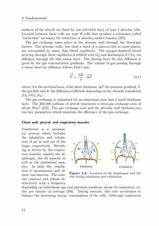
ExhalationInhalation
Figure 2.4: Location of the diaphragm and theribs during inhalation and exhalation.
Ventilation is a mechani-cal process which includesthe inhalation and exhala-tion of air in and out of thelungs, respectively. Breath-ing is driven by the respira-tory muscles, namely the di-aphragm, the rib muscles aswell as the abdominal mus-cles. In daily life, ventila-tion is spontaneous and al-most unconscious. The mus-cles contract and release in-stinctively with a frequencydepending on individuals age and physical condition, about 16 respiratory cy-cles per minute on average [206]. During exercise, this rate accelerates tobalance the increasing energy consumption of the cells. Although respiration
12

2.1 Physiological background
is mostly spontaneous, it is possible to control the driving muscles and thusour breathing rate and amplitude with some effort.The diaphragm is located under the pulmonary compartments and closes the
thorax cage in a convex shape with its highest point at rest position (Fig. 2.4).The rib muscles resting position corresponds to the functional residual capacity(FRC) of the lungs. During inspiration, the respiratory muscles contract. Thediaphragm flattens and stretches, while the ribs move out and open the chestleading to an increased volume available for the lungs. A forced expiration canbe achieved by an additional contraction of the abdominal muscles.
lung compliance
Alveoli
Air
chestwall
compl.
pleural space muscles
Nose
Airways
Figure 2.5: Technical abstrac-tion of lungs, chest wall, and pleu-ral space.
The lungs are located in the thorax cav-ity. The pleural space is the potential spacelocated between the parietal and the vis-ceral pleural. It functions as a mechani-cal coupling which transfers and regulatesthe pressure inside and outside of the lungs(Fig. 2.5). Since the lungs are only sus-pended at the hilum from the mediastinumwithout any other attachment to the chestwall, the lungs float in a waterbed createdby the pleural fluid, which is 8− 12mL or0.3mLkg−1 in volume [135]. The process offluid filtration from from the pulmonary cap-illaries to lung interstitium is normally keptin equilibrium regarding the Starling equa-tion [197]. The heart, in turn, is embeddedin the pleural space via the pericardium, arelatively stiff covering. From the heart, thepulmonary artery and the aorta lead bloodto the pulmonary and body circulation. Re-fluxing blood passes back into the heart viathe pulmonary vein and the superior vena cava.
2.1.2 Respiratory mechanics
The contraction of the respiratory muscles causes a decrease in the pleuralpressure (approximately equal to −7.5cmH2O1 during spontaneous inspira-tion [68]). As a result, the alveolar pressure decreases and air is driven into thelungs through the upper airways. During passive expiration, the respiratorymuscles relax, and the elastic recoil pressure of the lung presses the air out of
11cmH2O = 98.0665N/m2
13

2 Fundamentals
Inspiratoryreservevolume
Expiratoryreservevolume
Tidalvolume
Residualvolume
Funtionalresidualcapacity
Vitalcapacity
Totallung
capacity
Lung volume (% TLC)
100
0
45
52
20
Figure 2.6: Anatomy and technical abstraction of respiratory mechanics.
the lungs. At functional residual capacity (FRC), the pleural pressure Ppl isslightly negative (about −5cmH2O). This pressure is generated by the oppos-ing elastic forces of the chest wall and lung between the visceral and parietalpleura.
Lung volumina
Lung volumes and lung capacities refer to the air volume associated with differ-ent phases of the respiratory cycle. The total lung capacity (TLC) is defined asthe gas volume in the lungs after a maximal inspiration. The residual volume isthe volume remaining in the lungs after a maximal expiration. The differencebetween TLC and the residual volume is called the vital capacity (VC). For astandard adult male, VC is about 80% of TLC. The functional residual capacity(FRC) is the gas volume in the lungs after a normal expiration (Fig. 2.6).
Forces involved in breathing and respiratory parameters
Forces involved in breathing were first described by Otis et al. in 1950 [156] andcompleted by Mead in 1961 [127]. The respiratory system can be modeled bythree different parts: the thorax, the lungs shaped by the pulmonary tissuesand the gas inside the alveoli and airways. These three components form amechanical system whose equilibrium point corresponds to the full respiratorymuscle release and the absence of gas flow at the functional residual capacity(FRC). The respiratory cycle is driven by the muscles, which overcome op-posing elastic forces of lung parenchyma to create the displacement from the
14
2.1 Physiological background
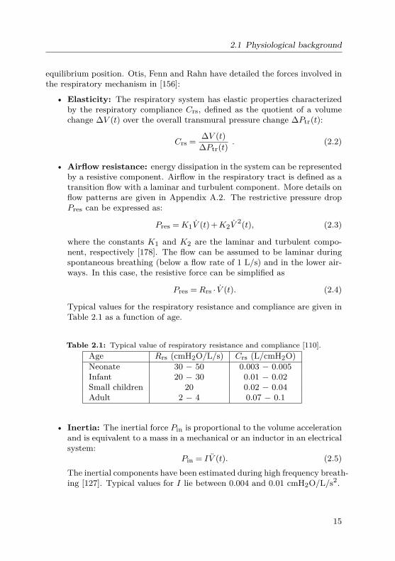
equilibrium position. Otis, Fenn and Rahn have detailed the forces involved inthe respiratory mechanism in [156]:
• Elasticity: The respiratory system has elastic properties characterizedby the respiratory compliance Crs, defined as the quotient of a volumechange ∆V (t) over the overall transmural pressure change ∆Ptr(t):
Crs = ∆V (t)∆Ptr(t)
. (2.2)
• Airflow resistance: energy dissipation in the system can be representedby a resistive component. Airflow in the respiratory tract is defined as atransition flow with a laminar and turbulent component. More details onflow patterns are given in Appendix A.2. The restrictive pressure dropPres can be expressed as:
Pres =K1V (t) +K2V2(t), (2.3)
where the constants K1 and K2 are the laminar and turbulent compo-nent, respectively [178]. The flow can be assumed to be laminar duringspontaneous breathing (below a flow rate of 1 L/s) and in the lower air-ways. In this case, the resistive force can be simplified as
Pres =Rrs · V (t). (2.4)
Typical values for the respiratory resistance and compliance are given inTable 2.1 as a function of age.
Table 2.1: Typical value of respiratory resistance and compliance [110].Age Rrs (cmH2O/L/s) Crs (L/cmH2O)Neonate 30 − 50 0.003 − 0.005Infant 20 − 30 0.01 − 0.02Small children 20 0.02 − 0.04Adult 2 − 4 0.07 − 0.1
• Inertia: The inertial force Pin is proportional to the volume accelerationand is equivalent to a mass in a mechanical or an inductor in an electricalsystem:
Pin = IV (t). (2.5)The inertial components have been estimated during high frequency breath-ing [127]. Typical values for I lie between 0.004 and 0.01 cmH2O/L/s2.
15

2 Fundamentals
Pressure-Volume Diagrams
Mechanical properties of the respiratory system can be characterized by thepressure-volume (PV) diagrams. We distinguish the static PV curve fromthe dynamic PV curve due to the dynamics of the measurement conditions(Fig. 2.7).The static PV diagram is reconstructed under quasi-static conditions. Static
states, approximated by negligible airflow resistance and convection effects canbe measured when airflow is slow or during short apnea time. The static di-agram can be obtained by different methods such as the super syringe, theconstant flow, or the ventilator method [74]. The PV static curve of the respi-ratory system, characterized by an S-shape with a linear domain in the normalbreathing range and concavity at the extremities, is a combination of the chestwall and lung reaction. The downward concavity for high pressure and volumerepresents the limits of the lung tissue elasticity while the chest wall confers thenon-linearity in the low-pressure range. The static compliance Cstat determinesthe lung volume variation for an unit change in pressure.The dynamic PV loop describes the behavior of pressure and volume during
breathing. It is characterized by an hysteresis between inspiration and expi-ration phase. The diagram extremities correspond to the tidal volume for thehigher point and the functional residual volume as the origin.
FRC
VT
Volume (L)
Pressure (cmH O)2
Inspiration
Expiration
-6-5-4
Static curve
TLC
Palv
C = V/ PΔ Δstat
V
RV
FRC
Lungs + Chest
Chest Lungs
0
PΔ
VΔ
Pressure (cmPressure (cmH O)2Pressure (cm20-20
Figure 2.7: Left: Static pressure-volume (PV) relationship of the respiratorysystem, adapted from [221]. Right: dynamic PV diagram, modified from [68].VT = tidal volume.
2.1.3 Physiology of heart, circulation, and lymphaticsThe respiratory system coordinates with the cardiovascular system to maintainthe transport of oxygenated blood to the organs. The cardiovascular system
16

2.1 Physiological background
consists of the heart, the pulmonary and systemic circulation, and the lym-phatic system.
Heart
The heart consists of four chambers: two atria and two ventricles. The atriaproduce low pressures and serve the ventricles mainly as blood stores. Theright (RV) and left ventricle (LV) volumes are encircled by cardiac muscletissue, the "myocardium". Their coordinated contractions pump blood out ofthe chambers to the blood vessels. The dividing wall between the left and rightventricles of the heart is called the (ventricular) septum, which also consistsof cardiac muscles. The entire heart is surrounded by a passive, relatively stiffpericardium, which gives the heart stability and protection from overstretching.There are four heart valves that separate the ventricles from the atria and fromthe arteries and arrange the direction of blood flow in the body. The tricuspidvalve separates the right atrium from the right ventricle and prevents refluxof blood from the ventricle into the atrium. The right ventricle is connectedto the pulmonary artery via the pulmonary valve. Similarly, the left ventricleis connected to the left atrium via the mitral valve and to the aorta via theaortic valve. The pressure arising during the systole is dependent on the fillingvolume of the ventricles (Frank-starling mechanism).The heart cycle is described by a loop bounded by the end-diastole pressure-
volume relationship (EDPVR) and the end-systole pressure-volume relation-ship (ESPVR). While EDPVR represents the elasticity of the ventricles, ES-PVR describes the ventricular contractility. A heart cycle is divided into fourcardiac action phases: a) isovolumetric contraction, b) ventricular ejection, c)isovolumetric relaxation, and d) ventricular filling. The first two phases aresummarized as systole and the second two ones as diastole. The individualphases are presented in the pressure-volume diagram of the heart (Fig. 2.8).During the isovolumetric contraction, the sinus node stimulates the contrac-
tion of cardiac muscles that produce a high ventricular pressure, while fourheart valves are closed. As soon as this ventricular pressure exceeds the corre-sponding arterial pressure, the pulmonary and aortic valves are opened, causinga large blood flow to the arteries (ejection phase). During the isovolumetricrelaxation, the heart muscle relaxes and the ventricular pressures decrease (re-laxation phase). When the ventricular pressures underlie the venous pressures,the tricuspid and mitral valves open and the ventricles fill again with blood fromthe atria (filling phase) [68,96]. The volume difference between the contractionand the relaxation phase is the cardiac stroke volume (SV) of the ventriclesand typically ranges between 70 and 100 mL in the adult humans [68]. Theproduct of pulse and SV defines the cardiac output (amount of blood flowing
17

2 Fundamentals
Ventricular Volume
Ven
tric
ula
r P
ress
ure
ES
PV
R
Outlet valve closure
Inlet valve opening
Inlet valve closure
Outlet valve opening
EDPVR
Ejection
Rel
axat
ion
Contr
acti
on
Filling
Figure 2.8: PV-diagram of the heart, modified from [76].
through the blood circuits per minute). An SV of 75 mL and a pulse of 80beats per minute (bpm) results in a cardiac output of 6 L/min.
Systemic and pulmonary circulation
The human circulation system consists of the systemic and pulmonary circula-tion. Each is, in turn, divided into arteries, capillaries and veins according tothe functionality of the blood vessels (Fig. 2.10 left panel). The systemic circuitdescribes the transport of oxygenated blood from the left ventricle to the or-gans. For a rapid transport, the arterial pressure is high, typically 163cmH2O(120mmHg) systolic and 109cmH2O (80mmHg) diastolic in the aorta [68].The arteries are characterized by a thick elastic wall with a thickness of upto 2.5mm [96]. Systemic arteries branch to smaller arteries and to arterioles,before opening into capillaries. The capillary wall is extremely thin, consist-ing of only an endothelial layer to allow for an effective gas exchange. Afterdelivering oxygen and absorbing carbon dioxide, blood flows though the veinsback to the right atrium. The veins are a thin-walled and low-pressure sys-tem. Their compliance is high so that a large amount of blood can be stored.The systemic veins stores approximately 60% of the total blood volume in thehuman body [68,96,184].While the pulmonary circulation has a similar structure to that of the sys-
temic one, the pulmonary blood pressure is significantly less. Pulmonary arte-rial pressure is about 34cmH2O (25 mmHg) in systole and 11cmH2O (8 mmHg)in diastole. The mean capillary pressure in the lungs is about 10cmH2O. Themedian pressure drop in the pulmonary circulation is about 19cmH2O. This
18

2.1 Physiological background
a c v
Diastole Systole
Volu
me
(ml)
Ejection
Pre
ssure
(m
m H
g)
Systole
Isovolumicrelaxation
A-Vvalveopens
Atrialsystole
Rapidinflow
Diastasis
Ventricular pressure
Aortic pressure
Atrial pressure
Ventricular volume
Isovolumiccontraction
Aorticvalvecloses
Aorticvalveopens
A-Vvalvecloses
Figure 2.9: Events of the cardiac cycle for left ventricular function pressure, leftventricular pressure, aortic pressure and ventricular volume. Adapted from [68].
value results in a pulmonary flow resistance of Rpul = 190cmH2OL−1 s, for acardiac output of 6 L/min. Analogously, the flow resistance of the systemic cir-culation can also be determined to be around Rsys = 1330cmH2OL−1 s [68,96].
Lymphatic system
The human circulatory system processes an average of 20 L of plasma per daythrough capillary filtration. While 17 L are reabsorbed directly back to thevessels, the other 3 L remain in interstitial space and are later returned tothe blood by the lymphatic system (Fig. 2.10, right top figure). The lymphat-ics comprise a network of lymphatic capillaries, collectors, nodes, and largerstrains that carries fluid from interstitial spaces towards the vena cava superior.In the lungs, a lymphatic capillary network of about 50 · 10−6 m in diametercrosses the interstitial space. Unlike the cardiovascular system, the lymphaticsystem has no central pump. Lymph movement occurs due to contraction andrelaxation of the lymphatic collectors, valves, and compression during adjacentskeletal muscles’ contraction [187]. Lymphatic collectors have a similar struc-ture to the systemic veins: They consist of smooth muscles which contract asa forward fluid pump; and they are separated by lymphatic valves which allowa unidirectional flow of fluid [138, 184]. From lymphatics collectors, fluid istransported to lymph nodes and large lymphatic strains, before returning to
19

2 Fundamentals
Cerebral and upper-limbcapillaries
Pulmonarycapillaries
Vena cava superior
Pulmonaryartery
Left atrium
Aorta
Left ventricleRight ventricle
Intestine
Liver
Pulmonaryvein
Right atrium
Lymph node
Vena cava inferior
Systemic vein
Body and lower-limbcapillaries
lymph capillaries
lymph collectors
lymph nots
lymphatic duct
Vena cava superior
Liq
uid
relaxing segment
Interstittium
proximal valve
contracting segment
distal valve
Figure 2.10: Left: The circulation system. Right top: fluid transport in thelymphatic system. Right bottom: a lymphatic collector, modified from [184].
the vena cava superior. Figure 2.10 right figures illustrate the components ofthe lymphatic system and the structure of a lymph collector.
2.2 Pulmonary function diagnostics
Pulmonary function tests are elementary diagnostic tools in pneumology. Apulmonary function test (PFT) is ordered by a doctor as a part of a routinephysical check-up to examine the presence of lung pathologies or to assess thestatus of the lungs prior to medical treatment or surgery. In general, PFTscan be divided into direct and indirect measurement techniques [110], as il-lustrated in Fig. 2.11. Direct PFTs, comprising of the esophageal catheter,the interrupter and the forced oscillation technique, measure mechanical pa-rameters such as resistance, compliance, or impedance. Indirect PFTs providesinformation about subdivisions of lung volumes via spirometry, helium dilution,nitrogen washout, or diagnostic images via radiography, computer tomography,or magnetic resonance imaging. The body plethysmography provides both lungvolumes and airway resistance, thus, belongs to both categories.With exception of the imaging techniques, PFTs generally involve uncovering
relationship between pressure, flow, and volume measured at the airway open-
20

2.2 Pulmonary function diagnostics
Pulmonaryfunction tests
Direct methods:assessment of lung mechanics
Esophagealcatheter
Indirect methods:measurement of lung volume
F ,RV (ITGV)
RC
Helium dilution/Nitrogen washout
Bodyplethysmography
InterrupterForced
oscillationSpirometry
Volume relatedimages
ZrsRintCrsRaw
Imagingtechniques
(Radiograph,CT,
MRI)
FV loop, FEV ,FVC, Tiffeneau-index
Figure 2.11: Pulmonary function testing (modified from [110]).
ing. Spirometry, FOT and interrupter are noninvasive techniques with simplemeasurement setup where data are captured only at the airway opening of thetest subjects. In contrast, the esophageal catheter requires that the subjectsswallow a balloon catheter during the test, which makes this technique invasiveand unpratical in use. Body plethysmography, helium dilution, and nitrogenwashout are more complex and expensive in installation, thus are often onlyavailable in clinics or pulmonary laboratories.Standard guidelines of pulmonary function testing in adults and children
are given by the European Respiratory Society (ERS) and American ThoracicSociety (ATS) with the latest series of papers for adults and children pub-lished in 2005 [132, 133, 162, 218]. For infants, a series of seven articles havebeen carried out by the ATS/ERS Task Force in 2000 [13,59–61,137,190,198].In 2007, an ATS/ERS consensus statement on pulmonary function testing inpreschool children, mostly based on personal experiences [19], was published.ATS and ERS recommend the measurement of lung volumes during a spirom-etry test (forced vital capacity (FVC), forced expiration volume (FEV), andTiffeneau-index), in combination with a bronchodilator or bronchial challengetest as the standard method to assess lung function in adults and children.Advanced PFTs require a higher level of system understanding and instrumen-tation [183]. Body plethysmography efficiently combines the measurement ofresidual lung volume and airway resistance and is considered as the gold stan-dard for measurement of airway resistance. However, it should be noted thatthere is no standardization recommended by ERS/ATS for the use of directparameters such as resistance or compliance to assess lung pathologies. Major
21
2 Fundamentals
difficulties are the strong variation between measurement values among meth-ods and devices, the invasiveness (in esophageal catheter technique), or thedifficult interpretation of the measurement results (in FOT).
2.2.1 Spirometry
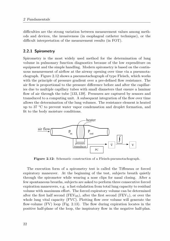
Spirometry is the most widely used method for the determination of lungvolume in pulmonary function diagnostics because of the low expenditure onequipment and the simple handling. Modern spirometry is based on the contin-uous measurement of airflow at the airway opening over time via a pneumota-chograph. Figure 2.12 shows a pneumotachograph of type Fleisch, which workswith the principle of pressure gradient over a pre-defined flow resistance. Theair flow is proportional to the pressure difference before and after the capillar-ies due to multiple capillary tubes with small diameters that ensure a laminarflow of air through the tube [133, 139]. Pressures are captured by sensors andtransduced to a computing unit. A subsequent integration of the flow over timeallows the determination of the lung volumes. The resistance element is heatedup to 37 °C to prevent water vapor condensation and droplet formation, andfit to the body moisture conditions.
p p
V
outin
air flow
PC
pressuretransducer
V.
heater
Figure 2.12: Schematic construction of a Fleisch-pneumotachograph.
The execution form of a spirometry test is called the Tiffeneau or forcedexpiratory maneuver. At the beginning of the test, subjects breath quietlythrough the spirometer while wearing a nose clips for nasal closing. After afew spontaneous breaths, subjects are asked to perform three consecutive forcedexpiration maneuvers, e.g. a fast exhalation from total lung capacity to residualvolume with maximum effort. The forced expiratory volume can be determinedafter the first half second (FEV05), after the first second (FEV1), or over thewhole lung vital capacity (FVC). Plotting flow over volume will generate theflow-volume (FV) loop (Fig. 2.13). The flow during expiration locates in thepositive half-plane of the loop, the inspiratory flow in the negative half-plan.
22

2.2 Pulmonary function diagnostics
MEF
PEF
50
MEF75
MEF25
Flo
w
Volume75% 50% 25%
FVC RV
Forced expiration
Inspiration
Volu
me
Time (s)
0.5s1s
FEV1
FEV0.5
RV
FVC
Figure 2.13: The flow-volume loop and the spirometric parameters.
Lung pathologies hide in the form of FV loops, as shown in Fig. 2.14.
a) Normal loops
No forcedexpiration
Good No maximumexpiration
e) Emphysema
b) Restriction
HeavyModerate
d) Stenosis
Fixed extra-thoracic sternosis
Intrathoracictracheal stenosis
c) Obstruction
Figure 2.14: Illustration of different ventilation disorders in the flow-volumeloop, redrawn from [183].
The Tiffeneau index (TI), calculated as the ratio FEV1/FVC, serves as
23

2 Fundamentals
a means of diagnosing lung diseases. According to the Global Initiative forChronic Obstructive Lung Disease (GOLD), a TI of less than 0.7 is alreadyan indication for COPD [160]. A second indicator for lung pathologies is thevalue of FEV1 in percentage of the predicted reference value. This value isdetermined by means of regression equations regarding age, body height, andweight of the patient. Other diagnostic parameters are peak expiratory flow(PEF), as well as maximum expiratory flow at 75%, 50%, and 25% of FVC(MEF75, MEF50, and MEF25, respectively). While the expiratory part of thehealthy patient’s loop shows a linear gradient, the asthmatic one has a concavedrop (Fig. 2.14) [139]. This concavity becomes more pronounced depending onthe severity of the obstruction.The bronchodilator test utilizes spirometry to assess possible reversibility
of bronchoconstriction in diseases such as asthma. Spirometry measurementsare performed before and after the patients taking a dose of bronchodilatormedication (such as 400 µg of salbutamol). An increase in FEV1 of > 12% isconsidered a positive result.
2.2.2 Helium dilution and nitrogen washout methodsHelium dilution and nitrogen washout methods are pulmonary function testswhich determine the functional residual capacity (FRC) of the lungs. Both havebeen standardized by the ATS/ERS [218]. The helium dilution technique isbased on the idea that helium does not diffuse from the alveoli into the bloodand thus is not affected by the gas exchange. During the test, the patientinhales a predefined helium volume in addition to the inhaled air. FRC is com-puted from the proportion of helium concentration before and after inhalationin the lungs [110,218]:
FRC = Vcontainer[He]before− [He]after
[He]after(2.6)
The second technique is based on washing out N2 from the lungs, while patientsinhale 100% O2. Lung volume at the start of washout can be calculated by theamount of N2 washed out and the initial alveolar N2 concentration [218].
2.2.3 Body plethysmographyThe (whole) body plethysmography was introduced by DuBois in 1956 [42].Besides the measurement of spirometric parameters, it provides the effectiveairway resistance (Raw), the specific respiratory resistance (sRaw), and thethoracic gas volume (TGV) [62,110]. While the measurements require trainedmedical personal, the patients’ effort is reduced compared to spirometry.
24

2.2 Pulmonary function diagnostics
Rtan α p
b
pao
pao
pm
pp
ao
pb
pb
pb
box pressure
mouth pressure
[kPa/cmH O]2
=
VL
aw
FRC
shutter closed
[mL]
pb
pb
pb
box pressure
flowV.
[L/s]
tan β pb
=V.
VLVL
Raw
FRC
V.
shutter open
[mL]
V.
Figure 2.15: Determination of the airway resistance Raw with the bodyplethysmography, modified from [35]. Top: shutter open, respiratory loop ofairway flow against cabin pressure. Bottom: shutter closed, shutter-maneuverloop of airway pressure pao against cabin pressure pb.
The plethysmograph is a hermetically sealed cabin with an integrated pneu-motachograph and a shutter. The box has a defined volume of air and aminimal leakage for pressure compensation caused by patient’s body heat.During the test, the patient breathes quietly through a pneumotachograph,while flow, airway and cabin pressures are recorded. During inhalation, thepatient’s ribcage rises, the cabin volume falls and the box pressure increases.The intrathoracic gas volume (IGV) can be determined by the law of Boyle-Mariotte for isothermal gas (P ·V = const) [62, 110]. Considering the watervapor partial pressure in the lungs, pH2O = 6.27kPa, IGV can be computed as:
IGV =∆Vlung∆pao
· (patm−6.27kPa) (2.7)
The change in lung volume ∆Vlung is not directly measurable and can bereplaced by the product of the box pressure drop ∆pb and a calibration constantKbody:
IGV = ∆pb∆pao
·Kbody · (patm−6.27kPa) (2.8)
25

2 Fundamentals
During spontaneous breathing, an installed shutter is activated. The subjectcontinues his normal breathing against the shutting valve. Since there is nopressure drop along the resistance element at that time, the alveolar pressure isequal to the mouth pressure. Plotting the flow and the airway pressure againstthe box pressure gives us the respiratory loops of the body plethysmography(Fig. 2.15). The airway resistance Raw is computed as
Raw = tanαtanβ (2.9)
where α and β are obtained from the two respiratory diagrams. The specificairway resistance sRaw is the product of the airway resistance and the func-tional residual capacity (FRC) of the lungs:
sRaw =Raw ·FRC. (2.10)
An alternative body plethysmography introduced by Mead in 1960, measureslung volume change directly by having subjects breath in and out across thewall of the box [126]. Although Mead’s body plethysmography provides thelung compliance as an additional parameter, calibration and execution of themeasurements are more difficult compared to the DuBois’s version. Mead’smethod is not widely used in the praxis nowadays.
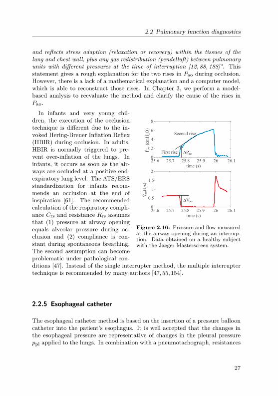
2.2.4 Rapid interrupter techniqueThe rapid interrupter technique (or occlusion technique) was first introducedby Von Neergaard and Wirz in 1927 [215]. This technique relies on the factthat during a sudden airflow interruption at the airway opening, alveolar andmouth pressure will rapidly equilibrate. Figure 2.16 shows the pressure andflow obtained at the airway opening of a healthy subject. The interrupter wasactivated during a spontaneous inspiration. Two rises in Pao can be observed.The respiratory resistance is computed as the quotient between the pressuredrop immediately before and after closing the valve, and the flow at airwayopening immediately before closing:
Rint = ∆PaoVao
(2.11)
In the ATS/ERS statement on pulmonary testing in preschool children [19],the authors commented on the first rise Pinit and the second rise Pdiff of thepressure as follow: "During tidal breathing, Pinit, and thus Rinit, will includea component of both lung tissue and chest wall resistance, not only airwayresistance. Pdiff is due to the viscoelastic properties of the respiratory tissue
26
2.2 Pulmonary function diagnostics
and reflects stress adaption (relaxation or recovery) within the tissues of thelung and chest wall, plus any gas redistribution (pendelluft) between pulmonaryunits with different pressures at the time of interruption [12, 88, 188]". Thisstatement gives a rough explanation for the two rises in Pao during occlusion.However, there is a lack of a mathematical explanation and a computer model,which is able to reconstruct those rises. In Chapter 3, we perform a model-based analysis to reevaluate the method and clarify the cause of the rises inPao.
25.6 25.7 25.8 25.9 26 26.10
2
4
6
8
time (s)
(cm
H2O
)
25.6 25.7 25.8 25.9 26 26.10
0.5
1
1.5
2
V(L
/s)
aoao
P
time (s)
˙ΔVao
ΔPaoFirst rise
Second rise
Figure 2.16: Pressure and flow measuredat the airway opening during an interrup-tion. Data obtained on a healthy subjectwith the Jaeger Masterscreen system.
In infants and very young chil-dren, the execution of the occlusiontechnique is different due to the in-voked Hering-Breuer Inflation Reflex(HBIR) during occlusion. In adults,HBIR is normally triggered to pre-vent over-inflation of the lungs. Ininfants, it occurs as soon as the air-ways are occluded at a positive end-expiratory lung level. The ATS/ERSstandardization for infants recom-mends an occlusion at the end ofinspiration [61]. The recommendedcalculation of the respiratory compli-ance Crs and resistance Rrs assumesthat (1) pressure at airway openingequals alveolar pressure during oc-clusion and (2) compliance is con-stant during spontaneous breathing.The second assumption can becomeproblematic under pathological con-ditions [47]. Instead of the single interrupter method, the multiple interruptertechnique is recommended by many authors [47,55,154].
2.2.5 Esophageal catheter
The esophageal catheter method is based on the insertion of a pressure ballooncatheter into the patient’s esophagus. It is well accepted that the changes inthe esophageal pressure are representative of changes in the pleural pressureppl applied to the lungs. In combination with a pneumotachograph, resistances
27

2 Fundamentals
of the lungs and thorax are given as follow:
Raw =ppl(t)−pmouth(t)
V (t)(2.12)
Rcw =pmus(t)−ppl(t)
V (t)(2.13)
Pes
V.
Sensor
Figure 2.17: Measure-ment principle of theesophageal method.
Dependent on the breathing mode, eithereq. (2.12) or eq. (2.13) can be applied. During spon-taneous breathing, the pressure at airway openingis equal to the atmospheric one pmouth = patm whilepmus remains unknown. Hence, the airway resistanceRaw can be computed regarding eq. (2.12). Duringmechanical ventilation, the respiratory muscles areinactive pmus = 0, eq.(2.13) can be applied to cal-culate the chest wall damping Rcw. Note that thetissue resistance Rti is included in the airway resis-tance Raw in eq.(2.12).The accuracy of the esophageal catheter technique
depends strongly on the correct localization of theballoon. Furthermore, the method is invasive, sinceeither the patient needs to swallow the balloon or itis inserted through his nose. Although this techniquecan be useful for monitoring the intra-thoracic pressure during mechanical ven-tilation, the practical use of the esophageal catheter is limited. It has been usedmostly in former clinical studies and animal trials.
2.2.6 Forced Oscillation TechniqueThe Forced Oscillation Technique (FOT) was first introduced by DuBois et al.in 1956 [43]. This noninvasive method is based on external small-amplitudeoscillatory signals applied at the patient’s mouth and superimposed on thespontaneous breathing. The oscillation signals can be sinusoidal (FOT), im-pulse (Impulse Oscillometry), or noise (Pseudo Random Noise). The absence ofpatient’s cooperation necessity makes FOT attractive for examination duringsleep, in infants or when breathing is difficult to control. Technical recom-mendations and clinical practice of this method is given in the ERS guidelinespublished in 2003 [155].In FOT, the sinusoidal signals can include single or multiple frequencies.
Measurements are conducted simultaneously to spontaneous breathing becausethe frequencies used are mostly more than 10 times higher than the respiration
28

2.2 Pulmonary function diagnostics
rate and thus, can be easily separated from the respiratory rate. Due to linear-ity requirement of spectral analysis, FOT signals should remain in a relativelysmall amplitude range [119,155].Respiratory mechanical parameters are then assessed by spectral analysis
of the resulting flow and pressure recorded at the patient’s airway opening.The respiratory impedance Zrs defined as the spectral ratio of the measuredpressure and flow signals is divided into a resistance and reactance part:
Zrs(jω) = Pao(jω)Vao(jω)
= Zrs,R(ω) + jZrs,X(ω), (2.14)
where ω is the oscillatory frequency. The resistance Zrs,R describes the pressure-flow fraction of the part of the pressure signal in phase with the flow. The reac-tance Zrs,X represents effects of both elastic and inertial forces which create aphase shift between pressure and flow signal [63]. At lower frequencies, Zrs,X isdominated by elastic components. Above the resonance frequency fres, inertiahas a stronger impact on the impedance [54].
Reacta
nce
(kP
as/
L)
10 20300Frequency (Hz)
1
0
healthyairway obstruction
resonance frequency
10 200
Resi
stance (
kP
a s
/L)
0
Frequency (Hz)
1
healthyairway obstruction
3030
Figure 2.18: Resistance (left) and reactance (right) with respect to frequencymeasured with FOT, redrawn from [155].
Different studies have established impedance resistance disparities betweenhealthy subject and individuals suffering from obstructive lungs diseases [73,209] (Fig 2.18). In acute asthma, FOT may prove to be useful for assessingbronchodilator response [44, 155]. However, a study in preschool children re-ported only a marginal correlation between the resistive impedance at 8 Hz andthe asthma severity ratings [26]. FOT measurements also exhibit a poor cor-relation with the spirometric indices in children with cystic fibrosis [79, 195].Hence, for FOT, the systematic relationship between the impedance Z(jω)measured with FOT and other lung function parameters such as FEV1 and
29

2 Fundamentals
Rint has not been understood. There is a lack on the physiological interpreta-tion of the respiratory impedance Z(jω).
2.3 Mechanical ventilation
Mechanical ventilation is the medical treatment where a technical machine isused to assist or replace spontaneous breathing. Mechanical ventilation hasfour main goals: (1) delivering oxygen to the alveoli, (2) removing carbondioxide from the lungs, (3) providing mechanical work of breathing, and (4)maintaining pressure and volume in patients’ lungs. Ventilators are most oftenused during surgery with general anesthesia, or for patients with impaired lungfunction (Pneumonia, COPD, ARDS, etc). In the 19th and 20th centuries, neg-ative pressure ventilators or the iron lungs were widely used. The iron lung isa hermetically scaled metal chamber surrounding the patient’s body with sub-atmospheric pressure for lung expansion [92, 113, 121]. Since the developmentof positive pressure ventilation and the intensive care unit in the 1960s, morethan 174 different ventilation modes have been developed [134]. They can beclassified in two main categories: assisted spontaneous breathing (ASB) andcontrolled-ventilation.
2.3.1 Continuous positive airway pressure (CPAP)
Pre
ssure
Normalbreathing
Normalbreathing+ CPAP
BiPAP
PEEP
BiPAP-supportedpressure
Time
PEEP
Figure 2.19: Spontaneous breathing,CPAP, and BiPAP.
A typical form of ASB is the ContinuousPositive Airway Pressure (CPAP), whichapplies a mild pressure on top of sponta-neous breathing to keep the airways con-tinuously open. CPAP is typically usedfor patients with obstructive sleep apneaand/or heart failure during sleep, usu-ally through a nasal mask. Another formof CPAP with a pre-defined level of in-spiration is the Biphasic Positive AirwayPressure (BiPAP) mode, as illustrated inFig. 2.19.
2.3.2 Pressure- andvolume-controlled ventilationPressure- and volume-controlled ventilation (PCV and VCV) are different con-trol variables within a mode. In VCV, tidal volume is pre-set manually,while PCP allows the adjustment of ventilation pressure (positive inspiratory
30

2.4 Electrical Impedance Tomography
pressure PIP and positive end-expiratory pressure PEEP). A mixed form isthe pressure-regulated volume control, which applies VCV with an additionalpressure-limited control. This form ensures a consistent tidal volume for dy-namic alteration of lung mechanics during mechanical ventilation, and monitorsthe maximal pressure to reduce the risk of ventilation-induced lung injury.
2.4 Electrical Impedance Tomography
Electrical Impedance Tomography (EIT) is a noninvasive, radiation-free imag-ing technique which is based on the measurement of cross sectional impedancedistribution of biological tissues. The response of a material exposed to exter-nal electric field depends on its electrical properties such as conductivity σ andpermittivity ε:
γ(x,ω) = 1z(x,ω) = σ(x) + jωε(x), (2.15)
where γ is the admittivity, the inverse of the impedivity z, x is the position con-sidered in the material and ω the excitation pulsation. Impedance tomographydetermines the impedance distribution inside the material using informationmeasured at the element boundaries. Electrodes placed at the object circumfer-ence repeatedly send small alternating electrical currents while measuring theresulting surface voltages. The transfer impedances obtained are used to re-solve the inverse problem of the distribution using to numerical reconstructionmethods [22].The first transmission image of the chest based on the impedance was in-
troduced by Henderson and Webster in 1976. The measurement system had a100-electrode matrix coupled with a single large electrode on the back and thefront of the thorax, respectively [80]. In 1983, Brown et al. published the firsttomographic images using current injection between adjacent electrodes withonly 16 electrodes [6]. Since then, his method has been continuously studiedand developed to enlarge the application fields and enhance the performance.EIT has become a very promising tool in bedside monitoring of lungs ventila-tion and perfusion [57,73,102,112].In 2011, Dräger Medical GmbH, Lübeck, Germany released the first EIT
device for daily clinical use, the PulmoVista® 500, utilized for patient mon-itoring in intensive care settings. The PulmoVista 500 sequentially appliessmall alternating electrical currents (IEC 60601-1, 80−130kHz, automaticallyadjusted amplitude at approximately 5mA) through a pair of the 16 electrodesattached to a belt on the circumference of the patient’s chest, and measuresthe difference of voltage between the remaining electrode pairs (Fig. 2.20 left).For each frame, 208 differential voltages are recorded, of which 104 are linearly
31

2 Fundamentals
1 2
3
4
5
6
7
8910
11
12
13
14
15
16
IV
V
V
V
V
VVV V
V
V
V
V
V
10 cm
10 cm
0.5
0.3
0.1
0.9
0.5
0.3
0.1
Figure 2.20: Left: Sequence of current injection and voltage measurement.Right: Effect of distance in impedance calculation.
independent due to reciprocity. The electrical impedance Z is obtained as themeasured voltage V over the injected current I (Z(t) = V (t)
I(t) ).
Figure 2.21: A reconstructedEIT image (32x32 pixel).
An integrated finite-element-method basedon the linearized Newton-Raphson recon-struction algorithm can be used to recon-struct EIT images from the raw voltage sig-nals (Fig 2.21). One image is obtained whenall electrode pairs have been used to in-ject current. In general, around 10 cm overand below the electrode plane can be de-tected with EIT devices (Fig. 2.20, rightpanel) [203].Once EIT images have been reconstructed,
each pixel value of the 32x32 images is equalto the impedivity variation at this point withrespect to a reference, which is the rela-tive impedance value for each pixel (calledimpedance index or relative image pixel):
p(x,t) = ∆z(x,t) = z(x,t)−zref(x)zref(x) . (2.16)
The sum over all pixel is called the global impedance index:
∆Z(t) =∑
32x32∆z(x,t). (2.17)
32

2.5 Object-oriented modeling language for biophysical modeling
Many studies have investigated the relation between impedance values andpulmonary ventilation. In the 80s, Harris et al. showed that the globalimpedance index was highly correlated with the volume of air contained insidethe lungs [73], which was confirmed later by different research groups [57, 82].In other words, the global impedance index can be linearly interpolated bythe spirometry measurement obtained at the airway opening. Thanks to thisrelationship, it is possible to assess the airflow inside the lungs with EIT data.Other researchers have also highlighted the local information given by EIT
through the comparison of the right and left lung behavior [57,58]. Serrano etal. identified a volume difference between the compartments consistent withphysiological data (47% to 53% for respectively the left and right lung) [186].Kunst et al. compared EIT left-to-right ratio with radionuclide scanning andattested the reproducibility and reliability of EIT measurements for both per-fusion and ventilation division [102].
2.5 Object-oriented modeling language for biophysicalmodeling
In this thesis, biophysical forward models are programmed in the object-orientedmodeling language (OOML) Matlab Simscape™ . OOML considers energy flowamong the compartments in four-terminal representation [86]. It uses lumpedelements to model physical quantities such as energy sources, storages, trans-formers, converters, and sinks. There are three types of equations in the four-terminal representation: balance, constitutive, and phenomenological equa-tions [86]. The energy inflow, outflow, and storage of a system are describedby balance equations. Constitutive equations characterize the energy flow be-tween two potentials, or in other words, represent the mathematical relationbetween a through-variable (fluid flow, electrical current, chemical concentra-tion changes) and an across-variable (potential, voltage, pressure) [86]. Phe-nomenological equations describe the sinks and losses of energy by dissipativeelements, e.g. due to Ohm’s law or Fick’s law of diffusion.In OOML, each model component is modeled by one or more constitutive
equations (pressure-volume characteristics for compliances) or phenomenolog-ical equations (pressure-flow characteristics for resistance). A representativeexample is the Windkessel model of the vascular system [56] (Fig. 2.22). Bloodfrom the arterial compartment Ca flows through the total peripheral resis-tance of the vascular bed RTPR to the venous compartment Cv. Pa, Pv, Psurare the arterial, venous, and surrounding pressures, respectively. The balance
33

2 Fundamentals
-
+
-
-
resistance R
from heart to heart
venouscompl.C
++
arterialcompl.C
v
v
PC
Va
P
TPR
Psur
PRa
PC
.
VC
.Vv
.
vVC
.
a
a
VR
.
Pa
Pv
total peripheral
Figure 2.22: A simple model of a vascular system.
equations are given as:
Va(t) = VCa (t) + VR(t); VR(t) = VCv (t) + Vv(t)Pa(t) = PCa (t) +Psur(t); Pv(t) = PCv (t) +Psur(t)Pa(t) = PR(t) +Pv(t) (2.18)
The pressure-volume relation of the compliances Ca and Cv are described bythe constitutive equations:
∆PCa,v (t) = 1Ca,v
·∆VCa,v (t), or VCa,v (t) = Ca ·dPCa,v (t)
dt.
The phenomenological equation for the flow resistance RTPR is given as
PR(t) =RTPR · VR(t) (2.19)
In signal-based or text-based programming languages such as Simulink orC++, we need an explicit implementation of the balance equations. In Sim-scape™, these equations can be realized implicitly in the graphical structure ofthe model, thus no explicit implementation is required. In this case, the balanceequations (2.18) are implicitly derived from Fig. 2.22. Electrical equivalent rep-resentation can be applied by replacing hydraulic elements by electrical ones,since pressure, volume, and flow correspond to voltage, charge, and current inthe hydraulic-electrical analogy, respectively (Table 2.2). This simplificationassumes a perfect Newtonian fluid, e.g. constant density and viscoelasticity,within a medium.
34

2.5 Object-oriented modeling language for biophysical modeling
Table 2.2: Correspondence between electrical and hydraulic (cardiorespiratory)units.
Electrical Unit Hydraulic UnitVoltage U V Pressure gradient ∆p cmH2O or mmHgCurrent I A Flow V L/sCharge Q C Volume V LResistance R Ω Flow resistance R cmH2O/L/sCapacitor C F Compliance C L/cmH2OInductance L H Inertance I cmH2O/L/s2
35


3 Respiratory modeling
I’m an adventurer, looking for treasure.Paulo Coelho
This chapter introduces a mathematical multi-compartment model of the res-piratory system. The model is developed in order to gain better understand-ing of respiratory mechanics and lung pathologies. The development of themodel comprises compartmentalization, non-linear characterization of the com-ponents, parametrization, and validation. At the end of the chapter, a model-based analysis for reevaluation of the interrupter technique is presented toexemplarily demonstrate the use of the model.Parts of the chapter were previously published in a peer-reviewed jour-
nals [146].
3.1 Non-linear model components
A lumped model of the respiratory system is a set of ordinary differential equa-tions (ODEs) that describe precisely the behavior of the lungs. With respect tosystem complexity, a compartmentalization of the respiratory tract ensures alumped structure. Figure 3.1 illustrates the abstraction of lung mechanics fromthe physiological view (left) to the physical compartment structure (right).
3.1.1 Airways and airspaces
The human airways are divided into the upper airways and the bronchial treeseparated by the larynx. The bronchi tree is subdivided into central bronchi(first 5 generations, N = 0−4) and peripheral bronchi (next 11 generations, N =5−15). Generations 16−23 (or 16−26 in the Hansen-Ampaya model [71]) shapethe respiratory bronchioles and alveoli. Regarding their mechanical propertiesand physiological functionalities, it is adequate to subdivide the airways andairspaces into three compartments: the central compartment (including up-per airways and central bronchi), the peripheral compartment, and the alveoli(Fig. 3.2).
Volume of the airway/airspace compartments.
The upper airways are small in volume (approx. 70 mL including a nasalvolume of 31mL [207]). Bronchial volume for each generation can be estimatedby the morphometric data of Weibel [219], Hansen [71], or Yeh and Schum [226].
37

3 Respiratory modeling
AlveoliPeripheralbronchi(N = 5 - 15 )
Centralbronchi(N= 0 - 4)
Upperairways
InterstitiumLung tissue
Chest wall
Diaphragm
Pleuraspace Ppl
Palv
Pint
Pao
Mouth / Nose
Pao
Mouth / Nose
Upperairways
Centralbronchi
Peripheralbronchi
Alveoli Chest wall
Pleural space
Lung tissue
Ppl
Ribs
Respiratory muscles
DiaphragmRibs
Air
Pmus
Pint
CentralairwaysPeripheralairways
Figure 3.1: Compartmentalization of the respiratory system. N = generationnumber.
Upperairways
Centralbronchi
Air conducting zoneCentralcompartment
AlveoliPeripheral bronchi
Respiratory zone
Volu
me
< 70 mL incl.nasal passage
N = 5 - 15
50 - 100 mL
(Weibel)
≈2.8 - 4.5 L
(Weibel)
≈50 mL const
(Weibel)
≈
N = 0 - 4 N >15
Figure 3.2: Airway compartments with generation number and volume.
Table 3.1 displays the resulting volume for central and peripheral bronchi aswell as alveoli.The Weibel model proposes a volume of approx. Vc = 49 mL (1.6 %) for the
central bronchi, Vb = 59 mL (2 %) for the peripheral airways, and Valv = 2864(95 %) mL for the alveoli at a total lung gas volume of Vlung = 3 L. IncreasingVlung from 3 L to 4.76 L, the central bronchial volume remains constant, while
38

3.1 Non-linear model components
Table 3.1: Volume of the airway and airspace compartment, regarding thegeometrical structure models of Weibel, Hansen & Ampaya, and Yeh & Schum.Vlung = total lung volume, Vc = volume of the central bronchi, Vb = volume ofthe peripheral bronchi, and Valv = alveolar volume.
Vlung Vc Vb ValvValvVb
(mL) (mL) (mL) (mL)Weibel inspi. 3002 48.73 58.77 2863.5
expir. 4759 50.51 94.09 4583.4∆V 1757 1.78 35.32 1719.9 48.7
Hansen & inspi. 2696.5 49.1 51.9 2564.5Ampaya expir. 3856.7 50.5 74.9 3700.3
∆V 1160.2 1.4 23 1135.8 49.4Yeh & Schum total 5563.88 64.98 162.23 5336.67 32.9
the peripheral bronchi and alveoli compartments expand proportionally to lungvolume. For healthy adults, the fraction Valv/Vb can be considered as constantunder quasi-static conditions, when air flow in system is close to zero:
ValvVb
= const >> 1. (3.1)
This fraction can change dramatically in high dynamic processes such as duringforced expiration maneuvers, where the peripheral bronchi above the equalpressure point (EPP) collapse partly. The concept of EPP, introduced byMead in 1967 [131], explains the existence of a limited maximum flow duringthe forced expiration maneuver.The airway and airspace compliances can be derived for pressure and lung
volume changes, e.g. during spontaneous breathing. As shown in Table 3.1,Weibel and Hansen & Ampaya proposed the following relation between thestatic compliances of the central, peripheral, and alveolar compartments Cc,Cb, Calv:
Cc/Calv = ∆Vc/∆Valv ≈ 0.001≈ 0, (3.2)Calv/Cb = ∆Valv/∆Vb ≈ 30−50. (3.3)
Independent from the works of Weibel and Hansen & Ampaya, Vogel andSmidt proposed the values Calv = 0.2 and Cb = 0.004cmH2O/L/s for normalhealthy subjects [210]. This results in the same fraction Calv/Cb ≈ 50 as re-ported in the Weibel and Hansen & Ampaya models.It seems that the fraction Calv/Cb has not gained much attention in recent
lung researches. However, as shown in later chapters of this work, this fraction
39

3 Respiratory modeling
plays a key role in the simplification of model structure and hence, the inter-pretation of the measurement data obtained with the interrupter and forcedoscillation techniques. Model-based detail analysis will be discussed in laterchapters.
Flow pattern and flow-dependent resistance
The air velocity in the lungs depends on the geometry of the lungs as well asthe applied pressure gradient which creates the air flow. In most situations,gas in the lungs can be considered as Newtonian fluid (incompressible, constantdensity), unless a high thoracic pressure is created by the muscles while themouth is closed. The value of the Reynold number determines if the flowis in laminar, transitional, or turbulent regime. Details on flow patterns areexplained in Appendix A.2.Figure 3.3 depicts the Reynold number against the generation number for
normal (0.1 L/s) and heavy (1.667 L/m) breathing, as reported in [38]. Thenormal breathing rate of 0.1 L/s is calculated by twelve breathings of 0.5 Lin one minute. According to this diagram, the flow in all airways is laminarduring normal breathing. During heavy exercise, while flow in the peripheralairways remains laminar, flow in the central bronchi becomes transitional andturbulent .
0 5 10 15 200
2
4
6
8
10
12
14
Rey
nold
num
ber
(10³)
24Generation number
transitional
turbulent
laminar
Central bronchi Peripheral bronchi Alveoli
Heavy exercise(1.667 L/s)
Normal breathing(0.1 L/s)
Figure 3.3: Reynold number of flow in the bronchial tree. Redrawn from [38].
A more detailed diagram was reported by Pedley et al. in [161], where air-ways resistances were predicted as a function of airway generation regardingthe Weibel model (Fig. 3.4). The diagram proposed a flow-independent resis-tance for small airways (N ≥ 10), and a flow-dependent resistance for largeairways (N ≤ 6) at high flow. The middle airway generations (7−10) belongsto a transitional regime: more airways become flow-dependent when the flow
40
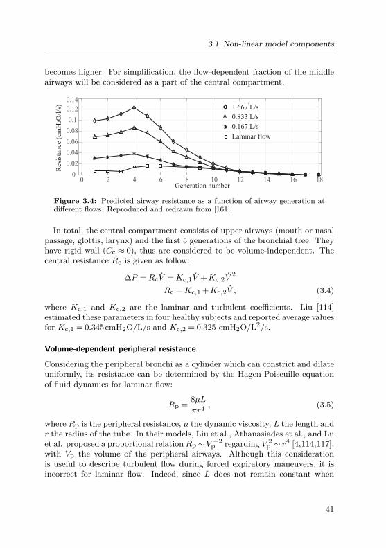
3.1 Non-linear model components
becomes higher. For simplification, the flow-dependent fraction of the middleairways will be considered as a part of the central compartment.
0 2 4 6 8 10 12 14 16 180
0.02
0.04
0.06
0.08
0.1
0.12
0.14
Generation number
1.667 L/s
0.167 L/s
0.833 L/s
Laminar flow
Resis
tance (
cm
HO
/l/s
)2
Figure 3.4: Predicted airway resistance as a function of airway generation atdifferent flows. Reproduced and redrawn from [161].
In total, the central compartment consists of upper airways (mouth or nasalpassage, glottis, larynx) and the first 5 generations of the bronchial tree. Theyhave rigid wall (Cc ≈ 0), thus are considered to be volume-independent. Thecentral resistance Rc is given as follow:
∆P =RcV =Kc,1V +Kc,2V2
Rc =Kc,1 +Kc,2V , (3.4)
where Kc,1 and Kc,2 are the laminar and turbulent coefficients. Liu [114]estimated these parameters in four healthy subjects and reported average valuesfor Kc,1 = 0.345cmH2O/L/s and Kc,2 = 0.325 cmH2O/L2/s.
Volume-dependent peripheral resistance
Considering the peripheral bronchi as a cylinder which can constrict and dilateuniformly, its resistance can be determined by the Hagen-Poiseuille equationof fluid dynamics for laminar flow:
Rp = 8µLπr4 , (3.5)
where Rp is the peripheral resistance, µ the dynamic viscosity, L the length andr the radius of the tube. In their models, Liu et al., Athanasiades et al., and Luet al. proposed a proportional relationRp∼V −2
p regarding V 2p ∼ r4 [4,114,117],
with Vp the volume of the peripheral airways. Although this considerationis useful to describe turbulent flow during forced expiratory maneuvers, it isincorrect for laminar flow. Indeed, since L does not remain constant when
41

3 Respiratory modeling
lung volume increases, Rp ∼ Lr−4 and Vb ∼ Lr2 occur, which leads to therelation Rp∼V −1
p . Widdicombe et al. derived a general term for the peripheralresistance [224]:
Rp =Kp,bVb
, (3.6)
whereKp,b [cmH2Os] is a positive constant and estimated to be 0.0014 cmH2O .minor 0.084 cmH2Os [224]. If the relation Valv/Vb ≈ const remains, eq. (3.6) canbe rewritten as:
Rp =Kp,bVb
= KpVlung
, (3.7)
whereKp is another positive constant. ForKp,b = 0.084cmH2Os and Vlung/Vb≈50 (Weibel), Kp can be estimated as Kp = 0.084 ·50 = 4.2cmH2Os.
Res
ista
nce R
Lung volumeTLCFRCRV
aw
Gaw
sGaw
Figure 3.5: Relationship between airway conduc-tanceGaw, specific airway conductanceGaw, airwayresistance Raw, and lung volume, as can be foundin literature. RV = residual volume. FRC = func-tional residual capacity. Redrawn from [94,98].
Briscoe and Dubois stud-ied the relation between to-tal airway resistance Rawand lung volume in 26 sub-jects of all ages [23] in-cluding 585 measurementswith a body plethysmograph.They found that Raw rangesfrom 2.9V −1
lung to 7.7V −1lung in
these subjects. They alsoreported a linear relationbetween airway conductionGaw = 1/Raw and lung vol-ume, which leads to the con-cept of a constant specificairway conductance, as intro-duced in Chapter 2:
Gaw = 1/Raw =KVlung, sGaw =Gaw/Vlung =K = const. (3.8)
The finding of Briscoe and Dubois (Fig. 3.5) is generally accepted and can befound in many textbooks of physiology.However, the subdivision of the airways into the central and peripheral com-
partment conflicts with the diagram in Fig. 3.5. The central compartment,especially the upper airways, consist of rigid tubes, and are therefore volume-independent. There is a need to investigate the exact contribution of the cen-tral compartment in the airway resistance-volume characteristics. Considering
42

3.1 Non-linear model components
eq. (3.4) and (3.7), the airway conductance Gaw can be rewritten as:
Gaw = 1Raw
= 1Rc +Rp
= 1Rc + Kp
Vlung
(3.9)
As a plausibility test, we reconstruct the data published by Bricose andDubois in one subject (named J.Z.) [23] and perform Least Squares regressionfor two mathematical models eq. (3.8) and (3.9). The results, illustrated in blueand red in Fig. 3.6, are K = 4.7899 with the squared 2-norm of the residual∑e2 = 0.642 in the original model and Rc = 0.1275, Kp = 4.4515, and
∑e2 =
0.6211 in the compartmentalized model. Similarly, the new conductance-volume curve differs slightly from the linear original one with a smaller residualerror (0.0746) against the original model (0.0936). The black lines in Fig. 3.6depict the resistance and conductance simulated with Rc = 0.345 (reportedin [4]) and Kp = 4.2 (as calculated above). Though the values come fromdifferent independent reports, its form and dimension fit the measured data(Fig. 3.6).
SimulatedFit with central compartmentOriginal fitMessured
Lung volume (L)Lung volume (L)
1.5 2 2.5 3 3.5 4 4.5 5 5.50.3
0.4
0.5
0.6
0.7
0.8
0.9
1
1.1
1.5 2 2.5 3 3.5 4 4.5 5 5.50.5
1
1.5
2
2.5
3
R(c
mH
O/L
/s)
2aw
G(
cmH
O)
2L
/saw
Figure 3.6: Resistance, conductance, and specific conductance against lung vol-ume. Least-squares regressions were performed for the original model of Briscoeand Dubois [23], and our model considering the central airway resistance.
This example demonstrates that the subdivision of airway resistance intoa volume-independent, central resistance and a volume-dependent, peripheralresistance is not only more physiological, but can also provide a better fit onexperimental data. Hence, the assumption of a linear relationship betweenGaw and Vlung should be replaced by the model shown in eq. (3.9), especiallyin cases of upper airway obstruction. More investigations on larger data shouldbe taken to confirm this hypothesis.
43

3 Respiratory modeling
Static pressure-volume relationship of the peripheral bronchi
In 1988, Gunst and Stropp [66] investigated the pressure-volume (PV) relation-ship measured in separated canine bronchi segments. This PV curve consistsof three phases: collapse, normal (linear), and over-distension (Fig.3.7). Sucha behavior can be modeled with a tangent hyperbolic (tanh) or a logarithmic(ln) function:
Vb = V0 + 1/λ · tanh(c ·Ptr,b +P0) (3.10)or Vb = 1/λ · ln(c ·Ptr,b +P0) +V0, (3.11)
where Vb is the bronchial volume and Ptr,b the transmural pressure. Theparameters V0, P0, c and λ can be used to adjust the form of the PV curve.
-20 -10 0 10 20 30-20
0
20
40
60
80
100
Volu
me
(% o
f m
axim
um
)
Transmural pressure (cmH O)2
Collapse
Linear
Over-distensiontanh function
Data
Figure 3.7: Pressure-volume relationship of theperipheral bronchi. Data taken from [66]
.
Figure 3.7 shows a fitof the tanh function tothe data from [66]. Thiscurve outlines the dependen-cies of the bronchial volumeon the pressure gradient be-tween the intra-thoracic andbronchial pressures. Duringthe collapsed and overexten-sion phases, a large changein the pressure gradient re-sults in a small change in thebronchial volume.
Model structureof airways and airspace
The model structure for airflow in the airways and airspace is illustrated in Fig. 3.8. Entering the periph-eral bronchi, the air flow is divided into two components: one passes throughthe bronchi and reaches the alveoli, and one expands the bronchi. The volumeand flow relations are given as:
Vlung(t) = Vc(t) +Vb(t) +Valv(t)→ Vlung(t) = Vb(t) + Valv(t) (3.12)Eq. (3.12) states a parallel structure between Vb and a series of Rp and Calv,which is known as the Mead’s parallel structure [128, 130]. The bronchi andalveoli compliances separate the material inside from the material outside.While air flow corresponds to the left side of the compliances (Cb and Calv)in Fig. 3.8, bronchi and alveoli are tethered to the surrounding interstitiumwhich, in our model, is assumed to be homogeneous for bronchi and alveoli.
44

3.1 Non-linear model components
Volume-dependentresistance
Flow-dependent resistance
Turbulent:
Laminar: const
Res
ista
nce
Com
pl.
(Vogel & Smidt )(Vogel & Smidt )
0
uawR C
Rp
cbR
C alv
b
lungV
C 0≈c
Upper airways + Central bronchi
Central airways AlveoliPeripheral bronchi
Mouth/nose
Interstitium
cR.
bV.
alvV.
L L
Figure 3.8: Model structure of airways and airspaces and their main compo-nents.
3.1.2 Tissue and chest wallThe respiratory system consists of three components: the gas (airways andairspace), the tissue enclosing the airways and airspace, and the chest wallenclosing the lungs (Fig 3.1). The change in volume of one part is equal tothat of the other parts [127]:
Vcw(t) = Vti(t) = Vlung(t) = Vb(t) + Valv(t). (3.13)
Eq. (3.13) indicates a serial structure among airways/airspace, tissue, and chestwall.
Separation of alveoli and interstitial tissue
One of the earliest investigation on the (quasi)-static relation of alveoli andinterstitial tissue was carried out by von Neergaard [214]. He compared expi-ratory pressure-volume curves of air-filled and liquid-filled lungs and empha-
45
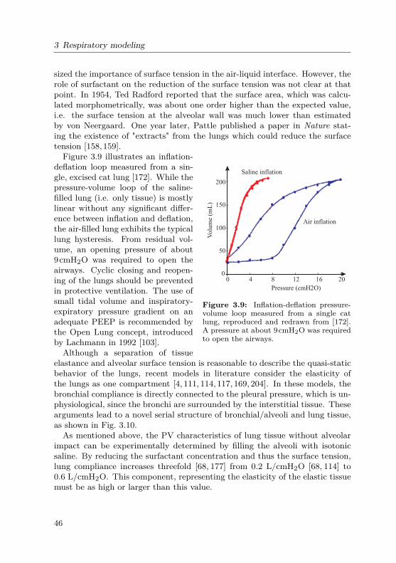
3 Respiratory modeling
sized the importance of surface tension in the air-liquid interface. However, therole of surfactant on the reduction of the surface tension was not clear at thatpoint. In 1954, Ted Radford reported that the surface area, which was calcu-lated morphometrically, was about one order higher than the expected value,i.e. the surface tension at the alveolar wall was much lower than estimatedby von Neergaard. One year later, Pattle published a paper in Nature stat-ing the existence of "extracts" from the lungs which could reduce the surfacetension [158,159].
0 4 8 12 16 200
50
100
150
200
Pressure (cmH2O)
Volu
me (
mL
)
Saline inflation
Air inflation
Figure 3.9: Inflation-deflation pressure-volume loop measured from a single catlung, reproduced and redrawn from [172].A pressure at about 9cmH2O was requiredto open the airways.
Figure 3.9 illustrates an inflation-deflation loop measured from a sin-gle, excised cat lung [172]. While thepressure-volume loop of the saline-filled lung (i.e. only tissue) is mostlylinear without any significant differ-ence between inflation and deflation,the air-filled lung exhibits the typicallung hysteresis. From residual vol-ume, an opening pressure of about9cmH2O was required to open theairways. Cyclic closing and reopen-ing of the lungs should be preventedin protective ventilation. The use ofsmall tidal volume and inspiratory-expiratory pressure gradient on anadequate PEEP is recommended bythe Open Lung concept, introducedby Lachmann in 1992 [103].Although a separation of tissue
elastance and alveolar surface tension is reasonable to describe the quasi-staticbehavior of the lungs, recent models in literature consider the elasticity ofthe lungs as one compartment [4, 111, 114, 117, 169, 204]. In these models, thebronchial compliance is directly connected to the pleural pressure, which is un-physiological, since the bronchi are surrounded by the interstitial tissue. Thesearguments lead to a novel serial structure of bronchial/alveoli and lung tissue,as shown in Fig. 3.10.As mentioned above, the PV characteristics of lung tissue without alveolar
impact can be experimentally determined by filling the alveoli with isotonicsaline. By reducing the surfactant concentration and thus the surface tension,lung compliance increases threefold [68, 177] from 0.2 L/cmH2O [68, 114] to0.6 L/cmH2O. This component, representing the elasticity of the elastic tissuemust be as high or larger than this value.
46

3.1 Non-linear model components
C
RpC alv
b Interstitium
R ti C tiCentral
Peripheral
Tissue Chest wall
R ti C ti
Figure 3.10: The serial structure airways/airspaces-tissue-chest wall.
Alveolar compliance
-20 -10 0 10 20 30 40 50
Pressure (cmH2O)
0
2
4
6
Vo
lum
e (
L)
alveoli
V = 0,5 Lmin
V = 5,6 Lmax
0,3 0,15
Figure 3.11: Pressure-volume characteristics ofthe alveoli [142].
Although the mechanical be-havior of alveoli surface ten-sion has been investigated bymultiple research groups [95,103, 140, 151, 201, 228], it isnot yet completely under-stood [27]. In their works,Yuta [228] and Sundaresanet al. [201] assumed that themain cause of lung volumechange during spontaneousbreathing is the recruitmentof alveoli, not the expansionof the opened alveoli. In ourapproach, the alveoli charac-teristics are considered as one non-linear component, which models the systembehavior of both recruiting and expending alveoli. The PV characteristics oflung alveoli can be described by the following hyperbolic function:
Valv(t) = V0 + 1λ· tanh(c ·Ptr,alv(t) +P0), (3.14)
where Valv(t) and Ptr,alv(t) are the alveolar volume and transmural pressure,respectively. The parameters V0, λ, c and P0 can be determined by maximumand minimum lung volume, as well as maximum alveoli compliance.Fig. 3.11 depicts the alveolar characteristics. The upper line represents the
alveolar compliance curve, and the lower one the compliance of diseased lungs,such as in edematous patients [32, 228]. The black circles in Fig. 3.11 illus-trate residual lung volume (RV = 1.3L [68]). The minimal volume of 0.5Lcorresponds to the state when the lungs are separated from the thorax and arecompletely collapsed. This approach does not yield any contradiction with theballoon-like theory or the recruitment model [228]. It should be noted that the
47

3 Respiratory modeling
alveolar hysteresis, as well as surface tension reduction regarding surfactant isnot in the focus of this work. A simplification is made by applying a tanh-function to describe the alveolar pressure-volume relationship. This can beextended in future works by replacing this characteristics with a more complexapproach, without affecting other model compartments such as tissue, airways,and chest wall.
Tissue and chest wall visco-elastic resistance
The total respiratory resistance can be divided into airway and visco-elastic re-sistances by means of measurements via body plethysmography and the forcedoscillation technique. The visco-elastic resistance, which accounts for less than43% of the total resistance [54], is a combination of lung and chest wall (in-cluding thoracic and abdominal) tissue damping. Ferris et al. performed mea-surements on test subjects using needles introduced to the trachea, the alveoli,and the pleural surface to separate these components of the resistance [51].They reported that the chest wall resistance, which is linear up to flow rates of2 L/s, accounts for 10−19% of the total resistance during nasal breathing andless than 19% during mouth breathing. They also found a low, insignificantpulmonary tissue resistance, as shown in Fig. 3.12. Hence, Rti ≈ 0 is consideredin our model.
0 0.5 1 1.5 2 2.5 3Pressure (cmH20)
0
1
0.5
2
1.5
Flo
w (
L/s
)
Chest wall
Nose
1
32 4
5
6
6
5
4
3
21 Tissue
Mouth
Pharynx-larynx
Lower airways
Figure 3.12: Flow-pressure relationship of respiratory segments, reproducedand redrawn from [51]. A high slope describes a low air flow resistance.
Lung-chest wall quasi-static interactions and the pleural space
In 1946, Rahn et al. introduced the pressure-volume diagram of the thoraxand the lung [173], as shown in Chapter 2. The chest wall compliance Ccw
48

3.2 The two-degree-of-freedom model
provides the elasticity of the components surrounding the lungs, i.e. thoraxand diaphragm. According to Athanasiades et al. [4], the non-linear pressure-volume curve of Ccw is sigmoidal and can be modeled by
Ptr,cw(t) = Acw−Bcw · log( TLC−RVVcw(t)−RV −0.999). (3.15)
The chest wall compliance Ccw is given as follow:
Ccw(t) = TLC−RVBcw
·exp(Acw−Ptr,cw(t)
Bcw)
[exp(Acw−Ptr,cw(t)Bcw
) +0.999]2. (3.16)
TLC is the total lung capacity, RV is the lung residual volume, Acw and Bcware constants. Applying parameters given in [4] will result in a maximum chestwall compliance of 0.3 L/cmH2O, which is comparable with the average valueof approx. 0.2 L/cmH2O given in literature [68,96,173].The parameter Acw from [4] causes a pressure drop over the chest wall Pcw =
0cmH2O and a pleural pressure Ppl = 0cmH2O at normal filling volume of thelungs. In normal condition of 3 L lung volume, a negative pleural pressurePpl ≈ −5cmH2O occurs [68]. In other words, the lungs are stretched and thechest wall is shrunk at FRC. Models which use two compliances in series needto be extended to present this negative pleural pressure. One solution is theintroduction of the extended pleural pressure source PPE, which incorporatesthe pre-stress of the chest walls and lung tissue. If PPE is set to 10cmH2O,the pressure gradient between chest wall and lung tissue will be around thisphysiological value [96]. This pleural-extended model succeeds in not onlypresenting the well-known PV characteristics of the chest (Fig. 3.14), but alsoa negative pleural pressure of Ppl ≈−5cmH2O.It should be noted that PPE does not present any physiological pressure
source within the pleural space, but rather the preload of lung and chest wallat FRC. Another, equivalent way to model the negative pleural pressure isto initialize the lungs and chest wall with a starting volume and modify thepressure-volume relationship with a shift in that volume.
3.2 The two-degree-of-freedom model
The degree of freedom (DOF) of a mechanical system is the number of in-dependent variables which are needed to describe that system entirely. Theconfiguration of the respiratory system as a series of the airways/airspace,the tissue, and the thorax can be expressed in terms of one single variable,the volume. In this consideration, the respiratory system has one DOF. The
49

3 Respiratory modeling
bronchial-alveolar parallel-structure gives the system another DOF. The over-all structure of the 2-DOF model is illustrated in Fig. 3.13. Rp,Cb,Calv, andCcw are non-linear components.The 2-DOF model is especially useful for simulating lung mechanics during
spontaneous breathing and mechanical ventilation, where the respiratory ratedoes not exceed 1 Hz (60 cycles per minute). High frequency components of therespiratory system such as inertance, upper shunt compliance (cheek vibration)are insignificant in this frequency range.
RcV
Pmouth
Pmus
Rp
Cb
R cwCalv Cti
C cw
Ppl
PPE
Figure 3.13: The two-degree-of-freedom lung model for low (physiological)frequencies. Rp,Cb,Calv, and Ccw are non-linear components.
3.2.1 Parametrization and implementationFor a healthy human during spontaneous breathing, parameter values may beobtained from literature by the following considerations:
• A constant central resistance Rc = 1cmH2OL−1 s is assumed, which isapproximately 25% of the airway resistance [68].
• The peripheral resistance Rp is given by eq. (3.7). The cumulative volumeof the peripheral airways is estimated to be about 50mL. At this volume,peripheral resistance is approx. 75% of the airway resistance [68].
• The pressure-volume characteristics of the bronchi and alveoli are givenin eq. (3.11) and eq. (3.14). Parameters are given in Tables 3.2 and 3.3.
• Lung tissue compliance is assumed to be constant Cti = 1L/cmH2O.
• The extended pleural pressure is modeled as constant PPE = 10cmH2O.
The total respiratory compliance is given as:1
Ctotal= 1
Clung+ 1Ccw
= 1Ctissue
+ 1Cb +Calv
+ 1Ccw
,
50

3.2 The two-degree-of-freedom model
Chest Pressure
1
-20 -10 0 10 20Pressure (cmH O)
1
1.5
2
2.5
3
3.5
4
4.5
5
5.5
Lung v
olu
me
(l)
12
3
2
chest wall
Figure 3.14: Implemented chest wall compliance according to [4]: (1) is theoriginal curve; (2) is the curve after adaption of Acw, and (3) after adaption ofPPE. Ppl is negative at lung volume < 4.25 L [142].
The maximum value of Ctotal is equal to 0.23 L/cmH2O in our model.
With the introduction of PPE, Acw needed to be adapted to achieve theoriginal chest compliance curve (Fig. 3.14). The parameters of the chest walland pleural space are given in Table 3.4.
Respiratory muscles
Consisting of the diaphragm and the intercostal muscles, the respiratory mus-cles provide the pressure gradient to inflate and deflate the lungs. In the pro-posed model, the pressure source is connected to the chest wall Ccw on one sideand to the atmosphere at the body surface on the other side. The alignmentof the pressure source in the circuit can be chosen corresponding to a negativeor positive Pmus. With the alignment shown in Fig. 3.13, Pmus becomes morenegative during inspiration, causing a fall in pleural pressure which drives airinto the alveoli and enlarge the thorax cavity. Since the pleural pressure Pplhas been shown to have an exponential form in healthy subjects [96], Pmus isalso likely to have an exponential form.
The implementation of Pmus is illustrated in Fig. 3.15. A periodic rectangu-lar pulse generator and a resistance-compliance (RC) network (Voigt model ofvisco-elastic behavior) is used to generate the signal.
51

3 Respiratory modeling
Table 3.2: Parameters of the collapsible airwaysResistance Compliance
Value Parameter ValueV1 0.05 V0 -0.0872R1 3 P0 7.4414
Vmin 0.005 λ 18.3776Popen 5
Table 3.3: Parameters of the alveoli compartment.Parameter Value UnitV0 3.05 Lλ 0.3922 L−1
c 0.1176 -P0 −0.8409 cmH2O
Table 3.4: Parameters of the chest wall and pleural space.Parameter Value UnitTLC 5.6 LRV 1.3 LAcw 7 cmH2OBcw 3.5 cmH2OPPE 10 cmH2O
3.2.2 Simulation results
Dynamic and static behaviors of the respiratory system
To demonstrate the behavior of the respiratory system during spontaneousbreathing, a simulation is performed with a respiratory rate of 0.2Hz (12breaths/min) and inspiration time of 2s. The amplitude of Pmus is set to5cmH2O. Figure 3.16 illustrates the simulative results including lung volume,alveolar, interstitium, and pleural pressure.During inspiration, pleural and alveolar pressures decreases below Patm, so
that air enters the lungs and loads the compliances. At the end-inspiratoryphase, minimal pressures occurs equal to Pint =−7.1 cmH2O in the interstitiumand Ppl = −8.3 cmH2O in the pleural space. FRC is 2.5 L, and tidal volume
52

3.2 The two-degree-of-freedom model
5 10 15 20
Time (s)
-5
-4
-3
-2
-1
0pre
sssu
re (
cmH
2O
)
5 10 15 20
time (s)
-5
-4
-3
-2
-1
0+
-
+
-
P (t)
2s
3s1 Ohm
0.7 Farad
+
-
Pre
ssure
(cm
H2O
)
mus
Figure 3.15: The respiratory muscles Pmus during spontaneous breathing,generated by a pulse generator and a RC network [142].
40 41 42 43 44 45 46 47
Time (s)
-10
-8
-6
-4
-2
0
Pre
ssure
(cm
H2O
)
2.5
2.75
3
Volu
me
(L)
0
-2
-4
-6
-8
0
0.25
0.5
Pre
ssu
re (
cmH
2O
)
alveolar pressure
interstitial pressure
pleural pressure
lung volumelung volume change (l)
alveolar pressure
pleural pressure
1 2
Figure 3.16: Respiratory pressures and volumes during spontaneous breath-ing [142]. (1): Literature values, reproduced from [68], (2) Simulation resultswith a functional residual capacity of 2.5L.
VT is 500 mL. At end-expiration (t≈ 45 s), the pleural pressure is Ppl =−5.74cmH2O, the interstitial pressure Pint =−4.94 cmH2O, and the alveolar pressureis slightly positive Palv = 0.015 cmH2O. All values and dynamics describedin [68] can be simulated successfully.
53

3 Respiratory modeling
Static pressure-volume relationship during mechanical ventilation
During mechanical ventilation, the monitoring of lung mechanics via PV char-acteristics is important, since lung over-stretching can occur if airway pressureexceeds 30cmH2O [17]. For simulation purposes, a model of the mechani-cal ventilator is constructed, which can provide pressure-controlled or volume-controlled ventilation modes. Incremental increases of PEEP and PIP areapplied to investigate the dynamic response of lung mechanics to PEEP. Therespiratory muscles are deactivated as soon as mechanical ventilation starts.The total respiratory compliance Ctotal was calculated as the quotient of thetidal volume VT and the overall pressure drop [111]:
Ctotal = VTPIP−PEEP . (3.17)
Analogously, lung compliance is the quotient of VT and the pressure drop overthe lung, which was measured continuously during the simulation.Figure 3.17, top three diagrams present the results including alveolar and
pleural pressure, lung volume, and lung and total compliance. Fig. 3.17, bottompanel presents the simulated static PV characteristics of lungs and chest wallcompared to literature data reconstructed from [96]. At FRC, the pressureof lungs and thorax are opposite and equal, which results in a zero overallpressure.Ppl becomes positive at high ventilation pressures Pven > 15cmH2O. Total
compliance decreases from 0.124 L/cmH2O at PEEP= 0 to 0.03 L/cmH2O atPEEP= 25 cmH2O due to the implementation of non-linear compartments. Asa result of this stiffness change, tidal volume falls from 1.241 L (PEEP=0) to0.272 L (PEEP=25). The mean pressure and volume of each PEEP setting fitexactly in the static PV-relationship of lung and thorax. The operating pointof the system moves upwards from A (PEEP=0) to F (PEEP=25) regardingthe increasing PEEP. Simulation results demonstrate the ability of the modelto quantify the non-linear change in tidal volume and compliance during aPEEP-trial.
3.2.3 The linearized respiratory modelLinearization and parametrization
Applying the model for spontaneous breathing with normal tidal volume, thenon-linear behavior in pressure-volume or pressure-flow relationships can bereplaced by linear resistances and compliances. The result of this process is thelinearized model. For simplification, we keep the same notation for the linearmodel as used in the non-linear one. In high dynamic measurement techniques
54

3.2 The two-degree-of-freedom model
chest
FRCFRC
2
6
4
resting chest
residual volume
lung v
olu
me (
L)
chest wall
1
21
-100
102030
(cm
H2O
)alveolar
pleural
pressures
2
4
6
(L) lungs
total
volumes
time (s)
0
0.1
0.2
(L/
cmH
2O
)
lungs
total
compliances
PEEP
-15 20 401
2
3
4
5
lung v
olu
me
(L)
PV-relationship
PIP
Transmural pressure (cmH2O)0
2520
0
15
10
5
BA
E
CD
F
A
B
C
D
EF
PEEP
Transmural pressure (cmH2O)
Ppl PalvPtm
-40 200 40-20
lungs
180 210
20 40
15090 1206030
Figure 3.17: Top three diagrams: ventilation pressures, lung volumes andcompliance during a PEEP trial. PEEP was incrementally increased from 0to 25cmH2O, PIP was set equal to PEEP +10cmH2O. Bottom graph: Staticpressure-volume loop of lung and chest wall. (1): Literature values, reproducedfrom [96], (2): Simulation results. A-F mark the operating points of the systemfor each set of PEEP and PIP [142].
such as interrupter or forced oscillation technique, the system inertance I andupper airway compliance (cheek vibration) Cmouth need to be considered. Thenew linear model is illustrated in Fig. 3.18.Typical parameter values of the linear model are:
• Ccw = 0.3; Rcw = 1
55

3 Respiratory modeling
RcV
Pao
Pmus
Rp
Cb
RcwCalv Cti Ccw
Ppl
Cmouth
IVlungao
Vb
Valv
Pint
Palv Vlung
Patm
Figure 3.18: The linear lung model with inertance and upper shunt compliance.
• Cti = 1; Calv = 0.2; Cb = 0.004
• Rp = 2; Rc = 0.15; I = 0.01.
• Cmouth is between 0.0001667 (cheek supported and 0.001 (cheek unsup-ported)).
• The overall resistance and compliance of the system are
Rrs = Rc +Rc +Rcw = 0.35Clung = (Calv +Cb)||Cti = 0.1667 (3.18)Crs = Clung||Cchest = 0.1
Resistances, inertance, and compliances are given in cmH2O/L/s, cmH2O/L/s2,and L/cmH2O, respectively. Values are taken by linearizing the non-linearmodel as well as from literature [10,210].
Alteration of model parameters under pathological conditions
Model parameters alter under pathological conditions. The following alter-ations, which correspond to clinically relevant diagnoses, are of interest [210]:
• Central obstruction: increase in central resistance Rc = 5 (grade 1); Rc =10 (grade 2).
• Peripheral obstruction: increase in peripheral resistance, main cause ofasthma and COPD, Rp = 5 (grade 1); Rp = 10 (grade 2).
• Pulmonary restriction: reduction of alveolar or tissue compliance Calv =0.02; Cti = 0.01.
• Thoracic restriction: reduction of thoracic compliance Ccw = 0.03.
56

3.3 Model-based analysis of the interrupter technique
• Bronchial sclerosis: decrease in bronchial compliance Cb = 0.002−0.008.
• Non-obstructive emphysema (over-extension): increase in Calv and de-crease in Cb; Calv/Cb 50.
• Obstructive emphysema (non-obstructive emphysema and obstruction):Calv/Cb 50 and Rp = 5.
Resistances, inertance, and compliances are given in cmH2O/L/s, cmH2O/L/s2,and L/cmH2O, respectively.
3.3 Model application: analysis of the interrupter technique
This section analyses the behavior of the respiratory system in the time do-main aiming to reevaluate the interrupter technique. As introduced in sec-tion 2.2, this technique provides the resistance based on the assumption thatthe pressure at airway opening Pao equilibrates the alveolar pressure Palv di-rectly after an occlusion. According to Marshall and Dubois [123], the inter-rupter method measures the total resistance of the whole respiratory system,including airways, lungs, and chest wall. In the original researches of Batesand Sly [10,12,14,18,188], which are the basics of the ATS/ERS official state-ment [19], the authors introduced a computer model of two compartments usingthe Otis parallel structure. By setting inhomogeneous airway resistances foreach lung (R1 = 3R2), they suggested that the pendelluft between two lungs isthe main cause of the second rise in Pao after an occlusion. Since these modelscontain only airways without any consideration of lung tissue, chest wall, andrespiratory muscles, their explanation on Pdiff seems to be incomplete.In fact, there is another, widely accepted opinion, that the second rise in
Pao is caused by the respiratory muscles [163]. During the occlusion, thesemuscles continue their activities, since the duration is short enough not tocause any nervous response. Hence, the interrupter technique is also usedin mechanical ventilation to measure the pressure generated by respiratorymuscles in ventilated patients [115, 116, 163]. The airway occlusion pressureP0.1 measured during the first 100 ms after the occlusion has been reported toplay an important role in patient weaning [85,180].In this section, we extend our 2-DOF model to describe the system dynamics
during interrupter measurements. The aim of this section is to clarify the roleof the respiratory muscles and the pendelluft phenomenon in the second risein Pao.
57

3 Respiratory modeling
3.3.1 Model behavior during an interruptionThe equations of motion of the linear system (Fig. 3.18) are given as:
Pmus(t)−Pao(t) = Ptr,cw(t) +RcwVlung(t) +Ptr,ti(t) +Ptr,alv(t) ++RpValv(t) +RcVlung(t) + IVlung(t) (3.19)
Ptr,b(t) = Ptr,alv(t) + Valv(t)Rp (3.20)Ptr,mouth(t) = Pao(t). (3.21)
Ptr,b and Ptr,mouth are the transmural pressure over the compliance Cb andCmouth.Let ts be the closing time, t−s the moment shortly before and t+s the mo-
ment shortly after closing. The pressures over compliances and the respiratorymuscles do not change during the closing process, i.e.:
Pmus(t−s ) = Pmus(t+s )Ptr,cw(t−s ) = Ptr,cw(t+s )Ptr,ti(t−s ) = Ptr,ti(t+s )Ptr,alv(t−s ) = Ptr,alv(t+s ). (3.22)
Applying eq. (3.19) for t = t−s and t = t+s and subtracting them from eachother leads to:
Pao(t−s )−Pao(t+s ) = (Rcw +Rc)(Vlung(t+s )− Vlung(t−s )) ++Rp(Valv(t+s )− Valv(t−s ) + I(d(Vlung(t+s )− Vlung(t−s ))/dt) (3.23)
Let ∆Pao = Pao(t−s )−Pao(t+s ) and ∆Vlung = Vlung(t+s )− Vlung(t−s ) be theflow and pressure gradients before and after the closing of the interrupter. Thebronchial volume Vb is small compared to that of the lung Vlung (eq. (3.3) andeq. (3.1)), i.e. the alveolar and total volume can be considered to be equal:Valv = Vlung− Vb ≈ Vlung. Eq. (3.23) becomes:
∆Pao = (Rc +Rp +Rcw)∆Valv + I(d(∆Valv)/dt) (3.24)
The first term describes the resistive behavior between the pressure andflow drops before and after an occlusion. The second term I(d(∆Vlung,s)/dt)corresponds to a Dirac-impulse in ∆Pao,s at t = ts caused by the inertanceI. Neglecting the second term and considering that the flow at the airwayopening becomes zero directly after shutting (perfect valve closing, Valv(t−s ) =0, ∆Valv = Valv(t+s )), eq. (3.24) becomes:
∆Pao = (Rc +Rp +Rcw)Valv(t+s ) = (Rc +Rp +Rcw)Vao(t+s ). (3.25)
58
3.3 Model-based analysis of the interrupter technique
Comparing eq. (3.25) with eq. (2.11) shown in Chapter 2:
Rint = ∆PaoVao
,
the relationship of the interrupter resistance Rint and other resistance com-ponents can be derived as:
Rint =Rc +Rp +Rcw (3.26)Eq. (3.24) shows that the interrupter resistance, calculated by the quotient
of the pressure gradient over flow drop immediately before and after closing ofthe interrupter, is the sum of airway resistance and chest wall tissue resistance.The chest wall component Rcw includes approx. 30-40% of the total resistance,thus contributes a significant fraction to the total resistance. During bronchialchallenge or bronchodilator test, the chest wall component is less affected thanthe airway resistance. This explains why Rint is less sensitive than the spe-cific airway resistance sRaw measured with the body plethysmography duringdiagnostics of airway obstruction, since sRaw contains only airway resistancewithout any visco-elastic damping components [97]. We should keep this pointin mind when performing the interrupter technique.To analyze the cause of the second rise in ∆Pao,s, a random time instant t
between closing and reopening ts < t < tr is considered. During this period, allflows in the system remain zero (∆Vlung = ∆Valv = 0), thus eq. (3.19) becomes
Pmus(t)−Pao(t) = Ptr,cw(t) +Ptr,ti(t) +Ptr,alv(t) (3.27)Since all flows are zero, the volume of the chest wall, tissue, airway and airspacecompartments remain unchanged, and so do the transmural pressures Ptr,cw,Ptr,ti, and Ptr,alv, i.e.:
Pmus(t)−Pao(t) = const for ts < t < tr (3.28)Eq. (3.28) indicates that the second rise in Pao(t) is equal to the change inPmus(t) during the closing period. This shows that the respiratory musclesplay a mayor role in the second rise and can not be ignored in the model, asreferenced in the ATS/ERS document [10,188].
3.3.2 Simulation-based analysis of the interrupter techniqueEq. (3.24) and (3.26) present the mathematical background of the ideal inter-rupter technique. In real measurements, several disturbing factors caused bythe system inertance, the imperfect closing process of the shutter, the upperairway (cheek) compliance, the bronchial compliance, and the pendelluft be-tween left and right lung occur. Matlab Simscape™ provides a sophisticatedtool to investigate the influences of these disturbances.
59

3 Respiratory modeling
Effect of the respiratory muscles
First, we demonstrate an ideal interruption, in which the inertance, mouthand bronchial compliances are set to zero. An interruption during inspirationis realized at t= ts = 17.4 s for 0.2 s by an ideal switch-element in Simscape™ .The closing and releasing processes are also assumed to be ideal. Simulationresults for spontaneous breathing are shown in Fig. 3.19. In the left graphic,Pmus is set to normal spontaneous breathing pressure as shown in Section 3.2.In the right graphic, Pmus remains constant while the shutter is closed. Thisholding corresponds to the Hering-Breuer Inflation Reflex in infants and youngchildren (see Section 2.2.4). Note that in infants, an expiration starts directlyafter a HBIR inspiratory pause, which is not considered in the simulation.In the left graphic, flow and pressure change abruptly after closing the valve
at t = 17.4 s. The pressure exhibits two rises: one jump direct at the momentof closing and one ramp between 17.4 s and 17.6 s. As a contrast, the rightgraphic, simulating a constant Pmus during interruption, does not exhibit anyramp in Pao after the first jump. This pressure remains unchanged for constantPmus.
16.5 17 17.5 18
Time (s)
-6
-4
-2
0
2
cmH
2O
an
dL
/s Vao
Pao
Pmus
16.5 17 17.5 18
Time (s)
-6
-4
-2
0
2
cmH
2O
an
dL
/s Vao
Pao
Pmus
P = constmus
ΔPao
˙ΔVao
first risesecond rise
first rise
Hering-Beurer
Figure 3.19: Flow and pressure at airway opening, as well as respiratory mus-cles Pmus during an ideal interrupter. Shutter is closed at 17.4 s and released at17.6 s. Left: normal Pmus. Right: Pmus is hold as constant while the shutter isclosed.
The interrupter (total) resistance can be computed as the ratio ∆Pao/∆Vaomarked in the left graphic. The simulation results demonstrate that the secondrise in Pao is directly related to the change in the respiratory muscles Pmus.While the first rise is believed to related to the airway resistance and the secondrise to the tissue resistance in some literatures, as reviewed in [101], our model-based analysis and simulation results strongly support another physiologicalexplanation: the interrupter resistance, which causes the first rise, consists of
60

3.3 Model-based analysis of the interrupter technique
airways and tissue/chest wall damping, while the second rise is caused primarilyby the respiratory muscles.
Effect of disturbances
Pressure and flow measured at airway opening are affected by several distur-bance factors: inertance, bronchial and upper airways, and imperfect valveclosing. These effects can be demonstrated by adding disturbing componentsto the model. The simulation results are depicted in Fig. 3.20.
• Figure 3.20 (A) presents the effect of the inertance I (eq.(3.24)) as aDirac-impulse, appearing directly after valve closing.
• The effect of the bronchial compliance Cb can be analyzed considering Vb> 0 (compared to eq. (3.23)). This models the distention of the bronchiright after closing the valve. A charging process occurs between alveolarand bronchial compartments right after closing the valve with the timeconstant τb given as:
τb =Rp ·Cb ·CalvCb +Calv
(3.29)
τb has a typical value at 2 · 0.20.0040.204 = 0.0078 s. This value is ten times
smaller than the normal duration of an interruption (100 ms). Figure 3.20(B) displays the charging process caused by Cb. The small time constantmakes this disturbance relatively insignificant to the measurement.
• Similar to the bronchi, the upper airway (cheek) is also distended duringthe valve closing process. Its time constant is related to resistances andcompliances of the entire system Cmouth:
τmouth = (Rc +Rp +Rcw) · 11Ccw
+ 1Cti
+ 1Calv
+ 1Cmouth
.
≈ Rint ·Cmouth, since Cmouth Calv,Cti,Ccw(3.30)
The typical value of τmouth is estimated to be around 3.1 ms for smallCmouth = 0.001 (with supported cheek) and 28.6 ms for large Cmouth =0.01 (without supported cheek). Although a small cheek compliance isinsignificant for the measurement of pressure, as shown in Fig. 3.20 (C),an unsupported cheek can cause a delay in the result, as displayed inFig. 3.20 (D). In contrast to the bronchi, the effect of the cheek compli-ance on the results can vary among measurements due to the executionof the test and the cooperation of the patient.
61

3 Respiratory modeling
0
0.5
1
cmH
2O
an
dL
/s)
Vao
Pao
0
2
4
6
8Vao
Pao
Time (s)
0
0.5
1
cmH
2O
an
dL
/s)
Vao
Pao
0
0.5
1
cmH
2O
an
dL
/s)
Vao
Pao
0
0.5
1
1.5Vao
Pao
17.2 17.4 17.6 17.8-0.5
0
0.5
1
1.5
2
cmH
2O
an
dL
/s)
Vao
Pao
17.2 17.4 17.6 17.8
0
0.5
1
1.5
2Vao
Pao
0
0.5
1 Vao
Pao
Time (s)
(B): C = 0.004b
(A): I = 0.01
(C): C = 0.001m
(D): C = 0.01m
(E): Imperfect valve closing (F): combination of (A-C) and (E)
(G): (F) with normal Pmus (H): (G) with 0.00017C =m
first rise
second rise
first rise
second rise
Figure 3.20: Simulated flow and pressure demonstrating the effect of differentdisturbances in the interrupter technique. (A-F) Holding of Pmus during inter-ruption duration. (G-H) normal Pmus. (A) Bronchial compliance Cb = 0.004.(B) Inertance I = 0.01. (C) Mouth compliance Cmouth = 0.001. (D) Mouthcompliance Cmouth = 0.01. (E) Imperfect closing of the valve. (F): combinationof (A-C) and (E). (G): (F) with Pmus. (H): (G) with Cm = 0.00017.
62

3.3 Model-based analysis of the interrupter technique
• The shutting of a valve is a dynamic process on it own, which dependson the construction and manufacturing of the valve. To demonstratethe effect of the valve on the measurement, we replace the ideal switchby a conductance that falls linearly from 103 to 10−10 within 15 ms, asreported in [10]. The result is illustrated in Fig. 3.20 (E). The 12 msperiod can be observed in the simulated flow and pressure, which doesnot exhibit a typical exponential charging curve. Its form depends on thechange of the conductance (or resistance) during the valve closing. Theopening of the valve is demonstrated as ideal without any delay.
• The combination of all introduced disturbances are displayed in Fig. 3.20(F), (G), and (H). In Fig. 3.20 (G) and (H), the respiratory muscles arereactivated. All pressure responses exhibit dynamic behavior which canbe observed in literature [65, 101]. The plotted curve has the form of aDT2 response describing a system consisting of one inertance and twocompliances.
3.3.3 Pendelluft and the Otis parallel model structureThe Otis-parallel structure is based on the consideration of the lungs as a bi-furcation of two RC-pathways connected in parallel [157]. This representationof the lungs, referred to as the "bifurcation model", focuses on the pulmonarycompartment differences to explain the frequency behavior of the parametersand even the asynchronous ventilation between the lungs [157]. Bates andSly [10, 188] applied this model to the interrupter technique and proposed theeffect of pendelluft1 as the main reason for the second rise in airway pres-sure. However, they did not consider the influence of the chest wall and therespiratory muscles.We extend our linear model by the Otis-parallel structure to the model shown
in Fig. 3.21. The model has two branches, each one consists of one resistanceand one compliance. During the interruption period, if there is a pressuregradient between the two compliance C1 and C2, there will be a redistributionprocess of air between the two compartments with the time constant τpendel:
τpendel = (R1 +R2) · C1 ·C2C1 +C2
(3.31)
Let R1 = 1,R2 = 3cmH2O/L/s and C1 = C2 = 0.05L/cmH2O as used in [10],τpendel can be calculated to (1+3) · (0.05∗0.05)/0.1 = 0.1s. This time is large
1The German word "Pendelluft" refers to the movement of air back and forth betweenthe lungs. It is thought to increase the respiratory dead zone and cause ventilationinhomogeneity between the lungs.
63

3 Respiratory modeling
RcV
Pao
Pmus
R1 RcwC1 Cti Ccw
Ppl
Cmouth
IVlungao V1
Pint
Vlung
Patm
R2C2
V1
Figure 3.21: The linear lung model with the Otis-parallel structure.
enough to have an influence on the pressure change during the interruptiontime, as illustrated in Fig. 3.22 (I). If the resistance distribution is inhomoge-neous, but the time constants are equal, for example R1 = 1,R2 = 3cmH2O/L/sand C1 = 0.075,C2 = 0.025L/cmH2O; τ1 = τ2 = 75ms, the second rise causedby the pendelluft disappears (simulation 3.22 (J)).Adding I, Cmouth, and Pmus to the model results in more realistic simulation
results (Fig. 3.22 (K) and (L)). It is obvious that the impact from Pmus is likelydominant in the second rise in Pao. It should be noted that the inhomogeneityof R1/R2 = 1 : 3 has previously been assumed by the group of Bates [14, 188],which may corresponds to a severe obstruction. In healthy adults, no signif-icant inhomogeneity is expected (typical values are 53% to 47%, as reportedin [186]). Since the second rise in Pao can always be observed in measurementswith the interrupter technique, even in healthy subjects, we do not supportthe idea of the pendelluft as the main cause of the second rise as mentionedin the ATS/ERS document [19]. In future works, the effects of the pendelluftduring the interrupter technique should be further reevaluated in larger stud-ies, possibly in combination with the Electrical Impedance Tomography (seeChapter 6).
3.4 Summary
This chapter presents a novel biophysical (forward) model of respiratory me-chanics. Following the object-oriented compartment modeling, we subdividedthe system into upper and central airways, peripheral (bronchial) airways, tis-sue, pleura and chest wall. The model considers significant non-linearities ofmodel components. Simulation results demonstrate the high performance ofmodel responses compared to data from literature. The model can be used tomonitor the change of the compliance during mechanical ventilation.Analyzing respiratory mechanics during spontaneous breathing, model lin-
earization should be applied for simplification. We investigate the system re-sponses of the linear model to reevaluate physiological interpretation of the
64

3.4 Summary
(I): R =1, R = 3, C = C = 0.051 212
(J): R =1, R = 3,C = 0.075, C = 0.0251
1
2
2
0
0.5
1
17.2 17.4 17.6 17.8
0
0.5
1
17.2 17.4 17.6 17.80
0.4
0.4
0.8
cmH
2O
)
Vao
Pao
(K): (I) with I and C mouth (L): (K) with P mus
Pmus
Pendelluft
0
Flo
w (
L/s
)
0
0.8
Pre
ssure
(
17.2 17.4 17.6 17.80
0.4
0.4
0.8
cmH
2O
)
Vao
Pao
0
Flo
w (
L/s
)
0
0.8
Pre
ssure
(
Vao
0
0.5
1
Pao
Time (s)
17.2 17.4 17.6 17.8
0
0.5
1
1.5
Time (s)
cmH
2O
)F
low
(L
/s)
Pre
ssure
( cmH
2O
)F
low
(L
/s)
Pre
ssure
(
Vao
Pao
Figure 3.22: Simulated flow and pressure demonstrating the effect of the pen-delluft in the interrupter technique. (I-K) Holding of Pmus during interruptionduration. (I) different time constants between two compartments. (J) same timeconstants in both compartment. (K) I with inertance and cheek compliance. (L)I with Pmus.
interrupter technique. The interrupter resistance Rint is composed by the air-ways and visco-elastic (tissue and chest-wall) resistances. The second rise inPao is mainly caused by the respiratory muscles Pmus in adults and children.There is a need for a deeper investigation on effects of the pendelluft duringthe tests.
65


4 Model-based parameter estimation with the forcedoscillation technique (FOT)
Look at situations from all angels,and you will become more open.
Dalai Lama XIV
This chapter focuses on the dynamic response of the respiratory system inthe frequency domain. As introduced in Chapter 2.2, the forced oscillationtechnique (FOT) measures the respiratory impedance Z(jω) over a range offrequencies. Although FOT has a high potential use in infants, young children,and sleeping patients, clinical use of FOT is still limited. Medical workersusually have trouble interpreting the real and imaginary part of the compleximpedance Z(jω). Moreover, current physiological interpretation of Z(jω) bymeans of different modeling approaches is controversial, even in the ATS/ERSguidelines [19].First, this chapter presents a FOT measurement system and the computation
of Z(jω) in the frequency domain. Second, a discussion on the limitation ofthe existing models will be given, followed by new approaches and hypothesesfor parameter estimation using FOT. Third, the chapter discusses the use ofFOT in combination with nasal masks.
4.1 Measurement of respiratory impedance
The FOT device used in this research is the Philips Respironics CoughAssistE70 (Philips, Eindhoven, The Netherlands). The function of this device isbased on the generation of high frequency oscillations superimposed on a pos-itive pressure, then rapidly shifting to a negative pressure to generate a highexpiratory flow rate for secretion clearance. In combination with a pneumota-chograph, the CoughAssist functions as a FOT device that generates sinusoidalvibrations. During our FOT measurements on volunteers, the device appliedoscillation at an amplitude of 4cmH2O and frequencies between 3 and 20Hzsuperimposed on a positive baseline pressure at 4cmH2O. Test subjects wereconnected to the FOT device through a tube, a bacteria filter, and a mouthpiece.Flow and pressure were recorded at the subject’s airway opening with a Hans
Rudolph linear Fleisch pneumotachometer (Hans Rudolph, Kansas, USA) at1 kHz sampling rate. The sensor was heated to 37C to prevent condensationon the internal mesh. The signals were sent to a Hans Rudolph PneumotachAmplifier Series 1110 (Hans Rudolph, Kansas, USA) and converted into ana-
67

4 Model-based parameter estimation with the forced oscillation technique (FOT)
logue voltage signals. A National Instruments USB.X Series MultifunctionDAQ (National Instrument, Texas, USA) was used to capture data at 1kHzsampling rate. Data analysis is performed in MATLAB 2015b (The MathWorksInc., Natick, Massachusetts, USA).
Data analysis in the frequency domain
The calculation of the respiratory impedance Z(jω) is performed in the fre-quency domain. A second-order Butterworth IIR filter with a bandwidth of0.2Hz and the center frequency equal to the oscillation frequency is appliedon Pao(t) and Vao(t) to separate the oscillation from the spontaneous breath-ing (Fig. 4.1). To achieve a zero phase shift, the filter is applied forward andbackward over the data.
5 6 7 8 9 10
Frequency (Hz)
-40
-20
0
Mag
nit
ud
e(d
B)
0 5 10 15 20 25Frequency (Hz)
0
0.2
0.4
0.6
0.8
|Flo
w|
(L/s
)Original
After bandpassfiltering
Figure 4.1: Left: Amplitude of the frequency response of the Butterworth-bandpass filter second order, fos = 7Hz. Right: fast Fourier transform of theflow amplitude before and after applying the bandpass filtering.
The calculation of Z(jω) is possible via two methods: the fast Fourier trans-form (FFT) and the windowed cosine fitting (WCF).
Fast Fourier transform
The fast Fourier transform (FFT) splits a signal into a sum of cosine wavesof different frequencies, amplitudes, and phases. Considering one oscillationfrequency ω = ωos, the amplitude and phase of Z(jωos) can be determined bythe amplitude and phase of the fast Fourier transformed pressure and flow atω = ωos:
|Z(jω)|ω=ωos = |P (jωos)||V (jωos)|
(4.1)
ϕ(jω)|ω=ωos = ϕP (jωos)−ϕV (jωos). (4.2)
68

4.1 Measurement of respiratory impedance
The complex impedance of the bacteria filter was measured separately andsubtracted from Z(jω) to achieve accurate values for respiratory impedance.Alternatively, Z(jω) can be calculated by the mean Fourier crossspectrum
SPV and autosprectrum SV V of the pressure and flow signals:
Z(jω)|ω=ωos =SPV (jω)SV V (jω) |ω=ωos (4.3)
Cosine and windowed cosine fitting:
The bandpass-filtered flow and pressure signals comprise only one frequencycomponent:
P (t) = AP · cos(ωt+φP )V (t) = AV · cos(ωt+φV ),
where A, φ are amplitude and phase, respectively. Fitting the data with thesecosine functions at each oscillation frequency ωos results in amplitude and phaseof Z(jω).
Cosine fitting : (4.4)
ZR(ωos) = ReZ(jωos)= APAV· cos(ϕP −ϕV )|ω=ωos
ZX(ωos) = ImZ(jωos)= APAV· sin(ϕP −ϕV )|ω=ωos
Performing the cosine fitting for a finite-length window with N data samplesof P (t) and V (t) and sliding that window over the whole measurement dura-tion, Z(jω) can be computed as an function of time [91]. For each N samplesof the current sliding window, the amplitudes and phases AP , AV , φP and φVare determined by applying Least-Squares fitting. The computed impedanceis considered to be the value at the middle position of the window (N/2).
Windowed cosine fitting : (4.5)ZR(ωos, tN +N/2) = AP /AV · cos(φP −φV )|ω=ωos
ZX(ωos, tN +N/2) = AP /AV ·sin(φP −φV )|ω=ωos ,
where tN is the start position of the window.An exemplary window size of 0.4s gives N a value of 400 at 1 Hz sampling
rate. The WCF method is a combination of the time and frequency domains.
69

4 Model-based parameter estimation with the forced oscillation technique (FOT)
1.5
2.5
1.0
-1.0
0.5
0.0
-0.5
-1.53 5 6 7
Frequency (Hz)201510R
esis
tance
(cm
HO
/L/s
)2
|Z |
Rea
ctan
ce |Z
| (
cmH
O/L
/s)
2
8 9 12 3 5 6 7Frequency (Hz)
2015108 9 12
2.0
3.2
3.6
3.0
2.8
2.6
3.4
2.4
Fast Fourier transform
Windowed cosine fitting
Cosine fitting
Windowed cosine fitting
Fast Fourier transform
Cosine fitting
XR
Figure 4.2: Representative resistance and reactance measured on one healthysubject. Calculation of Z(jω) with three different methods: fast Fourier trans-form, cosine fitting and windowed cosine fitting.
Results
Fig. 4.2 shows representative data of the respiratory impedance from one testsubject. The resulting reactance shows a positive trend with a resonance fre-quency at about 7Hz. The resistance shows a negative frequency gradient from3.4 to 2.6cmH2O/L/s. The different methods provide almost the same valuesfor resistance and reactance.
4.2 Modeling and parameter identification
4.2.1 A survey of lung models used in Forced Oscillation Technique
A physiological interpretation of Z(jω) can be made in combination with math-ematical (greybox)-modeling and parameter estimation. The simplest model ofthe respiratory system in oscillometry is the serial RIC-network (Fig. 4.3(F)).The inertance, which can be neglected for respiratory frequencies under 2Hz asin spontaneous breathing and mechanical ventilation, contributes a significantpart to Z(jω) at higher frequencies:
ZRIC(jω) =R+ jωI+ 1jωC
. (4.6)
The extended-RIC model (Fig. 4.3(G)) has a peripheral resistance Rp addedin parallel to the compliance C to fit the frequency-dependency of the impedance’sreal part to experimental data [9, 39, 84, 145]. Physiologically, Rp is thoughtto correspond partially to the airway resistance of the proximal airways. C isthought to be lung compliance [39, 84], Rc the central resistance, and I theinertance. However, this common interpretation of C seems to be incorrect
70

4.2 Modeling and parameter identification
and will be discussed later in this chapter. The total impedance of the modelis given as:
ZeRIC(jω) =R+ Rp1 +(ωRpC)2 + j
(ωI−
ωR2pC
1 +(wRpC)2
)(4.7)
R I C
cR I
C
R
eC
cR I
C
Rp
p
(F): RIC
(H): augmented RIC
(G): extended RIC
p
R I
C
R
b
C
C
e
cw
Cl
(I): Mead
c
Figure 4.3: Lung models in oscil-lometry. c = central, p = periph-eral, b = bronchial, aw = airway,cw = chest wall, s = static, ve =visco-elastic, e = extra-thoracic, t= tissue, g = gas.
The augmented-RIC model (Fig. 4.3(H))is an extension of the extended-RIC modelcomplemented by the extrathoracic compli-ance Ce. This component presents the up-per shunt caused by the cheeks and tongue’smovements during the measurement proce-dure, and is relevant for frequencies above 20Hz. By having the subjects supporting theircheeks with their hands during the measure-ments, the influence of Ce can be reduced forlower frequencies [210].Mead was the first to introduce the parallel
structure of a bronchial compliance Ce anda series of peripheral resistance Rp and lungcompliance Cl [127, 128]. He also assumed abronchial compliance to be about 1/40 thatof the lung parenchyma. Later, an extra-thoracic compliance Ce and a chest wall com-ponent Ccw were added into the model. TheMead model with its 7 elements (Fig. 4.3(I))is very common in parameter estimation withFOT. However, unphysiological values for Cland Ccw were reported [39, 40, 84] that havenot been completely understood and limitthe use of the model in praxis.The DuBois model (Fig. 4.4(K)) consid-
ers a central resistance Rc, an inertance I,an gas compression module Cg in parallelwith a tissue compartment of resistance Rti,compliance Cti, and inertance Iti. Althoughthe DuBois’ model [43] has a similar parallelstructure as the Mead model, they are com-pletely different in physiological interpreta-tion of the parameters.
71

4 Model-based parameter estimation with the forced oscillation technique (FOT)
cR
C
Rve
Cs ve
(J): visco elastic
gZ
cR I
C
R tC It
t
g
awZ
tZ
(K): DuBoi‘s
cR I(G, H)
(L): constant phase
Figure 4.4: Lung models in oscil-lometry. c = central, p = periph-eral, b = bronchial, aw = airway,cw = chest wall, s = static, ve =visco-elastic, e = extra-thoracic, t= tissue, g = gas.
Another model with a serial structure andrelatively high biased estimates is the vis-coelastic model (Fig. 4.4(J)). It is based on aseparation of static components (Rc, Cs) andviscoelastic ones (Rve, Cve) [39]. It is easyto recognize the correspondences between theviscoelastic and the Mead model. IgnoringI, Ce, and Cl, and switching the position ofCcw in the Mead model, both become iden-tical. In spite of that, again, both modelshave different interpretation for Ccw, Rp, Cbagainst Rve, Cs, and Cve.Researches from the groups of Hantos and
Bates [9, 11, 72] support the idea of a non-linear constant phase model (Fig. 4.4(L)),which is an extension of the DuBois and vis-coelastic models. Based on the tissue char-acteristics observed in rubber balloon andcat lungs [81], they introduced the constantphase model as a series of airways and tis-sue compartments. They replaced the tissuepart of the DuBois model by a constructionof a non-linear, frequency dependent tissuedamping G and tissue elastance H. The to-tal respiratory impedance Z is calculated as
Zconstant−phase =Rc + jωI+ G− jHωα
(4.8)
where α is a constant-phase parameter linking G and H through the equation:α= 2
π arctan(HG ).Average estimated results obtained from five healthy male adults are shown in
Fig. 4.5 and in Table 4.1. R, L, and C are given in cmH2O/L/s, cmH2O/L/s2,and L/cmH2O, respectively. While the values of eRLC differ slightly from RLCmodel, there are no significant differences between eRLC and aRLC.
4.2.2 Model-based analysisThe ATS/ERS recommendations for FOT published in 2003 [155] are focusingon methodology, technical recommendations, and clinical findings regardingthe measurement of Z(jω). However, they do not include any comments onthe underlying physiological models of Z(jω). Different study results fromDiong et al. [39,40] and Ionescu [84] lead to similar observations:
72
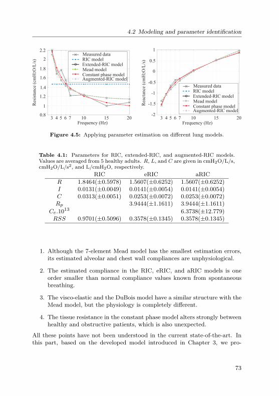
4.2 Modeling and parameter identification
0.5
1
0
-2
-0.5
-1
-1.5
3 4 5 6 7
Measured data
2015
2
2.2
1.8
1
1.6
1.4
1.2
0.8103 4 5 6 7
Frequency (Hz)201510
Res
ista
nce
(cm
HO
/L/s
)2
Rea
ctan
ce (
cmH
O/L
/s)
2
Extended-RIC modelRIC model
Mead modelConstant phase modelAugmented-RIC model
Frequency (Hz)
Measured data
Extended-RIC modelRIC model
Mead modelConstant phase modelAugmented-RIC model
Figure 4.5: Applying parameter estimation on different lung models.
Table 4.1: Parameters for RIC, extended-RIC, and augmented-RIC models.Values are averaged from 5 healthy adults. R, L, and C are given in cmH2O/L/s,cmH2O/L/s2, and L/cmH2O, respectively.
RIC eRIC aRICR 1.8464(±0.5978) 1.5607(±0.6252) 1.5607(±0.6252)I 0.0131(±0.0049) 0.0141(±0.0054) 0.0141(±0.0054)C 0.0313(±0.0051) 0.0253(±0.0072) 0.0253(±0.0072)Rp 3.9444(±1.1611) 3.9444(±1.1611)
Ce.1013 6.3738(±12.779)RSS 0.9701(±0.5096) 0.3578(±0.1345) 0.3578(±0.1345)
1. Although the 7-element Mead model has the smallest estimation errors,its estimated alveolar and chest wall compliances are unphysiological.
2. The estimated compliance in the RIC, eRIC, and aRIC models is oneorder smaller than normal compliance values known from spontaneousbreathing.
3. The visco-elastic and the DuBois model have a similar structure with theMead model, but the physiology is completely different.
4. The tissue resistance in the constant phase model alters strongly betweenhealthy and obstructive patients, which is also unexpected.
All these points have not been understood in the current state-of-the-art. Inthis part, based on the developed model introduced in Chapter 3, we pro-
73

4 Model-based parameter estimation with the forced oscillation technique (FOT)
pose physiological hypotheses and mathematical proofs to explain the abovementioned questions.
First simplification: from 9-element model to 7-element Mead models
The 9-element model, as developed in Chapter 3, is illustrated in Fig. 4.6. First
RcVFOT
ao
Rp
Cb
RcwCalv Cti Ccw
Cmouth
Iao Palv
P
Figure 4.6: The linearized lung model with 9 elements.
neglecting the cheek compliance Cmouth, the overall impedance is given as:
Z(jω) =Rc +jωI+Rcw +Rp− j
(ωR2
pCb + 1ωCalv
(CbCalv
+ 1))
(ωRpCb)2 +(CbCalv
+ 1)2 + 1
jωCti+ 1jωCcw
.
(4.9)Combining the central and chest wall resistances Rc+cw = Rc +Rcw, as well
as the tissue and chest wall compliances Cti+cw = CtiCcwCti+Ccw
, eq. (4.9) becomes:
Z(jω) =Rc+cw + jωI+Rp− j
(ωR2
pCb + 1ωCalv
(CbCalv
+ 1))
(ωRpCb)2 +(CbCalv
+ 1)2 + 1
jωCti+cw.
(4.10)Now, adding the cheek compliance Cmouth, the model structure (4.10) is iden-tical with the model of Mead (Fig. 4.3(K)). In other words, our model is indeedan extension of the Mead model. First, the central resistance as proposed byMead should contain thorax (and tissue) resistive components Rcw. Second,his proposed chest wall compliance Ccw should comprise the tissue elastanceCti as well.
74

4.2 Modeling and parameter identification
Second simplification: from 7-element Mead model to extended- andaugmented-RIC model
The bronchial compliance Cb is much smaller than the alveolar compliance Calv(eq. (3.3)): Vb
Valv(≈ 1/50− 1/30). Again, considering the impedance without
Cmouth, Z(jω) can be further simplified as:
Z(jω) =Rc+cw + jωI+Rp− j
(ωR2
pCb + 1ωCalv
))(ωRpCb)2 + 1 + 1
jωCti+cw, (4.11)
with the real partZR(ω) =Rc+cw + Rp
(ωRpCb)2 + 1 (4.12)
and the imaginary part
ZX(ω) = ωI−ωR2
pCb + 1ωCalv
(ωRpCb)2 + 1 −1
ωCti+cw. (4.13)
The imaginary part can be further simplified:
ZX(ω) = ωI−ω2R2
pCbCti+cw + Cti+cwCalv
− (ωRpCb)2−1
ωCti+cw((ωRpCb)2 + 1)
≈ ωI−ω2R2
pCbCti+cw− (ωRpCb)2
ωCti+cw((ωRpCb)2 + 1) , since Cti+cwCalv
≈ 1
≈ ωI−ω2R2
pCb(Cti+cw−Cb)ωCti+cw((ωRpCb)2 + 1) (4.14)
≈ ωI−ω2R2
pCbCti+cwωCti+cw((ωRpCb)2 + 1) , since Cti+cw Cb
≈ ωI−ωR2
pCb(ωRpCb)2 + 1 (4.15)
The derived real and imaginary parts (eq. (4.12) and (4.15)) are identical withthe extended-RIC model in eq. (4.7). Considering the parallel cheek complianceCmouth, we get the augmented-RIC model.This analysis yields two important scientific findings:
• The difference in the dimension (almost 30 -50 times larger) between the"large" compliances (alveolar, tissue, chest wall) and the small bronchial
75
4 Model-based parameter estimation with the forced oscillation technique (FOT)
compliance Cb leads to the dominance of Cb in the respiratory impedanceZ(jω). In other words, Z(jω) is not sensitive for the measurement of alve-olar, tissue, chest wall compliances. As a result, Calv and Ccw estimatedwith the Least-Squares method for the Mead model are unphysiologi-cal, as reported in the works of Diong [39] and Ionescu [84]. A detailedsensitivity analysis of the Mead model is given in Appendix A.4.
• The RIC, eRIC and aRIC models are simplifications of the Mead model.The "respiratory compliance" C in these three models corresponds to thebronchial compliance C = Cb. In other words, the compliance measuredby FOT and estimated with these three models is the bronchial compli-ance Cb. This explains why the compliance estimated in FOT (as shownin Section 4.2 or reported in [39, 84]) yield values which are one ordersmaller than typical value for lung compliance known from spontaneousbreathing and mechanical ventilation.
Physiological explanation of the DuBois, visco-elastic, and constant-phasemodels
The DuBois model has the Mead model’s parallel structure. However, thephysiological interpretation of the parameters is different: it comprises a tissuecompartment (Rti, Iti and Cti) instead of the peripheral and alveolar com-partment, a parallel gas compression compliance Cgas instead of Cb. In fact,after DuBois introduced this structure in 1956 [43], measurements publishedby other authors have shown that the influence of gas compression and tissueresistance is rather insignificant in FOT measurements. The gas compressioncompliance is estimated to be around 1/600L/kPa = 0.00017L/cmH20 [14] inhealthy adults, which is at least 20 times smaller than the normal value ofCb. If this compliance is indeed Cb, the other parallel branch must be the pe-ripheral and alveolar compartments, since a parallel structure between tissueand bronchi is unphysiological. Moreover, tissue resistance has also reportedto be small in several researches (1% [51], 7.41% [129], and 12.77% [31] of thetotal resistance, several times smaller than the estimated peripheral resistance.Hence, it cannot have a major contribution on the total resistance.The visco-elastic model also has Mead’s parallel structure. Its static com-
pliance Cs has exactly the same impact on the impedance as the chest wallcompliance Ccw in the Mead model, which is not sensitive in FOT measure-ments (eq. (4.15)). Its viscoelastic components Cve and Rve correspond toCalv and Rp in the Mead model. In other words, parameters estimated withthe visco-elastic model are identical with those of the Mead model (excludingthe inertance I). In my opinion, the visco-elastic model is rather a mathemat-
76

4.2 Modeling and parameter identification
ical approach than an useful model in respiratory modeling. It does not yieldany mathematical or physiological advantages against the Mead model.The constant-phase model does not have Mead’s parallel structure. This
model is indeed divided into one frequency-independent (airway) and one fre-quency-dependent part (tissue). In this model, the lung tissue is the onlycomponent which contributes to the frequency-dependency in ZR(ω). It alsoignores the impact of the parallel bronchial compliance to the frequency de-pendency [128] (which is, in my opinion, the main cause), and the chest wallcompartment. As a result, an overestimated tissue resistance is reported inpublications using this model (40% of the total resistance [93]). Moreover,scientists who support this model structure have been facing difficulties toconvince physiologists of the meaning of G and H, since they do not even havethe units of resistance and compliance [8]. When the lungs are challenged withbronchial agonists, G and H invariably increase even though only the airwayresistance and no tissue damping should be affected [15]. In fact, the changein G and H during bronchial challenges indicates the contribution of periph-eral airway resistance in G and H, which also questions the correctness of thismodel structure.
4.2.3 Model hierarchy and recommendationsIn the ATS/ERS official recommendations 2007 [19], the author stated: "Thefact that Rrs decreases with increasing frequency and approaches a plateauindicates the presence of parallel pathways. In children, the motion is per-haps the most significant factor [120]. In patients with airway obstructionor induced bronchi-constriction, peripheral inhomogeneity [118, 157, 200] andbronchial compliance [128] represent additional pathways. Elevation of Rrs to-ward lower frequencies, in other words, the contribution of tissue resistance,which has marked negative frequency dependence [189]. In healthy subjects,Rrs exhibits increase with frequency above 10 to 15 Hz: this is attributed tomultiple mechanisms, such as airway wall compliance, gas compressibility inthe central airways, and inertial distortion of the velocity profile [53].".There are two confusing points in this statement. First, it should be noted
that in Marchal et al.’s work [120], the authors performed FOT without cheeksupporting in purpose to demonstrate the influence of the upper shunt. In stan-dard FOT measurements, a reduction in Rrs was widely observed [100], evenwhen cheek vibration was reduced significantly by cheek supporting. Thus,the check motion is not the most significant factor in children. Second, thedocument recommends Mead’s idea of parallel peripheral airway, but also sup-port the constant-phase model which replaces Mead’s structure by a frequency-dependent tissue compartment in series. These two approaches have completely
77

4 Model-based parameter estimation with the forced oscillation technique (FOT)
different structure and physiological interpretation.Our comprehensive forward non-linear modeling supports the structure of
Mead. Figure 4.7 illustrates the relations among the models regarding linearity,model structure, and identifiability. As results of the model-based analysis, wepropose several recommendations for parameter identification in FOT:
Nonlinear two-degree-of-freedom model(Fig 3.11, this research)
Linear 9-element model(Fig 4.5, this research)
Mead‘s 7-element model
Extended-RIC model
Augmented-RIC model
RIC model
Visco-elastic model
Constant-phase model
Dubois‘s model
First simplificationR , Cticw
Second simplificationC ,Cti+cwalv
C for Hzf 20≤mouth
Simplification of
Addition of
Linearization,addition of L and C mouth
TissueGas compression
Nonlinear tissueNo gas compression
123456
: nonlinear: linear: Mead‘s parallel structure: serial structure: partly identifiable: completely identifiable
1,3,5
R p
Addition of R s
Same structure,differenrent
physiologicalinterpretation
2,3,5
2,3,5
2,3,6
2,3,6
2,4,6
2,3,5
1,4,6
2,3,5
Figure 4.7: Relation among models used in FOT measurements.
1. Mead’s parallel structure presents the best correspondence to lung phys-iology. The central resistance of the Mead model may comprise upperairway, lung tissue, and chest wall resistance in series. The chest wallcompliance may consist of tissue and chest wall compliances in series.
2. The alveolar, chest wall, and tissue compliances cannot be estimated withFOT. There is a leak in sensitivity in the measurement results regarding
78

4.3 The volume-dependent FOT
these parameters.
3. For FOT at frequencies above 3 Hz, the extended-RIC and the augmentedRIC models are recommended. These two simplifications of the Meadmodel are simple, identifiable, and deliver robust estimation results.
4. The compliance estimated by the eRIC and aRIC models corresponds tothe (peripheral) bronchial compliance, not the total respiratory compli-ance.
4.3 The volume-dependent FOT
Classic FOT focuses on the frequency-dependency of the respiratory impedanceZ(jω). However, since Z(jω) also depends on lung volume regarding the law ofHagen-Poiseuille, the change of Z(jω) over lung volume may provide additionalinformation on lung mechanics. Peslin et al. performed the Forced OscillationTechnique on 54 healthy subjects [164] in 1992. By applying the Rohrer’sequation directly on ZR(jω) in absence of a model structure and estimat-ing the flow- and volume-dependency of Z(jω), they reported an intra-breath(inspiration-expiration) variation of Z(jω). Nevertheless, these dependencieshave not gained any further attention, since the intra-breath changes are rela-tively small compared to the frequency-dependency for spontaneous breathing.
4.3.1 Principles of the volume-dependent FOTIn this section, we investigate the volume-dependency of Z(jω) over the wholelung volume. By introducing a new measurement protocol, an adapted dataanalysis, and a novel model-based parameter estimation, we propose a newextension of the classic FOT, which is given the name: volume-dependentFOT (v-FOT). The aims of the extension are to gain a deeper understandingof the physiological nature of Z(jω), and to find a more powerful tool to assessrespiratory mechanics.A v-FOT measurement is similar to a classic FOT with the following exten-
sions:
• During the measurements, subjects wear a nose-clip and support theircheeks to minimize the disturbances of the upper airways. After a fewcycles of spontaneous breathing, test subjects perform the so-called "slow-flow vital capacity maneuver". From the residual volume level, subjectsinhale slowly to total lung capacity, while FOT oscillation is superim-posed on the slow inhalation. A healthy subject may breathe in a respi-ratory volume of about 4-6 L in a time interval of about 5-6 seconds.
79

4 Model-based parameter estimation with the forced oscillation technique (FOT)
• Subjects are asked to perform the deep inspiration three times for eachoscillation frequency. The measurement should be repeated at differentoscillation frequencies between 3 Hz and 20 Hz.
• Optionally, v-FOT can also be performed during a slow expiration.
The above mentioned Butterworth bandpass filter can be used to extract thefrequency component at fos. The windowed cosine fitting method provides thedynamic changes of Z(jω) over time. Plotting Z(jω) over V provides a newpresentation of FOT, namely the impedance-volume (ZV) diagram. Lung vol-ume V forms the ordinate, while ZR(ω) and ZR(ω) are the abscissa. Hence, theimpedance measured via v-FOT comprises one more dimension: the volume-dependency Z(jω,V ).Figure 4.8 displays the measured (solid lines) and estimated ZV diagram
obtained on a healthy subject (male, 25 years old, BMI = 22.09). Least-Squaresparameter estimations are performed for the extended-RIC and constant-phasemodels. Data comprise ZR(jω,V ) and ZX(jω,V ) at all oscillation frequencies.While the constant-phase model yields a smaller error than the eRIC model,its estimated parameters are unphysiological (Raw < 0). In general, no volume-dependency can be estimated by these two models, the residual errors remainlarge, and the models’ behavior differ from the measurement data.
4.3.2 The reduced non-linear model
The linearization of the non-linear model discussed in Chapter 3.2.3 assumes asmall change of lung volume, such as in the spontaneous breathing and mechan-ical ventilation with normal tidal volume. Investigating the lungs over theirwhole volume, non-linear characteristics of the components should be consid-ered. While the bronchial, alveolar, and chest wall compliances, Cb, Calv, andCcw only become non-linear at extreme lung levels (Fig 3.7 and 3.11), the pe-ripheral resistance is volume-dependent due to Hagen-Poisseuille’s law over thewhole lung volume. Eq. (3.7) can be rewritten as:
Rp = 8µLπr4 = Kp
V −Voff, (4.16)
where Kp is a parameter characterizing Rp, and Voff is a shift in the measuredlung volume.For simplification, we consider only the volume-dependency of Rp in this
work. The eRIC and Mead model are extended to the volume-dependent eRICand Mead models (v-eRIC and v-Mead). The real and imaginary parts of the
80

4.3 The volume-dependent FOT
0 1 2 3 4 5
Volume - TV (L)
2
3
4
5
6
Rc = -6.8448G = 14.4067I = 0.0071766H = 2.0414S = 484.0497
0 1 2 3 4 5
Volume - TV (L)
2
3
4
5
6
ZR
(cm
H2O
/(L
/s)
R = 2.8269Rp = 2.7923I = -0.0016783C = 0.018158S = 503.7264
ZR
(cm
H2O
/L
/s)
eRIC
c
0 1 2 3 4 5
-4
-3
-2
-1
0
R = 2.8269Rp = 2.7923I = -0.0016783C = 0.018158S = 503.7264
0 1 2 3 4 5
-4
-3
-2
-1
0Z
X(c
mH
2O
/L/s
)
Rc = -6.8448G = 14.4067I = 0.0071766H = 2.0414S = 484.0497
Volume (L)- TV
Volume (L)- TV
c
b
b
constant-phase
3 Hz 5 Hz 7 Hz 10 Hz 15 Hz
ZX
(cm
H2O
/L/s
)measured
measured
measured
measured
eRIC
constant-phase
Real part Imaginary part
Figure 4.8: Measured (solid lines) and fitted (dashed lines) resistances andreactances measured with vFOT method. Data obtained from a healthy subject(male, 25 years old, BMI = 22.09), computed via Butterworth filtering andwindowed cosine fitting method. Least-Squares parameter fitting are performedfor the real and imaginary parts for the extended-RIC (eRIC) (top) and theconstant-phase models (bottom).
v-Mead model are given as:
ZR(ω,V ) = Rc+cw + Rp(ωRpCb)2 + 1
= Rc+cw + Kp(V −VOff)(ωCbKp)2 + (V −VOff)2 (4.17)
ZX(ω,V ) = ωI−ωK2
pCb + (V −VOff)2
ωCalv(ωCbKp)2 + (V −VOff)2 −
1ωCti+cw
. (4.18)
81

4 Model-based parameter estimation with the forced oscillation technique (FOT)
Frequency response of the system for critical frequencies: The frequencyresponses of ZR(ω,V ) for ω→ 0 and ω→∞ are given as follow:
ZR(ω = 0,V ) = Rc+cw + Kp(V −VOff) =Rc+cw +Rp =Rint (4.19)
ZR(ω→∞,V ) = limω→∞
(Rc+cw + Kp(V −VOff)
(ωCbKp)2 + (V −VOff)2
)= Rc+cw (4.20)
For ω → 0, ZR(ω = 0,V ) is equal to the sum of all resistive componentsof the respiratory system and equal to the resistance measured via the in-terrupter technique (Chapter 3.3). For ω →∞, the volume-dependency ofZR(ω = 0,V ) disappears and ZR comprises only the central and chest wallcompartments. The measurement results illustrated in 4.8 confirm our modelassumption. While ZR(ω = 3Hz,V ) is strongly volume-dependent, this depen-dency decreases massively at higher frequencies.These results can be used to augment the general explanation of R5 as the
total respiratory resistance and R20 as the central resistance, as commonlyknown in impulse oscillometry measurements [20,193]. It should also be clari-fied that both R5 and R20 comprise the chest wall resistance besides the centraland peripheral airway resistances, and thus are larger than the total airway re-sistance Raw measured with the body plethysmography (see Chapter 3.1).The Mead model assumes a parallel structure between Rp and Cb. Regarding
the more sophisticated Weibel model, the respiratory system can be seen asa distributed network of 23 RC-generations (Fig 4.9). Increasing the appliedfrequency, more and more peripheral bronchi lose their impact on ZR(ω =0,V ). Approximating the 23 RC-generation model by only one RC parallelstructure, a subdivision of the peripheral airways into large and small bronchi(Rlp and Rsp) will increase the accuracy of the model’s frequency response.The new model is called the v-Mead+ model. Applying the first and secondsimplification (eq. (4.15) and (4.10)) on the v-Mead+ model results in thev-eRIC+ model (Fig.4.9). The ZR(ω = 0,V ) of the v-eRIC+ is given as:
ZR,model(ω = 0,V ) = Rc+cw +Klp
V (t)−VOff+ Ksp(V (t)−VOff)
(ωCbKp)2 + (V (t)−VOff)2
= Rc+cw +Klp
V (t)−VOff+ KspV (t)−VOff
(4.21)
= Rc+cw +Rlp +Rsp (4.22)
with Rlp =Klp
V (t)−VOffand Rsp = Ksp
V (t)−VOff.
82

4.3 The volume-dependent FOT
RcV
Pmouth
Pmus
Rtr Rb1
Cb0
C20
RC- Generation model
Rb2
Cb1
Rb3
Cb2
R
R
ti
cw
Cb3
Calv(N=21-23)
R20
CtiC cw
L
RcV
Pmouth
Rlp Rsp
Cb
v-eRIC+ modelL
RcV
Pmouth
Pmus
Rlp Rsp
Cb
v-Mead+ model
R
R
ti
cw
Calv
CtiC cw
L
Fir
st a
nd s
econd
sim
pli
fica
tions
Fro
m d
istr
ibute
dto
conce
ntr
ated
Figure 4.9: Top: the RC-Generation model developed based on the Meadand Weibel models. Bottom: the extended volume-dependent Mead model (v-Mead+) with a large and a small peripheral resistance Rlp and Rsp.
4.3.3 Results of the parameter estimation
Again, we apply the non-linear Least-Squares fitting to estimate the param-eter of the v-RIC, v-Mead, and v-RIC+ models. For the v-RIC and Meadmodel, multi-frequency fitting is performed for ZR(ω,V ) and ZX(ω,V ). Pa-rameter vectors are θv−RIC = (Kp,Rc+cw,Cb,VOff , I)T ∈R1×5 and θv−Mead =(Kp,Rc+cw,Cb,VOff , I,Calv,Ccw)T ∈ R1×7.For the v-RIC+ model, we performed mono-frequency parameter fitting with
θv−RIC+ = (Klp,KspRc+cw,Cb,VOff)T ∈ R1×5 only for ZR(ω,V ) to increasethe fitting accuracy, since Klp and Ksp can alter by increasing frequencies.Figure 4.10 displays the results of the parameter estimation with the v-
eRIC, v-Mead, and v-eRIC+ models. Data are obtained from a healthy subject(male, 28 years old, BI = 23.15). The models are able to follow the volume-dependency of ZR(ω,V ) and ZX(ω,V ). All parameters estimated by the v-eRIC are in physiological ranges. There is no significant different in the residualerror between the v-eRIC and v-Mead model. As mentioned above, the "large"
83

4 Model-based parameter estimation with the forced oscillation technique (FOT)
0 2 4 60
5
10
15 K = 6.4494R = 1.7773C = 0.001495V = -0.25851I = 0.0025302S = 828.27
0 2 4 6
-4
-3
-2
-1
0
0 2 4 6
-4
-3
-2
-1
0
0 2 4 60
5
10
15
K = 6.4531R = 1.7765C
c+cw
= 0.0014949V = -0.25878I = 0.0025355C = -500C = -500S = 828.309
0 1 2 3 4 52
3
4
5
6
7
8
9
10Klp= 1.7696Ksp= 4.68Rc+cw= 1.7994C
off
= 0.0053685V = -0.1875S = 1.0458
v-M
ead
3 Hz 5 Hz 7 Hz 10 Hz 15 Hz
ZR
(cm
H2O
/(L
/s)
ZR
(cm
H2O
/(L
/s)
ZX
(cm
H2O
/L/s
)Z
X(c
mH
2O
/L/s
)
b
off
c+cw
cw
b
alv
p
p
off
Volume (L)
Volume (L)
Volume (L)
Volume (L)
b
Volume (L)
ZR
(cm
H2O
/(L
/s)
v-e
RIC
+v-e
RIC
Monofr
equen
cy f
itti
ng
Figure 4.10: Measured (solid lines) and fitted (dashed lines) resistances andreactances. Data obtained from a healthy subject (male, 28 years old, BMI= 23.15). Top and middle panels: Multi-frequency fitting for ZR(ω,V ) andZX(ω,V ), bottom panel: mono-frequency fitting for ZR(ω,V ) only.
84

4.4 The nasal FOT
compliances Calv and Ccw are estimated to unphysiological values which areat the boundary of the parameter vectors. This corresponds to the sensitivityanalysis of the Mead model as shown in Appendix A.4.The parameter estimation with the v-RIC+ model results in an extremely
small residual error S = 1.0458. The central resistance Rc is almost identicalwith that in the v-RIC and v-Mead models. All parameters are in physiologicalranges.Table 4.2 presents the average parameters obtained from one subject with
mild asthma and five healthy subjects. The large and small peripheral air-ways at functional residual capacity are computed according to eq. (4.16). Thecentral and chest wall tissue resistance Rc+cw is similar in both groups, whilehigher large and small bronchi resistances Rlp,FRC and Rsp,FRC, respectively,can be observed in the asthmatic volunteer. These results match the physio-logical expectation of an increase in peripheral bronchi in asthma.
Table 4.2: Respiratory parameters, measured with vFOT and estimated withthe e-RIC+ model.Parameter Rc+cw Cb Rlp,FRC Rsp,FRCUnit cmH2O/L/s L/cmH2O cmH2O/L/s cmH2O/L/s
Mild asthmatics 1.4 0.01064 0.77 2.78(n=1)Healthy subjects 1.45 0.00542 0.28 1.5(n=5)
4.4 The nasal FOT
Since FOT omits the necessity for cooperative maneuvers common in spirom-etry or body plethysmography procedures, it has a potential application forpatients with obstructive sleep apnea (OSA). However, since these patientsbreathe through their noses during sleep, the effect of the nasal passage andthe breathing mask on FOT measurements needs to be considered. Previ-ously, Farré et al. have carried out research using mono-frequency FOT and anesophageal balloon to investigate lung mechanics through a nasal mask [48–50].This section focuses on the compensation of the undetermined flow leakagecaused by using nasal masks and the influence of the nasal passage on multi-frequency FOT measurements. To determine the impedance of the nasal pas-sage, test subjects are asked to perform a FOT session with a Philips Respiron-ics ComfortGel Blue nasal mask (Philips Respironics, Pittsburgh, Pennsylva-
85

4 Model-based parameter estimation with the forced oscillation technique (FOT)
nia, USA). Impedance of nasal passage and nasal mask are computed by sub-tracting the total respiratory impedance (measured via nose) and the lowerrespiratory impedance (measured via mouth).
Compensation of gas leakage caused by using a nasal mask
The use of a nasal mask causes two different leakage sources: one at the CO2expiratory valve and one at the contact surface. The masks are fixed on thesubject’s face through elastic bands around the head. During the measure-ments, there is another leak around the top of the nose as well as in the cheekregion of the subjects (Fig. 4.11). Consequently, the flow entering the respi-ratory system Vrs and the flow measured by the pneumotach Vmeas are notthe same. The flow and leak components are illustrated in Fig. 4.12. Vvalve
Pdevice PmeasVmeas Vrs
Vvalve
Vleak
FOT-Device Nosemask Subject
. .
.
.
Figure 4.12: Schematic representing the leakage problem caused by using anasal mask.
is the flow through the expiratory valve and Vleak the flow leaking out at themask-face interface. Vmeas can be expressed as
Vmeas(t) = Vrs(t) + Vvalve(t) + Vleak(t) . (4.23)
Vleak is a mixture of laminar and turbulent flow. Its pressure-flow relationshipis given as the solution of the Rohrer equation (A.8):
Vleak(t) =− K12K2
+√
( K12K2
)2 + Ptrans(t)K2
, (4.24)
where K1 and K2 are laminar and turbulent coefficients. To estimate Vleak,the functional residual capacity of the lungs is assumed to be constant duringeach measurement. If all leakage has been compensated, the integrated lungvolume Vrs should be zero if the considered period [TStart,TEnd] is long:∫ TEnd
TStart
Vrs(t)dt= 0. (4.25)
86

4.4 The nasal FOT
The parametersK1 andK1 have been estimated using non-linear Least Squaresparameter estimation. The start valueK2,0 was estimated by running the LeastSquares algorithm only for K2 assuming K1 is equal to zero. After findingK2,0 = 500cmH2O/(L/s)2 and choosing K1,0 = 2cmH2O/L/s, the algorithmwas applied again on measurement data.
Figure 4.11: Air leaks out at respiratory valveand at mask-face interface [144].
The corrected volume of arepresentative measurementis depicted in Fig. 4.13. Af-ter the correction of thevalve Vvalve(t), there is stillapproximately 1.5L gas in-side the lungs, which corre-sponds to the amount of airleaked out at the mask-faceinterface. Tab. 4.3 showsthe parameters of the leak-age compensation. The pa-rameter K2 of the turbulentflow dominated that of thelaminar flow at face-mask-interface.
5
Volu
me
(L)
-1
0
1
2
3
4
5
6
7
8
After compensation of expiratory valve flowAfter total leakage correction
10 15 20 25 30
Before correction
Time (s)
Figure 4.13: One representative result of the leakage compensation: volumesbefore correction, after compensation of the expiratory valve and after totalleakage correction for TEnd = 31s [144].
Results of the nasal FOT measurements
Applying FOT at patients’ mouth and nose in two different measurementsdemonstrates the effect of the nasal passage and mask on FOT results (see
87

4 Model-based parameter estimation with the forced oscillation technique (FOT)
Frequency K1 K2 RSS[Hz] [cmH2O/l/s] [cmH2O/(l/s)2]5 0.0101 1298.8130 3.4524 · 10-17
6 0.0438 2125.8626 2.1192 · 10-21
7 0.0102 1306.4878 4.1273 · 10-17
8 0.0760 2255.9254 8.5190 · 10-21
10 0.0098 695.2472 5.8974 · 10-21
15 0.0080 863.1106 5.1379 · 10-20
Table 4.3: K1 and K2 for compensation of leakage at mask-face interface.
RVnose I
CRnawI naw
(for example: RIC model)
mouthnasal airways (naw)
total respiratory system
lower respiratory system (lrs)
Figure 4.14: Model of the nasal airways and the lower respiratory system.
Fig. 4.15). The average resistance and reactance of the lower (lrs) and totalrespiratory system for all test subjects are depicted in Fig. 4.15. Both resis-tances ZR,total and ZR,lrs decreased over frequency. ZX,lrs yields a positivefrequency dependence from −1.159cmH2O/l/s at 3Hz to 1.176cmH2O/l/s at20Hz. ZR,total is significantly higher than ZR,lrs. Resonance frequency arefound to be between 7.5Hz and 9.5Hz for the lower respiratory system, whichcorrelates to the results reported by MacLeod and Birch [119]. For the totalsystem, the average resonance frequency decreases to 4Hz.
Tab. 4.4 displays the values of the nasal (naw) resistance ZR,naw and theratio ZR,naw/ZR,total. ZR,naw is computed by subtracting ZR,total by ZR,lrs.The nasal resistance has an average value of 4.096± 2.019cmH2O/l/s whichcorresponds to 66% of the total resistance. Our measurement confirms theresults reported in [51] (Fig.3.12) and indicates that the nasal impedance has alarge contribution in the total respiratory impedance and cannot be neglectedin nasal FOT measurements.
88

4.5 Summary
-3
-2
-1
0
1
2
34
Frequency [Hz]3
ZR
[cm
H O
/L/s
2
4
6
8
10
12
Total respiratory system Lower respiratory system
2015104 5 6 70
2
ZX
[cm
H O
/L/s
2
Frequency [Hz]3 2015104 5 6 7
Figure 4.15: Average resistance and reactance of the total and lower respiratorysystem.
ID Rnaw Rnaw/Rtotal[%] Inaw Inaw/Itotal[%]1 3.3412 58.58 0.0091 30.332 2.7237 65.32 0.0134 52.343 2.8278 61.01 0.0178 58.174 4.5795 70.44 0.0136 49.645 8.5902 73.41 0.0418 78.426 2.3394 61.46 0.0118 56.737 6.3148 83.58 0.01487 65.228 2.0484 57.08 0.01043 53.49
Mean 4.096 66.36 0.0166 55.54±STD 2.019 7.91 0.00985 12.8
Table 4.4: Rnaw and proportion of Rnaw to Rrs. Resistances are given incmH2O/L/s and inertances are given in cmH2O/L/s2.
4.5 Summary
This chapter presents a comprehensive investigation on the respiratory impe-dance measured via the forced oscillation technique. The windowed cosinefitting method is applied on the bandpass-filtered data to compute the respira-tory impedance. The physiological interpretation of the impedance relates tothe underlying model structure. The Mead model present the best correspon-dence to respiratory mechanics. The extended- and augmented-RIC modelsdeliver robust estimation results. The estimated compliance with these twomodels corresponds to the elasticity of the peripheral bronchi, not the alveolior tissue.The volume-dependent FOT is an extension of the classic FOT. It measures
the change of the impedance over frequencies and lung volume. The ZV di-
89

4 Model-based parameter estimation with the forced oscillation technique (FOT)
agram provides additional lung information to assess lung mechanics. It hasbeen show that the extended respiratory models v-eRIC, v-Mead, and v-eRIC+can be used to describe the volume-dependency of the impedance.
90

5 Modeling of cardiopulmonary interactions andcardiogenic congestion
Breathing in, I am aware of my heart.Breathing out, I smile to my heart.
Thich Nhat Hanh
Cardiopulmonary interactions are indispensable in living beings. Despitemany studies on animal and clinical data over the past 50 years, these inter-actions are only partly understood, especially under pathological conditions ormedical treatments. Moreover, there is a lack of computational models whichcan simulate these interactions quantitatively. This chapter introduces a bio-physical forward model of the cardiopulmonary system which focuses on thehemodynamic interactions between the lungs and the heart. First, a cardio-vascular model developed in Matlab Simscape™ is introduced. Second, modelvalidations comparing simulation results with clinical and animal data are dis-cussed. Finally, the model is extended by the lymphatics and the fluid balancesystem to explain the development of heart failure and cardiogenic congestion.Parts of the chapter were previously published in peer-reviewed journals [142,
150].
5.1 Modeling of heart and circulation
The development of the cardiovascular model is based on the works of Smithet al. [191,192] with several extensions. In the first model extension, the atriawill be considered explicitly. Second, non-linear behaviors of the veins andthe pulmonary capillaries will be taken into consideration. The comprehensivestructure of the cardiovascular model and the overall model is illustrated inFig 5.1.
5.1.1 Atria, ventricles and heart valves
The heart model consists of left atrium (la), right atrium (ra), left ventriclefree wall (lvf), right ventricle free wall (rv), septum (spt), pericardium (pcd)and four heart valves (pulmonary valve Rpv, bicuspid valve Rmt, tricuspidvalve Rtc and aortic valve Rav). The atria and ventricles are modeled byelastic elements (compliance). Their PV relationships are characterized by theend-diastolic pressure-volume relationship (EDPVR) and end-systolic pressure-volume relationship (ESPVR) [77,153,192]. Let Ees be the chamber elastanceduring systole and Vd its filling volume of the ESPVR at zero transmural
91

5 Modeling of cardiopulmonary interactions and cardiogenic congestion
P
e(t)
e(t)
e(t)
+
-
+
-
+
-
+
-
+
-
+
-
+-
+
-
e(t)
mo
uth
/atmo
sph
ere
muscles
c(t)
c(t)
+
-
+
-
+
-
+
-
+
-
+
-
ao
Pv
c
tricusp
id v
alve
aortic
valv
e
pu
l. capillaries
mitral v
alve
Pra
Plv
system
icv
eno
us
com
pl.
system
icarterialco
mp
l.
aortic
resistance
e(t)
+-
e(t)e(t)
+
-
e(t)
+
-
left ven
triclefree w
all
pericard
ium
leftatriu
m
septu
m
righ
t ven
triclefree w
all
righ
tatriu
m
Hea
rtP
ulm
on
ary
circula
tion
+
-
pu
l. valv
e
Prv
Pla
+
-
+
-
pu
l. ven
ou
scap
illaries
pu
l. ven
ou
s
pu
l. arteries
Pp
a
Pp
v
Pp
vc
pu
l. arterialcap
illaries
Sy
stemic
circula
tion
Pleu
ral sp
ace
Pp
l
Pin
t
Pm
us
PP
E
Pleu
ral
spa
ce
Interstitium
+
-
+
-
rigid
airway
s
collap
s.airw
ays
lun
g tissu
eco
mp
.
Pa
lv
collap
s.airw
ays
com
p.
alveo
larco
mp
.
chest w
allco
mp
.
blo
od
flow
air flow
heartb
eatresp
iratory
mu
scles
Din
Do
ut
Resp
irato
rysy
stem
+
-
+
-
aortic
com
plian
ce
+
-
system
icin
ertance
system
icresistan
ce
+
-
aortic
inertan
ce
Figure
5.1:The
overallmodel,consisting
oftheheart,the
systemicand
pulmonary
circulation,andthe
respiratorysystem
.Flow
sare
distinguishedbetw
eenblood
flow(red
arrows),air
flow(blue
arrows).
92

5.1 Modeling of heart and circulation
pressure, P0 the minimal diastolic pressure, λ the curvature of the EDPVRcurve, and V0 atrium volume at zero pressure, then the PV relationships aregiven as [192]:
Pes = Ees · (V −Vd), (5.1)
Ped = P0 · (eλ(V−V0)−1). (5.2)
A time-variant driver function e(t) activates either eq. (5.1) or eq. (5.2) tomodel the transition between the systolic and diastolic pressures:
P (V,t) = e(t) ·Pes(V,t) +(1−e(t)) ·Ped(V,t). (5.3)
Table 5.1: Transmitting resistances ofheart valves [cmH2O/L/s]
Resistance
Tricuspid 4.0789
Pulmonary 2.7191
Mitral 13.5955
Aortic 6.7977
The driver function e(t) can bemodeled as a Gauss distribution foratria, and as a sum of four dif-ferent Gauss distributions for ven-tricles and septum. Parametersof e(t) are taken from [153] andgiven in Appendix A.5. Theheart valves are modeled with idealdiodes with transmitting pressures of10−5 cmH2O, blocking resistances of105 cmH2O/L/s, and various trans-mitting resistances (Table 5.1) [191].
5.1.2 Septum and pericardiumSeptum and pericardium cause ven-tricular interactions which have astrong impact on cardiovascular dynamics. Smith et al. [192] separated theventricles into three free wall components: left ventricle free wall (lvf), septum(spt), and right ventricle free wall (rvf). No component has an influence on theother parts. The septum moves leftward towards the left ventricle during sys-tole and rightward towards the right ventricle during diastole. The ventricularvolume is a combination of the septum and ventricular free wall volume. Theseptum is driven by the same driver function as the left ventricle.The pericardium is a double-wall sac surrounding four heart chambers and
separating them from the pleural space. The pericardium volume is, hence,the sum of ventricular and atrial volumes. In our model, the pericardium ismodeled by one compliance; its positive terminal is connected to the pleuralspace and its negative terminal to the four heart chambers.
93

5 Modeling of cardiopulmonary interactions and cardiogenic congestion
5.1.3 Vascular arteries and veinsThe vascular system, a network of blood vessels, is modeled by lumped elementsregarding its function rather than its anatomical structure [33, 89, 117, 192].Realistic values of cardiac preload and afterload can be determined by applyingthe Windkessel model to the systemic and pulmonary circulation [192]. Whilethe aorta and arteries are linearized with parameters adapted from [36], it isnecessary to consider the non-linearities of the veins [68,69,75,96,191,223,227,230]. According to Hainsworth [69] and Rothe [179], the pressure-volume (PV)characteristics of a vessel can be divided into different phases: collapsed, filling,unstressed, distention, and over-distension (Fig. 5.2).
0
Volu
me
Transmural pressure
2
Volu
me
(L)
00
4
1
3
0-10 10 20 4030
0-10 10 20 4030
Transmural pressure (cmH O)2
0.5
0.25
0.75
0
1
2
1
3
Collapsed
Filling
Over-distension
Distension
Unstressed
Systemic veins
Pulmonary veins
Figure 5.2: (1) Pressure-volume (PV) characteristics of a collapsible tube,reproduced from [69]. (2) PV relation of the systemic veins. (3) PV relation ofthe pulmonary vein [142].
The nonlinear behavior of the veins can be modeled by the log function
V = 1λ· log(Ptr + P0) +V0, (5.4)
including the three parameters P0, V0 and λ. The log function has a highgradient at the beginning which changes quickly to a lower slope after the "un-stressed" point. The parameters are obtained for 3 L systemic venous blood
94

5.1 Modeling of heart and circulation
volume and 300 mL pulmonary venous blood volume at normal blood pres-sures [96]. Figure 5.2 compares the PV characteristics of a separated vesselreported in [69] and the implemented systemic and pulmonary veins.Unlike the separated vessel, the veins must maintain a nonzero volume even
at zero or negative transmural pressure, since they are networks of vesselstethered to the surrounding tissues which prevent them from a total col-lapse [37, 69, 179]. The minimum volume of the systemic veins is positive andconsidered to be 1 L in the model. Under normal conditions, there is around3 L in the systemic veins under a slightly positive transmural venous pressure.
Pulmonary capillaries
The pulmonary capillaries surround the lung alveoli. Their PV characteristicscan be modeled by the hyperbolic function:
Vcap(t) = V0 + 1λ· tanh(c ·Ptr,cap(t) +P0). (5.5)
The constant parameter V0, c, and P0 are determined based on followingconsiderations [68,96]:
1. In a healthy body, the pulmonary capillary transmural pressure is Ptr,cap≈15 cmH2O (= Pcap−Pint = 10− (−5) cmH2O), where Pcap is the pres-sure inside the lung capillaries and Pint the pressure of the surroundinginterstitial pressure.
2. At this pressure level, a total blood volume in the pulmonary circulationis approx. 200 mL.
3. At normal transmural pressure, the capillaries can be modeled by an idealcompliance with a linear PV relationship. At immoderately low pressure,the capillaries collapse to a minimum volume of approx. Vmin = 10 mL.At excessively high pressure, all capillaries are recruited and assumed toreach a maximum volume of 400 mL.
For a detailed description of CPIs and congestion, the pulmonary capillarycompliance is subdivided into arterial and venous capillary components. Bothtogether simulate the total PV characteristics shown in Fig. 5.3.Unlike the peripheral airways, the length of the pulmonary capillaries can
be considered to be unchanged during respiratory activities. Thus, accordingto the law of Poiseuille, flow resistance of the lungs capillaries R(t) is inverselyproportional to the square of their volume:
R(t) = R1 ·(V1−0.9Vmin)2
(V (t)−0.9Vmin)2 . (5.6)
95

5 Modeling of cardiopulmonary interactions and cardiogenic congestion
-20 -10 0 10 20 30 40 50
Pressure (cmH2O)
0
0.2
0.4
Vo
lum
e (L
)
pulmonary capillaries
Figure 5.3: PV-characteristics of lung capillaries [142].
Vmin is the minimal capillary volume during collapse. V1 and R1 are capillaryresistance and volume at a normal transmural pressure, respectively. Param-eters for the pulmonary capillaries are given in Table 5.2. At a normal fillingvolume V = 200 mL, the pulmonary flow resistance is 69.75 cmH2OL−1 s, whichreaches a maximum value of R= 2.5∗106 cmH2OL−1 s at a collapsing volumeof V = Vmin = 10 mL.
Table 5.2: Parameters of the pulmonary capillaries. V1, V0, and Vmin aregiven in L, R1 in cmH2OL−1 s, and λ in L−1. c is a scalar.
Resistance ComplianceParameter Value Unit Parameter Value Unit
V1 0.2 L V0 0.1025 LR1 70.8725 cmH2OL−1 s P0 -1.3687 cmH2O
Vmin 0.005 L λ 10.256 L−1
c 0.0821 1
The remaining linear parameters of the systemic and pulmonary circulationare given in Table 5.3. At the beginning of the simulation, each complianceis assgined to an initial volume. Each heart ventricle has an initial volumeof 40 mL. The systemic veins are filled with 3.1 L, the systemic arteries andcapillaries with 600 mL. On the pulmonary side, initial volume is set to 100mL for the arteries, 100 mL for the capillaries, and 50 mL for the veins.
5.1.4 Baseline simulation of the cardiovascular systemBaseline simulations were performed to validate the model for a healthy subject.The change in the systemic arterial volume during the initial phase is depictedin Fig. 5.4. At the beginning of each simulation, blood redistributes regarding
96

5.1 Modeling of heart and circulation
Table 5.3: Parameters of systemic and pulmonary circulation, from [36,191].Components Param. Value Unit
aortic compliance Cao 0.000168 LcmH2O−1
syst. arteries compliance Csys,art 0.0011 LcmH2O−1
aortic resistance Rao 91.78 cmH2OL−1 ssyst. resistance Rsys 1359.5 cmH2OL−1 saortic inertance Lao 1.1216 cmH2OL−1 s2
syst. inertance Lsys 4894.4 cmH2OL−1 s2
pul. art. resistance Rpa 94.5 cmH2OL−1 spul. art. compliance Cpa 0.0022 LcmH2O−1
pul. ven. resistance Rpv 31.5 cmH2OL−1 s
the ratio between the vessels’ compliances. At t= 20 s and t= 25 s, the driverfunctions of the ventricles and atria are activated, respectively. The operatingpoint of the system, where all compliances have reached their steady-statevolume have, is arrived after approx. 40 seconds.
0 10
time (s)
0.6
0.8
1
1.2
vo
lum
e(L
)
5020 30 40 60 70 80
Figure 5.4: Changes in systemic arterial volume during the initial phase of thesimulation. From a start value at 0.6 L, the volume reached a stationary valueof 1.2 L. After the heart started to pump at t = 20 s, the volume stabilized ataround 1.05-1.09 L.
Figure 5.5 presents the simulated pressures and volumes during three cardiaccycles in a healthy person. Heart rate is 80 beats per min, stroke volume 72mL, and cardiac output 5.76 L/min. The aortic pressure rises to 169 cmH2O(124.3 mmHg) in systole and falls to 110 cmH2O (80.9 mmHg) in diastole.Table 5.4 compares the simulated blood pressures and cardiac indexes to
the standard range of a healthy person [78]. Cardiac and stroke indexes arecalculated by assuming a total body surface of 1.73 m2. All simulated valuescorrespond to physiological standard ranges provided in literature. The blood
97
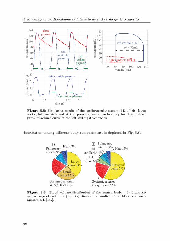
5 Modeling of cardiopulmonary interactions and cardiogenic congestion
0
20
40
60
80
100
120
140
pre
ssure
(m
mH
g)
aorticpressure
leftventriclepressure
leftatrium
pressure
0 0.5 1 1.5 2time (s)
0
10
20
30
pre
ssure
(m
mH
g)
right ventricle pressure
right atrium pressure
sv = 72mL
40 60 80 100 120 140volume (mL)
0
20
40
60
80
100
120
140
pre
ssure
(m
mH
g)
left ventricle (lv)
right ventricle (rv)
Figure 5.5: Simulative results of the cardiovascular system [142]. Left charts:aortic, left ventricle and atrium pressure over three heart cycles. Right chart:pressure-volume curve of the left and right ventricles.
distribution among different body compartments is depicted in Fig. 5.6.
Heart 5%
Pulmonaryarteries 5%
Pul.capillaries 4%
Pul.veins 6%
Systemic arteries& capillaries 22%
Systemicveins 58%
Heart 7%Pulmonaryvessels 9%
Systemic arteries,& capillaies 20%
Smallveins 25%
Largeveins 39%
21
Figure 5.6: Blood volume distribution of the human body. (1) Literaturevalues, reproduced from [68]. (2) Simulation results. Total blood volume isapprox. 5 L [142].
98

5.2 Cardiopulmonary hemodynamic interactions
Parameter Model Standard [78] UnitPressures:Left ventricle systolic 124 90 – 140 mmHgLeft ventricle end-diastolic 6 5 – 12 mmHgLeft atrial 3.5 – 5 2 – 12 mmHgArterial systolic 122 90 – 140 mmHgArterial diastolic 81 60 – 90 mmHgRight ventricle systolic 25 18 – 30 mmHgRight ventricle end-diastolic 0.5 -0.5 – 4.5 mmHgRight atrial mean 0 -2 – 2 mmHgPulm. artery systolic 26 13 – 30 mmHgPulm. artery diastolic 11 3 – 15 mmHgPulm. capillary wedge max 10 – 16 8 – 23 mmHgPulm. capillary wedge min 6 – 11 5 – 14 mmHgOthers:Cardiac index 3.33 2.5 – 5.3 L/min/m2
Stroke index 41.63 37– 72 mL/beat/m2
Table 5.4: Baseline simulation results of pressures, cardiac and stroke indexes.The indexes were calculated with a total body surface of 1.73 m2. Standardvalues are given in [78].
5.2 Cardiopulmonary hemodynamic interactions
This section focuses on the mechanical coupling between the respiratory andthe circulatory system. The pericardium, pulmonary arteries and veins aresurrounded by the pleural pressure Ppl, while the pulmonary capillaries aresurrounded by the interstitial pressure Pint. The coupling is implemented inSimscape by means of physical connections between the two subsystems. Theoverall system is presented in Fig. 5.1.Under normal conditions, the thoracic blood volume (TBV) is about 20%
(approx. 1 L) of the total blood volume [68,96]. The chest wall capacity (Vcw)from eq. (3.15) has to be adapted, since Athanasiades et al. [4] did not considerTBV in their model and assumed that the maximal chest wall volume was equalto the total lung capacity (TLC). In our model, Vcw,max has been adapted toTLC +1 L, the parameter Bcw in eq. (3.16) is changed to
Bcw ≈Vmax−RV4 ·Ccw,max
≈ 4.75 cmH2O. (5.7)
The new parameters of the chest wall are given in Table 5.5. The initial value
99
5 Modeling of cardiopulmonary interactions and cardiogenic congestion
of chest wall volume increases to 2.05 L by taking the TBV into consideration.
Table 5.5: Adaptation of the chest wall parameter with regard to thoracicblood volume from the respiratory to cardiopulmonary system.
Parameter RS only CPS UnitAcw 7 7 cmH2OBcw 3.5 4.75 cmH2OVmax 5.6 6.6 LRV 1.3 1.3 LPPE 10 10 cmH2O
In summary, the comprehensive cardiopulmonary model consists of a 8-element non-linear respiratory model and a cardiovascular model with fourheart chambers, hearts valves, a systemic and a pulmonary circulation [142,148]. The respiratory and the cardiovascular system are coupled at the pleuralspace and lung interstitium.
5.2.1 Simulation resultsThe simulation results are compared to clinical data and animal studies re-ported in literature. Since model parameters can vary among species andindividuals, parameter estimation can increase the performance of the modelin curve fitting. However, changing randomized parameters via "try and error"in such a large model can lead to parameter "manipulation". For that reason,all parameters are remained unchanged during all simulations. Only the inputsignal, the respiratory muscles are adapted to generate the required scenariosby changing the pleural pressure during spontaneous breathing and the mouthpressure during mechanical ventilation.
Mueller maneuver
During spontaneous inspiration, a decrease in Ppl leads to a shift in bloodvolume from the systemic to the pulmonary circulation and a fall in aorticpressure. During inspiration with maximum effort (Mueller maneuver1), a sig-nificant increase in aortic pressure, transmural left and right ventricular filling
1During Mueller maneuver, subjects are asked to perform a forced expiratory. After that,an attempt at further inspiration is made with closed mouth and nose, which makesthe thoracic pressure maximal subatmospheric. Mueller maneuver can be used in theevaluation of airway obstruction in patients with sleep apnea [194].
100

5.2 Cardiopulmonary hemodynamic interactions
pressure during the Mueller maneuver in closed-chest, anesthetized, neurallyintact Mongrel dogs was documented by Robotham et al. [175]. Inactivatingthe respiratory tract due to zero gas flow, and setting the pleural pressure from0 to −12 cmH2O and back to 0 within a duration of 8 heart beats, the initialcondition of the Mueller maneuver occurs.
6080
100
50
100
150
-20
0
20
Pre
ssure
(m
mH
g)
-5
0
510
120 124 128 132 136 140
120140160
-20
0
20
0
10
20
Pre
ssure
(m
mH
g)
P - Pla
P - Pra
2s Time (s)
138
87
-12
13.54.8
142
94
2.912.3
-12
8.9 15.52.65
3.88
Transmural aortic
Transmuralleft artrial
Pleural
Transmuralright atrial
21
Ppl
P - Pao pl
pl
pl
Figure 5.7: Pressure relations during a Mueller maneuver. The pleural pres-sure, as well as transmural aortic, left and right atrial pressures are depicted.(1) Data measured on a neurally intact Mongrel dog, reproduced from [176].(2): Model simulation results for a healthy human. The pleural pressure in themodel was set from 0 to -12 cmH2O and back to 0 within 8 heart beats [142].
Figure 5.7 depicts simulation results (2) in comparison with animal data (1).At the second heart beat after the end of the maneuver, the transmural aorticpressure reaches its maximum at 138 mmHg (142 mmHg in animal data) . Thetransmural right atrial pressure rises during the first 5 heart beats, and fallsabruptly to a negative value. The transmural left atrial pressure also increasesand reaches it maximum about 3 heart beats later than the transmural rightatrial pressure. Dynamic behaviors of the model is observed to be similar toanimal data.
Pressure relations during ventilation
A ventilator is connected to the cardiopulmonary system to simulate the model’sresponse to mechanical ventilation. Fig 5.8 (1) depicts data from a lung-diseased patient under volume-controlled-ventilation (VCV) published by Jardinet al. [90]. Electrocardiogram (ECG), airway (A), esophageal (E), right atrial(RA), and pulmonary capillary wedge (PCW) pressures were simultaneouslyrecorded. Tidal volume was set to 12 mL/kg (equivalent to 840 mL for a 75 kg
101

5 Modeling of cardiopulmonary interactions and cardiogenic congestion
Pre
ssu
re (
cmH
O)
2
1
-5
0
10
20
30
40
45
RA
PCW
A
E
-10
0
10
20
30
40
50
ra
cap
3
1s
Airways
Pleural
Paw
Ppl
Right atrial P
CapillaryP
Driver function e(t)
-10
0
10
20
30
40
50
-10
0
10
20
30
40
50
Pre
ssu
re (
cmH
O)
2 Paw
capPcapP
raPraP
PplPpl
2ECG peak
V = 840 mL,10% lung compliance
T
V = 3.2 LT
V = 840 mLT 4a
Paw
V 840 mLT ≈
0
0.05
0.1
0.15Left ventricular
Right ventricular
Vo
lum
e (L
)
4b
Figure 5.8: Pulmonary and cardiovascular pressures in patients under volume-controlled ventilation (VCV). (1): Data reproduced from [90]. PCW = pul-monary capillary wedge pressure, RA = right atrial pressure, A = airway pres-sure, E = esophageal pressure. (2,3,4): simulative results: (2) VT = 3.2 L (3)VT = 840 mL volume. (4a) VT = 840 mL and reduction of lung compliance by90%. (4b) Left and right ventricular volume for simulation (4) [142].
102

5.2 Cardiopulmonary hemodynamic interactions
patient). Peak ventilation pressure was 45 cmH2O. Figures 5.8 (2-4) displaythe simulation data for different tidal volumes. In (2), VT is set to 3.2 L toachieve a peak pressure at 45 cmH2O. Simulation (3) is done for VT = 840 mL,which results in a peak airway pressure < 10 cmH2O. These results show thatsuch a high ventilation pressure at a low tidal volume does not occur in healthysubjects. The high pressure-volume ratio indicates a dramatic drop in the lungcompliance, such as in a severe restrictive pulmonary disease. Reducing thelung compliance (alveolar and tissue compliance) to 10% of the original values,a peak pressure of 45 cmH2O can be achieved at VT = 840 mL as shown in 5.8(4a).
44 46 48 500
25
50
75
100
125
150
175
200
44 46 48 50
Time (s)
-10
0
10
20
30
40
P
P
P
E Ppl
2
-10
0
10
20
30
40
Pre
ssu
re (
cmH
2O
)P
ress
ure
(cm
H2
O)
0
25
50
75
100
125
150
175
200
ao
pa
Pul. arterial systole
Systemic arterial systole
Systemic arterial diastole
cap
ao
1
A
PCW
Ppl
Paw
Pul. arterial diastole
ΔPsa,1ΔPsa,2
ΔPsa,2ΔPsa,1
ΔPpa,1 ΔPpa,2
ΔPpa,1ΔPpa,2
9 heart beats
Figure 5.9: Aortic, pulmonary arterial and capil-lary pressure during a ventilation cycle. (1) Clini-cal data, reproduced from [90]. (2) Simulative re-sults. Observation: ∆Psa,1 <∆Psa,2 and ∆Ppa,1 >∆Ppa,2 [142].
Simulation corresponds tothe prediction of a restric-tive condition in this pa-tient. Furthermore, Jardinobserved that the increasein the pulmonary capillarywedge pressure (PCW) isgreater than that in theesophageal pressure, whichleads to an increased left ven-tricular volume; and the in-crease in right atrial pres-sure is smaller than that inesophageal pressure, whichcorresponds to a decreasein right ventricular volume.The pressure relations (∆Pcap> ∆Ppl > ∆Pra) can bereproduced by the model.Figure 5.8 (4b) displays thechange in left and rightventricular volumes duringVCV. An increase in left ven-tricular volume and a de-crease in right ventricularvolume can be quantitativelyobserved in the model response.In the same paper, Jardin et al. performed a beat-to-beat analysis on data
from 13 ventilated patients, focusing on the change in systemic and pulmonaryarterial pressure during ventilated inhalation (Fig. 5.9 (1)). During the lunginflation, esophageal pressure Ppl increased slightly less than PCW. An in-
103

5 Modeling of cardiopulmonary interactions and cardiogenic congestion
crease in systemic arterial pressure was reported, where systole was greaterthan diastole. There was also an increase in the pulmonary arterial pressure,however, change in diastole was greater than in systole. Testing the model withthe same scenario, simulation results yield similar behaviors. Figure 5.9 de-picts the systole-diastole gradient in systemic and pulmonary arterial pressure,where ∆Psa,1 <∆Psa,2 and ∆Ppa,1 >∆Ppa,2. The model response correspondsto the reported clinical data.
Stroke volume during spontaneous breathing and positive-pressureventilation
This part compares the change of stroke volume (SV) between spontaneousbreathing and positive-pressure ventilation. In anesthetized, intact canines,differential effects of negative (spontaneous inspiration) and positive (positive-pressure inspiration) changes in the intra-thoracic pressure on cardiovascu-lar dynamics were reported [64, 167, 168]. While the left ventricular SV fallswith positive pressure inspiration, the right ventricular SV behaved inversely.Fig. 5.10 compares animal data (1) and simulation results (2). The left andright ventricular SV is large in human (50 - 60 mL) comparing to those of acanine (15 - 18 mL). During a positive-pressure inspiration, right ventricularSV first decreases, then increases back to the previous value. This behaviorcan be observed in animal data and simulation results.
-10
0
10
20
10
15
20
25SVvr
1015
20
25
-10
0
10
(cm
H2O
)
40
60(mL
) stroke volume left ventricle
50
100stroke volume right ventricle
In. In.Ex.
pleural pressure
(mL
)
Ex. In. Ex. In. Ex.
PCV
airway pressure
Spontaneous breathingPCVSpontaneous breathing
5s
SVlr
Paw
Ppl
PplPaw
SVrv
SVlv
21
Figure 5.10: Cardiopulmonary interactions during spontaneous breathing andmechanical ventilation. (1) cardiopulmonary interactions observed in animalexperiment reported in [64,168]. (2): model simulation results [142].
Cherpanath et al. introduced a schematic diagram to study CPIs duringmechanical ventilation [30] (Fig. 5.11). He qualitatively proposed two causesfor the fall of left ventricular SV during positive-pressure ventilation. On theone hand, a higher lung volume causes an increase in the intra-thoracic pressure
104

5.2 Cardiopulmonary hemodynamic interactions
(IIP), which reduces venous return and right ventricular preload. On the otherhand, a rise in airway pressure leads to an increase in transpulmonary pressure(TPP), followed by an increase in pulmonary vascular resistance and a risein right ventricular afterload. The diagram is extended quantitatively withmodel’s responses, as shown in Fig. 5.11. The preload is presented by end-diastolic ventricular volume, the afterload by the arterial pressure.
Lungvolume↑
Mechanicalventilation
TPP↑ PVR↑RV
Afterload↑
Airwaypressure↑
ITP↑Venousreturn↓
RVPreload↓
RV strokevolume ↓
LV strokevolume ↓
0 10→
2.45 3.65 L→
-5.6 -1.3→ cmH O2
150 500→
cmH O/l/s2
5 9→
cmH O2
0.69 -0.24 L/s→ 0.053 → 0.041 L
31-36 → 27-36
cmH O2
63-72 → 54-60 mL
55-74 → 32-69 mL
cmH O2
↑
Figure 5.11: Change right and left ventricular stroke volumes under mechanicalventilation. Schema adapted from [30]. Numerical values are from a simulationwith pressure-controlled ventilation at PIP=10 cmH2O [142].
Simulation results confirm the Cherpanath’s diagram, with an exception of avariable right ventricular afterload, which does not increase under mechanicalventilation. These results gives an evidence to support the hypothesis, thatthe changes observed in left and right ventricular SV are primarily caused bythe reduction in venous return and right ventricular preload, and less by thechange in right ventricular afterload, as proposed in other literatures [64,166].
Effect of PEEP on CPIs
A correlation between PEEP and pleural, transpulmonary, pulmonary arterial,and right atrial pressures was documented by Scharf et al. in anesthetizedMongrel dogs (22−25 kg) [182]. The animals were under VCV (VT = 300−350mL (12−14 mL/kg)), PEEP was set to be 0.6, 4.3, 7.7, 11.4, and 16.4 cmH2O.A comparison between animal data and model response is depicted in Fig. 5.12.Tidal volume VT was set to 12.7 mL/kg (equivalent to 950 mL for a 75 kghealthy human).Simulation results correlate well with animal data. With increasing PEEP,
a rise in lung volume, and further increases in transpulmonary, pleural, pul-
105

5 Modeling of cardiopulmonary interactions and cardiogenic congestion
0 5 10 15
0
5
10
15
Pre
ssure
(m
mH
g)
0
0.5
1
0 5 10 15PEEP
101214161820222426
2030405060708090100
0 5 10 15
0
4
810
0
0.5
1
1.5
2
0 5 10 15PEEP
16
20
60708090100
2
-2
12
4
86
PTP
PPL
∆V
PPA
PRA
CO
% c
ontr
ol
PPA
PRA
CO
∆lu
ng v
olu
me
(L)
PTP
PPL
∆V
CO
2
Pre
ssure
(m
mH
g)
21
Figure 5.12: Effect of PEEP on lung volume, cardiac output (CO), transpul-monary (TP), pleural (PL), pulmonary arterial (PA), and right atrial (RA) pres-sures during volume-controlled ventilation. (1) Experimental data in Mongreldogs, data reproduced from [182], (2) Simulation results [142].
monary arterial, and right atrial pressures can be observed in both data. AsPEEP increases from 0.6 to 16.4 cmH2O, cardiac output falls to 35% of theoriginal value in dogs and to 65% in simulated human. Note that a better fitbetween data and model may be achieved by adjusting the parameters of themodel. However, this is not the objective of this forward modeling.
5.3 The fluid balance and the lymphatic system
5.3.1 Model development
Modeling of the Starling-equation and the fluid transport
In 1896, Ernest Starling stated that the fluid movement across a vascularbarrier would cease when the hydrostatic forces and interstitial osmotic pres-sures are in balance [197]. This hypothesis, verified by Landis several decades
106

5.3 The fluid balance and the lymphatic system
later [104,105], is known as the Starling equation:
J =Kf [(Pcap−Pint)−σ · (Posm,cap−Posm,int)]. (5.8)
Here, J (in [mol/s]) is the total flux of molecules from the capillaries to thelung interstitium, Kf is the permeability of the capillary walls, and σ is theosmotic reflection coefficient for large proteins. Pcap and Pint are the capillaryand interstitial hydrostatic pressures, and Posm,cap and Posm,int are the corre-sponding colloid osmotic pressures, respectively. Typical parameter values ofeq. (5.8) are given in Table 5.6.
Table 5.6: Typical parameters of the Starling equationParameter Value Unit ReferenceKf 10−6 LcmH2O−1 s−1 [68] [217] [136]Pcap 10 cmH2O [222] [68]Pint -5 cmH2O [109] [228]σ 0.75 1 [109] [136]Posm,cap 38.07 cmH2O [68]Posm,int 19.04 cmH2O [68]
In literature, the protein reflection coefficient σ was reported to be betweenσ = 0.7 [109] and σ = 0.8 [136]. The osmotic pressure depends on the proteinconcentration in blood. Its typical values are 28 mmHg at artery end and 14mmHg at venous end of the pulmonary capillaries [68]. The determinationof the permeability Kf is difficult. In animals experiments, a typical valueof Kf = 10−6 LcmH2O−1 s−1 was estimated by measuring the hydrostaticpressures and the lymphatic flux [68,135,217]. This flux can be easily removedby the lymphatic system under normal conditions. The permeability Kf isthe product of the hydraulic conductivity K and the filtration surface area A.Assuming a cylindric form for the capillaries with a length l and a radius r, arelation between Kf and the capillary volume Vcap can be derived as
Kf =K ·A=K ·2πl =K ·2√π · l ·Vcap. (5.9)
Then the hydraulic membrane resistance RStarling is given as:
RStarling = 1Kf
= 1K ·2
√π · l ·Vcap
. (5.10)
107

5 Modeling of cardiopulmonary interactions and cardiogenic congestion
The Starling equation (5.8) yields:
J = 1RStarling
[(Pcap−Pint)−4Pos], (5.11)
where4Pos = σ ·(Posm,cap−Posm,int) is the osmotic pressure gradient betweenthe pulmonary capillaries and the lung interstitium.
pulmonary capillaries R_starling
+
-
Δ P_oslung interstitium
Figure 5.13: Electrical equivalent representationof the Starling equation.
arteriole venule
lymph-capillaries
re-absorptionca. 10%
ca. 90%
Pulmonary interstitium
filtration
arterialcapillary
re-absorption
venouscapillary
Figure 5.14: Filtration and resorption at capillaryendothelial wall, modified from [184].
Eq. (5.11) states a corre-lation of the flux througha membrane and the mem-brane’s transmural pressuregradient, similar to Ohm’slaw for an electrical cur-rent. In this work, the fil-tration is modeled by a cur-rent flow through an electri-cal resistance, as illustratedin Fig. 5.13. Note that 4Poswas implemented as a DC-pressure source and set in se-ries with RStarling.The fluid transport, illus-
trated in Fig. 5.14, is acontinuous process. Fluidflux changes from positiveat the arterial capillary end(filtration) to negative atthe venous capillary end (re-absorption) due to the pressure relations [184]. In normal conditions, 90% ofthe flux is reabsorbed at the venous capillaries. The other 10% is removed bythe lymphatic system. In our model, the capillary compartment is subdividedinto an arterial and a venous part (Rcap,art and Rcap,ven) (see eq. 5.15). Theresistances can be derived as
RStarling,art = R1,art ·√
V1,artVcap,art
, RStarling,ven = R1,ven ·√
V1,venVcap,ven
, (5.12)
where Vcap,art and Vcap,ven are the volume of the arterial and venous capillaries.R1,art, V1,art, R1,ven and V1,ven are constant parameters. These parameters,given in Tab. 5.7, were calculated considering following factors:
108

5.3 The fluid balance and the lymphatic system
• The sum of the arterial and venous Starting resistance is equal the totalStarling resistance of the capillaries.
RStarling = RStarling,art +RStarling,ven
= R1,art ·√
V1,artVcap,art
) +(R1,ven ·√
V1,venVcap,ven
)
• Hydraulic conductivity at capillary venous end is 40% higher than oneat capillary arterial end [109].
Once the fluid has entered the lung interstitium, it continues moving forwardto the peribronchovascular space, where it is absorbed by the lymphatics. Thequantitative behavior of extracellular fluid movement in the interstitium is notwell understood, as well as any influence of this resistance to the development ofpulmonary edema or the absorption over the lymphatics [202]. In this work, thehydraulic resistance for fluid movement within interstitium (see Fig. 5.15) wasassumed to be Rint = 1000 cmH2OL−1 s. The large value of Rint is considered,since the flow resistance within interstitium can be neglected in comparison tothe trans-membrane Starling resistances. Table 5.7 summarizes the parametersof the model.
Table 5.7: Parameters of the implemented Starling equationParameter Value UnitR1,art 2.4∗106 cmH2OL−1 sV1,art 0.12 LR1,ven 1.7∗106 cmH2OL−1 sV1,ven 0.08 L4Posm 14.27 cmH2ORint 1000 cmH2OL−1 s
A model of the lymphatic system
The lymphatic pump and flow resistance are modeled by a parallel structureof a compliance and a resistance. The fluid flow entering the lymph Iin,lym isgiven as
Iin,lym = 1Rint
· (Pint−Plym), (5.13)
109

5 Modeling of cardiopulmonary interactions and cardiogenic congestion
valve out
RP
ulm
onary
capillaries
+
-
+
-
+
-
+-
blood flow
liquid flow
Arteries
Starling, ven
I cap, art
Pint
I cap, ven
I cap
R
Vlym
Vcap, ven
Δ Posm, ven
Δ Posm, artRStarling, art
flow
resistance
Veins
Capillarybarrier
Interstitium
int
R int
R lym
+
-
valve in
Vcap, art
Lymph
d(t)lymphatic
pump
d(t) lymph pump
P vena cava
Figure 5.15: The lymphatic system from pulmonary interstitium to vena cava.The Starling equation is implemented at arterial and venous ends of the pul-monary capillaries.
where Plym is the lymphatic pressure. The volume-pressure characteristics ofthe lymphatic pump is modeled, similarly to the heart pump, with an driverfunction d(t). d(t) switches the contraction of the lymphatic collector from anactive to a passive phase and vice versa:
Vlym = (1−d(t))(ln(Plym + P0,lym)
λlym+ V0,lym) +d(t) · (
PlymEes,lym
+ Vd,lym),
where Vlym is the lymphatic volume. The parameters λlym, P0,lym and V0,lymdefine the passive, Ees,lym and Vd,lym the active phase of the pump (Tab. 5.8).
The driver function d(t) realizes a switch between a diastolic and systolicphase of the lymphatic pump (see Fig. 5.16). While the heart rate is given by
110

5.3 The fluid balance and the lymphatic system
78 80 82 84 86 88
Time (s)
0
0.5
1
d(t
)
driver function lymphs
Figure 5.16: Driver function d(t) of the lymphatic pump. A pumping cycle is2 second long. The maximum frequency of the pump is 12 beat per minute.
the sinus node and thus, volume-independent, the activation of the lymphaticpump depends on its filling volume Vliq [184]. There is less known about theregulation of the lymphatic pump [202]. The maximal transport capacity ofthe lymph within the lungs differs strongly among different references and alsovaries for specific lung pathologies. It is reported to be higher in chronic heartfailure or mechanical damages of the pulmonary capillaries than in hydrostaticedema [68, 202]. In this work, the maximal flow was derived due to the safetyfactor introduced in [68, 202]. In fact, the lymphatic system is able to removethe extra fluid filtration, which is caused by an increase in the pulmonaryvenous hydrostatic pressure by 5 mmHg. This elevation causes an extra fluxof approx. 6.8∗10−6 Ls−1, according to the Starling-equation. The maximumpump frequency is 12 beat per minute [184], which leads to an amount of3.4∗10−5 L removed per lymphatic contraction. The pressure-volume behaviorof the pump is illustrated in Fig. 5.17.
0 1 2 3 4 5 6
Volume (10 -5 l)
0
5
10
15
Pre
ssure
(cm
H2O
)
lymphatic pump
-5SV = 3,518 10 l
Figure 5.17: PV-curve of the lymph during a contraction
The lymphatic stroke volume is 3.518∗10−5 L. At a pump rate of 12 beatsper minute, the maximum possible absorption rate is 25.3 mLh−1 or 607.9 mL
111

5 Modeling of cardiopulmonary interactions and cardiogenic congestion
per day.
Parameter Value UnitRlym 1 cmH2OL−1 sVd,lym 0 LEes,lym 106 cmH2OL−1
V0,lym 8.731∗10−5 LP0,lym 0.1527 cmH2Oλlym 50364 L−1
Rint 103 cmH2OL−1 sPvalve,in 10−6 cmH2OPvalve,in 10 cmH2O
Table 5.8: Parameters of the lymphatic model
Similar to the structure of the systemic veins, lymphatic flows are unidirec-tional due to the non-return valves located along the lymphatic vessels. Inour model, these valves were modeled by two diodes (valve in and valve out,see Fig. 5.15). The overall model is illustrated in Fig. 5.18. The sophisticatedmodel includes three different hydraulic media: blood flow in the circulation,air flow in the respiration, and fluid flow in the lymphatics. The interstitialpressure Pint is connected to all three systems.
5.3.2 Model extension for cardiogenic pulmonary congestion
During pulmonary congestion, the accumulated fluid affects the mechanics ofthe lungs. Healthy human lungs with a dry weight of 1000 g [5] and a wet-dry-relation of W
D ≈ 4 ggdry
[109] contain approx. 800mL fluid in the intra-and extracellular spaces. A acute pulmonary edema occurs by an increase ofinterstitial fluid increases by 25 to 35% (+ 200 bis 300 mL) [21,109,202].
The lung tissue during congestion
As the interstitial pressure Pint rises, the fluid amount within the lung tissuealso increases. The maximal fluid volume is reached when (1) lung tissue is notable to capture more fluid and (2) bronchial and alveolar edema occur [109].In our model, the lung tissue compliance is extended to depend on the fluid
112

5.3 The fluid balance and the lymphatic system
P
+
-
ao
Pvc
tric
usp
id v
alv
e
aort
icv
alv
em
itra
l v
alv
e
Pra Plv
syst
emic
ven
ou
sco
mp
l.
syst
emic
resi
stan
ce
left
ven
tric
lefr
ee w
all
rig
ht
per
icar
diu
m
left
atri
um
sep
tumrig
ht
ven
tric
lefr
ee w
all
left
per
icar
diu
m
rig
ht
atri
umH
eart
Pu
lmon
ary
circ
ula
tion
pu
l. v
alv
e
Prv
Pla
pu
l. v
eno
us
com
pl.
pu
l. a
rter
ies
Pp
a
Pp
v
Pp
vc
Syst
emic
circ
ula
tion
Ple
ura
l sp
ace
Ple
ura
lsp
ace
Inte
rsti
tium
blo
od
flow
air
flow
Res
pir
atory
syst
em
+
-
+
-
Pm
us
PP
E
mouth
Rc
Rp
Cb
Cal
v
Pal
v
Vb
Pin
t Cti C
cw
Flu
idb
ala
nce
fluid
flow
resp
irat
ory
dri
ve
+
-
syst
emic
arte
rial
com
pl.
aort
icre
sist
ance
+
-
aort
icco
mp
lian
ce
+
-
aort
icin
erta
nce
c(t)
e(t)
e(t)
e(t)
e(t)
c(t)
+
-
R
Capillaries
+
-
+
-
+
-
+
-
+
-
+
-
+
-
+
-
Sta
rlin
g, ven
Ica
p, ar
t
Pin
t
I cap, venIca
pR
Vly
m
Vca
p, ven
ΔP o
sm, ven
ΔP o
sm, ar
tR
Sta
rlin
g, ar
t
flow resistance
Cap
illa
rybar
rier
Inte
rsti
tium
int
+
-
Rin
t
Rly
m
+
-
Vca
p, ar
t
Lym
ph
d(t
)
hea
rtbea
te(
t)ly
mphat
icpum
pd
(t)
Fig
ure
5.18
:The
overallm
odel,c
onsistingof
theheart,
thesystem
ican
dpu
lmon
arycirculation,
therespiratory
system
,and
theflu
idba
lance.
Flowsaredistingu
ishedbe
tweenbloo
dflo
w(red
arrows),a
irflo
w(bluearrows)
and
fluid
flow
(green
arrows).
113

5 Modeling of cardiopulmonary interactions and cardiogenic congestion
amount accumulated in the lung interstitium:
4Ptr,ti = 1Cti·Vlung + Psafe · (1−e−20·Vliq ), (5.14)
where Vliq presents the extra-fluid amount inside the lung interstitium. Psafeis the maximum pressure gradient caused by the change in tissue elasticity.Ptr,ti presents the transmural pressure of the lung interstitium and equals thedifference between the pleural and interstitial pressure (Ptr,ti = Ppl −Pint).Psafe is determined to be 9.5 cmH2O due to the maximum rise in interstitialpressure 4Pint = 6.8 cmH2O. Fig. 5.19 illustrates the influence of Vliq on thePV characteristics of the tissue component.
0 1 2 3 4 5 6 7 8 9 10 11 12 13 14 15
Ptr,ti
(cmH O)2
0
1
2
3
4
5
6
lung v
olu
me
(L)
PV diagram lung tissue
V = 0liq +10ml +20ml +50ml +100ml
+200ml
+250ml
Figure 5.19: The shift of the PV characteristics of the tissue component re-garding the interstitial liquid amount Vliq during the development of pulmonarycongestion.
The osmotic pressure during congestion
The critical venous pressure at which fluid starts to accumulate in interstitiumis defined as the safety factor in pulmonary edema [68]. A rise in the pulmonaryvenous pressure by 13.6 cmH2O (10 mmHg) is critical before an alveolar edemaoccurs [68, 202]. Note that the safety factor of 13.6 cmH2O is without a con-sideration of the osmotic pressure, which can be up to 50% of the total safetyfactor (20mmHg) [68, 109]. Indeed, as the fluid amount accumulated in thelung interstitium rises, the protein concentration and the interstitial osmoticpressure Posm,int decrease, which leads to a reduction of the fluid filtrationregarding the Starling equation. To compensate the safety factor difference, areduction of the osmotic gradient 4Posm,int = 13.6 cmH2O/σ ≈ 18.1 cmH2Ois considered. This corresponds to a reduction of almost 100% of the osmoticpressure (Posm,int = 19 cmH2O).
114

5.3 The fluid balance and the lymphatic system
In this work, a polynomial function of second order was used to model thedependency of the osmotic pressure on the filtration rate [202]:
Posm,int = Posm,int,0 · (1−√
VliqVliq,max
). (5.15)
Posm,int,0 = 19 cmH2O presents the constant osmotic pressure without extrafluid filtration, Vliq,max is the critical fluid amount (Vliq,max = 250 mL).
The alveolar and bronchial flooding
In later stages of pulmonary congestion, the distal bronchi and alveoli arefilled with fluid and collapse due to a reduction of surface tension [21,109]. Thepressure-volume characteristics of edematous bronchi and alveoli are character-ized by an increase in the threshold opening pressure (TOP) and a reduction ofthe compliance due to decreased surfactant concentration [21,32,32,228]. An-imal trials predict a change of TOP up to 20 cmH2O [111]. In the model, thechange in the pressure-volume relationship of the alveoli and bronchi duringpulmonary edema is considered to be dependent on the fluid amount accumu-lated in interstitial space Vliq. If Vliq exceeds 250 mL, an edema occurs in thealveoli and peripheral bronchi (see Fig. 5.20). The alveolar TOP increases by4PTOP = 10 cmH2O and the maximum alveoli compliance Calv,max decreasesby half of its value, from 0.3 to 0.15 LcmH2O−1. The parameter λ of theperipheral bronchi (eq. (3.11)) increases from 18.38 to 36.76 L−1.
-20 0 20 40
Pressure (cmH2O)
0
2
4
6
Volu
me
(L)
alveoli
-10 0 10 20 30
Pressure (cmH2O)
0
0.05
0.1
Volu
me
(L)
peripheral bronchi
V > 0,25 LV > 0,25 Lliq
liq
Figure 5.20: Alteration in the PV characteristics of the peripheral bronchi andthe alveoli during edema. If the interstitial fluid amount exceeds a critical valueVliq > 250 mL, their PV curves shift to the right, TOP increases and compliancesfall.
When a bronchial airway collapses, the fluid film surrounding the inner wallof the bronchi causes the bronchi to stick together. To reverse this process,
115
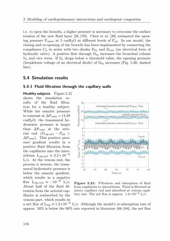
5 Modeling of cardiopulmonary interactions and cardiogenic congestion
i.e. to open the bronchi, a higher pressure is necessary to overcome the surfacetension of the new fluid layer [28, 170]. Chen et al. [28] estimated the open-ing pressure Popen at 5 cmH2O at different levels of Ppl. In our model, theclosing and re-opening of the bronchi has been implemented by connecting thecompliance Cb in series with two diodes Din and Dout (an electrical form ofhydraulic valve). A positive flow through Din increases the bronchial volumeVb and vice versa. If Vb drops below a threshold value, the opening pressure(breakdown voltage of an electrical diode) of Din increases (Fig. 5.20, dashedline).
5.4 Simulation results
5.4.1 Fluid filtration through the capillary walls
0
10
20
30
Pre
ssu
re (
cmH
O)
2
30 35 40 45 50 55 60
Time (s)
-5
-4
-3
-2
-1
0
1
2
3
4
5
Flo
w (
10
-6L
/s)
osmotic pressure (P )osm
transmural pressure venous end (P - P )cap,ven int
transmural pressure arterial end (P - P )cap,art int
Icap,art
Icap,ven
Icap
Figure 5.21: Filtration and absorption of fluidfrom capillaries to interstitium. Fluid is filtrated atartery capillary end and absorbed at venous capil-lary end. The net flux is approx. 1.2 ∗ 10−6 L/s.
Healthy subjects Figure 5.21shows the simulation re-sults of the fluid filtra-tion for a healthy subject.While the osmotic pressureis constant at ∆Posm = 14.28cmH2O, the transmural hy-drostatic pressure is largerthan ∆Posm at the arte-rial end (Pcap,art − Pint >∆Posm). This positive pres-sure gradient results in apositive fluid filtration fromthe capillaries into the inter-stitium Icap,art ≈ 2.2 ∗ 10−6
L/s. At the venous end, theprocess is inverse; the trans-mural hydrostatic pressure isbelow the osmotic gradient,which results in a negativeflux Icap,ven ≈ −10−6 L/s.About half of the fluid fil-tration from the arterial cap-illaries is reabsorbed by thevenous part, which results ina net flux of Icap ≈ 1.2∗10−6 L/s. Although the model’s re-absorption rate ofapprox. 50% is below the 90% rate reported in literature [68,184], the net flux
116

5.4 Simulation results
of 1.2∗10−6 L/s conforms the works of Miserocchi [135] and Wangensteen [217].These authors reported a daily fluid amount of 103.7 mL fluid filtration fromthe pulmonary capillaries to the interstitial space.
0
10
20
30
Pre
ssu
re (
cmH
O)
2
30 35 40 45 50 55 60
Time (s)
-5
0
5
10
15
20
Flo
w (
10
-6L
/s)
transmural pressure venous end
transmural pressure arterial end
osmotic pressure
Icap
Icap,art
Icap,ven
Figure 5.22: Change in capillary pressure andblood flow in heart failure. Blood flow becomespositive at the venous capillary end. There is anadditional fluid filtration to the interstitial insteadof re-absorption. Regarding the high permeabilityof the capillaries at the venous end, the venous fluxexceeds the flux at the arterial capillary end. Thetotal flux increases from 1.25∗10−6 L/s to 15∗10−6
L/s.
Heart failure Cardiogenic fail-ure leads to an elevated pres-sure in pulmonary circula-tion and a rise in fluid fil-tration. The simulation ofa left ventricular dysfunctioncan be performed by reduc-ing the elasticity of the leftventricle Ees,lvf . Figure 5.22presents the pressure andvolume changes during a sim-ulated sudden heart failure,where Ees,lvf falls to 20% ofit maximal value.
The transmural pressureat the arterial end rises fromapprox. 19.5 to 26.7 cmH2O,the filtrated flow increasesby 3.8 ∗ 10−6 to 6.0 ∗ 10−6
L/s. At the venous endof the capillaries, the trans-mural pressure increases to25.09 cmH2O, and thereforeto values larger than the av-erage osmotic gradient. Forhealthy subjects, the absorp-tion process at venous endbecomes an additional filtra-tion process due to the ele-vated hydrostatic pressure. The amount of fluid filtrated at the venous endeven exceeds the amount at the artery end, which correlates to the observationof Lenfant et al. [109]. The reason for this high filtration is the high permeabil-ity of the capillaries at the venous end [109]. The net flux is Icap ≈ 15∗10−6
L/s, which results in 1296 mL within 24 hours.
117

5 Modeling of cardiopulmonary interactions and cardiogenic congestion
5.4.2 Lymphatic absorption
To demonstrate the lymphatic response to the change in pulmonary bloodpressure, simulations has been performed for different grades of heart failure.The ventricle’s elasticity Ees,lvf has been reduced to 35% at t1 = 100 s and to20% at t1 = 200 s, as shown in Fig. 5.23.
0
10
20
(cm
HO
)2
0 50 100 150 200 250 300
Time (s)
0
0.5
1
1.5
2
Volu
me
(mL
)
lymph pulse
Vlym
Vliq
Vcap
pulmonary venous pressure
7,677,26
t1 t2
Figure 5.23: Filtration volume at different levelsof the pulmonary venous pressure.
As a result of heart fail-ure, the pulmonary venouspressure increases by 7.67cmH2O after t1 and again by7.26 cmH2O after t2. Thegradient of the volume curveVcap corresponds to a posi-tive fluid filtration from thecapillaries to lung intersti-tium. The first pressure ele-vation after t1 does not causea fluid accumulation in inter-stitial space due to an adap-tion of the lymphatic systemby increasing the pump fre-quency. While the pump isactivated only once betweent = 50 s and 100 s, its raterises to approx. 0.18 Hz af-ter t1.After t2, the lymphatic
pump rate rises to 0.2 Hz andachieves its maximum capac-ity. However, the pump is not able to remove all the fluid filtration. Thesimulation yield a safety factor of 7.67 cmH2O. This safety factor is slightlyabove literature values (6.8 cmH2O). After t2, a positive change in edema-tous fluid by 0.4 mLmin−1 is predicted by the model. The simulation resultsshows that fluid filtration can be removed back to the systemic circulation viathe lymphatic system, as long as the safety factor regarding the pulmonarypressure is maintained.
5.4.3 Cardiogenic pulmonary congestion and CPAP treatment
This part demonstrates the model behavior in the development of cardiogenicpulmonary congestion and the effect of CPAP treatment via a long time sim-
118

5.4 Simulation results
ulation (for over 90 hours). A heart failure with reduced Ees,lvf to 10% ofthe normal value [83] was modeled at t = 12 hours which directly causes anincrease in the pulmonary blood pressures, and later, a lung congestion. ACPAP treatment was started at t = 60 hours to demonstrate the effect of thetherapy in lung congestion. Simulation results are displayed in Fig. 5.24, 5.26,and 5.25.By reducing the elastance of the left ventricle to 10% of the normal value,
the venous pressure rose by 25 cmH2O and as result, the cardiac stroke volumefell from 5.8 to 2.2 L/min. The intrathoracic blood volume (ITBV) increasedby 400 mL to 1.05 L. The extra tissue liquid Vliq rose from 0 to 221 mL within12 hours, but is still below the critical volume of 250 mL (Fig. 5.24). Sincehormonal and neural regulation is not considered in the model, cardiac outputremained at a low level. The average interstitial pressure Pint increased from−6.5 cmH2O at the beginning of the simulation to −0.5 cmH2O 12 hours afterthe heart failure.In the respiratory system, the pleural pressure Ppl fell from −7.5 cmH2O
to −10.5 cmH2O. The transmural pressure over lung tissue Ptr,ti rose from1 to 10 cmH2O. Implementing the same respiratory muscles activity for thewhole simulation, tidal volume fell from 0.5 L by almost 60% to 0.23 L. Thestatic PV characteristics of the respiratory system moved rightward due to thechange in the lung compliance (Fig. 5.26). The total compliance of the systemwas 25% smaller at point 2 (pulmonary congestion) than in point 1 (healthy).The lung volume at FRC also fell by 1.1 L to 1.5 L.The reduction of the lung volume during pulmonary congestion depends on
two factors. First, the extra interstitial fluid reduces the tissue complianceCti and make the lungs "stiffer" (Fig. 5.19). Second, a rise in total thoracicblood volume suppresses the lungs and make it harder to expand. Since thechest wall and the lung compliances are approx. the same, a rise by 400 mL inITBV results in a decrease of 200 mL in lung volume and an increase of 200mL in chest wall volume (Fig. 5.25). In reality, an adaption of the respiratorymuscles is required to maintain a normal lung volume and gas exchange, whichincreases the work of breathing and makes breathing heavier for patients withcongestive diseases.At t = 60 h, a CPAP therapy with a PEEP of 10 cmH2O has been started.
PEEP had an immediate effect on the respiratory system: lung volume cameback to its normal value of 2.5 L at FRC. The tidal volume normalized at500mL. The PEEP compensates the transmural pressure Ptissue, which in-creased due to the fluid filtration into the interstitium. The pleural pressurealso returned back to its normal value and the system moved back to its nor-mal operating point (point 3). Vliq fell from 221mL to 3mL within 12 hours.ITBV fell by 150mL, the pulmonary blood pressure decreased by 7 cmH2O.
119

5 Modeling of cardiopulmonary interactions and cardiogenic congestion
12 24 36 48 60 720
1
2
3
4
5
6V
olu
me
(l)
12 24 36 48 60 72-15
-10
-5
0
5
10
Pre
ssure
(cm
H2O
)
0
10
20
30
40
50
Pre
ssure
(cm
H2O
)
0
0.125
0.25
Volu
me
(l)
0.5
0.75
1
1.25
1.5
Volu
me
(l)
12 24 36 48 60 72
Time (h)
1.8
2
2.2
2.4
I (l
/min
)
0.05
0.1
0.15
0.2
Volu
me
(l)
12 24 36 48 60 72
Time (h)
0.2
0.3
0.4
0.5
0.6
Volu
me
(l)
12 24 36 48 60 72
0
5
10
15
Pre
ssure
(cm
H2O
)
mech. ventilation (CPAP)ventricle volumeleft
right
pulmonary venous pressure
+ 25 cmH2O
total thoracic blood volume
+ 400 ml
extra tissue liquid (V )
221 ml
lung pressures
P
P
P
lung volume
chest wall volume
blood
1,05 l
cardiac output5,8 l/min activity)
1,5 l
- 7 cmH2O
- 150 ml
- 100 ml/min
- 12,5 ml
- 6 ml
(same muscletidal volume
tr,ti
pl
int
liq
Figure 5.24: Simulation result of lung congestion. At t=12 h, heart failureis stimulated by reducing left ventricle elasticity to 10% of the original value.Pulmonary blood volume and pressures increases, while cardiac output falls.After 60 hours (2 days after occurrence of heart failure), a treatment with CPAPtherapy (PEEP = 10 cmH2O) is initiated simulatively.
The simulation predicts that the use of CPAP leads to an immediate normal-ization of ventilation. The rise in the pleural and interstitial pressures viaCPAP "presses" the fluid out of interstitium and reduces ITBV.
120

5.4 Simulation results
11,5 12 12,5 13
Time (h)
2
2.5
3
3.5
4
4.5
Vol
ume
(l)
11,5 12 12,5 13
Time (h)
0.6
0.8
1
1.2
1.4
Vol
ume
(l)
pulmonary volumestotal thoracic blood volume
+ 400 ml
- 200 ml
+ 200 mlchest wall
lung
Figure 5.25: Change in ITBV, lung and thorax volume during pulmonarycongestion. The change at t = 12 h relates to the shift in ITBV. The slowerchange after t = 12 h relates to the change in lung tissue compliance regardingthe fluid accumulation in interstitium.
-20 0 20 40
Pressure (cmH2O)
1
2
3
4
5
Vol
ume
(l)
pulmonary congestion
-20 0 20 40
Pressure (cmH2O)
1
2
3
4
5
Vol
ume
(l)
healthy
1
4
2
3
cw
lung
cw + lung
V_liq = 221 ml
Figure 5.26: Static PV-characteristics of the respiratory system. Four opera-tion points are marked during the simulation. Point 1: healthy, during the first12 hours. Point 2: At t = 36 h, 24 hours under pulmonary congestion. Point3: short after started CPAP therapy with PEEP= 10 cmH2O. Point 4: after 12hours of CPAP therapy.
While the use of CPAP obviously improves the respiration, it has a negativeimpact on the cardiac output, as expected. While a left heart failure alreadyreduces the preload of the right ventricle, the use of CPAP increases the intrathoracic pressures and the afterload of the right ventricle, which causes a furtherreduction in the cardiac output. In the simulation, cardiac output fell from 2.2per minute to 2 liter per min during the use of CPAP 5.24.
121

5 Modeling of cardiopulmonary interactions and cardiogenic congestion
5.5 Discussion and summary
This chapter introduces a comprehensive model of the hemodynamic interac-tion between the lungs and the cardiovascular system. The overall model in-cludes more than 30 elements. Simulation speed was 30 times faster than realtime (on a PC with Intel Core i7-4770 CPU). The object-oriented modelinglanguage Simscape has the advantage that bi-directional interactions betweensubsystems can be implemented via physical connections. Similar to chapter 3,the model introduced non-linear behaviors of the components.To our knowledge, this model is the first to focus on the non-linear func-
tionality of the lung mechanics with respect to static and dynamic behaviorof the compliances. The interconnections between the lungs and heart presentthe most complex object-oriented approach in the state-of-the-art. Baselinesimulations and simulation with different testing scenarios (Mueller maneuver,PCV, VCV) have demonstrated the accuracy of the model response comparedto clinical data and animal experiments.Other novel works introduced in this chapter are the lymphatic model and
the fluid balance system. Simulation results have demonstrated the physi-ological development of cardiogenic pulmonary congestion as the result of aventricular dysfunction. By simulation, the filtration and re-absorption of thelymphatic fluid from the pulmonary capillaries to lung interstitium have beenshown to correlate with the elevation of the pulmonary blood pressure. CPAPtreatment has been demonstrated to affect the accumulated fluid and the lungmechanics instantaneously, but may have a negative impact on the cardiacoutput.The model has a high potential for application. First, it should be use
as a demonstrator for educational and training purposes. It can help physi-cians and biomedical engineers to understand the complex physiology of thelung mechanics and cardiopulmonary interactions. Second, the model can beused for further investigation on other cardiopulmonary diseases, such as pneu-mothorax, cardiac tamponade, nightly fluid shift and peripheral edema, fluidresponsiveness, or ventilator-induced lung injuries. It should also be expandedto capture the physiology of atelectasis, in order to model lung mechanics andcardiopulmonary interactions during ARDS.
122

6 Assessment of global and regional ventilation usingElectrical Impedance Tomography (EIT)
Boredom is only for people who do not know themselvesor the wonders of life.
Tom Brown Jr.
The existing pulmonary function tests spirometry, oscillometry, body plethys-mography, and breath washout technique are restricted to functional and globalinformation [199, 212]. Yet, regional information is beneficial to assess hetero-geneous changes in lung and to improve treatment in pathologies. Currently,the chest x-ray is used to detect regional morphologic alterations with limitedvalidity, while a low-dose high resolution computed tomography is the goldstandard for evaluation of parenchymatous changes [45]. These techniques,however, expose patients to harmful ionizing radiation that increases the riskof radiation-related diseases, particularly by repeated examinations for longitu-dinal monitoring. Magnetic resonance imaging (MRI) of the lung has becomea relevant diagnostic procedure, but the spatial resolution is still limited forevaluation of early pulmonary diseases. The hyperpolarized He-magnetic reso-nance imaging, a combination of morphological and functional MRI, is limitedto selected centers without providing routine diagnostics [171].Since electrical impedance tomography (EIT) can provide regional informa-
tion of lung ventilation, it has a promising applicability in regional pulmonaryfunction. The linearity between the EIT-derived global impedance index andlung volume allows the determination of gas flow in different parts of the lungs,for instant, the left and right lung, or the four quadrants left dorsal, right dor-sal, left ventral, right ventral of the lungs. Figure 6.1 illustrates the separationof gas distribution between the left and right lung by means of EIT. This
RcV
Pao
Pmus
EIT p,le
Cb,le Rcw
Calv,le
Cti Ccw
Ppl
Cmouth
IVlungao
Vle
Vlung
Patm
Rp,ri
Cb,ri
Calv,ri
Vri
R
Figure 6.1: A respiratory model with extended structure of left and right lungs.Electrical impedance tomography provides regional ventilation Vle and Vri of theleft and right lung.
123

6 Assessment of global and regional ventilation using EIT
chapter demonstrates the use of EIT in lung function testing based on mea-surement results obtained in different human studies. The first section focuseson EIT measurements during the Tiffeneau-test demonstrating its discrimina-tive power for healthy and asthmatic patients. The second section introducesa novel measurement modality by combining EIT and the Forced OscillationTechnique (FOT).
6.1 Diagnosis of pulmonary function with EIT during forcedexpiratory maneuvers
Simultaneous EIT measurements during forced expiratory maneuvers (Tiffeneau-test) have been investigated by different research groups [107,108,165,212,213,229]. These authors aimed to assess pulmonary function by analyzing the globalimpedance index measured with EIT. However, an important requirement forthe use of EIT during forced expiratory maneuvers, the linearity between EITimpedance changes and gas volume at maximum lung volume level, has notbeen reported before. This section investigates the linearity between EIT andspirometric data during forced expiratory maneuvers in healthy adults andpediatric patients with obstructive diseases.
6.1.1 Study design
Study on healthy adults Seven lung-healthy volunteer adults (1 female, 6male, aged from 21 to 55 years) were asked to follow three breathing sequencesillustrated in Figure 6.2. Each sequence included an apnea phase with 10 sbreath holding, a synchronizing phase with five normal breaths and a testphase. There were three different types of test:
• Test 1: Slow breathing with increasing effort. Beginning with a smalltidal volume, subjects were animated to achieve maximum and minimumlung volume after 4 to 6 breath cycles by increasing the tidal volume aftereach breath. The respiratory rate should remain low.
• Test 2: Slow breathing with maximum effort. Subjects conducted fivenormal breaths, followed by ten breaths at maximum lung level.
• Test 3 (Tiffeneau-test): Forced expiration maneuver according to ATS/ERSguidelines [133]. Subjects performed forced expiration from total lung ca-pacity to the residual volume under vigorous exhalation.
124

6.1 Diagnosis of pulmonary function with EIT during forced expiratory maneuvers
Test 3
time
Volume
apneaspont. breathing
forced expiration maneuvers
FRC
Figure 6.2: Sequence of test 3 (forced expiration maneuver): apnea, tidalrespiration, and three forced breathing maneuvers according to ATS / ERS rec-ommendation to perform spirometry, modified from [147].
Study on pediatric asthmatics and controls The data analyzed in this workwas recorded by Dr. med. Sylvia Lehmann in the clinical study no. CIV-14-03-011942 (no. of Ethics Committee approval EK088) at the University HospitalAachen between June 2014 and January 2015. The study was designed as aprospective observational study, in which healthy children and those with ob-structive lung diseases were examined during lung function testing, includingpositive bronchospasmolysis (BSL) in accordance with the ATS/ERS guide-lines [19,133]. This work focuses on data obtained from n = 58 asthmatic and58 age-matched lung healthy children. The n = 58 asthmatic patients were11.86±3.13 years old in average, with a mean BMI of 20.89±4.73, which areclose to those of the healthy controls (age 12.12 ± 2.90 years old, BMI 19.04± 4.35).
Data acquisition and data processing Respiratory flow V (t) was capturedby a MasterScreen Body (Care Fusion Inc., Hoechberg, Germany) with a flowsensor of Fleisch type. In the volunteer study on adults, raw data of flowand volume were exported for further signal processing. In the clinical studyon the children, lung function parameters were provided by the MasterLabdevice with automatic selection of the best forced expiration maneuver fromthree displaying loops. Parameters are: forced vital capacity (FVC), forcedexpiratory volume in 1 second (FEV1), forced expiratory volume in 0.5 second(FEV0.5), and maximum expiratory flow at 25, 50, and 75 % of FVC (MEF75,MEF50, and MEF25), respectively.EIT data were acquired with a PulmoVista 500 (Dräger Medical GmbH,
Lübeck, Germany) with the attached electrode belts. To generate an EITframe, the device applied an alternating current (IEC 60601-1-2, 80−130kHz,automatic adjusted current amplitude) to the body. 16 consecutive currentinjections at 13 adjacent electrode pairs resulted in 208 voltages during eachcycle, reduced to 104 linearly independent values due to reciprocity. The de-vice can generate a frame rate of 50 frames per second. Data were converted to
125

6 Assessment of global and regional ventilation using EIT
MATLAB file format for later analysis. An integrated finite-element-method-based, linearized Newton-Raphson reconstruction algorithm for ellipsoid EITimages was used to reconstruct 32× 32-pixel-images at every measured timeinstance. Each pixel ∆z(k,t) represents the relative impedance change com-pared to a reference (baseline). Let t be the time instance and k the position(1 ≤ k ≤ 1024), the global impedance index ∆ZEIT(t) is defined as the sumof the pixels ∆ZEIT(t) =
∑1024k=1 ∆z(k,t). Tomograms were divided into four
16x16-pixel quadrants [107]. Further data analysis required a selection of oneforced breathing cycle and the computation of the maximum impedance changeduring forced expiration FVCEIT [AU], as well as the impedance changes inthe first 1s and 0.5s, FEV1,EIT, and FEV0.1,EIT. To generate the conven-tional form of a classic flow volume (FV) loop, d∆ZEIT(t)/dt was plotted over∆ZEIT(t) after being mirrored and shifted to the origin.
Scaling EIT-data At lower lung volume changes, a strong correlation of EITdata and lung volume in dogs was documented already back in 1997 by Adleret al. [2], which was confirmed by e.g. Marquis et al. in humans for diverseanthropometric parameters and body positions [122]. This relation can bewritten as:
Vspiro(t) = a∗∆Zglobal(t) + b, (6.1)
where a represents the scaling factor from EIT arbitrary unit [AU] to liter [L]and b is an offset. These coefficients were calculated differently in the two dataset regarding disposability of the data. Since raw data of flow and volume wereavailable in the volunteer study, a and b were calculated by the least squares(LS) method minimizing the error
E(a,b) =N∑n=1
(Vao(t)−a∆ZEIT(t)− b)2, (6.2)
where N is the number of data points belonging to the first five spontaneousbreathing cycles (synchronous phase). In the pediatric study, a was calculatedregarding FVCspiro [L] and FVCEIT [AU]:
a= FVCspiro/FVCEIT (6.3)
With respect to a, EIT-derived lung function parameters were scaled from [AU]and [AU/s] to [L] and [L/s]. Note that a and b differ among the measurementsand do not yield any physiological relevance.
126

6.1 Diagnosis of pulmonary function with EIT during forced expiratory maneuvers
Statistical analysis Statistics was performed in Matlab 2015b to demonstratethe correlation between both measurement modalities. For the volunteer study,the algorithm searches maximal and minimal peaks of the scaled EIT signals,calculates the EIT-derived tidal volume and correlates them with spirometricdata. Pearson’s test with Bland-Altman and box-whiskey-plot were applied onthe data. A p-value < 0.05 was considered statistically significant.For the pediatric children, a spirometry test result was considered positive
in terms of asthma if the Tiffeneau-index (TI) FEV1/FVC was reduced (TI <90% for children < 12 years old and TI < 80% for children ≤ 12 years old), andthe bronchodilator test was positive (∆FEV1 > 12%). A binary classificationtest was performed for the TI and the bronchodilator results considering thespirometry as gold standard, as shown in Fig. 6.3.
12
∆F
EV
[%]
1(E
IT)
∆FEV1 [%] (Spirometry)
12
falsepositive
falsenegative
truenegative
truepositive
0.6 0.7 0.8 0.9 1
Tif
fenea
u i
ndex
(E
IT)
Tiffeneau index (Spirometry)
0.6
0.7
0.8
0.9
1false
negative
falsepositive
truepositive
truenegative
Figure 6.3: Binary classification test for the Tiffeneau index and the bron-chodilator result measured by EIT on asthmatic and control children comparedwith the standard spirometry. Inclusion criteria: TI < 90% for children un-der 12 years old and < 80% for children between 12 and 18 years old; positivebronchodilator test (∆FEV1 > 12%) [143].
6.1.2 Linearity between EIT and spirometry in healthy adultsFor illustration, selected volume and flow data are illustrated in Fig. 6.4(a)(test 1 and 2 from subject 1) and Fig. 6.4(c) (test 3 from subjects 2 and 3),where spiromtric data is presented in blue lines and EIT data in red dash-lines.Though the parameter a and b were calculated on data of the first five spon-taneous breathing, Vao(t) and VEIT(t) correlate accurately for lung volumesduring breathing with increasing and maximum effort, as well as during forcedexpiration maneuvers. At the beginning of the forced expiration, where thelungs are at maximum inspiratory levels, a small deviation in volume can beobserved.Figure 6.4 (b and d) show the correlation and Bland-Altman plots for spiro-
metric and EIT data of test 1 and 2 (b) and test 3 (d) from seven lung healthy
127

6 Assessment of global and regional ventilation using EIT
adults. The results yield high correlations (r = 0.993, p < 0.001) and a lowBland-Altman mean bias (0.243) between EIT and spirometry during test 1and 2. In test 3, also a high correlation (r = 0.998, p < 0.001) can be ob-served; however, the mean bias (0.323) is slightly higher than in test 1 and2. Figure 6.5 presents the correlation and Bland-Altman plots for the lungfunction parameter FEV1 (a), Tiffeneau-index FEV1/FVC (b), and flow pa-rameter PEF, MEF25, MEF20 and MEF75 (c). Again, high correlations canbe observed in all parameters: r = 0.81, p < 0.001, MEAN −0.074 for FEV1;r= 0.8491, p< 0.001, MEAN−0.07216 for FEV1/FVC, and r= 0.965, p< 0.001for flow parameters.In some of our measurements, an inaccuracy of the peak flow during the
forced expiration maneuvers was observed. Two exemplary FV loops fromsubjects 3 and 4 with calculated parameters are depicted in Fig. 6.5 (d). Whilethe EIT and spirometric FV loop from subject 4 shows a high fit, there is adrift in the FV loops from subject 3. This indicates a good, but imperfectlinearity, especially at the beginning of the forced expiration. This moderatelylower linearity adjusts towards the end of expiration.
6.1.3 Linearity between EIT and spirometry in pediatric patientswith asthma
Correlation in lung function parameters Figure 6.6 displays box-whiskeybox plots and correlation values EIT and spirometry in pediatric patients withasthma. The mean spirometric value of FVC was 2.48± 0.93 L in the con-trols and 2.37± 0.92 L (2.42± 0.93 L) in the asthmatics before (after) BSL.A strong correlation was found in FEV1 and FEV0.5 (all p-values < 0.05, allr-values > 0.9). MEF75, MEF55, and MEF25 values also correlated well withp-values < 0.05 and r-values ranging from 0.673 to 0.805). Similar to data ofheathy adults, small deviations were found at the higher flows (MEF75). MeanMEF75 were 4.62± 1.61 L/s in spirometry for the controls, slightly above inEIT (6.16±2.77 L/s), with an r-value of 0.673. At lower flows, a better corre-lation between EIT and spirometry was documented (r = 0.792 for MEF50 andr= 0.805 for MEF25). Similar correlations were found in data of the asthmatic,as demonstrated in the Bland-Altman analysis shown in Fig. 6.7. Table A.5depicts the mean values and standard deviation (SD) of lung function parame-ters measured by spirometry and EIT on 58 asthmatics before and after BSL,as well as 58 age-matched healthy controls.We speculate that the reason for the nonlinearity at the beginning of the
forced expiration could be attributable to two aspects. First, the PulmoVista500 was originally designed for monitoring of patients undergoing mechanicalventilation in an intensive care unit. The normal tidal volume is significantly
128

6.1 Diagnosis of pulmonary function with EIT during forced expiratory maneuvers
0 1 2 3 4 50
1
2
3
4
5
r = 0.99271p < 0.001 ·y = 0.878 x + 0.098
spontaneous breathingtest maneuvers
∆V
[L]
(Tid
al v
olu
me)
EIT
0 1 2 3 4 5-0.5
0
0.5
1
+1.96·SD:0.66287
-1.96·SD:-0.17564
MEAN:0.24362
∆V
-∆
V[L
]
spontaneous breathingtest maneuvers
0 10 20 30 40 50 60 70 80-4
-2
0
2
4
Flo
w [
l/s]
Spiro EIT
0 10 20 30 40 50 60 70 80-1
0
1
2
3
Time [s]
Volu
me
[l]
0 10 20 30 40 50 60 70 80 90-4
-2
0
2
4
0 10 20 30 40 50 60 70 80 90-2
0
2
4
Time [s]
b)Test 2, subject 1a)Test 1, subject 1Spiro EIT
Spiro EIT Spiro EIT
Volu
me
[l]
Flo
w [
l/s]
∆V [L] (Tidal volume)Spiro
Spir
oE
IT
(∆V + ∆V )/2 [L]Spiro EIT
0 10 20 30 40 50 60 70 80-6
-4
-2
0
2
0 10 20 30 40 50 60 70 80Time [s]
0 10 20 30 40 50 60 70 80 90-15
-10
-5
0
5
0 10 20 30 40 50 60 70 80 90-2
0
2
4
Time [s]
b)Test 3, subject 3a)Test 3, subject 2
-2
0
2
4
0 1 2 3 4 5 60
1
2
3
4
5
6
r = 0.99813p < 0.001y = 0.907 x + 0.061
spontaneous breathingtest maneuvers (FVC)
0 1 2 3 4 5-0.4
-0.2
0
0.2
0.4
0.6
0.80.69739
-0.050464
MEAN:0.32346
spontaneous breathingtest maneuvers (FVC)
Flo
w [
l/s]
Volu
me
[l]
Flo
w [
l/s]
Volu
me
[l]
Spiro EIT Spiro EIT
Spiro EIT Spiro EIT
+1.96·SD:
-1.96 ·SD:
∆V
[L]
(Tid
al v
olu
me)
EIT
∆V [L] (Tidal volume)Spiro
(∆V + ∆V )/2 [L]Spiro EIT
d)
a)
b)
c)
∆V
-∆
V[L
]S
pir
oE
IT
Figure 6.4: Correlation between spirometric and scaled EIT data measured onhealthy adults. a) Breathing with increasing (test 1) and maximum effort (test2) from subject 1. b) Correlation and Bland-Altman plots for different tidalvolume from seven lung healthy adults. c) Forced expiration maneuvers (test 3)from subjects 2 and 3. d) Correlation and Bland-Altman plots for forced vitalcapacity (test 3). Modified from [147].
129
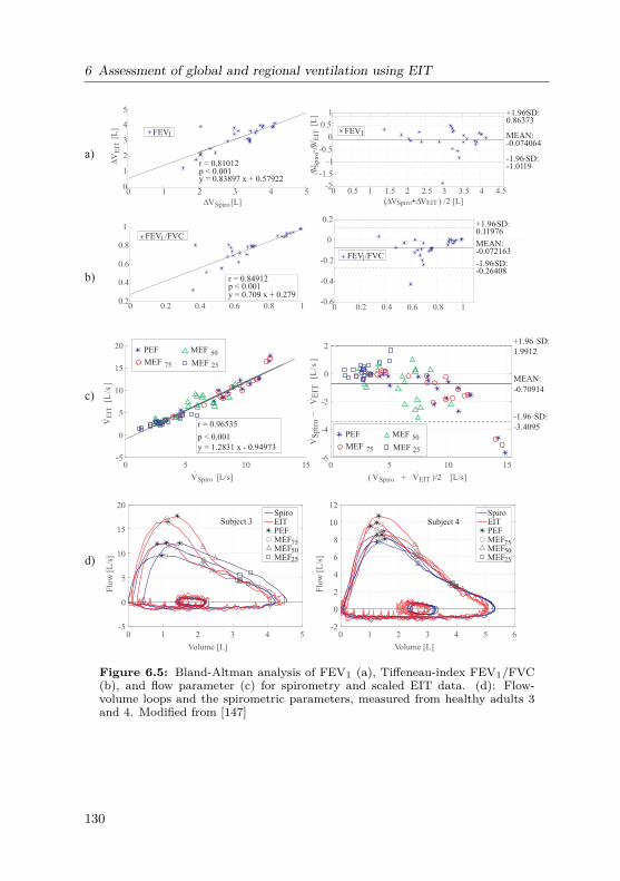
6 Assessment of global and regional ventilation using EIT
∆V [L]Spiro
∆[L
]V
EIT
∆VS
pir
o-∆
V[L
]E
IT
(∆VSpiro+∆V ) /2 [L]EIT
0 0.5 1 1.5 2 2.5 3 3.5 4 4.5-2
-1.5
-1
-0.5
0
0.5
1 +1.96·SD:0.86373
-1.96·SD:-1.0119
MEAN:-0.074064
0 1 2 3 4 50
1
2
3
4
5
r = 0.81012p < 0.001y = 0.83897 x + 0.57922
FEV1 FEV1
0 0.2 0.4 0.6 0.8 1-0.6
-0.4
-0.2
0
0.2+1.96·SD:0.11976
-1.96·SD:-0.26408
MEAN:-0.072163
0 0.2 0.4 0.6 0.8 10.2
0.4
0.6
0.8
1
r = 0.84912p < 0.001y = 0.709 x + 0.279
FEV /FVC1
FEV /FVC1
0 5 10 15
VSpiro [L/s]
-5
0
5
10
15
20
VE
IT[L
/s]
r = 0.96535
p < 0.001
y = 1.2831 x - 0.94973
PEF
MEF
MEF
MEF
0 5 10 15
( VSpiro + VEIT )/2 [L/s]
-6
-4
-2
0
2
VS
pir
o−
VE
IT[L
/s]
+1.96·SD:
1.9912
-1.96·SD:
-3.4095
MEAN:
-0.70914
75
50
25
PEF
MEF
MEF
MEF75
50
25
c)
a)
b)
0 1 2 3 4 5 6
Volume [L]
-2
0
2
4
6
8
10
12
Flo
w [
L/s
]
SpiroEITPEFMEFMEFMEF
0 1 2 3 4 5
Volume [L]
-5
0
5
10
15
20
Subject 3 Subject 4
75
50
25
SpiroEITPEFMEFMEFMEF
75
50
25d)
Flo
w [
L/s
]
Figure 6.5: Bland-Altman analysis of FEV1 (a), Tiffeneau-index FEV1/FVC(b), and flow parameter (c) for spirometry and scaled EIT data. (d): Flow-volume loops and the spirometric parameters, measured from healthy adults 3and 4. Modified from [147]
130

6.1 Diagnosis of pulmonary function with EIT during forced expiratory maneuvers
smaller and the process is slower than during a forced expiration maneuver.Since the reconstruction matrix used in the present study is based on a linearapproach developed for normal tidal volumes, a more precise reconstructionalgorithm might increase the accuracy of the EIT signals. Other nonlinear as-pects such as the change in thorax circumference, the position of the electrodes,and the position of the tissue and respiratory muscles may be considered inthis approach. Second, during a forced expiration maneuver, the respiratorymuscles contract maximal, the intra-thoracic pressure increases rapidly. As aresult, the venous return is reduced and the cardiac output is increased instan-taneously. The reduction in the intra-thoracic blood volume causes a furtherdisturbance in the measured EIT signals. More experiment should be set upto clarify these hypotheses.
The use of Tiffeneau-index and positive BSL in discriminating asthma Inasthmatic patients, all lung function parameters increased after BSL. FVCincreased from 2.37± 0.92 to 2.42± 0.93, and FEV1 from 2.16± 0.83 (2.24±0.85 by EIT) to 2.29± 0.86 (2.36± 0.89 by EIT). This resulted in a positivebronchodilator index ∆FEV1[%] = 7.44±12.94 (4.79±12.93 by EIT). Positiveeffects of BSL on the asthmatic patients were also documented in MEF75,MEF50, and MEF25.The results of the binary classification tests on the Tiffeneau-index and the
bronchodilator index are presented in Fig. 6.8, considering spirometry as thegold standard. For the Tiffeneau-index, the data were split into two groups, i.e. children over and below 12 years of age regarding the different criteria forpathological asthma [1]. The binary classification test yields high sensitivity in∆FEV1 (86.67%) and low sensitivity in TI (25% and 35.29%). High specificities(> 93%), high positive predictive value (≤ 75%) and high negative predictivevalue (> 80%) can be observed in all three criteria. No significant differencesbetween the two groups of age is documented.Since the FV loops of the asthmatics exhibit typical concave forms [133], a
graphical comparison of these loops in the asthmatics and controls is clinicallyuseful. However, since a large number of our pediatric patients were undermedical treatment and hence, exhibited normal pulmonary function values, agraphical comparison of n=58 would not demonstrate the discriminative powerof EIT between healthy and asthmatic FV loops. A better comparison will bebetween n=10 patients (3 under 12 years old and 7 over 12 years old) who hadconfirmed pathological asthma (reduced TI index and positive bronchodilatortest) with selected age-matched controls. Figure 6.9 illustrates the mean FVloops of these 10 patients (divided into two groups of different ages) and thecontrols in the same diagrams.
131

6 Assessment of global and regional ventilation using EIT
Spirometry EIT
asthma0
1
2
3
4
5
FE
V1
(L)
0
1
2
3
4
FE
V05
(L)
before BSLcontrol asthma
after BSL
r = 0.989p < 0.001r = 0.982
p < 0.001r = 0.986
p < 0.001r = 0.941
p < 0.001r = 0.905
p < 0.001r = 0.965
asthmabefore BSL
control asthmaafter BSL
0
2
4
6
8
10
12
14
16
18
20
0
1
2
3
4
5
0
2
4
6
8
10
12
ME
F (L
/s)
50
asth
ma
before BSLcontrol asthma
after BSL
asthmabefore BSL
control asthmaafter BSL
asthmabefore BSL
control asthmaafter BSL
ME
F (L
/s)
75
ME
F (L
/s)
r = 0.805p < 0.001r = 0.772
p < 0.001r = 0.849
p < 0.001r = 0.673
p < 0.001r = 0.6
p = 0.0038r = 0.374 r = 0.792
p < 0.001r = 0.689
p < 0.001r = 0.774
25
Figure 6.6: Box and whiskey plot index [143]. Data obtained from n = 58controls and n=58 asthmatics before and after BSL.
132

6.1 Diagnosis of pulmonary function with EIT during forced expiratory maneuvers
0 1 2 3 4 5 6 7 80
2
4
6
8
10
12
14
16
18
20
0 1 2 3 4 5 6 7 80
2
4
6
8
10
12
14
MEF75 MEF50 MEF25
0 1 2 3 4 5 6 7 8 9 10-12
-10
-8
-6
-4
-2
0
2
4
68
2.6131
-4.4538
MEAN:-0.92035
Vspiro
( Vspiro + VEIT )/2
-1.96 ·SD:
0 2 4 6 8 10 12-14
-12
-10
-8
-6
-4
-2
0
2
4
2.7837
-5.1769
MEAN:-1.1966
+1.96·SD:
+1.96·SD:
-1.96 ·SD:
MEF75 MEF50 MEF25
MEF75 MEF50 MEF25
MEF75 MEF50 MEF25
( Vspiro + V )EIT
Before BSL
VS
pir
o−
VE
ITV
Spir
o−
VE
IT
VE
ITV
EIT
(L/s
)
p < 0.001
r = 0.680
p < 0.001
r = 0.772
After BSL
(L/s
)
(L/s
)(L
/s)
(L/s)
(L/s) (L/s)(L/s)
Vspiro (L/s)(L/s)
Figure 6.7: Bland-Altman plot. Data obtained from n=58 controls and n=58asthmatics before and after BSL.
6.1.4 Regional EIT-derived flow volume (FV) loop
An EIT scan displays a 32x32-pixel image at one time instance. To investigateregional characteristics, each tomogram was divided into four quadrants, i.e.right dorsal (RiDo), right ventral (RiVe), left dorsal (LeDo), and left ventral(LeVe) with 16x16 pixels each. By summing up the temporal impedance changeof the pixel for each quadrant, regional impedance indexes can be calculated, e.g. ∆ZRiDo =
∑i∈RiDo∆Zi(t) [107]. Figure 6.10 illustrate global and regional
FV loops of three representative asthmatic patient (I-III). The deviation be-tween the spirometric and EIT-derived global FV loops at maximal flow canbe observed. The regional FV loops confirm positive BSL. The effect of BSLis inhomogeneous among the lung quadrants: Larger positive bronchodilatoroccurs in left dorsal and right ventral lung quadrants.It should be noted that there is no existing reference for the regional lung
133

6 Assessment of global and regional ventilation using EIT
0.6 0.7 0.8 0.9
0.6
0.7
0.8
0.9
1
Tiffeneau index (Spirometry)
Tif
fen
eau
in
dex
(E
IT)
Tiffeneau index (Spirometry)
Tif
fen
eau
in
dex
(E
IT)
0.6
0.7
0.8
0.9
1
0.6 0.7 0.8 0.9 1
Asthma before BSL Asthma after BSLControl
Age < 12 years old, FEV /FVC < 90%1
n = 35 x 3
TP = 1 FP = 0 PPV = 100
FN = 3 TN = 101 NPV = 97.12
Sensitivity = 25 Specificity = 100
n = 23 x 3
TP = 6 FP = 2 PPV = 75
FN = 11 TN = 50 NPV = 81.97
Sensitivity = 35.29 Specificity = 96.15
Age 12 years old,≥ FEV /FVC < 80%1
Asthma before BSL Asthma after BSLControl
-15 12 35 60-15
12
35
65
90
∆F
EV
[%]
(EIT
)1
∆FEV [%] (Spirometry)1
n = 58
TP = 13 FP = 3 PPV = 81.25
FN = 2 TN = 40 NPV = 95.24
Sensitivity = 86.67 Specificity = 93.02
∆
Figure 6.8: Binary classification test for TI and bronchodilator index [143].Top: FEV1/FVC < 80% for n = 35 x 3 children ≤ 12 years old (control, asthmabefore and after BSL). Center: FEV1/FVC < 90% for n = 23 x 3 children <12 years old (control, asthma before and after BSL). Bottom:∆FEV1[%] > 12for n = 58 asthmatic children. TP = true positive, FP = false positive, TN =true negative, FN = false negative, PPV = positive predictive value, NPV =negative predictive value.
function for this group of children. Non-invasive radiological technique, e.g. hyper-polarized He-magnetic resonance imaging, was not performed dueto non-availability and ethical reasons. Thus, quantitative evaluation and in-terpretation of the results depicted in Fig.6.10 is difficult. However, our re-
134

6.1 Diagnosis of pulmonary function with EIT during forced expiratory maneuvers
0 1 2 3 4 5volume (L)
-5
0
5
10
15
flow
(L
/s)
3 indi. FV loops before and after BSL
average FV loop before and after BSL
1
2
3
0 0.5 1 1.5volume (L)
-2
-1
0
1
2
3
4
5
flow
(L
/s)
0 0.5 1 1.5 2 2.5 3 3.5volume (L)
-5
0
5
10
15
flow
(L
/s)
aver. asthm. before BSL aver. asthm. after BSL aver. controls
aver.
Age 12≥ Age < 12
Figure 6.9: Top: three individual FV loops before and after BSL. An increasein FVC after BSL can be observed in all individual FV loops. Bottom: averageFV loops lung healthy controls (black, dotted), asthmatics before (blue, drawn)and after (red, drawn) BSL [143]. Selection criteria for asthmatics: left: n = 3≤ 12 years of age, TI < 0.8, ∆FEV1 > 12% , right: n = 7 < 12 years of age, TI< 0.9, ∆FEV1 > 12%.
sults demonstrate the usability of EIT to monitor not just regional ventilationchanges in diagnostic procedure, but also to determine efficacy of local drugeffects for therapy.
135

6 Assessment of global and regional ventilation using EIT
0 0.2 0.4 0.6
-0.5
0
0.5
1
1.5
0 0.2 0.4 0.6
0 0.2 0.4 0.6
-0.5
0
0.5
1
1.5
0 0.2 0.4 0.6
0 0.2 0.4 0.6 0.8-1
-0.5
0
0.5
1
1.5
0 0.2 0.4 0.6 0.8
0 0.2 0.4 0.6 0.8-1
-0.5
0
0.5
1
1.5
0 0.2 0.4 0.6 0.8
0 0.5 1 1.5
-1
0
1
2
3 RiVe
0 0.5 1 1.5
LeVe
0 0.5 1 1.5
-1
0
1
2
3RiDo
0 0.5 1 1.5
LeDo
flow
[l/
s]fl
ow
[l/
s]
volume [l] volume [l]
RiVe LeVe
RiDo LeDo
flow
[l/
s]fl
ow
[l/
s]
volume [l] volume [l]
flow
[l/
s]fl
ow
[l/
s]
volume [l] volume [l]
RiVe LeVe
RiDo LeDo
10Spiro before BSLSpiro after BSLEIT before BSLEIT after BSL
Spiro before BSLSpiro after BSLEIT before BSLEIT after BSL
Spiro before BSLSpiro after BSLEIT before BSL
ReferenceEIT after BSL
Spiro before BSLSpiro after BSLEIT before BSL
ReferenceEIT after BSL
Reference
I
II
III
Figure 6.10: Spirometric and EIT-derived FV loop of one representative asth-matic patient. Left: global FV loops, right: regional FV loops obtained fromEIT images for right ventral (RiVe), left ventral (LeVe), right dorsal (RiDo), andleft dorsal (LeDo) quadrant of the lung. [143].
136

6.2 Introduction of oscillatory Electrical Impedance Tomography (oEIT)
6.2 Introduction of oscillatory Electrical ImpedanceTomography (oEIT)
The use of EIT in the Tiffeneau-Test for regional lung functions is not suited forinfants, young children, and patients with serve lung damages, since the forcedexpiration maneuvers requires strong patients’ cooperation. In this section, weinvestigate a new measurement modality to assess regional lung mechanics bycombining EIT and FOT. The new technique is named oscillatory electricalimpedance tomography (oEIT).The measurement system of oEIT, illustrated in Fig. 6.11, consists of an
FOT device, a flow and pressure sensor system, and an EIT device. TheFOT measurements were performed as described in Chapter 4. Simultaneously,EIT frames were generated with the PulmoVista 500. Measurements wereperformed on n= 5 healthy volunteers (four male, one female, age between 23and 55). Subjects were asked to perform an apnea for 10s, followed by normalbreathing.
EITDevice
Computer
Bacteria filterFOT
aoP (t)
V (t).
Device
ao
Figure 6.11: The oEIT measurement system [149].
6.2.1 Visibility of FOT frequencies in EIT signal
∆Zeit(t,5Hz) and its derivative d∆Zeit(t,5Hz)/dt on a exemplary measurementat fos = 5Hz are depicted in Fig. 6.12. In the apnea phase, ∆Zeit(t,5Hz)remains unchanged except of small cyclic perturbations at heart rate. The5Hz-oscillations are visible in the derivative d∆Zeit(t,5Hz)/dt. The resultsindicate the visibility of the FOT frequency in the EIT response.Fig. 6.13 presents a representative magnitude of the Fourier transforms
computed for VoEIT(t) measured with EIT. VoEIT contains three groups of
137
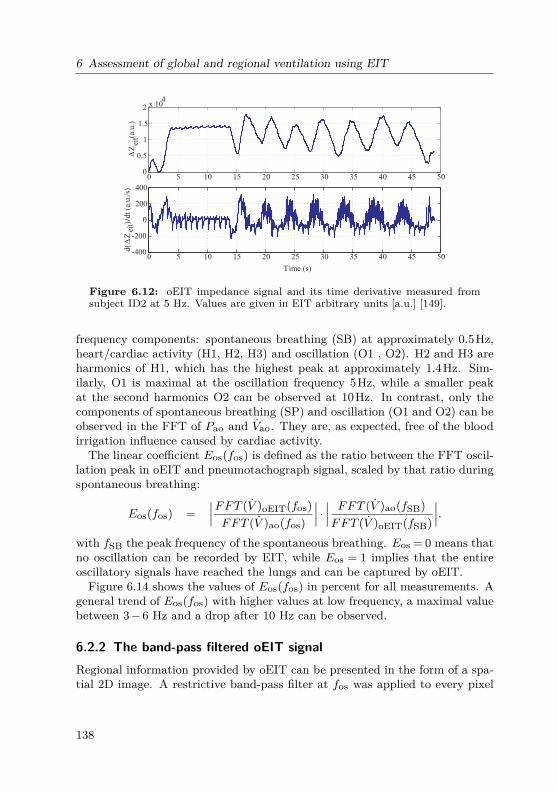
6 Assessment of global and regional ventilation using EIT
0 5 10 15 20 25 30 35 40 45 500
0.5
1
1.5
2 x 10⁴
∆Z
(a
.u.)
eit
0 5 10 15 20 25 30 35 40 45 50-400
-200
0
200
400
Time (s)
d(∆
Zei
t)dt
(a.u
./s)
/
Figure 6.12: oEIT impedance signal and its time derivative measured fromsubject ID2 at 5 Hz. Values are given in EIT arbitrary units [a.u.] [149].
frequency components: spontaneous breathing (SB) at approximately 0.5Hz,heart/cardiac activity (H1, H2, H3) and oscillation (O1 , O2). H2 and H3 areharmonics of H1, which has the highest peak at approximately 1.4Hz. Sim-ilarly, O1 is maximal at the oscillation frequency 5Hz, while a smaller peakat the second harmonics O2 can be observed at 10Hz. In contrast, only thecomponents of spontaneous breathing (SP) and oscillation (O1 and O2) can beobserved in the FFT of Pao and Vao. They are, as expected, free of the bloodirrigation influence caused by cardiac activity.The linear coefficient Eos(fos) is defined as the ratio between the FFT oscil-
lation peak in oEIT and pneumotachograph signal, scaled by that ratio duringspontaneous breathing:
Eos(fos) =∣∣∣FFT (V )oEIT(fos)FFT (V )ao(fos)
∣∣∣ · ∣∣∣ FFT (V )ao(fSB)FFT (V )oEIT(fSB)
∣∣∣.with fSB the peak frequency of the spontaneous breathing. Eos = 0 means thatno oscillation can be recorded by EIT, while Eos = 1 implies that the entireoscillatory signals have reached the lungs and can be captured by oEIT.Figure 6.14 shows the values of Eos(fos) in percent for all measurements. A
general trend of Eos(fos) with higher values at low frequency, a maximal valuebetween 3−6 Hz and a drop after 10 Hz can be observed.
6.2.2 The band-pass filtered oEIT signalRegional information provided by oEIT can be presented in the form of a spa-tial 2D image. A restrictive band-pass filter at fos was applied to every pixel
138

6.2 Introduction of oscillatory Electrical Impedance Tomography (oEIT)
0 2 4 6 8 10 12 14 16 18 200
0.05
0.1
0.15
0.2
0.25
FF
TV
ao(L
/s)
0 2 4 6 8 10 12 14 16 18 200
0.1
0.2
0.3
FF
TV
oE
IT(L
/s)
SB H2H1 O1H3 O2
Frequency (Hz)
[cm
H O
]2
..
FF
TP
ao
0 2 4 6 8 10 12 14 16 18 20
0.5
1
0
Figure 6.13: Fast Fourier transform of VoEIT, Vao and Pao. fos = 5 Hz [149].Components: SB = spontaneous breathing, H = heart, O = oscillation.
0
20
40
60
80
100
0 5 10 15 20
ID1 ID2 ID3 ID4 ID5 Average
E(f
)
(%
)os
os
Frequency (Hz)
Figure 6.14: The coefficient Eos(fos) in percent [149].
∆zoEIT(i, j,fos) to exclude any cardiac or spontaneous breathing activity. Theband-pass filtered oEIT images have the same orientation of unfiltered EITimages (Fig. 6.15). Fig. 6.15 also depicts three random consecutive oscilla-tory cycles for bandpass-filtered oEIT volume and flow. The signals consistof sinusoidal oscillation with a period of Tos = 0.2s. Each period includes 10
139

6 Assessment of global and regional ventilation using EIT
dorsal
ventral
right
dorsal
ventral
right
ventralBandpass-filtered
∆zoEIT-Filtered(i, j, fos )∆zoEIT (i, j )
left left
classical EITimage Bandpass-filtered oEITimage
-1 -0.5 0 0.5 1
-1 -0.5 0 0.5 1
Tim
e/s
Oscillation Cycle
v1
v2
v3
v4
v5
v6
v8
v7
v9
v10
f1
f2
f3
f4
f5
f6
f8
f7
f9
f10
Cycle 2Cycle 1 Cycle 1Cycle 3 Cycle 3Cycle 2
v1
0
0.02
0.04
0.06
0.08
0.2
0.14
0.12
0.16
0.18
0.1
d z∆oEIT-Filtered
( i, j, fos )/dt∆z
oEIT-Filtered( i, j, fos )
Figure 6.15: Top: Orientation of the band-pass filtered oEIT images. Bottom:oEIT volume (left) and flow (right) during three oscillatory cycles. From [149]
140

6.3 Summary
images numbered from 1 to 10. ∆zoEIT(i, j,fos) are shown on the left side (v1-v10) and the derivative d∆zoEIT(i, j,fos)/dt on the right side (f1-f10), wherefi = vi+1−vi, i= 1..10. Each oscillatory cycle starts at low lung volume (v1),reaches the maximum after 5 sampling times (v5-v6), and ends at minimal lungvolume (v10). Pixels with impedance almost equal to zero were set to whiteto separate the lung and non-lung regions.Regarding the results, we hypothesize several properties of the band-pass
filtered oEIT signal:
• Band-pass filtered oEIT images have repeating patterns in several con-secutive oscillatory cycles. The images v1-v10 do not alter significantlyamong three oscillation cycles.
• Absolute value of band-pass filtered oEIT flows is fos2 -periodic. The im-
ages f1, f2, f3, f4, f5 are almost equal to f6, f7, f8, f9 and f10, respectively,with a sign conversion.
• Ventilation appears to be stronger in ventral than dorsal lung regions. InFig. 6.15, ventral ventilation is stronger in oEIT volume and flow images(see v2, v3, v4, f2, f3, f4,...). The effect of the sinusoidal perturbationmight be considered as small amplitude mechanical ventilation whichcauses a stronger gas distribution in the ventral regions [152].
• A band-pass filtered oEIT cycle is observed to consist of a homogeneousand an inhomogeneous phase. Each positive or negative half cycle couldbe divided into a homogeneous phase (images f1, f2) and an inhomoge-neous phase (images f3-f5). After f3, the oEIT volume becomes left-rightinhomogeneous. The positive oEIT flows concentrates in an oval region-shaped region, while flows in other regions have already become negative.
6.3 Summary
There has been an increasing interests in the use of EIT for global and re-gional lung function diagnostics. Strict correlation of EIT impedance changeand thoracic air content has been reported in the literature for normal tidalbreathing. Our studies on healthy subjects and asthmatic pediatric patientsinvestigate this correlation for the forced expiratory maneuvers. Results showa strict linearity between global EIT and spirometric data in all parameters(FEV1,FEV0.5,MEF75,MEF50,MEF25). The EIT-derived Tiffenenau indexand the bronchodilator test index have a high potential in assessing asthma inpediatric patients. The EIT-derived mean FV loops of the asthmatic childrenyield typical concave shapes with improvement of the FV loops before and after
141

6 Assessment of global and regional ventilation using EIT
BSL. Regional lung function may be illustrated by regional FV loops obtainedby EIT for different lung regions. Further studies on regional pulmonary func-tions with EIT are needed to validate the findings, since no established goldstandard for regional lung function exists.Another method for regional pulmonary diagnostics is the novel combination
oEIT between EIT and FOT. Measurements on healthy subjects show thevisibility of FOT frequencies in the Fourier transform of the global EIT index.Optimal oEIT frequencies are between 4Hz and 10Hz. The band-pass filteredoEIT signal demonstrates the dynamic behavior of different lung regions andmight become a future tool in regional pulmonary function.
142

7 Discussion and outlook
The journey is what brings us happiness not the destination.Dan Millman
This book has accompanied us on a long journey throughout the complexphysical nature of lung mechanics and a wide range of comprehensive math-ematical descriptions and measurement methodologies. Following the goalsdefined at the beginning, various facets are comprised in this research. Start-ing with a nonlinear lumped modeling approach, the thesis continues applyingmodel-based analysis to reevaluate existing pulmonary testing methods and todevelop novel, innovative advances in respiratory measurements. Sophisticatedmodels of the lung-heart interactions including the lymphatics and the inter-stitial fluid filtration contributes to a better understanding in the systematicdevelopment of cardiopulmonary diseases.Throughout this work, miscellaneous scientific contributions have been achie-
ved. Some of them are in the center of scientific discussions in the currentstate-of-the-art. Reviewing the chapters of this book, some answers can beproposed for the discussions:
1. Are object-oriented programming languages useful for modeling of com-plex physiological systems?Yes, definitely.The use of object-oriented modeling language (OOML) in simulation oftechnical systems is not a new approach. In 2008, Mathworks releasedthe first Simscape version in their R2008a+ product. Object-orientedapplications in the fields of biophysical and medical systems came laterand are still moderate. Only a few publications can be found whichuse OOML to model biophysical systems: Brunberg 2009 (Dymola) [24],Barnea 2010 (Matlab Simpower) [7], de Canete 2013 (Simscape) [36],Heinke 2015 (Dymola) [77]. The models introduced in this research arethe most comprehensive OOML model of the cardiorespiratory mechan-ics so far. The OOML Simscape™ exhibits the following significant ad-vantages over more "traditional" modeling tools (Fortran, C++, MatlabSimulink™):
• The graphical implementation of complex model structure in OOMLis intuitive for developers. In text-based programming language, theengineer has to deal with a great amount of equations which explodesfor complex systems. More detailed comparisons between the causal(text-based, signal-oriented) and acausal modeling (OOML) are dis-cussed in [36,99]. In OOML, the implementation of constitutive and
143
7 Discussion and outlook
phenomenological equations are "decentralized", i.e. coupled witha graphical component, and no explicit implementation of balanceequations is needed. The meaning of the components in a graphicalmodel is directly understandable.
• OOML can connect subsystems bi-directionally as in the real physi-cal world. This was demonstrated with the interconnection betweenthe respiratory and cardiovascular system in our model. While car-diopulmonary models published by other authors consider an uni-directional between these systems, i.e. the changes in cardiovascularblood pressures and volume regarding in- and expiration [3,89,117],our model describes the interactions in both directions, for examplethe development of cardiogenic pulmonary congestion.
2. Are nonlinear multi-compartment models of lung mechanics recommendedfor off-line or even real-time applications in respiratory care?Yes, perhaps.In most applications in respiratory care, the respiratory system are ap-proximated by a simple resistance-compliance model [111]. This simplifi-cation has become a standard description in all physiological and medicaltextbooks [68, 96]. However, this model structure is too simple to ade-quately present the highly non-linear mechanics of the lungs. It is obviousthat with only two parameter Rrs and Crc, descriptions of pathologicalconditions are very limited.The respiratory model introduced in Chapter 3 has demonstrated itsability to model more complex nonlinear behaviors of the lungs. Thecompartmentalization ensures an equivalent between mathematical de-scription and physiological interpretation. It should be noted that thedeveloped model demonstrates the first use of OOML in analysis andevaluation of respiratory mechanics, as shown for the interrupter tech-nique in Chapter 3.Multi-compartment modeling yields more possibilities in interpretationof measurement data regarding physiological equivalent and possible dis-turbances. Furthermore, since the simulation in Simscape™ is more thanten times faster than in real-time, model-based online monitoring and de-cision support can be considered as potential applications of the modelin future research.
3. Is there a clear physiological and physical coherence between the respira-tory parameters measured with different pulmonary testing method, suchas body plethysmography, interrupter, and forced oscillation technique?
144
With high probability.In the current state-of-the-art, the coherence between the parameter ob-tained with the body plethysmography (Raw), the interrupter technique(Rint), and the forced oscillation technique at different frequencies (R5,R20, Z(jω)) is not clearly addressed. Clinical studies showed correlationamong the value of these parameter in presence of pathologies, however,did not focus on the underlying physiology. The model-based analysisdiscussed in Chapter 3 and Chapter 4 proposes clear correspondencesbetween the compartments and the measurement techniques. The inter-rupter resistance Rint comprises the airway resistance Raw and chest walldamping Rcw.
4. Does model-based parameter identification provide additional diagnosticinformation beside the respiratory impedance measured with FOT? Andif yes, which models should be used?Yes and no.Recently, an interesting discussion on the use of the respiratory impedanceZ(jω) in pulmonary function testing and lung monitoring has been car-ried out by world leading scientists in lung mechanics [8]. The maindiscussion was between Bates, who supported the use of Z(jω) in re-lation with the constant-phase model and Mitzner, who questioned thecontribution of Z(jω) in clinical praxis. The discussion indicated that theinterpretation of G and H in the constant-phase model estimated withZ(jω) is not persuasive to describe the changes in lung mechanics duringpathological conditions. Unfortunately, Mitzner and Bates focused theirdiscussion only on the constant-phase model (which they considered asthe newest, most advanced model) and did not consider the Mead model.Our model-based analysis with the step-by-step model simplification haspointed out, that the RIC, eRIC, aRIC, and visco-elastic models are sim-plification of the Mead model. Indeed, the Mead model presents thebest correspondence to lung physiology, while the constant-phase andDuBois’s models overestimate the influence of lung tissue damping.The results of this research support the use of the eRIC model for normalFOT, aRIC model for FOT including frequencies above 20 Hz, and thev-eRIC+ model for volume-dependent FOT measurements.
5. Is the object-oriented cardiopulmonary model able to reproduce the sys-tem behaviors physiologically during various scenarios from spontaneousbreathing to mechanical ventilation?Yes, it is.The object-oriented model of the cardiopulmonary interactions was val-
145
7 Discussion and outlook
idated for spontaneous breathing, the Mueller maneuver, and differentmechanical ventilation modes. In most cases, model behaviors correlatewell with clinical and animal data. It should be noted again that modelparameters remained constant during all simulation, i.e no parameterestimation and adaption was performed to fit the data.The model does not include the cardiac and respiratory regulation, thus,is almost completely passive in its current form. All of the componentsexcept the driver functions are passive elements (resistance, compliance,diodes, inertance). Simulation results have suggested that the passiveintrathoracic pressure as a mechanical coupling between the cardiovas-cular and respiratory system has an important role in cardiopulmonaryinteractions.
6. Are the lymphatics and the fluid balance system successfully modeled?Likely.There is a lack of understanding the physiological functionality of thelymphatics, and also a lack on animal and clinical data of the lymphs. Asa first pilot simulative study, a comprehensive extension of the model wasconsidered. The respiratory system was coupled with the cardiovascularsystem over the lymphatics. Simulation results have demonstrated theexpected behaviors of the lymph, the fluid filtration and re-absorptionduring the development of cardiogenic edema and the effect of CPAPtherapy. Similar simulations can be used to design future clinical studyfor a better understanding of the lymphatics and thoracic fluid balance.
7. How much potential does Electrical Impedance Tomography have as afuture tool for online monitoring and assessing of global and regional lungmechanics?Very high potential.Existing lung function methods are restricted to global information. Bycontrast, the Electrical Impedance Tomography provides a non-invasivetool to assess regional dynamic functionality of lung mechanics. Thisresearch presents the novel use of the EIT-derived flow-volume loop indiagnosing of asthma in pediatric patients. Linearity between EIT andspirometry was reported in adults and children with a slight deviationat the maximum flow. This research also proposed a novel combinationbetween EIT and FOT and demonstrates the visibility of high frequencycomponents in the EIT signal. Combination between EIT and othermeasurement modalities such as body plethysmography and interruptertechnique, as well as a large clinical study for oEIT should be consideredin future researches.
146

A Appendix
A.1 Non-linear parameter identification using Least Squaresfitting
Least Squares is a standard method in regression analysis to estimate the solu-tion of overdetermined equation systems. It minimizes the sum of the squaresof the residuals between data and model. The sum of the squares error S isgiven as:
S =n∑i=1
r2i =
n∑i=1
(yi−f(xi,θ))2 = ‖y−f‖22 . (A.1)
ri is the error between data yi and model f(xi,θ) for the i-th model equation.The vectors y ∈ Rn, f ∈ Rn and θ ∈ Rm present the measurement data, themodel outputs, and the parameters. The Least Squares method is generally aminimization problem minθ ‖y−f‖22.For parameter estimation of lung mechanics in the frequency domain, a non-
linear Least-Squares fitting can be applied. The estimation problem can bewritten as:
minθ‖Zmeas−Zmodel‖22 = min
θ
∥∥∥∥( ZR,meas−ZR,modelZX,meas−ZX,model
)∥∥∥∥2
2(A.2)
= minθ
∥∥∥∥∥∥∥∥∥∥∥∥∥
ZR,meas(ω1,θ)−ZR,model(ω1,θ)...
ZR,meas(ωn,θ)−ZR,model(ωn,θ)ZX,meas(ω1,θ)−ZX,model(ω1,θ)
...ZX,meas(ωn,θ)−ZX,model(ωn,θ)
∥∥∥∥∥∥∥∥∥∥∥∥∥
2
2
,
with the impedance vectors Zmeas, Zmodel ∈Cm×(2n), the resistive impedancevectorZR,meas, ZR,model ∈Rm×n, and the reactance vectorsZX,meas, ZX,model∈Rm×n. m is the number of data points, and n is the number of the measuredFOT frequencies ω.A non-linear fitting can be performed with the Matlab function lsqnonlin,
which is based on an upper and a lower limit of the parameters to be identifiedon a trust-region-method [34]. The numerical solution for minimizing the errorby the trust region method is not a global but a local minimum. The non-linearfunction to be minimized is approximated by a quadratic function. Because of
147

A Appendix
the trust region method, this approximation only takes place locally near theiterations of the parameter vector. Hence, for the identification of respiratoryparameters, the choice of initial values of the parameter vector is an importantissue.
A.2 Reynold number, flow patterns, and Hagen-Poiseuille’slaw
In 1883, Reynolds examined patterns of flow by injecting ink into a waterstream through a pipe [185]. He found that flow could be described by twodifferent categories depending on its velocity: laminar and turbulent flow. Thisclassification is not only valid for fluids, but air flow can be divided into laminarand turbulent flow as well. An important figure in characterizing flow is thedimensionless Reynolds number Re, which is calculated as follows:
Re = vd
ν= V d
Aν, (A.3)
where d is diameter and A is cross-sectional Area of a circular pipe. Re isdependent on the properties of the passed pipe, the physical properties of thefluid and the flow rate. If the shape of the pipe and the flowing fluid areknown, Re is linearly dependent on the flow rate and thus, can be employed asa classification figure for flow regimes.Laminar flow is characterized by a regular, ordered flow pattern [185]. Fig.
A.1(a) illustrates the laminar airflow in the main direction of flow with aparabolic velocity profile. Laminar flow is found for low flow rates and forRe 2100 in circular pipes. For laminar flow, pressure is connected to flow ina linear relationship:
∆P (t) =KV (t) = 8µLπr4 V (t) , (A.4)
where K is a constant [70], which, for circular tubes, can be expressed byphysical properties of the fluid (or gas) and the length L and the radius r ofthe tube. This relation is known as Hagen-Poiseuille’s law [87]. K correspondsto the laminar flow resistance of a pipe:
Rlaminar = 8µLπr4 . (A.5)
For increasing flow rates, air (or fluid) movements become turbulent. Fig.A.1(b) shows the flow pattern for turbulent flow. The regular flow patterns areabandoned by the addition of random fluctuations superimposed on the velocity
148

A.2 Reynold number, flow patterns, and Hagen-Poiseuille’s law
Figure A.1: Patterns for different flow regimes.
component in direction of flow [185] and air moves chaotically. The irregularmovement of flow causes additional friction and the pressure-flow relationshipbecomes non-linear:
∆P (t) =KV α(t), α ∈ [1.75;2] , (A.6)
where K is a constant, [70]. In a circular pipe, turbulent flow is associatedwith Re 4000 [185].Laminar flow does not change to turbulent flow abruptly and for 2100Re
4000 flow transfers through a transition regime [185], in which both laminarand turbulent flow attributes are found. The pressure-flow relationship in thetransition regime can be described by the Rohrer equation, which is defined asfollows:
∆P (t) =K1V (t) +K2V2(t) , (A.7)
where K1 and K2 are constants. Turbulent flow resistance of a pipe is flow-dependent:
Rturbulent =K1 +K2V . (A.8)
149

A Appendix
A.3 Respiratory modeling
CRs
RrsV
Palv
Pmouth
Pmus
Cl
RrsV
PPmouth
Pmus
Ccw
Ppl
R
in
V
PalvPmouth Rrs,ex CRs
alv
Pmus
(B) R -R model(C) Lung - chest model
(A) RC model
rs,in
ex
cR RopenRconstrict
CRs
palv
Pmus
Pmouth
uawR R sRc
Ppl
Pmouth Cc
R ti
Clppl
EPP
(F) Mead_2 model
(G) Liu model
Ccw
RlV
Ppl
Pmouth
Pmus
Rtr Rb RA
CACtrCl Cb
Palv
(E) Rideout model
Figure A.2: Lung models used in mechanical ventilation (A-D), or in spirom-etry for description of flow limitation (E-F).
150

A.3 Respiratory modelingT
able
A.1
:Ana
tomical
mod
elof
thehu
man
bron
chialtree
accordingto
Weibe
l,N
=generation
numbe
r;N
b=
numbe
rof
tube
s,L
=leng
thof
tube
,d=
diam
eter
oftube
,S
=totalcross-sectiona
larea,V
b=
totalvolumeof
tube
s,∑ V b
=cumulativetube
volumeof
allg
enerations
upto
N,V
alv=
alveolar
volume,V
=totalv
olum
e,∑ V
=cumulativetotalv
olum
e[38].
NN
TL
dS
Vb
∑ V bV
alv
V∑ V
cmcm
cmcm
2cm
3cm
3cm
3cm
3cm
3
01
121.8
2.54
30.54
30.5
030.54
30.54
12
4.76
1.22
2.34
11.13
41.7
011.13
41.67
24
1.9
0.83
2.16
4.11
45.8
04.11
45.78
38
0.65
0.479
1.44
0.94
46.7
00.94
46.72
416
1.085
0.385
1.86
2.02
48.7
02.02
48.74
532
0.915
0.299
2.25
2.06
50.8
02.06
50.8
664
0.769
0.239
2.88
2.21
53.0
02.21
53.01
7128
0.65
0.197
3.88
2.52
55.5
02.52
55.53
8256
0.547
0.159
5.08
2.78
58.3
02.78
58.31
9512
0.462
0.132
6.97
3.22
61.5
03.22
61.53
101024
0.393
0.111
9.9
3.9
65.4
03.9
65.43
112048
0.333
0.093
144.65
70.1
04.65
70.08
124096
0.282
0.081
21.2
5.98
76.1
05.98
76.06
138192
0.231
0.07
31.6
7.29
83.4
07.29
83.35
1416384
0.197
0.063
51.5
10.12
93.5
010.12
93.47
1532768
0.171
0.056
8214
107.5
014
107.47
1665536
0.141
0.051
135
19.09
126.6
019.09
126.56
17131072
0.121
0.046
219
26.43
153.0
3.9
30.33
156.89
18262144
0.1
0.043
376
37.6
190.6
13.1
50.7
207.59
19524288
0.085
0.04
664
56.23
246.8
39.4
95.63
303.22
201048576
0.071
0.038
1218
86.4
333.2
138
224.4
527.62
212097152
0.06
0.037
2225
133.1
466.3
273
406.1
933.72
224194304
0.05
0.035
4045
204
670.3
551
755
1688.72
238388608
0.043
0.035
8091
345.7
1016.0
938
1283.7
2972.42
151

A Appendix
A.4 Sensitivity analysis of the Mead’s model
0 5 10 15 20 25 30 35 402
4
6
8
10
12
14
00.010.11234689
0 5 10 15 20 25 30 35 40-7
-6
-5
-4
-3
-2
-1
0
1
0.010.11234689
0 5 10 15 20 25 30 35 40-2
-1.5
-1
-0.5
0
0.5
1
0 5 10Frequency (Hz)
20 25 30 35 402
4
6
8
10
12
14
16
0123456789
0 5 10 15 20 25 30 35 402
2.5
3
3.5
4
4.5
5
00.0010.0020.0050.0080.0090.010.0120.0150.017
15
Z (
cmH
O/L
/s)
2R
R = +2 cmH O/L/s2∆R ( ); ∆R = 0 - 9c cc
Frequency (Hz)
Z (
cmH
O/L
/s)
2R
R = 3 + ∆R (cmH O/L/s); ∆R = 0 - 92p pp
0
Z (
cmH
O/L
/s)
2X
R = 3 + ∆R (cmH O/L/s); ∆R = 0 - 92p pp
Frequency (Hz)
C = 0.04 + ∆C (L/cmH O); ∆C = 0 - 0.0172b bb
Z (
cmH
O/L
/s)
2R
C = 0.04 + ∆C (L/cmH O); ∆C = 0 - 0.0172b bb
R c
R p
R p
C b C b
R c
Z (
cmH
O/L
/s)
2R
00.0010.0020.0050.0080.0090.010.0120.0150.017
Figure A.3: Sensitivity analysis of the parameter Rc, Rp, and Cb of the Mead’smodel.
152
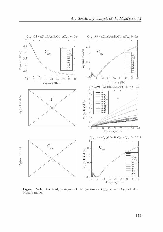
A.4 Sensitivity analysis of the Mead’s model
0 5 10 15 20 25 30 35 40-1.5
-1
-0.5
0
0.5
1
00.010.020.050.10.20.30.40.50.6
0 5 10 15 20 25 30 35 40-1.5
-1
-0.5
0
0.5
1
00.010.020.050.10.20.30.40.50.6
0 5 10 15 20 25 30 35 40-2
0
2
4
6
8
10
12
1400.0010.0020.0040.0050.0060.010.020.030.04
0 5 10 15 20 25 30 35 402
2.5
3
3.5
4
4.5
5
00.010.020.050.10.20.30.40.50.6
Z (
cmH
O/L
/s)
2R Z
(
cmH
O/L
/s)
2X
Z (
cmH
O/L
/s)
2X
Z (
cmH
O/L
/s)
2X
C = 0.3 + ∆C (L/cmH O); ∆C = 0 - 0.62alv alv alv C = 0.3 + ∆C (L/cmH O); ∆C = 0 - 0.62alv alv alv
Frequency (Hz) Frequency (Hz)
Frequency (Hz)
I = 0.004 + ∆I (cmH O/L/s²); ∆I = 0 - 0.042
Frequency (Hz)
C = 3 + ∆C (L/cmH O); ∆C = 0 - 0.0172cw cw cw
Calv
Calv
Ccw
II
Ccw
Z (
cmH
O/L
/s)
2R
Z (
cmH
O/L
/s)
2R
Figure A.4: Sensitivity analysis of the parameter Calv, I, and Ccw of theMead’s model.
153

A Appendix
A.5 Parameter of the cardiovascular model
A.5.1 Heart
Driver functions of atria, ventricles and septum:
ela,ra(t) =Aa ·e− 0.5
B2a·( HR
80 )2·(t−Ca· 80HR )2
elvf,rvf(t) =4∑i=1
Ai ·e− 0.5
B2i
·( HR80 )2·(t−Ci· 80
HR )2
+D
esept(t) = elvf(t) (A.9)
A, B, and C are the Gaussian magnitude, width, and delay, respectively [153].HR is the heart rate. D is a baseline/offset which prevents the ventricularpressure from reaching negative values. D is equal 0.02 for the left and 0.07for the right ventricle.
0 0.2 0.4 0.6 0.80
0.2
0.4
0.6
0.8
1
1.2
Time (s)
e(t)
0 0.2 0.4 0.6 0.80
0.2
0.4
0.6
0.8
1
1.2
Time (s)
e(t)
Driver function right ventricleDriver function left ventricle
Figure A.5: Left and right ventricular driver functions.
Param. Units i= 1 i= 2 i= 3 i= 4Av,i – 0.43 0.36 0.5 0.55Bv,i s 0.045 0.035 0.037 0.036Cv,i s 0.175 0.23 0.275 0.3Aa – 0.9 – – –Ba s 0.018 – – –Ca s 0.065 – – –
154

A.5 Parameter of the cardiovascular model
ESPVR and EDPVR of four heart chambers and septum:
Pes = Ees · (V −Vd)
Ped = P0 · (eλ(V−V0)−1)P (V,t) = e(t) ·Pes(V ) +(1−e(t)) ·Ped(V )
Pressure-volume relationship of the pericardium:
Ppcd(t) = P0,pcd(eλpcd(Vpcd(t)−V0,pcd)−1)
Volume balance equations:
Table A.2: Parameters of the heart model.Param. P0 V0 Vd λ Ees
Units cmH2O mL mL L−1 cmH2OL−1
la 1.1236 0 20 60 294.27ra 1.1236 0 20 50 217.53lvf 0.0926 20 15 33 3573.7rvf 0.211 20 5 23 895.5sept. 1.5096 2 2 435 66303peri. 0.068 260 – 30 –
Vlvf = Vlv−VsptVrvf = Vrv +Vspt
Vlv = Vlvf +Vspt
Vrv = Vrvf −Vspt
Vpcd(t) = Vla(t) +Vlv(t) +Vra(t) +Vrv(t)
A.5.2 Pulmonary and systemic circulationVeins
Normal veins:V = 1
λ· log(Ptm + P0) +V0 (A.10)
Collapsed veins:if V <= Vclp
155

A Appendix
V = 0.2 ·Vclp · tanh( 5Vclp·λ·(Pclp+P0) · (P −Pclp)) +Vclp
Pclp = eλ(Vclp−V0)−P0where Vclp is a threshold volume of collapsed veins.
Table A.3: Parameters of the veins.Param. P0 V0 Vclp λ
Units cmH2O L L L−1
Syst. veins 6.328 1.8456 1.25 1.8361Pulm. veins -3.567 0.0895 0.0625 10
Pulmonary capillaries
Pulmonary capillaries compliance:
V = V0 + 1λ· tanh(c ·Ptm + P0) (A.11)
Pulmonary capillaries resistance:
R= R1 ·(V1−0.9Vmin)2
(Vt−0.9Vmin)2 (A.12)
Parameters of the pulmonary capillaries are given in Table 5.2. The systemiccapillaries are included in the systemic arteries.
Arteries
The pressure-volume characteristics of pulmonary and systemic arteries:
V −Vd = Ptm ·C (A.13)
Table A.4: Parameters of the arteries.Param. C VdUnits L/cmH2O LSyst. arteries 0.0011 0.6Pulm. arteries 0.0022 0.1
156

A.6 Exemplary Simscape code of a model component
A.6 Exemplary Simscape code of a model component
The following Simscape code presents the non-linear resistance of the peripheralairways. A component belongs to a domain (in this case electrical.branch) andcontains parameters, inputs, outputs, and equations. It should be distinguishedbetween algebraic (with ’=’) and physical equations (with ’==’).
component R_vessel < foundation.electrical.branch% non-linear colapsible resistanceR1 = 1, ’Ohm’ ; % R1V1 = 0.1, ’A*s’ ; % V1Vmin = 0.05, ’A*s’ ; % VminendinputsVol = 1, ’A*s’ ; % VolumeendoutputsRout = 1, ’Ohm’ ; % R_outendequationsletR = R1*(V1-0.9*Vmin)/(Vol-0.9*Vmin);inv == R*i;Rout == R;endendend
157

AAppendixA.7 Spirometric and EIT-derived parameters
Spirometric parameters (pneumotachography)Healthy controls Asthma before BSL Asthma after BSL
Mean % ref. Mean % ref. Mean % ref.Mean ± SD pred. ± SD Mean ± SD pred. ± SD Mean ± SD pred. ± SD
FVC [L] 2.48 ± 0.93 78 ±15.9 2.37 ± 0.92 77.3 ± 15 2.42 ± 0.93 79.7 ± 14.7FEV1 [L] 2.38 ± 0.87 90.3 ± 13.7 2.16 ± 0.83 83.7 ± 16.9 2.29 ± 0.86 88.9 ± 16FEV0.5 [L/s] 1.86 ± 0.63 93.1 ± 16.9 1.64 ± 0.61 83.7 ± 20.5 1.80 ± 0.63 92.7 ±19.9MEF75[L/s] 4.62 ± 1.61 93.4 ± 18.9 4.03 ± 1.6 80.1 ± 23.3 4.63 ± 1.67 92.1 ± 21.1MEF50 [L/s] 3.5 ± 1.18 98 ± 21.6 2.75 ± 1.09 77.4 ± 23.3 3.37 ± 1.24 95.0 ± 24.6MEF25 [L/s] 2.02 ± 0.77 109.3 ± 28.7 1.52 ± 0.67 82.7 ± 28.5 1.95 ± 0.81 106.3 ± 32.4FEV1/FVC [%] 95.97 ± 4.56 115.2 ± 12.5 91.36 ± 7.62 108.8 ± 9.72 94.89 ± 5.68 112.6 ± 6.9∆FEV1 - - - - 7.44 ± 12.94 -
EIT-derived spirometry parametersHealthy controls Asthma before BSL Asthma after BSL
Mean ± SD - Mean ± SD - Mean ± SD -FVC [L] 2.48 ± 0.93 - 2.38 ± 0.92 - 2.42 ± 0.93 -FEV1 [L] 2.36 ± 0.87 - 2.24 ± 0.85 - 2.36 ± 0.89 -FEV0.5 [L/s] 1.90 ± 0.73 - 1.79 ± 0.69 - 1.90 ± 0.73 -MEF75 [L/s] 6.16 ± 2.77 - 5.24 ± 2.98 - 6.68 ± 3.51 -MEF50 [L/s] 4.23 ± 1.89 - 3.84 ± 1.78 - 4.52 ± 2.17 -MEF25[L/s] 2.25 ± 0.97 - 1.99 ± 0.92 - 2.34 ± 1.07 -FEV1/FVC [%] 95.28 ± 5.93 - 94.22 ± 5.99 - 97.73 ± 3.67 -∆FEV1 - - - - 4.79 ± 12.93 -
Table A.5: Mean values ± SD of lung function parameters, measured by spirometry and EIT on 58 asthmaticsbefore and after BSL, as well as 58 age-matched healthy controls [143].
158

B Publications
Peer-reviewed Journal Articles
1. C. Ngo, S. Leonhardt, T. Zhang, B. Misgeld, T. Vollmer, K. Tenbrock,and S. Lehmann: “Linearity of electrical impedance tomography duringmaximum effort breathing and forced expiration maneuvers”. Physiolog-ical Measurement, 38(1),77, 2016.
2. S. Lehmann, S. Leonhardt, C. Ngo, L. Bergmann, I. Ayed, S. Schrading,and K. Tenbrock: “ Global and regional lung function in cystic fibrosismeasured by electrical impedance tomography”. Pediatric Pulmonology,51(11),1191–1199, 2016.
3. C. Ngo, K. Krüger, T. Vollmer, S. Winter, B. Penzlin, S. Lehmann, S.Leonhardt, and B. Misgeld: “Effects of the nasal passage on forced oscil-lation lung function measurements ”. Biomedical Engineering/ Biomedi-zinische Technik, 62(6),635–642, 2017.
4. C. Ngo, S. Spagnesi, C. Munoz, S. Lehmann, T. Vollmer, B. Misgeld, andS. Leonhardt: “Assessing regional lung mechanics by combining electri-cal impedance tomography and forced oscillation technique”. BiomedicalEngineering/ Biomedizinische Technik, 63(6), 673–681, 2018.
5. C. Ngo, F. Dippel, S. Leonhardt, K. Tenbrock, and S. Lehnmann:“Flow-volume loops measured with electrical impedance tomography inpediatric patients with asthma”. Pediatric Pulmonology, 53(5), 636–644,2018.
6. S. Lehmann, S. Leonhardt, C. Ngo, L. Bergmann, S. Schrading, K.Heimann, N. Wagner, and K. Tenbrock: “Electrical impedance tomog-raphy as possible guidance for individual positioning of patients withmultiple lung injury”. The Clinical Respiratory Journal, 12(1),68–75,2018.
7. C. Ngo, S. Dahlmanns, T. Vollmer, B. Misgeld, and S. Leonhardt: “Anobject-oriented computational model to study cardiopulmonary hemo-dynamic interactions in humans”. Computer Methods and Programs inBiomedicine, 159,167–183, 2018.
8. C. Ngo, S. Dahlmanns, T. Vollmer, B. Misgeld, and S. Leonhardt:“Object-oriented modeling of thoracic fluid balance to study cardiogenic
159

B Publications
pulmonary congestion in humans”. Computer Methods and Programs inBiomedicine, In review.
9. C. Ngo, and S. Leonhardt: “A model-based analysis to re-evaluate thefirst and second rises in the rapid interrupter technique measurements”.Journal of Applied Physiology, In review.
Peer-reviewed Conference Proceedings
1. C. Ngo, B. Misgeld, T. Vollmer, S. Winter, and S. Leonhardt: “Lin-ear affine lung mechanics model with emphasis on pleural dynamics”.Biomedizinische Technik, 59(S1),807–810. 48. DGBMT Jahrestagung,Hannover, Germany, Oct. 8.–10., 2014.
2. S. Lehmann, S. Leonhardt, C. Ngo, S. Schrading, N. Wagner, K. Ten-brock: “Regionale Lungenfunktionsdiagnostik mittels Elektrischer Impe-danz Tomographie bei Patienten mit Cystischer Fibrose”. 18. DeutscheMukoviszidose Tagung 2015). Würzburg, Germany, Nov. 19.–21., 2015.
3. S. Lehmann, S. Leonhardt, C. Ngo, N. Wagner, and K. Tenbrock:“Ventilations-Monitoring mittels Elektrischer Impedanztomographie inunterschiedlichen Positionen bei einer lobektomierten Patientin mit cys-tischer Fibrose”. 37. Jahrestagung der Gesellschaft für PädiatrischePneumologie e.V.. Basel, Switzerland, March 5.–7., 2015.
4. C. Ngo, A. Kube, K. Krüger, T. Vollmer, S. Winter, S. Leonhardt, andB. Misgeld: “Identification of respiratory parameters in frequency andtime domain with Forced Oscillation Technique”. The 9th IFAC Sym-posium on Biological and Medical Systems, IFAC-PapersOnLine 48.20(2015): 177-182. Berlin, Germany, Aug. 31.– Sep 2., 2015.
5. C. Ngo, R. Schlözer, T. Vollmer, S. Winter, B. Misgeld and S. Leonhardt:“A simulative model approach of cardiopulmonary interaction”. WorldCongress on Medical Physics and Biomedical Engineering, Springer, Cham,2015 S. 1679–1682. Toronto, Canada, June 7–12, 2015.
6. C. Ngo, S. Dahlmanns, T. Vollmer, B. Misgeld and S. Leonhardt: “Dieobjektorientiere Umgebung Matlap Simscape zur Modellierung physiolo-gischer Systeme”. Workshop AUTOMED 2016. Wismar, Germany, Sept.21–23, 2016.
7. C. Ngo, S. Briones Herranz, B. Misgeld, T. Vollmer, and S. Leonhardt: “An object-oriented model of the cardiopulmonary system with emphasis
160

on the gravity effect”. The 38th Annual International Conference of theIEEE Engineering in Medicine and Biology Society (EMBC 2014), 2737-2740. Orlando, Florida, USA, Aug. 16 – 18, 2016.
8. C. Ngo, C. Munoz, and S. Leonhardt: “Combination of Electrical Impe-dance Tomography and Forced Oscillation Technique: a new pulmonarydiagnostics tool?”. 18th International Conference on Biomedical Appli-cations of Electrical Impedance Tomography. Hanover, New Hampshire,USA, June 21.–24, 2017.
Supervised Student Theses
1. R. Schlözer: Modeling of the human cardiopulmonary system for lungcongestion and edema. Diploma thesis, 2014.
2. A. Kube: Model-based analysis of respiratory mechanics for patients withpulmonary congestion. Bachelor thesis, 2014.
3. A. Barham: Modeling of respiratory muscles for multi-compartment lungmodels. Bachelor thesis, 2014.
4. F. Dippel: Model-based analysis of the respiratory activity in spontaneousbreathing and forced pulmonary function tests with Electrical-Impedance-Tomography. Bachelor thesis, 2015.
5. K. Krüger: Compensation of the nasal influence on the respiratory systemusing a nose mask in Forced Oscillation Technique. Bachelor thesis, 2015.
6. S. Briones Herranz: Modeling the ventilation-perfusion mismatch of thecardiopulmonary system in Matlab Simscape. Master thesis, 2015.
7. S. Spagnesi: Investigation the frequency-dependence of respiratory param-eters and the effect of pendelluft using Electrical-Impedance-Tomography.Master thesis, 2015.
8. S. Dahlmanns: Modeling of the human cardiopulmonary system for thesimulation of lung edema. Master thesis, 2015.
9. C. Munoz: Signal processing in oscillatory electrical impedance tomogra-phy for regional lung function diagnostics. Bachelor thesis, 2016.
10. P. Ackermann: Model-based analysis of lung mechanics in spontaneousbreathing and oscillation techniques. Bachelor thesis, 2016.
161

B Publications
11. H. Malik: Extension of an object-oriented model of the human cardiopul-monary system with respect to the systemic vascular bed and the effect ofgravity. Bachelor thesis, 2016.
12. R. Herges: Sensitivity analysis of a mathematical model of the humanrespiratory system. Bachelor thesis, 2017.
13. F. Dippel: Nonlinear modeling and robust identification of respiratorymechanics. Master thesis, 2017.
162

Bibliography
[1] Global initiative for asthma. Global strategy for asthma managementand prevention, 2018. Available from: wwww.ginaasthma.com.
[2] A. Adler, R. Amyot, R. Guardo, J. Bates, and Y. Berthiaume. Moni-toring changes in lung air and liquid volumes with electrical impedancetomography. Journal of Applied Physiology, 83(5):1762–1767, 1997.
[3] A. Albanese, L. Cheng, M. Ursino, and N. Chbat. An integrated math-ematical model of the human cardiopulmonary system: model develop-ment. American journal of physiology. Heart and circulatory physiology,310(7):H899–921, 2016.
[4] A. Athanasiades, F. Ghorbel, J. Clark Jr, S. Niranjan, J. Olansen,J. Zwischenberger, and A. Bidani. Energy analysis of a nonlinear model ofthe normal human lung. Journal of Biological Systems, 08(02):115–139,2000.
[5] G. Baldi, G. Luna, and A. Antonio. Lung water assessment by lungultrasonography in intensive care: a pilot study. Intensive care medicine,39(1):74–84, 2013.
[6] D. Barber, B. Brown, and I. Freeston. Imaging spatial distributionsof resistivity using applied potential tomography—apt. In InformationProcessing in Medical Imaging, pages 446–462. Springer, 1984.
[7] O. Barnea. Open source programming of cardiovascular pressure-flowdynamics using simpower toolbox in matlab and simulink. The OpenPacing, Electrophysiology & Therapy Journal, 3:55–59, 2010.
[8] J. Bates. Point:counterpoint: Lung impedance measurements are/are notmore useful than simpler measurements of lung function in animal modelsof pulmonary disease. Journal of Applied Physiology, 103(5):1900–1901,2007.
[9] J. Bates. Lung mechanics: an inverse modeling approach. CambridgeUniversity Press, 2009.
[10] J. Bates, P. Baconnier, and J. Milic-Emili. A theoretical analysis ofinterrupter technique for measuring respiratory mechanics. Journal ofApplied Physiology, 64(5):2204–2214, 1988.
163

Bibliography
[11] J. Bates, C. Irvin, R. Farré, and Z. Hantos. Oscillation mechanics of therespiratory system. Comprehensive Physiology, 1(3):1233, 2011.
[12] J. Bates, A. Rossi, and J. Milic-Emili. Analysis of the behavior of therespiratory system with constant inspiratory flow. Journal of AppliedPhysiology, 58(6):1840–1848, 1985.
[13] J. Bates, G. Schmalisch, D. Filbrun, and J. Stocks. Tidal breathanalysis for infant pulmonary function testing. ers/ats task force onstandards for infant respiratory function testing. european respira-tory society/american thoracic society. European Respiratory Journal,16(6):1180–1192, 2000.
[14] J. Bates, P. Sly, T. Kochi, and J. Martin. The effect of a proximal compli-ance on interrupter measurements of resistance. Respiration physiology,70(1):301–312, 1987.
[15] J. Bates and B. Suki. Assessment of peripheral lung mechanics. Respi-ratory physiology & neurobiology, 163(1):54–63, 2008.
[16] J. Batzel, M. Bachar, and F. Kappel. Mathematical modeling and vali-dation in physiology: applications to the cardiovascular and respiratorysystems, volume 2064. Springer, 2012.
[17] A. Bersten. Measurement of overinflation by multiple linear regressionanalysis in patients with acute lung injury. European Respiratory Journal,12(3):526–532, 1998.
[18] N. Beydon. Interrupter resistance: what’s feasible? Paediatric respira-tory reviews, 7:S5–S7, 2006.
[19] N. Beydon, S. Davis, E. Lombardi, J. Allen, H. Arets, P. Aurora, H. Bis-gaard, G. Davis, F. Ducharme, and H. Eigen. An official american tho-racic society/european respiratory society statement: pulmonary func-tion testing in preschool children. American journal of respiratory andcritical care medicine, 175(12):1304–1345, 2007.
[20] S. Bickel, J. Popler, B. Lesnick, and N. Eid. Impulse oscillometry: inter-pretation and practical applications. CHEST Journal, 146(3):841–847,2014.
[21] J. Biondi, R. Hines, P. Barash, C. Baker, M. Matthay, and R. Matthay.The adult respiratory distress syndrome. The Yale journal of biology andmedicine, 59(6):575, 1986.
164
Bibliography
[22] L. Borcea. Electrical impedance tomography. Inverse problems,18(6):R99, 2002.
[23] W. Briscoe and A. DuBois. The relationship between airway resistance,airway conductance and lung volume in subjects of different age and bodysize. Journal of Clinical Investigation, 37(9):1279, 1958.
[24] A. Brunberg, S. Heinke, J. Spillner, R. Autschbach, D. Abel, and S. Leon-hardt. Modeling and simulation of the cardiovascular system: a review ofapplications, methods, and potentials/Modellierung und Simulation desHerz-Kreislauf-Systems: ein Überblick zu Anwendungen, Methoden undPerspektiven. Biomedical Engineering, 54(5):233–244, 2009.
[25] A. S. Buist, M. A. McBurnie, W. M. Vollmer, S. Gillespie, P. Burney,D. M. Mannino, A. M. Menezes, S. D. Sullivan, T. A. Lee, K. B. Weiss,et al. International variation in the prevalence of copd (the bold study):a population-based prevalence study. The Lancet, 370(9589):741–750,2007.
[26] D. Chalut, F. Ducharme, and G. Davis. The preschool respiratory as-sessment measure (pram): a responsive index of acute asthma severity.The Journal of pediatrics, 137(6):762–768, 2000.
[27] S. Chang, N. Kwon, J. Kim, Y. Kohmura, T. Ishikawa, C. Rhee, J. Je, andA. Tsuda. Synchrotron x-ray imaging of pulmonary alveoli in respirationin live intact mice. Scientific reports, 5:8760, 2015.
[28] Z. Chen, Y. Song, Z. Hu, S. Zhang, and Y. Chen. An estimation ofmechanical stress on alveolar walls during repetitive alveolar reopen-ing and closure. Journal of applied physiology (Bethesda, Md. : 1985),119(3):190–201, 2015.
[29] L. Cheng, A. Albanese, M. Ursino, and N. Chbat. An integrated mathe-matical model of the human cardiopulmonary system: model validationunder hypercapnia and hypoxia. American journal of physiology. Heartand circulatory physiology, 310(7):H922–37, 2016.
[30] T. Cherpanath, W. Lagrand, M. Schultz, and A. Groeneveld. Cardiopul-monary interactions during mechanical ventilation in critically ill pa-tients. Netherlands heart journal : monthly journal of the NetherlandsSociety of Cardiology and the Netherlands Heart Foundation, 21(4):166–172, 2013.
165

Bibliography
[31] S. Chiang, J. Green, W. Wang, Y. Yang, G. Shiao, and S. King. Measure-ments of components of resistance to breathing. Chest, 96(2):307–311,1989.
[32] Y. S. Chiew, T. Desaive, B. Lambermont, N. Janssen, G. M. Shaw,C. Schranz, K. Möller, and J. G. Chase. Physiological relevance of a min-imal model in healthy pigs lung. IFAC Proceedings Volumes, 45(18):444–449, 2012.
[33] D. Chung, S. Niranjan, J. Clark Jr, A. Bidani, W. Johnston, J. Zwischen-berger, and D. Traber. A dynamic model of ventricular interaction andpericardial influence. American Journal of Physiology, 272(6):2942–2962,1997.
[34] T. Coleman and Y. Li. An interior trust region approach for nonlin-ear minimization subject to bounds. SIAM Journal on optimization,6(2):418–445, 1996.
[35] C.-P. Criée, X. Baur, D. Berdel, D. Bösch, M. Gappa, P. Haidl, K. Huse-mann, R. Jörres, H.-J. Kabitz, P. Kardos, et al. Leitlinie zur spirometrie.Pneumologie, 69(03):147–164, 2015.
[36] J. de Canete, P. del Saz-Orozco, D. Moreno-Boza, and E. Duran-Venegas.Object-oriented modeling and simulation of the closed loop cardiovas-cular system by using simscape. Computers in biology and medicine,43(4):323–333, 2013.
[37] F. de Freitas, E. Faraco, D. de Azevedo, J. Zaduchliver, and I. Lewin.Behavior of normal pulmonary circulation during changes of total bloodvolume in man. Journal of Clinical Investigation, 44(3):366, 1965.
[38] F. de Jongh. Ventilation modelling of the human lung. PhD thesis, DelftUniversity of Technology/ Faculty of Aerospace Engineering, Delft, 1995.
[39] B. Diong, H. Nazeran, P. Nava, and M. Goldman. Modeling human respi-ratory impedance. IEEE Engineering in Medicine and Biology Magazine,26(1):48–55, 2007.
[40] B. Diong, A. Rajagiri, M. Goldman, and H. Nazeran. The augmentedric model of the human respiratory system. Medical and Biological En-gineering and Computing, 47(4):395–404, 2009.
166

Bibliography
[41] A. DuBois, S. Botelho, G. Bedell, R. Marshall, and J. Comroe Jr. Arapid plethysmographic method for measuring thoracic gas volume: acomparison with a nitrogen washout method for measuring functionalresidual capacity in normal subjects. Journal of Clinical Investigation,35(3):322, 1956.
[42] A. DuBois, S. Botelho, and J. Comroe Jr. A new method for measuringairway resistance in man using a body plethysmograph: values in normalsubjects and in patients with respiratory disease. Journal of ClinicalInvestigation, 35(3):327, 1956.
[43] A. DuBois, A. Brody, D. Lewis, and B. Burgess. Oscillation mechanics oflungs and chest in man. Journal of Applied Physiology, 8:587–594, 1956.
[44] F. Ducharme and G. Davis. Measurement of respiratory resistance in theemergency department: feasibility in young children with acute asthma.Chest, 111(6):1519–1525, 1997.
[45] M. Eichinger, D. Optazaite, A. Kopp-Schneider, C. Hintze, J. Biederer,A. Niemann, M. Mall, M. Wielpütz, H. Kauczor, and M. Puderbach.Morphologic and functional scoring of cystic fibrosis lung disease usingmri. European journal of radiology, 81(6):1321–1329, 2012.
[46] H. Elmqvist and S. Mattsson. Modelica-the next generation modelinglanguage-an international design effort. In Proceedings of first worldcongress of system simulation, pages 1–3, 1997.
[47] S. England. Current techniques for assessing pulmonary function in thenewborn and infant: advantages and limitations. Pediatric pulmonology,4(1):48–53, 1988.
[48] R. Farré, E. Gavela, M. Rotger, M. Ferrer, J. Roca, and D. Navajas. Non-invasive assessment of respiratory resistance in severe chronic respiratorypatients with nasal cpap. European Respiratory Journal, 15(2):314–319,2000.
[49] R. Farré, J. Montserrat, and D. Navajas. Noninvasive monitoringof respiratory mechanics during sleep. European Respiratory Journal,24(6):1052–1060, 2004.
[50] R. Farré, J. Montserrat, and D. Navajas. Assessment of upper airwaymechanics during sleep. Respiratory Physiology and Neurobioogy, 163(1-3):74–81, 2008.
167

Bibliography
[51] B. Ferris, J. Mead, and L. Opie. Partitioning of respiratory flow resistancein man. Journal of Applied Physiology, 19(4):653–658, 1964.
[52] W. Findeisen. Über das Absetzen kleiner, in der Luft suspendierterTeilchen in der menschlichen Lunge bei der Atmung. Pflüger’s Archivfür die gesamte Physiologie des Menschen und der Tiere, 236(1):367–379, 1935.
[53] K. Finucane, S. Dawson, P. Phelan, and J. Mead. Resistance of intratho-racic airways of healthy subjects during periodic flow. Journal of appliedphysiology, 38(3):517–530, 1975.
[54] A. Fisher, A. DuBois, and R. Hyde. Evaluation of the forced oscillationtechnique for the determination of resistance to breathing. Journal ofClinical Investigation, 47(9):2045, 1968.
[55] M. Fletcher, C. Dezateux, and J. Stocks. Respiratory compliance ininfants—a preliminary evaluation of the multiple interrupter technique.Pediatric pulmonology, 14(2):118–125, 1992.
[56] O. Frank. The basic shape of the arterial pulse. first treatise: Mathemat-ical analysis. Journal of Molecular and Cellular Cardiology, 22:255–277,1990.
[57] I. Frerichs. Electrical impedance tomography (eit) in applications relatedto lung and ventilation: a review of experimental and clinical activities.Physiological measurement, 21(2):R1, 2000.
[58] I. Frerichs, W. Golisch, G. Hahn, K. Michael, H. Burchardi, and G. Hel-lige. Heterogeneous distribution of pulmonary ventilation in intensivecare patients detected by functional electrical impedance tomography.Journal of Intensive Care Medicine, 13(4):168–173, 1998.
[59] U. Frey, J. Stocks, A. Coates, P. Sly, and J. Bates. Specifications forequipment used for infant pulmonary function testing. ers/ats task forceon standards for infant respiratory function testing. european respira-tory society/american thoracic society. European Respiratory Journal,16(4):731–740, 2000.
[60] U. Frey, J. Stocks, P. Sly, and J. Bates. Specification for signal pro-cessing and data handling used for infant pulmonary function testing.ers/ats task force on standards for infant respiratory function testing.european respiratory society/american thoracic society. European Respi-ratory Journal, 16(5):1016–1022, 2000.
168

Bibliography
[61] M. Gappa, A. Colin, I. Goetz, and J. Stocks. Passive respiratory mechan-ics: the occlusion techniques. European Respiratory Journal, 17(1):141–148, 2001.
[62] M. Goldman, H. Smith, and W. Ulmer. Whole-body plethysmography.European Respiratory Monograph, 31:15, 2005.
[63] M. D. Goldman. Clinical application of forced oscillation. Pulmonarypharmacology and therapeutics, 14(5):341–350, 2001.
[64] H. Gomez and M. R. Pinsky. Effect of mechanical ventilation on heart-lung interactions. In Principles and Practice of Mechanical Ventilation,pages 821–849. McGraw-Hill New York, 2013.
[65] S. Gottfried, B. Higgs, A. Rossi, F. Carli, P. Mengeot, P. Calverly, L. Zoc-chi, and J. Milic-Emili. Interrupter technique for measurement of respi-ratory mechanics in anesthetized humans. Journal of Applied Physiology,59(2):647–652, 1985.
[66] S. Gunst and J. Stropp. Pressure-volume and length-stress relationshipsin canine bronchi in vitro. Journal of Applied Physiology, 64(6):2522–2531, 1988.
[67] A. Guyton, T. Coleman, and H. Granger. Circulation: overall regulation.Annual review of physiology, 34(1):13–44, 1972.
[68] A. Guyton and J. Hall. Textbook of medical physiology. Elsevier Saunders,Philadelphia, 11 edition, 2006.
[69] R. Hainsworth. Vascular capacitance: its control and importance. In Re-views of Physiology, Biochemistry and Pharmacology, Volume 105, pages101–173. Springer, 1986.
[70] L. Hamilton. Nasal airway resistance: its measurement and regulation.The Physiologist, 22(3):43, 1979.
[71] J. Hansen and E. Ampaya. Human air space shapes, sizes, areas andvolumes. Journal of Applied Physiology, 38(6):990–995, 1975.
[72] Hantos Z., Daroczy B., Suku B., Nagy S., and Fredberg J.J. Inputimpedance and peripheral inhomogenity of dog lungs. The AmericanPhysiological Society, 72:168–178., 1992.
169

Bibliography
[73] N. Harris, A. Suggett, D. Barber, and B. Brown. Applied potential to-mography: a new technique for monitoring pulmonary function. ClinicalPhysics and Physiological Measurement, 9(4A):79, 1988.
[74] Harris, RS. Pressure-volume curves of the respiratory system. RESPI-RATORY CARE, 50(1):78–99, 2005.
[75] K. Hayashi, H. Handa, S. Nagasawa, A. Okumura, and K. Moritake. Stiff-ness and elastic behavior of human intracranial and extracranial arteries.Journal of biomechanics, 13(2):181–184, 1980.
[76] S. Heinke. Hard-und Software-Simulation des herzinsuffizienten Kreis-laufs zur Entwicklung von Herzunterstützungssystemen. Shaker, 2014.
[77] S. Heinke, C. Pereira, S. Leonhardt, and M. Walter. Modeling a healthyand a person with heart failure conditions using the object-oriented mod-eling environment dymola. Medical & Biological Engineering & Comput-ing, 53(10):1049–1068, 2015.
[78] T. Heldt. Computational models of cardiovascular response to orthostaticstress. PhD thesis, Massachusetts Institute of Technology, 2004.
[79] J. Hellinckx, K. De Boeck, and M. Demedts. No paradoxical bronchodila-tor response with forced oscillation technique in children with cystic fi-brosis. Chest, 113(1):55–59, 1998.
[80] R. Henderson and J. Webster. An impedance camera for spatially specificmeasurements of the thorax. Biomedical Engineering, IEEE Transactionson, 25(3):250–254, 1978.
[81] J. Hildebrandt. Comparison of mathematical models for cat lung andviscoelastic balloon derived by laplace transform methods from pressurevolume data. The Bulletin of Mathematical Biophysics, 31(4):651–667,1969.
[82] D. Holder and A. Temple. Effectiveness of the sheffield eit system indistinguishing patients with pulmonary pathology from a series of normalsubjects. Clinical and physiological applications of electrical impedancetomography, pages 277–298, 1993.
[83] A. Hummel, K. Empen, M. Dörr, and S. Felix. Akute und akut dekom-pensierte chronische Herzinsuffizienz. Deutsches Ärzteblatt, 112(17):298–310, 2015.
170

Bibliography
[84] C. Ionescu and R. De Keyser. Parametric models for characterizing res-piratory input impedance. Journal of medical engineering & technology,32(4):315–324, 2008.
[85] G. A. Iotti, J. X. Brunner, A. Braschi, T. Laubscher, M. C. Olivei,A. Palo, C. Galbusera, and A. Comelli. Closed-loop control of airwayocclusion pressure at 0.1 second (p sub 0.1) applied to pressure-supportventilation: Algorithm and application in intubated patients. Criticalcare medicine, 24(5):771–779, 1996.
[86] R. Isermann. Mechatronic systems: fundamentals. Springer Science &Business Media, 2007.
[87] M. Ismail, A. Comerford, and W. Wall. Coupled and reduced dimen-sional modeling of respiratory mechanics during spontaneous breathing.International Journal for Numerical Methods in Biomedical Engineering,29(11):1285–1305, 2013.
[88] A. Jackson, H. Milhorn Jr, and J. Norman. A reevaluation of the inter-rupter technique for airway resistance measurement. Journal of AppliedPhysiology, 36(2):264–268, 1974.
[89] J. Jallon, E. Abdulhay, P. Calabrese, P. Baconnier, and P. Gumery. Amodel of mechanical interactions between heart and lungs. PhilosophicalTransactions of the Royal Society A: Mathematical, Physical and Engi-neering Sciences, 367(1908):4741–4757, 2009.
[90] F. Jardin, J. Farcot, P. Gueret, J. Prost, Y. Ozier, and J. Bourdarias.Cyclic changes in arterial pulse during respiratory support. Circulation,68(2):266–274, 1983.
[91] J. Jiang and Y. Zhang. A revisit to block and recursive least squares forparameter estimation. Computers & Electrical Engineering, 30(5):403–416, 2004.
[92] R. M. Kacmarek. The mechanical ventilator: past, present, and future.Respiratory care, 56(8):1170–1180, 2011.
[93] D. Kaczka, E. Ingenito, B. Suki, and K. Lutchen. Partitioning airway andlung tissue resistances in humans: effects of bronchoconstriction. Journalof Applied Physiology, 82(5):1531–1541, 1997.
[94] D. Kaminsky. What does airway resistance tell us about lung function?Respiratory care, 57(1):85–99, 2012.
171

Bibliography
[95] H. Kitaoka, G. Nieman, Y. Fujino, D. Carney, J. DiRocco, and I. Kawase.A 4-dimensional model of the alveolar structure. The journal of physio-logical sciences : JPS, 57(3):175–185, 2007.
[96] R. Klinke and S. Silbernagl. Lehrbuch der Physiologie. Thieme, 4 edition,2003.
[97] B. Klug and H. Bisgaard. Measurement of lung function in awake 2–4-year-old asthmatic children during methacholine challenge and acuteasthma: A comparison of the impulse oscillation technique, the in-terrupter technique, and transcutaneous measurement of oxygen ver-sus whole-body plethysmography. Pediatric pulmonology, 21(5):290–300,1996.
[98] B. Koeppen and B. Stanton. Berne and Levy Physiology E-Book. ElsevierHealth Sciences, 2017.
[99] J. Kofránek, M. Mateják, P. Privitzer, and M. Tribula. Causal or acausalmodeling: labour for humans or labour for machines. Technical Comput-ing Prague, pages 1–16, 2008.
[100] H. Komarow, I. Myles, A. Uzzaman, and D. Metcalfe. Impulse oscillom-etry in the evaluation of diseases of the airways in children. Annals ofAllergy, Asthma & Immunology, 106(3):191–199, 2011.
[101] E. Kooi, S. Schokker, T. Van Der Molen, and E. Duiverman. Airway re-sistance measurements in pre-school children with asthmatic symptoms:the interrupter technique. Respiratory medicine, 100(6):955–964, 2006.
[102] P. Kunst, A. V. Noordegraaf, O. Hoekstra, P. Postmus, and P. De Vries.Ventilation and perfusion imaging by electrical impedance tomography:a comparison with radionuclide scanning. Physiological measurement,19(4):481, 1998.
[103] B. Lachmann. Open up the lung and keep the lung open. Intensive caremedicine, 18(6):319–321, 1992.
[104] E. Landis and J. Gibbon Jr. The effects of temperature and of tissuepressure on the movement of fluid through the human capillary wall.Journal of Clinical Investigation, 12(1):105, 1933.
[105] E. Landis, L. Jonas, M. Angevine, and W. Erb. The passage of fluidand protein through the human capillary wall during venous congestion.Journal of Clinical Investigation, 11(4):717, 1932.
172

Bibliography
[106] R. Laniado-Laborín. Smoking and chronic obstructive pulmonary disease(copd). parallel epidemics of the 21st century. International journal ofenvironmental research and public health, 6(1):209–224, 2009.
[107] S. Lehmann, S. Leonhardt, C. Ngo, L. Bergmann, I. Ayed, S. Schrading,and K. Tenbrock. Global and regional lung function in cystic fibrosismeasured by electrical impedance tomography. Pediatric pulmonology,51(11):1191–1199, 2016.
[108] S. Lehmann, S. Leonhardt, C. Ngo, L. Bergmann, S. Schrading,K. Heimann, N. Wagner, and K. Tenbrock. Electrical impedance to-mography as possible guidance for individual positioning of patients withmultiple lung injury. The clinical respiratory journal, 12(1):68–75, 2018.
[109] C. Lenfant, editor. Pulmonary Edema: Lung Biology in Health and Dis-ease. Marcel Dekker Inc, 116 edition, 1998.
[110] S. Leonhardt. Automatisierte Lungenfunktionsdiagnose bei spontanat-menden Säuglingen. Shaker, 2000.
[111] S. Leonhardt, S. Böhm, and B. Lachmann. Optimierung der Beatmungbeim akuten Lungenversagen durch Identifikation physiologischer Ken-ngrößen. Automatisierungstechnik, 46(11), 1998.
[112] S. Leonhardt and B. Lachmann. Electrical impedance tomography:the holy grail of ventilation and perfusion monitoring? Intensive caremedicine, 38(12):1917–1929, 2012.
[113] S. Leonhardt and M. Walter. Medizintechnische Systeme: Physiolo-gische Grundlagen, Gerätetechnik und automatisierte Therapieführung.Springer-Verlag, 2016.
[114] C. Liu, S. Niranjan, J. Clark Jr, K. San, J. Zwischenberger, andA. Bidani. Airway mechanics, gas exchange, and blood flow in a non-linear model of the normal human lung. Journal of applied physiology,84(4):1447–1469, 1998.
[115] K. Lopez-Navas. Adaptive Regulation of Ventilation Parameters. PhDthesis, University of Lübeck, 2013.
[116] K. Lopez-Navas, S. Brandt, M. Strutz, H. Gehring, and U. Wenkebach.Non-invasive determination of respiratory effort in spontaneous breath-ing and support ventilation: a validation study with healthy volunteers.Biomedical Engineering/Biomedizinische Technik, 59(4):335–341, 2014.
173

Bibliography
[117] K. Lu, J. Clark Jr, F. Ghorbel, D. Ware, and A. Bidani. A humancardiopulmonary system model applied to the analysis of the valsalvamaneuver. American Journal of Physiology-Heart and Circulatory Phys-iology, 281(6):H2661–H2679, 2001.
[118] K. Lutchen and H. Gillis. Relationship between heterogeneous changesin airway morphometry and lung resistance and elastance. Journal ofApplied Physiology, 83(4):1192–1201, 1997.
[119] D. MacLeod and M. Birch. Respiratory impedance measurements: forcedoscillation methods. Medical and Biological Engineering and Computing,39(5):505–516, 2001.
[120] F. Marchal, P. Hauouzi, R. Peslin, C. Duvivier, and C. Gallina. Machinalproperties of the upper airway wall in children and their influence onrespiratory impedance measurements. Pediatric pulmonology, 13(1):28–33, 1992.
[121] J. Marini. Mechanical ventilation: past lessons and the near future.Critical care, 17(1):S1, 2013.
[122] F. Marquis, N. Coulombe, R. Costa, H. Gagnon, R. Guardo, and Y. Skro-bik. Electrical impedance tomography’s correlation to lung volume is notinfluenced by anthropometric parameters. Journal of clinical monitoringand computing, 20(3):201–207, 2006.
[123] R. Marshall and A. DuBois. The measurement of the viscous resistanceof the lung tissues in normal man. Clinical science (London, England:1979), 15(1):161, 1956.
[124] J. Masip, A. Betbesé, J. Páez, F. Vecilla, R. Cañizares, J. Padró, M. Paz,J. de Otero, and J. Ballús. Non-invasive pressure support ventilation ver-sus conventional oxygen therapy in acute cardiogenic pulmonary oedema:a randomised trial. The Lancet, 356(9248):2126–2132, 2000.
[125] A. Mattu, J. Martinez, and B. Kelly. Modern management of cardiogenicpulmonary edema. Emergency Medicine Clinics, 23(4):1105–1125, 2005.
[126] J. Mead. Volume displacement body plethysmograph for respiratory mea-surements in human subjects. Journal of Applied Physiology, 15(4):736–740, 1960.
[127] J. Mead. Mechanical properties of lungs. The American PhysiologicalSociety, 41(2):281–330, 1961.
174

Bibliography
[128] J. Mead. Contribution of compliance of airways to frequency-dependentbehavior of lungs. Journal of Applied Physiology, 26(5):670–673, 1969.
[129] J. Mead and E. Agostoni. Dynamics of breathing. Handbook of Physiol-ogy. Respiration, 1:411–427, 1964.
[130] J. Mead, I. Lindgren, and E. Gaensler. The mechanical properties of thelungs in emphysema. Journal of Clinical Investigation, 34(7 Pt 1):1005,1955.
[131] J. Mead, J. Turner, P. Macklem, and J. Little. Significance of the rela-tionship between lung recoil and maximum expiratory flow. Journal ofApplied Physiology, 22(1):95–108, 1967.
[132] M. Miller, R. Crapo, J. Hankinson, V. Brusasco, F. Burgos, R. Casaburi,A. Coates, P. Enright, C. van der Grinten, P. Gustafsson, et al. Generalconsiderations for lung function testing. European Respiratory Journal,26(1):153–161, 2005.
[133] M. Miller, J. Hankinson, V. Brusasco, F. Burgos, R. Casaburi, A. Coates,R. Crapo, P. Enright, C. van der Grinten, P. Gustafsson, R. Jensen,D. Johnson, N. MacIntyre, R. McKay, D. Navajas, O. Pedersen, R. Pel-legrino, G. Viegi, and J. Wanger. Standardisation of spirometry. TheEuropean respiratory journal, 26(2):319–338, 2005.
[134] E. Mireles-Cabodevila, U. Hatipoğlu, and R. Chatburn. A rational frame-work for selecting modes of ventilation. Respiratory Care, 58(2):348–366,2013.
[135] G. Miserocchi. Physiology and pathophysiology of pleural fluid turnover.European Respiratory Journal, 10(1):219–225, 1997.
[136] G. Miserocchi, D. Negrini, M. Del Fabbro, and D. Venturoli. Pulmonaryinterstitial pressure in intact in situ lung: transition to interstitial edema.Journal of Applied Physiology, 74(3):1171–1177, 1993.
[137] M. Morris, P. Gustafsson, R. Tepper, M. Gappa, and J. Stocks. The biasflow nitrogen washout technique for measuring the functional residualcapacity in infants. European Respiratory Journal, 17(3):529–536, 2001.
[138] P. E. Morrow. Lymphatic drainage of the lung in dust clearance. Annalsof the New York Academy of Sciences, 200(1):46–65, 1972.
175

Bibliography
[139] C. Mottram. Ruppel’s Manual of Pulmonary Function Testing10: Rup-pel’s Manual of Pulmonary Function Testing. Elsevier Health Sciences,2013.
[140] E. Namati, J. Thiesse, J. d. Ryk, and G. McLennan. Alveolar dynamicsduring respiration: are the pores of kohn a pathway to recruitment?American journal of respiratory cell and molecular biology, 38(5):572–578, 2008.
[141] T. G. A. Network. The global asthma report 2014. Auckland, NewZealand, 769, 2014.
[142] C. Ngo, S. Dahlmanns, T. Vollmer, B. Misgeld, and S. Leonhardt. Anobject-oriented computational model to study cardiopulmonary hemo-dynamic interactions in humans. Computer methods and programs inbiomedicine, 159:167–183, 2018.
[143] C. Ngo, F. Dippel, K. Tenbrock, S. Leonhardt, and S. Lehmann. Flow-volume loops measured with electrical impedance tomography in pedi-atric patients with asthma. Pediatric Pulmonology, 53(5):636–644, 2018.
[144] C. Ngo, K. Krüger, T. Vollmer, S. Winter, B. Penzlin, S. Lehmann,S. Leonhardt, and B. Misgeld. Effects of the nasal passage onforced oscillation lung function measurements. Biomedical Engineer-ing/Biomedizinische Technik, 62(6):635–642, 2017.
[145] C. Ngo, A. Kube, K. Krüger, T. Vollmer, S. Winter, S. Leonhardt, andB. Misgeld. Identification of respiratory parameters in frequency andtime domain with forced oscillation technique. In The International Fed-eration of Automatic Control, editor, 9th IFAC Symposium on Biologicaland Medical Systems, pages 177–182, 2015.
[146] C. Ngo and S. Leonhardt. A model-based analysis to re-evaluate the firstand second rises in the rapid interrupter technique measurements. 2019.
[147] C. Ngo, S. Leonhardt, T. Zhang, M. Lüken, B. Misgeld, T. Vollmer,K. Tenbrock, and S. Lehmann. Linearity of electrical impedance tomog-raphy during maximum effort breathing and forced expiration maneuvers.Physiological measurement, 38(1):77, 2016.
[148] C. Ngo, R. Schlözer, T. Vollmer, S. Winter, B. Misgeld, and S. Leonhardt.A simulative model approach of cardiopulmonary interaction. In WorldCongress on Medical Physics and Biomedical Engineering, June 7-12,2015, Toronto, Canada, pages 1679–1682, 2015.
176

Bibliography
[149] C. Ngo, S. Spagnesi, C. Munoz, S. Lehmann, T. Vollmer, B. Misgeld, andS. Leonhardt. Assessing regional lung mechanics by combining electri-cal impedance tomography and forced oscillation technique. BiomedicalEngineering/Biomedizinische Technik, 63(6):673–681, 2018.
[150] C. D. S. Ngo, T. Vollmer, B. Misgeld, and S. Leonhardt. Object-orientedmodeling of thoracic fluid balance to study cardiogenic pulmonary con-gestion in humans. Computer Methods and Programs in Biomedicine, Inreview, 2019.
[151] G. Nieman. Amelia earhart, alveolar mechanics, and other great myster-ies. Journal of applied physiology (Bethesda, Md. : 1985), 112(6):935–936, 2012.
[152] W. Oczenski. Atmen - Atemhilfen: Atemphysiologie und Beatmungstech-nik. Georg Thieme Verlag, 9 edition, 2012.
[153] J. Olansen, J. Clark, D. Khoury, F. Ghorbel, and A. Bidani. A closed-loop model of the canine cardiovascular system that includes ventricularinteraction. Computers and biomedical research, 33(4):260–295, 2000.
[154] A. Olinsky, A. Bryan, and M. Bryan. A simple method of measuringtotal respiratory system compliance in newborn infants. South Africanmedical journal, 50(5):128–130, 1976.
[155] E. Oostveen, D. MacLeod, H. Lorino, R. Farre, Z. Hantos, K. Desager,and F. Marchal. The forced oscillation technique in clinical practice:methodology, recommendations and future developments. European Res-piratory Journal, 22(6):1026–1041, 2003.
[156] A. Otis, W. Fenn, and H. Rahn. Mechanics of breathing in man. Journalof Applied Physiology, 2(11):592–607, 1950.
[157] A. Otis, C. McKerrow, J. Mead, M. McIlroy, N. Selverstone, and E. Rad-ford. Mechanial factors in distribution of pulmonary ventilation. J ApplPhysiol, 8:427–443, 1956.
[158] R. Pattle. Properties, function, and origin of the alveolar lining layer.Nature, 175:1125–1126, 1955.
[159] R. Pattle. Properties, function, and origin of the alveolar lining layer.Proceedings of the Royal Society of London B: Biological Sciences,148(931):217–240, 1958.
177

Bibliography
[160] R. Pauwels, A. Buist, P. Calverley, C. Jenkins, and S. Hurd. Global strat-egy for the diagnosis, management, and prevention of chronic obstructivepulmonary disease: Nhlbi/who global initiative for chronic obstructivelung disease (gold) workshop summary. American journal of respiratoryand critical care medicine, 163(5):1256–1276, 2001.
[161] T. Pedley, R. Schroter, and M. Sudlow. The prediction of pressure dropand variation of resistance within the human bronchial airways. Respi-ration physiology, 9(3):387–405, 1970.
[162] R. Pellegrino, G. Viegi, V. Brusasco, R. Crapo, F. Burgos, R. Casaburi,A. Coates, C. van der Grinten, P. Gustafsson, J. Hankinson, et al. Inter-pretative strategies for lung function tests. European Respiratory Journal,26(5):948–968, 2005.
[163] A. Pesenti, P. Pelosi, G. Foti, L. D’Andrea, and N. Rossi. An interruptertechnique for measuring respiratory mechanics and the pressure gener-ated by respiratory muscles during partial ventilatory support. Chest,102(3):918–923, 1992.
[164] R. Peslin, Y. Ying, C. Gallina, and C. Duvivier. Within-breath variationsof forced oscillation resistance in healthy subjects. European RespiratoryJournal, 5(1):86–92, 1992.
[165] R. Pikkemaat, K. Tenbrock, S. Lehmann, and S. Leonhardt. Electricalimpedance tomography: New diagnostic possibilities using regional timeconstant maps. Applied Cardiopulmonary Pathophysiology, 16:212–225,2012.
[166] M. Pinsky. The hemodynamic consequences of mechanical ventilation:an evolving story. Intensive care medicine, 23(5):493–503, 1997.
[167] M. Pinsky. Cardiovascular issues in respiratory care. CHEST Journal,128(5 Suppl 2):592S–597S, 2005.
[168] M. R. Pinsky, G. Matuschak, and M. Klain. Determinants of cardiacaugmentation by elevations in intrathoracic pressure. Journal of AppliedPhysiology, 58(4):1189–1198, 1985.
[169] A. Pomprapa, D. Schwaiberger, B. Lachmann, and S. Leonhardt. Amathematical model for carbon dioxide elimination: an insight for tun-ing mechanical ventilation. European Journal of Applied Physiology,114(1):165–175, 2014.
178

Bibliography
[170] H. Prange. Laplace’s law and the alveolus: A misconception of anatomyand a misapplication of physics. AJP: Advances in Physiology Education,27(1):34–40, 2003.
[171] M. Puderbach, M. Eichinger, J. Haeselbarth, S. Ley, A. Kopp-Schneider,S. Tuengerthal, A. Schmaehl, C. Fink, C. Plathow, M. Wiebel, et al.Assessment of morphological mri for pulmonary changes in cystic fibrosis(cf) patients: comparison to thin-section ct and chest x-ray. Investigativeradiology, 42(10):715–724, 2007.
[172] E. Radford. Recent studies of mechanical properties of mammalian lungs.Tissue Elasticity, pages 177–190, 1957.
[173] H. Rahn, A. B. Otis, L. E. Chadwick, and W. O. Fenn. The pressure-volume diagram of the thorax and lung. American Journal of Physiology-Legacy Content, 146(2):161–178, 1946.
[174] V. Rideout. Mathematical and computer modeling of physiological sys-tems. Prentice Hall advanced reference series. Physical and life sciences.Prentice Hall, Englewood Cliffs and N.J, 1991.
[175] J. Robotham, W. Lixfeld, L. Holland, D. MacGregor, A. Bryan, andJ. Rabson. Effects of respiration on cardiac performance. Journal ofApplied Physiology, 44(5):703–709, 1978.
[176] J. Robotham, J. Rabson, S. Permutt, and B. Bromberger-Barnea. Leftventricular hemodynamics during respiration. Journal of Applied Physi-ology, 47(6):1295–1303, 1979.
[177] J. Rodarte. Respiratory-Circulatory Interactions in Health and Disease.Lung biology in health and disease. Mercel Dekker, New York, 2001.
[178] F. Rohrer. Der Strömungswiderstand in den menschlichen Atemwegenund der Einfluss der unregelmaessigen Verzweigung des Bronchialsys-tems auf den Atmungsverlauf in verschiedenen Lungenbezirken. PfuegersArch.ges.Physiol., 162(5):221–232, 1915.
[179] C. F. Rothe. Venous system: physiology of the capacitance vessels. Com-prehensive Physiology, pages 397–452, 1983.
[180] C. Sassoon, T. Te, C. Mahutte, and R. Light. Airway occlusion pressure:An important indicator for successful weaning in patients with chronicobstructive pulmonary disease 1–3. American Review of Respiratory Dis-ease, 135(1):107–113, 1987.
179

Bibliography
[181] N. Saxena. Restrictive lung disease. In The Perioperative Medicine Con-sult Handbook, pages 199–202. Springer, 2015.
[182] S. Scharf, P. Caldini, and R. Ingram. Cardiovascular effects of increasingairway pressure in the dog. American Journal of Physiology-Heart andCirculatory Physiology, 232(1):H35–H43, 1977.
[183] R. Schlegelmilch and R. Kramme. Pulmonary function testing. InSpringer Handbook of Medical Technology, pages 95–117. Springer, 2011.
[184] M. Schnüke, E. Schulte, and U. Schumacher. Prometheus Lernatlas derAnatomie: Allgemeine Anatomie und Bewegungssystem: 4., überarbeiteteund erweiterte Auflage. Georg Thieme Verlag, Stuttgart, 4 edition, 2014.
[185] W. Schröder. Fluidmechanik. Aachener Beiträge zur Strömungsmechanik,Band 7. Wissenschaftsverlag Mainz in Aachen, 3. korrigierte auflage edi-tion, 2010.
[186] R. Serrano, B. de Lema, O. Casas, T. Feixas, N. Calaf, V. Camacho,I. Carrió, P. Casan, J. Sanchis, and P. Riu. Use of electrical impedancetomography (eit) for the assessment of unilateral pulmonary function.Physiological measurement, 23(1):211, 2002.
[187] R. Shayan, M. Achen, and S. Stacker. Lymphatic vessels in cancer metas-tasis: bridging the gaps. Carcinogenesis, 27(9):1729–1738, 2006.
[188] P. Sly and J. Bates. Computer analysis of physical factors affectingthe use of the interrupter technique in infants. Pediatric pulmonology,4(4):219–224, 1988.
[189] P. Sly, M. Hayden, F. Peták, and Z. Hantos. Measurement of low-frequency respiratory impedance in infants. American journal of res-piratory and critical care medicine, 154(1):161–166, 1996.
[190] P. Sly, R. Tepper, M. Henschen, M. Gappa, and J. Stocks. Tidal forcedexpirations. European Respiratory Journal, 16(4):741–748, 2000.
[191] B. Smith, S. Andreassen, G. Shaw, P. Jensen, S. Rees, and J. Chase.Simulation of cardiovascular system diseases by including the autonomicnervous system into a minimal model. Computer methods and programsin biomedicine, 86(2):153–160, 2007.
[192] B. Smith, J. Chase, R. Nokes, G. Shaw, and G. Wake. Minimal haemo-dynamic system model including ventricular interaction and valve dy-namics. Medical Engineering & Physics, 26(2):131–139, 2004.
180

Bibliography
[193] H. Smith, P. Reinhold, and M. Goldman. Forced oscillation techniqueand impulse oscillometry. European Respiratory Monograph, 31:72–105,2005.
[194] M. C. M. Soares, A. C. R. Sallum, M. T. M. Gonçalves, F. L. M. Had-dad, and L. C. Gregório. Use of muller’s maneuver in the evaluation ofpatients with sleep apnea-literature review. Brazilian journal of otorhi-nolaryngology, 75(3):463–466, 2009.
[195] L. Solymar, P.-H. Aronsson, and R. Sixt. The forced oscillation techniquein children with respiratory disease. Pediatric pulmonology, 1(5):256–261,1985.
[196] E. Spriggs. John hutchinson, the inventor of the spirometer–his northcountry background, life in london, and scientific achievements. Medicalhistory, 21(4):357, 1977.
[197] E. Starling. On the absorption of fluids from the connective tissue spaces.The Journal of physiology, 19(4):312–326, 1896.
[198] J. Stocks, S. Godfrey, C. Beardsmore, E. Bar-Yishay, R. Castile, et al.Plethysmographic measurements of lung volume and airway resistance.European Respiratory Journal, 17(2):302–312, 2001.
[199] P. Subbarao, C. Milla, P. Aurora, J. Davies, S. Davis, G. Hall, S. Heltshe,P. Latzin, A. Lindblad, J. Pittman, et al. Multiple-breath washout as alung function test in cystic fibrosis. a cystic fibrosis foundation workshopreport. Annals of the American Thoracic Society, 12(6):932–939, 2015.
[200] B. Suki, H. Yuan, Q. Zhang, and K. Lutchen. Partitioning of lung tissueresponse and inhomogeneous airway constriction at the airway opening.Journal of Applied Physiology, 82(4):1349–1359, 1997.
[201] A. Sundaresan, T. Yuta, C. Hann, J. Chase, and G. Shaw. A minimalmodel of lung mechanics and model-based markers for optimizing ven-tilator treatment in ards patients. Computer methods and programs inbiomedicine, 95(2):166–180, 2009.
[202] A. Taylor. The lymphatic edema safety factor: the role of edema depen-dent lymphatic factors (edlf). Lymphology, 23(3):111–123, 1990.
[203] E. Teschner, M. Imhoff, and S. Leonhardt. Electrical impedance tomog-raphy: The realization of regional ventilation monitoring. Dräger MedicalGmbH, 2015.
181

Bibliography
[204] S. Thibault, L. Heyer, G. Benchetrit, and P. Baconnier. Ventilatorysupport: A dynamical systems approach. Acta Biotheoretica, 50(4):269–279, 2002.
[205] F. Thien. Measuring and imaging small airways dysfunction in asthma.Asia Pacific Allergy, 3(4):224, 2013.
[206] J. Tomashefski and C. Farver. Anatomy and histology of the lung. Dailand Hammar’s Pulmonary Pathology, pages 20–48, 2008.
[207] I. Trindade, A. Gomes, A. Sampaio-Teixeira, and S. Trindade. Adultnasal volumes assessed by acoustic rhinometry. Brazilian journal ofotorhinolaryngology, 73(1):32–39, 2007.
[208] M. Valentinuzzi and R. Johnston. Spirometry: A historical gallery up to1905 [retrospectroscope]. IEEE pulse, 5(1):73–76, 2014.
[209] J. Van Noord, J. Smeets, J. Clement, K. Van de Woestijne, andM. Demedts. Assessment of reversibility of airflow obstruction. Americanjournal of respiratory and critical care medicine, 150(2):551–554, 1994.
[210] J. Vogel and U. Smidt. Impuls-Oszillometrie: Analyse der Atemmechanikin Ambulanz und Klinik, Epidemiologie und experimenteller Forschung.Pmi-Verl.-Gruppe, Frankfurt am Main and Moskau and Sennwald andWien, 1994.
[211] C. Vogelmeier, G. Criner, F. Martinez, A. Anzueto, P. Barnes,J. Bourbeau, B. Celli, R. Chen, M. Decramer, L. Fabbri, et al. Globalstrategy for the diagnosis, management and prevention of chronic ob-structive lung disease 2017 report. Respirology, 22(3):575–601, 2017.
[212] B. Vogt, C. Falkenberg, N. Weiler, and I. Frerichs. Pulmonary functiontesting in children and infants. Physiological measurement, 35(3):R59–90,2014.
[213] B. Vogt, S. Pulletz, G. Elke, Z. Zhao, P. Zabel, N. Weiler, and I. Frerichs.Spatial and temporal heterogeneity of regional lung ventilation deter-mined by electrical impedance tomography during pulmonary functiontesting. Journal of Applied Physiology, 113(7):1154–1161, 2012.
[214] K. von Neergaard. Neue Auffassungen über einen Grundbegriff der Atem-mechanik. Zeitschrift für die gesamte experimentelle Medizin, 66(1):373–394, 1929.
182
Bibliography
[215] K. von Neergaard and K. Wirz. Die Messung der Strömungswiderständein den Atemwegen des Menschen, insbesondere bei Asthma und Emphy-sem. Z Klin Med, 105(5):1–82, 1927.
[216] C. Wang. A brief history of respiratory depostion modeling. Aerosolscience and technology: History and reviews, pages 391–409, 2011.
[217] D. Wangensteen, E. Lysaker, and P. Savaryn. Pulmonary capillary fil-tration and reflection coefficients in the adult rabbit. Microvascular Re-search, 14:81–97, 1976.
[218] J. Wanger, J. Clausen, A. Coates, O. Pedersen, V. Brusasco, F. Burgos,R. Casaburi, R. Crapo, P. Enright, C. Van Der Grinten, et al. Stan-dardisation of the measurement of lung volumes. European RespiratoryJournal, 26(3):511–522, 2005.
[219] E. Weibel. Geometry and dimensions of airways of conductive and tran-sitory zones. Springer Berlin Heidelberg, 1963.
[220] E. Weibel. Morphometry of the human lung. Academic Press, New York,1963.
[221] J. West. Challenges in teaching the mechanics of breathing to medicaland graduate students. Advances in physiology education, 32(3):177–184,2008.
[222] J. West. Respiratory physiology: the essentials. Lippincott Williams &Wilkins, 2012.
[223] N. Westerhof, J. Lankhaar, and B. Westerhof. The arterial windkessel.Medical & Biological Engineering & Computing, 47(2):131–141, 2009.
[224] J. Widdicombe and J. Nadel. Airway volume, airway resistance, and workand force of breathing: theory. Journal of applied physiology, 18(5):863–868, 1963.
[225] E. Widmaier, H. Raff, and K. Strang. Vander’s human physiology, vol-ume 5. McGraw-Hill New York, NY, 2006.
[226] H. Yeh and G. Schum. Models of human lung airways and their appli-cation to inhaled particle deposition. Bulletin of mathematical biology,42(3):461–480, 1980.
[227] F. C. Yin and C.-T. Ting. Compliance changes in physiological andpathological states. Journal of Hypertension, 10(6):S31–3, 1992.
183

Bibliography
[228] T. Yuta. Minimal Model of Lung Mechanics for Optimising Ventila-tor Therapy in Critical Care: A thesis presented for the degree of Doc-tor of Philosophy in Mechanical Engineering. University of Canterbury,Christchurch, New Zealand, 2007.
[229] Z. Zhao, R. Fischer, I. Frerichs, U. Müller-Lisse, and K. Möller. Regionalventilation in cystic fibrosis measured by electrical impedance tomogra-phy. Journal of Cystic Fibrosis, 11(5):412–418, 2012.
[230] Y. Zheng and J. Mayhew. A time-invariant visco-elastic windkessel modelrelating blood flow and blood volume. NeuroImage, 47(4):1371–1380,2009.
184