(260.2110) Electromagnetic optics, (050.1950) Diffraction gratings, (160.1190), Anisotropic

optical materials, (160.3918) Metamaterials.

Modal method for the 2D wave propagation in heterogeneous

anisotropic media

Agnes Maurel,1, ∗ Jean-Francois Mercier,2 and Simon Felix3

1Institut Langevin, CNRS, ESPCI ParisTech,

1 rue Jussieu, 75005 Paris, France

2Poems, CNRS, ENSTA ParisTech, INRIA,

828 boulevard des Marechaux, 91762 Palaiseau, France

3LAUM, CNRS, Universite du Maine,

avenue Olivier Messiaen, 72085 Le Mans, France

Abstract

A multimodal method based on a generalization of the admittance matrix is used to analyze

wave propagation in heterogeneous two dimensional anisotropic media. The heterogeneity of the

medium can be due to the presence of anisotropic inclusions with arbitrary shapes, to a succession

of anisotropic media with complex interfaces between them, or both. Using a modal expansion of

the wavefield, the problem is reduced to a system of two sets of first-order differential equations

for the modal components of the field, similar to the system obtained in the rigorous coupled wave

analysis. The system is solved numerically, using the admittance matrix, which leads to a stable

numerical method, the basic properties of which are discussed. The convergence of the method is

discussed considering arrays of anisotropic inclusions with complex shapes, which tends to show

that the Li’s rules are not concerned within our approach. The method is validated by comparison

with a subwalength layered structure presenting an effective anisotropy at the wave scale.

∗ agnes.maurel@espci.fr

1

I. INTRODUCTION

The propagation of electromagnetic waves in anisotropic media is a topic which has been

addressed for many years, originally because such materials can be found in nature: Crys-

tals and liquid crystals provide important different classes of optically anisotropic media

and they are commonly used in optical devices as light modulators [1], polarizers [2], narrow

band filters [3] and optical fibers [4]. More recently, interest in such complex media has been

renewed because man-made materials present an artificial, or effective, anisotropy which can

be engineered by assigning the value of each parameter of the permeability and/or permit-

tivity tensors to be positive, near zero or even negative [5]. It results in a larger flexibility

to manipulate the wave propagation. These anisotropic materials have been extensively

investigated to achieve new wave phenomena in the field of imaging below the diffraction

limit [6, 7], sub diffraction guidance [8, 9], including dissipative effects [10] and non linear

effects [11], microstructures optical fiber [12], or sensing [13].

Due to the complexity of anisotropy, analytical solutions are usually not available and

numerical modeling is needed; for reviews on the numerical methods see e.g. [14, 15]. Among

the different numerical approaches, modal methods are in general well adapted to describe

the propagation in waveguides and in periodic systems. This is because the dependence of

the solution on one or two of the spatial coordinates can be encapsulated in a set of functions

forming a basis, thus reducing the problem to a one- (or two-) dimension problem.

Many studies have focused on the case of stratified (or multilayered) anisotropic media

with plane interfaces [16–20]; obviously, this problem can be solved analytically but when

many layers are considered, the obtained expressions of the solution become intractable.

Starting in 2001, Fourier Method (or Rigourous Coupled Wave Analysis) has been adapted

to describe wave scattering by anisotropic gratings with complex interface [21–24]. The

Fourier Method lies on a formulation of the harmonic Maxwell’s equations in Fourier space

for periodic structures, resulting in a first-order system of differential equations, with special

attention being paid on the Li’s, or Laurent’s, factorization rules [25]. We also mention

the paper from Li [26] which uses a coordinate transformation (Chandezon method) for

periodically modulated anisotropic layers with shape edge interface.

The present study follows from a previous one where a multimodal method, similar to

the Fourier Method, was used to analyze wave propagation through isotropic scatterers of

2

arbitrary shapes, located in a waveguide or periodically located on an array [27]. We extend

this modal method to anisotropic media, with a restriction to uniaxial media, or biaxial

media being orientated such that no cross polarization occurs in the incident plane (for

either TE or TM); thus, the problem remains two dimensional.

The paper is organized as follow. In Section II, the derivation of the set of first order

differential equations is presented. In the TM case, it involves the modal components of the

magnetic field H and of a related quantity, denoted E, which appears naturally from the

weak formulation of the problem. Section III presents the numerical resolution of the system;

it is based on the use of a generalized impedance matrix, similar to the electromagnetic

impedance, which links, locally, the modal components of E and H. The impedance matrix

satisfies a Riccati equation which can be properly integrated, starting from the radiation

condition. In Section IV, results on the convergence and validations are presented; through

the example of arrays of inclusions with different shapes, we inspect the convergence of the

method, notably with respect to the staircase approximation [28]. Next, a validation of

the method is proposed, by comparison with reference calculations of the scattering by sub

wavelength layered media, which are known to behave as equivalent anisotropic media.

We report in Appendices some technical calculations. This concerns notably the numer-

ical integration of the impedance matrix, using a Magnus scheme.

II. DERIVATION OF THE MULTIMODAL FORMULATION

The propagation of electromagnetic waves in anisotropic heterogeneous media is described

by the Maxwell’s equations, with both electric and magnetic permittivity being tensors. In

the harmonic regime, and assuming time dependance e−iωt, we have ∇ ·D = 0, ∇ ·B = 0,

∇×E = ikB, ∇×H = −ikD, where k ≡ ω/c denotes the wavenumber in free space, c being

the celerity in the free space (as free space does not compose necessarily one of the media,

basically, k is used to denote the frequency). We restrict our study to anisotropic media with

no spatial dispersion; thus the permittivity tensor (or dielectric tensor) ε is symmetric [30]

with ε = diag(εX , εY , εZ) when expressed in the frame (X, Y, Z) of the principal directions

of anisotropy. The media have scalar permeabilities µ. In this section, we establish the

multimodal formulation, Eq. (15). The derivation is performed using a weak formulation

of the problem and expanding the solution onto a basis of transverse functions ϕn(x). The

3

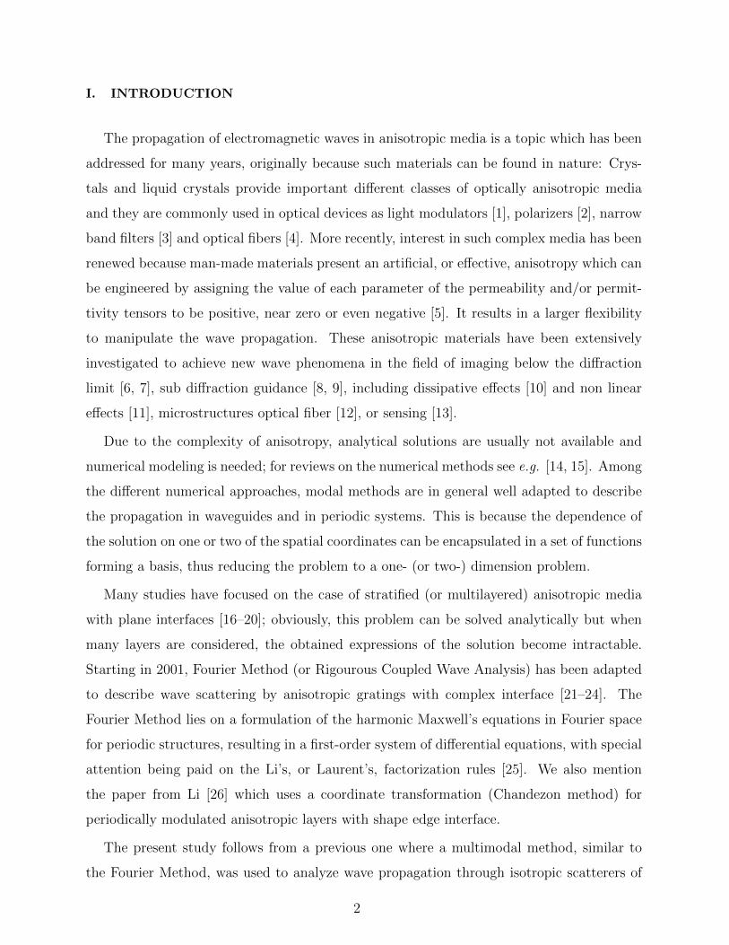
multimodal formulation is presented in the case of periodic media (Figure 1) for TM waves,

the case of TE waves being reduced to isotropic media.

FIG. 1. Typical configuration of the study. An incident wave with wave vector k at incidence

θ propagates through a succession of layers and inclusions being h-periodic along the x-direction.

Each layer or inclusion may be composed of an anisotropic medium with principal directions (X,Y )

tilted through an angle α with respect to the (x, y) frame associated to the periodic structure.

A. Notations

We denote (x, y, z) the reference frame associated to the periodic structure and we con-

sider anisotropic media with the principal axes of anisotropy X and Y being rotated along

the Z = z direction through an angle α. In the reference frame

D = tR(3D)α

εX 0 0

0 εY 0

0 0 εZ

R(3D)α E, with R(3D)

α ≡

cosα sinα 0

− sinα cosα 0

0 0 1

. (1)

In TM polarization, we get H = H(x, y)ez and E = Ex(x, y)ex + Ey(x, y)ey, leading to

∇ ·

tRα

ε−1Y 0

0 ε−1X

Rα∇H

+ k2µH = 0, with Rα ≡

cosα sinα

− sinα cosα

, (2)

and all the parameters α, εX , εY and µ vary in space. Evidently, the result applies for

uniaxial media and εZ = εX or εZ = εY , in which case any rotation in the 3D space can be

4

considered. In the following, we use the notations∇.

ε−1xx ε−1

xy

ε−1xy ε−1

yy

∇H+ k2µ H = 0,

−ikEx = ε−1xy ∂xH + ε−1

yy ∂yH, ikEy = ε−1xx∂xH + ε−1

xy ∂yH,

(3)

with ε−1xx ≡ ε−1

Y cos2 α+ε−1X sin2 α, ε−1

xy ≡ (ε−1Y −ε

−1X ) cosα sinα, ε−1

yy ≡ ε−1Y sin2 α+ε−1

X cos2 α.

(4)

Our notations for the inverses permittivities ε−1ij , in Eqs. (4) are not usual, but they are

more tractable for the following. We report in the appendix A the link with the permittivity

tensor ε, as defined in the relation D = εE.

B. Multimodal formulation

We consider a periodic configuration with h-periodicity along the x-axis (Figure 1). Fol-

lowing [27], the wave equation (3) is written in a variational representation

∑i

∫Ωi

dr

− ε−1

xx ε−1xy

ε−1xy ε−1

yy

∇H · ∇Ht + k2µHHt

+∑i

∫∂Ωi

dS

ε−1xx ε−1

xy

ε−1xy ε−1

yy

∇H · n Ht = 0,

(5)

where Ωi denote the regions with constant (ε−1xx , ε

−1xy , ε

−1yy ) and µ values; for readability,

we avoid to indicate explicitly the index (i) on these values. In the above expression,

Ht(r) is a test function compactly supported (thus vanishing for y → ±∞) and h-periodic

along x; its form will be given below. The last integral vanishes because of the bound-

ary conditions at ∂Ωi, being either the boundary between two different media (continuity of ε−1xx ε−1

xy

ε−1xy ε−1

yy

∇H .n), or the boundary of the domain x = 0 and x = h (and the conditions

of periodicity give[(ε−1xx∂xH + ε−1

xy ∂yH)Ht

](x = h) =

[(ε−1xx∂xH + ε−1

xy ∂yH)Ht

](x = 0)). For

y → ±∞, it vanishes because Ht vanishes. Thus, the boundary conditions have been exactly

taken into account in the weak formulation

∑i

∫Ωi

dr

− ε−1

xx ε−1xy

ε−1xy ε−1

yy

∇H · ∇Ht + k2µHHt

= 0. (6)

We now expand H(x, y) onto a basis of ϕm(x) (with Einstein summation convention)

H(x, y) = Hm(y)ϕm(x), (7)

5

and the ϕm functions are chosen as

ϕm(x) =1√heiγmx, with γm ≡ (κ+ 2mπ/h), (8)

where eiκx denotes the dependence of the waves in the x-direction, imposed by the source

term (the incident wave). We now use the following form of the test function: Ht(r) =

Ht(y)ϕn(x), with arbitrary n-value. Integrating (6) over x, the equation ends with∫

dy Ht(y)F (y) =

0 for any Ht, from which F (y) = 0 is deduced. This leads to

d

dy

[∑i

(ε−1yy AnmH

′m + ε−1

xy BnmHm

)]+∑i

(−ε−1

xy BmnH′m − ε−1

xxCnmHm + k2µAnmHm

)= 0,

(9)

where we have defined the matrices

Anm(y) ≡∫ ai+1(y)

ai(y)

dxϕn(x)ϕm(x),

Bnm(y) ≡∫ ai+1(y)

ai(y)

dxϕn(x)ϕ′m(x),

Cnm(y) ≡∫ ai+1(y)

ai(y)

dxϕ′n(x)ϕ′m(x).

(10)

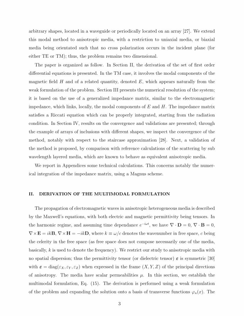
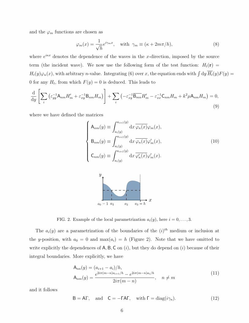
FIG. 2. Example of the local parametrization ai(y), here i = 0, . . . , 3.

The ai(y) are a parametrization of the boundaries of the (i)th medium or inclusion at

the y-position, with a0 = 0 and max(ai) = h (Figure 2). Note that we have omitted to

write explicitly the dependences of A,B,C on (i), but they do depend on (i) because of their

integral boundaries. More explicitly, we have

Ann(y) = (ai+1 − ai)/h,

Anm(y) =e2iπ(m−n)ai+1/h − e2iπ(m−n)ai/h

2iπ(m− n), n 6= m

(11)

and it follows

B = AΓ, and C = −ΓAΓ, with Γ = diag(iγn). (12)

6

Although convolution of the Fourier transformers of two functions have not been used (and

thus, the factorization rules for the Fourier transform of the product of two functions are

not questioned), the projections used in the weak formulation make the Toeplitz matrices

to appear. Indeed, it is easy to see that, for any field g(x, y) (g being for instance the

permeability) ∑i

gA = [g], with [g]nm ≡1

h

∫ h

0

dx g(x, y)e2iπ(m−n)x/h. (13)

Inspecting Eq. (9), it is convenient to re-write the system by introducing an auxiliary field

with modal components Em to get a coupled system of first ordinary differential equations

En ≡ [ε−1yy ]nmH

′m + iγn[ε−1

xy ]nmHm,

E ′n + iγn[ε−1xy ]nmH

′m + (iγn)(iγm)[ε−1

xx ]nmHm + k2[µ]nmHm = 0,(14)

that we express in a matrix form for the two vectors composed by the modal components

E ≡ (Em) and H ≡ (Hm): [ε−1yy ] 0

Γ[ε−1xy ] I

H

E

′ = −[ε−1

xy ]Γ I

−Γ[ε−1xx ]Γ− k2[µ] 0

H

E

, (15)

where all the matrices and the vectors are defined locally at y.

C. Energy conservation

The energy flux across the section at any y-position is defined by

Φ(y) = −1

2Re

[∫dx ExH

]=

1

2kIm[tEH

], (16)

from which ∂yΦ = 1/(2k)Im[tE′H + tEH′

]. The above system (15) can be writtenH

E

′ =M1 M2

M3 M4

H

E

, (17)

with

M1 ≡ −[ε−1yy ]−1[ε−1

xy ]Γ,

M2 ≡ [ε−1yy ]−1,

M3 ≡ Γ([ε−1xy ][ε−1

yy ]−1[ε−1xy ]− [ε−1

xx ])

Γ− k2[µ],

M4 ≡ −Γ[ε−1xy ][ε−1

yy ]−1.

(18)

7

We get

∂yΦ =1

2kIm[tH tM3H + tE M2 E + tE (M4 + tM1) H

]. (19)

In the case where the media are lossless ((ε−1X , ε−1

Y ) and µ are real), the Toeplitz matrices

are self-adjoint and tΓ = −Γ, thus M4 = − tM1 and we get

∂yΦ =1

4k

[tH( tM3 −M3)H + tE(M2 − tM2)E

]. (20)

With M2 and M3 being self-adjoint matrices, the variation of the energy flux vanishes ∂yΦ =

0, which shows that our formulation ensures the energy conservation (see also Ref. [27]).

III. NUMERICAL RESOLUTION

The modal system, Eq. (15), can be solved using several numerical schemes. We use one

scheme of Magnus type, based on an impedance matrix which links the vectors E and H

E = YH. (21)

The matrix Y satisfies a Riccati equation, from Eq. (17),

Y′ = −YM2Y − YM1 − tM1Y + M3. (22)

which is similar to the one obtained in [27] for isotropic media and in [17] for stratified

anisotropic media. To properly integrate the Riccati equation, one has to define the outgoing

and ingoing waves, which is in general quite involved for anisotropic media [31, 32]. As it is

not the subject of the present paper, we consider only real values of the permittivities and

permeabilities, for which no complications occur (Section III A leading to Eq. (25)).This

allows to translate the radiation condition (at y = 0 in Figure 3) as an initial value of the

impedance Yo (section III B), afterwards the system is integrated using a Magnus scheme

toward the entrance of the scattering region (y = `y). This first integration gives the

scattering matrix associated to the scattering region. When needed, the wavefield associated

to a particular source term (incident wave) can be calculated by integrating the same system

from y = `y to y = 0, using the impedance matrices previously computed (Section III C).

The Magnus scheme has been presented elsewhere [27, 33, 34] and we collect in the Appendix

B the principle of the implementation.

8

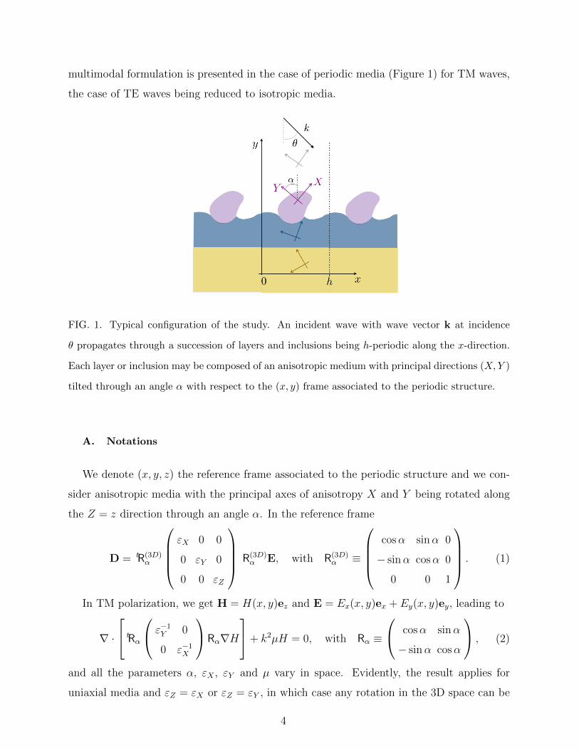
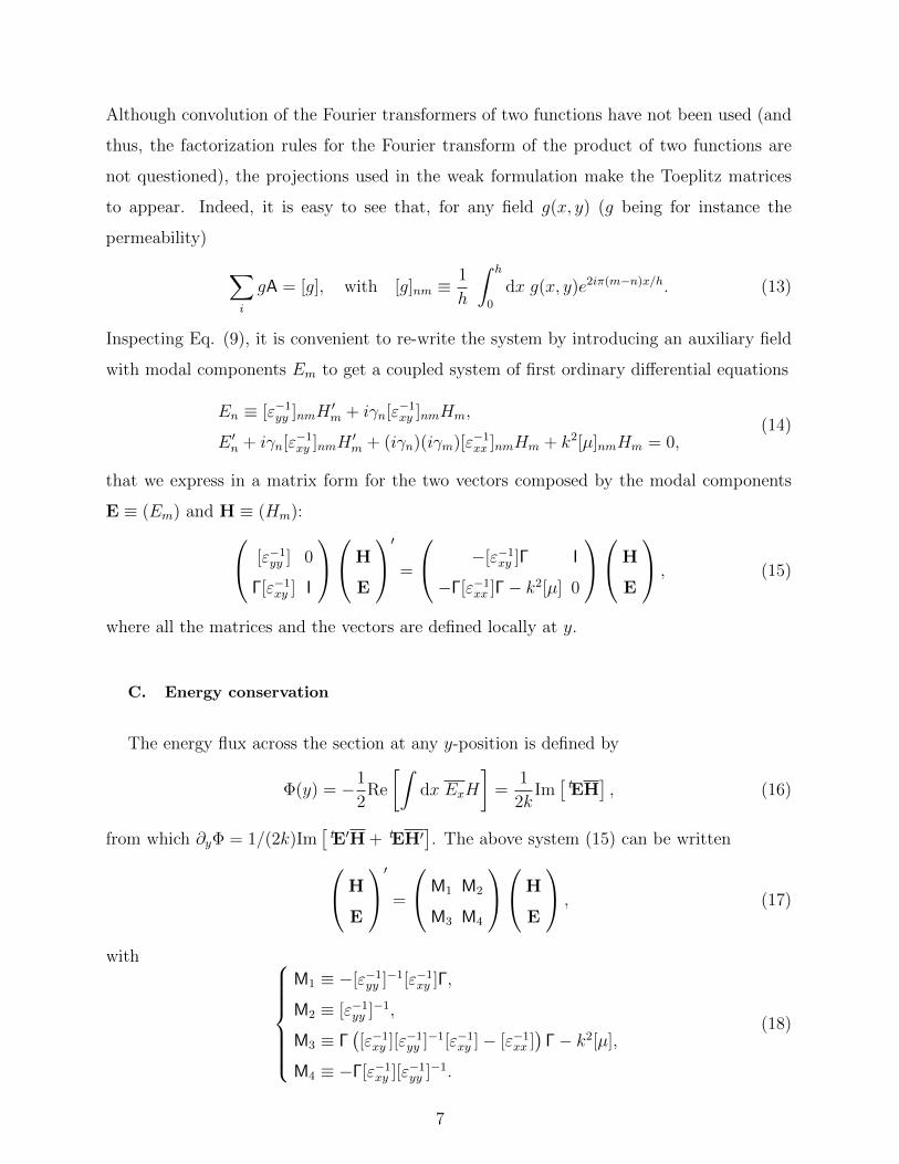
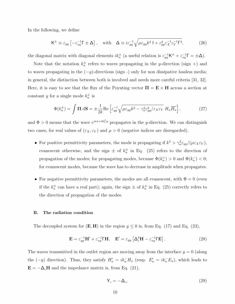
FIG. 3. Regions defined in the numerical scheme: (e) is the entrance medium, y ≥ `y, where the

source is defined (here an incident plane wave) and (o) the outlet region y ≤ 0. Both (o) and

(e) can be anisotropic. In between, the scattering region contains anisotropic inclusions and/or

anisotropic layers, and it corresponds to the domain where the numerical calculations is performed.

A. Mode selection

The two media at the entrance (y ≥ `y) and at the outlet (y ≤ 0) being homogeneous,

we have a0(y) = 0 and a1(y) = h. This implies [g] = gI, and the matrices in Eqs. (17)-(18)

simplify in M1 = M4 = −εyy

εxyΓ,

M2 = εyyI,

M3 =

(εyyε2xy

− 1

εxx

)Γ2 − k2µI = − εyy

εXεYΓ2 − k2µI,

(23)

where we used ε−1yy ε−1xx − ε−2

xy = ε−1X ε−1

Y . The second order equation on the (decoupled) modal

components Hn simplifies in

ε−1yyH

′′n + 2iγnε

−1xyH

′n + (µk2 − γ2

nε−1xx )Hn = 0. (24)

The waves propagating in such medium are of the form eiκx+ikn±y, with the associated

dispersion relation

k±n = −γnεyyεxy±

√µεyyk2 − γ2

n

ε2yy

εXεY. (25)

The link between the above dispersion relation and the usual dispersion relation of birefrin-

gent media (expressed in the frame of the principal directions) is given in the Appendix C.

9

In the following, we define

K± ≡ εyy[−ε−1

xy Γ±∆], with ∆ ≡ iε−1

yy

√µεyyk2 I + ε2

yyε−1X ε−1

Y Γ2, (26)

the diagonal matrix with diagonal elements ik±n (a useful relation is ε−1yy K± + ε−1

xy Γ = ±∆).

Note that the notation k±n refers to waves propagating in the y-direction (sign +) and

to waves propagating in the (−y)-directions (sign -) only for non dissipative lossless media;

in general, the distinction between both is involved and needs more careful criteria [31, 32].

Here, it is easy to see that the flux of the Poynting vector Π = E ×H across a section at

constant y for a single mode k±n is

Φ(k±n ) =

∫Π.dS = ± 1

2kRe[ε−1yy

√µεyyk2 − γ2

nε2yy/εXεY HnHn

], (27)

and Φ > 0 means that the wave eiκx+ik±n y propagates in the y-direction. We can distinguish

two cases, for real values of (εX , εY ) and µ > 0 (negative indices are disregarded).

• For positive permittivity parameters, the mode is propagating if k2 > γ2nεyy/(µεXεY ),

evanescent otherwise, and the sign ± of k±n in Eq. (25) refers to the direction of

propagation of the modes; for propagating modes, because Φ(k+n ) > 0 and Φ(k−n ) < 0;

for evanescent modes, because the wave has to decrease in amplitude when propagates.

• For negative permittivity parameters, the modes are all evanescent, with Φ = 0 (even

if the k±n can have a real part); again, the sign ± of k±n in Eq. (25) correctly refers to

the direction of propagation of the modes.

B. The radiation condition

The decoupled system for (E,H) in the region y ≤ 0 is, from Eq. (17) and Eq. (23),

E = ε−1yy H′ + ε−1

xy ΓH, E′ = εyy[∆2

oH− ε−1xy ΓE

]. (28)

The waves transmitted in the outlet region are moving away from the interface y = 0 (along

the (−y) direction). Thus, they satisfy H ′n = ik−nHn (resp. E ′n = ik−nEn), which leads to

E = −∆oH and the impedance matrix is, from Eq. (21),

Yo = −∆o, (29)

10

where ∆o is defined in Eq. (26), with the characteristics (εxx, εX , εY ) = (εxx, εX , εY )|o and

µ = µo of the medium (o). Alternatively, it is easy to see that Yo is one (constant) solution

of the Riccati equation, Eq. (22), with M3 = −εyy∆2o and

Y′ = −εyy[Y2 −∆2

o

], (30)

and the proper sign is given by the condition of outgoing waves.

Starting from the initial value Y(0) = Yo, the differential system Eq. (22) can be inte-

grated using a Magnus scheme as described in the Appendix B. In the following, we denote

Ye the computed impedance matrix, Y(`y) = Ye.

C. The source term

We consider any source in (e) being a superposition of waves propagating in the (−y)-

direction: H in ∝ eik

−eny+iκx, where the k±en are defined in Eq. (25) with (εxx, εX , εY ) =

(εxx, εX , εY )|e and µ = µe. Then, the reflected field is a superposition of waves propagating

in the +y-direction Hrn ∝ eik

+eny+iκx. The reflection matrix R is defined for the vectors of

modal components Hr = RHi. With K±e being defined in Eq. (26) in (e), we have for the

total field H = Hi + Hr

H′ =(K−e + K+

e R)

Hi. (31)

Using the relation H′ =[εyy(E− ε−1

xy ΓH)]|e, we get (K−e + K+

e R) = εyy (I + R)(Ye + ε−1

xy Γ)

and eventually

R = [∆e − Ye]−1[∆e + Ye]. (32)

In the simplest case where (e) is made of an isotropic material (ε−1yy = ε−1

xx = 1/ε, ε−1xy = 0

and ∆e = −K), we recover R = [K + Ye]−1[K− Ye], as in [27].

D. Validation for a single interface between two anisotropic media

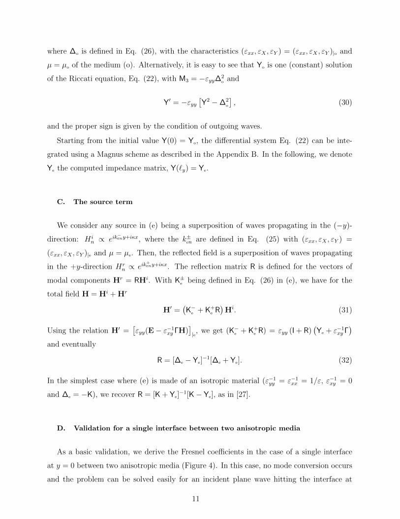
As a basic validation, we derive the Fresnel coefficients in the case of a single interface

at y = 0 between two anisotropic media (Figure 4). In this case, no mode conversion occurs

and the problem can be solved easily for an incident plane wave hitting the interface at

11

incidence θ (κ = k sin θ), leading to H(x, y < 0) = eik sin θx[eik

−e y +Reik

+e y],

H(x, y ≥ 0) = eik sin θx Teik−o y,

(33)

FIG. 4. Single interface between two anisotropic media .

The wavenumber k±e (resp. k±o ) satisfies the dispersion relation ε−1yy (k±)2 + 2ε−1

xy κk± +

(ε−1xxκ

2 − µk2) = 0, leading to

k± = εyyk(−ε−1xy sin θ ± δ), with δ ≡

√µε−1

yy − ε−1X ε−1

Y sin2 θ, (34)

that applies for k±e and for k±e . Obviously, this coincides with the expression of k±n with n = 0

in Eq. (25), since the present problem involves the mode 0 only. Applying the continuity of

H and of ε−1xy ∂xH + ε−1

xx∂yH at the interface y = 0 leads to the expression of the reflection

coefficient R

R =δe − δoδe + δo

. (35)

In [35], the reflection coefficient for an interface between air at y > 0 and an anisotropic

medium with µ = 1 and α = 0 is derived; in that case, our expression simplifies with µe = 1

leading to δe = cos θ and (µo = 1, εyy,o = εX), leading to

R(air, α = 0) =cos θ −

√ε−1X − ε

−1X ε−1

Y sin2 θ

cos θ +√ε−1X − ε

−1X ε−1

Y sin2 θ, (36)

in agreement with the Eq. (7) in Ref [35]. Also, coming back to the general case, we get,

from Eq. (35), a generalization of the Brewster angle, realizing perfect transmission (δe = δo)

θB = asin

√εXεYεyy

εyy − 1

εXεY − 1, (37)

12

which coincides with the result in [35] for α = 0,

Finally, it was our aim to check that this expression is consistent with our numerical

scheme: The Eqs. (34) and (26) show that ∆e,00 = ikδe and ∆o,00 = ikδo. Thus the reflection

coefficient derived for a single interface R coincides with R00, the reflection coefficient of the

mode 0 for an incident wave in mode 0 of the reflection matrix R in Eq. (32), as expected.

IV. CONVERGENCE AND VALIDATION OF THE NUMERICAL METHOD

To validate our numerical method, we consider two different examples:

• First, the convergence of the method is inspected in a problem of scattering by arrays of

anisotropic inclusions. Three different shapes of the inclusions are considered to inspect

the sensitivity of our modal formulation to the problem of staircase approximation

[28]. To anticipate, and as already mentioned in a previous study [27], our formalism

presents the same order of magnitude in the error and the same rate of convergence

for various shapes, being piecewise constant or not, and this tends to prove that the

Li’s rules are not questioned in our formalism.

• We also propose a validation of our method by comparison with direct calculations

of the scattering by a subwavelength layered medium. Beyond the validation of our

formalism, such calculations are of interest. Indeed, one source of interest in the

anisotropic structures is their ability to describe the behavior of subwavelenght layered

media, invoking the theory of homogenization. When applicable, the numerical cost

is obviously much lower since the microstructure has not to be resolved. We inspect

this equivalence between anisotropic media and layered media through the example of

guided waves propagating in a guide made of dielectric slanted layers.

A. Convergence: Scattering by an array of anisotropic inclusions of various shapes

As a first illustrative example, Figures 5 show the real part of the wavefield H(x, y)

resulting from the interaction of an incident plane wave with a h-periodic array of anisotropic

discs of radius R. Calculations have been performed for kR = 3 and kh = 10, and a wave

incident on the array with an angle θ = 45 with the array. The discs are made of an

13

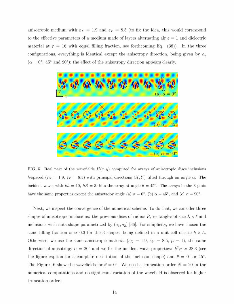
anisotropic medium with εX = 1.9 and εY = 8.5 (to fix the idea, this would correspond

to the effective parameters of a medium made of layers alternating air ε = 1 and dielectric

material at ε = 16 with equal filling fraction, see forthcoming Eq. (38)). In the three

configurations, everything is identical except the anisotropy direction, being given by α,

(α = 0, 45 and 90); the effect of the anisotropy direction appears clearly.

FIG. 5. Real part of the wavefields H(x, y) computed for arrays of anisotropic discs inclusions

h-spaced (εX = 1.9, εY = 8.5) with principal directions (X,Y ) tilted through an angle α. The

incident wave, with kh = 10, kR = 3, hits the array at angle θ = 45. The arrays in the 3 plots

have the same properties except the anisotropy angle (a) α = 0, (b) α = 45, and (c) α = 90.

Next, we inspect the convergence of the numerical scheme. To do that, we consider three

shapes of anisotropic inclusions: the previous discs of radius R, rectangles of size L× ` and

inclusions with nuts shape parametrized by (a1, a2) [36]. For simplicity, we have chosen the

same filling fraction ϕ ' 0.3 for the 3 shapes, being defined in a unit cell of size h × h.

Otherwise, we use the same anisotropic material (εX = 1.9, εY = 8.5, µ = 1), the same

direction of anisotropy α = 20 and we fix the incident wave properties: k2ϕ ' 28.3 (see

the figure caption for a complete description of the inclusion shape) and θ = 0 or 45.

The Figures 6 show the wavefields for θ = 0. We used a truncation order N = 20 in the

numerical computations and no significant variation of the wavefield is observed for higher

truncation orders.

14

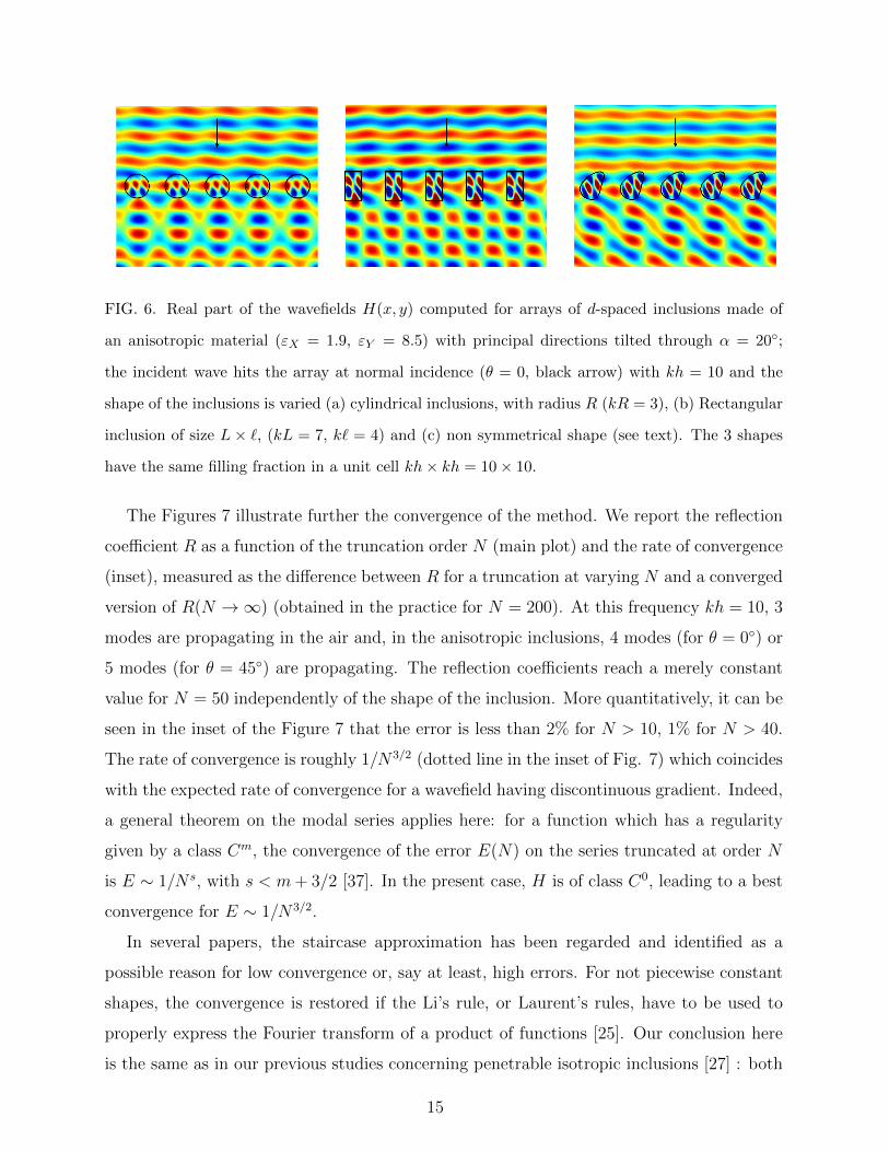
FIG. 6. Real part of the wavefields H(x, y) computed for arrays of d-spaced inclusions made of

an anisotropic material (εX = 1.9, εY = 8.5) with principal directions tilted through α = 20;

the incident wave hits the array at normal incidence (θ = 0, black arrow) with kh = 10 and the

shape of the inclusions is varied (a) cylindrical inclusions, with radius R (kR = 3), (b) Rectangular

inclusion of size L × `, (kL = 7, k` = 4) and (c) non symmetrical shape (see text). The 3 shapes

have the same filling fraction in a unit cell kh× kh = 10× 10.

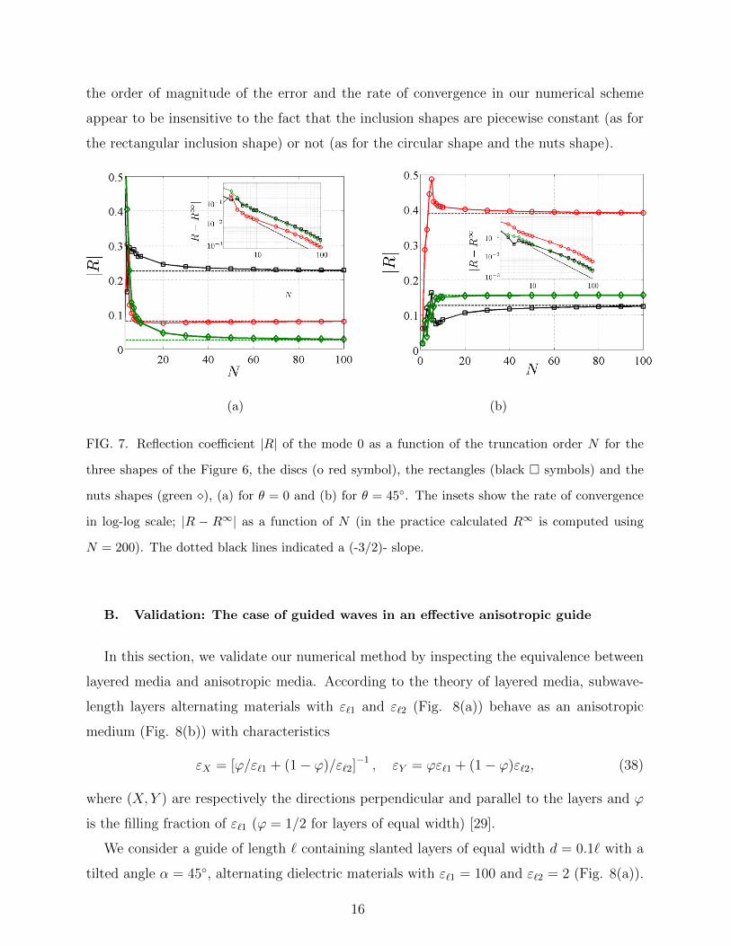
The Figures 7 illustrate further the convergence of the method. We report the reflection

coefficient R as a function of the truncation order N (main plot) and the rate of convergence

(inset), measured as the difference between R for a truncation at varying N and a converged

version of R(N →∞) (obtained in the practice for N = 200). At this frequency kh = 10, 3

modes are propagating in the air and, in the anisotropic inclusions, 4 modes (for θ = 0) or

5 modes (for θ = 45) are propagating. The reflection coefficients reach a merely constant

value for N = 50 independently of the shape of the inclusion. More quantitatively, it can be

seen in the inset of the Figure 7 that the error is less than 2% for N > 10, 1% for N > 40.

The rate of convergence is roughly 1/N3/2 (dotted line in the inset of Fig. 7) which coincides

with the expected rate of convergence for a wavefield having discontinuous gradient. Indeed,

a general theorem on the modal series applies here: for a function which has a regularity

given by a class Cm, the convergence of the error E(N) on the series truncated at order N

is E ∼ 1/N s, with s < m+ 3/2 [37]. In the present case, H is of class C0, leading to a best

convergence for E ∼ 1/N3/2.

In several papers, the staircase approximation has been regarded and identified as a

possible reason for low convergence or, say at least, high errors. For not piecewise constant

shapes, the convergence is restored if the Li’s rule, or Laurent’s rules, have to be used to

properly express the Fourier transform of a product of functions [25]. Our conclusion here

is the same as in our previous studies concerning penetrable isotropic inclusions [27] : both

15

the order of magnitude of the error and the rate of convergence in our numerical scheme

appear to be insensitive to the fact that the inclusion shapes are piecewise constant (as for

the rectangular inclusion shape) or not (as for the circular shape and the nuts shape).

(a) (b)

FIG. 7. Reflection coefficient |R| of the mode 0 as a function of the truncation order N for the

three shapes of the Figure 6, the discs (o red symbol), the rectangles (black symbols) and the

nuts shapes (green ), (a) for θ = 0 and (b) for θ = 45. The insets show the rate of convergence

in log-log scale; |R − R∞| as a function of N (in the practice calculated R∞ is computed using

N = 200). The dotted black lines indicated a (-3/2)- slope.

B. Validation: The case of guided waves in an effective anisotropic guide

In this section, we validate our numerical method by inspecting the equivalence between

layered media and anisotropic media. According to the theory of layered media, subwave-

length layers alternating materials with ε`1 and ε`2 (Fig. 8(a)) behave as an anisotropic

medium (Fig. 8(b)) with characteristics

εX = [ϕ/ε`1 + (1− ϕ)/ε`2]−1 , εY = ϕε`1 + (1− ϕ)ε`2, (38)

where (X, Y ) are respectively the directions perpendicular and parallel to the layers and ϕ

is the filling fraction of ε`1 (ϕ = 1/2 for layers of equal width) [29].

We consider a guide of length ` containing slanted layers of equal width d = 0.1` with a

tilted angle α = 45, alternating dielectric materials with ε`1 = 100 and ε`2 = 2 (Fig. 8(a)).

16

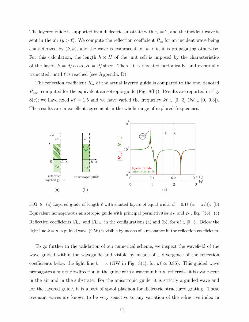
The layered guide is supported by a dielectric substrate with ε2 = 2, and the incident wave is

sent in the air (y > `). We compute the reflection coefficient Rex for an incident wave being

characterized by (k, κ), and the wave is evanescent for κ > k, it is propagating otherwise.

For this calculation, the length h × H of the unit cell is imposed by the characteristics

of the layers h = d/ cosα,H = d/ sinα. Then, it is repeated periodically, and eventually

truncated, until ` is reached (see Appendix D).

The reflection coefficient Rex of the actual layered guide is compared to the one, denoted

Ranis, computed for the equivalent anisotropic guide (Fig. 8(b)). Results are reported in Fig.

8(c); we have fixed κ` = 1.5 and we have varied the frequency k` ∈ [0, 3] (kd ∈ [0, 0.3]).

The results are in excellent agreement in the whole range of explored frequencies.

FIG. 8. (a) Layered guide of length ` with slanted layers of equal width d = 0.1` (α = π/4). (b)

Equivalent homogeneous anisotropic guide with principal permittivities εX and εY , Eq. (38). (c)

Reflection coefficients |Rex| and |Ranis| in the configurations (a) and (b), for k` ∈ [0, 3]. Below the

light line k = κ, a guided wave (GW) is visible by means of a resonance in the reflection coefficients.

To go further in the validation of our numerical scheme, we inspect the wavefield of the

wave guided within the waveguide and visible by means of a divergence of the reflection

coefficients below the light line k = κ (GW in Fig. 8(c), for k` ' 0.85). This guided wave

propagates along the x-direction in the guide with a wavenumber κ, otherwise it is evanescent

in the air and in the substrate. For the anisotropic guide, it is strictly a guided wave and

for the layered guide, it is a sort of spoof plasmon for dielectric structured grating. These

resonant waves are known to be very sensitive to any variation of the refractive index in

17

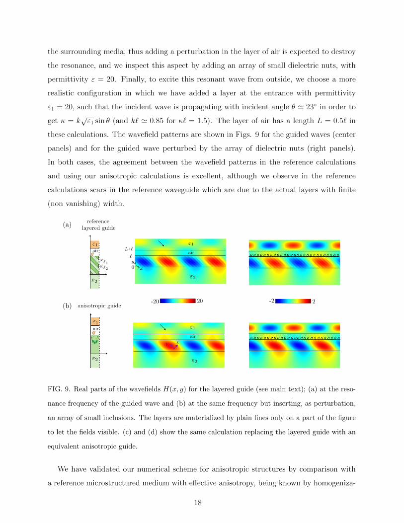
the surrounding media; thus adding a perturbation in the layer of air is expected to destroy

the resonance, and we inspect this aspect by adding an array of small dielectric nuts, with

permittivity ε = 20. Finally, to excite this resonant wave from outside, we choose a more

realistic configuration in which we have added a layer at the entrance with permittivity

ε1 = 20, such that the incident wave is propagating with incident angle θ ' 23 in order to

get κ = k√ε1 sin θ (and k` ' 0.85 for κ` = 1.5). The layer of air has a length L = 0.5` in

these calculations. The wavefield patterns are shown in Figs. 9 for the guided waves (center

panels) and for the guided wave perturbed by the array of dielectric nuts (right panels).

In both cases, the agreement between the wavefield patterns in the reference calculations

and using our anisotropic calculations is excellent, although we observe in the reference

calculations scars in the reference waveguide which are due to the actual layers with finite

(non vanishing) width.

FIG. 9. Real parts of the wavefields H(x, y) for the layered guide (see main text); (a) at the reso-

nance frequency of the guided wave and (b) at the same frequency but inserting, as perturbation,

an array of small inclusions. The layers are materialized by plain lines only on a part of the figure

to let the fields visible. (c) and (d) show the same calculation replacing the layered guide with an

equivalent anisotropic guide.

We have validated our numerical scheme for anisotropic structures by comparison with

a reference microstructured medium with effective anisotropy, being known by homogeniza-

18

tion process. In addition to this validation, the equivalence between structured media and

effective anisotropic media is of interest in term of numerical cost. Indeed, dealing with

microstructured media presents two difficulties:

• First, the microstructure has to be captured, even roughly, which implies a sufficient

truncation order N . Although this is not an heavy constraint in the presented cases

(N ∼ 10), it may become much heavier for more complex interface shapes.

• The length of the unit cell increases with α as h = d/ cosα (Appendix D). This is

penalizing for large α-angle, since it produces an increasing number of propagating

modes that have to be accounted for in the computation.

V. CONCLUSION

We have presented a multimodal method based on the use of the admittance matrix to

describe the propagation of electromagnetic waves in anisotropic periodic media, containing

arbitrary shaped anisotropic inclusions or anisotropic media with arbitrary shaped inter-

faces, or both. Our coupled wave equations are based on a weak formulation, which avoids

to deal with the Fourier transform of a product of functions, and thus, does not address

the Li’s rules. Together with the local admittance formulation, it leads to an efficient and

easily implementable numerical method, well suited to describe continuously variable shape

of scatterers, beyond the usual staircase approximation (the error, as the rate of convergence

have been shown to be independent of the inclusion shape). The method has been shown to

have a good convergence for wave fields presenting discontinuous gradients, namely varying

as N−3/2, N being the truncation order in the modal expansion. A validation of our numer-

ical method has been presented by comparison with microstructured medium presenting an

effective anisotropy at the wave scale.

In the present study, we have considered media with real permittivity and permeability

and no spatial dispersion. These constraints are only motivated by the ease, for such material

properties, in selecting right- and left- going waves which is necessary to properly account

for the radiation condition (Sec. III A). The extension of the presented method to more

complex, and more realistic, material properties is straightforward if the problem of the

selection of these waves is addressed.

19

In general, the modal methods can be applied quasi indifferently to the case of perio-

dic arrays and to the case of waveguides (owing to a change in the modal basis). In the

present case, we see an interesting limitation for the extension of our method to the case

of waveguides with perfectly conducting walls. Indeed, the nice property that the modal

system is decoupled outside the scattering region relies on the choice of the modal basis

ϕm(x): the expansion of H on the ϕm has to satisfy the boundary condition at x = 0, h for

any truncation outside the scattering region. This is needed to properly define the initial

value of the impedance matrix, or in other words, to properly select the modes propagating

away from the scattering region; if not the case, the method fails. The situation is different

if the boundary conditions are not satisfied inside the scattering region; in this case, the

convergence is altered but the modal method still holds. In the present case, the condition

of pseudo-periodicity is satisfied by ϕm(x) and by ϕ′m(x), and this ensures that the expansion

of H satisfies the right boundary condition. In perfectly conducting waveguides, Neumann

boundary conditions apply. For isotropic media, only vanishing first derivatives of the basis

functions are needed, and this is obtained using the usual cosine functions. For anisotropic

media, this would require vanishing values of the functions and the first derivatives. The

problem being identified, it should be possible to find a new basis with such properties and

works are in progress in this direction.

ACKNOWLEDGMENTS

A.M. thanks the support of LABEX WIFI (Laboratory of Excellence within the French

Program Investments for the Future) under references ANR-10-LABX-24 and ANR-10-

IDEX-0001-02 PSL*.

[1] S. Brugioni and R. Meucci, ”Characterization of a nematic liquid crystal light modulator for

mid-infrared applications,” Optics Comm.216, 453-458 (2003).

[2] H. Ren and S.T. Wu, ”Anisotropic liquid crystal gels for switchable polarizers and displays,”

Appl. Phys. Lett. 81(8), 1432-1434 (2002).

[3] C.Y. Chen, C.L. Pan, C.F. Hsieh, Y. F. Lin and R.P. Pan, ”Liquid-crystal-based terahertz

tunable Lyot filter,” Appl. Phys. Lett. 88(10), 101107 (2006).

20

[4] P. K. Choudhury and W. K. Soon, ”On the tapered optical fibers with radially anisotropic

liquid crystal clad,” Progress In Electromagnetics Research 115, 461-475 (2011).

[5] N. Singh, A. Tuniz, R. Lwin, S. Atakaramians, A. Argyros, S.C. Fleming and B.T. Kuhlmey,

”Fiber-drawn double split ring resonators in the terahertz range,” Optic. Mater. Exp. 2(9),

1254-1259 (2012).

[6] J. B. Pendry, ”Negative refraction makes a perfect lens,” Phys. Rev. Lett. 85(18), 3966-3969

(2000).

[7] Z. Jacob, L. V. Alekseyev, and E. Narimanov, ”Optical Hyperlens: Far-field imaging beyond

the diffraction limit,” Opt. Express 14(18), 8247-8256 (2006).

[8] M. Yan N.A. and Mortensen, ”Hollow-core infrared fiber incorporating metal-wire metamate-

rial,” Opt. Express 17(17), 14851-14864 (2009).

[9] S. Atakaramians, A. Argyros, S.C. Fleming and B.T. Kuhlmey, ”Hollow-core waveguides with

uniaxial metamaterial cladding: modal equations and guidance conditions,” J. Opt. Soc. Am.

B 29(9), 2462-2477 (2012).

[10] S. Atakaramians, A. Argyros, S.C. Fleming and B.T. Kuhlmey, ”Hollow-core uniaxial meta-

material clad fibers with dispersive metamaterials,” J. Opt. Soc. Am. B 30(4), 851-867 (2013).

[11] J.Y. Yan, L. Li and J. Xiao, ”Ring-like solitons in plasmonic fiber waveguides composed of

metal-dielectric multilayers,” Opt. Express, 20(3), 1945-1952 (2012).

[12] A. Argyros, ”Microstructures in polymer fibres for optical fibres, THz waveguides, and fibre-

based metamaterials,” ISRN Optics 2013, 785162 (2013).

[13] R. Melik, E. Unal, N. K. Perkgoz, C. Puttlitz, and H. V. Demir, ”Metamaterial-based wireless

strain sensors,” Appl. Phys. Lett. 95(1), 011106 (2009).

[14] P.P Banerjee and J.M. Jarem, ”Computational methods for electromagnetic and optical sys-

tems,” CRC Press. (2000).

[15] E. Popov, ”Gratings: theory and numeric applications,” E. Popov ed., Institut Fresnel (2012).

[16] J. Schesser and G. Eichmann, ”Propagation of plane waves in biaxially anisotropic layered

media,” J. Opt. Soc. Am. 62(6), 786-791 (1972).

[17] J.B. Titchener, and J.R. Willis, ”The reflection of electromagnetic waves from stratified

anisotropic media,” Antennas and Propagation, IEEE Trans. 39(1), 35-39 (1991).

[18] T.M. Grzegorczyk, X. Chen, J. Pacheco, J. Chen, B.I. Wu and J.A. Kong, ”Reflection coeffi-

cients and Goos-Hanchen shifts in anisotropic and bianisotropic left-handed metamaterials,”

21

Prog. In Elect. Res. 51, 83-113 (2005).

[19] E.L. Tan, ”Recursive asymptotic impedance matrix method for electromagnetic waves in bian-

isotropic media,” Microwave and Wireless Components Lett., IEEE 16(6), 351-353 (2006).

[20] K.V. Sreekanth and T. Yu, ”Long range surface plasmons in a symmetric graphene system

with anisotropic dielectrics,” J. Optics, 15(5), 055002 (2013).

[21] E. Popov and M. Neviere, ”Maxwell equations in Fourier space: fast-converging formulation

for diffraction by arbitrary shaped, periodic, anisotropic media,” J. Opt. Soc. Am. A 18

2886-2894 (2001).

[22] K. Watanabe, R. Petit and M. Neviere, ”Differential theory of gratings made of anisotropic

materials,” J. Opt. Soc. Am. A 19(2), 325-334 (2002).

[23] K. Watanabe, J. Pistora, M. Foldyna, K. Postava and J. Vlcek, ”Numerical study on the

spectroscopic ellipsometry of lamellar gratings made of lossless dielectric materials,” J. Opt.

Soc. Am. A 22(4), 745-751 (2005).

[24] T. Magath, ”Coupled integral equations for diffraction by profiled, anisotropic, periodic struc-

tures,” Antennas and Propagation, IEEE Trans. 54(2), 681-686 (2006).

[25] L. Li, ”Use of Fourier series in the analysis of discontinuous periodic structures” J. Opt. Soc.

Am. A 3, 1870-1876 (1996).

[26] L. Li, ”Oblique-coordinate-system-based Chandezon method for modeling one-dimensionally

periodic, multilayer, inhomogeneous, anisotropic gratings,” J. Opt. Soc. Am. A 16(10), 2521-

2531 (1999).

[27] A. Maurel, J.-F. Mercier and S. Felix, ”Wave propagation through penetrable scatterers in a

waveguide and through a penetrable grating,” J. Acoust. Soc. Am. 135(1) 165-174 (2012).

[28] E. Popov, M. Neviere, B. Gralak and G. Tayeb, ”Staircase approximation validity for

arbitrary-shaped gratings,” J. Opt. Soc. Am. A, 19(1), 33-42 (2002).

[29] A. Maurel, S. Felix and J.-F. Mercier, ”Enhanced transmission through gratings: Structural

and geometrical effects,” Phys. Rev. B 88, 115416 (2013).

[30] P.-H. Tsao, ”Derivation and implications of the symmetry property of the permittivity tensor,”

Am. J. Phys. 61(9) 823-825 (1993).

[31] G. Tayeb, ”Contribution a l’etude de la diffraction des ondes electromagnetiques par des

reseaux. Reflexions sur les methodes existantes et sur leur extension aux milieux anisotropes,”

Ph.D. dissertation, No. 90/Aix 3/0065 (University of Aix-Marseille, France, 1990).

22

[32] D. R. Smith and D. Schurig, ”Electromagnetic wave propagation in media with indefinite

permittivity and permeability tensors,” Phys. Rev. Lett. 90(7), 077405 (2003).

[33] V. Pagneux, ”Multimodal admittance method and singularity behaviour at high frequencies,”

J. Comp. App. Maths. 234(6), 1834-1841 (2010).

[34] S. Felix, A. Maurel and J.-F. Mercier, ”Local transformation leading to an efficient Fourier

modal method for perfectly conducting gratings,” J. Opt. Soc. Am. A, 31(10) 2249-2255

(2014).

[35] Y. Huang, B. Zhao, and L. Gao, ”Goos-Hanchen shift of the reflected wave through an

anisotropic metamaterial containing metal/dielectric nanocomposites,” J. Opt. Soc. Am. A

29(7), 1436-1444 (2012).

[36] The parametrization of the nuts shape is given by, (i) with y1/h = 0.175 cos t+2.5, a1(y1)/h =

0.15(y1) + (y1 − 5)2/2 + 0.125 sin t − 0.4 and (ii) with y2/h = 0.175 cos t + 2.5, a2(y2)/h =

0.3y2/H + 2(y2/H − 2.5)2 + 0.125 sin t− 0.4.

[37] C. Hazard, and E. Luneville, ”An improved multimodal approach for non uniform acoustic

waveguide,” IMA J. Appl. Math. 73 668-690 (2008).

[38] K. Watanabe, ”Numerical integration schemes used on the differential theory for anisotropic

gratings,” J. Opt. Soc. Am. A 19(11), 2245-2252 (2002).

Appendix A: The permittivity tensor

In our formulation, Eq. (1), D = εE with ε expressed in the frame (x, y)

ε =

ε11 = εX cos2 α + εY sin2 α ε12 = (εX − εY ) cosα sinα 0

ε12 ε22 = εX sin2 α + εY cos2 α 0

0 0 εZ

. (A1)

For TM waves, E and D are in plane vectors (Ez = Dz = 0) associated to the permittivity

tensor in 2D

ε ≡

ε11 ε12

ε12 ε22

. (A2)

and our notations for ε−1IJ (I, J are x or y) in Eqs. (4) are linked to the usual εij (i, j are 1

23

or 2) in the permittivity tensor by ε−1xx ε−1

xy

ε−1xy ε−1

yy

=1

det(ε)ε, (A3)

with det(ε) = εXεY (or ε−1IJ = εij/(εXεY )). Eq. (2) reads

∇ ·[

1

det(ε)ε∇H

]+ k2µH = 0. (A4)

Appendix B: Integration of the Riccati equation; Magnus scheme

The integration of the modal system, Eq. (17) needs care. First, the contamination by

exponentially growing evanescent modes has to be avoided. Second, the original problem

is posed as a boundary value problem, with a forcing source at y = `y and a radiation

condition at y = 0. Therefore, the coupled first-order Eq. (17) cannot be solved directly

as an initial value problem. To circumvent these problems, we implement a multimodal

admittance method which leads to a stable initial value problem.

1. Computation of the scattering matrices

Starting from an initial condition Y(0) = Yo, the admittance matrix is calculated, follow-

ing the scheme Eq. (17) written as a system

F(y)′ = M(y)F(y), with F ≡

H

E

, M =

M1 M2

M3 M4

.

This evolution equation can be solved using a Magnus scheme. With a given discretization

along y with step δy, the solution at y+ δy is given from the solution at y using the matrix

exponential N ≡ eM(y+δy/2)δy defined at the middle position between both; then

F(y + δy) = NF(y), and we denote N ≡

N1 N2

N3 N4

. (B1)

F(0) is unknown, but Y(0) is known and the above equation can be used to find Y(y)

Y(y + dy) = [N3 + N4Y(y)] [N1 + N2Y(y)]−1 , Y(0) = Yo, (B2)

24

which is used from y = 0 (Yo is known from the radiation condition) to y = `y. Together

with the computation of Y, one computes the propagator G defined as

H(0) = G(0, y)H(y), which satisfies G(0, y + δy)H(y + δy) = G(0, y)H(y) with G(0, 0) = I.

This allows to compute G together with Y

G(0, y + δy) = G(0, y) [N1 + YN2]−1 , G(0, 0) = I. (B3)

(incidentally, note that G satisfies also a Riccati equation G′ = −G [M1 + M2Y]).

The calculation of Y and G allows to get the scattering properties of the region (x, y) ∈

[0, h]× [0, `y] in terms of the reflection matrix R and transmission matrix T R = [∆e − Y(`y)]−1 [∆e + Y(`y)] , with H(`y) = [I + R] Hi,

T = G(0, `y) [I + R] , with H(0) = THi,(B4)

for any incident wave Hi. Note that the computations of R and T do not require any storage

of Y and G along the y-axis.

2. Computation of the wavefield for a given source term

If the wavefield resulting from a given source term Hi is regarded, it is sufficient to store

the Y(y) values in the first integration (from y = 0 to y = `y), afterwards the forward

integration (along −y) can be done. In this case, H(`y) = [I + R] Hi being known, we use the

formulation on F in Eq. (B1) to get

H(y) = [N1 + N2Y(y)]−1 H(y + δy). (B5)

3. Remark on the discretization δy along the the y axis

Because the exponential matrix involves real and imaginary terms of the matrix M, δy

has to be chosen to ensure non diverging terms. This is usually done by imposing δy equal

to the inverse of the wavenumber associated to the most evanescent mode. This is consistent

with the physical argument that the spatial discretization has to resolve the smallest scale

associated to the spatial variations in the wavefield. As a rough estimate, the evanescent

25

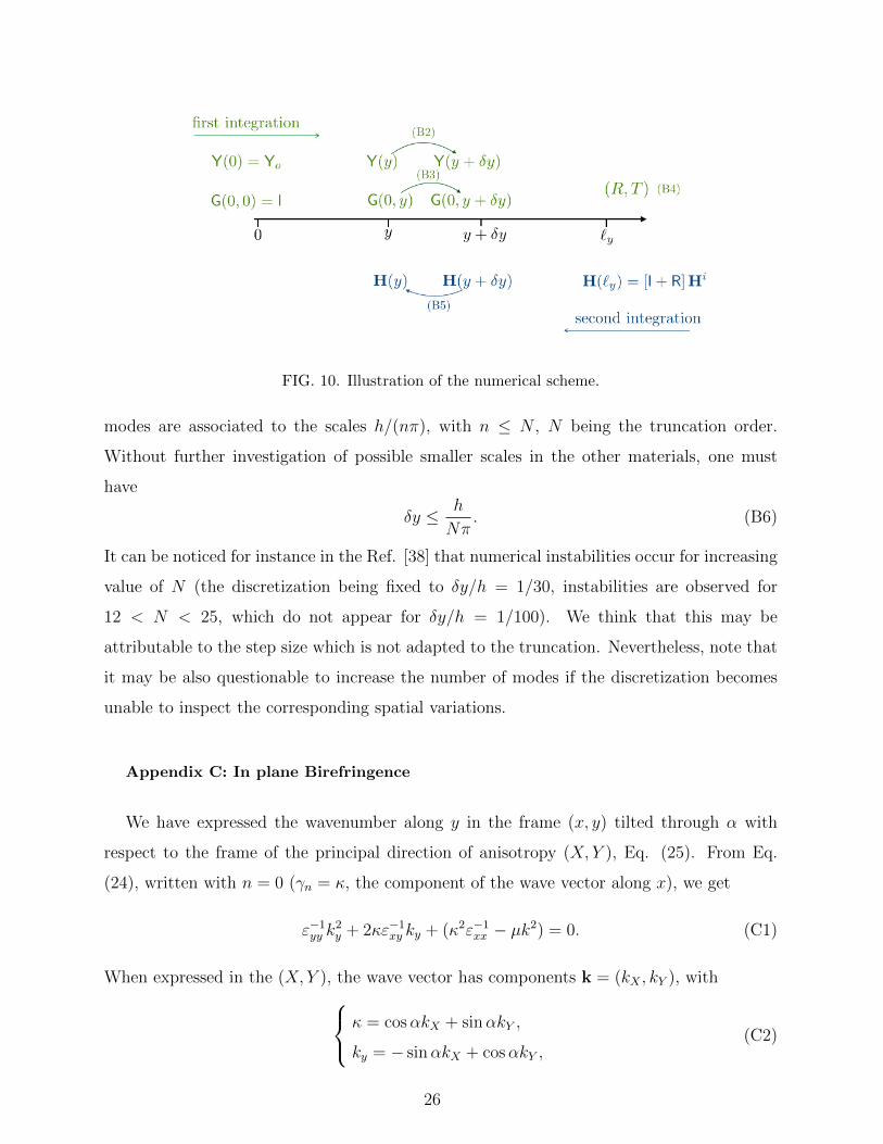
FIG. 10. Illustration of the numerical scheme.

modes are associated to the scales h/(nπ), with n ≤ N , N being the truncation order.

Without further investigation of possible smaller scales in the other materials, one must

have

δy ≤ h

Nπ. (B6)

It can be noticed for instance in the Ref. [38] that numerical instabilities occur for increasing

value of N (the discretization being fixed to δy/h = 1/30, instabilities are observed for

12 < N < 25, which do not appear for δy/h = 1/100). We think that this may be

attributable to the step size which is not adapted to the truncation. Nevertheless, note that

it may be also questionable to increase the number of modes if the discretization becomes

unable to inspect the corresponding spatial variations.

Appendix C: In plane Birefringence

We have expressed the wavenumber along y in the frame (x, y) tilted through α with

respect to the frame of the principal direction of anisotropy (X, Y ), Eq. (25). From Eq.

(24), written with n = 0 (γn = κ, the component of the wave vector along x), we get

ε−1yy k

2y + 2κε−1

xy ky + (κ2ε−1xx − µk2) = 0. (C1)

When expressed in the (X, Y ), the wave vector has components k = (kX , kY ), with κ = cosαkX + sinαkY ,

ky = − sinαkX + cosαkY ,(C2)

26

from which we deduce, using Eqs. (4), the dispersion relation expressed in terms of (kX , kY )

εXk2X + εY k

2Y = µεXεY k

2. (C3)

This is the usual form of the dispersion relation for birefringent medium (if for instance

εZ = εX), restricted here to in plane incidences, which defines the surface of the indices.

Appendix D: Parametrization of layered media

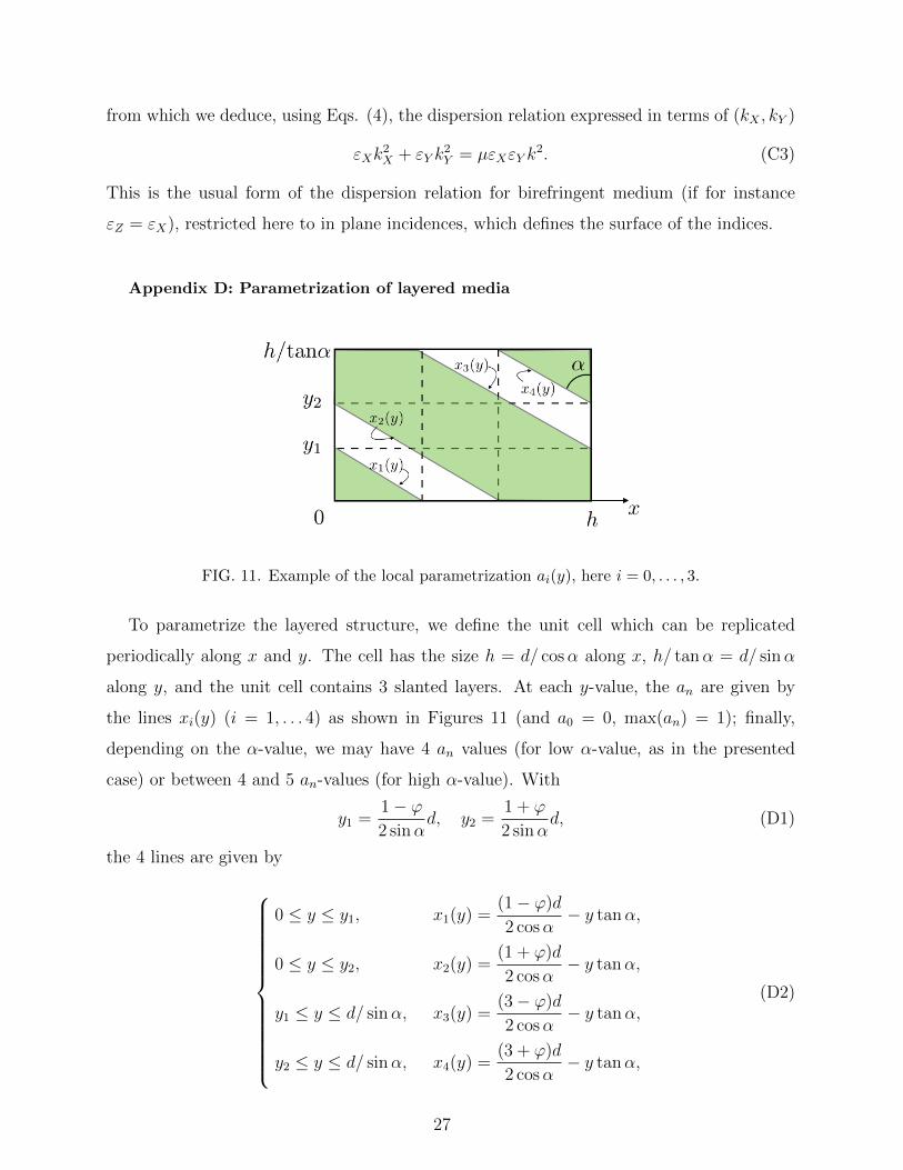
FIG. 11. Example of the local parametrization ai(y), here i = 0, . . . , 3.

To parametrize the layered structure, we define the unit cell which can be replicated

periodically along x and y. The cell has the size h = d/ cosα along x, h/ tanα = d/ sinα

along y, and the unit cell contains 3 slanted layers. At each y-value, the an are given by

the lines xi(y) (i = 1, . . . 4) as shown in Figures 11 (and a0 = 0, max(an) = 1); finally,

depending on the α-value, we may have 4 an values (for low α-value, as in the presented

case) or between 4 and 5 an-values (for high α-value). With

y1 =1− ϕ2 sinα

d, y2 =1 + ϕ

2 sinαd, (D1)

the 4 lines are given by

0 ≤ y ≤ y1, x1(y) =(1− ϕ)d

2 cosα− y tanα,

0 ≤ y ≤ y2, x2(y) =(1 + ϕ)d

2 cosα− y tanα,

y1 ≤ y ≤ d/ sinα, x3(y) =(3− ϕ)d

2 cosα− y tanα,

y2 ≤ y ≤ d/ sinα, x4(y) =(3 + ϕ)d

2 cosα− y tanα,

(D2)

27

Then, the cell can be repeated by shifting the unit cell along y, y = 0→ y = d/ sinα.

28