Chapter 19

ELECTROMAGNETIC WAVE PROPAGATIONIN THE LOWER ATMOSPHERE

Section 19.1 V. J. Falcone, Jr.Section 19.2 R. Dyer

19.1 REFRACTION IN THE 19.1.1 Optical WavelengthsLOWER TROPOSPHERE

An approximate relation between the optical refractiveThe speed of propagation of an electromagnetic wave modulus and atmospheric pressure and temperature is

in free space is a constant, c, which is equal to 3 x 108m/s. In a material medium such as the atmosphere, the speed Pof propagation varies. Even small variations in speed pro- Nx = 77.6 P/T (19.3)duce marked changes in the direction of propagation, thatis, refraction. where Nx is the refractive modulus for wavelengths >20

In the atmosphere, the speed of propagation varies with um, P is atmospheric pressure in millibars, and T is at-changes in composition, temperature, and pressure. At radio mospheric temperature in degrees kelvin.wavelengths, speed does not vary significantly with the The dispersion formula of Edlen [1953],whichhasbeenwavelength, but in the optical region the speed depends adopted by the Joint Commission for Spectroscopy, isstrongly on the wavelength. In the lower 15 km of theatmosphere, water vapor is the most highly variable of the 29498.10 255.40atmospheric gases, and at radio wavelengths the speed of Ns = 64.328 +propagation is strongly affected by water vapor. Temper- 146 - 1/x2 41 - 1/x2ature and pressure variations are principally functions ofaltitude, although for propagation at small elevation angles where Ns is the refractive modulus at a wavelength A for asignificant variations may occur along horizontal distances. temperature of 288 K and a pressure of 1013.25 mb, andFrom the standpoint of effect on the speed of propagation, A is the wavelength in micrometers. A somewhat less precisetemperature variations at any given altitude are more sig- but more convenient dispersion formula isnificant than pressure variations.

In its most general form, the refractive index is a com- .52 x 10-3plex function. The real term of the complex function is N = Nx + x2 (19. 5)called the phase refractive index, n;

Equations (19.3) and (19.5) can be combined to givec

n = - (19.1) the refractive modulus as a function of pressure, tempera-v ture, and wavelength;

where c is the speed of light in a vacuum and v, the phase 77.6 P 0.584 Pvelocity, is the speed of propagation in a particular medium. N T T A2 (19.6)In the troposphere where n is nearly equal to one, it isconvenient to define the quantity Refractive moduli calculated by using Equation (19.6)

will be in error no more than one N-unit over the temperatureN = (n 1) x 106. (19.2) range 243 to 303 K for wavelengths from 0.2 to 20 um.

Thus Equation (19.6) covers the spectrum from the far ul-N is called the refractive modulus; units of (n - 1) x 106 traviolet through the near infrared. A more accurate rela-are called N-units. tionship is given in Chapter 18.

19-1

CHAPTER 19

19.1.2 Radio Wavelengths

At radio wavelengths the relationship of refractive mod- 74494ulus to pressure, temperature, and water-vapor pressure is 261200

given by 600

77.6P 373000PwvN= + (19.7) 700

where Pwv is the partial pressure of water vapor in millibars, 800P is pressure in millibars, and T is temperature in degreeskelvin. Equation (19.7) is accurate to 0.1 N-unit from the 900 M

longest radio wavelengths in use down to about 6 mm (50GHz); 5 N-units from 6 to 4 mm (50 to 75 GHz); and 1 N- 1000

unit from 4 to 2.6 mm (75 to 115 GHz). A more accurate 213 233 253 273 293 303description of refraction and its effects in the 30 to 1000 T (K)

GHz region (EHF range) has been investigated by Liebe[1980]. Figure 19-1. Data from Chatham, Mass. radiosonde release of 26 July

Absorption by atmospheric constituents begins to rise 1982.to significant proportions with decreasing wavelength be-ginning near 1.5 cm. Water vapor content is by far theleading factor in causing changes in N, followed in order 19.1.3 Standard Profiles ofof importance by temperature and pressure. For example, Refractive Modulusfor a temperature of 288 K, pressure of 1013 mb near groundlevel, and a relative humidity of 60% (Pwv = 10 mb), the The vertical distribution of the refractive modulus canfluctuation, AN, is be calculated from Equation (19.3) using vertical distribu-

tions of vapor pressure and temperature as a function ofAN = 4.5 APwv - 1.26 AT + 0.27 AP. (19.8) pressure. Under normal conditions, N tends to decrease

exponentially with height. An exponential decrease is usu-As Equation (19.8) shows, a fluctuation in water vapor ally an accurate description for heights greater than 3 km;pressure has 16 times the effect on the refractive index as below 3 km, N may depart considerably from exponentialthe same amount of fluctuation in total pressure and 3.5 behavior. The median value for the gradient dN is typicallytimes the effect as the same fluctuation in temperature. -0.0394N/m for the first few thousand meters above groundEquation (19.7) may also be used in the windows of relative level.transparency for submillimeter waves (X > 100 um, For many purposes it is desirable to have standard re-f < 3 x 106GHz) with an error of 10 to 20 N-units. fractive-moddulus profiles for the atmosphere. By using the

Equation (19.7) is a function of temperature, pressure, equations of the model atmosphere, an exact analyticaland vapor pressure all of which are height dependent, that expression for the standard optical refractive modulus canis, elevation (h) above the surface; thus N(h) is the refrac- be derived. A simplified approximation to this istivity structure. In reality, surfaces of constant refractivityare not planes, but are concentric spheres about the earth's zcenter. In characterizing the atmospheric layers that affect Nx = 273 exp ( (Z <= 7.62) (19.11)radio wave propagation a modified refractivity structure M(h)

is defined. Z is the altitude in thousands of km.

h Equation (19.11) can be differentiated to obtain theM = (n + - - 1) x 106 (19.9) standard gradient of optical refractive modulus;

a

dN ZM(h) = N(h) + 157h in units of M (19.10) 27.8 exp (Z <= 7.62). (19.12)dZ

where h is in kilometers, a is the radius of the earth (6370km) and 1/a = 157 x 10-6 km-1. Equations (19.11) and (19.12) may be corrected for

When the lapse rate of N is less than - 157 N-units per dispersion through use of Equation (19.5).kilometer [Equation (19.10)], the slope of M becomes neg- For the radio wavelengths, it is necessary to assume aative indicating a ducting condition. Figure 19-1 illustrates distribution of water vapor in order to obtain an expressionducts at 1000 and 700 mb [Morrissey, personal communi- for the refractive modulus. Assuming Pwv = 10.2cation, 1982]. (1 - 0.064Z), for Z < 7.62, a simplified approximation is

19-2

ELECTROMAGNETIC WAVE PROPAGATION IN THE LOWER ATMOSPHERE

7.5 7.5

LAS VEGAS

RADIO (Icm<=X<=500m) 6.0 16 AUGUST 1949

4,5 STANDARD

OPTICAL

1.5

0

100 140 180 220 260 300 340 380-2 -4 -6 -8 -10 -12 MODULUS (N units)

GRADIENT (Nunits per 103 tt)

Figure 19-4. Microwave refractive modulus profile in continental tropicalFigure 19-2. Variation of standard gradient of refractive modulus with air mass.altitude.

19.1.4 Variations of Refractive ModuliN = 316 exp ((Z < 7.62). (19.13)

Actual profiles may differ markedly from the standardThe standard gradient of radio-wave refractive modulus is profiles. Figures 19-4 through 19-7 show some profiles ofthen: refractive modulus at microwave frequencies calculated from

radiosonde measurements. These are considered typical fordNZ=-39.1 exp ( ), (Z 7.62). (19.14) the air masses indicated. Average deviations from a modeldZ 8.08 atmosphere refractive index have been studied extensively;

Figures 19-2 and 19-3 are graphs of standard profiles cal- for example, see Bean and Dutton [1968].culated from Equations (19.12) through (19.14).

7.5

7.5 FAIRBANKS2 JANUARY 1949

6.0

6.0

STANDARD

4.5

1.5

0 100 140 180 220 260 300 340200 300 MODULUS (Nunits)

MODULUS (Nunits)

Figure 19-5. Microwave refractive modulus profile in continental polarFigure 19-3. Variation of standard refractive modulus with altitude. air mass.

19-3

CHAPTER 19

7.5 7.5

SWAN ISLAND30 JULY 1949 6.0 TATOOSH

16 JANUARY1949

4.5

1.5

100 140 180 220 260 300 340 380 100 140 180 220 260 300 340 380

MODULUS (Nunits) MODULUS (Nunits)

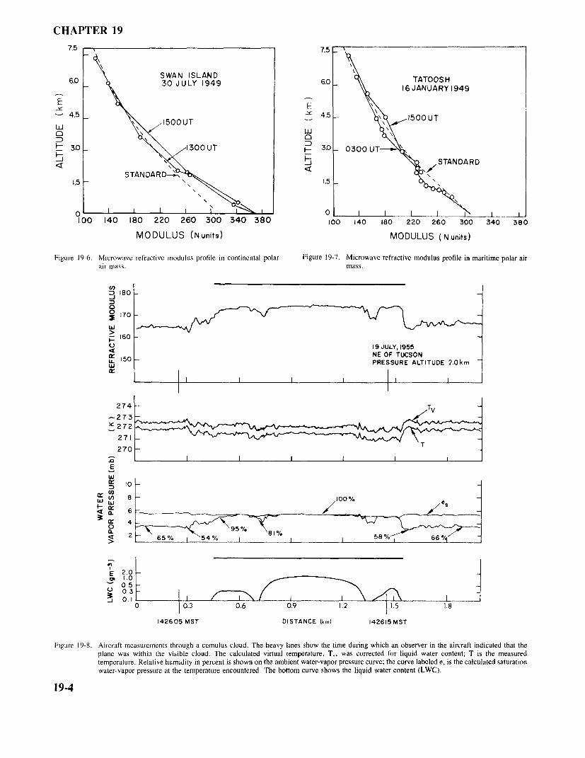
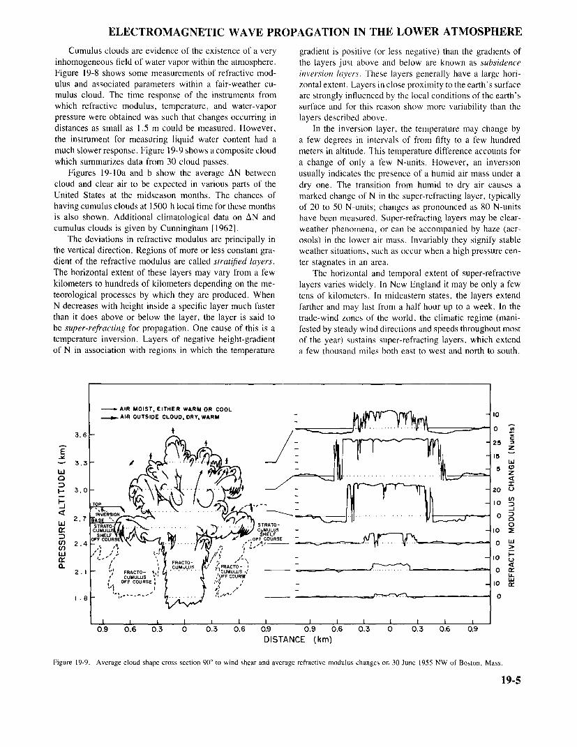
Figure 19-6. Microwave refractive modulus profile in continental polar Figure 19-7. Microwave refractive modulus profile in maritime polar airair mass. mass.

170

19 JULY, 1955NE OF TUCSONPRESSURE ALTITUDE 2.0km

274

270

5

142605 MST DISTANCE (km) 142615 MST

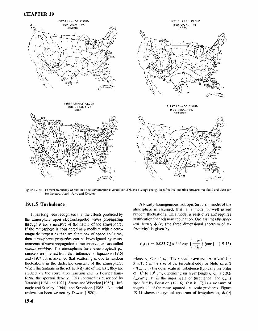
Figure 19-8. Aircraft measurements through a cumulus cloud. The heavy lines show the time during which an observer in the aircraft indicated that theplane was within the visible cloud. The calculated virtual temperature, Tv, was corrected for liquid water content; T is the measuredtemperature. Relative humidity in percent is shown on the ambient water-vapor pressure curve; the curve labeled es is the calculated saturationwater-vapor pressure at the temperature encountered. The bottom curve shows the liquid water content (LWC).

19-4

ELECTROMAGNETIC WAVE PROPAGATION IN THE LOWER ATMOSPHERE

Cumulus clouds are evidence of the existence of a very gradient is positive (or less negative) than the gradients ofinhomogeneous field of water vapor within the atmosphere. the layers just above and below are known as subsidenceFigure 19-8 shows some measurements of refractive mod- inversion layers. These layers generally have a large hori-ulus and associated parameters within a fair-weather cu- zontal extent. Layers in close proximity to the earth's surfacemulus cloud. The time response of the instruments from are strongly influenced by the local conditions of the earth'swhich refractive modulus, temperature, and water-vapor surface and for this reason show more variability than thepressure were obtained was such that changes occurring in layers described above.distances as small as 1.5 m could be measured. However, In the inversion layer, the temperature may change bythe instrument for measuring liquid water content had a a few degrees in intervals of from fifty to a few hundredmuch slower response. Figure 19-9 shows a composite cloud meters in altitude. This temperature difference accounts forwhich summarizes data from 30 cloud passes. a change of only a few N-units. However, an inversion

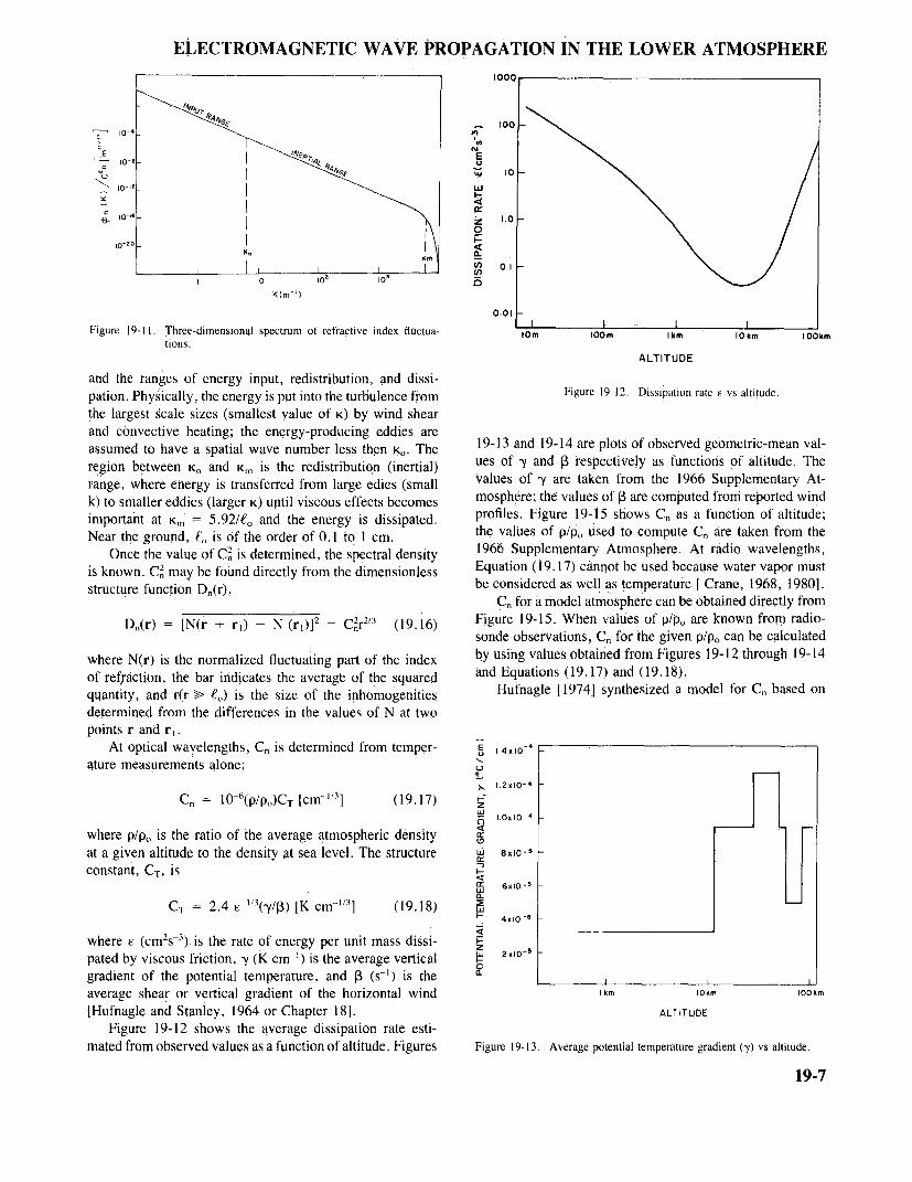
Figures 19-10a and b show the average AN between usually indicates the presence of a humid air mass under acloud and clear air to be expected in various parts of the dry one. The transition from humid to dry air causes aUnited States at the midseason months. The chances of marked change of N in the super-refracting layer, typicallyhaving cumulus clouds at 1500 h local time for these months of 20 to 50 N-units; changes as pronounced as 80 N-unitsis also shown. Additional climatological data on AN and have been measured. Super-refracting layers may be clear-cumulus clouds is given by Cunningham [1962]. weather phenomena, or can be accompanied by haze (aer-

The deviations in refractive modulus are principally in osols) in the lower air mass. Invariably they signify stablethe vertical direction. Regions of more or less constant gra- weather situations, such as occur when a high pressure cen-dient of the refractive modulus are called stratified layers. ter stagnates in an area.The horizontal extent of these layers may vary from a few The horizontal and temporal extent of super-refractivekilometers to hundreds of kilometers depending on the me- layers varies widely. In New England it may be only a fewteorological processes by which they are produced. When tens of kilometers. In mideastern states, the layers extendN decreases with height inside a specific layer much faster farther and may last from a half hour up to a week. In thethan it does above or below the layer, the layer is said to trade-wind zones of the world, the climatic regime (mani-be super-refracting for propagation. One cause of this is a fested by steady wind directions and speeds throughout mosttemperature inversion. Layers of negative height-gradient of the year) sustains super-refracting layers, which extendof N in association with regions in which the temperature a few thousand miles both east to west and north to south.

AIR MOIST, EITHER WARM OR COOLAIR OUTSIDE CLOUD, DRY, WARM

3.6

25

STRATO-O

0.9 0.6 0.3 0 0.3 0.6 0.9 0.9 0.6 0.3 0 0.3 0.6 0.9DISTANCE (km)

Figure 19-9. Average cloud shape cross section 90° to wind shear and average refractive modulus changes on 30 June 1955 NW of Boston, Mass.

19-5

CHAPTER 19FIRST 1.2 km OF CLOUD FIRST 1.2km OF CLOUD

1500 LOCAL TIME 1500 LOCAL TIMEAPRILJANUARY

FIRST 1.2 km OF CLOUD

1500 LOCAL TIME FIRST 1.2km OF CLOUDJULY 1500 LOCAL TIME

OCTOBER

Figure 19-10. Percent frequency of cumulus and cumulonimbus cloud and AN, the average change in refractive modulus between the cloud and clear airfor January, April, July, and October.

19.1.5 Turbulence A locally-homogeneous isotropic turbulent model of theatmosphere is assumed, that is, a model of well mixed

It has long been recognized that the effects produced by random fluctuations. This model is restrictive and requiresthe atmosphere upon electromagnetic waves propagating justification for each new application. One assumes the spec-through it are a measure of the nature of the atmosphere. tral density Xn(K) (the three dimensional spectrum of re-

If the atmosphere is considered as a medium with electro- fractivity) is given bymagnetic properties that are functions of space and time,FIRST 1.2 kmOF CLOUD1500 LOCAL TIME FIRST 1.21km OF CLOUD

JULY 1500 LOCAL TIMEOCTOBER

0%

then atmospheric properties can be investigated by meas-urements of wave propagation; these observations are called Xn4(k) = 0.033 C2n K- 1 1 /3 exp ( [cm3 ] (19.15)remote probing. The atmospheric (or meteorological) pa-rameters are inferred from their influence on Equations (19.6)and (19.7); it is assumed that scattering is due to random where K0 < K < Km The spatial wave number K(cm-1) is

fluctuations in the dielectric constant of the atmosphere. 2 r/l, l is the size of the turbulent eddy or blob, K0 is 2When fluctuations in the refractivity are of interest, they are 2 r/t , l is the outer scale of turbulence (typically the orderstudied via the correlation function and its Fourier trans- of 103 to 104 cm, depending on layer height), Km is 5.92/form, the spectral density. This approach is described by l0(cm-1), lo is the inner scale or turbulence, and C isTatarski [1961 and 1971], Staras and Wheelon [1959], Huf- specified by Equation (19.16), that is, C2n is a measure ofnagle and Stanley [1964]Strohbehn [1968]. A tutorial magnitude of that mean squared fine scale gradients. Figure

review has been written by Dewan [1980]. 19-11 shows the typical spectrum of irregularities, (Xn(K)

19-6

ELECTROMAGNETIC WAVE PROPAGATION IN THE LOWER ATMOSPHERE

1001

IFigure 19-11. Three-dimensional spectrum of refractive index fluctua-

tions,ALTITUDE

and the ranges of energy input, redistribution, and dissi-pation. Physically, the energy is put into the turbulence from Figure 19-12. Dissipation rate vs altitude.

the largest scale sizes (smallest value of K) by wind shearand convective heating; the energy-producing eddies areassumed to have a spatial wave number less then Ko. The 19-13 and 19-14 are plots of observed geometric-mean val-region between Ko and Km is the redistribution (inertial) ues of y and B respectively as functios of altitude. The

values of y are taken from the 1966 Supplementary At-range, where energy is transferred from large edies (smallk) to smaller eddies (larger K) until viscous effects becomes mosphere; the values of B are computed from reported windimportant at Km = 5.92/lo and the energy is dissipated. profiles. Figure 19-15 shows Cn as a function of altitude;Near the ground, lo is of the order of 0. 1 to 1 cm. the values of p/pO used to compute Cn are taken from the

Once the value of C2 is determined, the spectral density 1966 Supplementary Atmosphere. At radio wavelengths,Once the value of C2n is determined, the spectral densityis known. C2n may be found directly from the dimensionless Equation (19.17) cannot be used because water vapor must

be considered as well as temperature [ Crane, 1968, 1980].structure function Dn(r),Cn for a model atmosphere can be obtained directly from

D2(r) = [N(r + r,) - N (r)] 2= Cr 2 3 (19.6) Figure 19-15. When values of p/po are known from radio-D,(r) =[N(r +rl) -N (rl)] 2 r'(1.6

sonde observations, Cn, for the given p/po can be calculated

where N(r) is the normalized fluctuating part of the index by using values obtained from Figures 19-12 through 19-14of refraction, the bar indicates the average of the squared and Equations (19.17) and (19.18).

Hufnagle [1974] synthesized a model for Cn based onquantity, and r(r > lo) is the size of the inhomogenitiesdetermined from the differences in the values of N at twopoints r and r1.

At optical wavelengths, Cn is determined from temper-ature measurements alone;

Cn, 10-6(p/po)CT [cm- 1/3] (19.17)

where p/po is the ratio of the average atmospheric densityat a given altitude to the density at sea level. The structureconstant, CT, is

CT = 2.4 e 1/3(y/B) [K cm - 1/3 ] (19.18)4xlO

where e (cm2 s-3 ) is the rate of energy per unit mass dissi-pated by viscous friction, y (K cm-1) is the average verticalgradient of the potential temperature, and B (s-1) is theaverage shear or vertical gradient of the horizontal wind 1km 10km 1OOkm

[Hufnagle and Stanley, 1964 or Chapter 18]. ALTITUDE

Figure 19-12 shows the average dissipation rate esti-mated from observed values as a function of altitude. Figures Figure 19-13. Average potential temperature gradient (y) vs altitude.

19-7

CHAPTER 19

010 where h is height in meters above sea level, r is a zero meanhomogeneous Gaussian random variable with a covariancefunction given by

(r(h + h', t + T) r(h,t))A(h'/100)e-t/ 5 + A(h'/2000)e-r/ 80 (19.21)

.005

The model for Cn(h, t) is valid for heights between 3 and24 km. The time interval T is measured in minutes andA(h',/L) = 1 - h/Lj for (h') < L and zero otherwise;r2) = 2 and (exp r) = e = 2.7 for cases in which fine

structure is not of interest. VanZandt et al. [1981] discuss1 km 10km 100km another C2n model. Brown et al. [1982] and Good et al.

ALTITUDE [1982] present the correlating data. C2n may be determinedfrom radar backscatter measurements in the atmosphere; see

Figure 19-14, Average wind shear (B) vs altitude. for example, Staras and Wheelon [1959], Hardy and Katz

[1969], Ottersten [1969], and Gage et al. [1978].At radio frequencies, the mechanism responsible for

the empirical observation that the best correlation factor to backscatter and forward scatter beyond the horizon is thecorrelate the scintillation spectrum and the meteorological refractive index variation due to fluctuations in propertiesparameter of wind speed is of the atmosphere. The ratio of the received-to-transmitted

power (Pr/Pt) depends upon the integral of the scattering[ 1 20 km n2h - cross section per unit volume over the common volume

15 5km (Units of m/s) defined by the antenna pattern or patterns for backscatter

(19.19) and forward scatter respectivity.

for h in km Pr x2 f ( GtGr)2

= 4r2 J 2KR-RI (19.22)

Volumecn ={(2-2 x I 3hl0 (-27 exp 10-0YOI]

C ~= t[(2.2 x 1003)hl° (W)2] exp [-120] where X is the wavelength employed, G, and Gr are the

o-~~~~~~h ~gains of the transmitting and receiving antennas respec-+ (10 -16) exp 1500 exp [r(h,t)] (19.20) tively, R2 and R2 are the distances from the scattering vol-

ume (d3r) to the respective antennas, and u (a reciprocalin units of m-23 length) is the scattering cross section per unit volume. Figure

19-16 illustrates the path geometry for Equation (19.18).The scattering cross section per unit volume is directly

l0-7 related to the spectral density:

u = (r2/x4) On(K) (19.23)

if where [K] is (4 r/X)sin(0/2).Scattering is not the only effect of atmospheric turbu-

lence on the propagation of electromagnetic waves. As thewaves propagate through the atmosphere, fluctuations inamplitude and phase occur. The amplitude and phase fluc-tuations may be described using the equations of geometricaloptics or the smooth perturbation solution of the full waveequation. A summary of the solution, based on work byTatarski [1961], is provided below.

In order to apply the geometrical optics approximation,the conditions that have to be satisfied are

X < lo and (X L)1/2 < loALTITUDE

Figure 19-15. Index of refraction structure (C,) vs altitude.the inner scale of turbulence, and L is the path length over

19-8

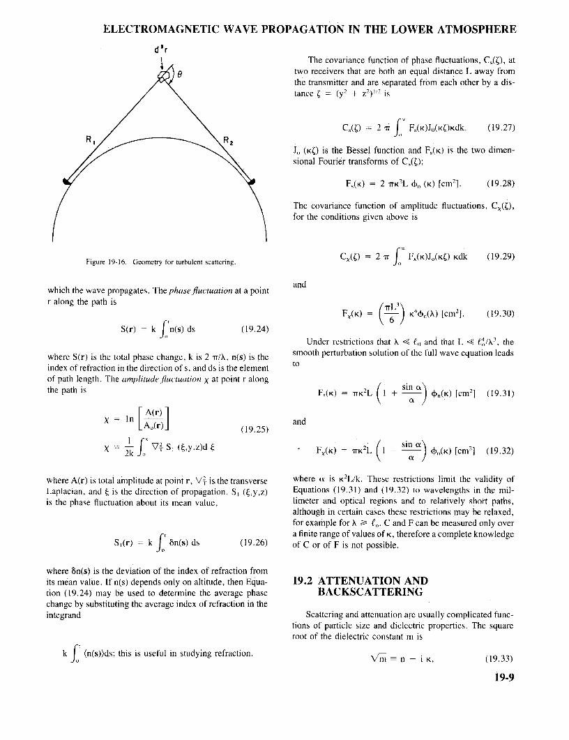
ELECTROMAGNETIC WAVE PROPAGATION IN THE LOWER ATMOSPHERE

d3rThe covariance function of phase fluctuations, Cs(), at

two receivers that are both an equal distance L away fromthe transmitter and are separated from each other by a dis-tance ( = (y2

+ Z2)1/2 is

/Cs() = 2 r I Fs(K)Jo(KC)Kdk. (19.27)R R2

Jo (K ) is the Bessel function and Fs(K) is the two dimen-sional Fourier transforms of Cs( );

Fs(K) = 2 rK2L On (K) [cm2

]. (19.28)

The covariance function of amplitude fluctuations, Cx( ),for the conditions given above is

Figure 19-16. Geometry for turbulent scattering. Cx( ) 2 r f Fx(K)Jo(K ) Kdk (19.29)

which the wave propagates. The phase fluctuation at a point andr along the path is L

Fx(K) = 6) K 4()n(X) [cm 2 ]. (19.30)

S(r) = k n(s) ds (19.24)Under restrictions that X < lo and that L < l4o/A3, the

where S(r) is the total phase change, k is 2 r/X, n(s) is the smooth perturbation solution of the full wave equation leadsindex of refraction in the direction of s, and ds is the element toof path length. The amplitudefluctuation X at point r alongthe path is Fs(K) = rK2 L (1 + sin a ) On(K) [cm2] (19.31)

a

X =1n [A(r) andX Ao(r)](19.25)

X 2k V2T Sl (~,y,z)d Fx(K) = rK 2L I - sin a ) On(K) [cm2] (19.32)

where A(r) is total amplitude at point r, T2 is the transverse where a is K2L/k. These restrictions limit the validity ofLaplacian, and ~ is the direction of propagation. S1 (~,y,z) Equations (19.31) and (19.32) to wavelengths in the mil-is the phase fluctuation about its mean value, limeter and optical regions and to relatively short paths,

although in certain cases these restrictions may be relaxed,for example for X >= lo. C and F can be measured only overa finite range of values of K, therefore a complete knowledge

S1(r) = k J ~n(s) ds (19.26) of C or of F is not possible.

where ~n(s) is the deviation of the index of refraction fromits mean value. If n(s) depends only on altitude, then Equa- 19.2 ATTENUATION ANDtion (19.24) may be used to determine the average phase BACKSCATTERINGchange by substituting the average index of refraction in theintegrand Scattering and attenuation are usually complicated func-

tions of particle size and dielectric properties. The squareroot of the dielectric constant m isfok f (n(s))ds; this is useful in studying refraction.

m -- n - i K, (19.33)

19-9

CHAPTER 19

where n is the phase refractive index, K is the absorption 100.0 1000

index of the medium, and i is --1.In describing the properties of the particles, it is con-

venient to use the parameter K, defined by ICE

m - -WATER 7. 14- 2.89iK ± (19.34)

When the particles are small in comparison with thetransmitted wavelength, the Rayleigh approximation holds,and both the backscatter and the absorption are simple func- 001 2 4 6 8 10 12 14 16 18 20 22 24 26 28 30

tions of K. In this special case, backscatter is proportional rD/to [K]2, and attenuation is proportional to the imaginary partof minus K or (Im(-K)). Figure 19-17. Calculated values of the normalized (4o/rD 2 ) backscatter

cross section for water at 3.21 cm and 273 K and for iceFor water, [K]2 is practically constant and equals 0.93 at wavelengths from I to 10 cm.over a wide range of temperatures and wavelengths in thecentimeter range. Similarly [K]2 = 0. 176 for ice of normaldensity (0.917 g/cm2 ) and centimeter wavelengths. How- parameter , computed from the exact Mie equations. Theever, the imaginary part of K can vary significantly with normalized curve for ice is invariant with wavelength in thetemperature and wavelength, and both (K)2 and (Im( -K)) microwave region; the normalized curve for water is for avary with frequency at millimeter and submillimeter wave- temperature of 273 K and a 3.2,cm wavelength. As theselengths. Unfortunately, measurements have not been made figures show, ice spheres equal to or larger than the wave-at every possible combination of temperature and wave- length may scatter more than an order of magnitude greaterlength, and there is no single expression relating all the than water spheres of the same size. This is confirmed byvariables. To obtain the real and imaginary parts of K at experimental measurements.the desired temperature and wavelength, the reader. is re- Measurements at 5 cm wavelength indicate that the back-ferred to the computer program written by Ray [1972], ascorrected by Falcone et al. [1979]. This program interpolatesbetween measured values.

ICE m = 1.78-.0024i19.2.1 Backscattering and Attenuation

Cross Sections

The echo power returned by a scattering particle is pro-portional to its backscattering cross section, a. The powerremoved by an attenuating particle is proportional to thetotal absorption cross section, Qt. The size parameter (elec-trical size) is rD/X; D is the particle diameter and X theWavelength of the incident radiation. When the diameter ofthe scattering or attenuating particle is small with respectto X, the backscattering and total absorption cross sectionsmay be expressed with sufficient accuracy by the Rayleighapproximation.

For spherical particles, if D/X < 0.2,WATER m = 7.14 -2.89i

o = r5[K]2D6 [cm2] (19.35)0.01

0 2 3 4rD/ X

For particles with rD/X > 0.2, a should be computed from r D/Xthe equations of the Mie theory of scattering [Battan, 1959]. Figure 19-18. Calculated values of the normalized (4a/rD

2) backscatter

Figures 19-17 and 19-18 show normalized backscattering cross section for water at 3.21 cm and 273 K and for icecross section (4a/rD 2 ) for ice and for water versus the size at wavelengths from I to 10 cm. (Detail of Figure 19-17)

19-10

ELECTROMAGNETIC WAVE PROPAGATION IN THE LOWER ATMOSPHERE

scattering of so-called "spongy" hail (a mixture of ice and is useful to express Z as a function of either the precipitationwater) is 3 to 4 dB above that of the equivalent all-water rate R or the mass of liquid water (or water equivalent ofspheres and at least 10 dB above that of the equivalent solid the ice content) M. The returned radar signal can then beice spheres [Atlas et al., 1964]. Because of the variabilities related to Z, and through Z to R or M. Numerous Z-R andof sizes, shapes, and liquid water content of hail, no general Z-M relations have been proposed. They vary geographi-rules concerning backscattering and attenuation cross sec- cally, seasonally, and by type of precipitation.tions for hail can be made. As a first approximation, how- The following Z-R relations are typical of those mostever, the ice curve of Figures 19-17 and 19-18 may be used. often found in the literature:

For spherical particles, if rD/X < 0.1,

Z = 200 R16 widespread stratiform rain

TD Im (-K) + 2a [cm2 ]. (19.36) Z = 110 R1.47 drizzle

Z = 460 R1.61 thunderstorm

When rD/X > 0.1, Q1 must also be computed from the Z = 145 R1.64 orographicexact Mie equations. Several computer programs are avail-able to compute the total attenuation caused by any distri- Z = 314 R1.42 monsoonbution of water and/or ice particles. [See, for example,Falcone et al., 1979.] The scattering properties of snow are complicated by

the many forms in which snow can occur, either as singleice crystals or aggregates of such crystals. The followingrelationships are reasonable averages of observations:

19.2.2 ReflectivityZ = 500 R' 6 for single crystals

The average echo power returned by a group of randomlydistributed scattering particles is proportional to their re-flectivity n. Reflectivity is defined as the summation of the andbackscatter cross sections of the particles over a unit volume:

n = Ea. When the backscattering particles are spheres and Z = 2000 R2.0 for aggregatesare small enough with respect to wavelength so that theRayleigh approximation can be used (that is, rD/X < 0.2), where R is the snowfall rate in millimeters of water perthe reflectivity is proportional to the radar reflectivity factor hour.Z which is the summation over a unit volume of the sixth Measurements by Boucher [1981] relating the reflectiv-power of the particle diameters, Z = E D6 . Summation ity to the rate of snow accumulation suggest that a relationover a unit volume of Equation (19.35) gives of the form

= K2 = Z x l0 -' 2 [cm- '] (19.37) Z = A S 20

where S is the snowfall rate in millimeters of snow per hour,for Z in conventional units of mm6 and m-3 and X in cen- gives good agreement between measured radar reflectivitytimeters. and measured snowfall accumulation. Boucher found that

When the particles are larger than Rayleigh size or com- A varied between 6 x 10-3 to 2 x 10-2 when S was ex-posed of ice or water-ice mixtures, it is common practice pressed in millimeters per hour. This variability is due toto measure the radar reflectivity and express it in terms of the variability of the density of snow, which ranges overan equivalent reflectivity factor Ze. Substituting [K]2 = 0.93 an order of magnitude.(water at normal atmosphere temperature, wavelength in the Clouds composed of water particles scatter very poorlycentimeter range) in Equation (19.38) at centimeter wavelengths, due to the relatively small size

of the water droplets. High-power radars operating at mil-Ze = 3.5 x 109 X4 n (mm6 m-3 ). (19.38) limeter wave lengths can detect waterclouds at short ranges.

An empirical Z-M relation for water clouds is

Thus, Ze is simply the ED6 required to obtain the observedsignal, if all the drops were acting as Rayleigh scatterers. Z = 0.048M2

Because Z is a meteorological parameter that dependsonly on the particle size distribution and concentration, it where M, the water content, is in grams per cubic meter.

19-11

Table 19-1. Attenuation (db/km) at 293 K.

Precipitation Wavelength (cm)

Rate (mm/h) 0.03 0.05 0.1 0.15 0.2 0.25 0.3 0.5 0.8 1.0 2.0 3.0 5.0 6.0 15.0

0.25 0.867 0.900 0.874 0.773 0.656 0.539 0.434 0.179 0.0634 0.0381 0.685 0.231 0.657 0.434 0.631x l0- 2 x 10-2 x 10-3 x 10- 3 x 10- 4

1.25 2.31 2.43 2.51 2.41 2.22 1.99 1.74 0.919 0.374 0.232 0.0449 0.0134 0.304 0.191 0.249X 10-2 X 10- 2 x 10- 1

2.50 3.51 3.71 3.90 3.83 3.63 3.34 3.01 1.77 0.783 0.497 0.104 0.0311 0.618 0.374 0.454X 10- 2 X 10-2 X 10-3

5.00 5.35 5.65 6.01 6.02 5.83 5.49 5.08 3.29 1.60 1.05 0.239 0.0750 0.0132 0.758 0.829X 10 2 X 10- 3

12.50 9.35 9.86 10.59 10.80 10.69 10.33 9.81 7.13 3.94 2.70 0.698 0.245 0.0399 0.0209 0.186x 10

- 2

25.00 14.27 15.03 16.18 16.67 16.70 16.38 15.81 12.36 7.51 5.38 1.52 0.591 0.100 0.0488 0.348x 10- 2

50.00 21.78 22.90 24.68 25.61 25.89 25.70 25.14 20.89 13.87 10.37 3.23 1.38 0.265 0.124 0.661x 10- 2

100.00 33.22 34.85 37.55 39.18 39.84 39.96 39.50 34.54 24.83 19.40 6.66 3.09 0.706 0.338 0.0128150.00 42.48 44.51 47.93 50.16 51.10 51.54 51.22 45.94 34.46 27.59 10.06 4.86 1.24 0.613 0.0190

Table 19-2. Temperature correction factor for representative rains. WAVELENGTH (cm

Precipitation Temperature (K)Rate Wavelength 30 3mm/h cm 273 283 293 303 313

0.03 1.0 1.0 1.0 1.0 1.00.1 0.99 0.99 1.0 1.01 1.02

0.25 0.5 1.02 1.01 1.0 1.0 1.01.25 1.09 1.02 1.0 1.0 0.99 10-23.2 1.55 1.25 1.0 0.81 0.65

10.0 1.72 1.29 1.0 0.79 0.64

0.03 1.0 1.0 1.0 1.0 1.00.1 1.0 1.0 1.0 1.0 1.01

2.5 0.5 1.01 1.01 1.0 0.99 0.981.25 0.95 0.96 1.0 1.05 1.103.2 1.28 1.14 1.0 0.86 0.72

10.0 1.73 1.30 1.0 0.79 0.64

0.03 1.0 1.0 1.0 1.0 1.00.1 1.0 1.0 1.0 1.0 1.01

12.5 0.5 1.02 1.01 1.0 0.99 0.97 10-31.25 0.96 0.97 1.0 1.04 1.073.2 1.04 1.03 1.0 0.95 0.88

10.0 1.74 1.30 1.0 0.79 0.63

0.03 1.0 1.0 1.0 1.0 1.00.1 1.0 1.0 1.0 1.0 1.01

50.0 0.5 1.02 1.01 1.0 0.98 0.971.25 0.99 0.99 1.0 1.02 1.043.2 0.91 0.96 1.0 1.01 1.01

10.0 1.75 1.31 1.0 0.78 0.62

0.03 1.0 1.0 1.0 1.0 1.0 10-40.1 1.0 1.0 1.0 1.0 1.01 3 10 30

150.0 0.5 1.03 1.01 1.0 0.98 0.97 FREQUENCY(GHz)1.25 1.01 1.0 1.0 1.0 1.013.2 0.88 0.95 1.0 1.04 1.06 Figure 19-19. Theoretical attenuation due to snowfall of 10 mm of water

10.0 1.72 1.31 1.0 0.78 0.62 content per hour as a function of wavelength and temper-ature.

19-12

ELECTROMAGNETIC WAVE PROPAGATION IN THE LOWER ATMOSPHERE

19.2.3 Attentuation by Precipitation Table 19-3. Attenuation due to molecular oxygen at a temperature of293 K and a pressure of l-atmosphere.

Attenuation by rain is a function of drop size distribu- Wavelength Attenuationtion, temperature and wavelength. Theoretical computa-tions [Dyer and Falcone, 1972] indicate that for a given (cm) (dB km)rainfall rate, wavelength and temperature, the variations 10.0 6.5 x 10-3in drop size distribution can cause deviations in average at- 7.5 7.0 x 10-3tenuation of between 4% and 33%. For comparison, meas- 3.2 7.2 x l0- 3

ured attenuations are accurate to no more than ± 20% in 1.8 7.5 x 10-3general. 1.5 8.5 x 10-3

Table 19-1 gives the theoretical attenuation, for a wide 1.25 1.4 x 10-2range of rainfall rates and wavelengths, assuming a constant 0.8 7.5 x 10 2temperature of 293 K and an exponential distribution of 0.7 1.9 x 100drop sizes. Table 19-2 gives the attenuation correction factorfor a range of rain rates and temperatures.

Figure 19-19 shows the theoretical maximum attenua-tion coefficients assuming a maximum snowfall rate 10 mm ample, Falcone et al., 1979] to calculate the total attenu-of water per hour. Because snowfall rates seldom exceed ation at any frequency, for any input atmospheric condition.3 mm of water per hour, attenuation due to snow should Figure 19-20 is an example of the output from one suchgenerally be one-third or less the value. program.

The solid line (curve A) shows the attenuation at stand-

19.2.4 Total Attenuation Table 19-4. Correction factors for oxygen attenuation.

In addition to attenuation caused by precipitation par- Temperatureticles, microwave and millimeter wave transmission is af- (K) Correction Factor*fected by atmospheric gases, water vapor, and cloud par-ticles. Table 19-3 gives the attenuation as a function of 293 1.00 p 2

wavelength for molecular oxygen at 293 K, and Table 273 1.19 p 2

19-4 gives correction factors for temperature differing from 253 1.45 p 2

293 K. Table 19-5 does the same for water vapor atten- 233 1.78 p 2

uation. Computer programs have been written [see, for ex- *P is pressure in atmospheres.

Table 19-5. Water-vapor attenuation in dB per kilometer.*

Wavelength Temperature(cm) 293 K 273 K 253 K 233 K

10 7 PW x 10- 5 8 PW x 10-5 9 PW x l0-5 10 PW X 10- 5

5.7 2.4PW x 10- 4 2.7 PW x 10-4 3.0 PW x 10-4 3.4 PW x 10-4

3.2 7 PW x 10-4 8 PW x 10-4 9 PW x 10- 4 10 PW x 10-4

1.8 4.3 PW x l0 - 3 4.8 PW x l0 - 3 5.0 PW X l0 - 3 5.4 PW x 10-3

1.24 2.2 PW x 10 2 2.33 PW x 10-2 2.46 PW x 10- 2 2.61 PW x 10-2

0.9 9.5 PW x 10- 3 1.04 PW x 10- 2 1.14 PW x 10- 2 1.26 PW x 10 2

*P is pressure in atmospheres and W is water-vapor content in grams per cubic meter.

19-13

CHAPTER 19

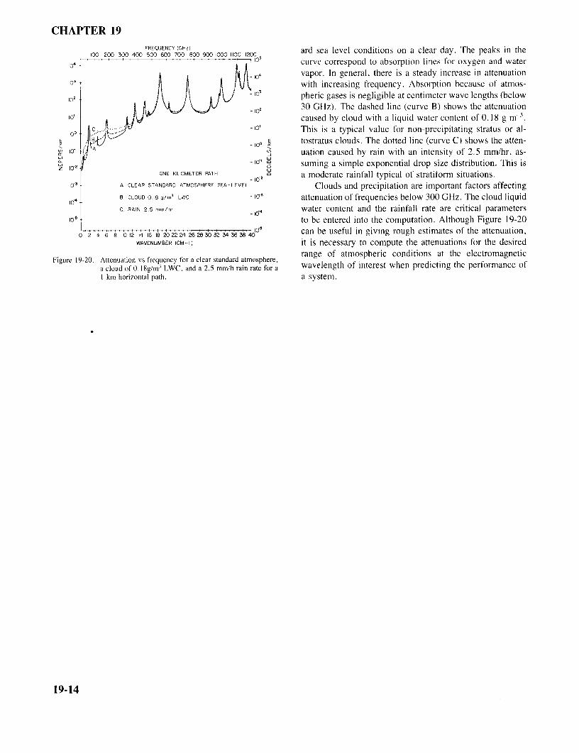
FREQUENCY ard sea level conditions on a clear day. The peaks in the100 200 300 400 500 600 700 800 900 1000 1100 120010

4 curve correspond to absorption lines for oxygen and watervapor. In general, there is a steady increase in attenuationwith increasing frequency. Absorption because of atmos-

pheric gases is negligible at centimeter wave lengths (below30 GHz). The dashed line (curve B) shows the attenuationcaused by cloud with a liquid water content of 0.18 g m-3.

This is a typical value for non-precipitating stratus or al-tostratus clouds. The dotted line (curve C) shows the atten-uation caused by rain with an intensity of 2.5 mm/hr, as-suming a simple exponential drop size distribution. This is

ONE KILOMETER PATH a moderate rainfall typical of stratiform situations.10-

3A CLEAR STANDARD ATMOSPHERE SEA-LEVEL Clouds and precipitation are important factors affectingB. CLOUD 0.18 g/m

3LWC 10-3 attenuation of frequencies below 300 GHz. The cloud liquid

C RAIN 2.5 mm/hr 10-4 water content and the rainfall rate are critical parametersto be entered into the computation. Although Figure 19-20

0 2 4 6 8 10 12 14 16 18 202224 26 28 30 32 34 36 38 40 can be useful in giving rough estimates of the attenuation,WAVENUMBER (CM-1) it is necessary to compute the attenuations for the desired

range of atmospheric conditions at the electromagneticFigure 19-20. Attenuation vs frequency for a clear standard atmosphere,

a cloud of 0.18g/m3 LWC, and a 2.5 mm/h rain rate for a wavelength of interest when predicting the performance of1 km horizontal path. a system.

19-14

ELECTROMAGNETIC WAVE PROPAGATION IN THE LOWER ATMOSPHERE

REFERENCES

Atlas, D., K.R. Hardy, J. Joss, "Radar Reflectivity of Storms Gunn, K.L.S. and T.W.R. East, "The Microwave Prop-Containing Spongy Hail,"J. Geophys. Res., 69: 1955, erties of Precipitation Particles," Quart. J. Roy. Mete-1964. orol. Soc., 80:522, 1954.

Battan, L.J., Radar Meteorology, The University of Chi- Hardy, K.R. and I. Katz, "Probing the Clear Atmospherecago Press, p. 33, 1959. with High Power High Resolution Radars," PROC. IEEE,

Bean, B.R. and E.J. Dutton, Radio Meteorology, Dover, 57:468, 1969.Mineola, New York, 1968. Hufnagle, R.E. and N.R. Stanley, "Modulation Transfer

Boucher, R.J., "Determination by Radar Reflectivity of Short- Function Associated with Image Transmission ThroughTerm Snowfall Rates During a Snowstorm and Total Turbulent Media," J. Opt. Soc. Am., 54: 52, 1964.Storm Snowfall," Proceedings 20th Conference on Ra- Hufnagle, R.E., "Variations of Atmospheric Turbulence,"dar Meteorology, Boston, Nov 30-Dec 3, 1981, Amer- Digest of Technical Papers, Topical Meeting on Opticalican Meteorology Society, Boston, Mass., 1981. Propagation Through Turbulence July 9-11, 1974. Op-

Brown, J.H., R.E. Good, P.M. Bench, and G. Foucher, tical Society of America, Washington, D.C., 1974."Sonde Experiments for Comparative Measurements of Liebe, H.J., Atmospheric Water Vapor p. 143-202, editedOptical Turbulence," AFGL GR-82-0079, ADA118740, by A. Deepak, T.D. Wilkinson, and A.L. Schemelte-1982. kopf, Academic Press, New York, 1980.

Crane, R., "Monostatic and Bistatic Scattering from Thin Medhurst, R.G., "Rainfall Attenuation of Centimeter Waves:Turbulent Layers in the Atmosphere," Lincoln Lab. Tech. Comparison of Theory and Measurement," IEEE Trans.Note 1968-34, ESD-TR-68267, 1968. Antennas and Propagation; AP-13:550, 1965.

Crane, R.K., "A Review of Radar Observations of Tur- Ottersten, H., "Radar Backscatter from the Turbulent Clearbulence in the Lower Statosphere," Radio Sci., 15: 177, Atmosphere," Radio Sci.; 4:1251, 1969.1980. Ray, P.S., "Broadband Complex Refractive Indices of Ice

Cunningham, R.M., "Cumulus Climatology and Refractive and Water," Appl. Opt., 11: 1836-1844, 1972.Index Studies II," Geophys. Res. Papers, No. 51, AFCRL, Staras, H. and A.D. Wheelon, "Theoretical Research on1962. Tropospheric Scatter Propagation in the United States

Dewan, E.M., "Optical Turbulence Forecasting: A Tuto- 1954-1957," IEEE Trans. Antennas and Propagation,rial," AFGL TR-80-0030, ADA086863, 1980. AP-7:80, 1959.

Dyer, R.M. and V.J. Falcone, "Variability in Rainfall Rate- Strohnbehn, J.W., "Line of Sight Wave Propagation ThroughAttenuation Relations," Prep, 15 Radar Meteorology the Turbulent Atmosphere," PROC. IEEE, 56:1301,Conference, p. 353, 1972. 1968.

Edlen, B., "Dispersion of Standard Air," J. Opt. Soc. Am., Tatarski, V.I., Wave Propagation in a Turbulent Media,43:339, 1953. Chapters 3, 6 and 7, McGraw-Hill, New York, 1961.

Falcone, V.J., L.W. Abreu, and E.P. Shettle, "Atmospheric Tatarski, V.I., The Effects of the Turbulent Atmosphere onAttenuation of Millimeter and Submillimeter Waves: Wave Propagation, National Science Foundation, TT-Model and Computer Code," AFGL TR-79-0253, 68-50464, 1971.ADA084485 1979. VanZandt, T.E., K.S. Gage, and J.M. Warnock, "An Im-

Gage, K.S., T.E. VanZandt, and J.L. Green, "Vertical proved Model for the Calculation of Profiles of C2 nandProfiles of Cn2 in The Free Atmosphere: Comparison of E in the Free Atmosphere from Background Profiles ofModel Calculations with Radar Observations," 18th Wind, Temperature and Humidity," Proceedings 20thConference on Radar Meteorology, Atlanta, GA, 28-31 Conference on Radar Meteorology, Boston, Mass., NovMarch 1978, American Meteorology Society, Boston, 30-Dec 3, 1981, American Meteorology Society, Bos-Mass., 1978. ton, Mass., 1981.

Good, R.E., B. Watkins, A. Quesada, J.H. Brown, and G.Lariot, "Radar and Optical Measurements of Cn2 ," App.Optics, 21:2929, 1982.

19-15