Embed Size (px)
Citation preview
Modal Congestion Management Strategies and the Influence on Operating Characteristics of
Urban Corridor
A thesis submitted in fulfilment of the requirements for the degree of Master of Engineering
Kaniz Fatima
Bachelor of Engineering (Civil Engineering)
School of Civil Environmental and Chemical Engineering
College of Science Engineering and Health
RMIT University
October, 2015

i
Declaration
I certify that except where due acknowledgement has been made, the work is that of
the author alone; the work has not been submitted previously, in whole or in part, to
qualify for any other academic award; the content of the thesis/project is the result of
work which has been carried out since the official commencement date of the
approved research program; any editorial work, paid or unpaid, carried out by a third
party is acknowledged; and, ethics procedures and guidelines have been followed.
Kaniz Fatima
19/10/2015
ii
Acknowledgements
I would like to take this opportunity to express my deepest appreciation
and gratitude to my supervisor, Dr. Sara Moridpour, for her endless
support and beneficial discussions throughout my candidature at RMIT
University. It has been a great pleasure and privilege to work with her
and to benefit from her rich knowledge and experience. I also thank my
second supervisor Dr. Nira Jayasuriya for her kind help and support
when I faced difficulties.
I would like to thank VicRoads for providing necessary support. Many
thanks to my colleagues and former postgraduate students whose
friendship, companionship and fruitful discussion have created a fun
environment to learn and grow. I am also thankful to school management
staffs for their full support during my candidature. I am grateful to Mark
Besley, Rahmi Akcelik and their team from SIDRA solution for their
help during my simulation process with software and Dr Alex McKnight
who assisted by proofreading the final version of the thesis.
I wish to express my deepest gratitude to my parents, to whom this thesis
is dedicated. You’ve borne me, raised me, taught me and loved me,
continuously and unconditionally. To my husband and daughter, thank
you for sharing this journey. During this journey you two were always
positively supportive and understood the excitement, frustration, despair
and joy I went through. I am forever grateful. Above all, I am forever
grateful for to our Almighty, to whom I was shown his everlasting grace
and faithfulness, giving me the strength to complete this research.
iii
Abstract
In recent years, traffic congestion has become a major problem in
transportation networks particularly in peak periods. The congestion problem
has become worse in large cities, particularly in the CBDs over the last few
decades and the problem intensifies every year. Traffic congestion results in
longer travel times, larger delays, more fuel consumptions and more emission.
Australian Bureau of Infrastructure, Transport and Regional Economics
estimates wastage of a total of $9.4 billion as the social cost of congestion for the
year 2005 in the major Australian cities and the cost will be around that the
avoidable social costs of congestion will be more than doubled by 2020.
Traffic congestion problem in Australia may be the consequence of many
factors. Congestion is generally worse in inner suburbs than outer areas. A
large number of commuters travel to/from work and school on same time
intervals representing the most significant contributors of congestion. Rapid
increases in population and number of cars are the key reasons of traffic
congestion. Other key causes of congestion relating to both supply and demand
sides include under-pricing of road use, lack of proper road infrastructure
design/operation, travel demand growth and inadequate public transport
alternatives. Traffic congestion is a consequence of all these factors. Therefore,
effective demand management can reduce traffic congestions in urban areas.
Urban travel demand is growing rapidly in almost all main cities while sources
of providing enough supply in the form of new road infrastructure or public
transport are limited. Different approaches can be applied to manage traffic
congestion. These strategies can be defined as construction of new
infrastructure, congestion pricing management strategies and modal
management strategies. However, apply modal congestion strategies is
economical for case study (Melbourne corridor/intersection).
The case study for this research is a corridor in Melbourne metropolitan area.
The corridor starts from intersection of Manningtree Road and Power Street to
Abstract iv
intersection of Princes Street and Beatrice Street (M21, Mel ways Ref: 45,
C11- Street Directory).
This research intends to propose a solution to reduce traffic congestion and
consequently traffic delay for a congested corridor in Melbourne metropolitan
area. To achieve this, a number of strategies are introduced and their influence
on traffic congestion is evaluated. Dedicated bus/tram lane, Bus/tram stop
location change, Parking restriction, Bicycle lane restriction, Passenger car
movement restriction, Lane configuration, advanced green signal and extended
green signal will be applied to reduce congestion strategies.
This research models the selected Melbourne corridor using SIDRA software
with real time datasets (collected from VicRoads, Site Survey, Google maps,
Bus network and Tram network data). Different parameters of the data sets
such as speed limit, traffic volume (number of tram, bus and passenger cars),
signal timing (red, yellow and green times), number of lanes, direction of lane
traffic movement and parking restrictions are collected from data sources.
Datasets are used to model each intersection of the study corridor. The model
of each intersection is calibrated and validated with collected datasets from site
survey. After validation the intersections are added as a network or corridor.
The corridor also needed to be calibrated and validated using collected site
survey datasets. The variables used for calibration are traffic blockage, delay
times, average speeds and queue lengths which are experienced by different
modes of transport. After the model validation, modal management strategies
are applied to the corridor to reduce traffic congestion. Three main parameters
including average speed, delay time and queue length experienced by different
modes of transport are compared to identify strategies to control congestion.
Modifying the order of signal phases and cycle length is the best simulated
strategy for this corridor. Besides that applying parking restriction to this
corridor during peak period also reduces congestion.
v
List of Publications
Journals
FATIMA, K. & MORIDPOUR, S. Multimodal congestion management
strategies at urban intersections-Case study Melbourne. Journey of Land
Transport Authority (LTA) Singapore (Submitted full manuscript to Land
Transport Authority, Singapore).
Conferences
FATIMA, K. & MORIDPOUR, S. (2015). Micro simulation model analysis-
Case study of urban corridor. Asia-Pacific World Congress on Engineering, 4-
5th
May 2015, Plantation Island, Fiji (Abstract and full manuscript accepted).
FATIMA, K. & MORIDPOUR, S. (2015). Micro simulation model of modal
congestion management strategies: A case study of SIDRA analysis. Road
Safety & Simulation International Conference, October 6-8, 2015, Orlando,
Florida, USA (Abstract accepted and full manuscript submitted).
FATIMA, K. & MORIDPOUR, S. (2015). Evaluation of modal congestion
management strategies at Melbourne corridor. Australasian Transport Research
Forum, 30 September to 2 October 2015, Sydney, Australia (Abstract accepted
and full paper submitted).
vi
Table of Contents
Chapter 1 Introduction
1.1 Background………………...………………………………….…………..1
1.2 Strategies for Congestion Management………………………….………..2
1.2.1 Infrastructure expansion……………………………….…………..3
1.2.2 Congestion pricing management…………………...……………...3
1.2.3 Modal congestion management……………………………………4
1.3 Aims and Objectives…………………………………………...………….5
1.4 Research Structure……………………………………………………...…6
Chapter 2 Background of Research
2.1 Introduction………………………………………………………………...8
2.2 Strategies to Control congestion……………………………………………8
2.2.1 Infrastructure expansion……………………………………………..9
2.2.2 Congestion pricing management…………………………………...10
2.2.3 Modal congestion management…………………………………….12
2.3 Limitation of Existing Studies……………………………………………17
2.4 Research Contribution…………………………………………………….18
2.5 Summary……………………………………………………………..…...19
Chapter 3 Research Framework
3.1 Introduction……………………………………………………………….20
3.2 Study Corridor…………………………………………………………….20
3.2.1 Area of Study……………………………………………………….20
3.2.2 Lane Approaches at Selected Intersections………………………...22
3.3 Methodology……………………………………………………………...23
3.4 Datasets…………………………………………………………………...24
3.4.1 VicRoads SCATS data…………………………………………….24
3.4.2 Survey…….………………………………………………………...25
Table of Contents vii
3.4.3 Google Maps……………………………………………………….26
3.5 Summary of Various Datasets…………………………………………….26
3.6 Summary………………………………………………………………….29
Chapter 4 Model Development
4.1 Introduction……………………………………………………………….30
4.2 SIDRA Intersection……………………………………………………….30
4.3 Corridor Modelling………………………………………………………..30
4.3.1 Intersection of Denmark Street/ High street/ Princess Street/ Studley
Street/ High Street South (Site 3662)………………………………….…31
4.3.2 Intersection of Denmark Street/ Wellington Street (Site 3663)……37
4.3.3 Intersection of Denmark Street/ Stevenson Street (Site 1190)……..39
4.3.4 Intersection of Denmark Street/ Power Street/ Barker Road (Site
3002)……………………………………………………………………...42
4.4 Output Results…………………………………………………………….45
4.5 Intersection Calibration…………………………………………………...48
4.6 Corridor Model and Calibration…………………………..........................52
4.7 Summary………………………………………………………………….53
Chapter 5 Applied Strategies
5.1 Introduction……………………………………………………………….54
5.2 Strategies applied to reduced congestion…………………………………54
5.3 Application of strategies to the case study corridor………………………55
5.3.1 Intersection of Denmark Street/ High street/ Princess Street/ Studley
Street/ High Street South (Site 3662)…………………………………….55
5.3.2 Intersection of Denmark Street/ Wellington Street (Site 3663)…....66
5.3.3 Intersection of Denmark Street/ Stevenson Street (Site 1190)……..69
5.3.4 Intersection of Denmark Street/ Power Street/ Barker Road (Site
3002)……………………………………………………………………...71
5.4 Results and Discussion……………………………………………………77
5.5 Summary………………………………………………………………….81
Table of Contents viii
Chapter 6 Conclusion and Future Research
6.1 Conclusion………………………………………………………………...82
6.2 Research Contribution…………………………………………………….82
6.3 Future Research Directions……………………………………………….83
References........................................................................................................84
Appendix A......................................................................................................94
Appendix B…………………………………………………………………...97
ix
List of Figures
Figure 1.1: Average unit costs of congestion for Australia metropolitan
areas……………………………………………………………………………...…….2
Figure 1.2: Research Structure Flowchart………………………………..…………….6
Figure 2.1: Strategies available for traffic congestion management…………………...8
Figure 2.2: Classification of Modal Congestion Management Strategies………...….12
Figure 2.3: Space Priorities, Sao Paulo (Google image)……………………...............14
Figure 2.4: Simplified Structure of IBL……………………………………..………..15
Figure 2.5: Signal time control procedures…………………………………...............16
Figure 3.1: Google Map for Case Study Corridor……………………………………21
Figure 4.1: Flow Chart of SIDRA (SIDRA Software)……………….……………….31
Figure 4.2: Intersection Layout of Site 3662…………………………………………32
Figure 4.3: Approach Direction of Site 3662………………………………………....33
Figure 4.4: Intersection Layout of Site 3663………………………………………....37
Figure 4.5: Approach Direction of Site 3663…………………………………………38
Figure 4.6: Intersection Layout of Site 1190……………………….………………...40
Figure 4.7: Approach Directions of Site 1190……………………………………......40
Figure 4.8: Intersection Layout of Site 3002………………………………...……….42
Figure 4.9: Approach Direction of Site 3002…………………………………………43
Figure 4.10: LOS Layout of Site 3662……………………………………….……….46
Figure 4.11: LOS Layout of Site 3663………………………………………………..47
Figure 4.12: LOS Layout of Site 1190………………………….…………………..47
Figure 4.13: LOS Layout of Site 3002………………………………………………..48
Figure 4.14: Case Study Corridor Layout…………………………………………….53
Figure 5.1: Movement restriction from High Street south towards Princess Street,
3662……………………………………………………………………………...……56
List of Figures x
Figure 5.2: Movement restriction from High Street south towards Princess Street,
3662………………………………………………………………………………...…56
Figure 5.3: Movement restriction from Princess Street towards High Street south,
3662……………………………………………………………………...……………57
Figure 5.4: Movement restriction from High Street south towards Princess Street; from
Denmark Street towards High Street South; from Princess Street towards High Street
south and from High Street lane 1 towards Studley Street,
3662…………………………………………………………………………………...57
Figure 5.5: Movement restriction from High street south towards Princess Street and
from High Street lane 1 towards Studley Street, 3662………………………………..58
Figure 5.6: Movement restriction from High Street south towards Princess Street and
from Denmark Street towards High Street south, 3662………………………………58
Figure 5.7: Movement restriction from Princess Street and from Princess Street
towards High Street south, 3662……………………………………………………...59
Figure 5.8: Movement restriction from High Street lane1 towards Studley and from
Denmark Street towards High Street south, 3662…………………………………….59
Figure 5.9: Movement restriction from High street lane1 towards Studley Street and
from Princess Street High Street south, 3662……………………………………..….60
Figure 5.10: Movement restriction from Denmark Street towards High Street south
and from Princess Street towards High Street south, 3662………………………..….60
Figure 5.11: Lane configuration to Studley Street, 3662……………………………..61
Figure 5.12: Bus/Tram dedicated lane, 3662…………………………………………61
Figure 5.13: Bicycle lane restriction on Princess Street, 3662……………………….62
Figure 5.14: Bicycle lane restriction on High Street, 3662…………………………...62
Figure 5.15: Tram stop relocation, 3662……………………………………………...63
Figure 5.16 Original signal phase (E,F,D,C,A,B,G), 3662…………………………...64
Figure 5.17 Changed signal phase (A,B,E,C,D,F,G), 3662…………………………..65
Figure 5.18 Lane Configuration, 3663………………………………………………..66
Figure 5.19 Original signal phase (A, B, B2, C, D, F, E1, E2), 3663………………...67
Figure 5.20 Changed signal phase (A, B, B2, C), 3663………………………………68
List of Figures xi
Figure 5.21 Changed signal phase (A, C, B, B2, D, F, E1, E2), 3663………………..69
Figure 5.22 Original signal phase (A, B), 1190………………………………………70
Figure 5.23 Changed signal phase (A, B, A1, B1), 1190……………………………..70
Figure 5.24 Changed signal phase (B, A, B1, A1), 1190……………………………..71
Figure 5.25 Lane 1 & 2 at High Street, 3662…………………………………………74
xii
List of Tables
Table 2.1: Comparison of different management strategies………………………….18
Table 3.1: Summary of Lane Approaches……………………………………………22
Table 3.2: Summary of Intersections Groupings……………………………..............26
Table 3.3: Summary of Vehicle Controller Time Settings…………………………...27
Table 3.4: Summary of Bus and Tram Operation through Corridor………………….27
Table 3.5: Summary of Intersection Geometries and Movements……………………28
Table 4.1: Summary of Approach Distance, Site 3662……………………………….32
Table 4.2: Summary of Basic Saturation Flow, Site 3662……………………………33
Table 4.3: Summary of Gap Acceptance Data, Site 3662……………………………34
Table 4.4: Summary of a Signal Cycle, Site 3662……………………………………35
Table 4.5: Summary of Signal Data, Site 3662……………………………………….36
Table 4.6: Summary of Approach Distance, Site 3663……………………………….37
Table 4.7: Summary of Basic Saturation Flow, Site 3663……………………………38
Table 4.8: Summary of Gap Acceptance, Site 3663………………………………….38
Table 4.9: Summary of Signal Data, Site 3663……………………………………….39
Table 4.10: Summary of a Signal Cycle Phase, Site 3663……………………………39
Table 4.11: Summary of Approach Distance, Site 1190……………………...............40
Table 4.12: Summary of Basic Saturation Flow, Site 1190………………………….41
Table 4.13: Summary of Gap Acceptance, Site 1190………………………………...41
Table 4.14: Summary of Signal Data, Site 1190……………………………………...41
Table 4.15: Summary of a Signal Cycle Phase, Site 1190……………………………42
Table 4.16: Summary of Approach Distance, Site 3002……………………………...43
Table 4.17: Summary of Basic Saturation Flow, Site 3002…………………………..43
Table 4.18: Summary of Gap Acceptance, Site 3002……………………………….44
Table 4.19: Summary Signal Data, Site 3002………………………………………...44
List of Tables xiii
Table 4.20: Summary of a Signal Cycle Phase, Site 3002……………………………45
Table 4.21: Parameter Calibration, Site 3662……………….………………………..49
Table 4.22: Parameter Calibration, Site 3663………………………………...............50
Table 4.23: Parameter Calibration, Site 1190……………………………….............51
Table 4.24: Parameter Calibration, Site 3002……………………………………….51
Table 4.25: Traffic Matrices Volumes………………………………………………52
Table 5.1: Output Parameter Summary for Applied Strategies (Intersection
3662)…………………………………………………………………………………72
Table 5.2: Output Parameter Summary for Applied Strategies (Intersection
3663)…………………………………………………………………………………75
Table 5.3: Output Parameter Summary for Applied Strategies (Intersection
1190)…………………………………………………………………………………76
Table 5.4: Summary of Network Output Parameter Comparison
(Strategy 1)……………………………………………………………………………78
Table 5.5: Summary of Network Output Parameter Comparison
(Strategy 2)……………………………………………………………………………79
Table 5.6: Summary of Network Output Parameter Comparison
(Strategy 1&2)………………………………………………………………………...80
Table 5.7: Summary of Network Output Parameter Comparison…………………….81
Table A1 Summary of Traffic Volume……………………………………………….95
Table A2 Summary of Intersection Geometries and Movements………….…………96
Table B1 Output Movement Summary Street, High Street, Studley Street, Princess
Street and High Street south………………………………………………………….98
Table B2 Output Movement Summary of intersection Denmark Street and Wellington
Street………………………………………………………………………………….99
Table B3 Output Movement Summary of intersection Denmark Street and Stevenson
Street………………………………………………………………………………...100
Table B4 Output Movement Summary of intersection Barker road, Power Street and
Denmark Street……………………………………………………………………101
1
Chapter 1
Introduction
1.1 Background
In recent years, traffic congestion has become a major problem in transport networks,
particularly in peak periods. Congestion has become worse in large cities, particularly
in Central Business Districts (CBDs) over the last few decades, and the problem
intensifies every year. Congestion results in longer travel times, larger delays, more
fuel consumption and more emissions. Time wasted in congestion has a huge cost for
society. The Texas Transport Institute (TTI) 2012 Urban Mobility Report reveals that
U.S.A commuters wasted $5.5 billion hours of time and fuel due to traffic congestion
in 2011. This is equal to the amount of time that business and individual taxpayers
spend lodging their tax applications.
In Australia, the Australian Bureau of Infrastructure, Transport and Regional
Economics (BTRE) preliminary study estimates wastage of a total of $9.4 billion as
the social cost of congestion for the year 2005 in the major Australian cities and the
cost will be doubled by 2020. This total is comprised of approximately $3.5 billion in
private time costs (losses from trip delay and travel time variability), $3.6 billion in
business time costs (trip delay plus variability), $1.2 billion in extra vehicle operating
costs, and $1.1 billion in extra air pollution damage costs. The national total is spread
over the capital cities, with Sydney showing the highest ($3.5 billion), followed by
Melbourne ($3.0 billion), Brisbane ($1.2 billion), Perth ($0.9 billion), Adelaide ($0.6
billion), Canberra ($0.11 billion), Hobart ($50 million) and Darwin ($18 million).
According to BTRE, the avoidable social congestion cost will be an estimated $20.4
billion by 2020. The average unit costs of congestion are forecast to rise by around 59
per cent over this period (from year 2005 to 2020) as average delays become longer,
Chapter 1. Introduction 2
congestion, become more widespread and the proportion of freight and service
vehicles increases. This is equivalent to a roughly 87 per cent increase in
(metropolitan average) per capita congestion costs between 2005 and 2020 (Transport
2007).
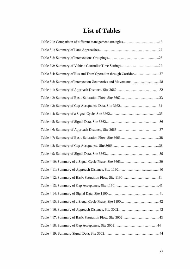
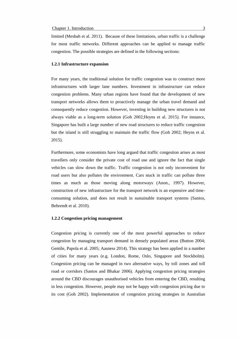
Figure 1.1 displays how the unit congestion costs in cents per passenger car unit per
kilometre, (PCU-km) vary between the capital cities. The rightmost columns of Figure
1.1 refer to weighted average values across all Australian metropolitan areas i.e.,
averaging the cost for all eight capitals across the vehicle kilometres travelled level.
Figure 1.1: Average unit costs of congestion for Australian metropolitan areas (Transport 2007).
Traffic congestion in Australia may be the consequence of many demand factors.
Congestion is generally worse in inner suburbs than outer areas, with travel to and
from work and school representing the most significant contributors. Rapid increases
in population and the number of cars are the key reasons for traffic congestion. Other
key causes are under-pricing of road use, lack of adequate road infrastructure
design/operation, growing demand for travel and inadequate public transport
alternatives. Therefore, effective demand management can reduce congestion.
1.2 Strategies for Congestion Management
Urban travel demand is increasing rapidly in almost all the main cities, while sources
to provide enough supply in the form of new road infrastructure or public transport are
0
2
4
6
8
10
12
14
Unit Cost (c/km) 2005
Unit Cost (c/km) 2020
Chapter 1. Introduction 3
limited (Mesbah et al. 2011). Because of these limitations, urban traffic is a challenge
for most traffic networks. Different approaches can be applied to manage traffic
congestion. The possible strategies are defined in the following sections:
1.2.1 Infrastructure expansion
For many years, the traditional solution for traffic congestion was to construct more
infrastructures with larger lane numbers. Investment in infrastructure can reduce
congestion problems. Many urban regions have found that the development of new
transport networks allows them to proactively manage the urban travel demand and
consequently reduce congestion. However, investing in building new structures is not
always viable as a long-term solution (Goh 2002;Heyns et al. 2015). For instance,
Singapore has built a large number of new road structures to reduce traffic congestion
but the island is still struggling to maintain the traffic flow (Goh 2002; Heyns et al.
2015).
Furthermore, some economists have long argued that traffic congestion arises as most
travellers only consider the private cost of road use and ignore the fact that single
vehicles can slow down the traffic. Traffic congestion is not only inconvenient for
road users but also pollutes the environment. Cars stuck in traffic can pollute three
times as much as those moving along motorways (Anon., 1997). However,
construction of new infrastructure for the transport network is an expensive and time-
consuming solution, and does not result in sustainable transport systems (Santos,
Behrendt et al. 2010).
1.2.2 Congestion pricing management
Congestion pricing is currently one of the most powerful approaches to reduce
congestion by managing transport demand in densely populated areas (Button 2004;
Gentile, Papola et al. 2005; Aasness 2014). This strategy has been applied in a number
of cities for many years (e.g. London, Rome, Oslo, Singapore and Stockholm).
Congestion pricing can be managed in two alternative ways, by toll zones and toll
road or corridors (Santos and Bhakar 2006). Applying congestion pricing strategies
around the CBD discourages unauthorised vehicles from entering the CBD, resulting
in less congestion. However, people may not be happy with congestion pricing due to
its cost (Goh 2002). Implementation of congestion pricing strategies in Australian
Chapter 1. Introduction 4
cities might be uneconomical and impractical. It is very difficult to change the
physical layout of cities and modify the geometric characteristics of streets (Ferrari
1989). To use toll systems for private cars people have to pay extra on a daily basis. In
Melbourne a zoning system is active for public transport. If congestion pricing
management applied to CBD travellers from distant zones, they would be charged
twice to travel during peak period (Armstrong-Wright 1986). Peak period is the main
travel period at morning (generally 7.30 am to 9.00am) and afternoon (generally 4.30
pm to 6.00 pm) for commuters.
1.2.3 Modal congestion management
Modal congestion management is another approach which focuses on space and time
allocation. Improving the public transport system motivates people to choose public
transport options as alternatives to driving. If traffic congestion increases, travellers
avoid it by changing their mode of transport, changing the route or their schedule
(Basso, Guevara et al. 2011; Wahlstedt 2011). If the alternative is attractive and time-
saving some drivers will shift mode, thereby reducing the level of congestion
equilibrium. Optimised travel options can therefore reduce delay for both travellers
who shift modes and those who continue driving. Many strategies have been proposed
to manage congestion by modal management. Some of these strategies involve
separate lanes, while others use signal priority.
Modal congestion management can also reduce delays caused by traffic. Modal
management strategies require the rearrangement of present congestion management
systems through the improvement of separate bus and tram lanes as well as advanced
or extended green signal time for public transport (bus and tram). Sao Paulo, Porto
Alegre, London and Melbourne are examples of cities that use space priority for buses
to control traffic congestion (Tyler 1991; Mesbah, Sarvi et al. 2011).
Melbourne and London also apply time priority at many intersections to reduce traffic
congestion. Modal management strategies are more cost effective than congestion
pricing management and developing infrastructures. The application of modal
management methods does not require extensive road infrastructure improvement.
Moreover, congestion has many facets, occurs in many different contexts and is
caused by different reasons. Therefore, there is no single approach to the management
of congestion. However, for Melbourne corridors/intersections, applying modal
Chapter 1. Introduction 5
management strategies is economical and time-saving (Litman 2012; Mahrous 2012;
Tirachini, Hensher et al. 2014).
1.3 Aims and Objectives
This research intends to propose a solution to reduce traffic congestion and
consequently traffic delay. To achieve this, a brief plan and a comparison of various
methods and strategies to deal with traffic congestion are described.
The broad aim of this research is to reduce traffic congestion in a particular corridor of
Melbourne by modal management strategies. A corridor is a network of intersections.
Melbourne operates the largest tram network in the world, and the tram system is a
popular and convenient mode of transport in the city. The case study corridor involves
almost every mode of transport, including trams, buses, cars, pedestrians and bicycles.
Consistent with this broad aim, the research objectives are identified as follows:
Identify different strategies which can be used to reduce traffic congestion and
delay for different modes of transport. Time/space priority for buses/trams,
parking restrictions during morning/afternoon peaks, changed signal phase and
cycle timing, restricted bicycle lanes during morning and afternoon peaks,
squeezing exit lanes to create additional lanes, restricting movement and
configuring exit lanes are some strategies applicable to various intersections or
the whole case study corridor.
Apply the strategies to a corridor in Melbourne as a case study. Corridors in
metropolitan areas generally comprise multiple transportation modes for
commuters, such as trains, buses, trams and private cars. During the morning
peak hour, commuters choose one of the available transportation modes to
travel through the corridor from rural/suburban living areas to urban working
areas.
Analyse and compare the influence of different strategies on traffic congestion
and delay of different modes of transport. The comparison of strategies will be
based on three different parameters: travel speed, queue distance and average
delay.
Chapter 1. Introduction 6
Propose efficient strategies to reduce congestion and travel delay based on the
simulation results and analysis. The proposed strategies will improve traffic
conditions for individual intersections and the network of intersections of the
case study corridor. The most effective strategies will be identified according to
travel speed, queue distance and average speed.
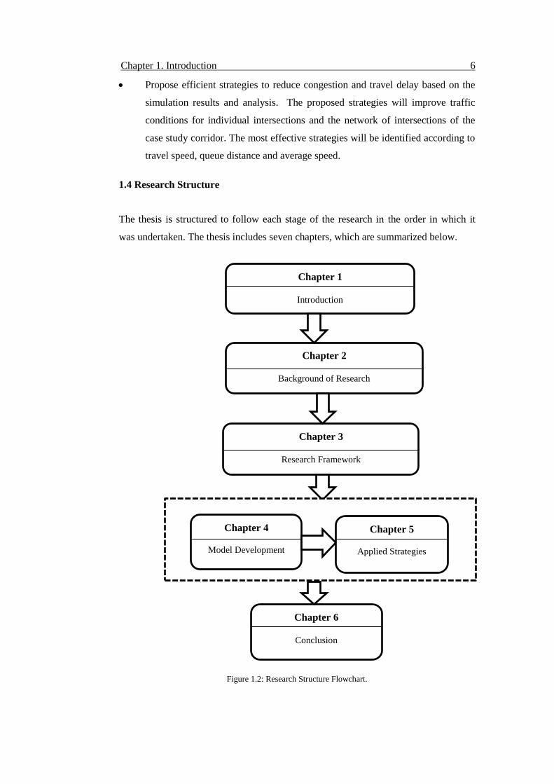
1.4 Research Structure
The thesis is structured to follow each stage of the research in the order in which it
was undertaken. The thesis includes seven chapters, which are summarized below.
Figure 1.2: Research Structure Flowchart.
Chapter 1
Introduction
Chapter 2
Background of Research
Chapter 3
Research Framework
Chapter 6
Conclusion
Chapter 4
Model Development
Chapter 5
Applied Strategies
Chapter 1. Introduction 7
In chapter 2, the existing strategies to control congestion are classified according to
characteristics. The modal congestion management strategies have been discussed
with major limitation of literature review. In addition, the strengths and weaknesses of
the each congestion control management strategies group is summarized.
This background of research is followed by an introduction of the study corridor
(chapter3). The methodology of thesis has been discussed in this chapter. Furthermore,
chapter 3 provides idea about type and classification of data sets.
Chapter 4 describes a detailed model development of the study corridor by using
software SIDRA. Micro-analytical software SIDRA has been introduced in this
chapter. This chapter detailed the modelling of each intersection and corridor
separately through individual input parameters. In addition individual software input
parameters with collected data also presented in this chapter.
Chapter 5 is the main chapter associated with results and discussion. Simulation
software SIDRA has been used to analysis .It discussed about the applied strategies on
individual intersection and the whole corridor. Following by chapter 4 the models
have developed and strategies applied to identify results. Chapter 5 also discussed the
results with justification.
Finally, chapter 6 summarizes the findings from this dissertation and discusses future
research direction.
8
Chapter 2
Background of Research
2.1 Introduction
This chapter provides a review of previous research and presents different strategies to
control congestion. Although modal congestion management is the main focus of the
present research, other strategies are reviewed for comparison. The chapter aims to
determine the contributions of traffic congestion research and identify the gaps in
previous research.
2.2 Strategies to Control Congestion
From literature review traffic congestion management can classify in different
sections. Infrastructure expansion, congestion pricing management and modal
congestion management are main three types of traffic congestion management
strategy. Congestion pricing management can also explain as toll zone and toll
roads/corridors. Other strategy modal congestion management is classified according
to space priority and time priority. Figure 2.1 represents a flow chart of congestion
management strategies based on the literature review.
Figure 2.1: Strategies available for traffic congestion management.
Traffic congestion management
Infrastructure expansion Modal congestion management
Congestion pricing management
Toll Zone Toll
roads/corridors Time priority Space priority
Chapter 2. Background of Research 9
2.2.1 Infrastructure expansion
Urban land redevelopment and reconstruction of a previously developed area is an
important component of city evolution (Wang, 2013). The traditional response to
congestion management was to invest in more road capacity (National Research
Council, 1993; Parry, 2002). However, the expansion of roads and tollways has been
found to be inefficient and expensive (Downs, 2004). Highway capacities are not
sufficient for the growth of vehicle miles travelled (Arnott and Small, 1994; Wang et
al., 2013). As a result, the congestion becomes worse. Similarly, the expansion of
public transportation infrastructure is not sufficient to reduce traffic congestion (Parry,
2002).
Generally, infrastructure improvement is useful to reduce traffic problems for a
smaller area such as the inner city or a segment of an expressway with heavy traffic
volumes (Verhetsel, 2001; Moriyama et al., 2011). A standard way of reducing
congestion in larger cities is to develop ring roads or loops to divert the traffic around
the city rather than through it (Elias and Shiftan, 2011). This bypass construction
changes the roadway system while improving traffic flows and travel times (Elias and
Shiftan, 2011). In relation to the effect on residential communities, some studies show
that bypasses have positive influences by reducing truck traffic, improving
accessibility and creating new opportunities to develop new areas (Collins and
Weisbrod, 2000; Leong, 2002; Elias and Shiftan, 2011). On the other hand, other
studies have found negative impacts, including sprawling low-density development,
and high environmental and infrastructure costs (Srinivasan and Kockelman, 2002).
For example, the construction of a northern bypass in Baton Rouge, Louisiana is an
infrastructure investment strategy aimed at congestion reduction within the area
(Antipova and Wilmot, 2012). The upgrading of existing network systems is more
efficient than the construction of bypasses. The existing road network system can
produce greater congestion relief than construction at approximately one-third of the
total cost. Upgrading existing networks also results in reduction of vehicle travel hours
and vehicle travel miles. Daily savings in time, distance, and travel speed may seem
small but accumulated over a year they translate into large savings in total travel time,
petrol consumption, and driver frustration (Antipova and Wilmot, 2012).
China also faces traffic congestion because of changes in land use and redevelopment
projects (Wang et al., 2013). Unsuitable land use and insufficient transportation
Chapter 2. Background of Research 10
infrastructure are the major reasons. A common situation in China is ultra-high-
intensity development, which means the density or volume exceeds the capacity of the
overall transportation system (Leaf, 1995). The over-limit redevelopment at the
Shanghai rail station caused even worse congestion in at peak hours (Wang et al.
2013).
For many years, the most common solution for traffic congestion has been to build
more and wider roads, but road building is not a viable long-term solution for small
island states like Singapore, where land is scarce (Goh, 2002). Singapore has faced
traffic congestion since 1970. The country has various expressways and paved roads,
but due to the easy availability of these roadways the congestion intensifies day by
day. The Singapore government is always seeking alternative ways to control
congestion. These include the imposition of vehicle taxes, fuel taxes, parking charges,
the Area Licensing Scheme (ALS), Road Pricing Scheme (RPS), Off-peak Car
Scheme (OCS) and Vehicle Quota System (VQS).
2.2.2 Congestion pricing management
Congestion is undoubtedly the externality caused by urban transportation that has
attracted the largest share of attention from economists and engineers (May and Milne,
2000). Many articles, books and review articles have been written on the topic of
congestion pricing; references can be found in Small and Verhoef (2007), Tsekeris
and Voss (2009) and Basso et al. (2011). If congestion pricing is implemented,
travellers will decrease since the full price consumers pay (time costs plus the tax) is
larger than the time costs they pay without congestion pricing. Therefore, total social
welfare is increased, because tax collection dominates the traveller’s surplus
reduction, making revenue recycling an important issue if political support is to be
raised.
Based on the literature review, pricing congestion management can be achieved in two
ways: by applying toll zones, and toll roads/corridors/ring roads (Armstrong-Wright,
1986; Laird et al., 2007; Basso et al., 2011).
Toll Zones
Toll zone pricing is the most popular and proven solution to reduce congestion
(Button, 2004; Gentile et al., 2005). Central London has used an effective congestion
Chapter 2. Background of Research 11
charging zone strategy since 2003 (Santos and Bhakar, 2006). Every day, commuters
who pass the toll point are charged a fixed amount for a particular day. Whenever a
non-resident vehicle passes beyond the marked pricing zone (21 km2), it is charged.
Cars registered to local residents are charged a minimum amount. However, public
buses and taxis can always travel free of charge. Vehicles for disabled people and
others with special needs, as well as alternative fuel vehicles can also travel free
through the toll points. The toll points are controlled by simple camera installations. A
large number of suspended cameras in the charging zone take photographs of the
license number plates of a random selection of vehicles, which are subsequently
checked against payment registers. The advantage of the system is that no charging
device on or in the car is required, and no tollgates along the charging zone boundary
are needed (Litman, 2006; Evans, 2007; Jansson, 2010).
The city of Rome applies a slightly different strategy to that of London (Gentile et al.,
2005; Rich and Nielsen, 2007). In order to enter the city, congestion pricing charges
are only applicable during peak periods. There are also exemptions for local residents,
local businessmen and others (the disabled, specific economic activities or public
utility services).
Toll roads/corridors/ring roads
Toll roads are currently operating in various major cities to reduce congestion. For
example, Stockholm maintains an efficient network of toll roads (Santos and Bhakar,
2006; Eliasson, 2008; Eliasson, 2009; Gudmundsson et al., 2009; Kottenhoff and
Brundell Freij, 2009; Hamilton, 2011; Börjesson et al., 2012). A peak load and off-
peak admission fee is applied to all vehicles in both traffic directions inside the city.
Electronic road pricing (ERP) in Singapore is similar to the peak load charging in
Stockholm (Santos et al., 2004; Olszewski and Xie, 2005; Olszewski, 2007). The great
advantage of Singapore’s charging system is that almost all the vehicles are equipped
with an IU (in-vehicle unit). IU devices are stored with a user account. The
appropriate amount is deducted when the vehicles pass through the toll gate. The ERP
system is controlled by a centralised computer system, which sometimes creates
problems for occasional visitors to Singapore (Xie and Olszewski, 2011).
In the Norwegian cities of Bergen, Oslo and Trondheim a flat charge is imposed on
entry to the charging zone, which is known as the ring road or toll plaza (May and
Milne, 2000; Xie and Olszewski, 2011; Aasness, 2014). Tolls used to be collected
Chapter 2. Background of Research 12
manually but now electronic charging has been introduced. Vehicles equipped with
electronic identification tags can pass the tollgate without slowing down. Cars without
electronic tags have their licence plate photographed and are charged a rate later on.
Australia is currently using a similar charging strategy know as toll road outside the
CBD (Li and Hensher, 2010; Li and Hensher, 2012).
France has made a substantial contribution to efficient road pricing systems. The
primary motivation of road pricing was to raise funds for road infrastructure.
Moreover, the legislation permitted tolling only on new road structures and not on
existing roads (Dion and Hellinga, 2002; Palma et al., 2006; de Palma and Lindsey,
2006; Kilani et al., 2014).
The total set-up and running costs for all these congestion pricing management
strategies differ (Jansson, 2010). In the case of Australia, the public acceptance of toll
pricing management strategies is always a subject of debate (Ogden, 2001; Liu et al.,
2008; Bray et al., 2011).
2.2.3 Modal congestion management
The present study focuses on modal congestion management, as it is a more
economical solution than adding infrastructure and pricing congestion strategies
(Basso et al. 2011). Modal management can be explained as space priority and
signal/time priority. Priority-based strategies seek to shorten the time buses have to
wait to clear an intersection. Figure 2.2 shows a classification of modal congestion
management.
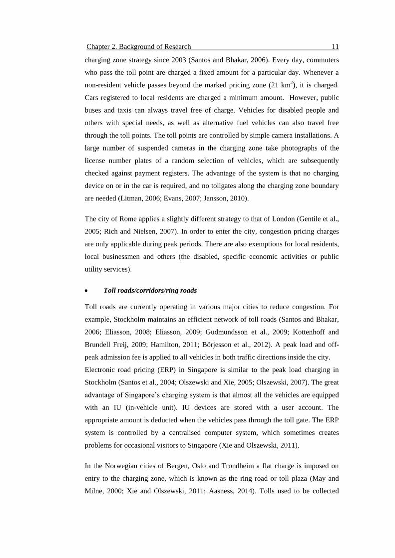
Figure 2.2: Classification of Modal Congestion Management Strategies.
Space Priority
Space priority or separate bus/tram lanes is a frequently used alternative to increase
public transport priority and reduce congestion. In busy urban areas, bus services
Modal congestion management
Time priority Space priority
Chapter 2. Background of Research 13
always face challenges due to traffic congestion. Many studies have revealed that the
preference for public transportation, such as bus or tram priority, provides shorter
average travel time and equal reliability for public transport compared to private
transport (Van Vugt et al. 1996). However, compared with train and light rail the
operation of buses is more likely to suffer from a range of effects including traffic
congestion (Lin et al. 2008). A number of studies have been done to develop bus
priority methodologies (Hounsell et al., 2008; Chen et al. 2008; Gough and Cook,
2010).
The study of Sterman and Schofer (1976) is one of the early studies on bus service
reliability in the United States. This study was conducted to test a particular measure
of reliability, the inverse of the standard deviation of point-to-point travel times, using
data from bus services in the Chicago area. Turnquist (1978) proposed a model for
estimating bus and passenger arrivals at a bus stop. The impacts on the expected
waiting time of the service frequency and reliability for random and non-random
arriving passengers were identified. Abkowitz and Engelstein (1983) studied factors
affecting the running time on transit routes and methods for maintaining transit service
regularity. These studies reported on estimating empirical models of transit mean
running time and identifying operations-control actions to improve reliability. It was
found that mean running time is strongly influenced by trip distance, people boarding
and alighting, and signalized intersections. The proposed method for maintaining
service regularity through improved scheduling and real-time control was found to be
a reasonable solution. Strathman and Hopper (1993) presented an empirical
assessment of factors affecting the on-time performance of the fixed route bus system
in Portland, Oregon. A multinomial model relating early, late, and on-time bus arrivals
to route, schedule, driver, and operating characteristics was developed and tested. The
model results showed that the probability of on-time failures increased during peak
periods, with longer headways and higher levels of passenger activity and as buses
progressed further along their routes. Yin et al. (2004) developed a generic simulation-
based approach to assess transit service reliability, taking into account the interaction
between the network performance and passengers’ route choice behaviour.
A high-capacity bus priority system has been installed in Sao Paulo as a solution to the
need for a low-cost urban transport solution (Tyler, 1991). The solution became
sufficiently successful that it has been tried and suggested in many developed
countries. This bus priority system in Sao Paulo operates on two slightly different
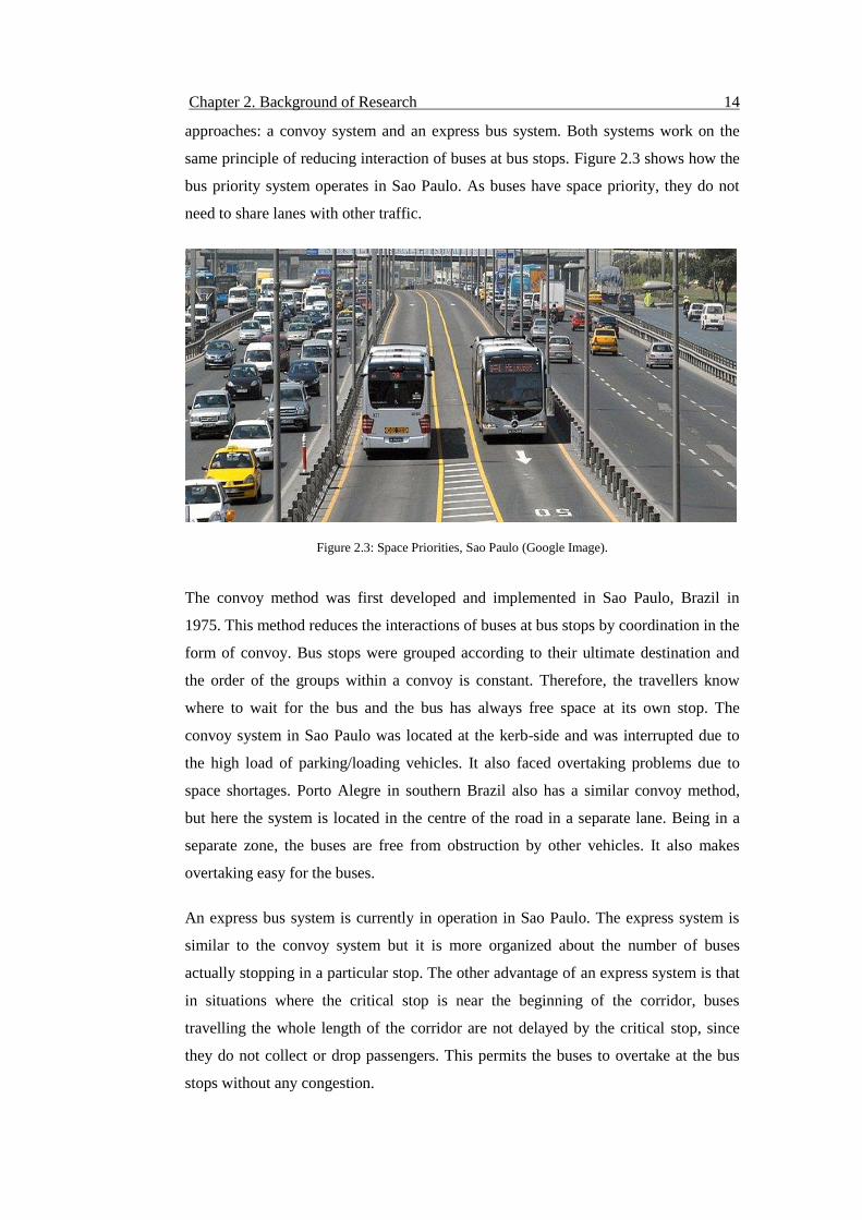
Chapter 2. Background of Research 14
approaches: a convoy system and an express bus system. Both systems work on the
same principle of reducing interaction of buses at bus stops. Figure 2.3 shows how the
bus priority system operates in Sao Paulo. As buses have space priority, they do not
need to share lanes with other traffic.
Figure 2.3: Space Priorities, Sao Paulo (Google Image).
The convoy method was first developed and implemented in Sao Paulo, Brazil in
1975. This method reduces the interactions of buses at bus stops by coordination in the
form of convoy. Bus stops were grouped according to their ultimate destination and
the order of the groups within a convoy is constant. Therefore, the travellers know
where to wait for the bus and the bus has always free space at its own stop. The
convoy system in Sao Paulo was located at the kerb-side and was interrupted due to
the high load of parking/loading vehicles. It also faced overtaking problems due to
space shortages. Porto Alegre in southern Brazil also has a similar convoy method,
but here the system is located in the centre of the road in a separate lane. Being in a
separate zone, the buses are free from obstruction by other vehicles. It also makes
overtaking easy for the buses.
An express bus system is currently in operation in Sao Paulo. The express system is
similar to the convoy system but it is more organized about the number of buses
actually stopping in a particular stop. The other advantage of an express system is that
in situations where the critical stop is near the beginning of the corridor, buses
travelling the whole length of the corridor are not delayed by the critical stop, since
they do not collect or drop passengers. This permits the buses to overtake at the bus
stops without any congestion.

Chapter 2. Background of Research 15
In cases with heavier traffic, even if dynamic locations of buses are exactly known,
when no dedicated bus lanes are provided, buses may still be involved in the general
traffic flow, sometimes having to suffer heavy time losses. In practice, because it is
not always possible to easily find free space for the bus lanes, especially in city
centres, permanent dedication of one lane in cases with lower frequencies of bus
services is very inefficient. This has led to the new concept of intermittent bus lanes
(IBLs) (Viegas and Lu, 2004). These are lanes in which the status of a given section
changes according to the presence or not of a bus in its spatial domain: when a bus is
approaching such a section, the status of that lane is changed to BUS lane, and after
the bus moves out of the section, it becomes a normal lane again, open to general
traffic. This ensures that the privileged lane status is active only for the time strictly
needed for the bus to operate with less delay, and the normal traffic does not suffer
much. The change of lane status is marked by the change of condition (on/off) of a
series of longitudinal lights along the line separating that lane from the next lane
(Viegas and Lu, 2004). Figure 2.4 represents a structure for IBL. The lane a1, 11(j)
marked in light green indicates the bus lane. The yellow circles indicate detectors
which detect the vehicles entering the lane.
Figure 2.4: Simplified Structure of IBL (Viegas and Lu 2004).
Transit lanes or (High Occupancy Vehicle (HOV) lanes are also a proven effective
solution to reduce congestion by modal management (Mesbah et al., 2011). HOV
lanes are currently in operation in different states of the USA, including Texas and
California (Kwon and Varaiya, 2008). The operation of HOV lanes varies depending
on the situation. Only vehicles carrying a certain number of passengers or HOVs can
use the transit lanes.
Chapter 2. Background of Research 16
Time Priority
Many studies have been devoted to develop time priority strategies. The conventional
fixed time signal control methods are based on historic data and are not very effective
for transit vehicles such as buses or trams (Yagar and Han, 1994). When a vehicle is
detected by a detector, two messages are recorded: (a) the vehicle type, i.e., whether it
is a private vehicle or public transit vehicle; (b) the detection time, i.e., the time at
which that vehicle is detected. The vehicle type is used to identify transit vehicles, so
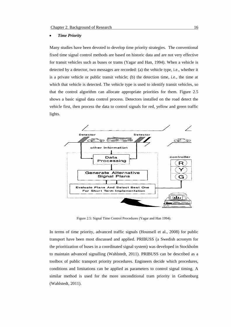
that the control algorithm can allocate appropriate priorities for them. Figure 2.5
shows a basic signal data control process. Detectors installed on the road detect the
vehicle first, then process the data to control signals for red, yellow and green traffic
lights.
Figure 2.5: Signal Time Control Procedures (Yagar and Han 1994).
In terms of time priority, advanced traffic signals (Hounsell et al., 2008) for public
transport have been most discussed and applied. PRIBUSS (a Swedish acronym for
the prioritization of buses in a coordinated signal system) was developed in Stockholm
to maintain advanced signalling (Wahlstedt, 2011). PRIBUSS can be described as a
toolbox of public transport priority procedures. Engineers decide which procedures,
conditions and limitations can be applied as parameters to control signal timing. A
similar method is used for the more unconditional tram priority in Gothenburg
(Wahlstedt, 2011).
Chapter 2. Background of Research 17
Advance signalling with Automatic Vehicle Location (AVL) is also one of the
solutions proposed (Chang et al., 1996) to reduce delay. Another signal or time
priority has been proposed by Yagar and Han (1994), called passive and active signal
timing. Passive signal timings can be set favouring approaches of trams/buses and
based on their fixed timetable. The time priority results in better congestion
management when the bus/tram has more frequency. Active signal priority triggers
priority measures when the vehicle is present. The vehicle is detected by the detectors
which send signals to the traffic signalling system for green extension or red
truncation. Active signal priority can be applied for buses/trams on a selected
intersection so that intersection delay can be minimised. It can also be arranged by
setting limits for extension lengths, by restricting the priority to uncongested time
periods and only giving priority too late or not to early trams/buses. In general, it is
difficult to analytically calculate the effects of dynamic signal timing or public
transport signal priority.
London has procured a modern AVL system for bus fleet management, passenger
information and bus priority. The new system is known as iBUS and is based on a
Global Positioning System (GPS) and supporting technology for bus location. The
system eliminates the need for on-street hardware for detecting buses and provides
more flexibility and opportunity for using bus detectors (Hounsell et al., 2008).
2.3 Limitations of Existing Studies
The literature regarding the modal management strategies covers a wide range
of theories based on mathematical algorithms and survey results.
Very few case studies of solving congestion problems using software analysis
of a whole network or a single intersection are available.
Some ideas have been developed to control congestion for both tram and bus
priority without hampering other traffic. However, the application of modal
management strategies to a particular intersection in Melbourne with different
modes of transport including tram or light rail, bus, private car and pedestrians
is absent.
For tram priority, Melbourne uses separate tram lanes for different routes but
they are not provided with signal priority.
Chapter 2. Background of Research 18
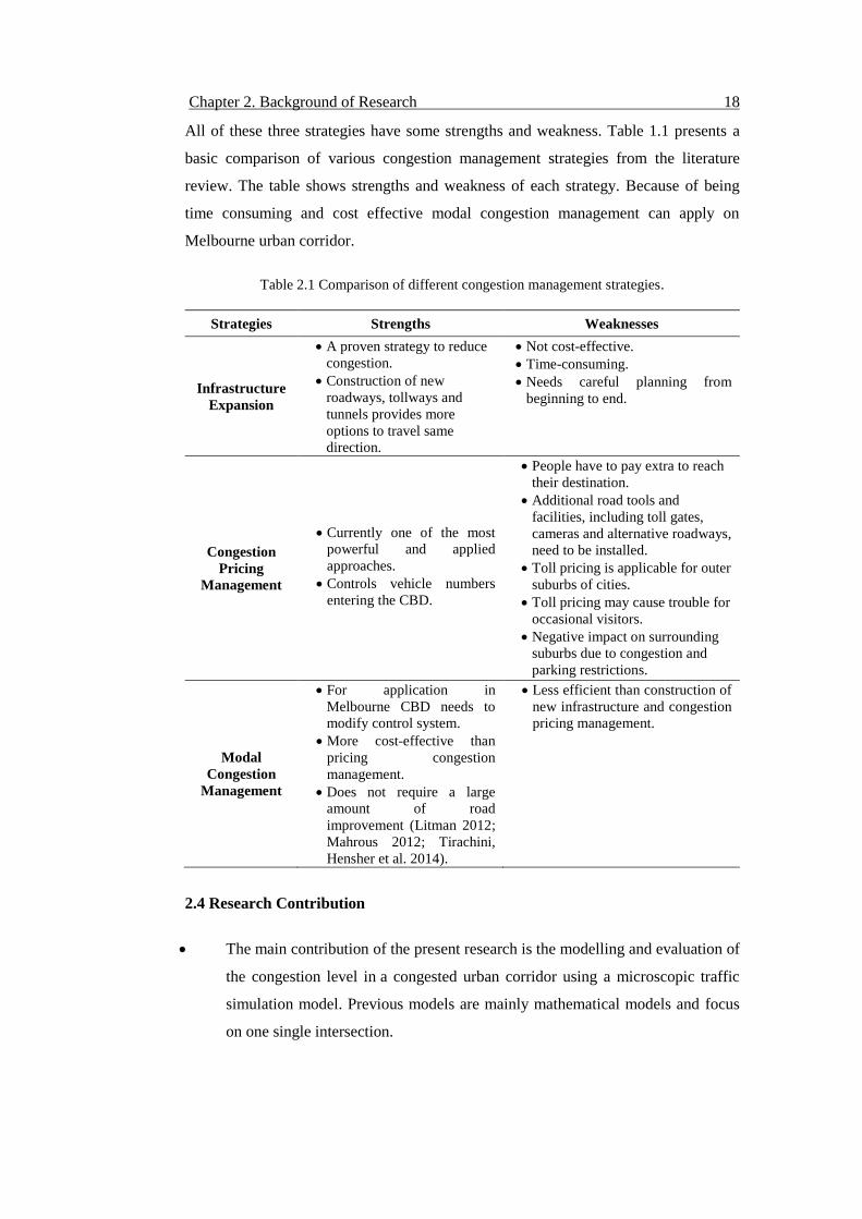
All of these three strategies have some strengths and weakness. Table 1.1 presents a
basic comparison of various congestion management strategies from the literature
review. The table shows strengths and weakness of each strategy. Because of being
time consuming and cost effective modal congestion management can apply on
Melbourne urban corridor.
Table 2.1 Comparison of different congestion management strategies.
Strategies Strengths Weaknesses
Infrastructure
Expansion
A proven strategy to reduce
congestion.
Construction of new
roadways, tollways and
tunnels provides more
options to travel same
direction.
Not cost-effective.
Time-consuming.
Needs careful planning from
beginning to end.
Congestion
Pricing
Management
Currently one of the most
powerful and applied
approaches.
Controls vehicle numbers
entering the CBD.
People have to pay extra to reach
their destination.
Additional road tools and
facilities, including toll gates,
cameras and alternative roadways,
need to be installed.
Toll pricing is applicable for outer
suburbs of cities.
Toll pricing may cause trouble for
occasional visitors.
Negative impact on surrounding
suburbs due to congestion and
parking restrictions.
Modal
Congestion
Management
For application in
Melbourne CBD needs to
modify control system.
More cost-effective than
pricing congestion
management.
Does not require a large
amount of road
improvement (Litman 2012;
Mahrous 2012; Tirachini,
Hensher et al. 2014).
Less efficient than construction of
new infrastructure and congestion
pricing management.
2.4 Research Contribution
The main contribution of the present research is the modelling and evaluation of
the congestion level in a congested urban corridor using a microscopic traffic
simulation model. Previous models are mainly mathematical models and focus
on one single intersection.
Chapter 2. Background of Research 19
Another contribution is the use of multi-modal strategies to control all existing
modes of transport, including passenger cars, buses, trams and cyclists.
The study focuses on modal congestion management as it is a more economical
solution than the construction of new infrastructure and congestion pricing strategies.
The research will contribute specific knowledge and strategies for a congested
corridor in Melbourne.
This research will provide specific knowledge of strategies for modal congestion
management. The study will propose better strategies to reduce traffic congestion for a
corridor with pedestrians and different modes of transport, including trams, buses,
passenger cars and bicycles using the SIDRA 6 software.
2.5 Summary
This chapter has provided a review of the existing methods of control congestion and
explained their strengths and weaknesses. On the basis of previous studies, modal
congestion management is most suitable for the Melbourne CBD as it is less
expensive than the other two methods. This study applies strategies to a case study
approach and proposes better strategies to reduce congestion for the morning peak
period.
20
Chapter 3
Research Framework
3.1 Introduction
The primary purpose of this research is to apply modal congestion management
strategies to reduce traffic congestion. The improved approaches will be presented
based on a review of the literature and an evaluation of the strategies. The methods
applied will be influenced by traffic characteristics, with a focus of traffic volume,
geometric information, average speed, travel times, delay at intersections and signal
timing. This chapter discusses the methods used in this study, the case study corridor
selected and the range and types of data collected.
3.2 Study Corridor
The site selected for this research is a corridor from Melbourne near Kew. The
corridor starts from the Manningtree Road and Power Street intersection in Hawthorn
to the intersection of Princes Street and Beatrice Street in Kew (M21, Melways Ref:
page 45, C11; Date 15th July, 2014).
The corridor is about 2.1 km long. Each direction of the corridor has various lanes.
The daily traffic volume of the corridor is (annual average) 7, 91, 013 nos per day.
The intersection of Princess Street, Studley Street, High Street South, Denmark Street
and High Street is one of the busiest and congested intersections in Melbourne. Tram,
Bus, Motor vehicles, Bi-cycle and Pedestrian operates through this intersection. Off-
street parking lanes also provided on different approaches. Dedicated lane and signals
provided for bus and tram throughout the intersection.
Chapter 2. Background of Research 21
3.2.1. Area of Study
The corridor includes fifteen different intersections as follows:
Intersections of Princess Street, Studley Street, High Street South, Denmark
Street and High Street.
Intersection of Wellington Street and Denmark Street.
Intersection of Stevenson Street and Denmark Street.
Intersection of Barker Road, Power Street and Denmark Street.
Most of the intersections are T-intersections. Four major congested intersections have
been selected, according to VicRoads data to configure this corridor. The research
simulates these four intersections separately as well as in a network to observe the
effects. Figure 3.1 shows the Google map of the case study corridor. Points A and B
indicate the start and end points.
Figure 3.1: Google map for the case study corridor.
Chapter 3. Research Framework 22
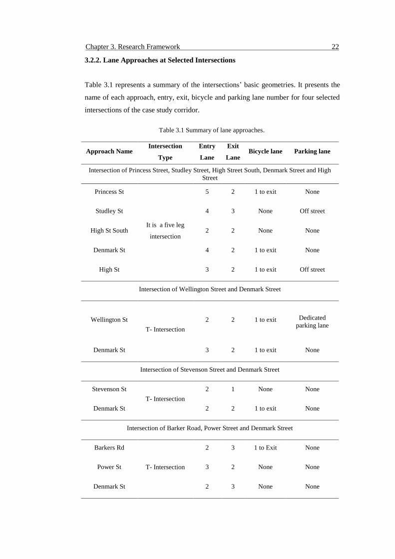
3.2.2. Lane Approaches at Selected Intersections
Table 3.1 represents a summary of the intersections’ basic geometries. It presents the
name of each approach, entry, exit, bicycle and parking lane number for four selected
intersections of the case study corridor.
Table 3.1 Summary of lane approaches.
Approach Name Intersection
Type
Entry
Lane
Exit
Lane Bicycle lane Parking lane
Intersection of Princess Street, Studley Street, High Street South, Denmark Street and High
Street
Princess St
It is a five leg
intersection
5 2 1 to exit None
Studley St 4 3 None Off street
High St South 2 2 None None
Denmark St 4 2 1 to exit None
High St 3 2 1 to exit Off street
Intersection of Wellington Street and Denmark Street
Wellington St
T- Intersection
2 2 1 to exit Dedicated
parking lane
Denmark St 3 2 1 to exit None
Intersection of Stevenson Street and Denmark Street
Stevenson St
T- Intersection
2 1 None None
Denmark St 2 2 1 to exit None
Intersection of Barker Road, Power Street and Denmark Street
Barkers Rd
T- Intersection
2 3 1 to Exit None
Power St 3 2 None None
Denmark St 2 3 None None
Chapter 3. Research Framework 23
3.3 Methodology
The study aim is to propose efficient strategies to control congestion for a selected
corridor using SIDRA analysis. Strategies are applied to different modes of transport
to control congestion. Travel speed, queue distance and average delay are the main
three parameters compared. The steps were as follows:
Modelling of the corridor in SIDRA
The traffic conditions on four intersections with same number of lanes, traffic
volumes, bus/tram frequencies and signal cycle times are simulated. The
simulation data are collected from VicRoads, surveys, Yarra Trams system
information, bus system information and Google maps. In the case of any
differences of actual network conditions and the SIDRA simulated intersection
model, input parameters are calibrated. If the observed intersection condition
and SIDRA simulated intersection model are similar, the SIDRA model is
identified as validated. Therefore, all the intersections are added according to
the case study corridor and simulated as a network in SIDRA. The simulated
SIDRA network model needs to be calibrated and validated with actual corridor
conditions.
Identification of different strategies
Different modal congestion management strategies to reduce traffic congestion
are identified. Space priority for trams/buses at intersection/corridor is one of
the proposed and applied strategies in different cities. Modifying signal time (i.e
extended green or early green signal) during peak periods of the day is another
proposed strategy to control traffic congestion. Parking restrictions and removal
of bicycle lanes are also utilized to reduce congestion around different
intersections.
Simulation of different strategies
The research simulates different identified strategies to determine the effect on
intersections and the corridor/network. The study applies each strategy on each
Chapter 3. Research Framework 24
intersection to see the effect of congestion. Based on the results, the best
methods from intersection models are selected and apply to the whole
network/corridor.
Comparison of applied strategies
The study compares simulated models of the network/corridor with present
conditions and proposes better methods to control congestion. Three main
parameters are used to compare strategies. The variables used for comparison
are travel speed, queue length and average delay.
3.4 Datasets
Datasets are collected from VicRoads SCATS data, surveys, Google maps and Yarra
Trams/bus system information. Using these data the case study corridor is modelled
first. After modelling the corridor will be validated with actual collected data.
3.4.1 VicRoads SCATS Data
VicRoads was the main source of data for this project. In Melbourne, the SCATS
(Sydney Coordinated Adaptive Traffic System) are used for traffic control. SCATS
primarily manages the dynamic (on-line, real-time) timing of signal phases at traffic
signals, meaning that it tries to find the best phasing (i.e. cycle times, phase splits and
offsets) for the current traffic situation for individual intersections as well as for the
whole network. The SCATS system uses sensors at each traffic signal to detect vehicle
presence in each lane and pedestrians waiting to cross at the local site. The vehicle
sensors are generally inductive loops installed within the road pavement. The
pedestrian sensors are usually push buttons. Various other types of sensors can be used
for vehicle presence detection, provided that similar and consistent output is achieved.
Information collected from the vehicle sensors allows SCATS to calculate and adapt
the timing of traffic signals in the network. From the SCATS system VicRoads
provides the following data sets:
Chapter 3. Research Framework 25
Intersection Grouping: VicRoads named the intersection to different groups.
For the same group of sites signal phase settings and signal cycle timing are
similar.
Controller Time Setting & Phasing Diagram: Signal phase length for each
intersection, total time for green, red, yellow, maximum green and extension of
green signal time for both vehicle and pedestrian are described. The signal
phase diagrams present the order of traffic signals, priority for any transport
mode and extension signal upon demand.
Detector Details: The data sets provide contained information about detector
type and location. The SCATS datasets provide information about numbers of
detectors located at intersections, types of detectors (i.e, vehicle detectors,
pedestrian push-button detectors, bicycle push-button detectors, radio-
controlled vehicle detectors and video detectors). The datasets also provide
particulars of vehicle movement direction detected by assigned detectors.
Traffic Volume: The data set covers total traffic volume from May, 2012 to
May, 2013. VicRoads also provided more recent data from 10th February, 2014
to 16th February, 2014. Traffic volume data were calculated from detectors for
24 hours at 15 minute intervals.
3.4.2 Surveys
Data sets collected from field surveys of the corridor as follows:
Intersection geometric details: Geometric measurements of all the
intersections i.e, number of lanes, lane length, lane width, number of
approaches per intersection for both vehicle and cycle lanes is collected.
Movement: Details of movement of vehicles from one direction to
straight/left/right direction, movement restriction for any selected direction
during peak/off peak time and proportion of vehicles turning left/right at all the
intersections are collected during Surveys.
Chapter 3. Research Framework 26
Speed & Average Speed: Speed limits for different approaches are noted for
morning peak time. During the morning peak period the speed limit is variable.
The average speed for different approaches, travel time and back of queue
length are measured for validation of the corridor model.
Back of queue & Gap acceptance: Back of queue is observed all the
congested approaches. The intersection was surveyed for the AM peak period. It
is difficult to ascertain exactly what the average gap acceptance for drivers at
the intersections. The accepted gap time is observed greater during the right or
left turn than straight moving vehicle.
3.4.3 Google Maps
Intersection measurement: Distance from one intersection to next intersection
and back of queue length is calculated.
3.4.4 Yarra Trams/Bus System Information
Tram timetables and numbers: Tram operation times, frequencies and
number of trams operating along the corridor during peak periods.
3.5 Summary of Various Datasets
Datasets are collected for one morning peak hour (7.30 am to 8.30 am) from various
sources. Traffic volume from 11th February, 2014 is used for this simulation and
calibration. Table 3.2 shows a summary of intersections by VicRoads. VicRoads gives
each intersection a number to make identification easy.
Table 3.2 Summary of Intersection Grouping.*
Intersection Name Site
Grouping
Princess Street/Studley Street/High Street South/ Denmark Street/ High Street 3662
Denmark Street/Wellington Street 3663
Denmark Street /Stevenson Street 1190
Denmark Street/Power Street/Barkers Road 3002
* VicRoads SCATS Data.
Chapter 3. Research Framework 27
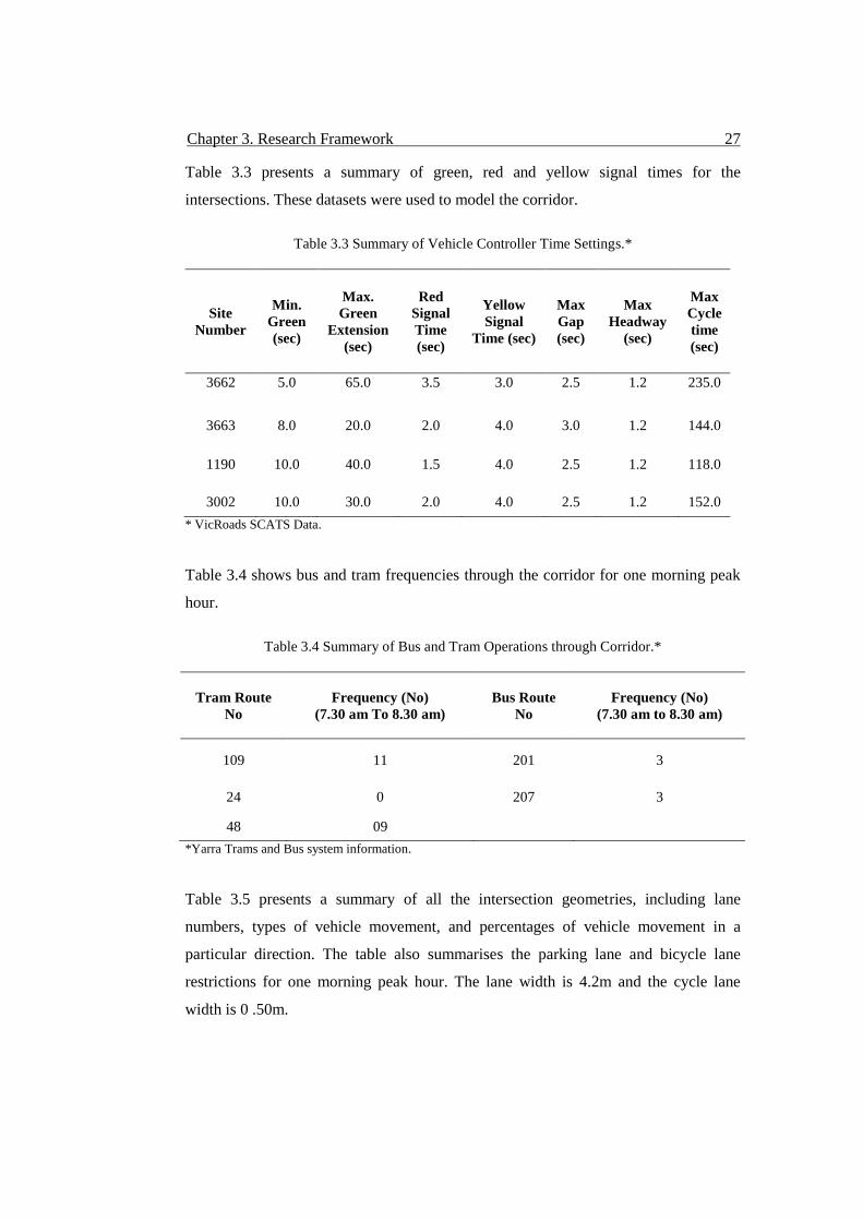
Table 3.3 presents a summary of green, red and yellow signal times for the
intersections. These datasets were used to model the corridor.
Table 3.3 Summary of Vehicle Controller Time Settings.*
Site
Number
Min.
Green
(sec)
Max.
Green
Extension
(sec)
Red
Signal
Time
(sec)
Yellow
Signal
Time (sec)
Max
Gap
(sec)
Max
Headway
(sec)
Max
Cycle
time
(sec)
3662 5.0 65.0 3.5 3.0 2.5 1.2 235.0
3663 8.0 20.0 2.0 4.0 3.0 1.2 144.0
1190 10.0 40.0 1.5 4.0 2.5 1.2 118.0
3002 10.0 30.0 2.0 4.0 2.5 1.2 152.0
* VicRoads SCATS Data.
Table 3.4 shows bus and tram frequencies through the corridor for one morning peak
hour.
Table 3.4 Summary of Bus and Tram Operations through Corridor.*
Tram Route
No
Frequency (No)
(7.30 am To 8.30 am)
Bus Route
No
Frequency (No)
(7.30 am to 8.30 am)
109 11 201 3
24 0 207 3
48 09
*Yarra Trams and Bus system information.
Table 3.5 presents a summary of all the intersection geometries, including lane
numbers, types of vehicle movement, and percentages of vehicle movement in a
particular direction. The table also summarises the parking lane and bicycle lane
restrictions for one morning peak hour. The lane width is 4.2m and the cycle lane
width is 0 .50m.
Chapter 3. Research Framework 28
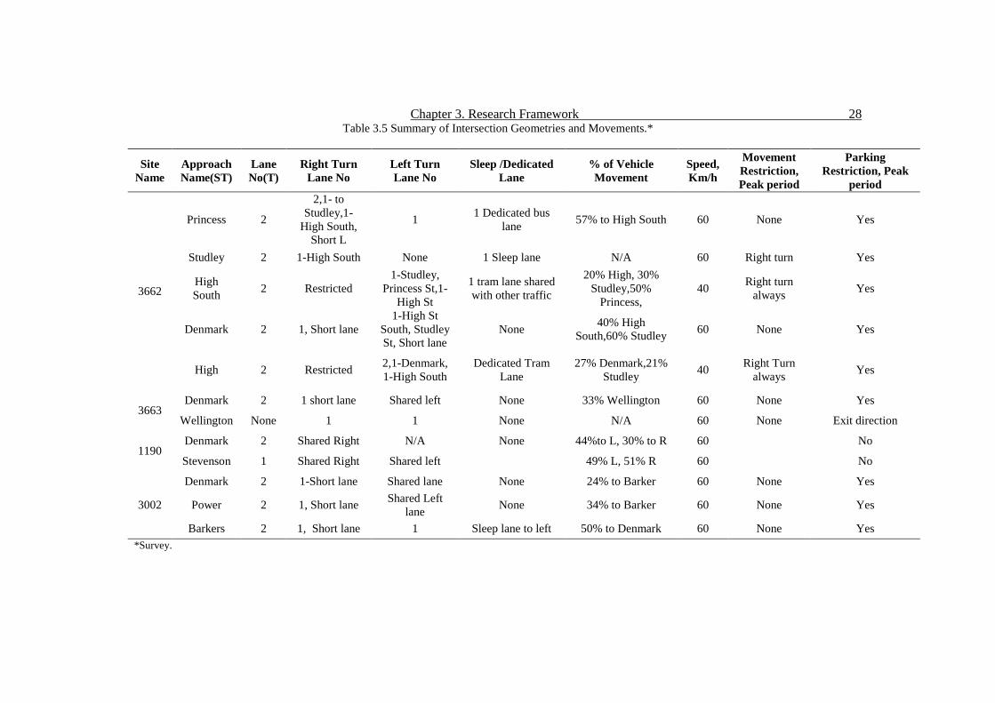
Table 3.5 Summary of Intersection Geometries and Movements.*
Site
Name
Approach
Name(ST)
Lane
No(T)
Right Turn
Lane No
Left Turn
Lane No
Sleep /Dedicated
Lane
% of Vehicle
Movement
Speed,
Km/h
Movement
Restriction,
Peak period
Parking
Restriction, Peak
period
3662
Princess 2
2,1- to
Studley,1-
High South,
Short L
1 1 Dedicated bus
lane 57% to High South 60 None Yes
Studley 2 1-High South None 1 Sleep lane N/A 60 Right turn Yes
High
South 2 Restricted
1-Studley,
Princess St,1-
High St
1 tram lane shared
with other traffic
20% High, 30%
Studley,50%
Princess,
40 Right turn
always Yes
Denmark 2 1, Short lane
1-High St
South, Studley
St, Short lane
None 40% High
South,60% Studley 60 None Yes
High 2 Restricted 2,1-Denmark,
1-High South
Dedicated Tram
Lane
27% Denmark,21%
Studley 40
Right Turn
always Yes
3663 Denmark 2 1 short lane Shared left None 33% Wellington 60 None Yes
Wellington None 1 1 None N/A 60 None Exit direction
1190 Denmark 2 Shared Right N/A None 44%to L, 30% to R 60 No
Stevenson 1 Shared Right Shared left 49% L, 51% R 60 No
3002
Denmark 2 1-Short lane Shared lane None 24% to Barker 60 None Yes
Power 2 1, Short lane Shared Left
lane None 34% to Barker 60 None Yes
Barkers 2 1, Short lane 1 Sleep lane to left 50% to Denmark 60 None Yes
*Survey.

Chapter 3. Research Framework 29
3.6 Summary
This chapter has discussed the research methodology and presents details of the
datasets collected for model simulation and validation. The datasets are used to
calibrate different input parameters for intersection/corridor modelling. Therefore, this
chapter has provided information about the types of input parameter values used in the
software.
30
Chapter 4
Model Development
4.1 Introduction
Chapter 3 discussed the data sets for corridor modelling and the methodology of the
present research. This chapter provides a brief outline of the micro analytical software
SIDRA (SIDRA 2013). The chapter also explains the step-by-step procedures in
modelling the corridor using different parameters and the validation procedures for
each intersection and the corridor.
4.2 SIDRA Intersection
The Signalised (and un-signalised) Intersection Design and Research Aid (SIDRA)
(SIDRA 2013) software is an advanced lane-based micro-analytical tool for the design
and evaluation of individual intersections and networks of intersections, including the
modelling of separate movement classes (light vehicles, heavy vehicles, buses,
bicycles, large trucks, light rail/trams and so on). It provides estimates of capacity and
levels of service and a wide range of performance measures, including delay, queue
length and stops for vehicles and pedestrians, as well as fuel consumption, pollutant
emissions and operating costs (SIDRA, 2013). For the present research the latest
version 6 is used. SIDRA Intersection 6 has a number of input and output parameters
to model and validate. SIDRA can join various intersections to a corridor/network and
analyse the effects. The output results can form individual approaches, intersections
and networks. SIDRA standard model, HCM model and TWSC calibration parameter
are used for modelling, calibration and validation.
4.3 Corridor Modelling
To configure the corridor each intersection must be modelled separately according to
the datasets (Akcelik, 1997; Akcelik, 2012). Therefore it is necessary to model,
Chapter 4. Model Development 31
calibrate and validate according to the datasets collected. Output results are produced
in table and layout formats. Output results can be measured for any parameter by
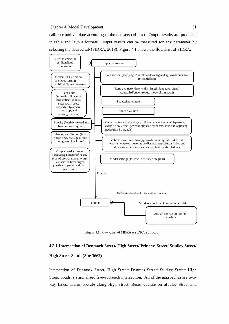
selecting the desired tab (SIDRA, 2013). Figure 4.1 shows the flowchart of SIDRA.
Figure 4.1: Flow chart of SIDRA ((SIDRA Software).
4.3.1 Intersection of Denmark Street/ High Street/ Princess Street/ Studley Street/
High Street South (Site 3662)
Intersection of Denmark Street/ High Street/ Princess Street/ Studley Street/ High
Street South is a signalised five-approach intersection. All of the approaches are two-
way lanes. Trams operate along High Street. Buses operate on Studley Street and
Select Intersection
as Signalised
Intersection Input parameters
Intersection type (single/two /three/four leg and approach distance
for modelling)
Lane geometry (lane width, length, lane type, signal
controlled/uncontrolled, mode of transport)
Pedestrian volume
Traffic volume
Movement Definition (vehicles turning
right/left/through/u-turn)
Lane Data (saturation flow rate,
lane utilization ratio,
saturation speed,
capacity adjustment,
bus stop, and
blockage of lane)
Priority (Vehicle toward any
direction moving first)
Gap acceptance (critical gap, follow-up headway, end departure, exiting flow effect, per cent opposed by nearest lane and opposing
pedestrian by signals)
Output results format (analysing number of years,
type of growth model, worst
lane service level target, practical capacity and final
year result)
Model settings (for level of service diagram)
Phasing and Timing (total
phase time, red signal time
and green signal time) Vehicle movement data (approach cruise speed, exit speed,
negotiation speed, negotiation distance, negotiation radius and
downstream distance values required for simulation.)
Process
Output
Calibrate simulated intersection models
Validate simulated intersection models
Add all intersection to form
corridor
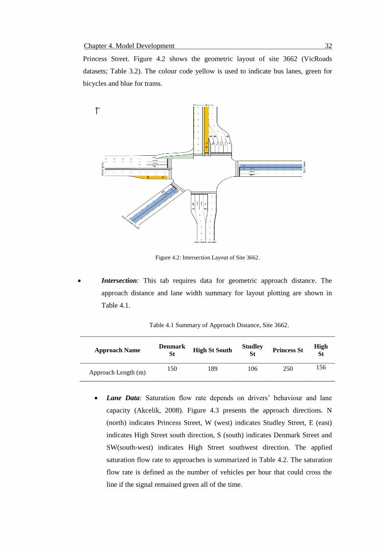
Chapter 4. Model Development 32
Princess Street. Figure 4.2 shows the geometric layout of site 3662 (VicRoads
datasets; Table 3.2). The colour code yellow is used to indicate bus lanes, green for
bicycles and blue for trams.
Figure 4.2: Intersection Layout of Site 3662.
Intersection: This tab requires data for geometric approach distance. The
approach distance and lane width summary for layout plotting are shown in
Table 4.1.
Table 4.1 Summary of Approach Distance, Site 3662.
Approach Name Denmark
St High St South
Studley
St Princess St
High
St
Approach Length (m) 150 189 106 250 156
Lane Data: Saturation flow rate depends on drivers’ behaviour and lane
capacity (Akcelik, 2008). Figure 4.3 presents the approach directions. N
(north) indicates Princess Street, W (west) indicates Studley Street, E (east)
indicates High Street south direction, S (south) indicates Denmark Street and
SW(south-west) indicates High Street southwest direction. The applied
saturation flow rate to approaches is summarized in Table 4.2. The saturation
flow rate is defined as the number of vehicles per hour that could cross the
line if the signal remained green all of the time.
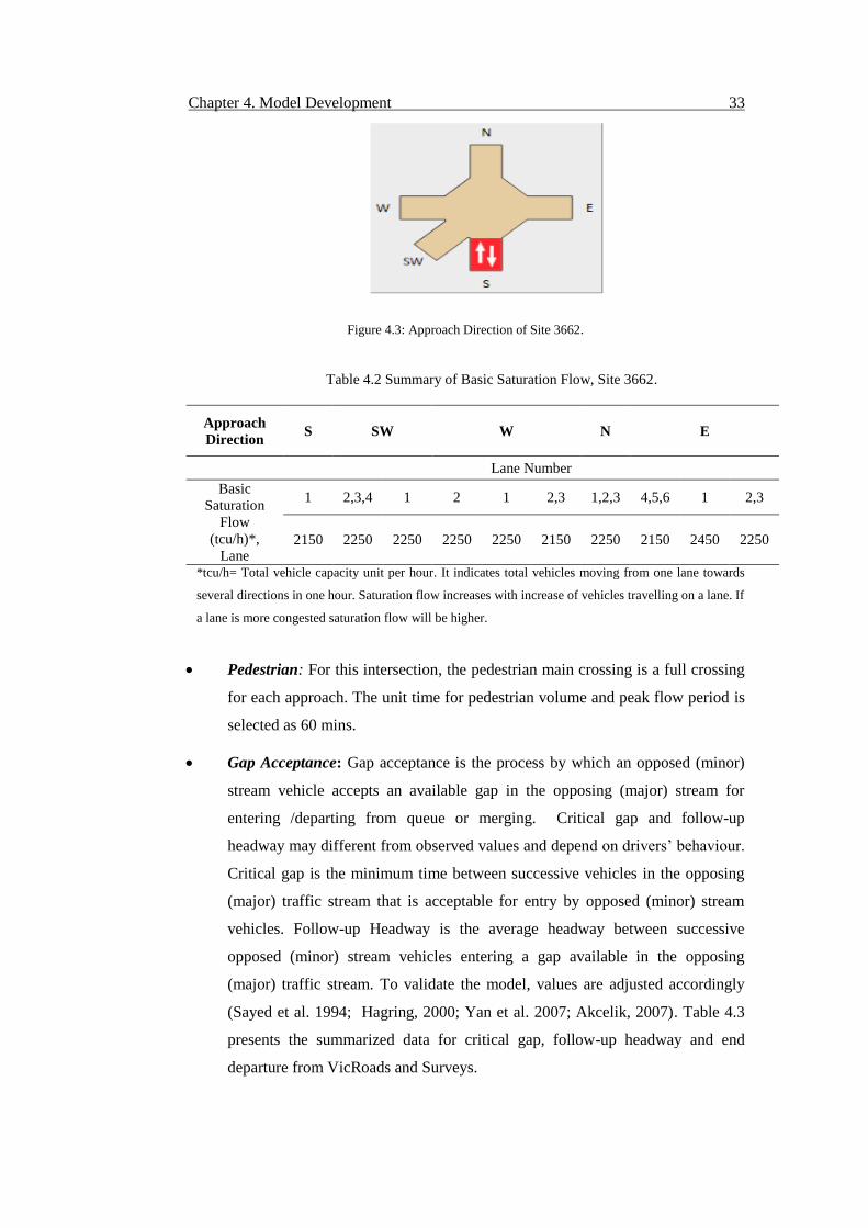
Chapter 4. Model Development 33
Figure 4.3: Approach Direction of Site 3662.
Table 4.2 Summary of Basic Saturation Flow, Site 3662.
Approach
Direction S SW W N E
Lane Number
Basic
Saturation
Flow
(tcu/h)*,
Lane
1 2,3,4 1 2 1 2,3 1,2,3 4,5,6 1 2,3
2150 2250 2250 2250 2250 2150 2250 2150 2450 2250
*tcu/h= Total vehicle capacity unit per hour. It indicates total vehicles moving from one lane towards
several directions in one hour. Saturation flow increases with increase of vehicles travelling on a lane. If
a lane is more congested saturation flow will be higher.
Pedestrian: For this intersection, the pedestrian main crossing is a full crossing
for each approach. The unit time for pedestrian volume and peak flow period is
selected as 60 mins.
Gap Acceptance: Gap acceptance is the process by which an opposed (minor)
stream vehicle accepts an available gap in the opposing (major) stream for
entering /departing from queue or merging. Critical gap and follow-up
headway may different from observed values and depend on drivers’ behaviour.
Critical gap is the minimum time between successive vehicles in the opposing
(major) traffic stream that is acceptable for entry by opposed (minor) stream
vehicles. Follow-up Headway is the average headway between successive
opposed (minor) stream vehicles entering a gap available in the opposing
(major) traffic stream. To validate the model, values are adjusted accordingly
(Sayed et al. 1994; Hagring, 2000; Yan et al. 2007; Akcelik, 2007). Table 4.3
presents the summarized data for critical gap, follow-up headway and end
departure from VicRoads and Surveys.
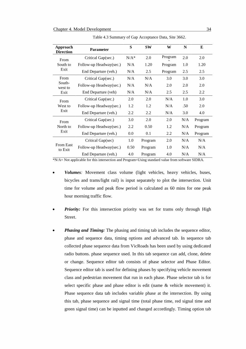
Chapter 4. Model Development 34
Table 4.3 Summary of Gap Acceptance Data, Site 3662.
Approach
Direction Parameter
S
SW
W
N
E
From
South to
Exit
Critical Gap(sec.) N/A* 2.0 Program
* 2.0 2.0
Follow-up Headway(sec.) N/A 1.20 Program 1.0 1.20
End Departure (veh.) N/A 2.5 Program 2.5 2.5
From
South-
west to
Exit
Critical Gap(sec.) N/A N/A 3.0 3.0 3.0
Follow-up Headway(sec.) N/A N/A 2.0 2.0 2.0
End Departure (veh) N/A N/A 2.5 2.5 2.2
From
West to
Exit
Critical Gap(sec.) 2.0 2.0 N/A 1.0 3.0
Follow-up Headway(sec.) 1.2 1.2 N/A .50 2.0
End Departure (veh.) 2.2 2.2 N/A 3.0 4.0
From
North to
Exit
Critical Gap(sec.) 3.0 2.0 2.0 N/A Program
Follow-up Headway(sec.) 2.2 0.50 1.2 N/A Program
End Departure (veh.) 0.0 0.1 2.2 N/A Program
From East
to Exit
Critical Gap(sec) 1.0 Program 2.0 N/A N/A
Follow-up Headway(sec.) 0.50 Program 1.0 N/A N/A
End Departure (veh.) 4.0 Program 4.0 N/A N/A
*N/A= Not applicable for this intersection and Program=Using standard value from software SIDRA.
Volumes: Movement class volume (light vehicles, heavy vehicles, buses,
bicycles and trams/light rail) is input separately to plot the intersection. Unit
time for volume and peak flow period is calculated as 60 mins for one peak
hour morning traffic flow.
Priority: For this intersection priority was set for trams only through High
Street.
Phasing and Timing: The phasing and timing tab includes the sequence editor,
phase and sequence data, timing options and advanced tab. In sequence tab
collected phase sequence data from VicRoads has been used by using dedicated
radio buttons. phase sequence used. In this tab sequence can add, clone, delete
or change. Sequence editor tab consists of phase selector and Phase Editor.
Sequence editor tab is used for defining phases by specifying vehicle movement
class and pedestrian movement that run in each phase. Phase selector tab is for
select specific phase and phase editor is edit (name & vehicle movement) it.
Phase sequence data tab includes variable phase at the intersection. By using
this tab, phase sequence and signal time (total phase time, red signal time and
green signal time) can be inputted and changed accordingly. Timing option tab
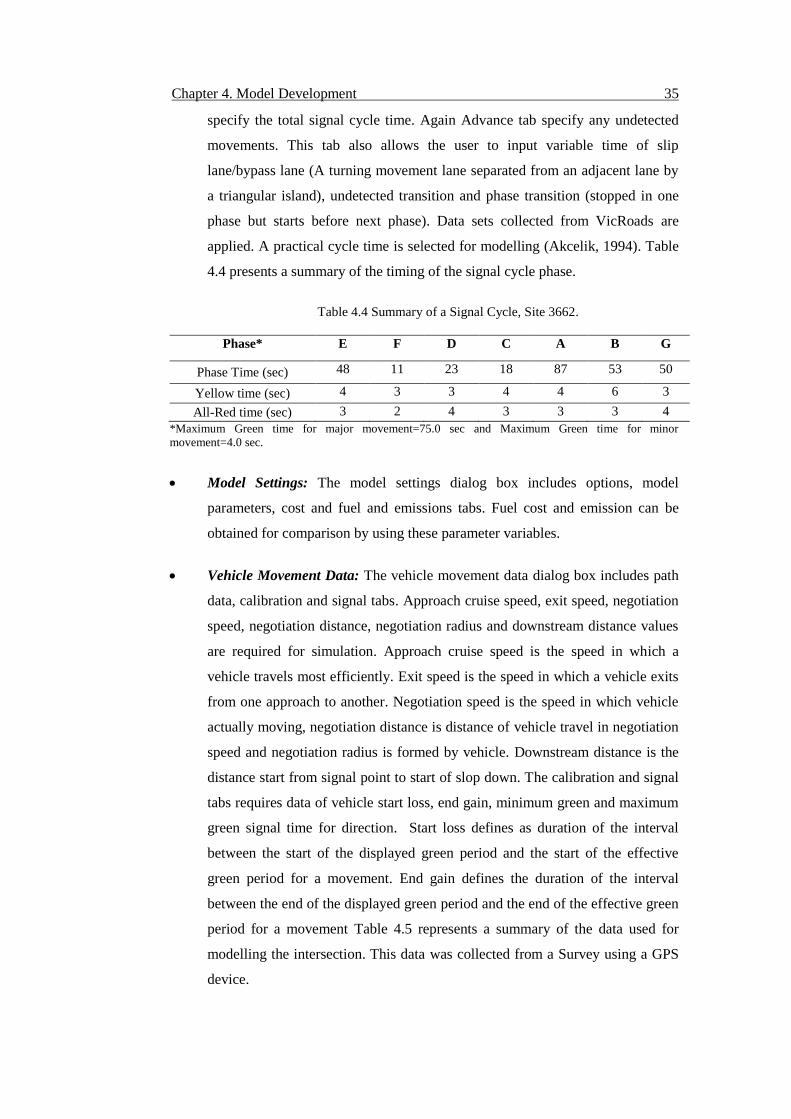
Chapter 4. Model Development 35
specify the total signal cycle time. Again Advance tab specify any undetected
movements. This tab also allows the user to input variable time of slip
lane/bypass lane (A turning movement lane separated from an adjacent lane by
a triangular island), undetected transition and phase transition (stopped in one
phase but starts before next phase). Data sets collected from VicRoads are
applied. A practical cycle time is selected for modelling (Akcelik, 1994). Table
4.4 presents a summary of the timing of the signal cycle phase.
Table 4.4 Summary of a Signal Cycle, Site 3662.
Phase* E F D C A B G
Phase Time (sec) 48 11 23 18 87 53 50
Yellow time (sec) 4 3 3 4 4 6 3
All-Red time (sec) 3 2 4 3 3 3 4
*Maximum Green time for major movement=75.0 sec and Maximum Green time for minor
movement=4.0 sec.
Model Settings: The model settings dialog box includes options, model
parameters, cost and fuel and emissions tabs. Fuel cost and emission can be
obtained for comparison by using these parameter variables.
Vehicle Movement Data: The vehicle movement data dialog box includes path
data, calibration and signal tabs. Approach cruise speed, exit speed, negotiation
speed, negotiation distance, negotiation radius and downstream distance values
are required for simulation. Approach cruise speed is the speed in which a
vehicle travels most efficiently. Exit speed is the speed in which a vehicle exits
from one approach to another. Negotiation speed is the speed in which vehicle
actually moving, negotiation distance is distance of vehicle travel in negotiation
speed and negotiation radius is formed by vehicle. Downstream distance is the
distance start from signal point to start of slop down. The calibration and signal
tabs requires data of vehicle start loss, end gain, minimum green and maximum
green signal time for direction. Start loss defines as duration of the interval
between the start of the displayed green period and the start of the effective
green period for a movement. End gain defines the duration of the interval
between the end of the displayed green period and the end of the effective green
period for a movement Table 4.5 represents a summary of the data used for
modelling the intersection. This data was collected from a Survey using a GPS
device.
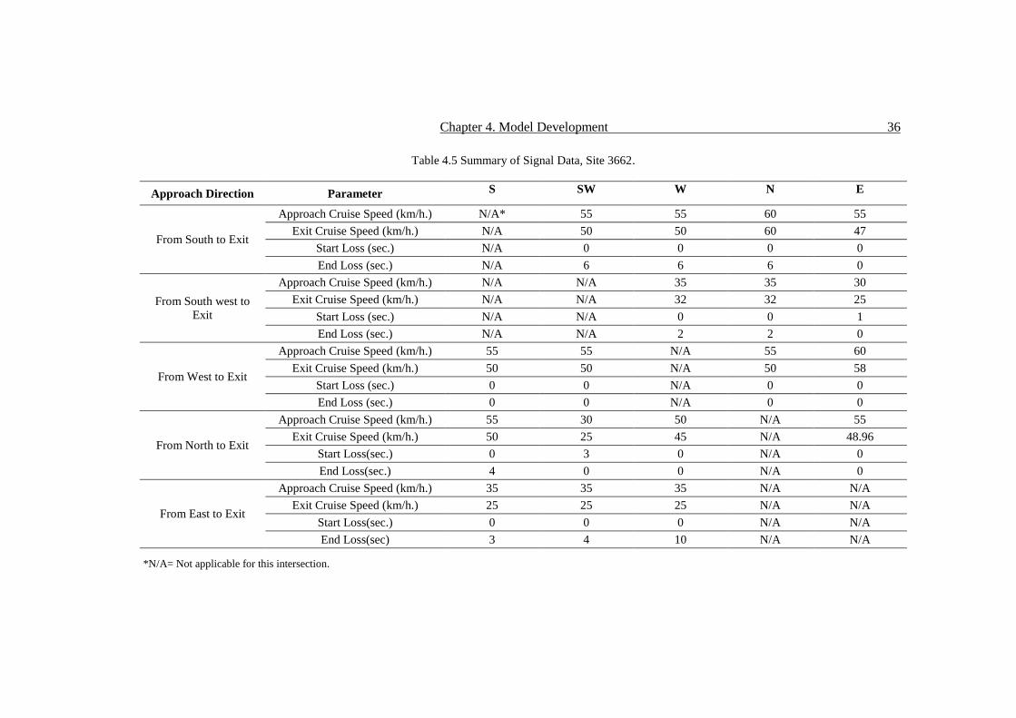
Chapter 4. Model Development 36
Table 4.5 Summary of Signal Data, Site 3662.
Approach Direction Parameter S
SW
W
N
E
From South to Exit
Approach Cruise Speed (km/h.) N/A* 55 55 60 55
Exit Cruise Speed (km/h.) N/A 50 50 60 47
Start Loss (sec.) N/A 0 0 0 0
End Loss (sec.) N/A 6 6 6 0
From South west to
Exit
Approach Cruise Speed (km/h.) N/A N/A 35 35 30
Exit Cruise Speed (km/h.) N/A N/A 32 32 25
Start Loss (sec.) N/A N/A 0 0 1
End Loss (sec.) N/A N/A 2 2 0
From West to Exit
Approach Cruise Speed (km/h.) 55 55 N/A 55 60
Exit Cruise Speed (km/h.) 50 50 N/A 50 58
Start Loss (sec.) 0 0 N/A 0 0
End Loss (sec.) 0 0 N/A 0 0
From North to Exit
Approach Cruise Speed (km/h.) 55 30 50 N/A 55
Exit Cruise Speed (km/h.) 50 25 45 N/A 48.96
Start Loss(sec.) 0 3 0 N/A 0
End Loss(sec.) 4 0 0 N/A 0
From East to Exit
Approach Cruise Speed (km/h.) 35 35 35 N/A N/A
Exit Cruise Speed (km/h.) 25 25 25 N/A N/A
Start Loss(sec.) 0 0 0 N/A N/A
End Loss(sec) 3 4 10 N/A N/A
*N/A= Not applicable for this intersection.
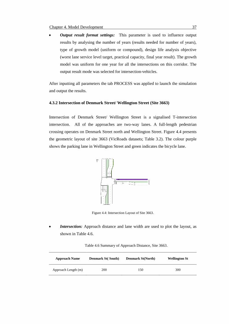
Chapter 4. Model Development 37
Output result format settings: This parameter is used to influence output
results by analysing the number of years (results needed for number of years),
type of growth model (uniform or compound), design life analysis objective
(worst lane service level target, practical capacity, final year result). The growth
model was uniform for one year for all the intersections on this corridor. The
output result mode was selected for intersection-vehicles.
After inputting all parameters the tab PROCESS was applied to launch the simulation
and output the results.
4.3.2 Intersection of Denmark Street/ Wellington Street (Site 3663)
Intersection of Denmark Street/ Wellington Street is a signalised T-intersection
intersection. All of the approaches are two-way lanes. A full-length pedestrian
crossing operates on Denmark Street north and Wellington Street. Figure 4.4 presents
the geometric layout of site 3663 (VicRoads datasets; Table 3.2). The colour purple
shows the parking lane in Wellington Street and green indicates the bicycle lane.
Figure 4.4: Intersection Layout of Site 3663.
Intersection: Approach distance and lane width are used to plot the layout, as
shown in Table 4.6.
Table 4.6 Summary of Approach Distance, Site 3663.
Approach Name Denmark St( South) Denmark St(North) Wellington St
Approach Length (m) 200 150 300
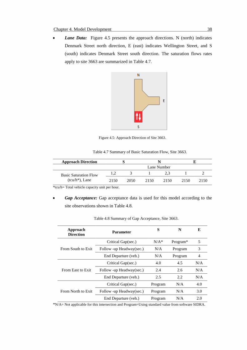
Chapter 4. Model Development 38
Lane Data: Figure 4.5 presents the approach directions. N (north) indicates
Denmark Street north direction, E (east) indicates Wellington Street, and S
(south) indicates Denmark Street south direction. The saturation flows rates
apply to site 3663 are summarized in Table 4.7.
Figure 4.5: Approach Direction of Site 3663.
Table 4.7 Summary of Basic Saturation Flow, Site 3663.
Approach Direction S N E
Lane Number
Basic Saturation Flow
(tcu/h*), Lane
1,2 3 1 2,3 1 2
2150 2050 2150 2150 2150 2150
*tcu/h= Total vehicle capacity unit per hour.
Gap Acceptance: Gap acceptance data is used for this model according to the
site observations shown in Table 4.8.
Table 4.8 Summary of Gap Acceptance, Site 3663.
Approach
Direction Parameter
S
N
E
From South to Exit
Critical Gap(sec.) N/A* Program* 5
Follow -up Headway(sec.) N/A Program 3
End Departure (veh.) N/A Program 4
From East to Exit
Critical Gap(sec.) 4.0 4.5 N/A
Follow -up Headway(sec.) 2.4 2.6 N/A
End Departure (veh.) 2.5 2.2 N/A
From North to Exit
Critical Gap(sec.) Program N/A 4.0
Follow -up Headway(sec.) Program N/A 3.0
End Departure (veh.) Program N/A 2.0
*N/A= Not applicable for this intersection and Program=Using standard value from software SIDRA.
Chapter 4. Model Development 39
Vehicle Movement Data: The path and signal data collected from the survey
are plotted to model the corridor. Table 4.9 shows the data summary.
Table 4.9 Summary of Signal Data, Site 3663.
Approach Direction Parameter S
N
E
From South to Exit Approach Cruise Speed (km/h.) N/A* 48 40
Exit Cruise Speed (km/h.) N/A 45 32
Start Loss (sec.) N/A 0 6
End Loss (sec.) N/A 0 0
From East to Exit Approach Cruise Speed (km/h.) 48 55 N/A
Exit Cruise Speed (km/h.) 43 40 N/A
Start Loss (sec.) 3 0 N/A
End Loss (sec.) 0 0 N/A
From North to Exit Approach Cruise Speed (km/h.) 48 N/A 49
Exit Cruise Speed (km/h.) 40 N/A 40
Start Loss (sec.) 6 N/A 0
End Loss (sec.) 0 N/A 0
*N/A= Not applicable for this intersection.
Phasing and Timing: This intersection is a variable eight-phase intersection.
The data sets collected from VicRoads are applied. A practical cycle time is
selected for modelling.
Table 4.10 Summary of a Signal Cycle Phase, Site 3663.
Phase A B B2 C D E1 E2 F
Phase Time (optional) (sec.) 0 0 0 0 0 0 0 0
Yellow time (sec.) 4 3 3 4 3 3 4 3
All-Red time (sec.) 2 2 2 2 2 2 2 2
Movement Definition, Lane Geometry, Pedestrian Traffic Volume, Traffic
Priority, Output result format settings & Model Settings: For these parameters
the same procedure as for site 3662 were used.
After inputting all parameters, the tab PROCESS is applied to output the results.
4.3.3 Intersection of Denmark Street/ Stevenson Street (Site 1190)
Intersection of Denmark Street/ Stevenson Street a signalised T-intersection and each
direction have two-way lanes. Denmark Street and Stevenson Street have full-length
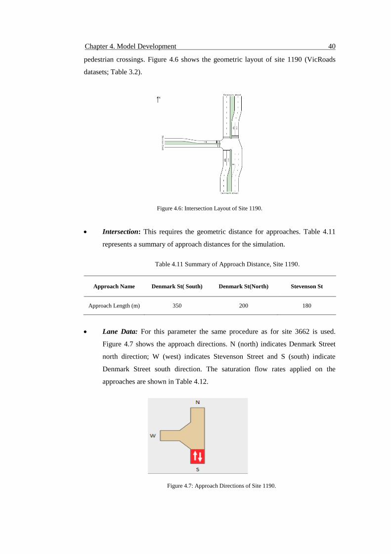
Chapter 4. Model Development 40
pedestrian crossings. Figure 4.6 shows the geometric layout of site 1190 (VicRoads
datasets; Table 3.2).
Figure 4.6: Intersection Layout of Site 1190.
Intersection: This requires the geometric distance for approaches. Table 4.11
represents a summary of approach distances for the simulation.
Table 4.11 Summary of Approach Distance, Site 1190.
Approach Name Denmark St( South) Denmark St(North) Stevenson St
Approach Length (m) 350 200 180
Lane Data: For this parameter the same procedure as for site 3662 is used.
Figure 4.7 shows the approach directions. N (north) indicates Denmark Street
north direction; W (west) indicates Stevenson Street and S (south) indicate
Denmark Street south direction. The saturation flow rates applied on the
approaches are shown in Table 4.12.
Figure 4.7: Approach Directions of Site 1190.
Chapter 4. Model Development 41
Table 4.12 Summary of Basic Saturation Flow, Site 1190.
Approach Direction S N W
Lane Number
Basic Saturation Flow
(tcu/h), Lane
1 2 1 2 1
1950 1950 1950 1950 2250
*tcu/h= Total vehicle capacity unit per hour.
Gap Acceptance: Gap acceptance data are used for this model according to the
site observations presented in Table 4.13.
Table 4.13 Summary of Gap Acceptance, Site 1190.
Approach
Direction
Parameter S
N
W
From South to
Exit
Critical Gap (sec.) N/A* 0.0 Program*
Follow-up Headway (sec.) N/A 0.0 Program
End Departure (veh.) N/A 0.0 Program
From West to Exit Critical Gap (sec.) 4.5 4.0 N/A
Follow -up Headway (sec.) 2.4 2.4 N/A
End Departure (veh.) 2.5 2.5 N/A
From North to
Exit
Critical Gap (sec.) 0.0 N/A 4.5
Follow -up Headway (sec.) 0.0 N/A 2.6
End Departure (veh.) 0.0 N/A 2.2
*N/A= Not applicable for this intersection and Program=Using standard value from software SIDRA.
Vehicle Movement Data: Signal data collected from Surveys are plotted to
model the corridor. Table 4.14 presents the summarized data for all speeds.
Table 4.14 Summary of Signal Data, Site 1190.
Approach Direction Parameter S
N
W
From South to Exit
Approach Cruise Speed (km/h.) N/A* 50 50
Exit Cruise Speed (km/h.) N/A 40 40
Start Loss (sec.) N/A 0 0
End Loss (sec.) N/A 0 0
From West to Exit
Approach Cruise Speed (km/h.) 50 50 N/A
Exit Cruise Speed (km/h.) 45 45 N/A
Start Loss (sec.) 0 0 N/A
End Loss (sec.) 4 4 N/A
From North to Exit
Approach Cruise Speed (km/h.) 50 N/A 50
Exit Cruise Speed (km/h.) 45 N/A 45
Start Loss (sec.) 0 N/A 0
End Loss (sec.) 0 N/A 0
*N/A= Not applicable for this intersection.
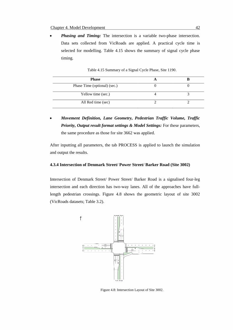
Chapter 4. Model Development 42
Phasing and Timing: The intersection is a variable two-phase intersection.
Data sets collected from VicRoads are applied. A practical cycle time is
selected for modelling. Table 4.15 shows the summary of signal cycle phase
timing.
Table 4.15 Summary of a Signal Cycle Phase, Site 1190.
Phase A B
Phase Time (optional) (sec.) 0 0
Yellow time (sec.) 4 3
All Red time (sec) 2 2
Movement Definition, Lane Geometry, Pedestrian Traffic Volume, Traffic
Priority, Output result format settings & Model Settings: For these parameters,
the same procedure as those for site 3662 was applied.
After inputting all parameters, the tab PROCESS is applied to launch the simulation
and output the results.
4.3.4 Intersection of Denmark Street/ Power Street/ Barker Road (Site 3002)
Intersection of Denmark Street/ Power Street/ Barker Road is a signalised four-leg
intersection and each direction has two-way lanes. All of the approaches have full-
length pedestrian crossings. Figure 4.8 shows the geometric layout of site 3002
(VicRoads datasets; Table 3.2).
Figure 4.8: Intersection Layout of Site 3002.
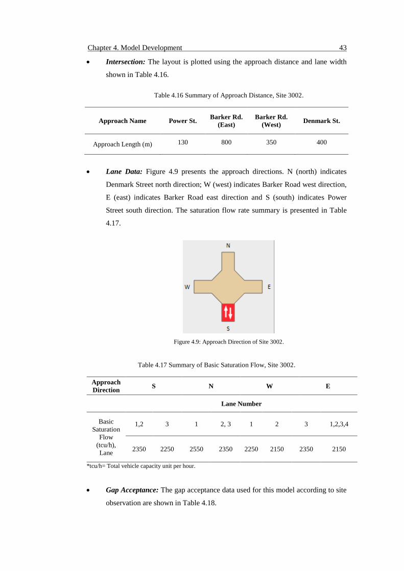
Chapter 4. Model Development 43
Intersection: The layout is plotted using the approach distance and lane width
shown in Table 4.16.
Table 4.16 Summary of Approach Distance, Site 3002.
Approach Name Power St. Barker Rd.
(East)
Barker Rd.
(West) Denmark St.
Approach Length (m) 130 800 350 400
Lane Data: Figure 4.9 presents the approach directions. N (north) indicates
Denmark Street north direction; W (west) indicates Barker Road west direction,
E (east) indicates Barker Road east direction and S (south) indicates Power
Street south direction. The saturation flow rate summary is presented in Table
4.17.
Figure 4.9: Approach Direction of Site 3002.
Table 4.17 Summary of Basic Saturation Flow, Site 3002.
Approach
Direction S N W E
Lane Number
Basic
Saturation
Flow
(tcu/h),
Lane
1,2 3 1 2, 3 1 2 3 1,2,3,4
2350 2250 2550 2350 2250 2150 2350 2150
*tcu/h= Total vehicle capacity unit per hour.
Gap Acceptance: The gap acceptance data used for this model according to site
observation are shown in Table 4.18.
Chapter 4. Model Development 44
Table 4.18 Summary of Gap Acceptance, Site 3002.
Approach
Direction Parameter
S
N
W
E
From South to
Exit
Critical Gap (sec.) N/A* 0.0 Program* 2.0
Follow-up Headway (sec) N/A 0.0 Program 1.50
End Departure (veh.) N/A 0.0 Program 2.2
From East to
Exit
Critical Gap (sec.) 4.0 4.5 1.0 N/A
Follow-up Headway(sec) 2.4 2.6 0.50 N/A
End Departure (veh.) 2.5 2.2 0.1 N/A
From North to
Exit
Critical Gap (sec.) 0.0 N/A 2.0 1.0
Follow-up Headway(sec) 0.0 N/A 1.50 0.50
End Departure (veh.) 0.0 N/A 2.20 0.10
From West to
Exit
Critical Gap (sec.) 2.0 1.0 N/A Program
Follow-up Headway(sec) 1.50 0.50 N/A Program
End Departure (veh.) 0.1 0.1 N/A Program
*N/A= Not applicable for this intersection and Program=Using standard value from software SIDRA.
Vehicle Movement Data: The signal data collected from the Survey were
plotted to model the corridor. A summary of plotted data is presented in Table
4.19.
Table 4.19 Summary Signal Data, Site 3002.
Approach
Direction Parameter S
N
W
E
From South to
Exit
Approach Cruise Speed (km/h.) N/A* 55 55 55
Exit Cruise Speed (km/h.) N/A 50 50 55
Start Loss (sec.) N/A 0 0 0
End Loss (sec.) N/A 6 6 4
From East to Exit
Approach Cruise Speed (km/h.) 56 55 55 N/A
Exit Cruise Speed (km/h.) 52 45 50 N/A
Start Loss (sec.) 0 0 0 N/A
End Loss (sec.) 3 0 0 N/A
From North to
Exit
Approach Cruise Speed (km/h.) 55 N/A 55 60
Exit Cruise Speed (km/h.) 50 N/A 55 58
Start Loss (sec.) 0 N/A 0 0
End Loss (sec.) 0 N/A 10 4
From West to
Exit
Approach Cruise Speed (km/h.) 55 55 N/A 50
Exit Cruise Speed (km/h.) 50 50 N/A 45
Start Loss (sec.) 0 0 N/A 0
End Loss (sec.) 0 3 N/A 0
*N/A= Not applicable for this intersection
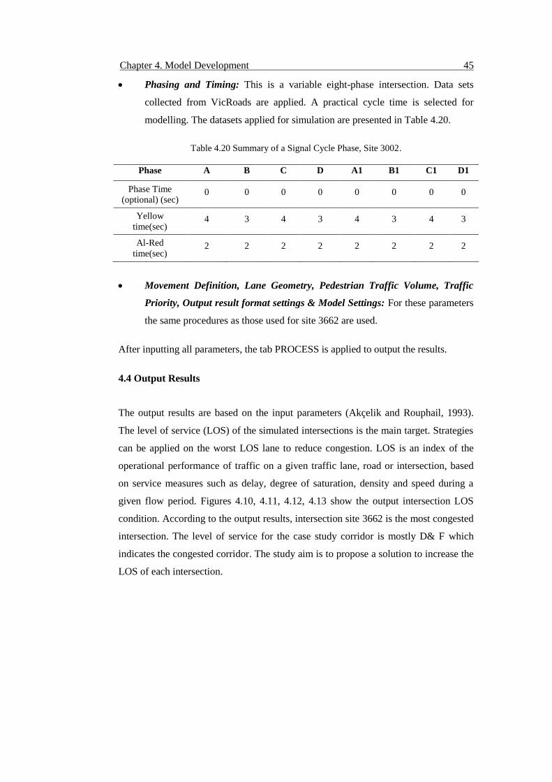
Chapter 4. Model Development 45
Phasing and Timing: This is a variable eight-phase intersection. Data sets
collected from VicRoads are applied. A practical cycle time is selected for
modelling. The datasets applied for simulation are presented in Table 4.20.
Table 4.20 Summary of a Signal Cycle Phase, Site 3002.
Phase A B C D A1 B1 C1 D1
Phase Time
(optional) (sec) 0 0 0 0 0 0 0 0
Yellow
time(sec) 4 3 4 3 4 3 4 3
Al-Red
time(sec) 2 2 2 2 2 2 2 2
Movement Definition, Lane Geometry, Pedestrian Traffic Volume, Traffic
Priority, Output result format settings & Model Settings: For these parameters
the same procedures as those used for site 3662 are used.
After inputting all parameters, the tab PROCESS is applied to output the results.
4.4 Output Results
The output results are based on the input parameters (Akçelik and Rouphail, 1993).
The level of service (LOS) of the simulated intersections is the main target. Strategies
can be applied on the worst LOS lane to reduce congestion. LOS is an index of the
operational performance of traffic on a given traffic lane, road or intersection, based
on service measures such as delay, degree of saturation, density and speed during a
given flow period. Figures 4.10, 4.11, 4.12, 4.13 show the output intersection LOS
condition. According to the output results, intersection site 3662 is the most congested
intersection. The level of service for the case study corridor is mostly D& F which
indicates the congested corridor. The study aim is to propose a solution to increase the
LOS of each intersection.
Chapter 4. Model Development 46
Figure 4.10: LOS Layout of Site 3662.

Chapter 4. Model Development 47
Figure 4.11: LOS Layout of Site 3663.
Figure 4.12: LOS Layout of Site 1190.
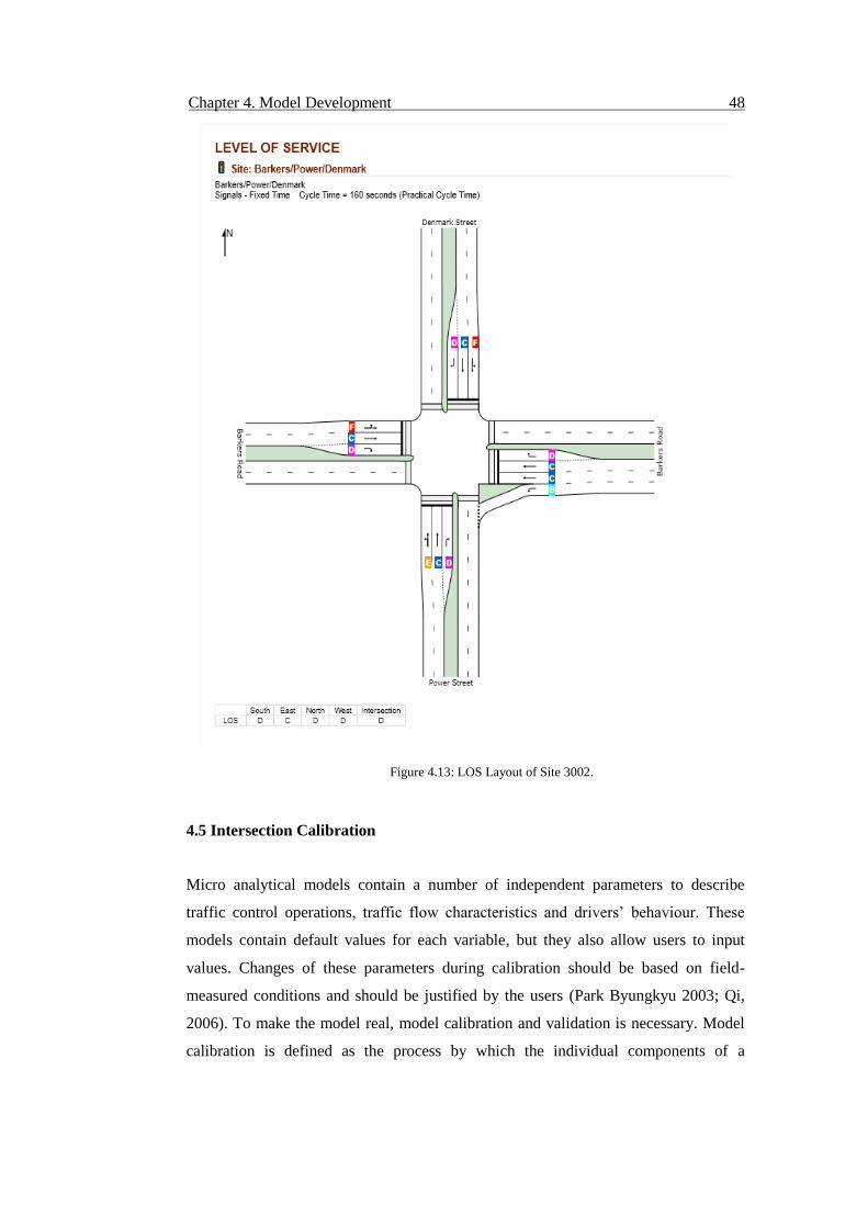
Chapter 4. Model Development 48
Figure 4.13: LOS Layout of Site 3002.
4.5 Intersection Calibration
Micro analytical models contain a number of independent parameters to describe
traffic control operations, traffic flow characteristics and drivers’ behaviour. These
models contain default values for each variable, but they also allow users to input
values. Changes of these parameters during calibration should be based on field-
measured conditions and should be justified by the users (Park Byungkyu 2003; Qi,
2006). To make the model real, model calibration and validation is necessary. Model
calibration is defined as the process by which the individual components of a
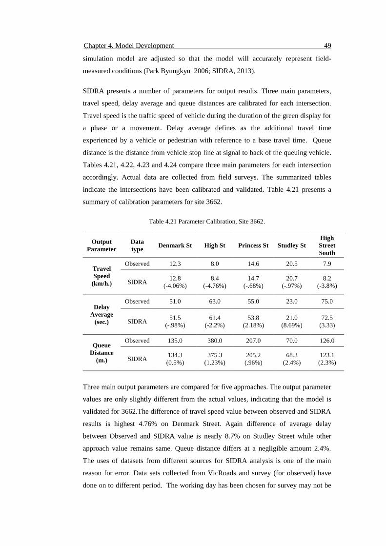
Chapter 4. Model Development 49
simulation model are adjusted so that the model will accurately represent field-
measured conditions (Park Byungkyu 2006; SIDRA, 2013).
SIDRA presents a number of parameters for output results. Three main parameters,
travel speed, delay average and queue distances are calibrated for each intersection.
Travel speed is the traffic speed of vehicle during the duration of the green display for
a phase or a movement. Delay average defines as the additional travel time
experienced by a vehicle or pedestrian with reference to a base travel time. Queue
distance is the distance from vehicle stop line at signal to back of the queuing vehicle.
Tables 4.21, 4.22, 4.23 and 4.24 compare three main parameters for each intersection
accordingly. Actual data are collected from field surveys. The summarized tables
indicate the intersections have been calibrated and validated. Table 4.21 presents a
summary of calibration parameters for site 3662.
Table 4.21 Parameter Calibration, Site 3662.
Output
Parameter
Data
type Denmark St High St Princess St Studley St
High
Street
South
Travel
Speed
(km/h.)
Observed 12.3 8.0 14.6 20.5 7.9
SIDRA 12.8
(-4.06%)
8.4
(-4.76%)
14.7
(-.68%)
20.7
(-.97%)
8.2
(-3.8%)
Delay
Average
(sec.)
Observed 51.0 63.0 55.0 23.0 75.0
SIDRA 51.5
(-.98%)
61.4
(-2.2%)
53.8
(2.18%)
21.0
(8.69%)
72.5
(3.33)
Queue
Distance
(m.)
Observed 135.0 380.0 207.0 70.0 126.0
SIDRA 134.3
(0.5%)
375.3
(1.23%)
205.2
(.96%)
68.3
(2.4%)
123.1
(2.3%)
Three main output parameters are compared for five approaches. The output parameter
values are only slightly different from the actual values, indicating that the model is
validated for 3662.The difference of travel speed value between observed and SIDRA
results is highest 4.76% on Denmark Street. Again difference of average delay
between Observed and SIDRA value is nearly 8.7% on Studley Street while other
approach value remains same. Queue distance differs at a negligible amount 2.4%.
The uses of datasets from different sources for SIDRA analysis is one of the main
reason for error. Data sets collected from VicRoads and survey (for observed) have
done on to different period. The working day has been chosen for survey may not be
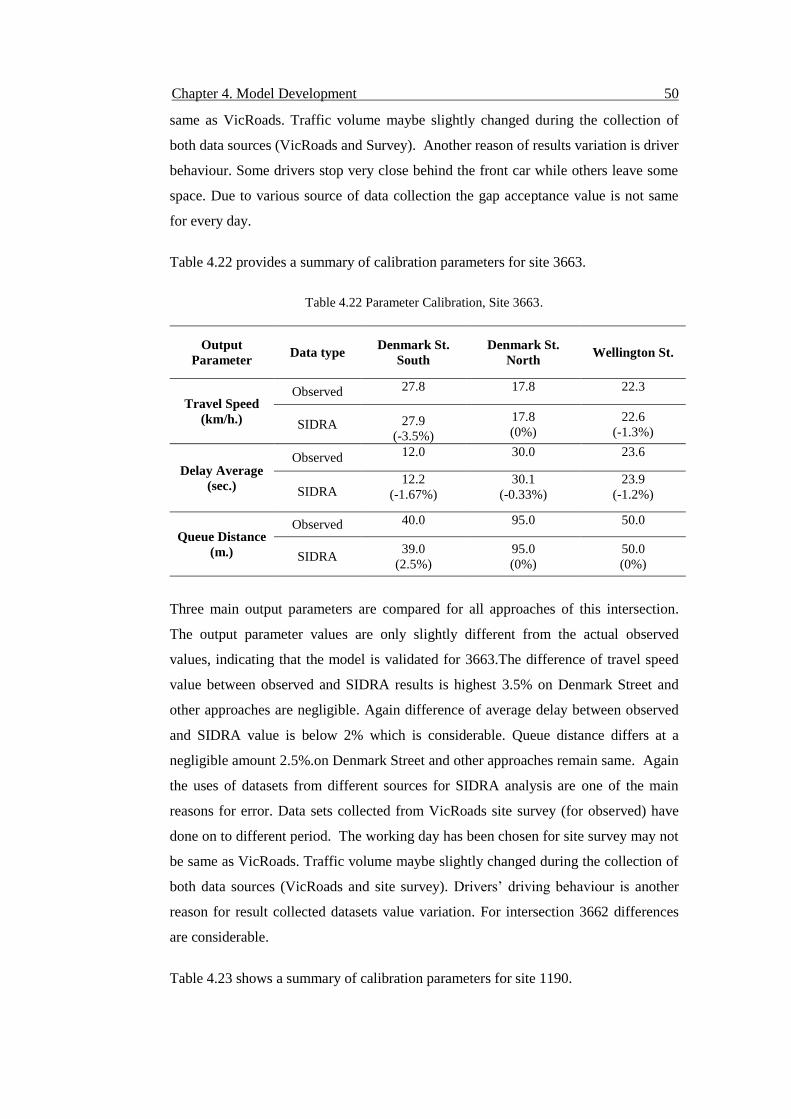
Chapter 4. Model Development 50
same as VicRoads. Traffic volume maybe slightly changed during the collection of
both data sources (VicRoads and Survey). Another reason of results variation is driver
behaviour. Some drivers stop very close behind the front car while others leave some
space. Due to various source of data collection the gap acceptance value is not same
for every day.
Table 4.22 provides a summary of calibration parameters for site 3663.
Table 4.22 Parameter Calibration, Site 3663.
Output
Parameter Data type
Denmark St.
South
Denmark St.
North Wellington St.
Travel Speed
(km/h.)
Observed 27.8 17.8 22.3
SIDRA 27.9
(-3.5%)
17.8
(0%)
22.6
(-1.3%)
Delay Average
(sec.)
Observed 12.0
30.0 23.6
SIDRA 12.2
(-1.67%)
30.1
(-0.33%)
23.9
(-1.2%)
Queue Distance
(m.)
Observed 40.0 95.0 50.0
SIDRA 39.0
(2.5%)
95.0
(0%)
50.0
(0%)
Three main output parameters are compared for all approaches of this intersection.
The output parameter values are only slightly different from the actual observed
values, indicating that the model is validated for 3663.The difference of travel speed
value between observed and SIDRA results is highest 3.5% on Denmark Street and
other approaches are negligible. Again difference of average delay between observed
and SIDRA value is below 2% which is considerable. Queue distance differs at a
negligible amount 2.5%.on Denmark Street and other approaches remain same. Again
the uses of datasets from different sources for SIDRA analysis are one of the main
reasons for error. Data sets collected from VicRoads site survey (for observed) have
done on to different period. The working day has been chosen for site survey may not
be same as VicRoads. Traffic volume maybe slightly changed during the collection of
both data sources (VicRoads and site survey). Drivers’ driving behaviour is another
reason for result collected datasets value variation. For intersection 3662 differences
are considerable.
Table 4.23 shows a summary of calibration parameters for site 1190.

Chapter 4. Model Development 51
Table 4.23 Parameter Calibration, Site 1190.
Output
Parameter Data type
Denmark St.
South
Denmark St.
North Stevenson St.
Travel Speed
(km/h.)
Observed 34.0 25.0 28.6
SIDRA 34.1
(-.3%)
25.0
(0%)
28.7
(-.34%)
Delay
Average(sec.)
Observed 12.0 16.8 15.0
SIDRA 12.3
(-2.5%)
16.8
(%)
15.1
(-0.66%)
Queue Distance
(m.)
Observed 50.0 125.0 8.0
SIDRA 49.0
(2%)
122.0
(2.4%)
8.0
(%)
The output parameter values are only slightly different from the actual values,
indicating that the model is validated for intersection 1190. The difference of travel
speed value between observed and SIDRA results are highest 0.35% on Stevenson
Street which is negligible. Again difference of average delay between observed and
SIDRA value is 2.5% and other approaches remain same with a small difference.
Queue distance differs at a negligible amount 2.5% on Denmark Street North while
other approaches differ less than 2.5%. Followed by intersection 3662 and 3663 uses
of datasets from different sources for SIDRA analysis is one of the main reasons for
error of intersection 1190. Driving behaviour is another reason for result variation.
Table 4.24 presents a summary of calibration parameters for site 3002.
Table 4.24 Parameter Calibration, Site 3002.
Output
Parameter Data type Power St.
Barker Rd.
East
Barker Rd.
West
Denmark
St.
Travel
Speed
(km/h.)
Observed 14.8 35.4 21.0 18.6
SIDRA 14.9
(-.67%)
35.4
(0%)
21.3
(-1.4%)
18.6
(0%)
Delay
Average
(sec.)
Observed 35.8 29.6 43.8 53.5
SIDRA 35.9
(-.27%)
29.8
(-.67%)
43.8
(0%)
53.5
(0%)
Queue
Distance
(m.)
Observed 120 125 86 190
SIDRA 120
(0%)
125
(%)
87
(-1.16%)
190
(0%)
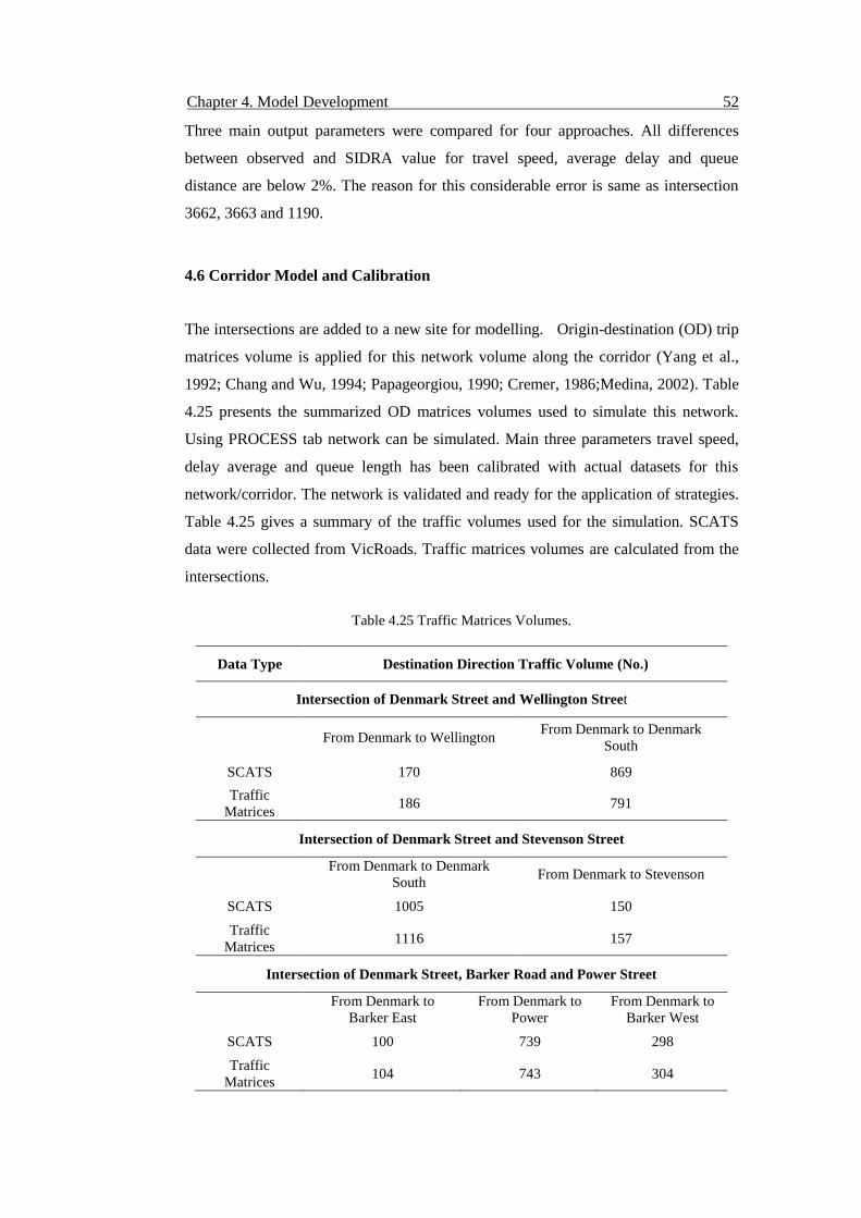
Chapter 4. Model Development 52
Three main output parameters were compared for four approaches. All differences
between observed and SIDRA value for travel speed, average delay and queue
distance are below 2%. The reason for this considerable error is same as intersection
3662, 3663 and 1190.
4.6 Corridor Model and Calibration
The intersections are added to a new site for modelling. Origin-destination (OD) trip
matrices volume is applied for this network volume along the corridor (Yang et al.,
1992; Chang and Wu, 1994; Papageorgiou, 1990; Cremer, 1986;Medina, 2002). Table
4.25 presents the summarized OD matrices volumes used to simulate this network.
Using PROCESS tab network can be simulated. Main three parameters travel speed,
delay average and queue length has been calibrated with actual datasets for this
network/corridor. The network is validated and ready for the application of strategies.
Table 4.25 gives a summary of the traffic volumes used for the simulation. SCATS
data were collected from VicRoads. Traffic matrices volumes are calculated from the
intersections.
Table 4.25 Traffic Matrices Volumes.
Data Type Destination Direction Traffic Volume (No.)
Intersection of Denmark Street and Wellington Street
From Denmark to Wellington From Denmark to Denmark
South
SCATS 170 869
Traffic
Matrices 186 791
Intersection of Denmark Street and Stevenson Street
From Denmark to Denmark
South From Denmark to Stevenson
SCATS 1005 150
Traffic
Matrices 1116 157
Intersection of Denmark Street, Barker Road and Power Street
From Denmark to
Barker East
From Denmark to
Power
From Denmark to
Barker West
SCATS 100 739 298
Traffic
Matrices 104 743 304
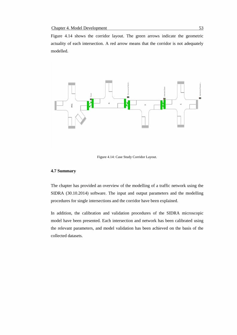
Chapter 4. Model Development 53
Figure 4.14 shows the corridor layout. The green arrows indicate the geometric
actuality of each intersection. A red arrow means that the corridor is not adequately
modelled.
Figure 4.14: Case Study Corridor Layout.
4.7 Summary
The chapter has provided an overview of the modelling of a traffic network using the
SIDRA (30.10.2014) software. The input and output parameters and the modelling
procedures for single intersections and the corridor have been explained.
In addition, the calibration and validation procedures of the SIDRA microscopic
model have been presented. Each intersection and network has been calibrated using
the relevant parameters, and model validation has been achieved on the basis of the
collected datasets.
54
Chapter 5
Applied Strategies
5.1 Introduction
In this chapter the strategies applied to the case study Melbourne traffic corridor are
explained. The results of traffic measurements (e.g. Travel speed, Queue distance and
Average delay) after the application of each strategy are presented and discussed. The
chapter also identifies the best options to resolve congestion for this case study
corridor.
5.2 Strategies applied to reduce congestion
In the literature review, modal management strategies are classified in different ways.
Various strategies have been applied in previous studies according to case study type.
The strategies which could be applied on this corridor are as follows:
Priority for buses and trams
Signal priority for buses and trams involves vehicle detectors being installed at
intersections. Whenever a bus or tram nears the detector the signal changes to green
for that particular direction. The application of this strategy means that public
transport can have priority over other traffic.
Remove bicycle lanes
Bicycle lanes can be removed and other existing vehicle lanes can be narrowed. More
lanes can operate by adopting this strategy. As a result, vehicles moving towards exits
have more lanes and space to clear intersections quickly.
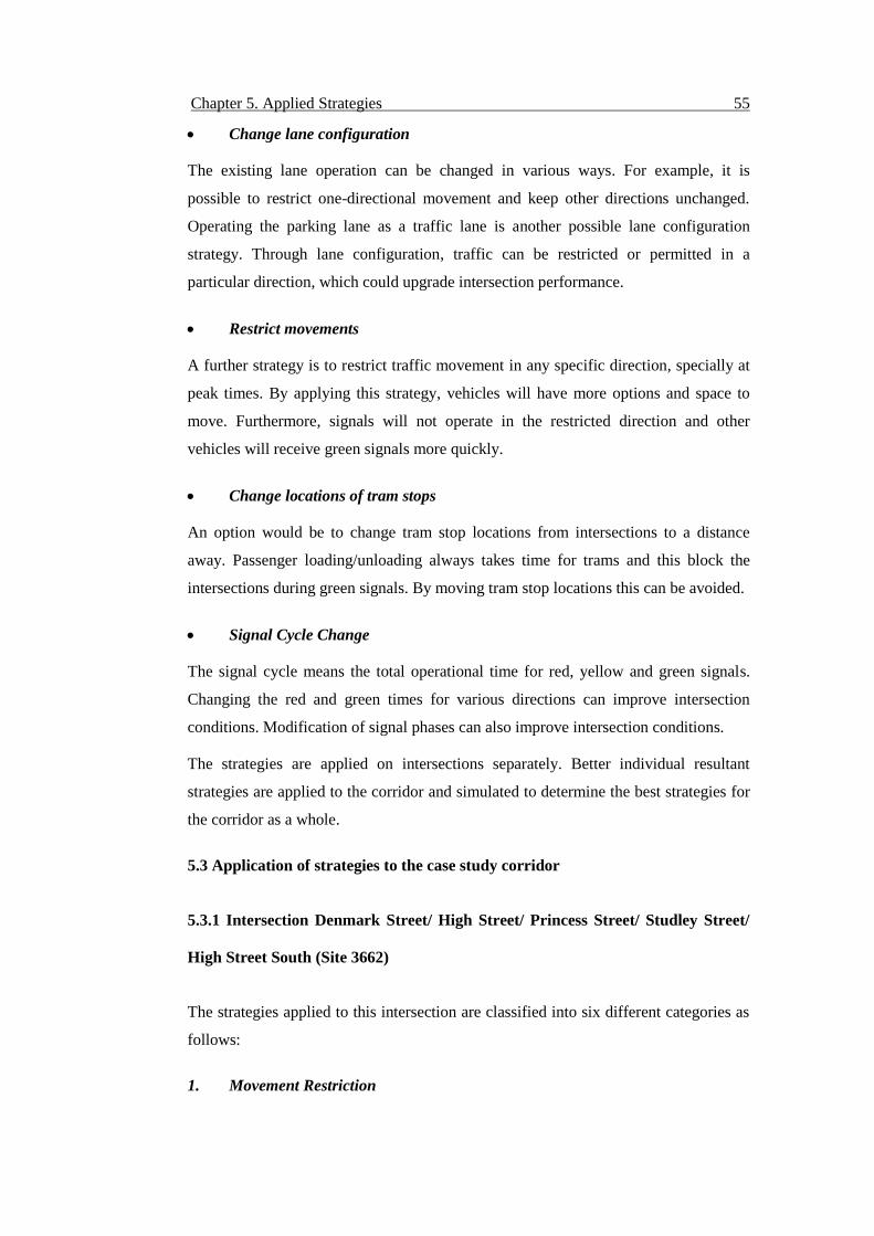
Chapter 5. Applied Strategies 55
Change lane configuration
The existing lane operation can be changed in various ways. For example, it is
possible to restrict one-directional movement and keep other directions unchanged.
Operating the parking lane as a traffic lane is another possible lane configuration
strategy. Through lane configuration, traffic can be restricted or permitted in a
particular direction, which could upgrade intersection performance.
Restrict movements
A further strategy is to restrict traffic movement in any specific direction, specially at
peak times. By applying this strategy, vehicles will have more options and space to
move. Furthermore, signals will not operate in the restricted direction and other
vehicles will receive green signals more quickly.
Change locations of tram stops
An option would be to change tram stop locations from intersections to a distance
away. Passenger loading/unloading always takes time for trams and this block the
intersections during green signals. By moving tram stop locations this can be avoided.
Signal Cycle Change
The signal cycle means the total operational time for red, yellow and green signals.
Changing the red and green times for various directions can improve intersection
conditions. Modification of signal phases can also improve intersection conditions.
The strategies are applied on intersections separately. Better individual resultant
strategies are applied to the corridor and simulated to determine the best strategies for
the corridor as a whole.
5.3 Application of strategies to the case study corridor
5.3.1 Intersection Denmark Street/ High Street/ Princess Street/ Studley Street/
High Street South (Site 3662)
The strategies applied to this intersection are classified into six different categories as
follows:
1. Movement Restriction
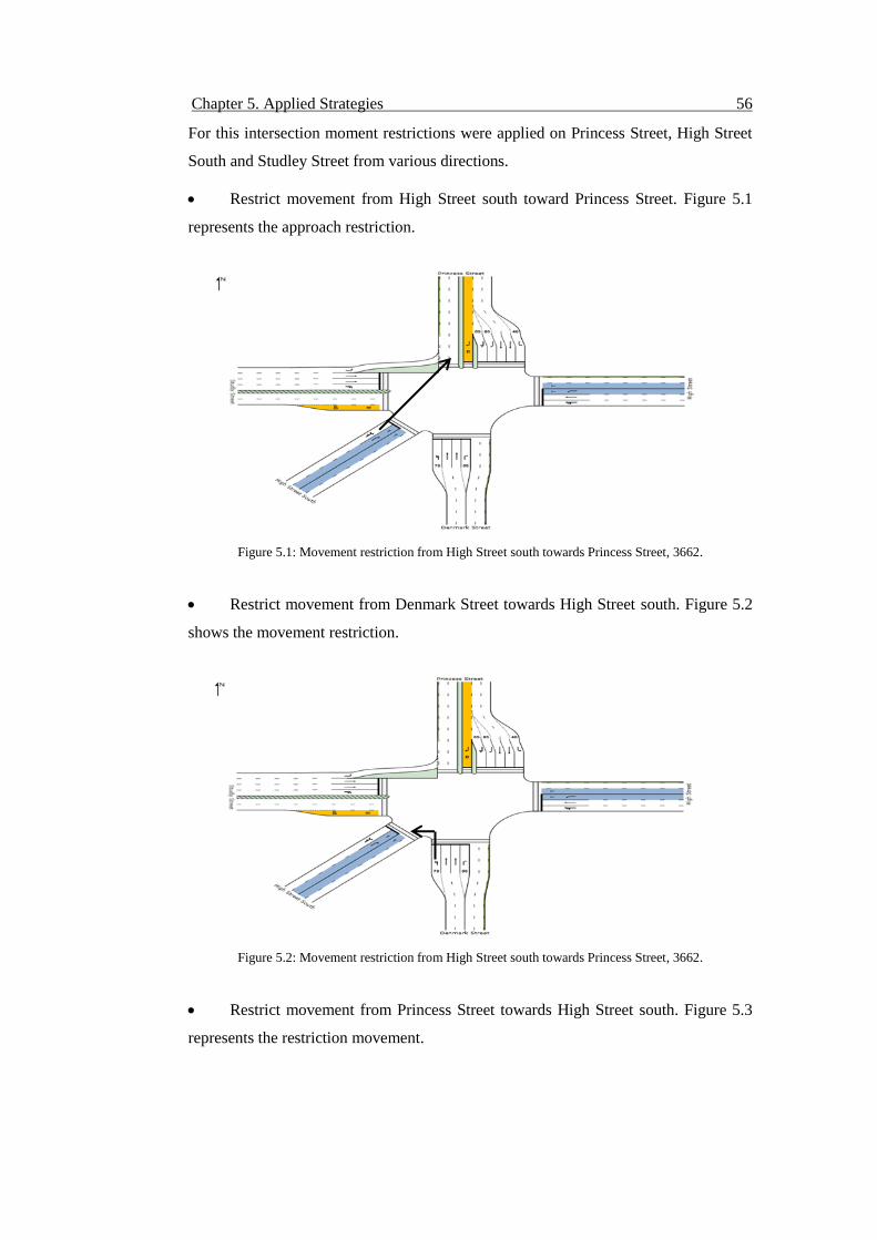
Chapter 5. Applied Strategies 56
For this intersection moment restrictions were applied on Princess Street, High Street
South and Studley Street from various directions.
Restrict movement from High Street south toward Princess Street. Figure 5.1
represents the approach restriction.
Figure 5.1: Movement restriction from High Street south towards Princess Street, 3662.
Restrict movement from Denmark Street towards High Street south. Figure 5.2
shows the movement restriction.
Figure 5.2: Movement restriction from High Street south towards Princess Street, 3662.
Restrict movement from Princess Street towards High Street south. Figure 5.3
represents the restriction movement.
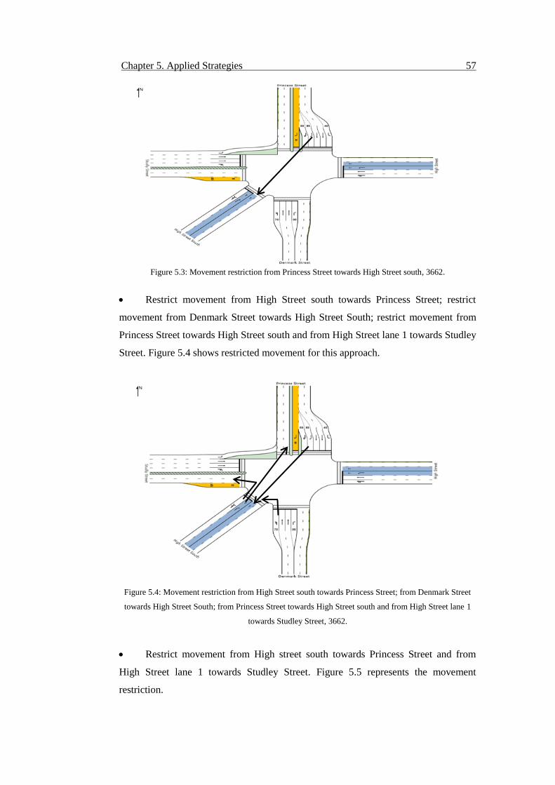
Chapter 5. Applied Strategies 57
Figure 5.3: Movement restriction from Princess Street towards High Street south, 3662.
Restrict movement from High Street south towards Princess Street; restrict
movement from Denmark Street towards High Street South; restrict movement from
Princess Street towards High Street south and from High Street lane 1 towards Studley
Street. Figure 5.4 shows restricted movement for this approach.
Figure 5.4: Movement restriction from High Street south towards Princess Street; from Denmark Street
towards High Street South; from Princess Street towards High Street south and from High Street lane 1
towards Studley Street, 3662.
Restrict movement from High street south towards Princess Street and from
High Street lane 1 towards Studley Street. Figure 5.5 represents the movement
restriction.
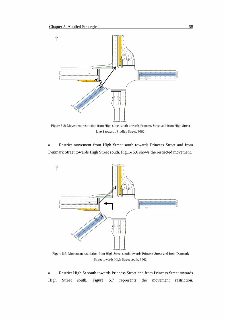
Chapter 5. Applied Strategies 58
Figure 5.5: Movement restriction from High street south towards Princess Street and from High Street
lane 1 towards Studley Street, 3662.
Restrict movement from High Street south towards Princess Street and from
Denmark Street towards High Street south. Figure 5.6 shows the restricted movement.
Figure 5.6: Movement restriction from High Street south towards Princess Street and from Denmark
Street towards High Street south, 3662.
Restrict High St south towards Princess Street and from Princess Street towards
High Street south. Figure 5.7 represents the movement restriction.
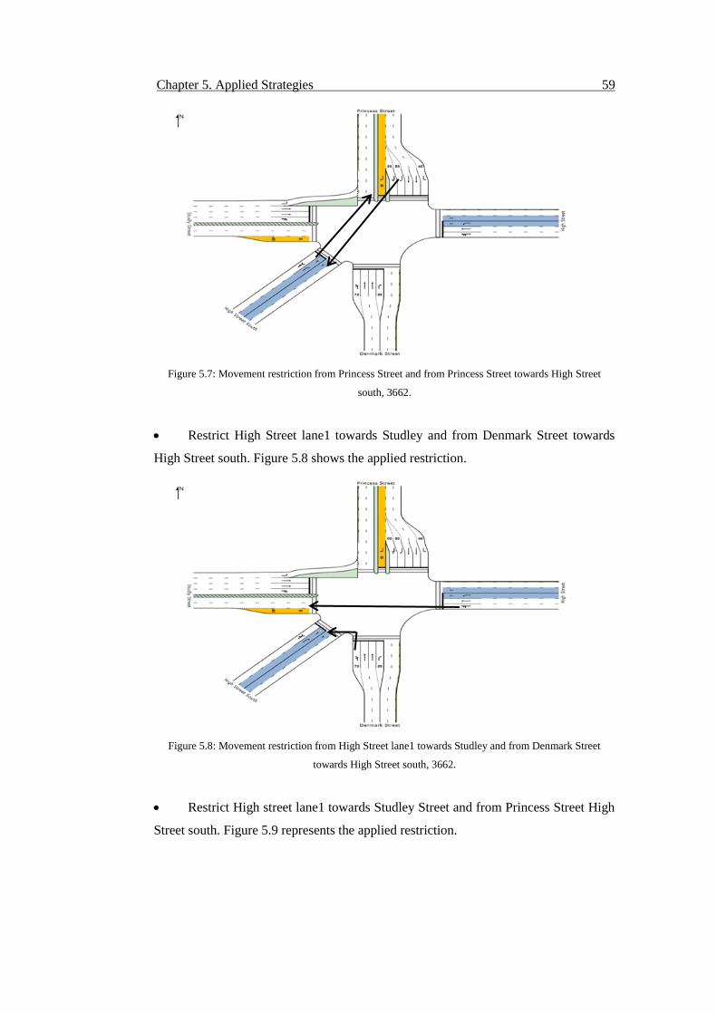
Chapter 5. Applied Strategies 59
Figure 5.7: Movement restriction from Princess Street and from Princess Street towards High Street
south, 3662.
Restrict High Street lane1 towards Studley and from Denmark Street towards
High Street south. Figure 5.8 shows the applied restriction.
Figure 5.8: Movement restriction from High Street lane1 towards Studley and from Denmark Street
towards High Street south, 3662.
Restrict High street lane1 towards Studley Street and from Princess Street High
Street south. Figure 5.9 represents the applied restriction.
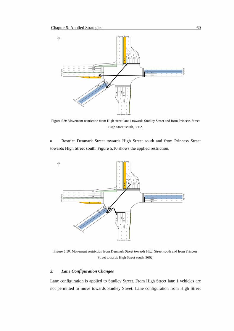
Chapter 5. Applied Strategies 60
Figure 5.9: Movement restriction from High street lane1 towards Studley Street and from Princess Street
High Street south, 3662.
Restrict Denmark Street towards High Street south and from Princess Street
towards High Street south. Figure 5.10 shows the applied restriction.
Figure 5.10: Movement restriction from Denmark Street towards High Street south and from Princess
Street towards High Street south, 3662.
2. Lane Configuration Changes
Lane configuration is applied to Studley Street. From High Street lane 1 vehicles are
not permitted to move towards Studley Street. Lane configuration from High Street
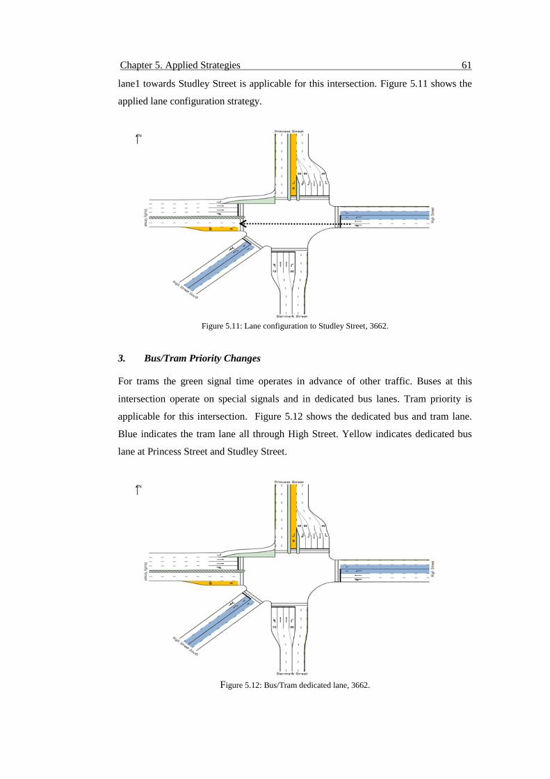
Chapter 5. Applied Strategies 61
lane1 towards Studley Street is applicable for this intersection. Figure 5.11 shows the
applied lane configuration strategy.
Figure 5.11: Lane configuration to Studley Street, 3662.
3. Bus/Tram Priority Changes
For trams the green signal time operates in advance of other traffic. Buses at this
intersection operate on special signals and in dedicated bus lanes. Tram priority is
applicable for this intersection. Figure 5.12 shows the dedicated bus and tram lane.
Blue indicates the tram lane all through High Street. Yellow indicates dedicated bus
lane at Princess Street and Studley Street.
Figure 5.12: Bus/Tram dedicated lane, 3662.
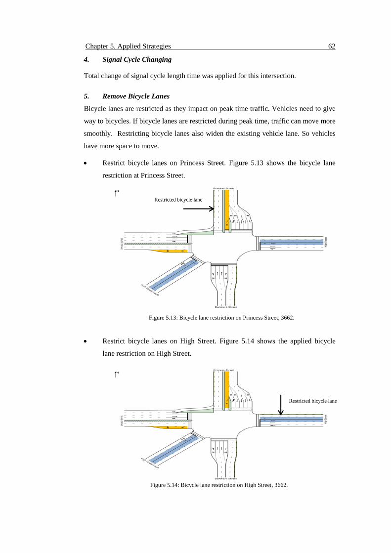
Chapter 5. Applied Strategies 62
4. Signal Cycle Changing
Total change of signal cycle length time was applied for this intersection.
5. Remove Bicycle Lanes
Bicycle lanes are restricted as they impact on peak time traffic. Vehicles need to give
way to bicycles. If bicycle lanes are restricted during peak time, traffic can move more
smoothly. Restricting bicycle lanes also widen the existing vehicle lane. So vehicles
have more space to move.
Restrict bicycle lanes on Princess Street. Figure 5.13 shows the bicycle lane
restriction at Princess Street.
Figure 5.13: Bicycle lane restriction on Princess Street, 3662.
Restrict bicycle lanes on High Street. Figure 5.14 shows the applied bicycle
lane restriction on High Street.
Figure 5.14: Bicycle lane restriction on High Street, 3662.
Restricted bicycle lane
Restricted bicycle lane
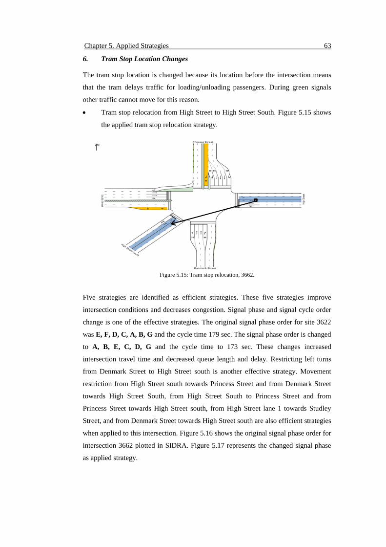
Chapter 5. Applied Strategies 63
6. Tram Stop Location Changes
The tram stop location is changed because its location before the intersection means
that the tram delays traffic for loading/unloading passengers. During green signals
other traffic cannot move for this reason.
Tram stop relocation from High Street to High Street South. Figure 5.15 shows
the applied tram stop relocation strategy.
Figure 5.15: Tram stop relocation, 3662.
Five strategies are identified as efficient strategies. These five strategies improve
intersection conditions and decreases congestion. Signal phase and signal cycle order
change is one of the effective strategies. The original signal phase order for site 3622
was E, F, D, C, A, B, G and the cycle time 179 sec. The signal phase order is changed
to A, B, E, C, D, G and the cycle time to 173 sec. These changes increased
intersection travel time and decreased queue length and delay. Restricting left turns
from Denmark Street to High Street south is another effective strategy. Movement
restriction from High Street south towards Princess Street and from Denmark Street
towards High Street South, from High Street South to Princess Street and from
Princess Street towards High Street south, from High Street lane 1 towards Studley
Street, and from Denmark Street towards High Street south are also efficient strategies
when applied to this intersection. Figure 5.16 shows the original signal phase order for
intersection 3662 plotted in SIDRA. Figure 5.17 represents the changed signal phase
as applied strategy.
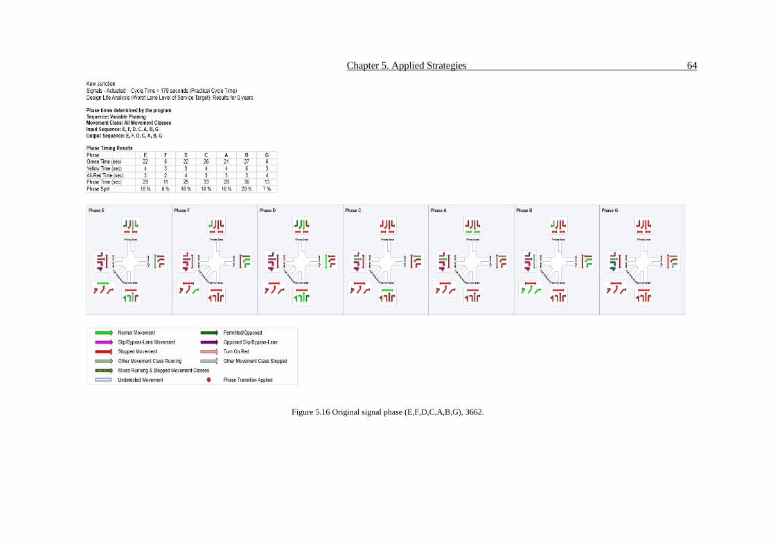
Chapter 5. Applied Strategies 64
Figure 5.16 Original signal phase (E,F,D,C,A,B,G), 3662.
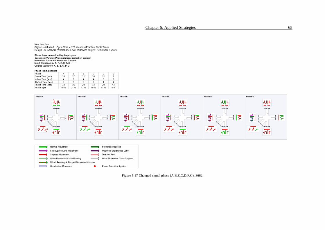
Chapter 5. Applied Strategies 65
Figure 5.17 Changed signal phase (A,B,E,C,D,F,G), 3662.
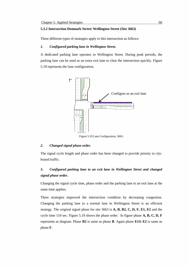
Chapter 5. Applied Strategies 66
5.3.2 Intersection Denmark Street/ Wellington Street (Site 3663)
Three different types of strategies apply to this intersection as follows:
1. Configured parking lane in Wellington Street.
A dedicated parking lane operates in Wellington Street. During peak periods, the
parking lane can be used as an extra exit lane to clear the intersection quickly. Figure
5.18 represents the lane configuration.
Figure 5.18 Lane Configuration, 3663.
2. Changed signal phase order.
The signal cycle length and phase order has been changed to provide priority to city-
bound traffic.
3. Configured parking lane to an exit lane in Wellington Street and changed
signal phase order.
Changing the signal cycle time, phase order and the parking lane to an exit lane at the
same time applies.
Three strategies improved the intersection condition by decreasing congestion.
Changing the parking lane to a normal lane in Wellington Street is an efficient
strategy. The original signal phase for site 3663 is A, B, B2, C, D, F, E1, E2 and the
cycle time 110 sec. Figure 5.19 shows the phase order. In figure phase A, B, C, D, F
represents as diagram. Phase B2 is same as phase B. Again phase E1& E2 is same as
phase F.
Configure as an exit lane
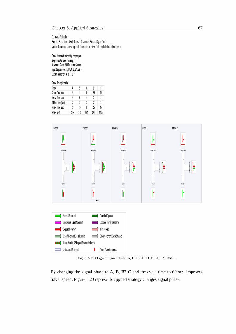
Chapter 5. Applied Strategies 67
Figure 5.19 Original signal phase (A, B, B2, C, D, F, E1, E2), 3663.
By changing the signal phase to A, B, B2 C and the cycle time to 60 sec. improves
travel speed. Figure 5.20 represents applied strategy changes signal phase.
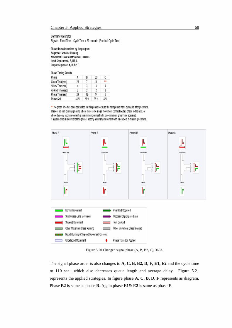
Chapter 5. Applied Strategies 68
Figure 5.20 Changed signal phase (A, B, B2, C), 3663.
The signal phase order is also changes to A, C, B, B2, D, F, E1, E2 and the cycle time
to 110 sec., which also decreases queue length and average delay. Figure 5.21
represents the applied strategies. In figure phase A, C, B, D, F represents as diagram.
Phase B2 is same as phase B. Again phase E1& E2 is same as phase F.
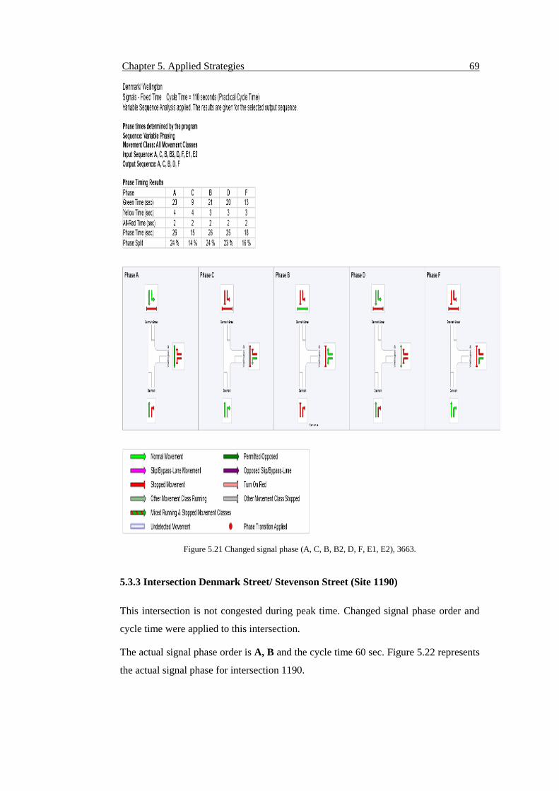
Chapter 5. Applied Strategies 69
Figure 5.21 Changed signal phase (A, C, B, B2, D, F, E1, E2), 3663.
5.3.3 Intersection Denmark Street/ Stevenson Street (Site 1190)
This intersection is not congested during peak time. Changed signal phase order and
cycle time were applied to this intersection.
The actual signal phase order is A, B and the cycle time 60 sec. Figure 5.22 represents
the actual signal phase for intersection 1190.
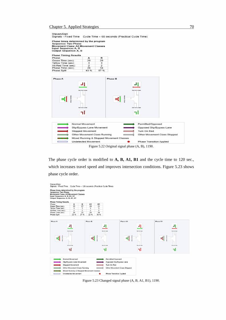
Chapter 5. Applied Strategies 70
Figure 5.22 Original signal phase (A, B), 1190.
The phase cycle order is modified to A, B, A1, B1 and the cycle time to 120 sec.,
which increases travel speed and improves intersection conditions. Figure 5.23 shows
phase cycle order.
Figure 5.23 Changed signal phase (A, B, A1, B1), 1190.
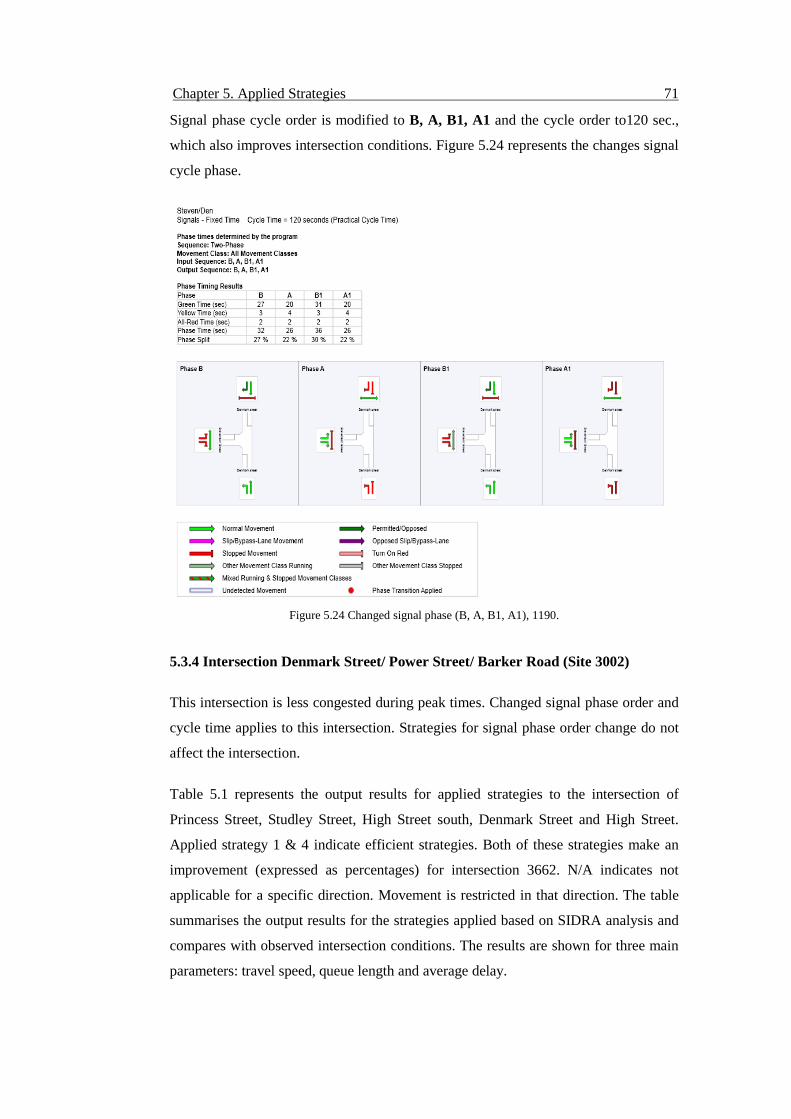
Chapter 5. Applied Strategies 71
Signal phase cycle order is modified to B, A, B1, A1 and the cycle order to120 sec.,
which also improves intersection conditions. Figure 5.24 represents the changes signal
cycle phase.
Figure 5.24 Changed signal phase (B, A, B1, A1), 1190.
5.3.4 Intersection Denmark Street/ Power Street/ Barker Road (Site 3002)
This intersection is less congested during peak times. Changed signal phase order and
cycle time applies to this intersection. Strategies for signal phase order change do not
affect the intersection.
Table 5.1 represents the output results for applied strategies to the intersection of
Princess Street, Studley Street, High Street south, Denmark Street and High Street.
Applied strategy 1 & 4 indicate efficient strategies. Both of these strategies make an
improvement (expressed as percentages) for intersection 3662. N/A indicates not
applicable for a specific direction. Movement is restricted in that direction. The table
summarises the output results for the strategies applied based on SIDRA analysis and
compares with observed intersection conditions. The results are shown for three main
parameters: travel speed, queue length and average delay.
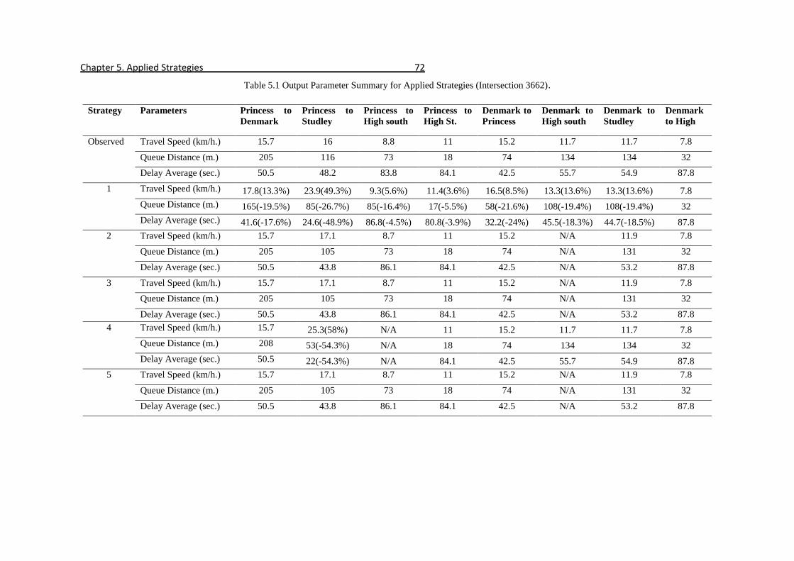
Chapter 5. Applied Strategies 72
Table 5.1 Output Parameter Summary for Applied Strategies (Intersection 3662).
Strategy Parameters Princess to
Denmark
Princess to
Studley
Princess to
High south
Princess to
High St.
Denmark to
Princess
Denmark to
High south
Denmark to
Studley
Denmark
to High
Observed Travel Speed (km/h.) 15.7 16 8.8 11 15.2 11.7 11.7 7.8
Queue Distance (m.) 205 116 73 18 74 134 134 32
Delay Average (sec.) 50.5 48.2 83.8 84.1 42.5 55.7 54.9 87.8
1 Travel Speed (km/h.) 17.8(13.3%) 23.9(49.3%) 9.3(5.6%) 11.4(3.6%) 16.5(8.5%) 13.3(13.6%) 13.3(13.6%) 7.8
Queue Distance (m.) 165(-19.5%) 85(-26.7%) 85(-16.4%) 17(-5.5%) 58(-21.6%) 108(-19.4%) 108(-19.4%) 32
Delay Average (sec.) 41.6(-17.6%) 24.6(-48.9%) 86.8(-4.5%) 80.8(-3.9%) 32.2(-24%) 45.5(-18.3%) 44.7(-18.5%) 87.8
2 Travel Speed (km/h.) 15.7 17.1 8.7 11 15.2 N/A 11.9 7.8
Queue Distance (m.) 205 105 73 18 74 N/A 131 32
Delay Average (sec.) 50.5 43.8 86.1 84.1 42.5 N/A 53.2 87.8
3 Travel Speed (km/h.) 15.7 17.1 8.7 11 15.2 N/A 11.9 7.8
Queue Distance (m.) 205 105 73 18 74 N/A 131 32
Delay Average (sec.) 50.5 43.8 86.1 84.1 42.5 N/A 53.2 87.8
4 Travel Speed (km/h.) 15.7 25.3(58%) N/A 11 15.2 11.7 11.7 7.8
Queue Distance (m.) 208 53(-54.3%) N/A 18 74 134 134 32
Delay Average (sec.) 50.5 22(-54.3%) N/A 84.1 42.5 55.7 54.9 87.8
5 Travel Speed (km/h.) 15.7 17.1 8.7 11 15.2 N/A 11.9 7.8
Queue Distance (m.) 205 105 73 18 74 N/A 131 32
Delay Average (sec.) 50.5 43.8 86.1 84.1 42.5 N/A 53.2 87.8
Chapter 5. Applied Strategies 73
Table 5.1 shows the improvement in percentages as a result of the strategies applied.
Percentages are calculated based on observed value and SIDRA analysis value using
the following equation using the following equation.
The application of strategy 1(changed signal cycle and phase order) increases travel
speed for intersection 3662 by up to 49%. This strategy shows the highest percentage
increase in travel speed for the approach starting from Princess Street towards Studley
Street. This approach operates towards the city. The modification of the signal phase
order and cycle time for this intersection creates less congestion during the morning
peak period. Queue distance and average delay decrease to 27% and 49%. On another
city-bound approach, Denmark Street towards High Street south, travel speed
increases by 14%, and queue distance and average speed decrease by 19% and 18 %.
Trams also run through High Street south. The application of strategy 1 improves
traffic conditions without hampering tram operations. Changing the signal cycle time
increases travel speed for other approaches to this intersection. The approach from
Denmark Street towards Studley Street is also city-bound. Changing the signal phase
order and cycle time improves travel speed by 13% with less queue distance and
delay. The approach travel speed is improved without hampering bus operations
through Studley Street.
Moreover, strategy 1 decreases the congestion of intersection 3662. Phase F has been
removed to modify signal phase order. On this phase F right turn active on Princess
Street. Movement from High street south towards Denmark Street and High Street is
also in operation. Tram is moving on this phase F as well (Figure 5.16). Removing
phase F during peak time also shorten the signal cycle phase which provides repetition
of green signal time more quickly. The most congested approach in this intersection is
High street specially the left lane (Lane1). From this lane vehicle is travelling on three
different directions (Denmark Street, High Street & Studley Street). At High street
from lane 2 (Middle lane) vehicles is travelling only on Studley Street. When the
signal is green for tram and lane one vehicles waiting on lane 2 cannot move. If any
vehicle traveling towards Studley Street waits on lane 1 on High street then other
vehicles behind it cannot move though it is green signal. It increases queue length and
delay. Modifying phase order by start with High street movement clear the
intersection congestion more quickly. During signal phase modification phase
transition applies for tram movement. Phase transition is a movement status where a
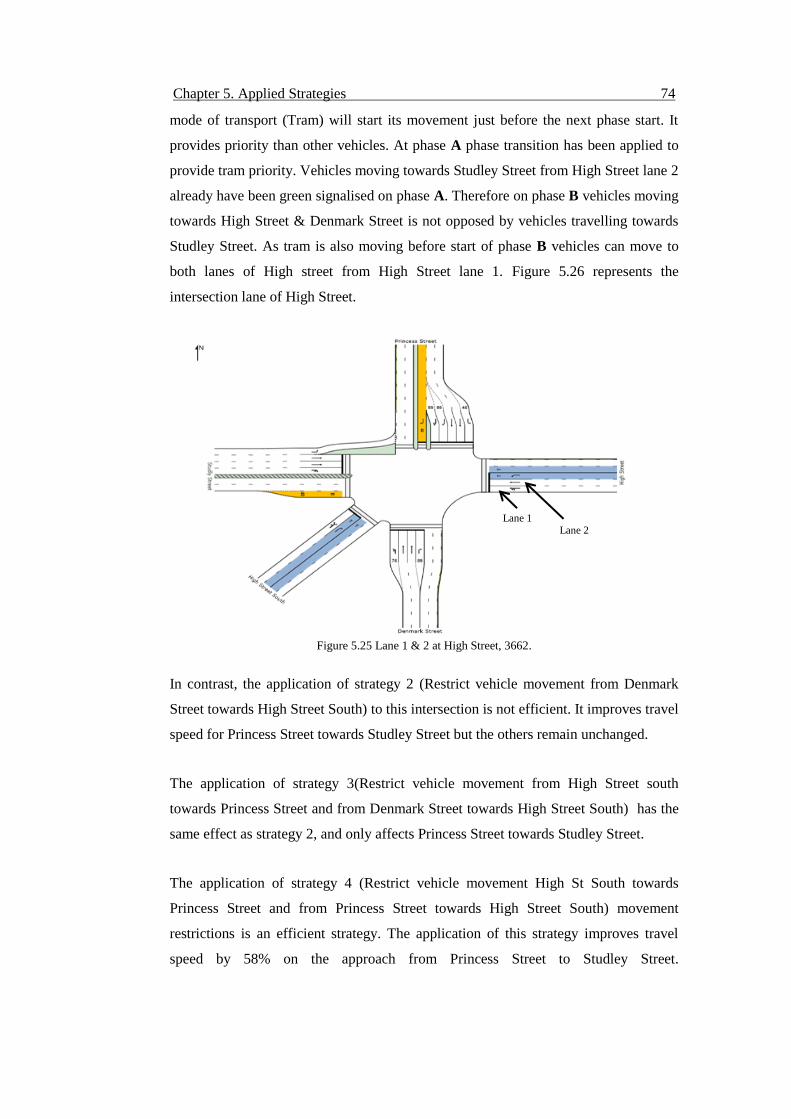
Chapter 5. Applied Strategies 74
mode of transport (Tram) will start its movement just before the next phase start. It
provides priority than other vehicles. At phase A phase transition has been applied to
provide tram priority. Vehicles moving towards Studley Street from High Street lane 2
already have been green signalised on phase A. Therefore on phase B vehicles moving
towards High Street & Denmark Street is not opposed by vehicles travelling towards
Studley Street. As tram is also moving before start of phase B vehicles can move to
both lanes of High street from High Street lane 1. Figure 5.26 represents the
intersection lane of High Street.
Figure 5.25 Lane 1 & 2 at High Street, 3662.
In contrast, the application of strategy 2 (Restrict vehicle movement from Denmark
Street towards High Street South) to this intersection is not efficient. It improves travel
speed for Princess Street towards Studley Street but the others remain unchanged.
The application of strategy 3(Restrict vehicle movement from High Street south
towards Princess Street and from Denmark Street towards High Street South) has the
same effect as strategy 2, and only affects Princess Street towards Studley Street.
The application of strategy 4 (Restrict vehicle movement High St South towards
Princess Street and from Princess Street towards High Street South) movement
restrictions is an efficient strategy. The application of this strategy improves travel
speed by 58% on the approach from Princess Street to Studley Street.
Lane 1 Lane 2
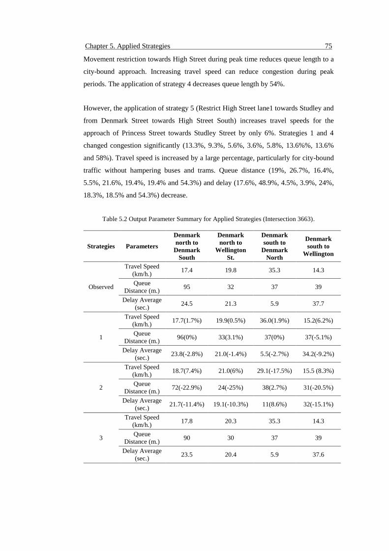
Chapter 5. Applied Strategies 75
Movement restriction towards High Street during peak time reduces queue length to a
city-bound approach. Increasing travel speed can reduce congestion during peak
periods. The application of strategy 4 decreases queue length by 54%.
However, the application of strategy 5 (Restrict High Street lane1 towards Studley and
from Denmark Street towards High Street South) increases travel speeds for the
approach of Princess Street towards Studley Street by only 6%. Strategies 1 and 4
changed congestion significantly (13.3%, 9.3%, 5.6%, 3.6%, 5.8%, 13.6%%, 13.6%
and 58%). Travel speed is increased by a large percentage, particularly for city-bound
traffic without hampering buses and trams. Queue distance (19%, 26.7%, 16.4%,
5.5%, 21.6%, 19.4%, 19.4% and 54.3%) and delay (17.6%, 48.9%, 4.5%, 3.9%, 24%,
18.3%, 18.5% and 54.3%) decrease.
Table 5.2 Output Parameter Summary for Applied Strategies (Intersection 3663).
Strategies Parameters
Denmark
north to
Denmark
South
Denmark
north to
Wellington
St.
Denmark
south to
Denmark
North
Denmark
south to
Wellington
Observed
Travel Speed
(km/h.) 17.4 19.8 35.3 14.3
Queue
Distance (m.) 95 32 37 39
Delay Average
(sec.) 24.5 21.3 5.9 37.7
1
Travel Speed
(km/h.) 17.7(1.7%) 19.9(0.5%) 36.0(1.9%) 15.2(6.2%)
Queue
Distance (m.) 96(0%) 33(3.1%) 37(0%) 37(-5.1%)
Delay Average
(sec.) 23.8(-2.8%) 21.0(-1.4%) 5.5(-2.7%) 34.2(-9.2%)
2
Travel Speed
(km/h.) 18.7(7.4%) 21.0(6%) 29.1(-17.5%) 15.5 (8.3%)
Queue
Distance (m.) 72(-22.9%) 24(-25%) 38(2.7%) 31(-20.5%)
Delay Average
(sec.) 21.7(-11.4%) 19.1(-10.3%) 11(8.6%) 32(-15.1%)
3
Travel Speed
(km/h.) 17.8 20.3 35.3 14.3
Queue
Distance (m.) 90 30 37 39
Delay Average
(sec.) 23.5 20.4 5.9 37.6
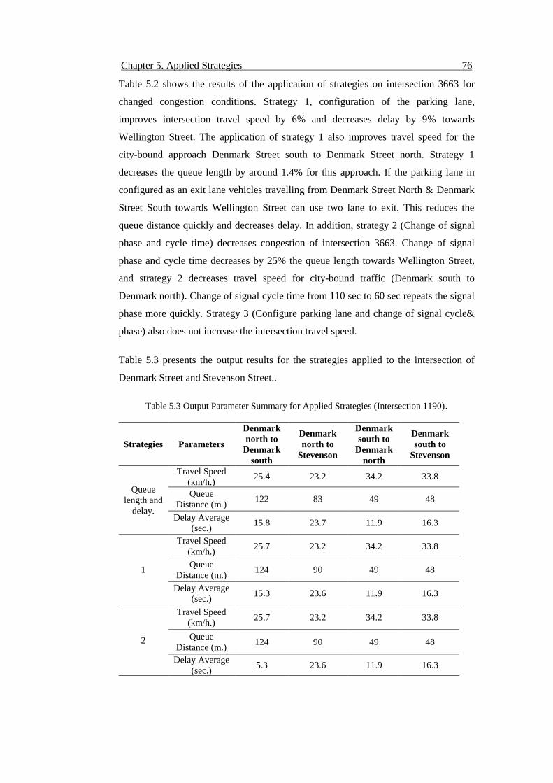
Chapter 5. Applied Strategies 76
Table 5.2 shows the results of the application of strategies on intersection 3663 for
changed congestion conditions. Strategy 1, configuration of the parking lane,
improves intersection travel speed by 6% and decreases delay by 9% towards
Wellington Street. The application of strategy 1 also improves travel speed for the
city-bound approach Denmark Street south to Denmark Street north. Strategy 1
decreases the queue length by around 1.4% for this approach. If the parking lane in
configured as an exit lane vehicles travelling from Denmark Street North & Denmark
Street South towards Wellington Street can use two lane to exit. This reduces the
queue distance quickly and decreases delay. In addition, strategy 2 (Change of signal
phase and cycle time) decreases congestion of intersection 3663. Change of signal
phase and cycle time decreases by 25% the queue length towards Wellington Street,
and strategy 2 decreases travel speed for city-bound traffic (Denmark south to
Denmark north). Change of signal cycle time from 110 sec to 60 sec repeats the signal
phase more quickly. Strategy 3 (Configure parking lane and change of signal cycle&
phase) also does not increase the intersection travel speed.
Table 5.3 presents the output results for the strategies applied to the intersection of
Denmark Street and Stevenson Street..
Table 5.3 Output Parameter Summary for Applied Strategies (Intersection 1190).
Strategies Parameters
Denmark
north to
Denmark
south
Denmark
north to
Stevenson
Denmark
south to
Denmark
north
Denmark
south to
Stevenson
Queue
length and
delay.
Travel Speed
(km/h.) 25.4 23.2 34.2 33.8
Queue
Distance (m.) 122 83 49 48
Delay Average
(sec.) 15.8 23.7 11.9 16.3
1
Travel Speed
(km/h.) 25.7 23.2 34.2 33.8
Queue
Distance (m.) 124 90 49 48
Delay Average
(sec.) 15.3 23.6 11.9 16.3
2
Travel Speed
(km/h.) 25.7 23.2 34.2 33.8
Queue
Distance (m.) 124 90 49 48
Delay Average
(sec.) 5.3 23.6 11.9 16.3
Chapter 5. Applied Strategies 77
The table 5.3 summarises the output results of SIDRA analysis and compares them
with actual intersection conditions. Signal phase order and cycle has been changed.
The three main parameters, travel speed, queue length and delay average are also
shown for this intersection. The intersection conditions remain similar after strategy
simulation. Table 5.3 shows that the application of strategies increases travel speed
and queue distance which is not ideal. If the travel speed increases, the intersection
will be cleared more quickly and queue distance will be shorter. However, at
intersection 1190 the queue distance increases for two approaches, and individual
approach delay remains same. Therefore, the application of these strategies to
intersection 1190 cannot control congestion.
The application of the strategies to intersection 3002 decreases the performance of the
intersection. All of these four intersections with each strategy were simulated as a
corridor to identify corridor performance. Efficient strategies are identified according
to increased travel speed and decreased queue distance & delay.
5.4 Results and Discussion
All the best individual intersection strategies are simulated with each other in a
network and the three main output parameters compared with actual corridor
conditions. The best strategies for application to this case study corridor are as
follows:
1. Modify signal phase order for intersection 3662 and the other three
intersections continue to operate according to present conditions.
2. Movement restriction from High Street south to Princess Street and from
Princess Street towards High Street south at intersection 3662 and the other
three intersections remain unchanged.
For both of the strategies applied for corridor congestion conditions improves at
intersection 3662. Intersections 3663, 1190 and 3002 remain unchanged.
Table 5.4 summarises the results for the simulated SIDRA network/corridor and the
percentage increases for applied strategy 1. This table compares SIDRA results of
three main parameter travel speed, queue distance and delay average with observed
values. The results are presented for individual approaches to intersection 3662.
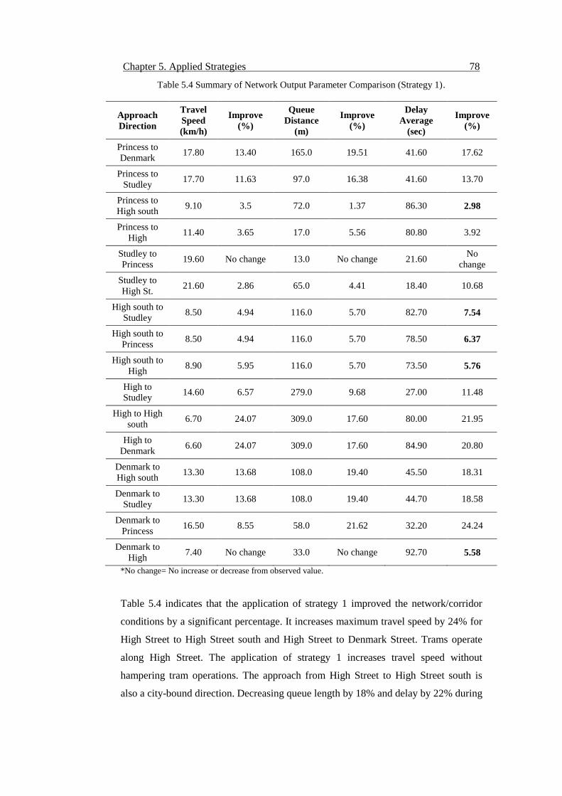
Chapter 5. Applied Strategies 78
Table 5.4 Summary of Network Output Parameter Comparison (Strategy 1).
Approach
Direction
Travel
Speed
(km/h)
Improve
(%)
Queue
Distance
(m)
Improve
(%)
Delay
Average
(sec)
Improve
(%)
Princess to
Denmark 17.80 13.40 165.0 19.51 41.60 17.62
Princess to
Studley 17.70 11.63 97.0 16.38 41.60 13.70
Princess to
High south 9.10 3.5 72.0 1.37 86.30 2.98
Princess to
High 11.40 3.65 17.0 5.56 80.80 3.92
Studley to
Princess 19.60 No change 13.0 No change 21.60
No
change
Studley to
High St. 21.60 2.86 65.0 4.41 18.40 10.68
High south to
Studley 8.50 4.94 116.0 5.70 82.70 7.54
High south to
Princess 8.50 4.94 116.0 5.70 78.50 6.37
High south to
High 8.90 5.95 116.0 5.70 73.50 5.76
High to
Studley 14.60 6.57 279.0 9.68 27.00 11.48
High to High
south 6.70 24.07 309.0 17.60 80.00 21.95
High to
Denmark 6.60 24.07 309.0 17.60 84.90 20.80
Denmark to
High south 13.30 13.68 108.0 19.40 45.50 18.31
Denmark to
Studley 13.30 13.68 108.0 19.40 44.70 18.58
Denmark to
Princess 16.50 8.55 58.0 21.62 32.20 24.24
Denmark to
High 7.40 No change 33.0 No change 92.70 5.58
*No change= No increase or decrease from observed value.
Table 5.4 indicates that the application of strategy 1 improved the network/corridor
conditions by a significant percentage. It increases maximum travel speed by 24% for
High Street to High Street south and High Street to Denmark Street. Trams operate
along High Street. The application of strategy 1 increases travel speed without
hampering tram operations. The approach from High Street to High Street south is
also a city-bound direction. Decreasing queue length by 18% and delay by 22% during
Chapter 5. Applied Strategies 79
the morning peak period has a significant effect on congestion. Less queue length
increases corridor performance and controls congestion. Traffic delay is reduced by
18% for the city-bound approach Denmark Street to High Street south. Delay is
reduced by 14% for another city-bound approach, Princess Street to Studley Street.
Table 5.5 shows the results for the simulated SIDRA network/corridor and percentage
increases for traffic conditions for strategy 2. This table compares the three main
parameters with observed values. The results are presented for individual approaches
of intersection 3662.
Table 5.5 Summary of Network Output Parameter Comparison (Strategy 2).
Approach
Direction
Travel
Speed
(km/h)
Improve
(%)
Queue
Distance
(m)
Improve
(%)
Delay
Average
(sec)
Improve
(%)
Princess to
Denmark 15.70 No change 208.00 1.50 50.50 No change
Princess to
Studley 25.30 58.12 53.00 54.31 22.00 54.36
Princess to
High south N/A N/A N/A N/A N/A N/A
Princess to
High 11.00 No change 18.00 No change 84.10 No change
Studley to
Princess 32.90 66.16 4.00 69.23 7.700 63.85
Studley to
High St 21.00 No change 68.00 No change 20.60 No change
High south to
Studley 8.30 2.47 113.00 No change 73.60 4.30
High south to
Princess N/A N/A N/A N/A N/A N/A
High south to
High 8.60 2.38 113.00 No change 67.20 3.42
High to
Studley 13.70 No change 306.00 No change 30.50 No change
High to High
south 5.40 No change 375.00 No change 102.50 No change
High to
Denmark 5.30 No change 375.00 No change 107.20 No change
Denmark to
High south 15.20 No change 134.00 No change 55.70 No change
Denmark to
Studley 11.70 No change 134.00 No change 54.90 No change
Denmark to
Princess 11.70 No change 74.00 No change 42.50 No change
Denmark to
High 7.80 No change 32.00 No change 87.50 No change
*No change= No increase or decrease from observed value.
Chapter 5. Applied Strategies 80
Table 5.5 shows the results for the application of strategy 2 to the corridor. There is a
58 % travel speed increase for the city-bound approach Princess Street to Studley
Street. The application of strategy 2 decreases queue length and delay by more than
50%. Congestion is also decreases for traffic travelling from Studley Street to Princess
Street. Queue length is reduced by 69% for this approach, indicating that applying
strategy 2 on city-bound traffic during the morning peak can control congestion.
Table 5.6 presents a summary of the simulated results for intersection 3662. The table
compares three parameters with the observed values for strategies 1 and 2.
Table 5.6 Summary of Network Output Parameter Comparison (Strategy 1&2).
Strategy
Travel
Speed
(km/h.)
Improve
(%)
Queue
Distance
(m.)
Improve
(%)
Delay
Average
(sec.)
Improve
(%)
Observed
Network 12.0 375 52.6
Applied
Strategy 1
Network
13.3 10.83 309 17.60 45.5 13.50
Applied
Strategy 2
Network
12.8 6.67 375 No Change 48.4 8.68
*No change= No increase or decrease from observed value.
Table 5.6 is numerical comparison of two strategies applied to the corridor. Both of
the strategies increase the corridor performance by increasing travel speed and
decreasing queue length and delay. The simulated corridor is mainly affected by
intersection 3662, as it is the busiest five-approach intersection, and the other three
intersections remain the same. The application of strategy 1 increases travel speed by
11 %, while strategy 2 increases travel speed by 7%. Strategy 1 improves the travel
speed by 4 % more than strategy 2. Queue length decreases by 18% using strategy 1.
In addition, travel delay also decreases by 5% through applying strategy 1 rather than
strategy 2. Strategy 1 is therefore more efficient than strategy 2 for controlling
congestion for this corridor.
Table 5.7 represents a summary of the comparison of observed and the two proposed
strategies for the whole corridor. The table clearly indicates performance improvement
for this network/corridor.
Chapter 5. Applied Strategies 81
Table 5.7 Summary of Network Output Parameter Comparison.
Output Parameter Observed
Network
Strategy 1
Network
Strategy 2
Network
Travel Speed (km/h.) 19.8 20.7 20.3
Total Travel Time (veh-h/h.) 219.8 210.0 214.1
Travel Delay (sec.) 42.0 39.3 40.4
Total Control Delay*1 (veh-
h/h.) 128.26 119.3 123.1
Congestion co-efficient*2 3.03 2.90 2.95
Total Cost ($/h.)*3 7622.7 7273.9 7447.1
*1Total control delay is the sum of delay experienced by all vehicles or pedestrians (vehicle-hours per
hour or pedestrian-hours per hour).
*2Congestion co-efficient is defined as ration of desired speed to average travel speed.
*3Total cost defines as a measure that includes the direct vehicle operating cost (the resource cost of fuel
and additional running costs including tyre, oil, repair and maintenance as a factor of the cost of fuel) as
well as the time cost of vehicle occupants.
From Table 5.7 comparisons of the two efficient strategies can be identified. The table
also shows more efficient strategies for this corridor by comparing a number of
parameters. Travel speed increases by 5% by applying strategy 1, which reduces delay
by 7%. The application of strategy 1 also reduces hourly cost by 5% for this corridor.
Strategy 2 also reduces the travel time and congestion by significant percentages,
which can help control congestion for this corridor.
5.5 Summary
Two best strategies have been identified to control congestion of this corridor. Time
priority and movement restriction are the two best strategies for this corridor. Parking
restrictions for the morning peak period on the Wellington Street intersection also
increase the LOS of this corridor. Parking restrictions on Wellington Street improve
the corridor traffic conditions but also have a minimal negative effect on Wellington
Street and Stevenson Street. As Wellington Street and Stevenson Street are less
congested parking restriction on Wellington Street during morning peak period can
consider one of the proposed strategies.
82
Chapter 6
Conclusion and Future Research
6.1 Conclusion
On the basis of computer simulations using SIDRA (30.10.2014) this thesis has
identified the potential strategies to improve the existing congestion in corridor of
Melbourne. Time priority and movement restriction are the two best strategies for this
corridor. Parking restrictions for the morning peak period at the Wellington Street
intersection also increase the LOS of this corridor, but have a minimal negative effect
on Wellington Street and Stevenson Street. The study proposes several individual
strategies which increase travel speed, decrease travel time and vehicle queue length.
For T-intersections, rearrangement of the signal phase may be effective. In addition,
for busy intersections with more than four approaches, movement restriction and lane
configuration improve the intersection and overall corridor performance.
The study proposes several individual strategies which increase travel speed and
decrease travel time. Decrease of travel time also decreases fuel consumption and cost.
Furthermore, for busy intersections with more than four approaches, movement
restriction and lane configuration improve the intersection and overall corridor
performance.
6.2 Research Contribution
The study focuses on modal congestion management as it is a more economical
solution than construction of new infrastructure and congestion pricing strategies. This
research contributes specific knowledge of strategies for modal congestion
management. The study proposes effective strategies to reduce traffic congestion for a
corridor with pedestrians and different modes of transport including trams, buses,
Chapter 6. Conclusion and Future Research 83
passenger cars and bi-cycles based on SIDRA 6 (30.10.2014) analysis. The
contributions of the present research can be summarised as follows:
The thesis models and evaluates the congestion level in a congested urban
corridor using a microscopic traffic simulation model. Previous models used
mainly mathematical models and focused on one single intersection. Using the
microscopic simulation software SIDRA this study has identified effective
strategies to control congestion. Most of the previous models described efficient
strategies based on algorithms and mathematical solutions, and the use of actual
data and corridor conditions is not common. On the basis of mathematical
solutions congestion can be controlled. However, the use of simulation software
enables the models to be observed according to practical and measured datasets.
Most previous research highlights only one intersection and simulates it. After
simulation efficient strategies can be identified. However, the present study
simulates a whole network to see the effect. This research proposes solutions to
individual intersection congestion as well as corridor congestion.
The thesis uses multi-modal strategies to control all existing modes of transport,
including passenger cars, buses, trams and bicycles. Tram networks are not
available in all cities. Simulation models for an intersection with public
transport (bus/tram), motor vehicles and pedestrians are rare. The study
suggests effective ways to control peak time traffic congestion without
obstructing public transport priority. All modes of transport are assigned signal
time as required. During the morning peak, the city-bound traffic needs more
green time to clear the intersections.
6.3 Future Research Directions
In future, research can continue to apply strategies to different intersections and
roundabouts. To control congestion using modal management strategies more
intersections can be simulated. Possible research topics are as follows:
In future, research can continue to apply strategies to different intersections and
roundabouts. To control congestion using modal management strategies more
intersections can be simulated. Possible research topics are as follows:
Chapter 6. Conclusion and Future Research 84
More intersections can be added to simulate larger corridors. As case studies,
longer corridors can be simulated. All the strategies can be applied to the new
intersections to determine the effects, particularly during peak times.
More simulated corridors could be added as a network and apply strategies to
see the effects. All effective strategies could then be applied for a large network
to control congestion could be proposed.
Signalised, un-signalised and roundabouts could be added as a network and
simulate strategies.
The corridor could be simulated during afternoon peak time. Strategies can be
applied on each intersection and corridor to identify effective strategies for the
afternoon peak time.
85
References
AASNESS, M. A. 2014. The Impact of Transforming a Road Financing Toll Scheme
to a Congestion Charging Scheme – The Case of Oslo. Transportation Research
Procedia, 1, 89-100.
ABKOWITZ, M. D. & ENGELSTEIN, I. 1983. Factors affecting running time on
transit routes. Transportation Research Part A: General, 17, 107-113.
AKCELIK, R. 1994. Estimation of green times and cycle time for vehicle actuated
signals.pdf. Transport research record, 63-72.
AKCELIK, R. 1997. Fundametal traffic varriables in adaptive controland the SCATS
DS parameter.pdf. 3rd International conference ITS Australia.
AKCELIK, R. 2007. Review of gap acceptance capacity models.pdf. 29th Conference
of Australian Institute of Transport Research.
AKCELIK, R. 2008. The relationship between drivers behaviour and capacity.pdf.
TRB National roundabout conference, Kansas City, MO, USA.
AKCELIK, R. 2012. An Improved Method for Estimating Sign-Controlled
Intersection Capacity.pdf. New Zealand Modelling User Group NZMUGS 2012
Conference. Auckland, Sep 2012.
AKÇELIK, R. & ROUPHAIL, N. M. 1993. Estimation of delays at traffic signals for
variable demand conditions. Transportation Research Part B: Methodological, 27,
109-131.
References 86
A. MEDINA, N. T., K. SALAMATIAN , S. BHATTACHARYYA, C. DIOT 2002.
Traffic Matrix Estimation: Existing Techniques and New Directions.
ANON., 1997. No room, no room. Economist 345 (8046), 21–23.
ANTIPOVA, A. & WILMOT, C. 2012. Alternative approaches for reducing
congestion in Baton Rouge, Louisiana. Journal of Transport Geography, 24, 404-410.
ARMSTRONG-WRIGHT, A. T. 1986. Road pricing and user restraint: Opportunities
and constraints in developing countries. Transportation Research Part A: General, 20,
123-127.
ARNOTT, R. & SMALL, K. 1994. The economics of traffic congestion. American
Scientist, 446-455.
BASSO, L. J., GUEVARA, C. A., GSCHWENDER, A. & FUSTER, M. 2011.
Congestion pricing, transit subsidies and dedicated bus lanes: Efficient and practical
solutions to congestion. Transport Policy, 18, 676-684.
BÖRJESSON, M., ELIASSON, J., HUGOSSON, M. B. & BRUNDELL-FREIJ, K.
2012. The Stockholm congestion charges—5 years on. Effects, acceptability and
lessons learnt. Transport Policy, 20, 1-12.
BRAY, D. J., TAYLOR, M. A. P. & SCRAFTON, D. 2011. Transport policy in
Australia—Evolution, learning and policy transfer. Transport Policy, 18, 522-532.
BUTTON, K. 2004. 1. THE RATIONALE FOR ROAD PRICING: STANDARD
THEORY AND LATEST ADVANCES. Research in Transportation Economics, 9, 3-
25.
BYUNGKYU (BRIAN) PARK, J. W., ILSOO YUN 2006. <Application of
Microscopic Simulation Model Calibration and validation.pdf>. Transportation
Research Record: Journal of the Transportation Research Board, 113-122.
CHANG, G.-L. & WU, J. 1994. Recursive estimation of time-varying origin-
destination flows from traffic counts in freeway corridors. Transportation Research
Part B: Methodological, 28, 141-160.
References 87
CHANG, G.-L., VASUDEVAN, M. & SU, C.-C. 1996. Modelling and evaluation of
adaptive bus-preemption control with and without Automatic Vehicle Location
systems. Transportation Research Part A: Policy and Practice, 30, 251-268.
CHEN, X., YU, L., ZHU, L., YU, L. & GUO, J. 2008. Microscopic Simulation
Approach to Effectiveness Analysis of Transit Signal Priority for Bus Rapid Transit:
A Case Study in Beijing. Transportation Research Record: Journal of the
Transportation Research Board, 2072, 64-76.
COLLINS, M. & WEISBROD, G. 2000. Economic Impact of Freeway Bypass Routes
in Medium Size Cities. Economic Development Research Group, Roanoke, Virginia,
1-16.
DE PALMA, A. & LINDSEY, R. 2006. Modelling and evaluation of road pricing in
Paris. Transport Policy, 13, 115-126.
DION, F. & HELLINGA, B. 2002. A rule-based real-time traffic responsive signal
control system with transit priority: application to an isolated intersection.
Transportation Research Part B: Methodological, 36, 325-343.
DOWNS, A. 2004. Traffic: Why it’s getting Worse. What Government can Do’The
Brookings Institution Policy Brief.
ELIAS, W. & SHIFTAN, Y. 2011. The safety impact of land use changes resulting
from bypass road constructions. Journal of Transport Geography, 19, 1120-1129.
ELIASSON, J. 2008. Lessons from the Stockholm congestion charging trial.
Transport Policy, 15, 395-404.
ELIASSON, J. 2009. A cost–benefit analysis of the Stockholm congestion charging
system. Transportation Research Part A: Policy and Practice, 43, 468-480.
EVANS, R. 2007. Central London congestion charging scheme-ex-post evaluation of
the quantified impacts of the original scheme.
Ferrari, P. (1989). "The effect of driver behaviour on motorway reliability."
Transportation Research Part B: Methodological 23(2): 139-150.
References 88
GENTILE, G., PAPOLA, N. & PERSIA, L. 2005. Advanced pricing and rationing
policies for large scale multimodal networks. Transportation Research Part A: Policy
and Practice, 39, 612-631.
GOH, M. 2002. Congestion management and electronic road pricing in Singapore.
Journal of Transport Geography, 10, 29-38.
GOPINATH MENON, A. & KIAN-KEONG, C. 2004. ERP IN SINGAPORE-
WHAT'S BEEN LEARNT FROM FIVE YEARS OF OPERATION? Traffic
Engineering & Control, 45.
GOUGH, C. & COOK, A. 2010. Loop detection for bus priority in MOVA SCOOT -
Notts CC come up with a cost effective solution. Traffic Engineering and Control, 51,
285-287.
GUDMUNDSSON, H., ERICSSON, E., HUGOSSON, M. B. & ROSQVIST, L. S.
2009. Framing the role of Decision Support in the case of Stockholm Congestion
Charging Trial. Transportation Research Part A: Policy and Practice, 43, 258-268.
HAMILTON, C. J. 2011. Revisiting the cost of the Stockholm congestion charging
system. Transport Policy, 18, 836-847.
HAGRING, O. 2000. Estimation of critical gaps in two major streams. Transportation
Research Part B: Methodological, 34, 293-313.
HEYNS, WERNER. "Managing Traffic Congestion–The Case of Land-Use
Management and Transport Planning Integration." Land Use Management and
Transportation Planning 86 (2015): 83.
HOUNSELL, N. B., SHRESTHA, B. P., HEAD, J. R., PALMER, S. & BOWEN, T.
2008. The way ahead for London's bus priority at traffic signals. IET Intelligent
Transport Systems, 2, 193.
JANSSON, J. O. 2010. Road pricing and parking policy. Research in Transportation
Economics, 29, 346-353.
KILANI, M., PROOST, S. & VAN DER LOO, S. 2014. Road pricing and public
transport pricing reform in Paris: Complements or substitutes? Economics of
Transportation, 3, 175-187.
References 89
KOTTENHOFF, K. & BRUNDELL FREIJ, K. 2009. The role of public transport for
feasibility and acceptability of congestion charging – The case of Stockholm.
Transportation Research Part A: Policy and Practice, 43, 297-305.
KWON, J. & VARAIYA, P. 2008. Effectiveness of California’s high occupancy
vehicle (HOV) system. Transportation Research Part C: Emerging Technologies, 16,
98-115.
LAIRD, J., NASH, C. & SHEPHERD, S. 2007. Chapter 8 Cordon charges and the use
of revenue: A case study of Edinburgh. Research in Transportation Economics, 19,
161-187.
LEAF, M. 1995. Inner city redevelopment in China: Implications for the city of
Beijing. Cities, 12, 149-162.
LEONG, D., LICHTMAN, L., MARCOS, F., MICHELSON, K. 2002. <03-
06highway291.pdf.
LI, Z. & HENSHER, D. A. 2010. Toll roads in Australia: An overview of
characteristics and accuracy of demand forecasts. Transport Reviews, 30, 541-569.
LI, Z. & HENSHER, D. A. 2012. Estimating values of travel time savings for toll
roads: Avoiding a common error. Transport Policy, 24, 60-66.
LIN, J., WANG, P. & BARNUM, D. T. 2008. A quality control framework for bus
schedule reliability. Transportation Research Part E: Logistics and Transportation
Review, 44, 1086-1098.
LITMAN, T. 2006. London congestion pricing. Implications for Other Cities.
LITMAN, T. (2012). Introduction to Multi-Modal Transportation Planning.pdf.
LIU, H., ZHANG, J. & CHENG, D. 2008. Analytical Approach to Evaluating Transit
Signal Priority. Journal of Transportation Systems Engineering and Information
Technology, 8, 48-57.
MAHROUS, R. F. (2012). Multimodal Transportation System: Modelling
Challenges.pdf.
References 90
MAY, A. D. & MILNE, D. S. 2000. Effects of alternative road pricing systems on
network performance. Transportation Research Part A: Policy and Practice, 34, 407-
436.
M. CREMER, H. K. 1986. A new class of dynamic methods for the identification of
origin-destination flows.pdf. Transport Research Board, 21B, 117-132.
MESBAH, M., SARVI, M., OUVEYSI, I. & CURRIE, G. 2011. Optimization of
transit priority in the transportation network using a decomposition methodology.
Transportation Research Part C: Emerging Technologies, 19, 363-373.
MORIYAMA, Y., MITSUHASHI, M., HIRAI, S. & OGUCHI, T. 2011. The Effect
on Lane Utilization and Traffic Capacity of Adding an Auxiliary Lane. Procedia -
Social and Behavioral Sciences, 16, 37-47.
N. B. HOUNSELL, F. N. M., E. P. SHRESTHA 2004. Bus priority at traffic signals:
Investigating the options.Pdf.
N.A.TYLER. 1991. The contribution of expert opinion to the design of high capacity
bus priority systems.pdf.
NATIONAL RESEARCH COUNCIL, T. R. B. N. A. O. S. N. R. C. T. R. B. C. O. T.,
LAND DEVELOPMENT, N. R. C. T. R. B. C. O. C. P. I. T. N. R. C. T. R. B. C. O. T.
P. P. & SYSTEMS EVALUATION, N. R. C. T. R. B. C. O. C. T. 1993. Planning and
programming, land use, public participation, and computer technology in
transportation, Washington, D.C., National Academy Press.
OGDEN, K. W. 2001. Privacy issues in electronic toll collection. Transportation
Research Part C: Emerging Technologies, 9, 123-134.
OLSZEWSKI, P. & XIE, L. 2005. Modelling the effects of road pricing on traffic in
Singapore. Transportation Research Part A: Policy and Practice, 39, 755-772.
OLSZEWSKI, P. S. 2007. Singapore motorisation restraint and its implications on
travel behaviour and urban sustainability. Transportation, 34, 319-335.
PALMA, A. D., LINDSEY, R. & PROOST, S. 2006. Research challenges in
modelling urban road pricing: An overview. Transport Policy, 13, 97-105.
References 91
PAPAGEORGIOU, M. 1990. Dynamic modeling, assignment, and route guidance in
traffic networks. Transportation Research Part B: Methodological, 24, 471-495.
PARK BYUNGKYU (BRIAN) , S. J. D. 2003. Microscopic simulation model
calibration and validation.pdf. Transportation Research Record: Journal of the
Transportation Research Board, 1856/2003, 185-192.
PARRY, I. W. H. 2002. Comparing the efficiency of alternative policies for reducing
traffic congestion. Journal of Public Economics, 85, 333-362.
QI, B. P. H. 2006. Microscopic simulation model calibration and validation for
freeway work zone network.pdf. Intelligent Transportation Systems Conference, 2006.
ITSC '06. IEEE, 1471 - 1476.
RICH, J. & NIELSEN, O. A. 2007. A socio-economic assessment of proposed road
user charging schemes in Copenhagen. Transport Policy, 14, 330-345.
SANTOS, G. & BHAKAR, J. 2006. The impact of the London congestion charging
scheme on the generalised cost of car commuters to the city of London from a value of
travel time savings perspective. Transport Policy, 13, 22-33.
SANTOS, G., LI, W. W. & KOH, W. T. H. 2004. 9. TRANSPORT POLICIES IN
SINGAPORE. Research in Transportation Economics, 9, 209-235.
SANTOS, G., et al. (2010). "Part II: Policy instruments for sustainable road transport."
Research in Transportation Economics 28(1): 46-91.
SAYED, T., BROWN, G. & NAVIN, F. 1994. Simulation of traffic conflicts at
unsignalized intersections with TSC-Sim. Accident Analysis & Prevention, 26, 593-
607.
SIDRA 2013. SIDRAINTERSECTION_UserGuide.pdf.
SMALL, K. A. & VERHOEF, E. T. 2007. The economics of urban transportation,
Routledge.
SRINIVASAN, S. & KOCKELMAN, K. 2002. The impacts of bypasses on small-and
medium-sized communities: an econometric analysis. Journal of Transportation and
Statistics, 5, 57-69.
References 92
STERMAN, B. P. & SCHOFER, J. L. 1976. Factors affecting reliability of urban bus
services. Journal of Transportation Engineering, 102.
STRATHMAN, J. G. & HOPPER, J. R. 1993. Empirical analysis of bus transit on-
time performance. Transportation Research Part A: Policy and Practice, 27, 93-100.
TIRACHINI, A., et al. (2014). "Multimodal pricing and optimal design of urban
public transport: The interplay between traffic congestion and bus crowding."
Transportation Research Part B: Methodological 61(0): 33-54.
TRANSPORT, A. (2007). <wp_071.pdf>.
TSEKERIS, T. & VOΒ, S. 2009. Design and evaluation of road pricing: state-of-the-
art and methodological advances. Netnomics, 10, 5-52.
TURNQUIST, M. A. 1978. A model for investigating the effects of service frequency
and reliability on bus passenger waiting times. Transportation Research Record.
VAN VUGT, M., VAN LANGE, P. A. & MEERTENS, R. M. 1996. Commuting by
car or public transportation? A social dilemma analysis of travel mode judgements.
European Journal of Social Psychology, 26, 373-395.
VERHETSEL, A. 2001. The impact of planning and infrastructure measures on rush
hour congestion in Antwerp, Belgium. Journal of Transport Geography, 9, 111-123.
VIEGAS, J. & LU, B. 2004. The Intermittent Bus Lane signals setting within an area.
Transportation Research Part C: Emerging Technologies, 12, 453-469.
WAHLSTEDT, J. 2011. Impacts of Bus Priority in Coordinated Traffic Signals.
Procedia - Social and Behavioral Sciences, 16, 578-587.
WANG, Y., ZHU, X., LI, L. & WU, B. 2013. Reasons and Countermeasures of
Traffic Congestion under Urban Land Redevelopment. Procedia - Social and
Behavioral Sciences, 96, 2164-2172.
XIE, L. & OLSZEWSKI, P. 2011. Modelling the effects of road pricing on traffic
using ERP traffic data. Transportation Research Part A: Policy and Practice, 45, 512-
522.
References 93
YAGAR, S. & HAN, B. 1994. A procedure for real-time signal control that considers
transit interference and priority. Transport Research Board, 28B, 315-331.
YAN, X., RADWAN, E. & GUO, D. 2007. Effects of major-road vehicle speed and
driver age and gender on left-turn gap acceptance. Accident Analysis & Prevention,
39, 843-852.
YANG, H., SASAKI, T., IIDA, Y. & ASAKURA, Y. 1992. Estimation of origin-
destination matrices from link traffic counts on congested networks. Transportation
Research Part B: Methodological, 26, 417-434.
YIN, Y., LAM, W. H. & MILLER, M. A. 2004. A simulation‐based reliability
assessment approach for congested transit network. Journal of advanced
transportation, 38, 27-44.
94
Appendix A
VicRoads Data
For analysing corridor the traffic volumes for one hour morning peak period traffic
has been used. A normal working day has been chosen for this simulation.
Table A1 shows the summary of traffic volumes from 7.30 am to 8.30 am. Traffic
volumes were calculating using detectors. Total mode of transport passing through
detectors is the traffic volume. Bus/tram are counted as heavy vehicle and calculated
as 2.5 times of passenger cars (SIDRA 2013). Total vehicle travelling on lane has been
collected from VicRoads datasets. In some cases (approaches vehicles are moving
more than one direction (Through/left/right) from one lane. Traffic volume has been
calculated for such cases by using percentage of vehicle turning to direction
(left/right/through). Through survey the percentage of vehicle turning has been
identified. From survey how many vehicle moving towards left/right or through
direction has been calculated. The percentage of vehicle moving towards more than
one direction from a single lane is mentioned on Table A2.
Table A2 presents a summary of all the intersection geometries, including lane
numbers, types of vehicle movement, and percentages of vehicle movement in a
particular direction. The table also summarises the parking lane and bicycle lane
restrictions for one morning peak hour. The lane width is 4.2m and the cycle lane
width is 0 .50m.
Table A1 Summary of Traffic Volumes.*
Intersection Name Approach Name Traffic Volume (7.30 am to 8.30 am)
Princess Street/Studley
Street/High Street South/
Denmark Street/ High
Street
To Princess To Studley To High South To Denmark To High
Princess Street N/A 329 125 855 33
Studley Street 53 N/A 1 1 530
High Street South 79 48 N/A N/A 117
Denmark Street 356 174 116 N/A 58
High Street N/A 834 384 200 N/A
Denmark Street/
Wellington Street
To Denmark (Through) To Wellington To Denmark (Left
turn)
To Denmark
(Right Turn)
Denmark Street(South) 602 147 N/A N/A
Denmark Street(North) 791 170 N/A N/A
Wellington Street N/A N/A 228 150
Denmark Street/
Stevenson Street
To Denmark (Through) To Stevenson To Denmark
(Left turn)
To Denmark
(Right Turn)
Denmark Street (South) 676 64 N/A N/A
Denmark (North) 1005 150 N/A N/A
Stevenson Street N/A N/A 30 33
Denmark Street/ Power
Street/ Barkers Road
To Power To Denmark To Barkers To Barkers
(Left)
To Barkers
(Right)
Denmark Street 739 N/A N/A 100 298
Power Street N/A 538 N/A 77 298
Barkers Road (West) 73 100 467 N/A N/A
Barker Road (East) 133 133 983 N/A N/A
*VicRoads SCATS Data.
95
96
Table A2 Summary of Intersection Geometries and Movements.*
Site
Name
Approach
Name(ST)
Lane
No(T)
Right Turn
Lane No
Left Turn
Lane No
Sleep /Dedicated
Lane
% of Vehicle
Movement
Speed,
Km/h
Movement
Restriction,
Peak period
Parking
Restriction, Peak
period
3662
Princess 2 2,1- to
Studley,1-
High South,
Short L
1 1 Dedicated bus
lane
57% to High South 60 None Yes
Studley 2 1-High South None 1 Sleep lane N/A 60 Right turn Yes
High
South
2 Restricted 1-Studley,
Princess St,1-
High St
1 tram lane shared
with other traffic
20% High, 30%
Studley,50%
Princess,
40 Right turn
always
Yes
Denmark 2 1, Short lane 1-High St
South, Studley
St, Short lane
None 40% High
South,60% Studley
60 None Yes
High 2 Restricted 2,1-Denmark,
1-High South
Dedicated Tram
Lane
27% Denmark,21%
Studley
40 Right Turn
always
Yes
3663 Denmark 2 1 short lane Shared left None 33% Wellington 60 None Yes
Wellington None 1 1 None N/A 60 None Exit direction
1190 Denmark 2 Shared Right N/A None 44%to L, 30% to R 60 No
Stevenson 1 Shared Right Shared left 49% L, 51% R 60 No
3002
Denmark 2 1-Short lane Shared lane None 24% to Barker 60 None Yes
Power 2 1, Short lane Shared Left
lane
None 34% to Barker 60 None Yes
Barkers 2 1, Short lane 1 Sleep lane to left 50% to Denmark 60 None Yes
* Survey.
97
APPENDIX B
MOVEMENT SUMMARY
Movement summary output results for each intersection have been presented. The
summary results are for vehicles travelling through each intersection and each
direction. The resultant table presents movement Id, OD movement, total vehicle/hour,
Demand flow for heavy vehicle, degree of saturation, average delay, level of service,
95% back of queue vehicles ,distance, proportion queued, effective stop rate per
vehicle and average speed.
Table B1 shows the output movement summary of intersection Denmark Street, High
Street, Studley Street, Princess Street and High Street south.
Table B2 represents the output movement summary of intersection Denmark Street
and Wellington Street.
Table B3 represents the output movement summary of intersection Denmark Street
and Stevenson Street.
Table B4 shows the output movement summary of intersection Power Street, Barker
Road and Denmark Street.
98
Table B1 Output Movement Summary of intersection Denmark Street, High Street, Studley Street, Princess Street and High Street south.
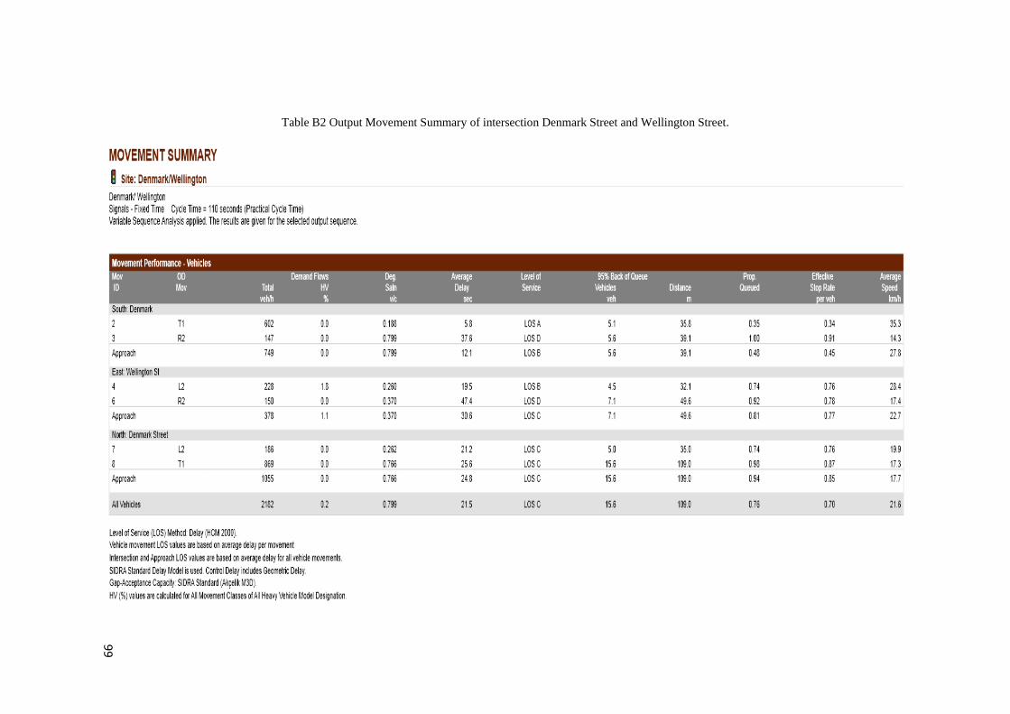
99
Table B2 Output Movement Summary of intersection Denmark Street and Wellington Street.
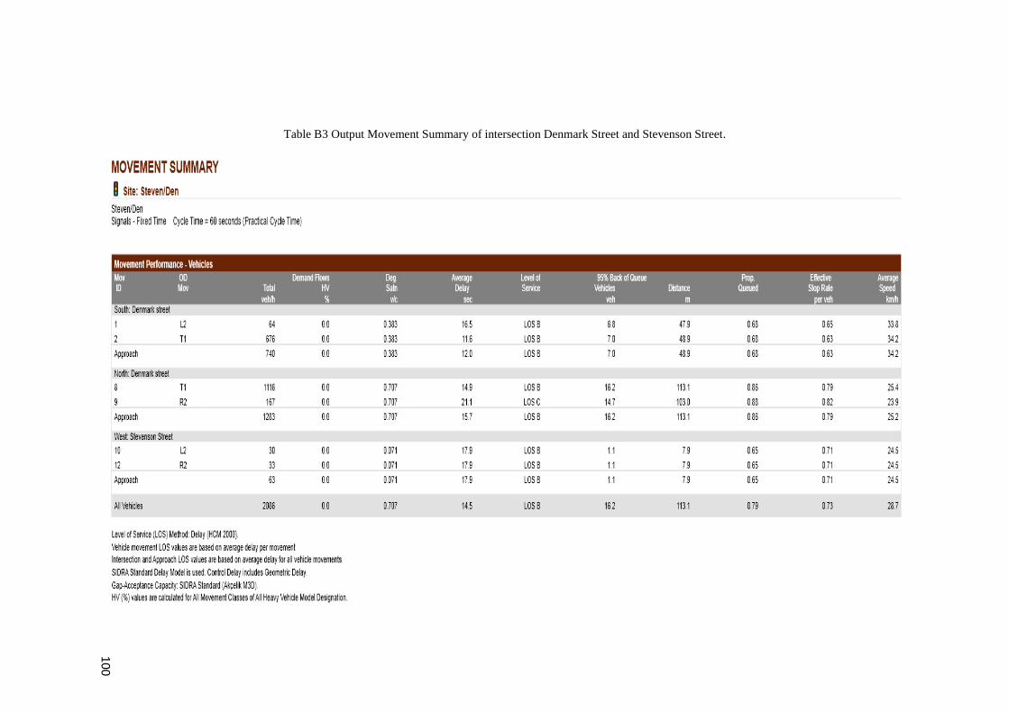
100
Table B3 Output Movement Summary of intersection Denmark Street and Stevenson Street.
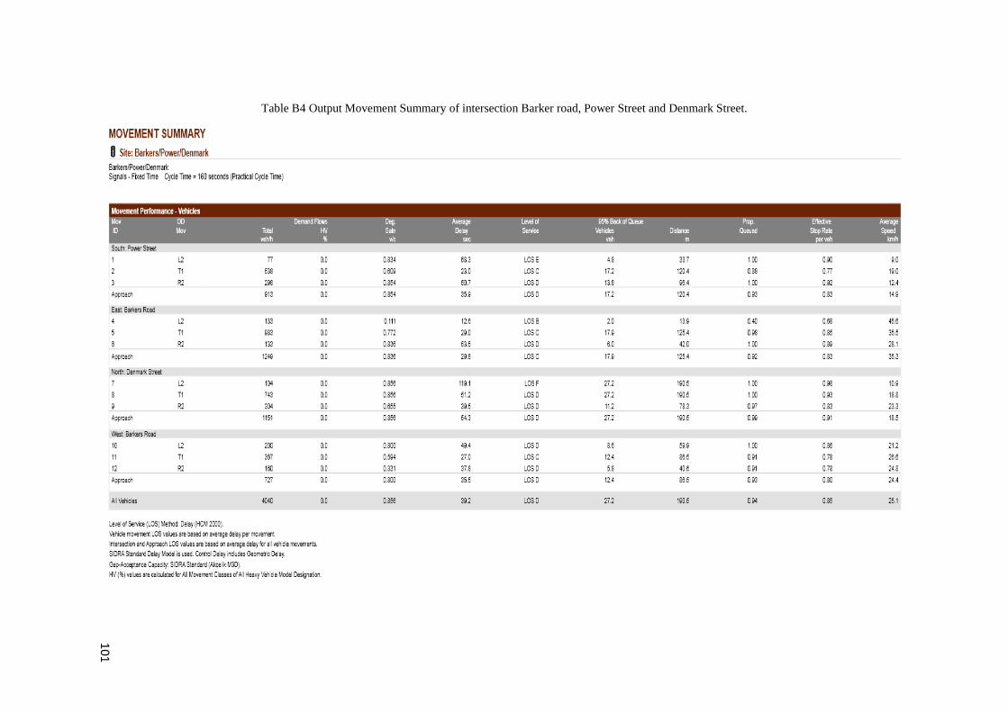
101
Table B4 Output Movement Summary of intersection Barker road, Power Street and Denmark Street.