Modal Based Tanpura Simulation: Combining Tension

Modal Based Tanpura Simulation: Combining Tension Modulation andDistributed Bridge Interaction

Bridges, J., & Van Walstijn, M. (2017). Modal Based Tanpura Simulation: Combining Tension Modulation andDistributed Bridge Interaction. In Proceedings of the 20th International Conference on Digital Audio Effects(DAFx-17 (pp. 299-306). (Proceedings of the International Conference on Digital Audio Effects)..http://www.dafx17.eca.ed.ac.uk/papers/DAFx17_paper_67.pdf

Published in:Proceedings of the 20th International Conference on Digital Audio Effects (DAFx-17

Document Version:Publisher's PDF, also known as Version of record

Queen's University Belfast - Research Portal:Link to publication record in Queen's University Belfast Research Portal

Publisher rights© 2017 The Authors.Published in the Proceedings of the 20th International Conference on Digital Audio Effects (DAFx-15). This work is made available online inaccordance with the publisher’s policies. Please refer to any applicable terms of use of the publisher.

General rightsCopyright for the publications made accessible via the Queen's University Belfast Research Portal is retained by the author(s) and / or othercopyright owners and it is a condition of accessing these publications that users recognise and abide by the legal requirements associatedwith these rights.

Take down policyThe Research Portal is Queen's institutional repository that provides access to Queen's research output. Every effort has been made toensure that content in the Research Portal does not infringe any person's rights, or applicable UK laws. If you discover content in theResearch Portal that you believe breaches copyright or violates any law, please contact [email protected].

Download date:26. Jan. 2022

http://www.dafx17.eca.ed.ac.uk/papers/DAFx17_paper_67.pdf

https://pure.qub.ac.uk/en/publications/modal-based-tanpura-simulation-combining-tension-modulation-and-distributed-bridge-interaction(9a5e83e7-f0f7-40b4-be91-5af550f38343).html

Proceedings of the 20th International Conference on Digital Audio Effects (DAFx-17), Edinburgh, UK, September 5–9, 2017

MODAL BASED TANPURA SIMULATION: COMBINING TENSION MODULATION ANDDISTRIBUTED BRIDGE INTERACTION

Jamie Bridges, Maarten Van Walstijn

Sonic Arts Research Centre

School of Electronics, Electrical Engineering, and Computer Science

Queen’s University Belfast, UK

jbridges05,[email protected]

ABSTRACT

Techniques for the simulation of the tanpura have advanced sig-

nificantly in recent years allowing numerically stable inclusion of

bridge contact. In this paper tension modulation is added to a tan-

pura model containing a stiff lossy string, distributed bridge con-

tact and the thread. The model is proven to be unconditionally

stable and the numerical solver used has a unique solution as a

result of choices made in the discretisation process. Effects due

to the distribution of the bridge contact forces by comparison to a

single point bridge and of introducing the tension modulation are

studied in simulations. This model is intended for use in furthering

the understanding of the physics of the tanpura and for informing

the development of algorithms for sound synthesis of the tanpura

and similar stringed instruments.

1. INTRODUCTION

The tanpura is an Indian stringed instrument known for its dis-

tinctive droning sound which features a time-dependent formant

of frequencies referred to as the "jvari". The generation of the

jvari depends heavily on the interaction between the strings and

the bridge over which they pass. The jvari also relies strongly on

the position of a thread which is placed between each string and

the bridge. This changes how much of the string can interact with

the bridge and only when placed within a certain range of positions

will the tanpura produce the jvari [1]. The sound of the jvari can

be altered by moving the thread within the range.

The interaction between barriers and strings is not unique to

this instrument; models of the guitar [2], violin [3] and many oth-

ers have been developed which include this phenomenon. The

non-analytic nature of contact forces requires some care to be taken

to ensure that any model including them will be stable. Energy

methods proved to be an effective way to maintain stability [4, 5, 6]

by ensuring that the numerical energy or some analogous quantity

is conserved for all time steps when there are no energy losses or

gains from external factors. Within the umbrella of energy meth-

ods there are differing approaches to creating models; differentia-

tion in time can be carried out with different approximations giving

a temporal second order form [7] or a temporal first order form [5].

Models of stringed instruments have made use of finite difference

methods [8, 5] as well as modal based methods [9]. The latter al-

low completely eliminating numerical dispersion by exactly fixing

the modal frequencies and damping which removes mode detuning

[9]. This is particularly important in the case of the tanpura as the

jvari is sensitive to any numerical warping of the partial structure.

In addition to unconditional stability it is possible to ensure that

the numerical solver has a unique solution [9] which in conjunc-

Figure 1: A simplified sketch of the tanpura model with the thread

and bridge zoomed in on significantly.

tion with the stability allows the model to be run at standard audio

sampling frequencies and maintain global trends.

In this paper tension modulation and a distributed bridge are

included in a model of the tanpura. A sketch of the model is shown

in Figure 1. Both of these effects have been modelled in musical

acoustics before but they have not yet been brought together in a

tanpura model. Tension modulation has been recently considered

in the modelling of Portugese twelve string guitars [10], the guitar

[2] and more in depth for the general case [11]. However, none

of these treatments have all of the desired attributes of having a

modal basis, uniqueness of the iterative solver solution and prov-

able stability. As this is the case a new formulation is developed

here which brings all of these aspects together. The effect of the

tension modulation in a string becomes particularly relevant when

strings have a low tension (as they tend to on a tanpura) and/or a

high Young’s modulus and cross sectional radius. The manner in

which tension modulation was included will be more discussed in

more detail in Section 2.5.

The tanpura’s bridge has traditionally been described as a two

point bridge, meaning that the string is assumed to terminate at the

thread and interacts at only one point on the bridge [12]. A recent

paper written by Issanchou et al. [13] demonstrates an impres-

sive agreement between experiments and a time-domain model for

a two point bridge system, which is an important step in the val-

idation of models which include non linear contact. This result

was found for a high tension of 180.5N and using a guitar string

whereas a more common tension for a tanpura string is between

30N and 40N. Hence questions remain regarding as to whether

there is a difference between distributed bridge and point bridge

interaction at lower tensions and what difference it would make

to the jvari. An approach similar to that in [14] here is devel-

oped which involves not treating the thread as an end point but

as a damper. Following techniques used there the thread and the

plucking signal are modelled as single point forces but with a small

spatial distribution associated with them. The incorporation of the

distributed bridge is outlined in Section 2.7.

DAFX-299

http://http://www.sarc.qub.ac.uk


2. METHOD

2.1. Overview

The Newtonian form of the equation which describes the desired

system in terms of the string’s vertical displacement y(x, t) (writ-

ten as y for brevity), horizontal position x and time t can be written

ρA∂2y

∂t2= T0

∂2y

∂x2−EI

∂4y

∂x4−γ

∂y

∂t+Ftm +Fc +Fb +Fe, (1)

where ρ represents the mass density, A the cross sectional area, Ethe Young’s modulus, I the moment of inertia and T0 the resting

tension of the string. γ gives the effect of frequency dependent

damping and will be defined later. The F terms on the right-hand

side of the equation represent additional force densities which act

on the string. Respectively these are due to tension modulation

(Ftm), the cotton thread (Fc), the bridge (Fb) and the excitation

(Fe). All of these are functions of both x and t and are defined

over the length of the string (L), although some of them only have

an effect over a small range of x. The string is assumed to be

simply supported for the boundary conditions.

2.2. Modal version

In order to eliminate numerical dispersion a modal framework is

used. This involves using the equation

y(x, t) =

M∑

i=1

vi(x)yi(t), (2)

where yi(t) are the modal displacements, vi(x) = sin(βix) are

the modal shapes and βi =iπL

. For this to be a perfect representa-

tion of the string the number of modes (M ) would be infinity.

After substituting equation (3) into (1) and integrating spa-

tially over the string the following equation is found which de-

scribes the dynamics of a single mode

m∂2yi(t)

∂t2= −kiyi(t)− ri

∂yi(t)

∂t+

∑

ǫ

Fǫ,i(t), (3)

where m = ρAL2

, ki = L2(T0β

2i + EIβ4

i ), ri = L2γ(βi) and

ǫ = tm, c, b, e. γ(βi) is now expressed as

γ(βi) = 2ρA[

σ0 + (σ1 + σ3β2i )|βi|

]

. (4)

σ0, σ1 and σ3 shape the frequency dependence to match to a real

string as closely as possible [14]. Fǫ,i, the modal driving forces,

are derived in different ways according to how the physical effect

being considered is modelled. Each one will be explained in its

relevant section.

Equation (1) can be rewritten in first-order form, which is ex-

actly equivalent, to read

∂yi(t)

∂t=pi(t)

m(5)

∂pi(t)

∂t= −kiyi(t)− ri

∂yi(t)

∂t+

∑

ǫ

Fǫ,i(t) (6)

Where pi(t) is the momentum equivalent of the ith mode.

2.3. Single forces of fixed spatial distribution

Some of the force densities will be represented as a single-variable

force term which is assumed to be spatially applied to the string

according to a fixed distribution function. This is affected by ex-

pressing the force densities as the force (Fz(t)) multiplied by a

spatial distribution function in the following fashion

Fz(x, t) = ψz(x)Fz(t), (7)

where the spatial distribution ψz(x) is defined as

ψz(x) =π

2wz

cos

[

π

wz

(x− xz)

]

, (8)

inside the domain [xz −12wz, xz +

12wz] and 0 otherwise [14]. wz

is the width of the spatial distribution and xz the central point. The

forces concerned will depend on the averaged string displacement

at the point xz, which can be written as

yz(t) =

∫ xz+wz/2

xz−wz/2

ψz(x)y(x, t)dx (9)

Evaluating equation (9) and converting to the modal form, the fol-

lowing equations can be found

Fz,i(t) = gz,iFz(t), (10)

and

yz(t) =

M∑

i=1

gz,iyi(t), (11)

where

gz,i =π2 sin(βixz) cos(

βiwz

2)

π2 − βi2wz

2. (12)

2.4. Discretisation in time

To solve equations (5) and (6) the following discretisation opera-

tors are used to find the system dynamics

δφ(t) = φn+1 − φn ≈ ∆t∂φ(t)

∂t

∣

∣

∣

∣

t=(n+ 1

2)∆t

(13)

µφ(t) = φn+1 + φn ≈ 2φ|t=(n+ 1

2)∆t, (14)

using ∆t = 1/fs. When discretising equations (5) and (6) it is

more compact to use the substitution qni = ∆t2mpni to give the equa-

tions

δyn+ 1

2

i = µqn+ 1

2

i (15)

δqn+ 1

2

i = −aiµyn+ 1

2

i − biδyn+ 1

2

i + ξ∑

ǫ

Fn+ 1

2

ǫ,i (16)

at the temporal mid point. The constants are defined as ξ =∆t2/(2m), ai = ki∆t

2/(4m) and bi = ri∆t/(2m). The in-

dividual cases of Fn+ 1

2

ǫ,i will be explained in their relevant section.

To correct for numerical dispersion ai and bi are replaced by a∗iand b∗i ; this enforces exact modal frequencies and damping for

each mode [14]. The corrected parameters read

a∗i =1− 2RiΩi +R2

i

1 + 2RiΩi +R2i

and b∗i =2(1−R2

i )

1 + 2RiΩi +R2i

, (17)

DAFX-300


where Ri = exp(−αi∆t) and Ωi = cos(ωi∆t).To solve equations (15) and (16) computationally they are rewrit-

ten as vectors in the following form:

δyn+ 1

2 = µqn+ 1

2 (18)

δqn+ 1

2 = −Aµyn+ 1

2 −Bδyn+ 1

2 + ξ∑

ǫ

Fn+ 1

2

ǫ,i (19)

In these equations Aii = a∗i and Bii = b∗i with all off-diagonal

elements in both matrices being zero. Using the same procedure

taken in previous papers [14] of setting s = δyn+ 1

2 = µqn+ 1

2

and then using the relations:

yn+1 = s+ y

nand q

n+1 = s− qn, (20)

equation (19) can be re-written as:

G = (I+A+B)s− 2(qn −Ayn)− ξ

∑

ǫ

Fn+ 1

2

ǫ,i = 0, (21)

Once the tension modulation, bridge, thread and input modal forces

are discretised properly and put into this equation it can be solved

iteratively using Newton’s method. The Jacobian required for this

is

J = Js − ξ∑

ǫ

Jǫ, (22)

where

Js = I+A+B, (23)

and Jǫ are the parts of the Jacobian due to the other forces. All of

the parts of the Jacobian will be derived below.

To prevent spectral fold over in the model the number of modes

(M) must be limited, setting the sizes of y and q, so that the fre-

quency of the highest partial is below the Nyquist frequency set by

the sampling frequency.

2.5. Tension modulation

2.5.1. Continuous domain

The force density present in the string due to tension modulation

is represented in the following equation

Ftm(x, t) =EA

2L

∫ L

0

(

∂y

∂x

)2

dx∂2y

∂x2. (24)

Following the procedure for converting to the modal domain this

can be rewritten as

Ftm(x, t) = −EA

4

[

M∑

i=1

yi(t)vi(x)β2i

][

M∑

j=1

(βj yj(t))2

]

. (25)

This is found using the orthogonal nature of the sinusoidal basis

set within the integral. From this the desired modal force can be

derived by multiplying with the modal shape and integrating over

the string giving

Ftm,i(t) = −Γyi(t)β2i

[

M∑

j=1

(βj yj(t))2

]

, (26)

where Γ = EAL8

. This equation shows how the modes are mixed,

with tension modulation having the effect of diffusing energy be-

tween modes. This is then rewritten in vector form to give:

Ftm = −Γ(β2y)y⊺β2y. (27)

Where β2 is a diagonal M × M matrix with entries along the

diagonal of β2i .

2.5.2. Discretisation of tension modulation equation in time

Equation (27) can be discretised in three ways and equation (28)

shows the option that is used. This choice was made as it preserves

the uniqueness of the solution to the iterative solver, this will be

proven in Section 3.1.

Fn+ 1

2

tm = −Γ

4(µ(y⊺β2y))β2µy. (28)

After the discretisation operator is applied and using equation (20)

the following equation is obtained

Ftm(s) = −Γ

4((yn+ s)⊺β2(y

n+ s)+(yn)⊺β2yn)β2(2y

n+ s).

(29)

This can then be inserted into equation (21). For ease of differen-

tiation (29) is rewritten as

Ftm(s) = −Γ

4(α2(s)U(s) + α1U(s)), (30)

where

U(s) = β2(2yn + s) (31)

α2(s) = (yn + s)⊺β2(yn + s) (32)

α1 = (yn)⊺β2yn

(33)

To differentiate α2(s) with respect to s the vector calculus rule:

∂g(x)⊺Ch(x)

∂x= g(x)⊺C

∂h(x)

∂x+ h(x)⊺C⊺ ∂g(x)

∂x, (34)

is used. In the equation being considered β2 which corresponds to

C is diagonal so it is equal to its own transpose. This gives:

∂α2(s)

∂x= 2(s+ y

n)⊺β2. (35)

Differentiating U(s) with respect to s gives

∂U(s)

∂s= β2. (36)

Then using the product rule the Jacobian of the tension modulation

part of the G function can be written as

Jtm(s) = −Γ

4(α2β2 +U(s)

(

2(s+ 2yn)⊺β2

)

+ α1β2). (37)

As Jtm is a full matrix the addition of the tension modulation sig-

nificantly increases computational time due to the linear system

solving required in each iteration.

It has been shown by Bilbao [8] that, using a similar modal

formulation, significant pitch glide in the wrong direction can arise

due to tension modulation if the number of modes used creates

partials up to the Nyquist frequency. However it was found that

this spurious effect could not be replicated in the model even for

extreme amplitudes.

2.6. Thread

2.6.1. Continuous domain

In the model the thread is treated as described in Section 2.3. The

equation for the force is

Fc(t) = Kc(hc − yc(t))−Rc

∂yc(t)

∂t, (38)

DAFX-301


where Kc is the spring stiffness of the thread, yc is the vertical

displacement of the string at the thread point, t is the time, hc

is the thread equilibrium point and Rc is the thread loss parame-

ter. hc was set to zero for all modelling purposes and as such will

be omitted in the following equations. When re-expressed in the

modal domain this equation reads

Fc,i(t) = −gc,i

M∑

i=1

gc,i

(

Kcyi(t) +Rc

∂yi(t)

∂t

)

. (39)

2.6.2. Discretisation of thread equation in time

Using the discretisation operators on the force function and the

equation yn+1i = si + yni the equation for the modal force at time

step n+ 12

can be written

Fn+ 1

2

c = −gcg⊺

c

(

Kc

2(s+ 2yn) +

Rc

∆ts

)

, (40)

in vector form. To solve for s the Jacobian of this vector is re-

quired. This is:

Jc = −

(

Kc

2+Rc

∆t

)

gcg⊺

c . (41)

2.7. Distributed Barrier

2.7.1. Continuous domain and spatial discretisation

To model the bridge a contact law is used to simulate the compres-

sion of the string and barrier. The contact law used is

Fb(x, t) = kb⌊hb(x)− y(x, t)⌋α, (42)

where kb is the barrier stiffness per unit length, hb(x) is the height

of the bridge at position x and α is the exponent that governs the

bridge interaction. Following [14] the exponent is set according to

Hertzian theory as α = 1 and the formulation is carried out with

this in place. Other choices of α ≥ 1 are possible and all of the

terms required for solving related to the bridge can be derived in

this general case. The force density and the string displacement in

this equation are defined over [xb −12ωb, xb +

12ωb] which is the

spatial domain of the bridge; the force density will be zero outside

this region. The potential energy density for the bridge will also

be required

Vb(x, t) =kb

2⌊hb(x)− y(xb, t)⌋

2, (43)

as will another definition for the force

Fb(x, t) = −∂Vb

∂y. (44)

For use in equation (21) the modal force vector Fb must be

found. This would usually be done by integrating over the length

of the string as follows

Fb,i(t) =

∫ L

0

vi(x)Fb(x, t)dx, (45)

but due to the non-analytic nature of Fb(x, t) it is approximated as

a Riemann sum [9]

Fb,i(x, t) ≈

K∑

k=1

vi,kFb,k(xk, t)∆x. (46)

The bridge is defined to have K points along its length, vi,k gives

each modal amplitude at the spatial position k in the domain of the

barrier and Fb,k(xk, t) is the contact force density at point k and

time t.

2.7.2. Discretisation of bridge equation in time

Writing the potential density at time step n gives

Vnb,k(t) =

kb

2⌊hb,k − ynk ⌋

2, (47)

here ynk is at the corresponding bridge point to hb,k in each case.

Equation (44) is discretised in time to give

Fn+ 1

2

b,k = −Vn+1

b,k − Vnb,k

yn+1k − ynk

. (48)

These equations are combined to give

Fn+ 1

2

b,k = −kb

2

⌊hb,k − (sk + ynk )⌋2 − ⌊hb,k − ynk ⌋

2

sk. (49)

Where again sk is at the corresponding barrier point to hb,k. Fol-

lowing from equation (49) and vectorising gives the equation

Fn+ 1

2

b = ∆xV⊺F

n+ 1

2

b , (50)

where V is a K ×M matrix which holds all of the modal shapes

at each point along the bridge. Fn+ 1

2

b must be differentiated with

respect to s for use in Newton’s method so this is done by using

the chain rule, giving the Jacobian for the barrier as

Jb = ∆xV⊺ ∂F

n+ 1

2

b

∂s

∂s

∂s, (51)

where

y = Vy and s = Vs. (52)

Obviously ∂s∂s

= V. Explicitly Jb is written as

Jb =kb∆x

2V

⊺ζV, (53)

where ζ is a diagonal matrix with the dimensions K × K. The

diagonal entries in the matrix range from ζ1,1 which is the closest

bridge point to the thread to ζK,K which is the furthest bridge point

from the thread are:

ζk,k =⌊hb,k − (sk + ynk )⌋

2 − ⌊hb,k − ynk ⌋2

s2k−2⌊hb,k − (sk + ynk )⌋

sk.

(54)

2.7.3. Single point bridge

For comparison the distributed bridge was made replaceable by a

single point bridge in the model. The single force bridge has a

different equation for the force density which is

Fb(x, t) = δ(x− xb)kb⌊hb(x)− y(x, t)⌋, (55)

xb here is the spatial position of the bridge point. When this is put

into equation (45) the integral becomes exactly solvable and gives

a modal force for mode i of

Fb,i(t) = vi(xb)kb⌊hb(xb)− y(xb, t)⌋. (56)

DAFX-302


2.8. Plucking signal

The plucking signal used is a single point force spatially distributed

following the procedure outlined in Section 2.3. The input force

used [14] is

Fe(t) = Ae sin2

(

π

τe

he(t− te)

)

, (57)

where

he(t) =1

2cos

(

t+τe sinh(Ωt)/τe

sinh(Ωt)

)

. (58)

Fe(t) is zero outside of the time domain te : te + τe where te is the

excitation time and τe is the length of the excitation. This gives a

malleable curve based on sin2 whose central point and gradients

on either side can be altered according to the choice of Ω. This is

to a certain extent an arbitrary choice and was chosen to simulate

the plucking typically used in the playing of tanpura.

As Fe is known at all time steps it can simply be inserted into

equation (21) by using the modal weight ge and discretisation op-

erator µ

Fn+ 1

2

e =1

2geµFe. (59)

3. MODEL PROPERTIES

3.1. Uniqueness

For the scheme to have a unique existent solution the Jacobian

must be positive definite. In this scheme the Jacobian is equation

(22). For a N ×N symmetric matrix (M) to be positive definite it

is required that

z⊺Mz > 0, (60)

for all real column vectors z of size N which are non-zero. It

is useful in this instance to note that the addition of a positive

semi-definite matrix to a positive definite matrix results in a ma-

trix which is still positive definite. The definition for a positive

semi-definite matrix being

z⊺Mz ≥ 0, (61)

Js is positive definite as every matrix in it has only real, positive

entries and they are all diagonal. For the thread term −Jc can be

proven to be positive semi definite simply by considering that any

negatives in either z or gc are squared in equation (62), proving

that

z⊺gcgc

⊺z ≥ 0, (62)

The term −ζ is positive semi-definite as −ζk,k is a convex

function [5] of s which means that −Jb is also positive semi-

definite due to the following relation

− z⊺Jbz = −

∆xkb

2

(

V⊺z)

⊺

ζn(

V⊺z)

≥ 0. (63)

To prove that −Jtm is positive semi-definite it is easiest to con-

sider it in its three parts as seen in equation (37). α2, α1 and Γ are

all positive and β2 is a diagonal matrix with only positive entries.

Following from this the following must be true for the first and

third matrices on the right hand side of equation (37)

z⊺α2Γβ2z ≥ 0 and z

⊺α1Γβ2z ≥ 0. (64)

Expanding the remaining matrix and using β⊺

2 = β2 where appro-

priate and writing λ = s+ 2yn

U(s)(

2λ⊺β2

)

= 2β2λλ⊺β

⊺

2. (65)

After rearranging it can be seen that the following must be true.

2Γz⊺β2λλ⊺β

⊺

2z ≥ 0 (66)

Therefore −Jtm is positive semi-definite. As all of the compo-

nent matrices of J are positive definite or positive semi-definite

the uniqueness of the solution is proven.

3.2. Stability

The total numerical energy of the system at time-step n can be

expressed as a summation of the total energies of the modes of the

stiff string with the potentials due to the tension modulation, thread

and barrier added on. The potential due to the barrier at time step

n can be easily found using equation (47)

V nb = ∆x(1K)⊺Vn

b . (67)

Where 1K is a vector of sizeK with 1 at every entry. The potential

due to the tension modulation is

V ntm =

Γ

4((yn)⊺β2y

n)2, (68)

and the potential due to the thread is

V nc =

Kc

2(g⊺

c yn)2, (69)

which in conjunction with the energy

Hns = ξ−1((yn)⊺Ay

n + (qn)⊺qn), (70)

give the total numerical energy at time-step n

Hn = V nb + V n

tm + V nc +Hn

s . (71)

To get a power balance the right hand side of equation (19) is mul-

tiplied by (δyn)⊺ and the left hand side by (µqn)⊺. Following var-

ious re-arrangements the equation for the energy balance is found

to be

∆t−1δHn+ 1

2 = Pn+ 1

2 −Qn+ 1

2 . (72)

The input power Pn+ 1

2 is

Pn+ 1

2 =1

2∆tg⊺

e δyn+ 1

2 µFn+ 1

2

e , (73)

and the power losses Qn+ 1

2 are

Qn+ 1

2 =(δyn+ 1

2 )⊺Bδyn+ 1

2

ξ∆t+

Rc

∆t2(δy

n+ 1

2

c )2. (74)

As both A and B are positive definite Hn+ 1

2 and Qn+ 1

2 can only

be greater than or equal to zero so the change in the numerical

energy of the system can only be conserved or decline outwith

periods where energy is being directed into the system via the con-

trolled input force.

DAFX-303


String Parameters

C3 C2 unit

L 1.0 1.0 m

ρ 7850 8000 kg/m3

A 6.16× 10−8 2.83× 10−7 m2

E 2.0× 1011 1.0× 1011 N/m2

I 3.02× 10−16 6.36× 10−15 kg/m2

T0 33.1 38.7 N

σ0 0.6 0.8 s−1

σ1 6.5× 10−3 6.5× 10−3 m/s

σ3 5× 10−6 5× 10−6 m3/s

Table 1: Physical parameter values used for C3 and C2 string.

4. RESULTS

4.1. String and contact parameters

The string parameters used in the model are detailed in Table 1.

Parameters chosen to represent a steel C3 string were the same as

used in previous papers studying the tanpura [14]. For modelling a

bronze C2 string the values for σ1 and σ3 were set to be the same

as for the steel string for convenience whilst the value for σ0 was

altered to get an empirically more realistic response.

The bridge profile was taken to be

hb(x) = 3(x− xb)2, (75)

which is based upon measurements taken by Guettler [15]. xb is

the central point of the barrier. For the spring stiffness of the bar-

rier a value of kb = 1 × 1011 N/m2 was used. The width was

chosen to be wide enough such that the end points of the barrier

were not touched during vibration. This limits the string’s inter-

action with the bridge to be within the space in which the bridge

is defined. The position of the bridge maximum was set to be 10mm while the bridge width required was found to be 1 mm for

the C3 and 1.5 mm for the C2. The number of points was altered

from being very high, around 60, down to 11 for C3 and 16 for

C2. The smaller numbers gave almost exactly the same results as

were found when 60 bridge points were used. Kc was chosen to be

1.2× 105 N/m and Rc was taken to be 1.2 kg/s [14]. The thread

position was set to 5 mm when modelling the C3 string and 4 mm

when modelling the C2 string.

The plucking parameters used to generate results were xe =0.37 × L m, we = 1.5 mm, Ae = −0.5 N, Ω = 30, τe = 0.01 s

and te = 0 s.

4.2. Convergence

The top row of graphs in Figure 2 shows the nut force over time

with different sampling frequencies. It can be seen that the en-

velope shapes are very similar between the two cases with only

small variations in the detail. The close match between the en-

velopes shows that the model does a good job of replicating global

trends at lower sampling frequencies.

The second row of graphs shows the nut force over two differ-

ent time frames, one very soon after the string is plucked and the

other roughly 0.15 s after. The higher sampling rate plots which

are the red and dashed black lines match up well over both plots.

The lower sampling frequency causes the plot to be compressed

time [s]0 1 2

Fn [N

]

-0.5

0

0.544.1 kHz

time [s]0 1 2

-0.5

0

0.5352.8 kHz

time [s]0.018 0.02 0.022 0.024

Fn [N

]

-0.5

0

0.5

time [s]0.154 0.156 0.158 0.16

Fn [N

]

-0.5

0

0.5

frequency (kHz)0 0.5 1 1.5 2 2.5 3 3.5 4

|Pn| [

dB]

-80

-40

0

40

Figure 2: Plots showing how the sampling frequency affects the

output from the model. The top two graphs show the nut force

over time for two sampling frequencies. The middle plots display

portions of the nut force signal over a short time frame. These

can be compared to the black dashed line which represents Fs =352.8 kHz but the number of modes is truncated to be the same as

the number of modes in the Fs = 44.1 kHz case. The final plot

shows the radiated pressure due to the nut force over a range of

frequencies with the same colour scheme as the other graphs.

along the time axis which is what is shown in the later time snap

shot. This is due to the numerical model with lower sampling rates

effecting a reduced contact stiffness leading to increased contact

durations. The shape of the signal is preserved however, meaning

that general phenomena within the signal will be captured. This

does however mean that for any comparison to experiment high

sampling rates are required to get the signals to match up well

over time. This was noted by Issanchou et al [13] when perform-

ing their comparison between experiment and simulation. While

the black dashed line and the red line are signals generated at the

same sampling frequency the number of modes used when gener-

ating the black dashed line were restricted to be the same as the

number used in generating the blue signal. It is clear from these

plots that including modes above the audio band has little effect

on the area of interest. Hence these modes could, in the future, be

ignored speeding up computation times significantly.

The final graph in Figure 2 shows the spectral envelope of the

radiated nut pressure signal over a range of frequencies. Again

it can be seen that there is a strong agreement between all of the

lines. The differences are at such a low pressure level that they

are perceptually insignificant, as are the small discrepancies in the

partial frequencies. Indeed, informal listening test indicated that

the three signals are aurally barely distinguishable.

4.3. Tanpura simulation

When analysing the information generated by the model the most

important data is that which pertains to how the signal generated

would sound. To investigate this the nut force is computed and is

filtered by a body response measured with an impact hammer by a

microphone 80 cm away [14]. This allows a physically meaningful

DAFX-304


Figure 3: Plots showing two seconds of simulation after the start of the pluck. The top row shows the nut force envelope over time for the

four cases indicated by the note on top of the graph. The second row shows the radiated pressure from the nut envelope over time. The

third row shows spectrograms of the nut force.

signal to be generated from the model which when analysed will

give information on how the changes being investigated will affect

the perceived sound from the modelled instrument.

Figure 3 shows the nut force, radiation pressure from the nut

force and spectrograms for the four different configurations of in-

cluding tension modulation and having a point or distributed bridge.

These were all set up with the same parameter values (barring the

changes made to investigate) and identical plucking conditions.

The simplest case presented here with no tension modulation and

a point bridge is used as a point of comparison when studying

the effects of adding tension modulation and a distributed barrier.

Within the spectrograms the jvari is the time-dependent formant of

pronounced frequencies which have the drop in spectral centroid

followed by a plateau followed again by a drop. As can be seen

from Figure 3 all of the spectrograms show this behaviour, how-

ever there are differences in the characteristics of the jvari shapes.

In the radiated pressure time-domain graph the tension mod-

ulation can be seen to significantly alter the envelope in the first

half second of the simulation and the loss of energy at the end of

the signal also follows a different shape. From the spectrograms it

can be observed that the addition of tension modulation causes the

spectral centroid of the jvari to start at a higher frequency and the

plateau is also at a higher frequency relative to the situation with-

out the tension modulation. The effect on the tail of the jvari is

hard to see in the spectrograms. The tension modulation also has

the expected effect of causing pitch glide in the partials. This can

be seen by zooming in on the partials above 3 kHz in the second

and fourth spectrograms.

Distribution of the bridge forces has the effect of shortening

the plateau of the jvari when compared to the point barrier and it

also rounds off the top right corner of the plateau. This effect can

be seen in both the spectrogram and the radiated pressure plot. The

start of the tail can be seen to occur at roughly 1 second when the

barrier is distributed and roughly 0.1 s later with the point barrier.

Although they start to decay at different times they end up with a

very similar level of energy left in the system.

When the tension modulation and distributed bridge are com-

bined the spectrogram is distinct from all three of the others, in-

dicating that both additions make a difference to the output of the

model. This spectrogram shows the higher starting point frequency

and plateau frequency for the jvari from the tension modulation

and the more rounded, shorter plateau from the distributed barrier.

The extra effect of having both together is difficult to see in plots,

but when listening to sound examples1 the combination appears

to give a "livelier" sound than any of the signals generated by the

other model options.

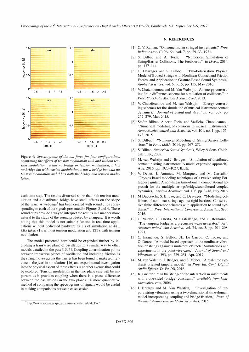
The effect due to the tension modulation can be seen more

clearly in Figure 4. The plots show spectrograms of the nut force

when the model is run with C2 string parameters and a greater

excitation amplitude of Ae = −0.8 N. It can be observed by com-

paring (a) and (b) to (c) and (d) that the tension modulation is no-

ticeable when the barrier is absent but has a larger effect when the

barrier is present. With these parameters the change in the shape of

the jvari is more significant than in the C3 case and is heard more

clearly in sound examples.

5. CONCLUSIONS

This paper shows how tension modulation, a distributed barrier

and the thread can be included in a model of the tanpura. The

model is proven to be unconditionally stable and to have a unique

solution to the non-linear vector equation that has to be solved at

1http://www.socasites.qub.ac.uk/mvanwalstijn/dafx17c/

DAFX-305

http://www.socasites.qub.ac.uk/mvanwalstijn/dafx17c/


Figure 4: Spectrograms of the nut force for four configurations

comparing the effects of tension modulation with and without ten-

sion modulation. a has no bridge or tension modulation, b has

no bridge but with tension modulation, c has a bridge but with no

tension modulation and d has both the bridge and tension modu-

lation.

each time step. The results discussed show that both tension mod-

ulation and a distributed bridge have small effects on the shape

of the jvari. A webpage2 has been created with sound clips corre-

sponding to each of the signals presented in Figures 3 and 4. These

sound clips provide a way to interpret the results in a manner more

natural to the study of the sound produced by a tanpura. It is worth

noting that this model is not suitable for use in real time appli-

cations without dedicated hardware as 1 s of simulation at 44.1kHz takes 81 s without tension modulation and 131 s with tension

modulation.

The model presented here could be expanded further by in-

cluding a transverse plane of oscillation in a similar way to other

models detailed in the past [13, 3]. Coupling at termination points

between transverse planes of oscillation and including friction as

the string moves across the barrier has been found to make a differ-

ence to the jvari in simulations [16] and experimental investigation

into the physical extent of these effects is another avenue that could

be explored. Tension modulation in the two plane case will be im-

portant as it provides coupling when there is a phase difference

between the oscillations in the two planes. A more quantitative

method of comparing the spectrograms of signals would be useful

in making comparisons between cases easier.

2http://www.socasites.qub.ac.uk/mvanwalstijn/dafx17c/

6. REFERENCES

[1] C. V. Raman, “On some Indian stringed instruments,” Proc.

Indian Assoc. Cultiv. Sci, vol. 7, pp. 29–33, 1921.

[2] S. Bilbao and A. Torin, “Numerical Simulation of

String/Barrier Collisions: The Fretboard.,” in DAFx, 2014,

pp. 137–144.

[3] C. Desvages and S. Bilbao, “Two-Polarisation Physical

Model of Bowed Strings with Nonlinear Contact and Friction

Forces, and Application to Gesture-Based Sound Synthesis,”

Applied Sciences, vol. 6, no. 5, pp. 135, May 2016.

[4] V. Chatziioannou and M. Van Walstijn, “An energy conserv-

ing finite difference scheme for simulation of collisions,” in

Proc. Stockholm Musical Acoust. Conf, 2013.

[5] V. Chatziioannou and M. van Walstijn, “Energy conserv-

ing schemes for the simulation of musical instrument contact

dynamics,” Journal of Sound and Vibration, vol. 339, pp.

262–279, Mar. 2015.

[6] Stefan Bilbao, Alberto Torin, and Vasileios Chatziioannou,

“Numerical modeling of collisions in musical instruments,”

Acta Acustica united with Acustica, vol. 101, no. 1, pp. 155–

173, 2015.

[7] S. Bilbao, “Numerical Modeling of String/Barrier Colli-

sions,” in Proc. ISMA, 2014, pp. 267–272.

[8] S. Bilbao, Numerical Sound Synthesis, Wiley & Sons, Chich-

ester, UK, 2009.

[9] M. van Walstijn and J. Bridges, “Simulation of distributed

contact in string instruments: A modal expansion approach,”

Aug. 2016, pp. 1023–1027, IEEE.

[10] V. Debut, J. Antunes, M. Marques, and M. Carvalho,

“Physics-based modeling techniques of a twelve-string Por-

tuguese guitar: A non-linear time-domain computational ap-

proach for the multiple-strings/bridge/soundboard coupled

dynamics,” Applied Acoustics, vol. 108, pp. 3–18, July 2016.

[11] M Ducceschi, S. Bilbao, and C. Desvages, “Modelling col-

lisions of nonlinear strings against rigid barriers: Conserva-

tive finite difference schemes with application to sound syn-

thesis,” in Proc. International Congress on Acoustics, Sept.

2016.

[12] C. Valette, C. Cuesta, M. Castellengo, and C. Besnainou,

“The tampura bridge as a precursive wave generator,” Acta

Acustica united with Acustica, vol. 74, no. 3, pp. 201–208,

1991.

[13] C. Issanchou, S. Bilbao, JL. Le Carrou, C. Touze, and

O. Doare, “A modal-based approach to the nonlinear vibra-

tion of strings against a unilateral obstacle: Simulations and

experiments in the pointwise case,” Journal of Sound and

Vibration, vol. 393, pp. 229–251, Apr. 2017.

[14] M. van Walstijn, J. Bridges, and S. Mehes, “A real-time syn-

thesis oriented tanpura model,” in Proc. Int. Conf. Digital

Audio Effects (DAFx-16), 2016.

[15] K. Guettler, “On the string-bridge interaction in instruments

with a one-sided (bridge) constraint,” available from knut-

sacoustics. com, 2006.

[16] J. Bridges and M. Van Walstijn, “Investigation of tan-

pura string vibrations using a two-dimensional time-domain

model incorporating coupling and bridge friction,” Proc. of

the third Vienna Talk on Music Acoustics, 2015.

DAFX-306

http://www.socasites.qub.ac.uk/mvanwalstijn/dafx17c/

Documents

Modal Based Tanpura Simulation: Combining Tension