Mobile Robot Vision Navigation & Localization Using Gist and Saliency

Chin-Kai Chang* Christian Siagian* Laurent Itti

Abstract— We present a vision-based navigation and localiza-tion system using two biologically-inspired scene understandingmodels which are studied from human visual capabilities: (1)Gist model which captures the holistic characteristics andlayoutof an image and (2) Saliency model which emulates the visualattention of primates to identify conspicuous regions in theimage. Here the localization system utilizes the gist featuresand salient regions to accurately localize the robot, whilethenavigation system uses the salient regions to perform visualfeedback control to direct its heading and go to a user-providedgoal location. We tested the system on our robot, Beobot2.0,in an indoor and outdoor environment with a route lengthof 36.67m (10,890 video frames) and 138.27m (28,971 frames),respectively. On average, the robot is able to drive within 3.68cmand 8.78cm (respectively) of the center of the lane.

I. INTRODUCTION

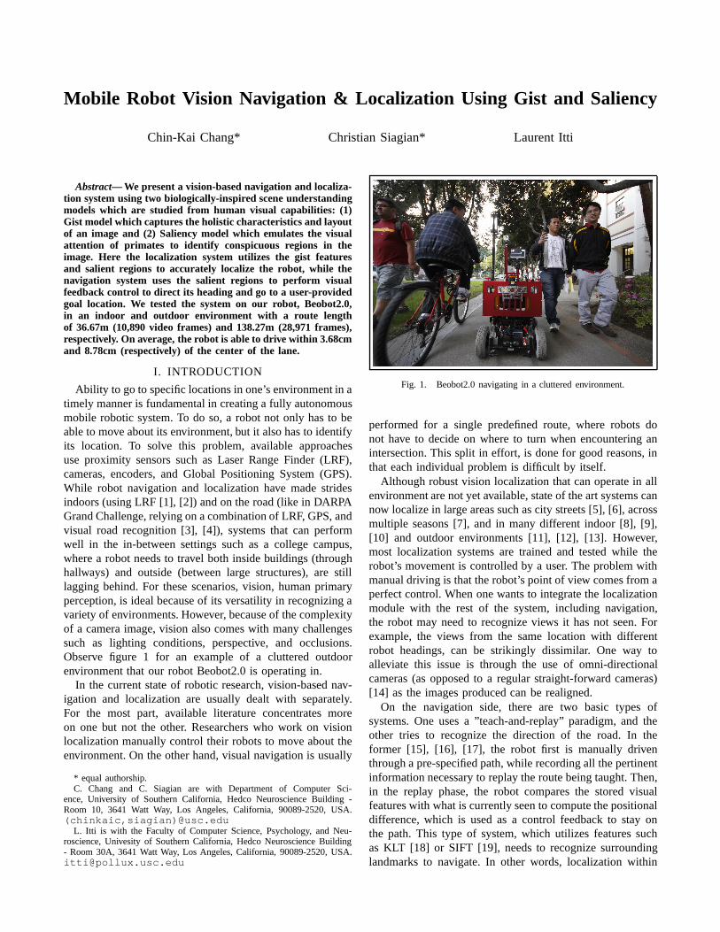
Ability to go to specific locations in one’s environment in atimely manner is fundamental in creating a fully autonomousmobile robotic system. To do so, a robot not only has to beable to move about its environment, but it also has to identifyits location. To solve this problem, available approachesuse proximity sensors such as Laser Range Finder (LRF),cameras, encoders, and Global Positioning System (GPS).While robot navigation and localization have made stridesindoors (using LRF [1], [2]) and on the road (like in DARPAGrand Challenge, relying on a combination of LRF, GPS, andvisual road recognition [3], [4]), systems that can performwell in the in-between settings such as a college campus,where a robot needs to travel both inside buildings (throughhallways) and outside (between large structures), are stilllagging behind. For these scenarios, vision, human primaryperception, is ideal because of its versatility in recognizing avariety of environments. However, because of the complexityof a camera image, vision also comes with many challengessuch as lighting conditions, perspective, and occlusions.Observe figure 1 for an example of a cluttered outdoorenvironment that our robot Beobot2.0 is operating in.

In the current state of robotic research, vision-based nav-igation and localization are usually dealt with separately.For the most part, available literature concentrates moreon one but not the other. Researchers who work on visionlocalization manually control their robots to move about theenvironment. On the other hand, visual navigation is usually

* equal authorship.C. Chang and C. Siagian are with Department of Computer Sci-

ence, University of Southern California, Hedco Neuroscience Building -Room 10, 3641 Watt Way, Los Angeles, California, 90089-2520, USA.(chinkaic,siagian)@usc.edu

L. Itti is with the Faculty of Computer Science, Psychology,and Neu-roscience, Univesity of Southern California, Hedco Neuroscience Building- Room 30A, 3641 Watt Way, Los Angeles, California, 90089-2520, USA.itti@pollux.usc.edu

Fig. 1. Beobot2.0 navigating in a cluttered environment.

performed for a single predefined route, where robots donot have to decide on where to turn when encountering anintersection. This split in effort, is done for good reasons, inthat each individual problem is difficult by itself.

Although robust vision localization that can operate in allenvironment are not yet available, state of the art systems cannow localize in large areas such as city streets [5], [6], acrossmultiple seasons [7], and in many different indoor [8], [9],[10] and outdoor environments [11], [12], [13]. However,most localization systems are trained and tested while therobot’s movement is controlled by a user. The problem withmanual driving is that the robot’s point of view comes from aperfect control. When one wants to integrate the localizationmodule with the rest of the system, including navigation,the robot may need to recognize views it has not seen. Forexample, the views from the same location with differentrobot headings, can be strikingly dissimilar. One way toalleviate this issue is through the use of omni-directionalcameras (as opposed to a regular straight-forward cameras)[14] as the images produced can be realigned.

On the navigation side, there are two basic types ofsystems. One uses a ”teach-and-replay” paradigm, and theother tries to recognize the direction of the road. In theformer [15], [16], [17], the robot first is manually driventhrough a pre-specified path, while recording all the pertinentinformation necessary to replay the route being taught. Then,in the replay phase, the robot compares the stored visualfeatures with what is currently seen to compute the positionaldifference, which is used as a control feedback to stay onthe path. This type of system, which utilizes features suchas KLT [18] or SIFT [19], needs to recognize surroundinglandmarks to navigate. In other words, localization within

the path (not throughout the environment) is required. Thisis done by retracing a sequence of keyframes, keeping trackof which frame the robot currently is at. When matchingbetween the current scene and keyframe fails, the systemhas to re-synchronize itself. This can take extra time asrematching from the start of the series is required.

On the other hand, road recognition systems, instead ofidentifying landmarks, try to recognize the road’s appearanceas well as boundaries. Some systems rely on recognizingroad edges (based on the intensity of images, for example)that separate the road from its surroundings [20]. Others doso by performing color and texture segmentation [21], [22].In addition, there are systems that combine both techniques[23], [24], [25] to extract the road region in the image.However, for these type of systems, the robot merely followsthe road and keeps itself within its boundaries, not knowingwhere it will ultimately end up.

If a system has both localization and navigation, we cancommand it to go to any goal location in the environmentby using the former to compute a route and the latter toexecute movements. In addition, such an integrated systemcan internally share resources (visual features, for one) tomake the overall system run more effectively. However, thisalso poses a challenging problem of integrating complex sub-systems. In spite of the difficulties, many vision localization[26] and navigation [15] systems have discussed that it isadvantageous to combine localization and navigation. Oursis such an implementation.

We present a mobile robot vision system that both lo-calizes and navigates by extending our previous work ofGist-Saliency localization [11]. Instead of just navigatingthrough a pre-specified path (like teach-and-replay), therobot can execute movements through any desired routesin the environment (e.g., routes generated by a planner).On the other hand, unlike teach-and-replay, a stand-alonelocalization system allows the navigation system to not beoverly sensitive to the temporal order of input images. Wetested the system (reported in section III) in both indoorand outdoor environments, each recorded multiple times tovalidate our approach.

II. DESIGN AND IMPLEMENTATIONS

Our presented mobile robot vision navigation and local-ization system (illustrated in figure 2) utilizes biologicallyinspired features: gist [27] and salient regions [11] of animage, obtained from a single straight-forward view camera(as opposed to omni-directional). Both features are computedin parallel, utilizing shared raw Visual Cortex visual featuresfrom the color, intensity and orientation domain [28], [29].Here we define gist as a holistic and concise feature vectorrepresentation of a scene, acquired over very short amountof time. Salient regions, on the other hand, are obtainedusing the saliency model [28], [29] which identifies partsof an image that readily capture the viewer’s attention. Asdemonstrated by previous testings [11], the likelihood thatthe same regions will pop out again when the robot revisitsparticular locations is quite high. The actual matching is done

through SIFT keypoints extracted within each salient region.It is important to note that matching keypoints within smallregion windows instead of a whole image makes the processmuch more efficient.

Our localization system [11], [30] estimates the robot’slocation in an environment represented by a topologicalmap. The map denotes paths as edges, and intersectionsas nodes. We also define the term segment as an orderedlist of edges with one edge connected to the next to forma continuous path (an example is the selected three-edgesegment, highlighted as a thicker green line, in the map infigure 2). Geographically speaking, a segment is usually aportion of a hallway, path, or road interrupted by a crossingor a physical barrier at both ends for a natural delineation.This grouping is motivated by the fact that views/layouts inone path segment are coarsely similar. Because of this, thesystem can use the gist vector to classify an input image toa segment.

After the system estimates the robot’s segment location,we then try to refine the coarse localization estimation bymatching the salient regions found in the input image withthe stored regions from our landmark database (obtainedduring training). Note that this process is much slower thansegment estimation but produces a higher localization reso-lution. At the end, both gist and salient region observationsare incorporated in a back-end probabilistic Monte CarloLocalization to produce the most likely current location.

In our training procedure, we run the robot through theenvironment once. There is no camera calibration nor manualselection of the landmarks. In addition, the training procedure[30] automatically clusters salient regions that portray thesame landmark. And, thus, a landmark, a real entity in theenvironment, is established by a set of salient regions. Ina sense, the regions become evidences that the landmarkexists. Furthermore, these regions are stored in the order ofdiscovery. That is, we keep a temporal order of the regions asseen when the robot traverses an environment. This becomesimportant when we try to navigate using these landmarks.

As a result of the compact topological map representation(figure 2), we do not localize the robot laterally on the lanenor do we have an accurate knowledge of the robot’s headingwith respect to the road. However, for each database salientregion, we do not only record its geographical location, butalso register its image coordinates to perform navigation.That is, we minimize the difference in image coordinatesbetween the input region and its corresponding databaseregion to bring and keep the robot at the “correct” position onthe lane (same position as during training). In the followingsub-section II-A, we describe the main contribution of thispaper, the navigation portion of the system and its interactionwith the localization component.

A. Navigation System

As shown in figure 2, localization and navigation run inparallel in the system. When a new set of input salient regionsarrive, the localization module starts its landmark databasesearch (denoted as1a in the figure). At the same time, the

98

6

5

3 4

1

2

Localization

Navigation

Motion Planner

Path

Planner

Identified

Landmark

Tracker

Input

Goal Location

Input

Landmark

Tracker

Lateral

Difference

Estimator

1a

1b

Fig. 2. Diagram of the overall vision navigation and localization system. From an input image the system extracts low-level features consisting ofcenter-surround color, intensity, and orientation that are computed in separate channels. They are then further processed to produce gist features and salientregions. We then compare them with previously obtained environment visual information to estimate the robots location. Furthermore the identified salientregions are used to direct the robot’s heading, to navigate itself to its destination.

navigation module also tracks these regions (1b). By trackingthem, when the regions are positively identified at a later time(usually database search finishes in the order of seconds),even if the robot has moved during the search process, we canstill locate the salient regions in the image. When a trackedregion is lost or moves away from the robot’s field of view,we simply tell the localizer to stop searching for a match.Note that, while the search is in progress, the gist-basedsegment estimation result, which is available instantaneouslyon every frame, is used to maintain the location belief.

When the database search concludes, if there is at least onematched region, the localization system informs the naviga-tion system that these regions can be used for navigation.The navigation system first transfers the regions tracked bythe input landmark tracker to the identified landmark tracker.A second tracker is needed to free up the first one fornewer, yet to be identified landmarks from the current frame.The identified landmark tracker keep track of the transferredregions so that we can utilize them for visual navigationcues for a period of time (until the newer landmarks arerecognized).

The navigation system calculates the image coordinate dif-ference (we call this lateral difference) between the trackedregion and the matched database region (section II-A.2) as afeedback to the motor controller. In addition, we also bias thesalient region matching (explained in section II-A.3) whenthe robot is at the intersections so that it can correctly direct

itself to the goal location.We start by explaining in details the salient region tracking

process in the following sub-section II-A.1.

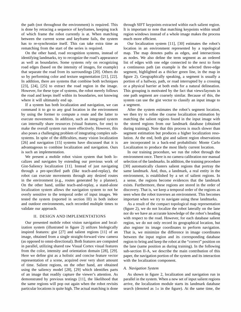
1) Salient Region Tracker:Figure 3 illustrates the salientregion tracking procedure. The tracker utilizes a templatematching algorithm (OpenCV implementation with squared-error distance) on conspicuity maps [28], [29] from the 7Visual Cortex sub-channels used in saliency and gist com-putation (see Figure 2; the sub-channels correspond to 4 edgeorientations, 2 color contrasts, and luminance contrast).Foreach region, we perform template matching on each map (7associated templates) before summing the resulting distancemap. The templates are initialized using 7x7 windows fromeach conspicuity map, centered around the salient point ofthe region. The conspicuity maps are 40x30 pixels in size,downsampled from the original 160x120 input image size,which is acceptable given that we are mostly tracking largesalient objects. We then weigh the summation based on thedistance from the previous time step for temporal filtering.The coordinate of the minimum value is the predicted newlocation.

In addition, in each frame, we update the templates forrobustness (lighting change, etc) using the following adaptiveequation:

Tt,i = .9 ∗ Tt−1,i + .1 ∗ Nt−1,i (1)

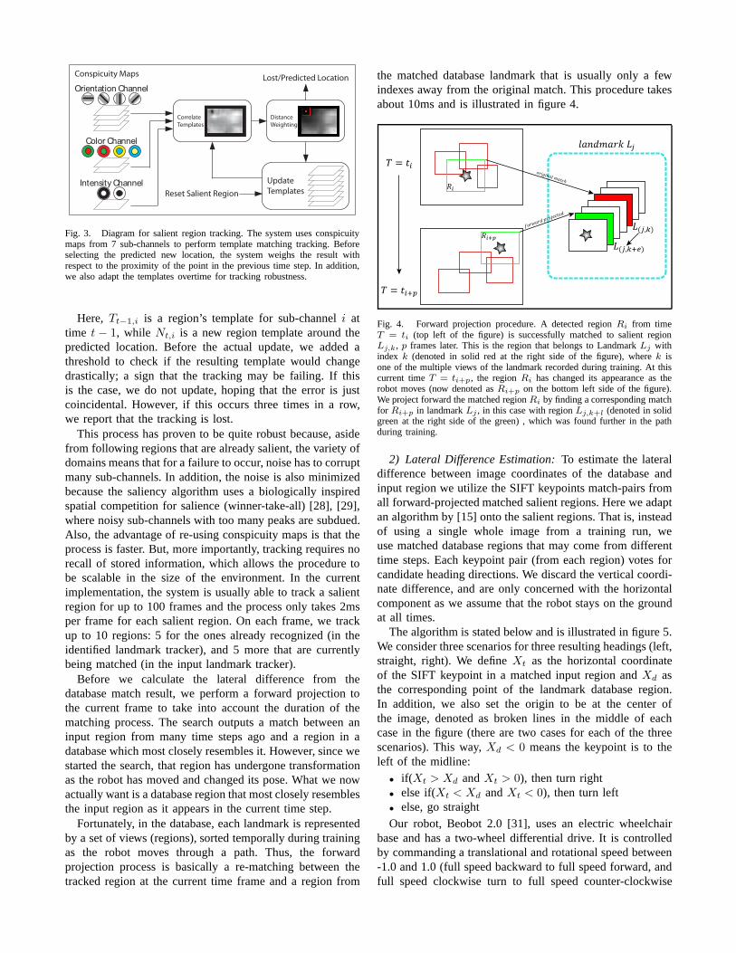
Fig. 3. Diagram for salient region tracking. The system usesconspicuitymaps from 7 sub-channels to perform template matching tracking. Beforeselecting the predicted new location, the system weighs theresult withrespect to the proximity of the point in the previous time step. In addition,we also adapt the templates overtime for tracking robustness.

Here, Tt−1,i is a region’s template for sub-channeli attime t − 1, while Nt,i is a new region template around thepredicted location. Before the actual update, we added athreshold to check if the resulting template would changedrastically; a sign that the tracking may be failing. If thisis the case, we do not update, hoping that the error is justcoincidental. However, if this occurs three times in a row,we report that the tracking is lost.

This process has proven to be quite robust because, asidefrom following regions that are already salient, the variety ofdomains means that for a failure to occur, noise has to corruptmany sub-channels. In addition, the noise is also minimizedbecause the saliency algorithm uses a biologically inspiredspatial competition for salience (winner-take-all) [28],[29],where noisy sub-channels with too many peaks are subdued.Also, the advantage of re-using conspicuity maps is that theprocess is faster. But, more importantly, tracking requires norecall of stored information, which allows the procedure tobe scalable in the size of the environment. In the currentimplementation, the system is usually able to track a salientregion for up to 100 frames and the process only takes 2msper frame for each salient region. On each frame, we trackup to 10 regions: 5 for the ones already recognized (in theidentified landmark tracker), and 5 more that are currentlybeing matched (in the input landmark tracker).

Before we calculate the lateral difference from thedatabase match result, we perform a forward projection tothe current frame to take into account the duration of thematching process. The search outputs a match between aninput region from many time steps ago and a region in adatabase which most closely resembles it. However, since westarted the search, that region has undergone transformationas the robot has moved and changed its pose. What we nowactually want is a database region that most closely resemblesthe input region as it appears in the current time step.

Fortunately, in the database, each landmark is representedby a set of views (regions), sorted temporally during trainingas the robot moves through a path. Thus, the forwardprojection process is basically a re-matching between thetracked region at the current time frame and a region from

the matched database landmark that is usually only a fewindexes away from the original match. This procedure takesabout 10ms and is illustrated in figure 4.

Fig. 4. Forward projection procedure. A detected regionRi from timeT = ti (top left of the figure) is successfully matched to salient regionLj,k, p frames later. This is the region that belongs to LandmarkLj withindex k (denoted in solid red at the right side of the figure), wherek isone of the multiple views of the landmark recorded during training. At thiscurrent timeT = ti+p, the regionRi has changed its appearance as therobot moves (now denoted asRi+p on the bottom left side of the figure).We project forward the matched regionRi by finding a corresponding matchfor Ri+p in landmarkLj , in this case with regionLj,k+l (denoted in solidgreen at the right side of the green) , which was found furtherin the pathduring training.

2) Lateral Difference Estimation:To estimate the lateraldifference between image coordinates of the database andinput region we utilize the SIFT keypoints match-pairs fromall forward-projected matched salient regions. Here we adaptan algorithm by [15] onto the salient regions. That is, insteadof using a single whole image from a training run, weuse matched database regions that may come from differenttime steps. Each keypoint pair (from each region) votes forcandidate heading directions. We discard the vertical coordi-nate difference, and are only concerned with the horizontalcomponent as we assume that the robot stays on the groundat all times.

The algorithm is stated below and is illustrated in figure 5.We consider three scenarios for three resulting headings (left,straight, right). We defineXt as the horizontal coordinateof the SIFT keypoint in a matched input region andXd asthe corresponding point of the landmark database region.In addition, we also set the origin to be at the center ofthe image, denoted as broken lines in the middle of eachcase in the figure (there are two cases for each of the threescenarios). This way,Xd < 0 means the keypoint is to theleft of the midline:

• if(Xt > Xd andXt > 0), then turn right• else if(Xt < Xd andXt < 0), then turn left• else, go straightOur robot, Beobot 2.0 [31], uses an electric wheelchair

base and has a two-wheel differential drive. It is controlledby commanding a translational and rotational speed between-1.0 and 1.0 (full speed backward to full speed forward, andfull speed clockwise turn to full speed counter-clockwise

Case1 Case1 Case1Case2 Case2 Case2

Le ft Stra igh t R ight

Fig. 5. Diagram for the voting scheme of navigation algorithm. Thereare three scenarios where the robot either moves left, straight, or right.For each scenario, there are two cases depending on the sign of Xd, thecorresponding point of the landmark database region. IfXd is to the leftof the center of the image (the dashed line that goes through the origin ofthe image coordinate system), thenXd < 0. The same applies forXt, thehorizontal coordinate of the keypoint in a matched input region. If Xt < Xd

andXt < 0, then turn left, else ifXt > Xd andXt > 0, then turn right.If neither, then go straight.

turn, respectively). We keep the translation at constant speed,while the turn speed is proportional to the average horizontalpixel difference. Note that the direction of turn is obtainedthrough the voting process above.

We find that our well-isolated salient regions make forclean correspondences that, for the most part, overwhelm-ingly agree with one of the three candidate directions.This is because, by using a compact region (as opposedto entire image like the original [15] algorithm), we avoidmatching other distracting portions of the image, which maybe occupied by dynamic obstacles, such as people.

3) Path Planning Biasing:What we have implemented sofar is to a policy that allows the robot to follow a continuousportion of the route, along the edges of the topological map.However, when the robot arrives at an intersection, theremay be multiple paths that stem out from it. The systemmay encounter a situation where it simultaneously recognizeregions that are going to lead the robot to two or moredifferent directions. For example, regions from the segmentthe robot is currently on may suggest it to continue to gostraight, while regions on an incident segment are going tosuggest it to make a turn. Here, we consider the task, theassigned goal location, by consulting with the path planner.

The system first checks with the localization sub-system tosee whether it is approaching an intersection. If so, the pathplanner then bias the localization system to first compareinput regions with database regions along the path to thegoal, before expanding the search. In addition, for subsequentmatches, we also prioritize comparison with database regionsthat are further along the intersection turn. This way, therobot is going to follow the same sequence of region matchesthat are established during training, which is critical forsuccessful turning.

At the end, for failure recovery, whenever the robot cannotrecognize any salient region for a period of time (we setfor five seconds), it stops and spins in place to scan itssurrounding. Note that the path planner re-plans every time

the localizer sends out a new current location to make correctadjustments even when the robot loses its way.

In summary, the procedure goes as follows: after the go-to-goal command is received from a user interface, the systemstarts by recognizing at least one salient region to localize.Once the robot is successful in doing so, it plans its pathto the goal location. The navigation system then uses theinitially recognized salient regions to properly move closer toits goal. During this movement, the robot continuously try toidentify newer regions to follow, to advance its mission. Thisprocedure repeats until the robot arrives at its destination.

A snapshot of how the overall system generates robotmotion from a frame can be observed in figure 6.

III. TESTING AND RESULTS

We test the system using our robot, Beobot 2.0 [31](observe figure 1), which is 57cm in length and 60cm inwidth. The camera itself is about 117cm above the ground.Beobot 2.0 has a computing cluster of eight 2.2GHz Core2Duo processors. We use four computers for localization, onefor navigation, three for future use.

We select two different sites, an indoor and an out-door environment, for testing. The first is the hallwaysof 27.13x27.13m HNB building, with a corridor width of1.83m. The path forms a square with 90 degree angleswhen turning from one segment to another (observe the mapin figure 6). The second one is the 69.49x18.29m outdoorengineering quad (Equad), where there are buildings as wellas trees, with a pathway width of 3m. Snapshots of eachenvironment are shown in figure 7.

Despite the fact that, in our testing environments, weonly map one option on each junction, the path planner stillperform its job of selecting that option. Note that picking theright junction to proceed to the goal trivial using shortest-path in the graph-based topological map. On the other hand,the actual turning execution on the chosen junction is muchmore difficult.

Fig. 7. Scene examples of the HNB and Equad environment.

For each environment, we run the robot through all pathsonce for training. We then run the robot five times indoorsand three times outdoors for the testing phase. During testing,we record the trajectory of the robot odometry and itslocalization belief. We set the ground truth of the robotlocation by using manually calibrated odometry reading. Thebaseline for an ideal navigation itself is the center of the path.

The results for both sites are shown in table I, whichspecifies the sites’ dimensions and length of traversal. In

S2 S3 S4

SEG1

SEG3

SEG4SEG2

S1

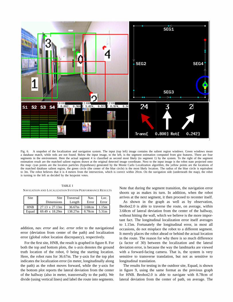
Fig. 6. A snapshot of the localization and navigation system. The input (top left) image contains the salient region windows. Green windows meana database match, while reds are not found. Below the input image, to the left, is the segment estimation computed from gist features. There are foursegments in the environment. Here the actual segment 4 is classified as second most likely (to segment 1) by the system. To the right of the segmentestimation result are the matched salient regions drawn at the original detected image coordinate. Next to the input image is the robot state projected ontothe map: cyan points are the location particles (hypotheses) generated by the Monte Carlo Localization algorithm, the yellow points are the locations ofthe matched database salient region, the green circle (the center of the blue circle) is the most likely location. The radius of the blue circle is equivalentto 3m. The robot believes that it is 4 meters from the intersection, which is correct within 20cm. On the navigation side (underneath the map), the robotis turning to the left as decided by the keypoint votes.

TABLE I

NAVIGATION AND LOCALIZATION SYSTEM PERFORMANCERESULTS

Site Site Traversal Nav. Loc.Dimensions Length Error Error

HNB 27.13 x 27.13m 36.67m 3.68cm 1.15mEquad 69.49 x 18.29m 138.27m 8.78cm 5.31m

addition,nav. error and loc. error refer to the navigationalerror (deviation from center of the path) and localizationerror (global robot location discrepancy), respectively.

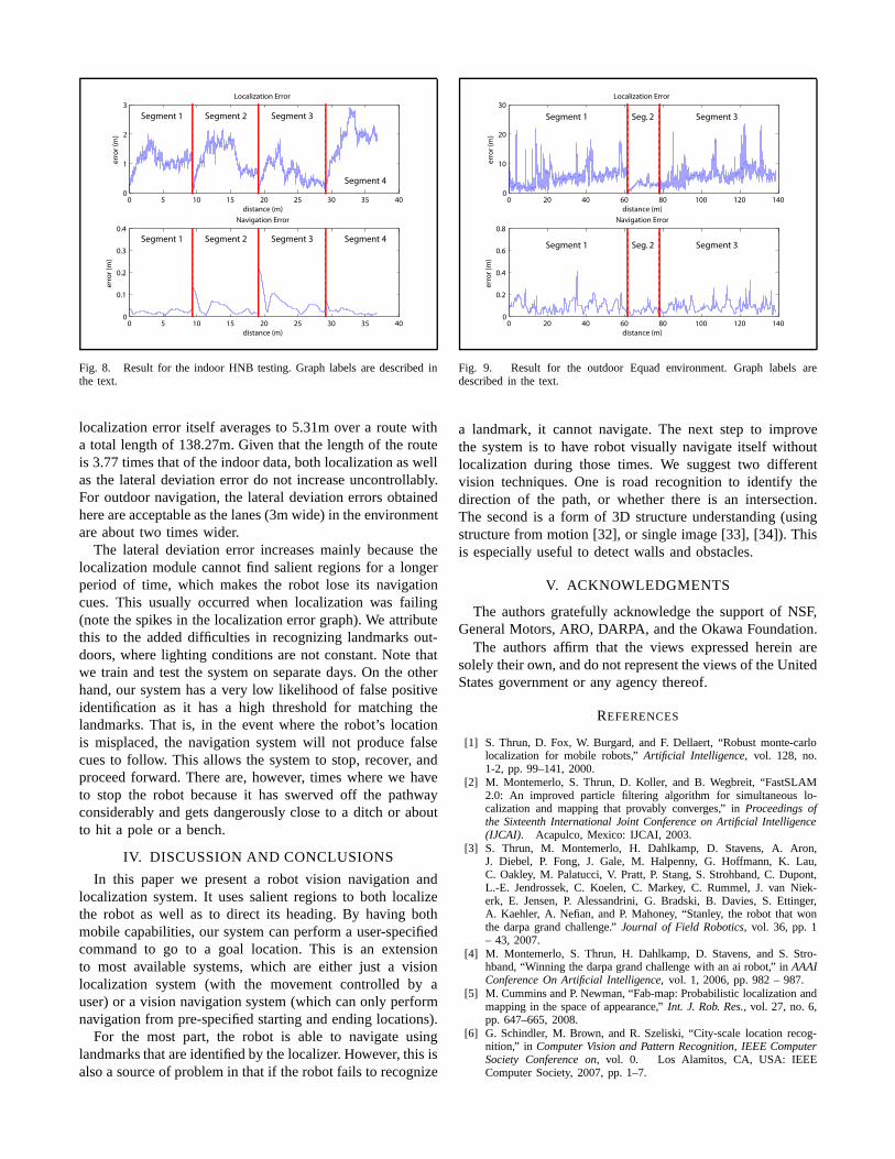
For the first site, HNB, the result is graphed in figure 8. Forboth the top and bottom plots, the x-axis denotes the groundtruth location of the robot, 0 being the starting location.Here, the robot runs for 36.67m. The y-axis for the top plotindicates the localization error (in meter, longitudinally alongthe path) as the robot moves forward, while the y-axis forthe bottom plot reports the lateral deviation from the centerof the hallway (also in meter, transversally to the path). Wedivide (using vertical lines) and label the route into segments.

Note that during the segment transition, the navigation errorshoots up as makes its turn. In addition, when the robotarrives at the next segment, it then proceed to recenter itself.

As shown in the graph as well as by observation,Beobot2.0 is able to traverse the route, on average, within3.68cm of lateral deviation from the center of the hallway,without hitting the wall, which we believe is the more impor-tant fact. The longitudinal localization error itself averagesto 1.15m. Fortunately the longitudinal error, in most alloccasions, do not misplace the robot to a different segment.It merely places the robot ahead or behind the actual locationin the route. The reason for why there is so much difference(a factor of 30) between the localization and the lateraldeviation error, is because the way the landmarks are viewedwith a forward-facing camera. That is, the system is verysensitive to transverse translation, but not as sensitive tolongitudinal translation.

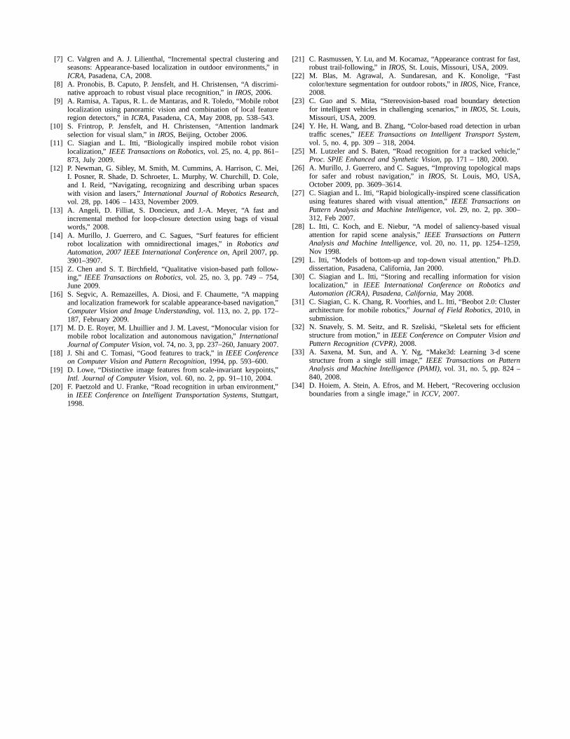
The results for testing in the outdoor site, Equad, is shownin figure 9, using the same format as the previous graphfor HNB. Beobot2.0 is able to navigate with 8.78cm oflateral deviation from the center of path, on average. The

0 5 10 15 20 25 30 35 400

1

2

3

Localization Error

distance (m)

err

or

(m)

0 5 10 15 20 25 30 35 400

0.1

0.2

0.3

0.4

Navigation Error

distance (m)

err

or

(m)

Segment 1

Segment 4

Segment 2 Segment 3

Segment 1 Segment 4Segment 2 Segment 3

Fig. 8. Result for the indoor HNB testing. Graph labels are described inthe text.

localization error itself averages to 5.31m over a route witha total length of 138.27m. Given that the length of the routeis 3.77 times that of the indoor data, both localization as wellas the lateral deviation error do not increase uncontrollably.For outdoor navigation, the lateral deviation errors obtainedhere are acceptable as the lanes (3m wide) in the environmentare about two times wider.

The lateral deviation error increases mainly because thelocalization module cannot find salient regions for a longerperiod of time, which makes the robot lose its navigationcues. This usually occurred when localization was failing(note the spikes in the localization error graph). We attributethis to the added difficulties in recognizing landmarks out-doors, where lighting conditions are not constant. Note thatwe train and test the system on separate days. On the otherhand, our system has a very low likelihood of false positiveidentification as it has a high threshold for matching thelandmarks. That is, in the event where the robot’s locationis misplaced, the navigation system will not produce falsecues to follow. This allows the system to stop, recover, andproceed forward. There are, however, times where we haveto stop the robot because it has swerved off the pathwayconsiderably and gets dangerously close to a ditch or aboutto hit a pole or a bench.

IV. DISCUSSION AND CONCLUSIONS

In this paper we present a robot vision navigation andlocalization system. It uses salient regions to both localizethe robot as well as to direct its heading. By having bothmobile capabilities, our system can perform a user-specifiedcommand to go to a goal location. This is an extensionto most available systems, which are either just a visionlocalization system (with the movement controlled by auser) or a vision navigation system (which can only performnavigation from pre-specified starting and ending locations).

For the most part, the robot is able to navigate usinglandmarks that are identified by the localizer. However, this isalso a source of problem in that if the robot fails to recognize

0 20 40 60 80 100 120 1400

10

20

30

Localization Error

distance (m)

err

or

(m)

0 20 40 60 80 100 120 1400

0.2

0.4

0.6

0.8

Navigation Error

distance (m)

err

or

(m)

Seg. 2 Segment 3Segment 1

Seg. 2 Segment 3Segment 1

Fig. 9. Result for the outdoor Equad environment. Graph labels aredescribed in the text.

a landmark, it cannot navigate. The next step to improvethe system is to have robot visually navigate itself withoutlocalization during those times. We suggest two differentvision techniques. One is road recognition to identify thedirection of the path, or whether there is an intersection.The second is a form of 3D structure understanding (usingstructure from motion [32], or single image [33], [34]). Thisis especially useful to detect walls and obstacles.

V. ACKNOWLEDGMENTS

The authors gratefully acknowledge the support of NSF,General Motors, ARO, DARPA, and the Okawa Foundation.

The authors affirm that the views expressed herein aresolely their own, and do not represent the views of the UnitedStates government or any agency thereof.

REFERENCES

[1] S. Thrun, D. Fox, W. Burgard, and F. Dellaert, “Robust monte-carlolocalization for mobile robots,”Artificial Intelligence, vol. 128, no.1-2, pp. 99–141, 2000.

[2] M. Montemerlo, S. Thrun, D. Koller, and B. Wegbreit, “FastSLAM2.0: An improved particle filtering algorithm for simultaneous lo-calization and mapping that provably converges,” inProceedings ofthe Sixteenth International Joint Conference on ArtificialIntelligence(IJCAI). Acapulco, Mexico: IJCAI, 2003.

[3] S. Thrun, M. Montemerlo, H. Dahlkamp, D. Stavens, A. Aron,J. Diebel, P. Fong, J. Gale, M. Halpenny, G. Hoffmann, K. Lau,C. Oakley, M. Palatucci, V. Pratt, P. Stang, S. Strohband, C.Dupont,L.-E. Jendrossek, C. Koelen, C. Markey, C. Rummel, J. van Niek-erk, E. Jensen, P. Alessandrini, G. Bradski, B. Davies, S. Ettinger,A. Kaehler, A. Nefian, and P. Mahoney, “Stanley, the robot that wonthe darpa grand challenge.”Journal of Field Robotics, vol. 36, pp. 1– 43, 2007.

[4] M. Montemerlo, S. Thrun, H. Dahlkamp, D. Stavens, and S. Stro-hband, “Winning the darpa grand challenge with an ai robot,”in AAAIConference On Artificial Intelligence, vol. 1, 2006, pp. 982 – 987.

[5] M. Cummins and P. Newman, “Fab-map: Probabilistic localization andmapping in the space of appearance,”Int. J. Rob. Res., vol. 27, no. 6,pp. 647–665, 2008.

[6] G. Schindler, M. Brown, and R. Szeliski, “City-scale location recog-nition,” in Computer Vision and Pattern Recognition, IEEE ComputerSociety Conference on, vol. 0. Los Alamitos, CA, USA: IEEEComputer Society, 2007, pp. 1–7.

[7] C. Valgren and A. J. Lilienthal, “Incremental spectral clustering andseasons: Appearance-based localization in outdoor environments,” inICRA, Pasadena, CA, 2008.

[8] A. Pronobis, B. Caputo, P. Jensfelt, and H. Christensen,“A discrimi-native approach to robust visual place recognition,” inIROS, 2006.

[9] A. Ramisa, A. Tapus, R. L. de Mantaras, and R. Toledo, “Mobile robotlocalization using panoramic vision and combination of local featureregion detectors,” inICRA, Pasadena, CA, May 2008, pp. 538–543.

[10] S. Frintrop, P. Jensfelt, and H. Christensen, “Attention landmarkselection for visual slam,” inIROS, Beijing, October 2006.

[11] C. Siagian and L. Itti, “Biologically inspired mobile robot visionlocalization,” IEEE Transactions on Robotics, vol. 25, no. 4, pp. 861–873, July 2009.

[12] P. Newman, G. Sibley, M. Smith, M. Cummins, A. Harrison,C. Mei,I. Posner, R. Shade, D. Schroeter, L. Murphy, W. Churchill, D. Cole,and I. Reid, “Navigating, recognizing and describing urbanspaceswith vision and lasers,”International Journal of Robotics Research,vol. 28, pp. 1406 – 1433, November 2009.

[13] A. Angeli, D. Filliat, S. Doncieux, and J.-A. Meyer, “A fast andincremental method for loop-closure detection using bags of visualwords,” 2008.

[14] A. Murillo, J. Guerrero, and C. Sagues, “Surf features for efficientrobot localization with omnidirectional images,” inRobotics andAutomation, 2007 IEEE International Conference on, April 2007, pp.3901–3907.

[15] Z. Chen and S. T. Birchfield, “Qualitative vision-basedpath follow-ing,” IEEE Transactions on Robotics, vol. 25, no. 3, pp. 749 – 754,June 2009.

[16] S. Segvic, A. Remazeilles, A. Diosi, and F. Chaumette, “A mappingand localization framework for scalable appearance-basednavigation,”Computer Vision and Image Understanding, vol. 113, no. 2, pp. 172–187, February 2009.

[17] M. D. E. Royer, M. Lhuillier and J. M. Lavest, “Monocularvision formobile robot localization and autonomous navigation,”InternationalJournal of Computer Vision, vol. 74, no. 3, pp. 237–260, January 2007.

[18] J. Shi and C. Tomasi, “Good features to track,” inIEEE Conferenceon Computer Vision and Pattern Recognition, 1994, pp. 593–600.

[19] D. Lowe, “Distinctive image features from scale-invariant keypoints,”Intl. Journal of Computer Vision, vol. 60, no. 2, pp. 91–110, 2004.

[20] F. Paetzold and U. Franke, “Road recognition in urban environment,”in IEEE Conference on Intelligent Transportation Systems, Stuttgart,1998.

[21] C. Rasmussen, Y. Lu, and M. Kocamaz, “Appearance contrast for fast,robust trail-following,” in IROS, St. Louis, Missouri, USA, 2009.

[22] M. Blas, M. Agrawal, A. Sundaresan, and K. Konolige, “Fastcolor/texture segmentation for outdoor robots,” inIROS, Nice, France,2008.

[23] C. Guo and S. Mita, “Stereovision-based road boundary detectionfor intelligent vehicles in challenging scenarios,” inIROS, St. Louis,Missouri, USA, 2009.

[24] Y. He, H. Wang, and B. Zhang, “Color-based road detection in urbantraffic scenes,”IEEE Transactions on Intelligent Transport System,vol. 5, no. 4, pp. 309 – 318, 2004.

[25] M. Lutzeler and S. Baten, “Road recognition for a tracked vehicle,”Proc. SPIE Enhanced and Synthetic Vision, pp. 171 – 180, 2000.

[26] A. Murillo, J. Guerrero, and C. Sagues, “Improving topological mapsfor safer and robust navigation,” inIROS, St. Louis, MO, USA,October 2009, pp. 3609–3614.

[27] C. Siagian and L. Itti, “Rapid biologically-inspired scene classificationusing features shared with visual attention,”IEEE Transactions onPattern Analysis and Machine Intelligence, vol. 29, no. 2, pp. 300–312, Feb 2007.

[28] L. Itti, C. Koch, and E. Niebur, “A model of saliency-based visualattention for rapid scene analysis,”IEEE Transactions on PatternAnalysis and Machine Intelligence, vol. 20, no. 11, pp. 1254–1259,Nov 1998.

[29] L. Itti, “Models of bottom-up and top-down visual attention,” Ph.D.dissertation, Pasadena, California, Jan 2000.

[30] C. Siagian and L. Itti, “Storing and recalling information for visionlocalization,” in IEEE International Conference on Robotics andAutomation (ICRA), Pasadena, California, May 2008.

[31] C. Siagian, C. K. Chang, R. Voorhies, and L. Itti, “Beobot 2.0: Clusterarchitecture for mobile robotics,”Journal of Field Robotics, 2010, insubmission.

[32] N. Snavely, S. M. Seitz, and R. Szeliski, “Skeletal setsfor efficientstructure from motion,” inIEEE Conference on Computer Vision andPattern Recognition (CVPR), 2008.

[33] A. Saxena, M. Sun, and A. Y. Ng, “Make3d: Learning 3-d scenestructure from a single still image,”IEEE Transactions on PatternAnalysis and Machine Intelligence (PAMI), vol. 31, no. 5, pp. 824 –840, 2008.

[34] D. Hoiem, A. Stein, A. Efros, and M. Hebert, “Recoveringocclusionboundaries from a single image,” inICCV, 2007.