170C Market Place Boulevard • Knoxville, TN 37922 • Tel: 865-691-5540 • Fax: 865-691-5046 www.enernex.com

Final Report - 2006 Minnesota Wind Integration Study

Volume I

Prepared for:

The Minnesota Public Utilities Commission

c/o Mr. Ken Wolf Reliability Administrator

121 7th Place E. Suite 350

Saint Paul, MN 55101-2147

Prepared by:

EnerNex Corporation 170C Market Place Boulevard

Knoxville, Tennessee 37922 Tel: (865) 691-5540

FAX: (865) 691-5046 www.enernex.com

In Collaboration with:

The Midwest Independent System Operator

November 30, 2006

Page i

PROJECT TEAM

EnerNex Corporation

Robert Zavadil – Project Manager

Jack King

Nader Samaan

Jeff Lamoree

WindLogics

Mark Ahlstrom

Dr. Bruce Lee

Dr. Dennis Moon

Dr. Cathy Finley

Dave Savage

Ryan Koehnen

Patrick Heinis

Midwest Independent System Operator

Dale Osborn

Chuck Tyson

Zheng Zhou

Minnesota Public Utilities Commission

Ken Wolf – Reliability Administrator

Matt Schuerger – Technical Advisor

Page ii

Technical Review Committee

Steve Beuning, Xcel Energy

Ed DeMeo, Utility Wind Integration Group

John Dunlop, American Wind Energy Association

Dave Geschwind, Southern Minnesota Municipal Power Agency

Brian Glover, Mid-Continent Area Power Pool/ Midwest Reliability Organization

Jeff Haase, MN Department of Commerce

Daryl Hanson, Otter Tail Power

Mike Jacobs, American Wind Energy Association

Paul Johnson, Minnesota Power

Brendan Kirby, Oak Ridge National Laboratory

Andrew Lucero, Minnesota Power

David Lemmons, Xcel Energy

Michael McMullen, Xcel Energy

Mike Michaud, Community-Based Energy Development

Michael Milligan, National Renewable Energy Laboratory

Dale Osborn, Midwest Independent System Operator

Brian Parsons, National Renewable Energy Laboratory

Rick Peterson, Xcel Energy

Dean Schiro, Xcel Energy

Matt Schuerger (TRC Chair), Technical Advisor to the MN PUC

John Seidel, Mid-Continent Area Power Pool / Midwest Reliability Organization

Stan Selander, Great River Energy

Charlie Smith, Utility Wind Integration Group

JoAnn Thompson, Otter Tail Power

Jerry Tielke, Missouri River Energy Services

Lise Trudeau, Minnesota Department of Commerce

Chuck Tyson, Midwest Independent System Operator

Ray Wahle, Missouri River Energy Services

Ken Wolf, Minnesota Public Utilities Commission

Zheng Zhou, Midwest Independent System Operator

Page iii

Contents – Volume I

Project Team i Preface x Executive Summary xiii Approach xiv Models and Assumptions xvi Reliability Impacts xvii Operating Impacts xviii Study Conclusions xxi Project and Report Overview xxii Section 1 Introduction 1 Characteristics of Wind Generation 1 Overview of Utility System Operations 2

Short-Term Planning and Real-Time Operation 2 Wind Generation and Long-Term Power System Reliability 4 Influence of the MISO Market on Minnesota Utility Company Operations 5

Project Organization 5 Report Overview 6 Section 2 Characterizing the Minnesota Wind Resource 7 Synthesis of Wind Speed Data for the MN Wind Generation Scenarios 7 Wind Generation Forecasts 13 Spatial and Geographic Diversity 13 Section 3 Models and Assumptions 16 MISO Market Structure 16 Analytical Approach 18

Reliability Analysis 18 Operating Impacts 21

Study Data and Assumptions 23 Modeling Minnesota Electric Load in 2020 25 Developing Wind Generation Data 27

Estimating Reserve and Other Operational Requirements 32 Regulating Reserves 33 Contingency Reserves 35 Load Following 36 Operating Reserve “Margin" 38

Page iv

Discussion 40 Modeling Time-Varying Reserve Requirements in PROMOD 41 Section 4 Reliability Impacts 46 GE-MARS Analysis 48

Results 48 Discussion 51

Results from Marelli 53 Discussion 57 Summary 60 Section 5 Operating Impacts 61 Overview 61 “Base” Cases 61 Reserve Costs 66 Market Impacts 68 The Cost of Integrating Wind Generation 71

Background 71 Results of PROMOD Cases 72

Impacts of Wind Generation on Unit Utilization and Transactions 72 Effect of Wind Generation Forecasting 73 Section 6 Conclusions 76 Section 7 References 78 Appendix A – West RSG Study Assumptions 80 Introduction 80 Fuel Forecast 80 Load Forecast 81 Generating Units and parameters 81

Existing Units 81 New units for West RSG study 81

Transmission Upgrades 82 Appendix B - West RSG Study New Generating Units 84 Appendix C – Method for Converting Wind Speed Data to Wind Generation 86

Page v

Figures

Figure 1: Location of “proxy towers” (model data extraction points) on inner grid. xv Figure 2: Unit commitment costs for three penetration levels and pattern years. Cost of

incremental operating reserves is embedded. xx Figure 3: Inner and outer nested grids used in MM5 meteorological simulation model. 9 Figure 4: Location of “proxy towers” (model data extraction points) on inner grid (yellow are

existing / contracted). 10 Figure 5: Location of “proxy towers” in MM5 nested grid model. Legend: - Red: Existing wind

generation; Green: Additional sites for 15% scenario; Yellow: Additional sites for 20% scenario; Blue: Additional sites for 25% scenario 11

Figure 6: Mean annual wind speed at 80 m AGL (r) and net annual capacity factor (l). 12 Figure 7: Mean annual wind speed at 80 m AGL (r) and net annual capacity factor assuming

14% losses from gross and Vestas V82 1.65 MW MkII power curve, (left) by county.12 Figure 8: Correlation of wind generation power changes to distance between plants/turbines.

From NREL/CP-500-26722, July, 1999 14 Figure 9: Reduction in hourly variability (change) of wind generation as wind generation over

the region is aggregated. 14 Figure 10: Annual histogram of occurrence percentage of hourly capacity factor for four levels of

geographic dispersion. Data is based on hourly performance for the Vestas V82 1.65 MW turbine and reflects gross capacity factors. See legend for specific geographic dispersion scenario. Note: MN_SW = Minnesota Southwest, MN_SE = Minnesota Southeast, MN_NE = Minnesota Northeast, and ND_C = North Dakota Central. 15

Figure 11: Structure of MISO market and reliability footprints. (from MISO Business Practices Manual) Note: Southern Minnesota Municipal Power Agency is now a MISO market participant; LGE is leaving MISO). 18

Figure 12: MISO structure for generation dispatch and control. 19 Figure 13: Determining wind generation capacity value by LOLP analysis. 21 Figure 14: Flowchart for Technical Analysis 23 Figure 15: Overview of West RSG study PROMOD model, used as the basis for this study.

Companies shown in red are represented in detail. 24 Figure 16: Single turbine versus “plant” power curves, from empirical data for 30 MW plant 28 Figure 17: Wind generation regions and network injection buses 29 Figure 18: Installed wind generation capacity by region and scenario 31 Figure 19: Wind energy production by region and scenario. 31

Page vi

Figure 20: Approximate regulating requirements for a Balancing Authority as a function of peak demand. 33

Figure 21: Variation of the standard deviation of the regulation characteristic for each of nine sample days by number of turbines comprising measurement group. 34

Figure 22: Five-minute variability – 15% wind generation 37 Figure 23: Five-minute variability – 20% wind generation 37 Figure 24: Five-minute variability – 25% wind generation 38 Figure 25: Next-hour deviation from persistence forecast – 15% wind generation 39 Figure 26: Next-hour deviation from persistence forecast – 20% wind generation 39 Figure 27: Next-hour deviation from persistence forecast – 25% wind generation 40 Figure 28: Hourly wind generation changes as functions of production level. 15% (left);

20% (middle); 25% (right) 42 Figure 29: Empirical next-hour wind variability curves (top) and quadratic approximation (middle)

and equations (bottom). Vertical axis quantity on charts is standard deviation. 43 Figure 30: Illustration of time varying “operating reserve margin” developed from statistical

analysis of hourly wind generation variations. 44 Figure 31: New conventional generation in West RSG expansion plan 47 Figure 32: Wind generation capacity factor for varying number of highest load hours. (2003,

2004, and 2005 wind and load patterns) 49 Figure 33: LOLE for Minnesota Area based on 2003 load and wind patterns 50 Figure 34: LOLE for Minnesota Area based on 2004 load and wind patterns 50 Figure 35: LOLE for Minnesota Area based on 2005 load and wind patterns 50 Figure 36: Hourly wind production for highest 100 load hours of year (20% scenario) 52 Figure 37: LOLH (Loss of Load Hours) from Marelli analysis for 2003 wind and load patterns 53 Figure 38: LOLH (Loss of Load Hours) from Marelli analysis for 2004 wind and load patterns 54 Figure 39: LOLH (Loss of Load Hours) from Marelli analysis for 2005 wind and load patterns 54 Figure 40: GE-MARS results for isolated MN system; 2003 wind and load patterns 55 Figure 41 GE-MARS results for isolated MN system; 2004 wind and load patterns 55 Figure 42: GE-MARS results for isolated MN system; 2005 wind and load patterns 55 Figure 43: Weekly LOLP results for 2003 for GE-MARS and Marelli 57 Figure 44: Weekly LOLP results for 2004 for GE-MARS and Marelli 58 Figure 45: Weekly LOLP results for 2005 for GE-MARS and Marelli 59 Figure 46: Production cost for Minnesota companies as a function of wind penetration and

operating reserve level. 63 Figure 47: Load payments for Minnesota companies as a function of wind penetration and

operating reserve level. 64 Figure 48: Gas unit capacity factor as functions of wind generation and operating reserve level 65

Page vii

Figure 49: Coal unit capacity factor as functions of wind generation and operating reserve level66 Figure 50: Production cost as a function of wind penetration and operating reserve level. 67 Figure 51: Wind generation impact on relative locational marginal price – Great River Energy and

Minnkota hubs 69 Figure 52: Wind generation impact on relative locational marginal price – Minnesota Power and

Xcel Energy hubs 70 Figure 53: Wind generation impact on relative locational marginal price – Ottertail Power and

Southern Minnesota Municipal Power Agency hubs 70 Figure 54: Unit commitment costs for three penetration levels and pattern years. Cost of

incremental operating reserves is embedded. 72 Figure 55: Effect of wind generation forecast on Minnesota company production and load costs74 Figure 56: Turbine power curve used for calculating generation data from wind speed

measurements. 86 Figure 57: Empirical “Power Curve” for wind plant from measured values. 87 Figure 58: Wind plant “power curve” calculated from 10-minute wind speed values. 87 Figure 59: Calculated vs. Measured wind generation. 88 Figure 60: Measured and calculated plant power curves. 89 Figure 61: Exponential modification of measured wind speed. 89 Figure 62: Measured and modified calculated plant power curves. 90 Figure 63: Comparison of measured wind generation to that calculated with wind speed

modification. 91

Page viii

Tables

Table 1: Estimated Operating Reserve Requirement for MN Balancing Authority – 2020 Load xvii Table 2: Capacity Value of Wind Generation for 2003 Load and Wind Patterns xviii Table 3: Capacity Value of Wind Generation for 2004 Load and Wind Patterns xviii Table 4: Capacity Value of Wind Generation for 2005 Load and Wind Patterns xviii Table 5: Incremental Reserve Cost for 20% Wind Case, 2004 Patterns xx Table 6: 2020 Projections of Minnesota electric retail sales and wind generation at assumed

annual capacity factors. 8 Table 7: Control Areas within MISO’s Reliability Authority Footprint 20 Table 8: Minnesota retail sales by company for CY2004 and Total Retail Sales assumptions for

study 25 Table 9: Loads by Company from PROMOD West RSG case for 2020. 26 Table 10: Meteorological Tower Assignments by Region and Scenario 30 Table 11: Installed Capacity by Region and Penetration Scenario 31 Table 12: Adjustment of Wind Generation Model to Achieve Study Target Penetrations 32 Table 13: Characteristics of Wind Generation Model – Capacity Factor by Season & Region 32 Table 14: Estimated Regulating Requirements for Individual MN Balancing Authorities and

Aggregate 34 Table 15: Estimated Regulation Requirement for MN Balancing Authority in 2020 35 Table 16: Summary of Five-minute Variability 36 Table 17: Next-hour Deviation from Persistence Forecast by Wind Generation Scenario 38 Table 18: Estimated Operating Reserve Requirement for MN Balancing Authority – 2020 Load 41 Table 19: Standard Deviation of One-Hour Production Changes by Generation Level 42 Table 20: Characteristics of Additional Variable Reserve 45 Table 21: ELCC Results for 2003 Wind and Load Patterns 51 Table 22: ELCC Results for 2004 Wind and Load Patterns 51 Table 23: ELCC Results for 2005 Wind and Load Patterns 51 Table 24: Comparison of ELCC Results from GE-MARS and Marelli LOLP Analysis 56 Table 25: Capacity Accreditation of Wind Generation for Study per MAPP RSG Methodology 60 Table 26: Incremental Reserve Cost for 20% Wind Case, 2004 Patterns 68 Table 27: Wind Generation Impacts on Energy Market Metrics – 2004 Wind and Load Patterns 69

Page ix

Table 28: MN Company Emissions for ”No Wind” case and offsets for wind generation levels 70 Table 29: Load and Production for 20% Case, 2004 Patterns 73 Table 30: Summary of Case Results for various treatment of wind in unit commitment (2004

wind and load patterns) 74 Table 31: Summary of Unit Commitment Cases: Variable Reserve, Load and Wind Forecast

Error in Unit Commitment 75 Table 32 81 Table 33: New Transmission Lines in West RSG Study 83

Page x

PREFACE

In May of 2005 the Minnesota Legislature adopted a requirement for a Wind Integration Study of the impacts on reliability and costs associated with increasing wind capacity to 20% of Minnesota retail electric energy sales by the year 2020, and to identify and develop options for utilities to use to manage the intermittent nature of wind resources1. The law authorizes and directs the Reliability Administrator to manage the study. In July of 2005 the Minnesota Public Utilities Commission ordered2: 1) All Minnesota electric utilities to participate in the study; 2) The Minnesota electric utilities to contract jointly with an independent firm to conduct the study and to cooperate with completion of the study; and 3) The Minnesota electric utilities to use the study results to estimate impacts on their electric rates of increasing wind capacity to 20 percent and incorporate the study’s findings in resource plans and renewable energy objectives reports.

In the summer of 2005, a thorough and complete review of the current status and understanding of integrating wind power into electric power systems was completed. In September 2005, a broad stakeholder group was convened to develop the detailed study scope. This group included representatives of the Minnesota electric utilities, renewable energy advocates, community-based energy development, the Minnesota legislature, the Minnesota Department of Commerce, MISO, MAPP, and national technical experts. The resulting study scope focused on characterization of the Minnesota wind resource and quantifying reliability and operating impacts resulting from significant increases in wind generation.

The objectives of the study are to:

1. Evaluate the impacts on reliability and costs associated with increasing wind capacity to 15%, 20%, and 25% of Minnesota retail electric energy sales by 2020;

2. Identify and develop options to manage the impacts of the wind resources; 3. Build upon prior wind integration studies and related technical work; 4. Coordinate with recent and current regional power system study work; 5. Produce meaningful, broadly supported results through a technically rigorous,

inclusive study process.

The study was competitively bid. The Reliability Administrator selected a study team led by EnerNex Corporation, an electric power engineering and consulting firm. WindLogics was responsible for characterization of the wind resource and the detailed wind plant output modeling. The Midwest Independent System Operator (MISO) has been a key study participant supplying power system data and models, contributing technical expertise, and, in collaboration with the study contractor, has run much of the power system modeling.

1 Minnesota Laws 2005, Chapter 97, Article 2, Section 6. 2 Order Directing Participation in and Implementation of a Wind Integration Study, July 22, 2005, Docket No. E-

999/CI-05-973

Page xi

The study began in December 2005 and was completed in November 2006. Both the challenging study scope and the aggressive schedule have been very significant challenges.

The study has benefited from extensive expert guidance and review by a Technical Review Committee (TRC). Four TRC meetings, each a full day, and numerous conference calls were held throughout the course of the study to review and discuss the study methods and assumptions, wind scenarios, model development, results, and conclusions. With excellent input from the utilities, MISO, wind interests, and national experts, we have reached consensus on overall study methods and assumptions, on the wind scenarios to be studied, on the modeling approach, and on the key results and conclusions. Participants in the TRC included:

Steve Beuning, Xcel Energy

Ed DeMeo, Utility Wind Integration Group

John Dunlop, American Wind Energy Association

Dave Geschwind, Southern Minnesota Municipal Power Agency

Brian Glover, Mid-Continent Area Power Pool/ Midwest Reliability Organization

Jeff Haase, MN Department of Commerce

Daryl Hanson, Otter Tail Power

Mike Jacobs, American Wind Energy Association

Paul Johnson, Minnesota Power

Brendan Kirby, Oak Ridge National Laboratory

Andrew Lucero, Minnesota Power

David Lemmons, Xcel Energy

Michael McMullen, Xcel Energy

Mike Michaud, Community-Based Energy Development

Michael Milligan, National Renewable Energy Laboratory

Dale Osborn, Midwest Independent System Operator

Brian Parsons, National Renewable Energy Laboratory

Rick Peterson, Xcel Energy

Dean Schiro, Xcel Energy

Matt Schuerger (TRC Chair), Technical Advisor to the MN PUC

John Seidel, Mid-Continent Area Power Pool / Midwest Reliability Organization

Stan Selander, Great River Energy

Charlie Smith, Utility Wind Integration Group

JoAnn Thompson, Otter Tail Power

Jerry Tielke, Missouri River Energy Services

Lise Trudeau, Minnesota Department of Commerce

Chuck Tyson, Midwest Independent System Operator

Page xii

Ray Wahle, Missouri River Energy Services

Ken Wolf, Minnesota Public Utilities Commission

Zheng Zhou, Midwest Independent System Operator

Thank you to all of the study participants for an extraordinary effort and a ground breaking study.

Ken Wolf

Reliability Administrator

Minnesota Public Utilities Commission

Page xiii

EXECUTIVE SUMMARY

Wind generation cannot be controlled or precisely predicted. While these attributes are not unique to wind generation, variability of the fuel supply and its associated uncertainty over short time frames are more pronounced than with conventional generation technologies. Energy from wind generating facilities must be taken “as delivered”, which necessitates the use of other controllable resources to keep the demand and supply of electric energy in balance.

Integrating wind energy involves the use of supply side resources to serve load not served by wind generation and to maintain the security of the bulk power supply system. Conventional resources must then be used to follow the net of wind energy delivery and electric demand and to provide essential services such as regulation and contingency reserves that ensure power system reliability. To the extent that wind generation increases the required quantity of these generating services, additional costs are incurred.

The high reliability of the electric power system is premised on having adequate supply resources to meet demand at any moment. In longer term planning, system reliability is often gauged in terms of the probability that the planned generation capacity will be sufficient to meet the projected system demand. It is recognized that conventional electric generating plants and units are not completely reliable – there is some probability that in a given future hour capacity from the unit would be unavailable or limited in capability due to a forced outage – i.e. mechanical failure. Even if the installed capacity in the control area exceeds the peak projected load, there is some non-zero probability that the available capacity might be insufficient to meet load in a given hour

The capacity value of wind plants for long term planning analyses is currently a topic of significant discussion in the wind and electric power industries. Characterizing the wind generation to appropriately reflect the historical statistical nature of the plant output on hourly, daily, and seasonal bases is one of the major challenges. Several techniques that capture this variability in a format appropriate for formal reliability modeling have been proposed and tested. The lack of adequate historical data for the wind plants under consideration is an obstacle for these methods.

By any of these methods, it can be shown that wind generation does make a calculable contribution to system reliability in spite of the fact that it cannot be directly dispatched like most conventional generating resources. The magnitude of that contribution and the appropriate method for its determination are the important questions.

The work reported here addresses two major questions:

1. To what extent would wind generation contribute to the electric supply capacity needs for Minnesota electric utility companies?

2. What are the costs associated with scheduling and operating conventional generating resources to accommodate the variability and uncertainty of wind generation?

Page xiv

APPROACH The critical first step in answering either of these overarching questions is to determine what the wind generation would “look like” to the operators of the power system. This step is surprisingly difficult. The aggregate production from individual wind turbines spread out over thousands of square miles depends on the meteorology over the entire region as well as the influences of terrain and ground cover in the vicinity of a single turbine.

In addition, the meteorological patterns that dictate wind energy production also have an influence on electric demand. Periods of extended heat or cold significantly influence electric demand, and the meteorological patterns responsible for these conditions also effect the energy production from wind generation facilities.

The correlation between electric demand and wind generation has a significant effect on the costs associated with integrating wind energy. If the daily pattern of wind generation matched the daily load cycles, wind generation would likely have no integration cost. As previous studies and assessments have shown, however, this is not the case in most parts of the United States.

Consequently, the wind generation model used for this study is critically important. Because of this sensitivity, and the large geographic expanse in the 20% wind scenario, the latest technology for characterizing wind generation was employed in this study.

The technique used in this study to create the wind generation characteristics and profiles for analysis is based on re-simulating the weather over the Upper Great Plains for historical years. The simulation model is adapted from the atmospheric models used by the National Weather Service and other agencies for generating short-term forecasts. The advantage of considering historical years for this study lies in the fact that observations of actual conditions both inside and outside the area of interest were made and archived. In addition, we also know the patterns of electric demand.

The initial portions of this project were focused on characterizing the wind resource in Minnesota and developing chronological wind speed and wind generation forecast data for use in later analytical tasks.

Minnesota wind development scenarios were constructed to support the development of the wind generation model for the analytical tasks. The target wind penetration level is based on 15%, 20%, and 25% of projected retail electricity sales in the study year 2020.

Data at 152 grid points (proxy towers or wind plants, nominally 40 MW each) were calculated every 5 min as the simulation progressed through historical years 2003, 2004, and 2005. This process ensured that the character and variability of the wind resource over several time scales across geographically dispersed locations is captured.

Page xv

Figure 1: Location of “proxy towers” (model data extraction points) on inner grid.

Data from the meteorological simulations was used to construct a detailed picture of the wind resource in the region. Findings from this analysis are documented in a companion report: “Volume II – Characterization of the Minnesota Wind Resource”. Key findings and outcomes from this report are summarized below:

• A county by county assessment map of the wind generation resource was created for the state of Minnesota through the application of GIS techniques to the high-resolution state wind mapping data from the Minnesota Department of Commerce. This process represented a critical component step in formulating the distribution of wind energy production for meeting the year 2020 target of 6000 MW.

• Through the use of extensive numerical modeling for Minnesota and the eastern Dakotas over the years 2003, 2004, and 2005, the wind resource of the region was characterized in terms of normalized hub-height wind speed, power density, capacity factor, and energy production.

Page xvi

• Meteorological time series were generated at 152 locations within the modeling domain for the three years. The time series data were extracted at 5-min intervals while the numerical simulations were proceeding. Each model extraction location represents a 4-km x 4-km region where wind energy generation already exists, is proposed for development, or has development or strategic potential.

• The spatial and temporal variability of the wind resource for Minnesota and the eastern Dakotas was presented along with a description of the meteorology of the Upper Midwest that controls this variability.

• Idealized wind energy geographic dispersion analysis revealed that a progressive increase in the distribution of wind production, utilizing four widely spaced generation areas, substantially reduces the hourly frequency when little or no power was being produced, and increases the hourly frequency of production in the general capacity factor range of 20 to 80% for the ensemble of wind plants. Further, a progressive increase in the distribution of wind production had a dramatic effect on reducing the frequency of very large hourly ramp rates for the ensemble production to values near zero for greatest degrees of geographic dispersion.

• Wind energy forecasting experiments that utilized a computational learning system (CLS) with two forecast models from the National Centers for Environmental Prediction showed considerable skill in both short-term (several hours ahead) and day-ahead (up to 48 hours ahead) time frames. In general, the CLS starts outperforming persistence by one hour into the forecast and shows considerable benefit over persistence by the 3-hour point. In the day-ahead time frame, the CLS forecast yields energy production errors (as a percent of actual energy produced) in the low to mid 20% range.

• An investigation of geographically dispersed wind production forecasts revealed that forecasts for the ensemble of sites were substantially more accurate than for a single site. Forecast errors for power and energy production were reduced by 43% and 30%, respectively, when comparing forecasts from a single site to a forecast for four sites. Similarly large short-term forecast error improvements were also realized as the forecast geographic dispersion increased.

MODELS AND ASSUMPTIONS The analytical methodology used for this study is based on chronological simulations of generation unit commitment and dispatch over an extended data record. The “rules” for conducting these simulations must reflect the business rules and operating realities of the system or systems being modeled. Defining these rules and other assumptions so that they can modeled and appropriately factored into the analytical methodology is a critical part of the study process. Scenarios that are substantially out into the future can be especially challenging.

A significant amount of effort was placed into defining the assumptions for the 2020 study scenario through a collaborative process involving the study sponsors and Technical Review Committee (TRC).

The Midwest Independent System Operator (MISO) market and reliability footprints are comprised of thousands of individual generating units, many tens of thousands of megawatts of load, and many thousands of miles of transmission lines. Given the influence of the MISO energy market on the daily operations of the Minnesota companies, along with the geographical expanse of the wind generation to be

Page xvii

considered, computer models to simulate generation scheduling and operations across the state of Minnesota must also be large.

Transmission issues for wind generation are not the focus of this study. However, transmission capacity has a direct influence on the function of the wholesale energy market, as transmission losses and congestion are responsible for the differences in prices across the market footprint. These influences are accounted for by using an existing MISO planning model which was selected as the starting point for this study.

The size and makeup of a utility company’s “footprint” – the amount of load served, and the type, number, and capability of its generating resources – have important influences on the ability to manage wind generation. MISO is currently well underway with the development of an Ancillary Services Market which will result in consolidation of certain utility control area (or BA, for Balancing Authority) functions. A decision was made by the Technical Review Committee to consider all of the Minnesota companies as a single functional BA for purposes of this study.

The operating characteristics of wind generation increase the need for flexible generation to compensate for changes in the net of load and wind generation. These changes occur across all time scales, from seconds to minutes to hours. Chronological wind generation data from the model and load data from MISO archives were analyzed to estimate the incremental requirements in the various categories of operating reserve. Results of this analysis are shown in Table 1. Reserve requirements for each of the wind generation scenarios are used as inputs to the annual simulations of power system operations from which the operating impacts are quantified.

Table 1: Estimated Operating Reserve Requirement for MN Balancing Authority – 2020 Load

Base 15% Wind 20% Wind 25% Wind Reserve Category MW % MW % MW % MW %

Regulating 137 0.65% 149 0.71% 153 0.73% 157 0.75% Spinning 330 1.57% 330 1.57% 330 1.57% 330 1.57% Non-Spin 330 1.57% 330 1.57% 330 1.57% 330 1.57% Load Following 100 0.48% 110 0.52% 114 0.54% 124 0.59% Operating Reserve Margin 152 0.73% 310 1.48% 408 1.94% 538 2.56% Total Operating Reserves 1049 5.00% 1229 5.86% 1335 6.36% 1479 7.05%

RELIABILITY IMPACTS Several methods were employed to assess the contribution of the wind generation modeled for this study to the reliability of the Minnesota power system. The results were consistent across all of the methods, and show that the effective capacity of wind generation can vary significantly year-to-year. The Effective Load Carrying Capability (ELCC) of the wind generation corresponding to 15% to 25% of Minnesota retail electric sales ranges from around 5% to just over 20% of nameplate capacity (Table 2 through Table 4). The capacity value computation is based upon a rigorous Loss of Load Probability (LOLP) analysis.

Meteorological conditions are the most likely explanation for this variation, as it can affect both electric demand and wind generation. The historical years used as the basis for this study did exhibit some marked differences attributable to weather. The analysis

Page xviii

can be expected to improve and converge as more years of data are added to the sample.

Table 2: Capacity Value of Wind Generation for 2003 Load and Wind Patterns

Wind Penetration Installed Capacity

Effective Load-Carrying Capability

(ELCC)

ELCC (relative to installed

capacity)

15% 3441 MW 719 MW 20.9%

20% 4582 MW 922 MW 20.1%

25% 5688 MW 969 MW 17.0%

Table 3: Capacity Value of Wind Generation for 2004 Load and Wind Patterns

Wind Penetration Installed Capacity

Effective Load-Carrying Capability

(ELCC)

ELCC (relative to installed

capacity)

15% 3441 MW 406 MW 11.8%

20% 4582 MW 547 MW 11.9%

25% 5688 MW 641 MW 11.3%

Table 4: Capacity Value of Wind Generation for 2005 Load and Wind Patterns

Wind Penetration Installed Capacity

Effective Load-Carrying Capability

(ELCC)

ELCC (relative to installed

capacity)

15% 3441 MW 156 MW 4.5%

20% 4582 MW 234 MW 5.1%

25% 5688 MW 234 MW 4.1%

OPERATING IMPACTS In the operating time frame – hours to days – wind generation and load follow different cycles. Load exhibits a distinct diurnal pattern through all seasons. Wind generation in the Great Plains exhibits some diurnal characteristics, but is mainly driven by the passage of large scale weather systems that have cycles of several days to a week. It is nearly impossible, therefore, to select a small number of “typical” wind and load days for analysis.

MISO utilizes a computer tool called PROMOD for hour-by-hour analysis of energy market operations and transmission facility utilization. In this program, generating units are committed based on costs, operating characteristics, and transmission constraints, then dispatched to meet the specified load on an hourly basis. It can be used as a “proxy” for the short-term operation of power systems.

Page xix

Commitment of generating resources when the load is known perfectly results in an optimized solution. These optimized hourly cases show the following impacts of wind generation:

• As more wind energy is added, the production cost and load payments decline. This is due to the displacement of conventional generation and the resulting reduction in variable (fuel) costs.

• Generation from both coal and gas units is displaced.

• Production costs rise with the level of required operating reserves. This is intuitive, since more generation must be available or online.

• Production costs rise slowly from the baseline assumption of 5% total operating reserves to about 7%.

• As the operating reserve requirement is increased, coal units are further displaced in favor of more flexible gas units.

Production costs rise as total operating reserves are increased, which is the expected result. It is recognized, however, that a higher reserve requirement for all hours of the annual simulation is overly conservative, since there are many hours where wind generation is very low, and changes up or down would be of little note to operators. Further, an incremental operating reserve pegged to hourly changes in wind generation would not need to be comprised of spinning generation only – changes in the later part of the hour could be covered by quick-start units, if available. The significance here is that no costs accrue with this type of reserve unless it is used.

A case was run for the 2004 load patterns at 20% wind generation with operating reserves for wind generation modeled less conservatively:

• The additional operating reserve for wind generation is a variable hourly profile based on the previous hourly average value.

• The incremental reserves for wind generation were further required only to be non-spinning.

As expected, these assumptions resulted in a decreased production costs over the fixed additional reserves case.

The cost of the additional reserves required to manage the system with wind generation can be estimated from cases where only the operating reserve requirement is varied. Table 5 documents the production cost results from four cases with differing operating reserve assumptions. It shows that for the treatment of reserves deemed to be the most appropriate, the addition cost is $0.11 per MWH of wind generation delivered to the system.

Page xx

Table 5: Incremental Reserve Cost for 20% Wind Case, 2004 Patterns

Case Production CostFull Reserves Case $1,928 M20% Variable Reserve Margin Case $1,923 MOperating Reserve Margin as non-spin $1,921 MBase Case - 5% Operating Reserve Assumption $1,919 M

Wind Production - 20%/2004 Cases 16,895,658 MWH

Inremental Cost - "Full" Reserves $9,368,744Cost per MWH Wind $0.55

Incremental Cost - "Variable" Reserves $3,955,303Cost per MWH Wind $0.23

Incremental Cost - Variable Reserves, non-spin $1,898,352Cost per MWH Wind $0.11

The operating cost results show that, relative to the same amount of energy stripped of variability and uncertainty of the wind generation, there is a cost paid by the load that ranges from a low $2.11 (for 15% wind generation, based on year 2003) to a high of $4.41 (for 25% wind generation, based on year 2005) per MWH of wind energy delivered to the Minnesota companies. This is a total cost and includes the cost of the additional reserves (per the assumptions) These results are shown graphically in Figure 2.

Unit Commitment Costs

$-

$1.00

$2.00

$3.00

$4.00

$5.00

15% Wind 20% Wind 25% Wind

Penetration Level

Inte

grat

ion

Cos

t ($

/MW

H W

ind

Ener

gy)

2003

2004

2005

Figure 2: Unit commitment costs for three penetration levels and pattern years. Cost of

incremental operating reserves is embedded.

Page xxi

STUDY CONCLUSIONS The analytical results from this study show that the addition of wind generation to supply 20% of Minnesota retail electric energy sales can be reliably accommodated by the electric power system if sufficient transmission investments are made to support it.

The degree of the operational impacts was somewhat less than expected by those who have participated in integration studies over the past several years for utilities around the country. The technical and economic impacts calculated are in the range of those derived from other analyses for smaller penetrations of wind generation.

Discussion of the analytical results with the Technical Review Committee and the Minnesota utility company representatives has established the following as the key findings and the principal reasons that wind generation impacts were not larger:

1. These results show that, relative to the same amount of energy stripped of variability and uncertainty of the wind generation, there is a cost paid by the load that ranges from a low of $2.11 (for 15% wind generation, based on year 2003) to a high of $4.41 (for 25% wind generation, based on year 2005) per MWH of wind energy delivered to the Minnesota companies. This is a total cost and includes the cost of the additional reserves (per the assumptions) and costs related to the variability and day-ahead forecast error for wind generation.

2. The cost of additional reserves above the assumed levels attributable to wind generation is included in the total integration cost. Special hourly cases were run to isolate this cost, and found it to be about $0.11/MWH of wind energy at 20% penetration by energy.

3. The TRC decision to combine the Minnesota balancing authorities into a single functional balancing authority had a significant impact on results. Sharing balancing authority functions substantially reduces requirements for certain ancillary services such as regulation and load following (with or without wind generation). The required amount of regulation capacity is reduced by almost 50%. Additional benefits are found with other services such as load following. In addition, there are a larger number of discrete units available to provide these services.

4. The expanse of the wind generation scenario, covering Minnesota and the eastern parts of North and South Dakota, provides for substantial “smoothing” of wind generation variations. This smoothing is especially evident at time scales within the hour, where the impacts on regulation and load following were almost negligible. Smoothing also occurs over multiple hour time frames, which reduces the burden on unit commitment and dispatch, assuming that transmission issues do not intervene to affect operations. Finally, the number of hours at either very high or very low production are reduced, allowing the aggregate wind generation to behave as a more stable supply of electric energy

5. The transmission expansion as described in the assumptions and detailed in Appendix A combined with the decision to inject wind generation at high voltage buses was adequate for transportation of wind energy in all of the scenarios. Under these assumptions, there were no significant congestion issues attributable to wind generation and no periods of negative Locational Marginal Price (LMP) observed in the hourly simulations.

6. The MISO energy market also played a large role in reducing wind generation integration costs. Since all generating resources over the market footprint are

Page xxii

committed and dispatched in an optimal fashion, the size of the effective system into which the wind generation for the study is integrated grows to almost 1200 individual generating units. The aggregate flexibility of the units on line during any hour is adequate for compensating most of the changes in wind generation.

The magnitude of this impact can be gauged by comparing results from recent integration studies for smaller systems. In the 2004 study for Xcel Energy, for example, integration costs were determined to be no higher than $4.60/MWH for a wind generation penetration by capacity of 15%, which would be closer to 10% penetration on an energy basis.

7. The contribution of wind generation to power system reliability is subject to substantial inter-annual variability. Annual Effective Load Carrying Capability (ELCC) values for the three wind generation scenarios from rigorous Loss of Load Probability (LOLP) analysis ranged from a low of 5% of installed capacity to over 20%. These results were consistent with those derived through approximate methods.

PROJECT AND REPORT OVERVIEW EnerNex Corporation, of Knoxville, Tennessee was selected to be the prime contractor for the study. WindLogics, of St. Paul, Minnesota was subcontracted by EnerNex to perform the wind resource characterization and develop the long-term chronological wind speed data sets upon which the analyses of the Minnesota power system were based.

The study was conducted through an open and transparent process that involved the Commission, technical representatives from the Minnesota utility companies, the Midwest Independent System Operator, and stakeholder groups, along with technical experts in wind generation from across the country. The approach, data, assumptions, and analytical methodology were reviewed and extensively discussed at review meetings over the course of the project. Interim results were presented and evaluated, with recommendations from this Technical Review Committee (TRC) guiding subsequent analyses.

The technical scope for the project was based on the original Request-for-Proposal from the Minnesota Public Utilities Commission. As the project progressed, some revisions to this original scope were necessary as a result of assumptions and decisions made in conjunction with the TRC. This report documents the project as conducted.

The contribution of the Midwest Independent System Operator to this effort was very significant. Analysis of an electric power system of the geographic extent and operation complexity considered in this study would have been extremely difficult if not impossible without the support and collaboration of the MISO engineering staff. The project team thanks MISO staff for their efforts and significant contribution.

This report is comprised of four main sections. In Section 2, the approach used to develop the chronological wind generation data so critical to the analytical methodology is described. Characterizations of the wind resource in the state of Minnesota are also presented, and are documented in detail in the companion volume to this report.

Section 3 details the assumptions made in conjunction with the project Technical Review Committee to govern the analysis. Data comprising the models of the electric power system in Minnesota to be used in the analysis are also described. Analysis and

Page xxiii

assumptions regarding the impact of wind generation on system reserve requirements is presented.

In Section 4 the analytical approach to determining the contribution of the wind generation model to system reliability is documented, along with results of the analytical procedures and conclusions.

Finally, Section 5 details how wind generation affects the operation of the Minnesota power system, as determined from annual hour-by-hour simulations of generation unit commitment and dispatch.

Page 1

Section 1 INTRODUCTION

In 2005 the Minnesota Legislature adopted a requirement for a study “of the impacts on reliability and costs associated with increasing wind capacity to 20% of Minnesota retail electric energy sales by the year 2020, and to identify and develop options for utilities to use to manage the intermittent nature of wind resources.” The office of the Reliability Administrator of the Minnesota Public Utilities Commission was assigned responsibility for management of the study.

All utilities with Minnesota retail electric sales participated in this study (totaling approximately 62,000 GWH in 2004). Eight Balancing Authorities are represented with over 85% of the retail sales in the four largest Balancing Authorities: Xcel (NSP), Great River Energy, Minnesota Power, and Otter Tail Power. Projected to 2020, 20% of retail sales will require approximately 5,000 MW of total wind generation. The study area is within the Midwest Reliability Organization (MRO) NERC reliability region and the Mid-Continent Area Power Pool (MAPP) Generation Reserve Sharing Pool. Nearly 95% of the retail sales are within the Midwest Independent System Operator (MISO). Prior wind integration studies of relevance include the 2004 Xcel Energy / MN DOC study and the 2005 NYSERDA / NYISO study. Recent and current regional power studies of relevance include the 2006 MISO Transmission Expansion Plan, the 2003 MAPP Reserve Capacity Obligation Review, and CapX 2020 transmission planning.

CHARACTERISTICS OF WIND GENERATION The nature of its “fuel” supply distinguishes wind generation from more traditional means for producing electric energy. The electric power output of a wind turbine depends on the speed of the wind passing over its blades. The effective speed (since the wind speed across the swept area of the wind turbine rotor is not necessarily uniform) of this moving air stream exhibits variability on a wide range of time scales – from seconds to hours, days, and seasons. Terrain, topography, other nearby turbines, local and regional weather patterns, and seasonal and annual climate variations are just a few of the factors that can influence the electrical output variability of a wind turbine generator.

It should be noted that variability in output is not confined only to wind generation. Hydro plants, for example, depend on water storage that can vary from year to year or even seasonally. Generators that utilize natural gas as a fuel can be subject to supply disruptions or storage limitations. Cogeneration plants may vary their electric power production in response to demands for steam rather than the wishes of the power system operators. That said, the effects of the variable fuel supply are likely more significant for wind generation, if only because the experience with these plants accumulated thus far is so limited.

An individual turbine is negligibly small with respect to the load and other supply resources in a control area, so the aggregate performance of a large number of turbines

Page 2

is what is of primary interest with respect to impacts on the transmission grid and system operations. Large wind generation facilities that connect directly to the transmission grid employ large numbers of individual wind turbine generators, with the total nameplate generation on par with other more conventional plants. Individual wind turbine generators that comprise a wind plant are usually spread out over a significant geographical area. This has the effect of exposing each turbine to a slightly different fuel supply. This spatial diversity has the beneficial effect of “smoothing out” some of the variations in electrical output. The effects of physical separation are also apparent on larger geographical scales, as the combined output of multiple wind plants will be less variable (as a percentage of total output) than for each plant individually.

Another aspect of wind generation, which applies to conventional generation but to a much smaller degree, is the ability to predict with reasonable confidence what the output level will be at some time in the future. Conventional plants, for example, cannot be counted on with 100% confidence to produce their rated output at some coming hour since mechanical failures or other circumstances may limit their output to a lower level or even result in the plant being taken out of service. The probability that this will occur, however, is low enough that such an occurrence is often discounted or completely ignored by power system operators in short-term planning activities.

Because wind generation is driven by the same physical phenomena that control the weather, the uncertainty associated with a prediction of generation level at some future hour, even maybe the next hour, is significant. In addition, the expected accuracy of any prediction will degrade as the time horizon is extended, such that a prediction for the next hour will almost always be more accurate than a prediction for the same hour tomorrow.

The combination of production variability and relatively high uncertainty of prediction makes it difficult, at present, to “fit” wind generation into established practices and methodologies for power system operations and short-term planning and scheduling. These practices, and even emerging concepts such as hour and day-ahead competitive markets, have a necessary bias toward “capacity” - because of system security and reliability concerns so fundamental to power system operation - with energy a secondary consideration.

OVERVIEW OF UTILITY SYSTEM OPERATIONS

Short-Term Planning and Real-Time Operation Interconnected power systems are large and extremely complex machines, consisting of tens of thousands of individual elements. The mechanisms responsible for their control must continually adjust the supply of electric energy to meet the combined and ever-changing electric demand of the system’s users. There are a host of constraints and objectives that govern how this is done. For example, the system must operate with very high reliability and provide electric energy at the lowest possible cost. Limitations of individual network elements – generators, transmission lines, substations – must be honored at all times. The capabilities of each of these elements must be utilized in a fashion to provide the required high levels of performance and reliability at the lowest overall cost.

Operating the power system, then, involves much more than adjusting the combined output of the supply resources to meet the load. Maintaining reliability and acceptable performance, for example, require that operators:

Page 3

• Keep the voltage at each node (a point where two or more system elements – lines, transformers, loads, generators, etc. – connect) of the system within prescribed limits;

• Regulate the system frequency (the steady electrical speed at which all generators in the system are rotating) of the system to keep all generating units in synchronism;

• Maintain the system in a state where it is able to withstand and recover from unplanned failures or losses of major elements.

The activities and functions necessary for maintaining system performance and reliability and minimizing costs are generally classified as “ancillary services.” While there is no universal agreement on the number or specific definition of these services, the following items adequately encompass the range of technical aspects that must be considered for reliable operation of the system:

• Voltage regulation and reactive power dispatch – deploying of devices capable of generating reactive power to manage voltages at all points in the network;

• Regulation – the process of maintaining system frequency by adjusting certain generating units in response to fast fluctuations in the total system load;

• Load following – moving generation up (in the morning) or down (late in the day) in response to the daily load patterns;

• Frequency-responding spinning reserve – maintaining an adequate supply of generating capacity (usually on-line, synchronized to the grid) that is able to quickly respond to the loss of a major transmission network element or another generating unit;

• Supplemental Reserve – managing an additional back-up supply of generating capacity that can be brought on line relatively quickly to serve load in case of the unplanned loss of significant operating generation or a major transmission element.

The frequency of the system and the voltages at each node are the fundamental performance indices for the system. High interconnected power system reliability is a consequence of maintaining the system in a secure state – a state where the loss of any element will not lead to cascading outages of other equipment - at all times.

The electric power system in the United States (contiguous 48 states) is comprised of three interconnected networks: the Eastern Interconnection (most of the states East of the Rocky Mountains), the Western Interconnection (Rocky Mountain States west to the Pacific Ocean), and ERCOT (most of Texas). Within the Eastern and Western interconnections, dozens of individual “control” areas coordinate their activities to maintain reliability and conduct transactions of electric energy with each other. A number of these individual control areas are members of Regional Reliability Organizations (RROs), which oversee and coordinate activities across a number of control areas for the purposes of maintaining the security of the interconnected power systems.

A control area consists of generators, loads, and defined and monitored transmission ties to neighboring areas. Each control area must assist the larger interconnection with maintaining frequency at 60 Hz, and balance load, generation, out-of-area purchases and sales on a continuous basis. In addition, a prescribed amount of backup or reserve capacity (generation that is unused but available within a certain amount of time) must

Page 4

be maintained at all times as protection against unplanned failure or outage of equipment.

To accomplish the objectives of minimizing costs and ensuring system performance and reliability over the short term (hours to weeks), the activities that go on in each control area consist of:

• Developing plans and schedules for meeting the forecast load over the coming days, weeks, and possibly months, considering all technical constraints, contractual obligations, and financial objectives;

• Monitoring the operation of the control area in real time and making adjustments when the actual conditions - load levels, status of generating units, etc. - deviate from those that were forecast.

A number of tools and systems are employed to assist in these activities. Developing plans and schedules involves evaluating a very large number of possibilities for the deployment of the available generating resources. A major objective here is to utilize the supply resources so that all obligations are met and the total cost to serve the projected load is minimized. With a large number of individual generating units with many different operational characteristics and constraints, fuel types, efficiencies, and other supply options such as energy purchases from other control areas, software tools must be employed to develop optimal plans and schedules. These tools assist operators in making decisions to “commit” generating units for operation, since many units cannot realistically be stopped or started at will. They are also used to develop schedules for the next day or days that will result in minimum costs if adhered to and if the load forecasts are accurate.

The Energy Management System (EMS) is the technical core of modern control areas. It consists of hardware, software, communications, and telemetry to monitor the real-time performance of the control area and make adjustments to generating unit and other network components to achieve operating performance objectives. A number of these adjustments happen very quickly without the intervention of human operators. Others, however, are made in response to decisions by individuals charged with monitoring the performance of the system.

The nature of control area operations in real-time or in planning for the hours and days ahead is such that increased knowledge of what will happen correlates strongly to better strategies for managing the system. Much of this process is already based on predictions of uncertain quantities. Hour-by-hour forecasts of load for the next day or several days, for example, are critical inputs to the process of deploying electric generating units and scheduling their operation. While it is recognized that load forecasts for future periods can never be 100% accurate, they nonetheless are the foundation for all of the procedures and process for operating the power system. Increasingly sophisticated load forecasting techniques and decades of experience in applying this information have done much to lessen the effects of the inherent uncertainty

Wind Generation and Long-Term Power System Reliability In longer term planning of electric power systems, overall reliability is often gauged in terms of the probability that the planned generation capacity will be insufficient to meet the projected system demand. This question is important from the planning perspective because it is recognized that even conventional electric generating plants and units are not completely reliable – there is some probability that in a given future hour capacity from the unit would be unavailable or limited in capability due to a forced outage – i.e.

Page 5

mechanical failure. This probability of not being able to meet the load demand exists even if the installed capacity in the control area exceeds the peak projected load.

In this sense, conventional generating units are similar to wind plants. For conventional units, the probability that the rated output would not be available is rather low, while for wind plants the probability could be quite high. Nevertheless, a rigorous statistical computation of system reliability would reveal that the probability of not being able to meet peak load is lower with a wind plant on the system than without it.

The capacity value of wind plants for long term planning analyses is currently a topic of significant discussion in the wind and electric power industries. Characterizing the wind generation to appropriately reflect the historical statistical nature of the plant output on hourly, daily, and seasonal bases is one of the major challenges. Several techniques that capture this variability in a format appropriate for formal reliability modeling have been proposed and tested. The lack of adequate historical data for the wind plants under consideration is an obstacle for these methods.

The capacity value issue also arises in other, slightly different contexts. In the Mid-Continent Area Power Pool (MAPP), the emergence of large wind generation facilities over the past decade led to the adaptation of a procedure use for accrediting capacity of hydroelectric facilities for application to wind facilities. Capacity accreditation is a critical aspect of power pool reserve sharing agreements. The procedure uses historical performance data to identify the energy delivered by these facilities during defined peak periods important for system reliability. A similar retrospective method was used in California for computing the capacity payments to third-party generators under their Standard Offer 4 contract terms.

By any of these methods, it can be shown that wind generation does make a calculable contribution to system reliability in spite of the fact that it cannot be directly dispatched like most conventional generating resources. The magnitude of that contribution and the appropriate method for its determination are important questions.

Influence of the MISO Market on Minnesota Utility Company Operations Electric power industry developments over the past two decades have brought a new framework for system planning and operations. Traditional utility company functions such as the commitment and scheduling of generation have been supplanted by new mechanisms that seek to optimize operation of the electric supply and transportation system over a footprint much larger than a single utility company service territory.

MISO wholesale energy markets have changed the process by which Minnesota utility companies commit and schedule generation and buy and sell energy to meet their load obligations. It has been found in previous wind generation integration studies that modeling the “business environment” in the analytical methodology can have a significant effect on the results. As such, the operation of the MISO markets is a major consideration in the analytical methodology assembled for this study.

PROJECT ORGANIZATION EnerNex Corporation, of Knoxville, Tennessee was selected to be the prime contractor for the study. WindLogics, of St. Paul, Minnesota was subcontracted by EnerNex to perform the wind resource characterization and develop the long-term chronological wind speed data sets upon which the analyses of the Minnesota power system were based.

Page 6

The study was conducted through an open and transparent process that involved the Commission, technical representatives from the Minnesota utility companies, the Midwest Independent System Operator, and stakeholder groups, along with technical experts in wind generation from across the country. The approach, data, assumptions, and analytical methodology were reviewed and extensively discussed at review meetings over the course of the project. Interim results were presented and evaluated, with recommendations from this Technical Review Committee (TRC) guiding subsequent analyses.

The technical scope for the project was based on the original Request-for-Proposal from the Minnesota Public Utilities Commission. As the project progressed, some revisions to this original scope were necessary as a result of assumptions and decisions made in conjunction with the TRC. This report documents the project as conducted.

The contribution of the Midwest Independent System Operator to this effort was very significant. Analysis of an electric power system of the geographic extent and operation complexity considered in this study would have been extremely difficult if not impossible without the support and collaboration of the MISO engineering staff. The project team thanks MISO staff for their efforts and significant contribution.

REPORT OVERVIEW This report is comprised of four main sections followed by conclusions. In Section 2 “Characterizing the Minnesota Wind Resource”, the approach used to develop the chronological wind generation data so critical to the analytical methodology is described. Characterizations of the wind resource in the state of Minnesota are also presented, and are documented in detail in the companion volume to this report.

Section 3 “Models and Assumptions” details the assumptions made in conjunction with the project Technical Review Committee to govern the analysis. Data comprising the models of the electric power system in Minnesota to be used in the analysis are also described. Analysis and assumptions regarding the impact of wind generation on system reserve requirements is presented.

In Section 4 “Reliability Impacts”, the analytical approach to determining the contribution of the wind generation model to system reliability is documented, along with results of the analytical procedures and conclusions.

Finally, Section 5 “Operating Impacts” details how wind generation affects the operation of the Minnesota power system, as determined from annual hour-by-hour simulations of generation unit commitment and dispatch.

Page 7

Section 2 CHARACTERIZING THE MINNESOTA WIND RESOURCE

Variability and uncertainty are the two attributes of wind generation that underlie most of the concerns related to power system operations and reliability. In day-ahead planning, whether it be for conventional unit commitment or offering generation into an energy market, forecasts of the demand for the next day will drive the process. In real-time operations, generating resource must be maneuvered to match the ever-changing demand pattern. To the extent that wind generation adds to this variability and uncertainty, the challenge for meeting demand at the lowest cost while maintaining system security is increased.

Recent studies have shown that a high-fidelity, long-term, chronological representation of wind generation is perhaps the most critical element of this type of study. For large wind generation development scenarios, it is very important that the effects of spatial and geographic diversity be neither under- or over-estimated. The approach for this task has been used by EnerNex and WindLogics in at least six wind integration studies, including the Minnesota study of the Xcel system completed in 2004 for the Minnesota Department of Commerce.

The initial task of this project was focused on characterizing the wind resource in Minnesota and developing chronological wind speed and wind generation forecast data for use in later analytical tasks. The procedure and results of this effort are documented in detail in a companion report (Volume II).

SYNTHESIS OF WIND SPEED DATA FOR THE MN WIND GENERATION SCENARIOS The base data for both the wind resource characterization and the production of wind speed and power time series were generated from the MM5 mesoscale model (Grell et al. 1995). This prognostic regional atmospheric model is capable of resolving mesoscale meteorological features that are not well represented in coarser-grid simulations from the standard weather prediction models run by the National Centers for Environmental Prediction (NCEP). The MM5 was run in a configuration utilizing two grids as shown in Fig. 1. This “telescoping” two-way nested grid configuration allowed for the greatest resolution in the area of interest with coarser grid spacing employed where the resolution of small mesoscale meteorological phenomena were not as important. This methodology was computationally efficient while still providing the necessary resolution for accurate representation of the meteorological scales of interest within the inner grid.

More specifically, the 4 km innermost grid spacing was deemed necessary to capture topographic influences on boundary layer flow and resolve mesoscale meteorological phenomena such as thunderstorm outflows. The 12 and 4 km grid spacing utilized in grids 1 and 2, respectively, yield the physical grid sizes of 2400 x 2400 km for grid 1, and 760 x 760 km for grid 2.

To provide an accurate assessment of the character and variability of the wind resource for Minnesota and the eastern Dakotas, three full years of MM5 simulations were completed. To initialize the model, the WindLogics archive of NCEP Rapid Update Cycle (RUC) model analysis data was utilized. The years selected for simulation were 2003, 2004 and 2005. The RUC

Page 8

analysis data were used both for model initialization and for updating the model boundary conditions every 3 hours. This RUC data had a horizontal grid spacing of 20 km for all three years.

A Minnesota wind development scenario was constructed to support the development of the wind generation model for the analytical tasks. The target penetration level is based on a fraction of projected retail electricity sales in the 2020 study year, which from Table 6 is estimated to be 20% of 85,093 GWH. The next step in defining the scenario is to determine the actual installed wind generation capacity, which requires an estimate of the aggregate annual capacity factor. From this, the number of extraction points in the meteorological simulation model to reasonably represent the total installed capacity can be determined.

Table 6: 2020 Projections of Minnesota electric retail sales and wind generation at assumed annual capacity factors.

RetailSales Wind Wind

Annual Percent AnnualGrowth Retail CapacityRate Sales Factor 2004 2011 20201.0% MN Retail Sales (GWh) 61,986 66,457 72,683

15% 40% Nameplate wind (MW) 2,653 2,845 3,11120% 35% 4,043 4,335 4,74120% 40% 3,538 3,793 4,14925% 40% 4,422 4,741 5,186

2.0% MN Retail Sales (GWh) 61,986 71,202 85,09315% 40% Nameplate wind (MW) 2,653 3,048 3,64320% 35% 4,043 4,645 5,55120% 40% 3,538 4,064 4,85725% 40% 4,422 5,080 6,071

Data at 152 grid points (proxy towers) in the inner model nest were extracted every 5 min as the simulation progressed through historical years 2003, 2004, and 2005. This process ensured that the character and variability of the wind resource over several time scales across geographically dispersed locations is captured. Figure 3 depicts the MM5 innermost grid with selected locations for high time-resolution data extraction shown in Figure 3 and Figure 4. The sites were selected in coordination with the utility and government stakeholders represented on the Technical Review Committee to correspond to 1) existing wind plant locations such as those along the Buffalo Ridge and other regions of southern Minnesota, 2) proposed locations for near-future wind plant development or 3) favorable locations for future wind production with emphasis given to a distribution of wind energy plants that would provide beneficial geographic dispersion. The 2005 Minnesota Department of Commerce high resolution state wind map was used, in part, for guidance in assessing favorable development areas. Overall, 152 sites were located in 62 counties in the three state domain at locations within the county with an expected favorable wind resource. Consideration was also given to the existence of nearby transmission and substations. Model data extracted at each site included wind direction and speed, temperature and pressure at 80 and 100 m hub heights.

Each data extraction point was assigned to one or more of the wind generation scenarios to be considered in the study. The TRC was consulted to help define the makeup of each scenario. The result of these discussions is shown in Figure 5. The 15% scenario includes all of the existing wind generation, which is mostly on the

Page 9

Buffalo Ridge, and adds sites distributed across the region. The increment to 20% wind generation continues with the addition of distributed sites. To reach the 25% penetration level, the remaining data extraction points in the model are added, with the bulk of these located on the Buffalo Ridge.

The non-wind variables were extracted to calculate air density that is used along with the wind speed in turbine power calculations. With this data, Wind Logics developed time series of 80 and 100 m wind speed and power at 5 minute and 1 hour time increments for use by EnerNex in system modeling efforts described in later analytical efforts.

Figure 3: Inner and outer nested grids used in MM5 meteorological simulation model.

Page 10

Figure 4: Location of “proxy towers” (model data extraction points) on inner grid (yellow are

existing / contracted).

Results of the meteorological simulations were summarized in a variety charts and graphs that illustrate the nature of the wind resource in Minnesota. Figure 6 and Figure 7 show just a few of these, and illustrate the mean annual wind speed and estimated net capacity factor for a turbine with an 80 m hub-height.

Page 11

Figure 5: Location of “proxy towers” in MM5 nested grid model. Legend: - Red: Existing wind

generation; Green: Additional sites for 15% scenario; Yellow: Additional sites for 20% scenario; Blue: Additional sites for 25% scenario

Page 12

Figure 6: Mean annual wind speed at 80 m AGL (r) and net annual capacity factor (l).

Figure 7: Mean annual wind speed at 80 m AGL (r) and net annual capacity factor assuming

14% losses from gross and Vestas V82 1.65 MW MkII power curve, (left) by county.

Page 13

WIND GENERATION FORECASTS The uncertainty attribute of wind generation stems from the errors in forecasts of wind generation over forward periods. Because this attribute is to be explicitly represented in the later analytical tasks, a companion time series of wind generation forecasts for a time period 18 to 42 hours in the future was developed. This corresponds to the forecast that would be used for generation unit commitment in general, or participation in day-ahead market in the case of MISO. Information on short-term forecasting (one to a few hours ahead) was utilized in the assessment of wind generation impacts on real-time operation of the power system.

The day-ahead 24-hour forecast time series used for the hourly analysis described later in the report has a mean absolute error of around 20% of rated capacity.

Further information on the development and assessment of wind generation forecasting can be found in the Volume II report.

SPATIAL AND GEOGRAPHIC DIVERSITY When wind generation is an appreciable fraction of the supply picture, variations in production over time drive the need for maneuverable generation to compensate. The nature of the wind generation changes over various operational time scales from minutes to multiple hours is a critical consideration in assessing wind integration costs. The variation of the aggregate wind generation resource is very much affected by the location of the wind turbines and wind plants with respect to each other, as illustrated in Figure 8. As the distance between individual wind turbines, then individual wind plant on a larger scale grows, production variation exhibit less correlation (a correlation coefficient of 1.0 means that the changes happen at the same time; a coefficient of 0.0 means that the changes are not related). The consequence for system operations is that spatially and geographically dispersed wind generation will be less variable in the aggregate than the same amount of wind generation concentrated at a single site or within a single region.

The effects of spatial and geographic diversity were quantified for this study through analysis of the wind generation data developed from meteorological simulations. Figure 9 shows the hourly changes in wind generation for a single location along with combinations of regionally-dispersed locations. Reduction in the hourly variability due to the aggregation of individual wind generation sources over the region is very evident from the plot.

Figure 10 illustrates another significant effect of geographic diversity. The distribution of hour production over an annual period is shown for scenarios of increasing geographic diversity. As wind generation from an increasing number of geographically separated locations in the region is aggregated, the number of very high and very low production hours drops substantially. Hours at production levels between the extremes is increased. This influence has important implications for power system operations, as will be seen later.

Page 14

Figure 8: Correlation of wind generation power changes to distance between plants/turbines.

From NREL/CP-500-26722, July, 1999

Figure 9: Reduction in hourly variability (change) of wind generation as wind generation over

the region is aggregated.

Page 15

Figure 10: Annual histogram of occurrence percentage of hourly capacity factor for four levels of

geographic dispersion. Data is based on hourly performance for the Vestas V82 1.65 MW turbine and reflects gross capacity factors. See legend for specific geographic dispersion scenario. Note: MN_SW = Minnesota Southwest, MN_SE = Minnesota Southeast, MN_NE = Minnesota Northeast, and ND_C = North Dakota Central.

Page 16

Section 3 MODELS AND ASSUMPTIONS

The analytical methodology used for this study is based on chronological simulations of generation unit commitment and dispatch over an extended data record. The “rules” for conducting these simulations must reflect the business rules and operating realities of the system or systems being modeled. Defining these rules and other assumptions so that they can be modeled and appropriately factored into the analytical methodology is a critical part of the study process. Scenarios that are substantially out into the future can be especially challenging since many of the rules and regulations that govern current-day power system operations may no longer be relevant to the time of interest.

A significant amount of effort was placed into defining the assumptions for the 2020 study scenario through a collaborative process involving the study sponsors and Technical Review Committee. The purpose of this section is to describe and document those assumptions.

MISO MARKET STRUCTURE Power system operation is governed by both technical and economic considerations. On the technical side, system security must be maintained at all times, and the dispatching of generation to meet obligations (primarily serving load plus delivering on promises to buy or sell energy) must be performed in a manner which constitutes acceptable control performance. The economic objective is to meet these obligations in the most favorable financial sense, based on minimizing variable operating costs within the market.

Startup of MISO energy market operations has brought some significant changes to the way that Minnesota utilities manage their generating resources. In essence, under MISO market operations, the Minnesota utility companies pool their resources and obligations with other MISO market participants. The market then determines what resources are used to meet load in the most economic manner while respecting all constraints on individual units, the needs of the system as a whole, transmission facilities, and considerations for secure operation.

The arrangement of the MISO market and reliability authority footprint is shown in Figure 11. MISO operates a daily Day-Ahead Energy Market that closes at 11:00 am the day prior to the operating day, and a Real-Time energy market that closes 30 minutes prior to the Operating Hour. Energy cost in the day-ahead and real-time market is based on the highest priced energy that is offered into the market and is required to meet load, or “cleared”. All generators are paid the clearing price for that period and all loads pay the clearing price for that time period. The net of payments results in simply a net cost of fuel for energy supplied to a utility’s loads from its owned portfolio of resources. The portion of utility load supplied from the market resources pays a net delivered purchased power price. Because transmission congestion and losses may prevent a generator in one physical part of the market from serving load in

Page 17

another part, the clearing price will vary by location. Another term for this geographically-varying price is locational marginal price, or “LMP”.

At present, the MISO market structure accepts output from wind generation resources “as delivered”, recognizing its fundamental inability to follow dispatch instructions. The financial supply cost optimization that occurs in the market automatically ramps down energy supply from the least efficient dispatchable generators in response to increases in wind generation that occur as a trend over many minutes. Conversely, the market will increase supply from the next most efficient available units in response to reductions in wind generation output that occur over many minutes.

The effect of the MISO market overlay extends beyond the day-ahead energy time frame. To facilitate the real-time market which is cleared at five minute intervals, it is necessary for MISO to have influence on the real-time dispatch of generation within each control area in the footprint. Figure 12 illustrates this structure. It should be noted that this represents a more sophisticated grid control and dispatch than traditional control area or control center operations. The net effect is that the real-time operation of all control areas within the market footprint is coordinated via this hierarchical structure. In more conventional operations, each control area is on its own with respect to balancing supply and demand and honoring scheduled transactions with neighbors.

There are currently 37 individual control areas within the MISO reliability footprint (Table 7). Not all of these control areas participate in the energy markets, but nonetheless are impacted by MISO dispatch and generation control structure. Development of MISO’s Ancillary Services Market (ASM) is well underway and will result in consolidation of certain balancing authority (control area) functions. The effect of such functional consolidation, as will be discussed later, will be to reduce the quantity of services required to maintain system security and control performance across the footprint. The ASM will transfer the source of short-interval responses to changes in wind output from today’s default of the individual utility control areas to the least-cost supply option available from the broader market footprint.

Page 18

Figure 11: Structure of MISO market and reliability footprints. (from MISO Business Practices

Manual) Note: Southern Minnesota Municipal Power Agency is now a MISO market participant; LGE is leaving MISO).

ANALYTICAL APPROACH The technical analysis falls into two general categories – Reliability and Operating Impacts. The data and tools to be used to assess the impacts of the defined wind generation are described below.

Reliability Analysis The objective here is to determine to what extent wind generation would reduce the need for additional conventional capacity. This analysis involves assessing the probability of not being able to meet load in any given hour over a period due to outage of generating units. “LOLP” stands for “loss of load probability” and is the metric which defines the reliability of a system. A LOLP of one day in ten years, or 2.4 hours per year, a common target reliability level, is used in this analysis.

The reliability analysis is performed with two different tools. The first is GE-MARS (Multi-Area Reliability Simulation) from GE Energy which has been used by the MAPP Generation Reserve Sharing Pool in recent years to analyze the Reserve Capacity Obligation. The database compiled for the 2003 study conducted by GE for MAPP was obtained. The database was updated to reflect the generation expansion for the 2020 study year, and Minnesota load was increased as described in later sections of this document.

Page 19

Wind generation was represented as a load modifier, meaning that the hourly demand in the Minnesota “area” in the MARS input data is the net of load and wind for each hour of the year. The analysis was conducted for three different “versions” of 2020, where the hourly wind and load patterns are based on the historical years 2003, 2004, and 2005. Using three years rather than a single year provides a relatively better characterization of the wind production during periods of high demand or risk to the system than would be obtained with just a single year.

Figure 12: MISO structure for generation dispatch and control.

Page 20

Table 7: Control Areas within MISO’s Reliability Authority Footprint

The capacity value of wind can be imputed from two different series of program runs. In the first series, wind is ignored, and the program computes the LOLP for different load levels which surround the predicted peak value for the year. In the second series, wind is added as a load modifier. The effect is that the “curve” from the first series of runs is shifted rightward (Figure 13). The difference between the load which can be served at the target reliability level for the cases with and without wind generation is assigned as the “Effective Load-Carrying Capability” (ELCC) of wind generation, i.e. the capacity value.

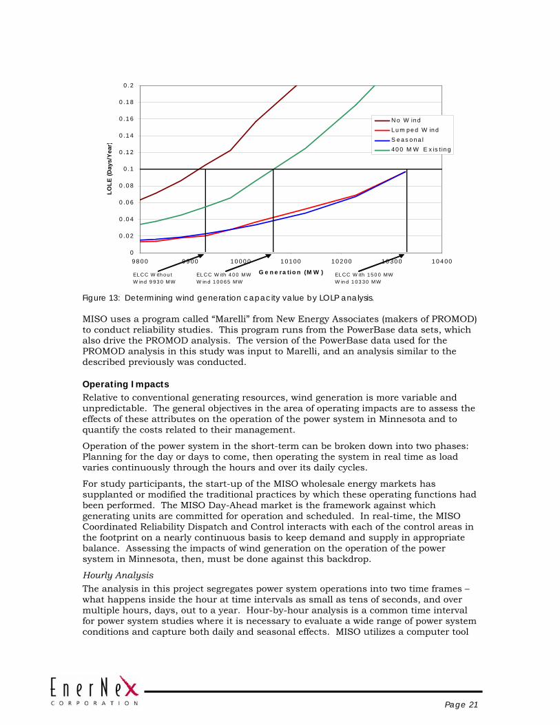
Page 21

0

0 .0 2

0 .0 4

0 .0 6

0 .0 8

0 . 1

0 .1 2

0 .1 4

0 .1 6

0 .1 8

0 . 2

9 8 0 0 9 9 0 0 10 0 0 0 1 0 1 0 0 1 0 2 0 0 1 0 3 0 0 1 0 4 00

G e n e ra tio n (M W )

LOLE

(Day

s/Y

ear)

N o W in dLu m pe d W in dS e a s o na l40 0 M W E x is t in g

EL CC W ith o u t W in d 9 9 3 0 MW

ELCC W ith 4 0 0 MW W in d 1 0 0 6 5 MW

EL CC W ith 1 5 0 0 MW W in d 1 0 3 3 0 MW

Figure 13: Determining wind generation capacity value by LOLP analysis.

MISO uses a program called “Marelli” from New Energy Associates (makers of PROMOD) to conduct reliability studies. This program runs from the PowerBase data sets, which also drive the PROMOD analysis. The version of the PowerBase data used for the PROMOD analysis in this study was input to Marelli, and an analysis similar to the described previously was conducted.

Operating Impacts Relative to conventional generating resources, wind generation is more variable and unpredictable. The general objectives in the area of operating impacts are to assess the effects of these attributes on the operation of the power system in Minnesota and to quantify the costs related to their management.

Operation of the power system in the short-term can be broken down into two phases: Planning for the day or days to come, then operating the system in real time as load varies continuously through the hours and over its daily cycles.

For study participants, the start-up of the MISO wholesale energy markets has supplanted or modified the traditional practices by which these operating functions had been performed. The MISO Day-Ahead market is the framework against which generating units are committed for operation and scheduled. In real-time, the MISO Coordinated Reliability Dispatch and Control interacts with each of the control areas in the footprint on a nearly continuous basis to keep demand and supply in appropriate balance. Assessing the impacts of wind generation on the operation of the power system in Minnesota, then, must be done against this backdrop.

Hourly Analysis The analysis in this project segregates power system operations into two time frames – what happens inside the hour at time intervals as small as tens of seconds, and over multiple hours, days, out to a year. Hour-by-hour analysis is a common time interval for power system studies where it is necessary to evaluate a wide range of power system conditions and capture both daily and seasonal effects. MISO utilizes a computer tool

Page 22

called PROMOD for this type of analysis. PROMOD contains representation of loads, transmission lines, and generating units. For the hourly load data provided as input, PROMOD determines the optimum plan for meeting the load while honoring constraints for the system (e.g. reserves, emissions, etc.) individual generating units, and the transmission network.

PROMOD can also be used to estimate locational marginal prices (LMP), since the cost functions and loading level of each generator in the optimized solution are known.

Intra-Hourly Analysis The hour-by-hour simulation in PROMOD assumes that load, wind, and generation are “flat” for each hour. In reality, load (and wind) is continuously varying, and provisions must be made by system operators for adjustments so that demand and supply are closely matched at all times.

An approach that has been used in previous studies for estimating the impact of wind generation on requirements for regulation, load following, and other reserve impacts is based on analysis of high resolution chronological wind and load data sets. Various statistical metrics that quantify variability are first computed for the load data alone. Wind data is then combined with load data, and new metrics are calculated. The changes in these quantities are directly attributable to wind generation.

Assessing the costs of these inside-the hour impacts has been done in a variety of ways. Direct costs, for example, can be computed for incremental regulation capacity if there is a regulation market or capacity cost that can be identified. However, if the incremental requirements for the various operating reserves are brought into the hourly analysis, much of the cost impact, especially those that are associated with opportunity cost, are accrued. A good example would be where regulation and load following is performed with relatively inexpensive units. The capacity that must be held back to provide ancillary services cannot be used to serve load and generate revenue. There is, therefore, an “opportunity” cost that comes with providing ancillary services from these units. The hourly modeling will accrue these costs since other resources must be used to meet the load.

Page 23

PROMOD(Hourly Analysis)

Mathematical &Statistical Analysis

GE-MARS(reliability analysis)

Hourly Load Data(2003,2004,2005

Hourly WindGeneration Data(2003,2004,2005)

NREL WindGeneration

MeasurementDatabase

5-minWind Generation

Data(partial 2005)

5-minLoad Data

( 2005)

NEA Marelli(Relability Analysis)

MISOPowerBase

MAPP/MRORSG StudyDatabase

Wind GenerationCapacity Value (ELCC);System Reliability

HOURLY ANALYSISMarket impactsLMP impactsEmissions reductionUnit commitment costsReserve costs

---- Analytical Tool---- MISO Data/Database---- Input Data---- Result/Output

Estimated Intra-HourlyImpacts

West RSGStudy Assumptions

Figure 14: Flowchart for Technical Analysis

STUDY DATA AND ASSUMPTIONS The MISO market and reliability footprints are comprised of thousands of individual generating units, many tens of thousands of megawatts of load, and many thousands of miles of transmission lines at or above 115 kV. Given the influence of the MISO energy market on the daily operations of the Minnesota companies, along with the geographical expanse of the wind generation to be considered, computer models to simulate generation scheduling and operations across the state of Minnesota must also be large.

MISO maintains large databases and computer models of network, load, and generator information to conduct a variety of regional studies. Some of these models cover the entire Eastern Interconnection (roughly all of the U.S. power system east of the Rocky Mountains). Others limit the detail to all or parts of the MISO footprint, and are used for transmission expansion planning studies.

For purposes of this study, the smaller models which represent a portion of the MISO footprint are most appropriate considering the level of detail desired.

Transmission issues for wind generation are not within the scope of this study. However, transmission capacity has a direct influence on the function of the wholesale energy market, as transmission losses and congestion are responsible for the differences in prices across the market footprint. An existing MISO planning model for PROMOD was selected as the starting point for this study. Figure 15 illustrates the

Page 24

scope of this West Regional Study Group (RSG) model created to encompass a number of separate transmission planning efforts so that they could be studied simultaneously.

WPL

ASEC

BREC, EKPC, TVA

IMO

KCPL

MIDAM

MIPU

MPC, NWPS, WAPA

STHRN

SWPA

ALWST

AUEP, CIPS, CIL

CGE, PSI

EEI

FE

GRE HUC

HEC

ILPC

IP&L

LG&E

MDU

MGE

CONS, DETED, LBWL, WPSC

MP

NIPS

NSP

OTP

SIGE

WEP

WPPI

WPS

SIPC, SPRIL

DPC

SMMPA

PJM, COED, AEP, DPL

MISO Market

LES, NPPD, OPPD

MPW

MHSP SASK

Figure 15: Overview of West RSG study PROMOD model, used as the basis for this study.

Companies shown in red are represented in detail.

The transmission and non-wind generation expansion assumptions in the MISO West RSG model were used because this study is focused on the reliability and operating impacts of wind generation and is not intended to be a transmission plan or an integrated resource plan. The wind generation in the RSG model was removed and replaced with the wind scenarios developed for this study. The makeup of the West RSG PROMOD model and assumptions underlying it are detailed in Appendix A

The size and makeup of an individual control area has a significant influence on its ability to manage wind generation. Currently there are several major control areas, or Balancing Authorities (BAs), in the state of Minnesota. MISO is currently well underway with the development of an Ancillary Services Market which will result consolidation of certain BA functions. This consolidation will decrease the aggregate amount of certain ancillary services.

Most of the transmission expansion in the model adapted for this study consists of additions to the existing EHV (extra high voltage, 345 kV or higher) network. The wind generation developed for the study is “injected” at EHV buses. This assumption is used by MISO in other studies where focus is on the larger picture, and bolstering of lower voltage transmission infrastructure is not part of the study scope. The underlying local and regional transmission infrastructure was not analyzed in this study

Page 25

Because the study year is more than a decade into the future, and the move toward functional consolidation of Balancing Authorities is already underway, the Minnesota companies will be considered as a single BA for the study. This could actually be a conservative assumption if after consolidation of BA’s in the MISO footprint the resulting regional BA is larger than Minnesota.

The PROMOD West RSG model, with the wind generation scenarios developed for this study, is used to represent the MISO energy market operations. It is assumed that this cost-based approach will adequately reflect the function of the day-ahead and real-time markets.

Modeling Minnesota Electric Load in 2020 Table 8 documents the retail sales statistics upon which the Minnesota study is premised. The total retail sales for 2004 were 61,965 GWH. Assuming a 2.0% annual growth rate, retail sales in 2020 are projected to be 85,093 GWH.

Table 8: Minnesota retail sales by company for CY2004 and Total Retail Sales assumptions for study

RetailSales Wind Wind

Annual Percent AnnualGrowth Retail CapacityRate Sales Factor 2004 2011 20201.0% MN Retail Sales (GWh) 61,986 66,457 72,683

15% 40% Nameplate wind (MW) 2,653 2,845 3,11120% 35% 4,043 4,335 4,74120% 40% 3,538 3,793 4,14925% 40% 4,422 4,741 5,186

2.0% MN Retail Sales (GWh) 61,986 71,202 85,09315% 40% Nameplate wind (MW) 2,653 3,048 3,64320% 35% 4,043 4,645 5,55120% 40% 3,538 4,064 4,85725% 40% 4,422 5,080 6,071

Table 9 shows the loads from the West RSG PROMOD case for 2020. The highlighted (in yellow) companies are those having significant Minnesota load. The aggregated load, however, for these companies is 142,177 GWH, well in excess of the study projections for 2020.

` 2004 MN RetailSales in kWh1

Investor-Owned UtilitiesXcel 30,559,280,490 49.3%MP 8,580,900,000 13.8%OTP 1,957,456,566 3.2%IPL 841,511,856 1.4%NWEC 524,992 0.0%

TOTAL IOU 41,939,673,904 67.7%

Cooperative UtilitesGRE 10,408,968,000 16.8%Minnkota 1,808,326,904 2.9%Dairyland 737,462,789 1.2%Basin 751,736,085 1.2%

TOTAL COOP 13,706,493,778 22.1%

Municipal UtilitiesSMMPA 2,714,070,325 4.4%MRES 805,570,000 1.3%MMPA 2,302,721,000 3.7%CMMPA 516,974,120 0.8%TOTAL MUNI 6,339,335,445 10.2%

TOTAL ALL 61,985,503,127 100.0%1 July 1, 2003 to June 30, 2004 (MN DOC 1/15/05)

Page 26

Table 9: Loads by Company from PROMOD West RSG case for 2020.

Company Load (MWH)ASEC 21195998GRE 19677281MDU 2807994MPC 7048485NWPS 1679993OTP 6843984WABDK 4445004ALWST 19728132AUEP 43335000MHSP 24793994SASK 20286020DPC 6675034HUC 408002MPL 12674090NSP 67017594SMMP 2512775LES 4328000MIDAM 25180996MPW 1133011NPPD 14662941OPPD 12225999WABNI 16423007COED 112141254CIL 7101042CIPS 20675055EEI 4322030ILPC 18021032SIPC 2019994SPRIL 2270002MGE 4038000WEP 37665970WPL 16316931WPPI 6069003WPS 15090049

A simple algorithm for extracting the Minnesota load from the PROMOD was utilized. From the work scope, the aggregated retail sales of five entities – Xcel Energy, Minnesota Power, Ottertail Power , Great River Energy, and SMMPA comprise 87.5% of Minnesota retail electricity sales. And, from 2004 data provided by MISO, it can be computed that the Minnesota portion of the Xcel-NSP load comprises 67% of their company load in MISO. Adjusting for the out-of-Minnesota sales for Xcel Energy, the load for these five entities from the PROMOD results is 86610 GWH.

To account for the other Minnesota companies listed in the table from the statement of work but not explicitly accounted for in the extraction from the PROMOD results, the aggregate load for the five companies is divided by 87.5%, yielding an estimated Minnesota state load of 98,983 GWH.

Page 27

The PROMOD load is not “retail sales” as it is comprised of the energy transported to high voltage delivery points (substations). Losses in the distribution system are estimated to be about 7%. Applying this factor to the PROMOD load to estimate “retail sales” at customer metering points yields estimated Minnesota retail sales of 92,054 GWH.

From information exchanged with MISO, it was confirmed that an average growth rate of 2.5% was assumed for scaling loads for the 2020 West RSG PROMOD case. The number above is almost identical to the 2004 Minnesota retail sales escalated at 2.5% annual growth to 2020. It appears, therefore, that the simple algorithm proposed does a good job in estimating Minnesota retail sales from the PROMOD data.

A consequence of the PROMOD loads in the 2020 West RSG case is that the wind generation data provided earlier amounts to slightly less than the target energy penetration levels due to slightly increased retail sales. After discussions, it was decided that the most straightforward way to compensate would be to increase the wind generation slightly. This was accomplished by increasing the installed capacity numbers by a factor equal to 92,054/86,610, or 1.063.

Correlated hourly wind generation and load data is a foundation for the hourly analysis in this study. Because wind generation and electric demand are both affected by the regional meteorology, it is important to preserve the correlations that might exist between these data sets. As previously described, chronological wind speed and generation data profiles were developed at five minute intervals for the historical years 2003, 2004, and 2005. To create the load data corresponding to these years, hourly load data from these years for the Minnesota companies was retrieved from archives and scaled per the discussion above to create load data for the study. CY2004 was selected as the “base” year in that it was modified to achieve the target annual retail electric sales. The ratio between the new peak hourly load for the 2020 data and the peak load for the historical 2004 load data was then applied to load data from 2003 and 2005.

Developing Wind Generation Data The basic approach for developing wind generation profiles is to apply a “power curve” from a commercial wind turbine to the wind speed values at each five-minute interval. With 152 observation points in the MM5 model and up to 6000 MW of wind generation potentially required in the model, each wind speed observation must represent more than a single turbine.

Appendix C describes the approach used for this study, which approximates spatial diversity, terrain, and turbine shadowing effects by adjusting raw wind speed values at high resolution before calculating power (Figure 16). Wind speed data at five-minute intervals over three consecutive calendar years across 152 separate locations across Minnesota and the eastern half of the Dakotas was processed to yield five-minute and hourly wind generation data for each of the scenarios.

In an earlier section and in the companion report, it was noted that net capacity factors were calculated by assuming a constant loss factor of 14%. The wind generation data calculated from the method described in the appendix makes no such assumption, as the effective plant power curve takes those factors which contribute to the losses into account.

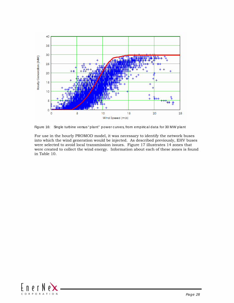
Page 28

Figure 16: Single turbine versus “plant” power curves, from empirical data for 30 MW plant

For use in the hourly PROMOD model, it was necessary to identify the network buses into which the wind generation would be injected. As described previously, EHV buses were selected to avoid local transmission issues. Figure 17 illustrates 14 zones that were created to collect the wind energy. Information about each of these zones is found in Table 10.

Page 29

Figure 17: Wind generation regions and network injection buses

Inje

ctio

n st

atio

ns

Tow

ers

to s

tatio

n

12

3

4

56

7

8

9

1011

1213

14

Page 30

Table 10: Meteorological Tower Assignments by Region and Scenario

Area Bus Voltage Towers MW – 15% MW – 20% MW – 25%

1 Forbes 500 kV 79, 80, 81, 82, 83, 84, 85 200 280 289

2 Winger 230 kV 63, 64, 133, 134, 138, 142, 143 200 280 280

3 Leland 345 kV 113, 114, 115, 116, 117, 123, 124, 125

280 320 320

4 Maple River 345 kV 2, 3, 91, 92, 126, 140, 141 240 280 280

5 Ellendale 230 kV 111, 112, 118, 119, 120, 121, 122 261 261 280

6 Alexandria 345 kV 10, 13, 65, 68, 88, 89, 127, 146, 147, 148

280 400 400

7 Watertown 345 kV 98, 99, 100, 101, 102, 103, 104, 105, 106, 109, 110

0 200 440

8 Granite Falls 345 kV 75, 78, 128, 129, 131, 135, 136, 137, 145, 150

360 400 400

9 Lyon County 345 kV 21, 22, 23, 24, 25, 26, 27, 28, 29, 30, 31, 32, 33, 34, 35, 50, 51, 52, 53, 54, 55, 67, 68, 69, 70, 71, 72, 73, 74, 93, 94, 95, 96, 97

607 767 1364

10 Adams 345 kV 38, 39, 40, 41, 42, 43, 44, 45, 139, 151

364 404 404

11 Willmarth 345 kV 8, 9, 11, 12, 86, 87, 130, 132, 144, 149, 152

283 443 443

12 Lakefield Jct. 345 kV 1, 4, 5, 6, 7, 14, 15, 16, 17, 18, 19, 20, 36, 37, 90

432 552 600

13 Nobles Co. 345 kV 46, 47, 48, 49, 56, 57, 58, 59, 60, 61, 62, 76, 77

127 207 520

14 Ft. Thompson 230 kV 107, 108 40 80 80

Total 3674 4874 6091

Page 31

Figure 18: Installed wind generation capacity by region and scenario

Figure 19: Wind energy production by region and scenario.

Table 11: Installed Capacity by Region and Penetration Scenario

Region 1

Region 2

Region 3

Region 4

Region 5

Region 6

Region 7

Region 8

Region 9

Region 10

Region 11

Region 12

Region 13

Region 14 Total

2004 15% 187 187 262 225 244 262 0 337 569 341 265 405 119 37 34412004 20% 263 263 301 263 245 376 188 376 721 380 417 519 195 75 45822004 25% 262 262 299 262 262 374 411 374 1274 377 414 560 486 75 5689

Adjusted Assignments of 2004 Wind Scenario Rationalized With MN 2004 Load Escalated to 2020

2004 Wind Energy By Region and Scenario

0

1000

2000

3000

4000

5000

6000

1 2 3 4 5 6 7 8 9 10 11 12 13 14Region Number

Win

d G

ener

atio

n (G

Wh)

25% Penetration20% Penetration15% Penetration

Allocation of Wind Capacity By Region and Scenario

0

200

400

600

800

1000

1200

1400

1 2 3 4 5 6 7 8 9 10 11 12 13 14Region Number

Win

d Ca

paci

ty

25% Penetration20% Penetration15% Penetration

Page 32

Table 12: Adjustment of Wind Generation Model to Achieve Study Target Penetrations

Target Energy Penetration

Derived Scale Factor

Wind Energy (GWh)

Actual Penetration

(Energy)15% 0.937 12715 14.97%20% 0.940 16953 19.96%25% 0.934 21192 24.95%

Target Retail Sales of 84922 GWh (based on 2004 adjusted 4 BA Loads)

Table 13: Characteristics of Wind Generation Model – Capacity Factor by Season & Region

Regions

Dakotas Buffalo Ridge

Central Minnesota

North Minnesota

South Minnesota

Total

`Winter 38.7% 43.9% 35.8% 32.7% 40.3% 39.2%

Spring 39.2% 43.3% 42.3% 40.6% 42.4% 42.1%

Summer 36.7% 40.1% 36.5% 38.8% 35.0% 37.8%

Autumn 45.8% 54.9% 48.2% 46.3% 51.1% 50.9%

Year 40.1% 45.6% 40.7% 39.6% 42.2% 42.7%

ESTIMATING RESERVE AND OTHER OPERATIONAL REQUIREMENTS Consideration of the controllable resources required to balance the control area and maintain security in PROMOD is handled by the “total operating reserve” setting for the balancing authority. The program will assure that this amount of capacity is available each hour and is not being used to serve load. This has the effect of extending the resource “stack”, and likely commits some more expensive resources.

For the MN balancing authority considered in this study, there are several categories of reserves:

• Regulating – capacity that can be adjusted up or down to maintain balance between control area demand and supply.

• Spinning – The extra amount of on-line generation capacity that must be carried to cover the largest contingency in the reserve sharing pool.

• Non-Spinning – an additional amount of generation that can be brought on-line in a short period of time to cover the largest contingency.

• Load Following – Capacity that can be adjusted up or down to follow the trend in the control area demand. This capacity will be economically dispatched at frequent intervals, and may include both generation participating in the MISO real-time market as well as regulating reserves.

Page 33

The baseline MISO assumption of 5% total operating reserves is larger than can be accounted for by summing the categories listed above. In the context of significant wind generation, this will include an amount of capacity to cover deviations from forecast conditions in the coming hour or hours. Such deviations would result from errors in short-term hourly load forecasts, for example. With significant amounts of wind generation in the control area, these additional reserves would be carried by operators to cover drops in wind generation over the next hour with respect to a persistence forecast.

Regulating Reserves Control area regulation is a capacity function. Compensation for load changes or deviations over very short time frames (tens of seconds to minutes) is provided by units capable of the necessary response rates and operating on Automatic Generation Control (AGC). As the size of a balancing authority increases, the regulation requirement as a fraction of the peak load generally declines. Such a relationship is depicted in Figure 20. This graph is based on conversations with operations personnel from MISO.

100 1 .103

1 .104

1 .105

0

0.02

0.04

0.06

0.08

0.1

0

100

200

300

400

500

Peak Load (MW)

Regu

latio

n C

apa

city

(% o

f pea

k lo

ad)

Regu

latio

n (M

W)

Figure 20: Approximate regulating requirements for a Balancing Authority as a function of peak

demand.

Using the relationship from Figure 20, regulation requirements for the existing Minnesota balancing authorities and the combined balancing authority in 2020 can be estimated. These are shown in Table 14. The effect of balancing authority functional consolidation is quite pronounced with regard to regulation requirements.

Page 34

Table 14: Estimated Regulating Requirements for Individual MN Balancing Authorities and Aggregate

Balancing Authority Peak Load Regulating

Requirement (from chart)

Regulating Requirement (% of peak)

GRE 3443 MW 56 MW 1.617%

MP 2564 MW 48 MW 1.874%

NSP 12091 MW 104 MW 0.863%

OTP 2886 MW 51 MW 1.766%

Sum of Regulating Capacity 259 MW

Combined 20984 MW 137 MW 0.655%

Fast changes in wind generation can increase the amount of regulation capacity required. Many previous studies have shown this impact to be quite modest, especially where the number of individual wind turbines relative to the system peak load is very high. The National Renewable Energy Laboratory (NREL) has been collecting high resolution data from operating wind plants for a number of years. Extensive analysis has been performed on this data that has contributed to the understanding of wind plant production variations on all operating time frames. Using the NREL measurement data, output fluctuations on the regulation time frame from a large wind plant are shown to be less than one or two percent of the plant nameplate rating (Figure 21).

Figure 21: Variation of the standard deviation of the regulation characteristic for each of nine

sample days by number of turbines comprising measurement group.

Page 35

Using a conservative estimate of 2 MW for each 100 MW of wind generation in the scenarios for this study, the regulation requirement for the combined MN balancing authority with the prescribed amounts of wind generation can be computed. By assuming that the regulation variations between each wind plant and the load are uncorrelated, the regulation requirement for the load and wind combination is computed with the following formula:

New_Regulating_Requirement k σLoad2 N σw100

2⎛⎝

⎞⎠⋅+:=

Where

k = a factor relating regulation capacity requirement to the standard deviation of the regulation variations; assumed to be 5

σLoad = standard deviation of regulation variations from the load

σw100 = standard deviation of the regulation variations from a 100 MW wind plant

N = wind generation capacity in the scenario divided by 100

Results of this computation for the three wind generation scenarios are shown in Table 15.

Table 15: Estimated Regulation Requirement for MN Balancing Authority in 2020

Scenario Regulation Capacity Requirement

Base 137 MW

15% Wind Generation 149 MW

20% Wind Generation 153 MW

25% Wind Generation 157 MW

Contingency Reserves The present reserve obligation for the Minnesota balancing authorities and companies is defined by the rules of the MAPP Generation Reserve Sharing Pool. The largest contingency which defines the pool’s reserve requirement is the loss of 1500 MW important from Manitoba on a 500 kV transmission line.

In the scenario defined for the study, the reserve obligation of the Minnesota utilities is projected to remain unchanged because:

• Loss of the Manitoba import is still assumed to be the largest single contingency

• The share of load in the reserve sharing pool, and the end-use load obligation (EULO) ratio of the Minnesota utilities to the larger pool is also assumed to remain the same.

Consequently, the Minnesota balancing authority would be required to carry 660 MW of reserve, of which 330 MW is spinning and 330 MW is quick-start.

Page 36

Note: After this study was well underway, the consolidation of the MAPP Generation Reserve Sharing Pool into a new, larger entity that largely encompasses the MISO Reliability Footprint was announced. The Midwest Contingency Reserve Sharing Group filed its participation agreement with the Federal Energy Regulatory commission in the fall of 2006. Beginning January 1, 2007, the Midwest contingency Reserve Sharing Group is scheduled to commence operations and is anticipated to reduce the contingency reserve obligation of the Minnesota utilities.

Load Following Within the hour, enough generation must be available to compensate for the underlying trends in the load beyond the fast regulation time frame. In MISO, load trends are accommodated by a combination of the real-time market and regulation capability. Either response cannot be directly considered in the PROMOD hourly analysis. Therefore, no distinction will be made, and the effects of wind generation will be gauged from analysis of load and wind time series data alone.

Figure 22 through Figure 24 depict the distributions of absolute changes over a five-minute interval for load and load net wind generation. The effect of wind generation on these changes is relatively modest, owing to the significant geographic diversity present in the wind scenarios.

Additional amounts of generic reserve can be estimated as some multiple of the standard deviations. As shown in Table 16, two standard deviations, which would encompass over 95% of all variations in the sample, was assumed. This assumption is consistent with operational practice for power systems. The metric by which control over periods of ten minutes is judged, CPS2 (Control Performance Standard 2) requires that the difference between load and generation over a ten-minute period must be smaller than a specified limit for 90% or more of the ten-minute intervals over the month. Consequently, not all deviations in the control area demand are fully compensated, as CPS2 scores for existing control areas vary across the range from 90 to 100%.

Table 16: Summary of Five-minute Variability

Scenario Standard Deviation of 5-minute changes

Base 50 MW

15% Wind Generation 55 MW

20% Wind Generation 57 MW

25% Wind Generation 62 MW

Page 37

0100020003000400050006000700080009000

10000

-250

-220

-190

-160

-130

-100 -7

0

-40

-10 20 50 80 110

140

170

200

230

Mor

e

Load Change (MW)

Occ

urre

nces

LoadNet Load W15

Load s = 50 MWNet Load s = 55 MW Bin Size 10 MWN = 79138

Figure 22: Five-minute variability – 15% wind generation

0

1000

2000

3000

4000

5000

6000

7000

8000

9000

10000

-250 -220 -190 -160 -130 -100 -70 -40 -10 20 50 80 110

140

170

200

230

More

Load Change (MW)

Occ

urre

nces

LoadNet Load W20

Load s = 50 MWNet Load s = 57 MW Bin Size 10 MWN = 79138

Figure 23: Five-minute variability – 20% wind generation

Page 38

0

1000

2000

3000

4000

5000

6000

7000

8000

9000

10000

-250 -220 -190 -160 -130 -100 -70 -40 -10 20 50 80 110

140

170

200

230

More

Load Change (MW)

Occ

urre

nces

LoadNet Load W25

Load s = 50 MWNet Load s = 62 MW Bin Size 10 MWN = 79138

Figure 24: Five-minute variability – 25% wind generation

Operating Reserve “Margin" The size and geographic diversity of the wind generation scenarios constructed for the study move the significant variability and uncertainty related to wind generation out to time frames ranging from one to several hours. Table 17 illustrates the standard deviation of the next-hour wind generation from a persistence forecast, which is a likely method for forecasting over such time frames. Distributions of next-hour errors from a persistence forecast are shown in Figure 25 through Figure 27.

The general response operationally to increased uncertainty in forward time frames is to carry additional reserves. How specifically this would be done in some optimal fashion for wind generation is not yet known. Some control area operators pad their reserves by an amount proportional to what they consider the next hour uncertainty due to load forecast to be. Within this MISO centralized dispatch structure, it is not clear how a large state-wide balancing authority would cover unexpected deviations (especially reductions) in wind generation. However, because of the size and diversity of the wind generation scenarios, nearly all of the significant impacts on variability and operational uncertainty are outside of the hour. Therefore, an operating reserve margin to cover unpredictable changes in wind generation from hour to hour is a conservative, yet reasonable approximation. For purposes of this study, additional reserve in the amount of two times the standard deviation will be assumed.

Table 17: Next-hour Deviation from Persistence Forecast by Wind Generation Scenario

Scenario Standard Deviation of 1-hour Wind Generation Change

15% Wind Generation 155 MW

20% Wind Generation 204 MW

25% Wind Generation 269 MW

Page 39

0

500

1000

1500

2000

2500

3000

-100

0

-900

-800

-700

-600

-500

-400

-300

-200

-100 0

100

200

300

400

500

600

700

800

900

1000

Hourly Delta (MW)

Cou

ntsigma = 155 MWBin Size - 25 MWN = 26301

Figure 25: Next-hour deviation from persistence forecast – 15% wind generation

0

500

1000

1500

2000

2500

-100

0

-900

-800

-700

-600

-500

-400

-300

-200

-100 0

100

200

300

400

500

600

700

800

900

1000

Hourly Delta (MW)

Cou

nt

sigma = 204 MWBin Size - 25 MWN = 26301

Figure 26: Next-hour deviation from persistence forecast – 20% wind generation

Page 40

0

200

400

600

800

1000

1200

1400

1600

1800

2000

-100

0

-900

-800

-700

-600

-500

-400

-300

-200

-100 0

100

200

300

400

500

600

700

800

900

1000

Hourly Delta (MW)

Cou

ntsigma = 269 MWBin Size - 25 MWN = 26301

Figure 27: Next-hour deviation from persistence forecast – 25% wind generation

Analysis of the load and wind generation time series data reveals that the significant effects of wind generation on the operation of the Minnesota Balancing Authority are actually outside the hour, i.e. there are only modest impacts on time frames associated with regulation or the real-time market. Consequently, the additional amounts of reserve capacity for these services would also be modest.

Based on the assumptions discussed with the TRC, the spinning and non-spinning reserve requirements for the Minnesota balancing authorities and companies would not be affected by the presumed consolidation into a single balancing authority.

Covering unanticipated changes in wind generation over periods of an hour or more appears to be the area where wind generation would have the largest impact. By considering some additional amount of reserves to cover this uncertainty, and factoring in the incremental requirements from the other categories, the “Total Operating Reserve” criteria for the PROMOD studies can be developed for the three wind generations scenarios. These estimates, in MW and as a percentage of the balancing authority peak load, are shown in Table 18.

Discussion The need for additional reserves beyond those identified for regulation and load following was discussed extensively with the TRC.

A plan for the PROMOD cases was developed to assess the degree to which reserve assumptions would affect integration costs. Cases for the 5% operating reserves roughly correspond to the situation where the “operating reserve margin” from Table 18 is zero for all wind generation scenarios (due to the fact that wind generation has only minor impacts on the within-the hour reserves from the data analysis). Three new cases for the base year of 2004 and each wind generation penetration level were run with the total operating reserves as specified in Table 18. Sensitivity cases were run around each of these three new cases where the reserve requirement 1% higher and 1% lower than the value from the table to assess the cost sensitivity to operating reserve assumptions. This sensitivity is discussed later in the report.

Page 41

Table 18: Estimated Operating Reserve Requirement for MN Balancing Authority – 2020 Load

Base 15% Wind 20% Wind 25% Wind Reserve Category MW % MW % MW % MW %

Regulating 137 0.65% 149 0.71% 153 0.73% 157 0.75% Spinning 330 1.57% 330 1.57% 330 1.57% 330 1.57% Non-Spin 330 1.57% 330 1.57% 330 1.57% 330 1.57% Load Following 100 0.48% 110 0.52% 114 0.54% 124 0.59% Operating Reserve Margin 152 0.73% 310 1.48% 408 1.94% 538 2.56% Total Operating Reserves 1049 5.00% 1229 5.86% 1335 6.36% 1479 7.05%

Notes on Table:

• Assumes 2020 MN Balancing Authority peak load of 20984 MW

• Requirements for load following and reserve margin based on two standard deviations of the five-minute variability and next hour forecast error, respectively.

MODELING TIME-VARYING RESERVE REQUIREMENTS IN PROMOD PROMOD is generally capable of modeling only a constant operating reserve level for a single case. New Energy Associates provided guidance on a work-around for varying the operating reserves by hour.

A variable operating reserve level is created by introducing a fictitious generating resource that is dedicated to serving a fictitious load. The available capacity on the resource is counted toward the total operating reserves in the balancing area of interest. By varying the load served by the fictitious resource, the available capacity and hence the reserve contribution can be varied by the profile of the fictitious load.

Wind generation data for each scenario was analyzed to characterize the variability over one hour. Figure 28 shows plots of the wind generation changes over a single hour for each scenario. Of interest is the revelation that the maximum variability does not occur at maximum generation, but rather in the mid-range of the aggregate production curve.

Standard deviations for each quintile of production were computed for the samples above, and are documented in Table 19. To facilitate modeling a time-varying reserve profile, quadratic approximations to the empirical curves were developed (Figure 29). With these quadratic expressions, an hourly profile for this operating reserve margin was developed for PROMOD from the hourly wind generation data.

The time-varying reserve profile is illustrated in Figure 30 for six weeks of hourly data. The statistics of the varying reserve profile used in this study are documented in Table 20. The average value over the year is smaller than the “fixed reserve” assumption, although there are hours where there is much more reserve being carried, as evidenced by the peak values.

Page 42

2000 1500 1000 500 0 500 1000 1500 20000

1000

2000

3000

4000

5000

6000

Hourly Change (MW)

Prod

uctio

n Le

vel (

MW

)

2000 1500 1000 500 0 500 1000 1500 20000

1000

2000

3000

4000

5000

6000

Hourly Change (MW)

Prod

uctio

n Le

vel (

MW

)

2000 1500 1000 500 0 500 1000 1500 20000

1000

2000

3000

4000

5000

6000

Hourly Change (MW)

Prod

uctio

n Le

vel (

MW

)

Figure 28: Hourly wind generation changes as functions of production level. 15% (left); 20%

(middle); 25% (right)

Table 19: Standard Deviation of One-Hour Production Changes by Generation Level

One Standard Deviation of 1-Hour Power Change

15% Wind (3441 MW) 20% Wind (4582 MW) 25% Wind (5689 MW)

Production Level

MW % MW % MW %

0 – 20% 103 2.88% 155 3.38% 177 3.11%

20% - 40% 178 5.11% 249 5.43% 314 5.52%

40$ - 60% 201 5.84% 249 5.43% 352 6.19%

60% - 80% 176 5.11% 194 4.23% 306 5.38%

80% - 100% 105 3.05% 135 2.95% 173 3.04%

Average 156 4.53% 205 4.47% 269 4.73%

Page 43

0 1000 2000 3000 4000 5000 60000

100

200

300

400

15%20%25%

15%20%25%

Wind Generation Level

StD

ev o

f 1-H

our P

ower

Cha

nge

0 1000 2000 3000 4000 5000 60000

100

200

300

400

f25 xi⎛

⎝⎞⎠

f20 xi⎛

⎝⎞⎠

f15 xi⎛

⎝⎞⎠

xi

f15 x( ) 200x 2000−( )

2

18000−:=

f20 x( ) 275x 2800−( )

2

30000−:=

f25 x( ) 350 1x 3500−( )

2

35000−:=

Figure 29: Empirical next-hour wind variability curves (top) and quadratic approximation (middle)

and equations (bottom). Vertical axis quantity on charts is standard deviation.

Page 44

150 151 152 153 154 155 156 157 158 159 160 161 162 163 1640

1000

2000

3000

4000

5000

6000

0

2000

4000

6000

Day

Win

d G

ener

atio

n (M

W)

Ad

diti

onal

Res

erve

(MW

)

150 151 152 153 154 155 156 157 158 159 160 161 162 163 1640

1000

2000

3000

4000

5000

6000

0

1000

2000

3000

4000

5000

6000

Day

Win

d G

ener

atio

n (M

W)

Ad

diti

onal

Res

erve

(MW

)150 151 152 153 154 155 156 157 158 159 160 161 162 163 1640

1000

2000

3000

4000

5000

6000

0

1000

2000

3000

4000

5000

6000

Day

Win

d G

ener

atio

n (M

W)

Ad

diti

onal

Res

erve

(MW

)

Figure 30: Illustration of time varying “operating reserve margin” developed from statistical

analysis of hourly wind generation variations.

Operating reserve margin

Page 45

Table 20: Characteristics of Additional Variable Reserve

Additional Variable Reserve

15% Wind (3441 MW) 20% Wind (4582 MW) 25% Wind (5689 MW) Characteristic MW % of

System Peak MW % of

System Peak MW % of

System Peak

Mean 259 1.23% 384 1.83% 473 2.25%

Maximum 400 1.91% 550 2.62% 700 3.34%

Page 46

Section 4 RELIABILITY IMPACTS

The goal of the reliability analysis is to determine the capacity value of wind generation at each penetration level. The reliability impacts scope from the statement of work for the project is as follows:

The base model for this study was adapted from the West RSG generation and transmission expansion assumptions. The new conventional generating capacity is shown in Figure 31.

The West RSG case focuses on a 2011 study year, so the assumed loads for this study are higher.

Evaluate the reliability impacts of the wind generation in the planning horizon (seasonal and annual, for three years):

• Determine the impact of the wind generation on regional reliability (Loss of Load Probability) and reserve capacity obligations.

• Determine the capacity value of the wind generators by calculating their effective load carrying capability (ELCC) to measure the wind plant’s capacity contributions based on its influence on overall system reliability; review and discuss inter-annual variations in ELCC; evaluate simplified methods of approximating ELCC.

• Compare results to the existing MAPP guidelines for establishing capability ratings for variable capacity generation and develop recommendations for improvements to the guidelines. Model and Input Data:

It is anticipated that reliability impacts analysis can be developed from the GE Multi-Area Reliability Simulation (MARS) program and the associated database developed for the recent MAPP Reserve Capacity Obligation Review with both thermal and hydro resources included.

Page 47

biomass, 15 MW

Wind, 2933 MW

Natural Gas, 300 MW

Coal, 2861 MW

Coal and/or a blend of Petroleum coke and

coal, 580 MW

Figure 31: New conventional generation in West RSG expansion plan

An initial assessment of wind energy production during the highest system load hours is presented in Figure 32. Three years of wind and load data (2003, 2004, and 2005) are sorted in descending order by load. Wind generation for the highest load hours is then summed, and the capacity factor for that number of hours is computed as an estimate of the contribution to system reliability.

An initial assessment of the capacity value of wind generation can be made with chronological wind and load data only. High load hours generally represent times when the system could be at risk of not having sufficient generation to meet demand. While these peak load hours may not represent the only times when the system is “at risk”, they are the major considerations for capacity planning studies.

Focusing only on the peak hours ignores the characteristics of the conventional generation portfolio, and assumes that load level is the only indicator of system reliability risk. It is, however, much less intensive in terms of data and computing time, and has been shown to provide an indication of the relative capacity contribution of wind generation in a particular system context.

The mathematical procedure is straightforward:

1. Construct a 2 x 8760 matrix, where the first column is hourly load and the second is hourly wind generation.

2. Sort the matrix of hourly load and wind generation pairs by the hourly load value, in descending order.

3. Calculate the wind energy delivery for the x highest load hours

4. Divide the wind energy delivered over those hours by the maximum that could have been delivered (installed capacity times number of hours)

5. Plot the results for various values of x.

Results of this procedure for each wind generation and load pattern year are shown in Figure 32.

Page 48

GE-MARS ANALYSIS The data set developed for the most recent MAPP Reserve Capacity Obligation (RCO) review was updated to reflect the assumptions for this study. The new generation capacity per Figure 31 was added, using forced outage data from similar units already in the data set. Hourly loads in the Minnesota area were replaced by those developed for this study. Loads in other areas were scaled by the same factor used to develop the 2020 loads for Minnesota.

Wind is treated as a load modifier. This involves running two separate cases – one with load alone (no wind), and the other with the hourly loads net of wind generation. All three sets of wind and load patterns corresponding to calendar years 2003, 2004, and 2005 were used.

A significant amount of new capacity in the Minnesota area was required to bring the reliability level to the target 1 day in 10 years for the no wind case. This shows that the baseline generation expansion assumptions for the study would not provide adequate reliability for projected 2020 loads.

Results Results of the GE-MARS simulations are presented in Figure 33 through Figure 35 and Table 21 through Table 23.

Page 49

1 10 100 1 .1030.2

0.36

0.52

0.68

0.84

1

15%20%25%

15%20%25%

2003 Wind and Load Patterns

# of Hours (1-year period)

Cap

acity

Fac

tor (

pu)

1 10 100 1 .1030

0.2

0.4

0.6

0.8

1

15%20%25%

15%20%25%

2004 Wind and Load Patterns

# of Hours (1-year period)

Ca

paci

ty F

act

or (p

u)

1 10 100 1 .1030

0.2

0.4

0.6

0.8

1

15%20%25%

15%20%25%

2005 Wind and Load Patterns

# of Hours (1-year period)

Ca

paci

ty F

act

or (p

u)

Figure 32: Wind generation capacity factor for varying number of highest load hours. (2003, 2004,

and 2005 wind and load patterns)

Page 50

0

0.1

0.2

0.3

0.4

0.5

0.97 0.98 0.99 1 1.01 1.02 1.03 1.04 1.05 1.06 1.07 1.08

Load (pu)

LOLE

2003 Base2003 15%2003 20%2003 25%

Figure 33: LOLE for Minnesota Area based on 2003 load and wind patterns

0

0.1

0.2

0.3

0.4

0.5

0.97 0.98 0.99 1 1.01 1.02 1.03 1.04 1.05 1.06

Load (pu)

LOLE

2004 Base2004 15%2004 20%2004 25%

Figure 34: LOLE for Minnesota Area based on 2004 load and wind patterns

0

0.1

0.2

0.3

0.4

0.5

0.97 0.98 0.99 1 1.01 1.02 1.03 1.04 1.05 1.06

Load (pu)

LOLE

2005 Base2005 15%2005 20%2005 25%

Figure 35: LOLE for Minnesota Area based on 2005 load and wind patterns

Page 51

Table 21: ELCC Results for 2003 Wind and Load Patterns

Wind Penetration

ELCC (pu)

Peak Load (MW)

ELCC (MW)

Wind (MW)

ELCC (%)

15% 0.046 15630 719 3441 20.9%

20% 0.059 15630 922 4582 20.1%

25% 0.062 15630 969 5688 17.0%

Table 22: ELCC Results for 2004 Wind and Load Patterns

Wind Penetration

ELCC (pu)

Peak Load (MW)

ELCC (MW)

Wind (MW)

ELCC (%)

15% 0.026 15630 406 3441 11.8%

20% 0.035 15630 547 4582 11.9%

25% 0.041 15630 641 5688 11.3%

Table 23: ELCC Results for 2005 Wind and Load Patterns

Wind Penetration

ELCC (pu)

Peak Load (MW)

ELCC (MW)

Wind (MW)

ELCC (%)

15% 0.01 15630 156 3441 4.5%

20% 0.015 15630 234 4582 5.1%

25% 0.015 15630 234 5688 4.1%

Discussion Variation in ELCC between years is maybe the most surprising aspect of the results. Both load and wind patterns vary by year, and correspond to the meteorological conditions for those years. Results for calendar year 2003 wind and load patterns is in the range of what might have been expected from those who have been engaged in the wind capacity value discussion. In the other years, it is significantly lower.

The trend in the ELCC by year is consistent with what was found from the analysis of wind and load data only, in that 2003 shows the best correlation between wind production during the highest load hours, with 2005 exhibiting the poorest correlation. This is evident from the capacity factor over the highest load hours as shown in Figure 32. Examining hourly wind energy delivery for the highest load hours of each calendar year (Figure 36), rather than cumulative production as in Figure 32 provides an even better view. It is apparent from the plots that wind production was much lower during the highest load hours in 2005, especially in the highest 40 hours. In 2003, on the

Page 52

other hand, there was significant generation during those same hours, with 2004 somewhere between.

0 10 20 30 40 50 60 70 80 90 1000

0.10.20.30.40.50.60.70.80.9

1CY2003

Hour (sorted by load)

Win

d G

ener

atio

n (p

u)

0 10 20 30 40 50 60 70 80 90 1000

0.10.20.30.40.50.60.70.80.9

1CY2004

Hour (sorted by load)

Win

d G

ener

atio

n (p

u)

0 10 20 30 40 50 60 70 80 90 1000

0.10.20.30.40.50.60.70.80.9

1CY2005

Hour (sorted by load)

Win

d G

ener

atio

n (p

u)

Figure 36: Hourly wind production for highest 100 load hours of year (20% scenario)

Page 53

RESULTS FROM MARELLI Marelli runs performed by MISO also show that the new capacity in the West RSG assumptions is not sufficient for the 2020 loads developed for this study. The same observation was made during the MARS analysis, but in those cases additional capacity was added to the Minnesota area to bring the reliability without wind generation to the target level. No such modification was made to the data for the initial Marelli analysis.

Results from the initial Marelli cases are shown graphically in Figure 37 through Figure 39.

2003 Data LOLP

20002100220023002400250026002700280029003000310032003300340035003600370038003900400041004200

0 0.1 0.2 0.3 0.4 0.5 0.6 0.7 0.8 0.9 1

LOLP

Add

ition

al C

apac

ity (M

W)

No Wind 15% Wind 20% Wind 25% Wind

The capacity scale on the Y-axis represents the base resource availability at y=0, while the increasing capacity demonstrates affects of imports on the system LOLP.

Figure 37: LOLH (Loss of Load Hours) from Marelli analysis for 2003 wind and load patterns

Page 54

2004 Data LOLP

500

600

700

800

900

1000

1100

1200

1300

1400

1500

1600

1700

1800

1900

2000

2100

2200

0 0.1 0.2 0.3 0.4 0.5 0.6 0.7 0.8 0.9 1

LOLP

Add

ition

al C

apac

ity (M

W)

No Wind 15% Wind 20% Wind 25% Wind

The capacity scale on the Y-axis represents the base resource availability at y=0, while the increasing capacity demonstrates affects of imports on the system LOLP.

Figure 38: LOLH (Loss of Load Hours) from Marelli analysis for 2004 wind and load patterns

2005 Data LOLP

3000

3100

3200

3300

3400

3500

3600

3700

3800

3900

4000

4100

4200

4300

4400

4500

0 0.1 0.2 0.3 0.4 0.5 0.6 0.7 0.8 0.9 1

LOLP

Add

ition

al C

apac

ity (M

W)

No Wind 15% Wind 20% Wind 25% Wind

The capacity scale on the Y-axis represents the base resource availability at y=0, while the increasing capacity demonstrates affects of imports on the system LOLP.

Figure 39: LOLH (Loss of Load Hours) from Marelli analysis for 2005 wind and load patterns

To allow for a more direct comparison, MARS cases were re-run to more closely match the assumptions used in the analysis by MISO. These are shown in Figure 40 through Figure 42.

A comparison of the ELCC results obtained from the GE-MARS and Marelli LOLP analysis is provided in Table 24.

Page 55

0

0.1

0.2

0.3

0.4

0.5

0.97 0.98 0.99 1 1.01 1.02 1.03 1.04 1.05 1.06 1.07 1.08 1.09 1.1Load (pu)

LOLE

2003 Base2003 15%2003 20%2003 25%

Figure 40: GE-MARS results for isolated MN system; 2003 wind and load patterns

0

0.1

0.2

0.3

0.4

0.5

0 .97 0.98 0.99 1 1.01 1 .02 1.03 1.04 1 .05 1.06

L o a d (p u )

LOLE

2004 B as e2004 15%2004 20%2004 25%

Figure 41 GE-MARS results for isolated MN system; 2004 wind and load patterns

0

0.1

0.2

0.3

0.4

0.5

0.97 0.98 0.99 1 1.01 1.02 1.03 1.04 1.05 1.06

Loa d (pu)

LOLE

2005 Base2005 15%2005 20%2005 25%

Figure 42: GE-MARS results for isolated MN system; 2005 wind and load patterns

Page 56

Table 24: Comparison of ELCC Results from GE-MARS and Marelli LOLP Analysis

2003 Load Shape ELCC Analysis for Minnesota Load

GE-MARS Results

pu dELCC Peak Load dELCC MW Wind % ELCC 15% 0.061 15630 953 3441 27.7% 20% 0.071 15630 1110 4582 24.2% 25% 0.081 15630 1266 5688 22.3%

Marelli Results

2003 Load Shape ELCC Analysis for Minnesota Load

Cap Add (mw) Base Cap Add (mw) dELCC MW Wind % ELCC

15% 3050 4100 1050 3441 30.5% 20% 2900 4100 1200 4582 26.2% 25% 2825 4100 1275 5688 22.4%

2004 Load Shape ELCC Analysis for Minnesota Load

GE-MARS Results

pu dELCC Peak Load dELCC MW Wind % ELCC 15% 0.029 15630 453 3441 13.2% 20% 0.039 15630 610 4582 13.3% 25% 0.043 15630 672 5688 11.8%

Marelli Results

2004 Load Shape ELCC Analysis for Minnesota Load

Cap Add (mw) Base Cap Add (mw) dELCC MW Wind % ELCC

15% 1350 2000 650 3441 18.9% 20% 1260 2000 740 4582 16.2% 25% 1200 2000 800 5688 14.1%

2005 Load Shape ELCC Analysis for Minnesota Load

GE-MARS Results

pu dELCC Peak Load dELCC MW Wind % ELCC 15% 0.012 15630 188 3441 5.5% 20% 0.017 15630 266 4582 5.8% 25% 0.02 15630 313 5688 5.5%

Marelli Results

2005 Load Shape ELCC Analysis for Minnesota Load

Cap Add (mw) Base Cap Add (mw) dELCC MW Wind % ELCC

15% 3850 3980 130 3441 3.8% 20% 3835 3980 145 4582 3.2% 25% 3820 3980 160 5688 2.8%

Page 57

DISCUSSION When run using the same wind generation and load patterns, and the same assumptions for modeling of the Minnesota power system, the ELCC results obtained through LOLP analysis with both GE-MARS and Marelli are consistent. Further support is obtained by analyzing more detailed output from the programs which indicates the weeks of the year from the respective simulations where generation was insufficient to meet load in the statistical trials. This output is shown in Figure 43 through Figure 45 for each pattern year, and requires some explanation.

The vertical axes on the charts represent different quantities; the time scale, however is synchronized. For each year it can be seen that the system was at some risk during the same periods. Even though the programs utilize different algorithmic approaches for the LOLP analysis, they both show that the combination of wind generation, load, maintenance outages, etc. during certain periods can result in loss of load if forced generation outages should occur

Figure 43: Weekly LOLP results for 2003 for GE-MARS and Marelli

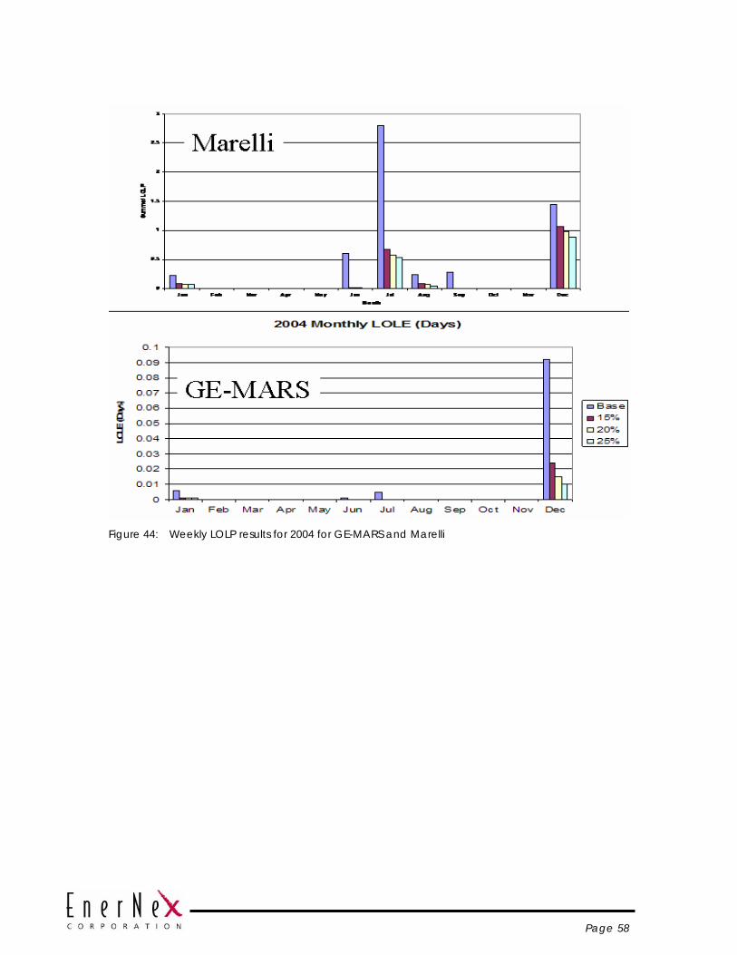
Page 58

Figure 44: Weekly LOLP results for 2004 for GE-MARS and Marelli

Page 59

Figure 45: Weekly LOLP results for 2005 for GE-MARS and Marelli

The numerical results from the LOLP analysis are slightly lower than the capacity accreditation as determined by the existing MAPP Reserve Sharing Group policy for accrediting intermittent generation. This policy was first developed for small hydro systems, and uses an after-the-fact accounting procedure based on the amount of energy deliveries during a four hour window around the monthly peak hour. It is specified to be applied over a ten-year rolling window, so the monthly accredited capacity is actually the median value of the monthly samples over the previous decade.

Table 25 shows the results of applying the MAPP Generation Reserve Sharing Pool (GRSP) accreditation procedure to the wind model developed for this study. Of note are the accredited capacity values during the summer peak season, the months of July and August. These are median values from the peak period window over the three years. Unlike the LOLP analysis, all deliveries in the four hour window around the monthly peak hour are counted, even if the peak load for the month is significantly lower than would be expected. This was the case for 2004, where the peak actually occurred in the winter. Additionally, the MAPP methodology makes no distinction between days during the month. Over a period of a few days leading up to the monthly peak hour, wind generation may be low. As is often the case in the Great Plains, hot spells are broken

Page 60

by frontal passages that can bring vigorous winds. High wind generation during these periods also affects the statistic.

Table 25: Capacity Accreditation of Wind Generation for Study per MAPP RSG Methodology

MW% of Wind MW

% of Wind MW

% of Wind

Jan 793 23% 1094 24% 1353 24%Feb 783 23% 1034 23% 1231 22%Mar 1261 37% 1661 36% 2056 36%Apr 1503 44% 2032 45% 2557 45%May 1674 49% 2215 48% 2743 48%Jun 902 26% 1185 26% 1416 25%Jul 715 21% 951 21% 1167 21%Aug 674 20% 904 20% 1087 19%Sep 1251 36% 1687 37% 2111 37%Oct 1052 31% 1401 31% 1731 30%Nov 1346 39% 1793 39% 2319 41%Dec 1442 42% 1928 42% 2450 43%

15% Penetration 20% Penetration 25% Penetration

SUMMARY A variety of methods were employed to assess the contribution of the wind generation model developed for this study to the reliability of the Minnesota power system. The results were consistent across all of the methods, and show that the effective capacity of wind generation can vary significantly year-to-year. The ELCC of the wind generation corresponding to 15% to 25% of Minnesota retail electric sales ranges from approximately 5% to just over 20% of nameplate capacity.

Meteorological conditions are the most likely explanation for this variation, as it can affect both electric demand and wind generation. The historical years used as the basis for this study did exhibit some marked differences attributable to weather, especially in 2004 where the annual peak actually occurred in the winter, rather than in the late summer months as is the norm.

Capacity value as computed through a rigorous LOLP analysis, along with the average number derived with such methods as that utilized by the MAPP GRSP can be expected to improve and converge as more years of data are added to the sample.

Page 61

Section 5 OPERATING IMPACTS

OVERVIEW In the operating time frame – hours to days – wind generation and load follow different cycles. Load exhibits a distinct diurnal pattern through all seasons. Wind generation in the Great Plains exhibits some diurnal characteristics, but is mainly driven by the passage of large scale weather systems that have cycles of several days to a week. It is nearly impossible, therefore, to select a small number of “typical” wind and load days for analysis.

The approach first used in the study for Xcel Energy in 2004 overcomes this difficulty by utilizing synchronized historical load and wind generation data sets extending over several years. Correlations due to the common meteorology are automatically embedded in these records, and a much wider range of combinations of wind generation and load behavior are represented. With multiple annual data sets, inter-annual variations in the meteorology can be captured.

With these data sets as the starting point, assessment of wind integration issues can be accomplished through a “simulation” of operational activities. For most utilities, this involves a forward-looking process where resources are committed for operation based on forecasts of load and wind. The selected resources are then dispatched against the “actual” load and wind generation to simulate real-time operations. Using planning tools that operate on time steps of one hour, an entire annual set of wind and load data can be processed.

MISO utilizes PROMOD for hour-by-hour analysis of energy market operations and transmission facility utilization. In this program, generating units are committed based on costs, operating characteristics, and transmission constraints, then dispatched to meet the specified load on an hourly basis. Like other hourly production costing programs, it can be used as a “proxy” for the short-term operation of power systems.

In this study, PROMOD is utilized to simulate the operation of the MISO energy markets. Annual data sets of wind generation and load developed from synthesized and historical data for calendar years 2003, 2004, and 2005 are the primary inputs to the program. System characteristics, such as transmission network data and generating unit costs and capabilities, are drawn from the database that MISO utilizes for transmission planning studies.

“BASE” CASES The initial PROMOD cases utilized the Minnesota load patterns from 2004 scaled to 2020 levels, and wind generation from the same year. Wind generation was injected at 14 buses in Minnesota and the Dakotas, and treated as a “firm” transaction. PROMOD uses firm transactions in the unit commitment step of the simulation, so the results represent an optimized commitment and dispatch for the entire year.

Page 62

Output from the PROMOD analysis can include the hourly profile of load at any bus, flows in any line, or output from any generator. The results presented here and throughout this section are based on summary information, and consist of the following quantities:

• Load – The annual energy consumed by end-users in the Minnesota company footprints in the PROMOD case. The target Minnesota retail electric energy sales are based on load patterns from 2004. Units are terawatt-hours (TWH), which is 1 million MWH.

• Wind Generation – Annual energy delivered by the wind generation in the scenarios constructed for this study. The amount varies by year, with target fraction of retail electric energy sales for wind based on meteorology from the year 2004. Units are terawatt-hours (TWH), which is 1 million MWH.

• Generation (non-wind) – Annual electric energy production from conventional generating resources. Units are terawatt-hours (TWH), which is 1 million MWH.

• Load Cost – The annual amount paid by the loads for the electric energy consumed. This quantity is equal to the summation over all hours of the year and all utilization buses in the Minnesota companies’ PROMOD footprints of the hourly amount at each utilization bus times the hourly locational marginal price at that utilization bus. Units are in millions of dollars.

• Production Cost – Variable costs associated with electric energy production. Includes fuel, startup and shutdown, and O&M costs. This amount does not include any consideration for capital recovery. Units are in millions of dollars.

• Generator Revenue – The annual amount paid to the generators. This quantity is equal to the summation over all hours of the year and all delivery buses in the Minnesota companies’ PROMOD footprints of the hourly amount at each delivery bus times the hourly locational marginal price at that delivery bus. Units are in millions of dollars.

• Imports – The amount of energy utilized by loads in the Minnesota companies’ PROMOD footprint but produced outside of that footprint. Units are terawatt-hours (TWH), which is 1 million MWH.

The case was run multiple times for different operating reserve assumptions to generate a curve for each wind generation level. Production costs and load payments are shown in Figure 46 and Figure 47. The effect on the utilization of conventional generation is shown in Figure 48 and Figure 49.

These optimized hourly cases show the following impacts of wind generation:

• As more wind energy is added, the production cost and load payments decline. This is due to the displacement of conventional generation and the resulting reduction in variable (fuel) costs.

• Generation from both coal and gas units is displaced.

• Production costs rise with the level of required operating reserves. This is intuitive, since more generation must be available or online.

• Production costs rise slowly from the baseline assumption of 5% total operating reserves out to about 7%. From there, costs rise more quickly.

Page 63

• As the operating reserve requirement is increased, coal units are further displaced in favor of more flexible gas units.

Minnesota Companies Production Cost

$1,880,000,000

$1,890,000,000

$1,900,000,000

$1,910,000,000

$1,920,000,000

$1,930,000,000

$1,940,000,000

$1,950,000,000

$1,960,000,000

$1,970,000,000

$1,980,000,000

4% 5% 6% 7% 8% 9% 10% 11% 12% 13%

Operating Reserve Margin

Pro

duc

tion

Co

st

15% wind20% wind25% wind

Figure 46: Production cost for Minnesota companies as a function of wind penetration and

operating reserve level.

Page 64

Minnesota Companies Load Cost

$3,650,000,000

$3,700,000,000

$3,750,000,000

$3,800,000,000

$3,850,000,000

$3,900,000,000

4% 5% 6% 7% 8% 9% 10% 11% 12% 13%

Operating Reserve Margin

Loa

d P

aym

ents

15% wind20% wind25% wind

Figure 47: Load payments for Minnesota companies as a function of wind penetration and

operating reserve level.

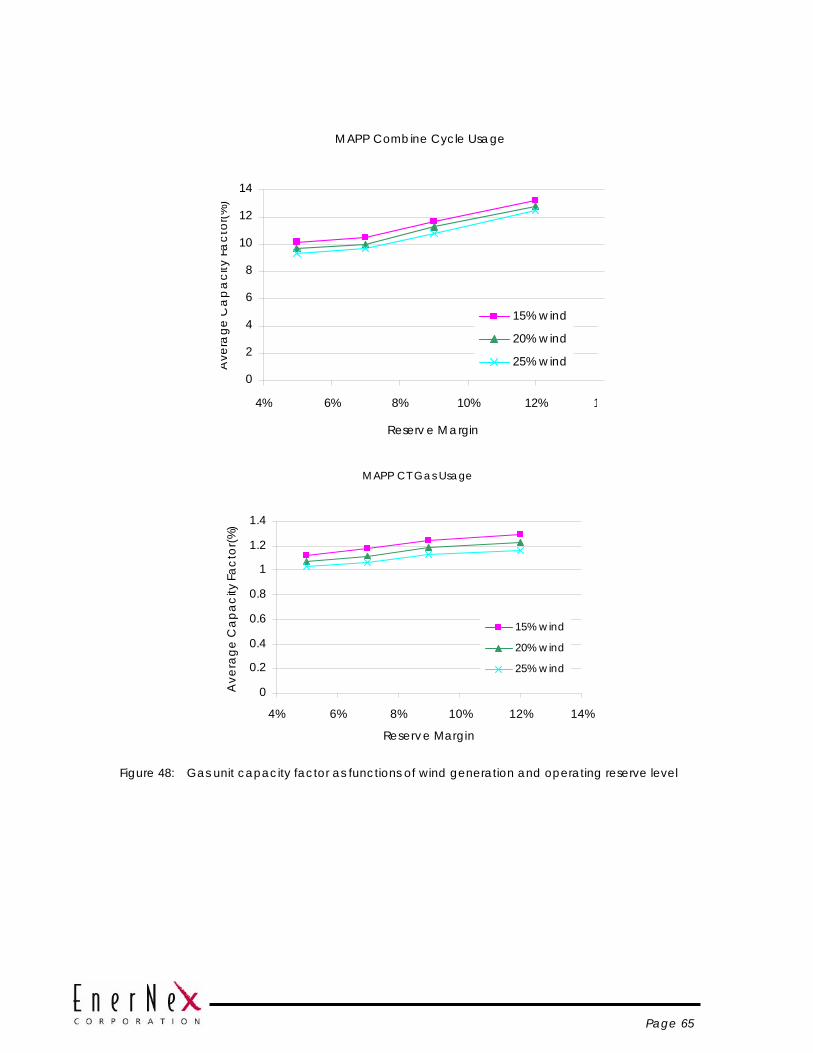
Page 65

MAPP Combine Cycle Usage

0

2

4

6

8

10

12

14

4% 6% 8% 10% 12% 1

Reserv e Margin

Ave

rage

Ca

pa

city

Fa

ctor

(%)

15% wind

20% wind

25% wind

MAPP CT Gas Usage

0

0.2

0.4

0.6

0.8

1

1.2

1.4

4% 6% 8% 10% 12% 14%

Reserve Margin

Ave

rage

Cap

acity

Fac

tor(%

)

15% wind

20% wind

25% wind

Figure 48: Gas unit capacity factor as functions of wind generation and operating reserve level

Page 66

MAPP Coal (<300MW) Usage

59

59.5

60

60.5

61

61.5

62

62.5

63

4% 6% 8% 10% 12% 14%

Reserv e Margin

Ave

rage

Ca

pa

city

Fa

ctor

(%) 15% wind

20% wind

25% wind

MAPP Coal(>=300MW) Usage

68.569

69.570

70.571

71.572

72.573

73.5

4% 6% 8% 10% 12% 14%

Reserv e Margin

Ave

rage

Ca

pa

city

Fa

ctor

(%)

15% wind

20% wind

25% wind

Figure 49: Coal unit capacity factor as functions of wind generation and operating reserve level

RESERVE COSTS The base cases investigated costs as a function of operating reserve level. In the market impact cases, a single operating reserve percentage for each level of wind generation was assumed, based on the analysis. The reserve level in the market impact cases was also perturbed by a small amount in additional cases. Finally, a case where the

Page 67

operating reserve level was varied according to the amount of wind generation actually being delivered each hour was run.

2004 load and wind generation patterns were used in this analysis.

Figure 50 summarizes all reserve cases run, showing production cost as a function of operating reserve level. A trend line based on an exponential fit has been added to each wind penetration level.

$1,880 M

$1,900 M

$1,920 M

$1,940 M

$1,960 M

$1,980 M

4.00% 6.00% 8.00% 10.00% 12.00% 14.00%

Total Operating Reserve

Prod

uctio

n C

ost 15% wind

20% wind

25% wind

Expon. (15% wind)

Expon. (20% wind)

Expon. (25% wind)

Figure 50: Production cost as a function of wind penetration and operating reserve level.

Production costs rise as total operating reserves are increased, which is the expected result. It is recognized, however, that a higher reserve requirement for all hours of the annual simulation is overly conservative, since there are many hours where wind generation is very low, and changes up or down would be of little note to operators. Further, an incremental operating reserve pegged to hourly changes in wind generation would not need to be comprised of spinning generation only – changes in the later part of the hour could be covered by quick-start units, if available. The significance here is that no costs accrue with this type of reserve unless it is used.

A case was run for the 2004 load patterns at 20% wind generation with operating reserves for wind generation modeled less conservatively:

• The additional operating reserve for wind generation is a variable hourly profile based on the previous hourly average value

• The incremental reserves for wind generation were further required only to be non-spinning.

As expected, these assumptions resulted in a decreased production costs over the fixed additional reserves case.

The cost associated with increased operating reserve can be placed in context by assigning it as an “integration cost” for wind generation and amortizing it over the wind energy delivered. Table 26 documents this calculation, and shows that for 20% wind generation, the fixed additional reserve options leads to a increased cost of $0.55 per

Page 68

MWH of wind generation over the case where no additional reserves are carried. If the additional reserve amount is varied according to the quantity of wind generation actually being delivered over the hour, the cost per MWH of wind energy falls to $0.23.

If the operating reserve margin intended to cover unexpected declines in wind generation in the next hour (i.e. the negative deviation from a persistence forecast) is all allowed to consist of non-spinning quick-start units, the reserve cost per unit of wind energy declines further, to just $0.11/MWH. An interpretation is that there is enough quick-start reserve available over most hours of the year. Reserve costs would only be incurred if generation needed to be committed to cover this reserve requirement.

In all of these cases, the reserve component of the integration costs seems modest. This is likely a consequence of the very large number and diversity of the controllable resources in the MN footprint, With more units in operation, an increase in the reserve requirement can be accommodate without significantly changing the commitment of units to operation.

Table 26: Incremental Reserve Cost for 20% Wind Case, 2004 Patterns

Case Production CostFull Reserves Case $1,928 M20% Variable Reserve Margin Case $1,923 MOperating Reserve Margin as non-spin $1,921 MBase Case - 5% Operating Reserve Assumption $1,919 M

Wind Production - 20%/2004 Cases 16,895,658 MWH

Inremental Cost - "Full" Reserves $9,368,744Cost per MWH Wind $0.55

Incremental Cost - "Variable" Reserves $3,955,303Cost per MWH Wind $0.23

Incremental Cost - Variable Reserves, non-spin $1,898,352Cost per MWH Wind $0.11

MARKET IMPACTS The market impacts cases assumed a single operating reserve level for each penetration of wind generation, per Table 18 . The operating reserve levels were 5.86% for 15% wind generation, 6.36% for 20% wind, and 7.05% for 25% wind.

The PROMOD results constitute an “optimized” market scenario since wind generation and load are known perfectly in both the commitment and dispatch steps. Actual market operation would not be as efficient, and therefore at least somewhat more costly. This will be investigated in detail in the unit commitment cost quantification.

A further point should be made regarding the relationship of PROMOD to the actual operation of the MISO energy markets. PROMOD searches for an optimal economic solution given load, unit cost characteristics and constraints, and system requirements. In real energy market operation, bidding strategies and the mechanics of the market may result in a somewhat different deployment of units. If the market is liquid and transparent, however, the behavior should track the results from a cost-based analysis.

The following charts and graphs illustrate the effect of wind generation on various metrics of the MISO market and aggregate impact on other generators in Minnesota.

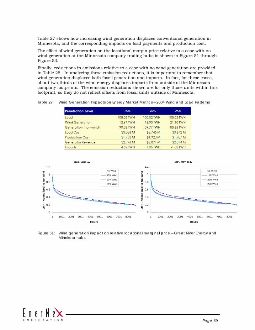
Page 69

Table 27 shows how increasing wind generation displaces conventional generation in Minnesota, and the corresponding impacts on load payments and production cost.

The effect of wind generation on the locational margin price relative to a case with no wind generation at the Minnesota company trading hubs is shown in Figure 51 through Figure 53.

Finally, reductions in emissions relative to a case with no wind generation are provided in Table 28. In analyzing these emission reductions, it is important to remember that wind generation displaces both fossil generation and imports. In fact, for these cases, about two-thirds of the wind energy displaces imports from outside of the Minnesota company footprints. The emission reductions shown are for only those units within this footprint, so they do not reflect offsets from fossil units outside of Minnesota.

Table 27: Wind Generation Impacts on Energy Market Metrics – 2004 Wind and Load Patterns

LMP - GRE Hub

0

0.2

0.4

0.6

0.8

1

1.2

1 1001 2001 3001 4001 5001 6001 7001 8001

Hours

LMP

- Nor

mal

ized

to N

o W

ind No Wind

15% Wind

20% Wind

25% Wind

LMP - MPC Hub

0

0.2

0.4

0.6

0.8

1

1.2

1 1001 2001 3001 4001 5001 6001 7001 8001

Hours

LMP

- Nor

mal

ized

to N

o W

ind No Wind

15% Wind

20% Wind

25% Wind

Figure 51: Wind generation impact on relative locational marginal price – Great River Energy and

Minnkota hubs

Page 70

LMP - MPL Hub

0

0.2

0.4

0.6

0.8

1

1.2

1 1001 2001 3001 4001 5001 6001 7001 8001

Hours

LMP

- Nor

mal

ized

to N

o W

ind No Wind

15% Wind

20% Wind

25% Wind

LMP - NSP Hub

0

0.2

0.4

0.6

0.8

1

1.2

1 1001 2001 3001 4001 5001 6001 7001 8001

Hours

LMP

- Nor

mal

ized

to N

o W

ind No Wind

15% Wind

20% Wind

25% Wind

Figure 52: Wind generation impact on relative locational marginal price – Minnesota Power and

Xcel Energy hubs

LMP - OTP Hub

0

0.2

0.4

0.6

0.8

1

1.2

1 1001 2001 3001 4001 5001 6001 7001 8001

Hours

LMP

- Nor

mal

ized

to N

o W

ind No Wind

15% Wind

20% Wind

25% Wind

LMP - SMP Hub

0

0.2

0.4

0.6

0.8

1

1.2

1 1001 2001 3001 4001 5001 6001 7001 8001

Hours

LMP

- Nor

mal

ized

to N

o W

ind No Wind

15% Wind

20% Wind

25% Wind

Figure 53: Wind generation impact on relative locational marginal price – Ottertail Power and

Southern Minnesota Municipal Power Agency hubs

Table 28: MN Company Emissions for ”No Wind” case and offsets for wind generation levels

No Wind( Metric Tons

x1000)15% (Base)

( Metric Tons x1000)20%

(Metric Tons x1000)25%

(Metric Tons x1000)

CO2 53670 -1839 -2627 -3500

SOx 106.1 -3.3 -4.9 -6.7

NOx 148.6 -6.3 -9.2 -12.4

Wind Generation Penetration

Page 71

THE COST OF INTEGRATING WIND GENERATION

Background The purpose of these hourly cases is to determine how the major characteristics of wind generation – variability and uncertainty – affect the commitment and dispatch of conventional generators.

The object of the analysis is to quantify the cost differential to serve the load not served by wind generation due to these characteristics. Using PROMOD and the data assembled for this study, this cost differential is determined through the following process:

1. Run PROMOD to simulate the MISO day-ahead market clearing and RAC (reliability assessment and commitment) process. In this step, the actual wind generation and load for the next day are not known perfectly. For wind generation, the day-ahead forecast developed in the resource characterization task is used. The load is more problematic. In the market clearing, demand bids, rather than actual forecasts, are used to clear the day-ahead offers. Later in the day, MISO performs a reliability assessment using security-constrained unit commitment, assesses this result versus the cleared offers. If the offers are short of what is determined necessary for reliability, more generation is committed. This process utilizes an actual forecast of load.

If load is assumed to be known perfectly, all uncertainty costs will be attributed to wind generation, which is not the case in reality. PROMOD performs the unit commitment part of the simulation using only “firm” demand and transactions. From this commitment, an economic dispatch is performed against both firm and non-firm load and transactions. So to represent the actual wind generation in this sub-step, a second wind energy transaction was created. This non-firm transaction consists of the difference between forecast and actual wind generation.

Load forecasts must also be handled through firm and non-firm transactions. In the commitment phase, firm transactions that represent the difference between actual and forecast loads are included. A non-firm transaction in the economic dispatch step is used to negate the firm transaction. What remains for dispatch, then, is the actual load.

2. A second reference case is analyzed with PROMOD where wind generation has no uncertainty or variability on a daily basis. The energy delivered over the course of each day, however, is identical to that in Step 1. Further, because of the attributes of this proxy energy resource, there are no additional reserves required to cover within the hour variability or short-term uncertainty.

3. The results of the unit commitment/economic dispatch simulation from the two cases are then compared. The differences in the load cost are assigned to the variability and uncertainty of wind generation.

The unit commitment component of the integration cost measures how the variability and uncertainty of wind generation decreases the efficiency of the market. The uncertainty impact shows up in the day-ahead market clearing, as significant wind generation forecast errors cause the market to respond to incorrect information. Over- and under-commitment of conventional generation will increase costs. The variability cost results from conventional units being dispatched “around” wind energy delivery. Increased costs result from less efficient operation of conventional units.

Page 72

Results of PROMOD Cases Case summary data and unit commitment cost calculations for the three wind generation penetration levels with 2003, 2004, and 2005 wind and load patterns are shown in Table 31. The numbers tabulated are for Minnesota loads and Minnesota companies. The total load shown is taken directly from the PROMOD output. This total includes retail load outside of Minnesota, and therefore is larger than the amount projected for the 2020 study year. As described in a previous section covering the development of the load model for the study, there is no practical way to segregate only the Minnesota load from the Minnesota company totals from the MISO West RSG PROMOD model.

These results show that, relative to the same amount of energy stripped of variability and uncertainty of the wind generation, there is a cost paid by the load that ranges from a low of $2.11 (for 15% wind generation, based on year 2005) to a high of $4.41 (for 25% wind generation, based on year 2003) per MWH of wind energy delivered to the Minnesota companies. This is a total cost and includes the cost of the additional reserves (per the assumptions) and costs related to the variability and day-ahead forecast error for wind generation. Integration cost results are shown graphically in Figure 54.

Unit Commitment Costs

$-

$1.00

$2.00

$3.00

$4.00

$5.00

15% Wind 20% Wind 25% Wind

Penetration Level

Inte

grat

ion

Cos

t ($

/MW

H W

ind

Ener

gy)

2003

2004

2005

Figure 54: Unit commitment costs for three penetration levels and pattern years. Cost of

incremental operating reserves is embedded.

IMPACTS OF WIND GENERATION ON UNIT UTILIZATION AND TRANSACTIONS Results from the PROMOD cases described thus far show that energy from wind generation displaces conventional generation in the Minnesota company footprint. Some of the displaced generation is from more expensive gas units, but with the resource profile and the relatively high penetration of wind generation in the lower load seasons, it is possible that baseload units could be impacted.

Page 73

An extra PROMOD case was run with the hourly dispatch profiles for all units in the Minnesota footprint larger than 200 MW reported. This case used 2004 load and wind patterns, and allowed PROMOD to optimize the solution (i.e. no wind generation or load forecast errors were considered). The analysis does appear to indicate some displacement of large coal generation by wind since production does go to zero for certain of the units throughout the year, not just during maintenance outage periods. Annual capacity factors however, remain 70% or greater for all of these units (not shown).

Wind generation also displaces imports into the Minnesota company footprint. Table 29 shows the load, wind generation, production from conventional generation, and imports for the 20% case with 2004 wind and load patterns. The table rows correspond to a case with no wind generation, and cases with different treatments of wind generation in the day-ahead unit commitment. If all wind generation is discounted in the day ahead commitment and allowed to show up in real time, about two-thirds of the wind generation would displace imports from outside of Minnesota. That amount is slightly increased if wind is incorporated, either through perfect knowledge or forecast, into the day-ahead commitment. This treatment increases production from Minnesota generators and further reduces imports.

Table 29: Load and Production for 20% Case, 2004 Patterns

CaseLoad (TWH)

Wind Generation

(TWH)Generation

(TWH)Import (TWH)

No wind 108.02 0.00 93.49 14.53 No Commit Credit 108.02 16.90 87.92 3.21

Forecast 108.02 16.88 89.72 1.42Perfect Forecast 108.02 16.90 89.77 1.35

EFFECT OF WIND GENERATION FORECASTING How wind generation is treated in the commitment process has influence on market operations. Table 30 provides financial numbers for the cases described in the previous section. In terms of straight production cost for the Minnesota companies, excluding wind generation from the day ahead commitment reduces production cost since the Minnesota generators are “backed down” by over 5 TWH from the “no wind” case, along with a reduction in imports. However, if the cost of imports is included in a modified “production cost” equation, the effect of forecasting can be seen.

The PROMOD case results did not include hourly imports and prices, so an estimate of the cost of the imports is necessary. The last column in Table 30 assumes an average price of $40/MWH for imports. The variable cost reduction – made up of production costs plus purchased energy – is about $19 million greater when wind generation forecasts are considered in the unit commitment over the case where wind generation shows up in real time. These reductions are summarized in Figure 55.

Of possibly more significance are the generation revenue and load payment reductions. Allowing wind to show up in real time introduces significant market inefficiencies that result in large reductions in both load payments and generator revenue. Although apparently a “good deal” for the loads, over the long term this would be detrimental for market function.

Wind generation forecasts are important to energy market efficiency. If the amount of wind generation considered in this study is excluded from the day-ahead market

Page 74

clearing and reliability assessment commitment, the market participants will effectively be responding to incorrect signals. Without considering the probable wind energy deliveries, generation will be offered into the market to serve load that does not appear.

Table 30: Summary of Case Results for various treatment of wind in unit commitment (2004 wind and load patterns)

CaseProduction Cost

($M)

Generation Revenue

($M)Load Cost

($M)Import (TWH)

Production Cost w/ Imports

($M)No wind 2041.16 3278.47 4136.42 14.53 2767.63

No Commit Credit 1875.33 2649.19 3488.41 3.21 2035.83Forecast 1928.06 2901.47 3756.69 1.42 1999.02

Perfect Forecast 1928.17 2891.47 3744.82 1.35 1995.78

0

500

1000

1500

2000

2500

3000

3500

Production Cost Reduction($M)

Generation RevenueReduction ($M)

Load Cost Reduction($M)

$ M

illion

Perfect ForecastNo Forecast Actual Forecast

Figure 55: Effect of wind generation forecast on Minnesota company production and load costs

Page 75

Table 31: Summary of Unit Commitment Cases: Variable Reserve, Load and Wind Forecast Error in Unit Commitment

15% Penetration/2003 Load Patterns 15% Penetration/2004 Load Patterns 15% Penetration/2005 Load Patterns

Block Mkt. Sim Delta Block Mkt. Sim Delta Block Mkt. Sim DeltaLoad 116.28 TWH 116.28 TWH Load 108.02 TWH 108.02 TWH Load 116.78 TWH 116.78 TWHWind Generation 12.56 TWH 12.56 TWH Wind Generation 12.66 TWH 12.66 TWH Wind Generation 12.83 TWH 12.83 TWHGeneration (non-wind) 92.87 TWH 94.94 TWH 2.06 TWH Generation (non-wind) 91.15 TWH 93.10 TWH 1.96 TWH Generation (non-wind) 92.94 TWH 94.98 TWH 2.03 TWHLoad Cost $4,423 M $4,460 M $37 M Load Cost $3,814 M $3,847 M $32 M Load Cost $4,430 M $4,457 M $27 MProduction Cost $2,017 M $2,069 M $52 M Production Cost $1,947 M $1,989 M $42 M Production Cost $2,016 M $1,952 M -$64 MGenerator Revenue $3,229 M $3,260 M $31 M Generator Revenue $2,972 M $2,982 M $10 M Generator Revenue $3,224 M $3,304 M $79 MWind Revenue $419 M $404 M -$16 M Wind Revenue $396 M $384 M -$13 M Wind Revenue $426 M $408 M -$19 MImports + Losses 10.84 TWH 8.78 TWH -2.06 TWH Imports + Losses 4.22 TWH 2.26 TWH -1.96 TWH Imports + Losses 11.01 TWH 8.98 TWH -2.03 TWHIntegration Cost - Unit Commitment (Load cost differential) $37 M Integration Cost - Unit Commitment (Load cost differentia $32 M Integration Cost - Unit Commitment (Load cost differential $27 MIntegration Cost $2.97 /MWH Integration Cost $2.55 /MWH Integration Cost $2.11 /MWH

20% Penetration/2003 Load Patterns 20% Penetration/2004 Load Patterns 20% Penetration/2005 Load Patterns

Block Mkt. Sim Delta Case Block Mkt. Sim Delta Block Mkt. Sim DeltaLoad 116.28 TWH 116.28 TWH Load 108.02 TWH 108.02 TWH Load 116.78 TWH 116.78 TWHWind Generation 16.75 TWH 16.75 TWH Wind Generation 16.88 TWH 16.88 TWH Wind Generation 17.16 TWH 17.16 TWHGeneration (non-wind) 92.02 TWH 95.06 TWH 3.03 TWH Generation (non-wind) 90.19 TWH 93.15 TWH 2.96 TWH Generation (non-wind) 92.04 TWH 95.09 TWH 3.05 TWHLoad Cost $4,313 M $4,382 M $68 M Load Cost $3,723 M $3,770 M $46 M Load Cost $4,317 M $4,364 M $46 MProduction Cost $1,990 M $2,059 M $69 M Production Cost $1,921 M $1,979 M $58 M Production Cost $1,988 M $2,009 M $22 MGenerator Revenue $3,136 M $3,260 M $124 M Generator Revenue $2,872 M $2,990 M $118 M Generator Revenue $3,123 M $3,237 M $114 MWind Revenue $540 M $518 M -$21 M Wind Revenue $513 M $493 M -$20 M Wind Revenue $550 M $524 M -$26 MImports + Losses 7.51 TWH 4.47 TWH -3.03 TWH Imports + Losses 0.96 TWH -2.01 TWH -2.96 TWH Imports + Losses 7.58 TWH 4.53 TWH -3.05 TWHIntegration Cost - Unit Commitment (Load cost differential) $68 M Integration Cost - Unit Commitment (Load cost differentia $46 M Integration Cost - Unit Commitment (Load cost differential $46 MIntegration Cost $4.09 /MWH Integration Cost $2.73 /MWH Integration Cost $2.71 /MWH

25% Penetration/2003 Load Patterns 25% Penetration/2004 Load Patterns 25% Penetration/2005 Load Patterns

Block Mkt. Sim Delta Block Mkt. Sim Delta Block Mkt. Sim DeltaLoad 116.28 TWH 116.28 TWH Load 108.02 TWH 108.02 TWH Load 116.78 TWH 116.78 TWHWind Generation 20.96 TWH 20.95 TWH Wind Generation 21.10 TWH 21.10 TWH Wind Generation 21.57 TWH 21.57 TWHGeneration (non-wind) 91.20 TWH 94.78 TWH 3.59 TWH Generation (non-wind) 89.22 TWH 92.77 TWH 3.55 TWH Generation (non-wind) 91.09 TWH 94.68 TWH 3.59 TWHLoad Cost $4,216 M $4,308 M $92 M Load Cost $3,644 M $3,704 M $60 M Load Cost $4,214 M $4,278 M $64 MProduction Cost $1,966 M $1,989 M $23 M Production Cost $1,894 M $1,967 M $73 M Production Cost $1,960 M $2,008 M $48 MGenerator Revenue $3,048 M $3,237 M $189 M Generator Revenue $2,801 M $2,974 M $173 M Generator Revenue $3,028 M $3,205 M $177 MWind Revenue $648 M $620 M -$29 M Wind Revenue $617 M $590 M -$27 M Wind Revenue $661 M $624 M -$37 MImports + Losses 4.13 TWH 0.54 TWH -3.59 TWH Imports + Losses -2.30 TWH -5.85 TWH -3.55 TWH Imports + Losses 4.12 TWH 0.53 TWH -3.59 TWHIntegration Cost - Unit Commitment (Load cost differential) $92 M Integration Cost - Unit Commitment (Load cost differentia $60 M Integration Cost - Unit Commitment (Load cost differential $64 MIntegration Cost $4.41 /MWH Integration Cost $2.83 /MWH Integration Cost $2.95 /MWH

Page 76

Section 6 CONCLUSIONS

The analytical results from this study show that the addition of wind generation to supply 20% of Minnesota retail electric energy sales can be reliably accommodated by the electric power system if sufficient transmission investments are made to support it.

The degree of the operational impacts was somewhat less than expected by those who have participated in integration studies over the past several years for utilities around the country. The technical and economic impacts calculated are in the range of those derived from other analyses for smaller penetrations of wind generation.

Discussion of the analytical results with the Technical Review Committee (TRC) and the Minnesota utility company representatives has established the following as the key findings and the principal reasons that wind generation impacts were not larger:

1. These results show that, relative to the same amount of energy stripped of variability and uncertainty of the wind generation, there is a cost paid by the load that ranges from a low of $2.11 (for 15% wind generation, based on year 2003) to a high of $4.41 (for 25% wind generation, based on year 2005) per MWH of wind energy delivered to the Minnesota companies. This is a total cost and includes the cost of the additional reserves (per the assumptions) and costs related to the variability and day-ahead forecast error for wind generation.

2. The cost of additional reserves above the assumed levels attributable to wind generation is included in the total integration cost. Special hourly cases were run to isolate this cost, and found it to be about $0.11/MWH of wind energy at 20% penetration by energy.

3. The TRC decision to combine the Minnesota balancing authorities into a single functional balancing authority had a significant impact on results. Sharing balancing authority functions substantially reduces requirements for certain ancillary services such as regulation and load following (with or without wind generation). The required amount of regulation capacity is reduced by almost 50%. Additional benefits are found with other services such as load following. In addition, there are a larger number of discrete units available to provide these services.

4. The expanse of the wind generation scenario, covering Minnesota and the eastern parts of North and South Dakota, provides for substantial “smoothing” of wind generation variations. This smoothing is especially evident at time scales within the hour, where the impacts on regulation and load following were almost negligible. Smoothing also occurs over multiple hour time frames, which reduces the burden on unit commitment and dispatch, assuming that transmission issues do not intervene to affect operations. Finally, the number of hours at either very

Page 77

high or very low production are reduced, allowing the aggregate wind generation to behave as a more stable supply of electric energy

5. The transmission expansion as described in the assumptions and detailed in Appendix A combined with the decision to inject wind generation at high voltage buses was adequate for transportation of wind energy in all of the scenarios. Under these assumptions, there were no significant congestion issues attributable to wind generation and no periods of negative Locational Marginal Price (LMP) observed in the hourly simulations.

6. The MISO energy market also played a large role in reducing wind generation integration costs. Since all generating resources over the market footprint are committed and dispatched in an optimal fashion, the size of the effective system into which the wind generation for the study is integrated grows to almost 1200 individual generating units. The aggregate flexibility of the units on line during any hour is adequate for compensating most of the changes in wind generation.

The magnitude of this impact can be gauged by comparing results from recent integration studies for smaller systems. In the 2004 study for Xcel Energy, for example, integration costs were determined to be no higher than $4.60/MWH for a wind generation penetration by capacity of 15%, which would be closer to 10% penetration on an energy basis.

7. The contribution of wind generation to power system reliability is subject to substantial inter-annual variability. Annual Effective Load Carrying Capability (ELCC) values for the three wind generation scenarios from rigorous Loss of Load Probability (LOLP) analysis ranged from a low of 5% of installed capacity to just over 20%. These results were consistent with those derived through approximate methods.

Page 78

Section 7 REFERENCES

[1] Xcel Energy and the Minnesota Department of Commerce: “Wind Integration Study – Final Report”, September, 2004; available at http://www.uwig.org/opimpactsdocs.html

[2] The New York State Energy Research and Development Authority (NYSERDA): “The Effects of Integrating Wind Power on Transmission System Planning, Reliability, and Operations”, March, 2005; available at http://www.uwig.org/opimpactsdocs.html

[3] Utility Wind Interest Group (UWIG): “Characterizing the Impacts of Significant Wind Generation Facilities on Bulk Power System Operations Planning” May, 2003 www.uwig.org

[4] Hirst, E. and Kirby, B. “Separating and Measuring the Regulation and Load Following Ancillary Services” November, 1998 (available at www.EHirst.com)

[5] Hirst, E. and Kirby, B. “What is the Correct Time-Averaging Period for the Regulation Ancillary Service?” April, 2000 (available at www.EHirst.com)

[6] Piwko, R., et.al. “The Effects of Integrating Wind Power on Transmission System Planning, Reliability, and Operations - Report on Phase 1: Preliminary Overall Reliability Assessment” for the New York State Energy Research and Development Authority (NYSERDA), published February, 2004 (available at www.nyserda.org/energyresources/wind.html)

[7] NREL/CP-500-26722: “Short-term Power fluctuation of Wind Turbines: Analyzing data from the German 250 MW Measurement Program from the Ancillary Services Viewpoint”

[8] Parsons, B.P, et. al. “Grid Impacts of Wind Power; A Summary of Recent Studies in the United States” presented at the 2003 European Wind Energy Conference, Madrid, Spain, June 2003.

[9] Milligan, M.R. “A Sliding Window Technique for Calculating System LOLP Contributions of Wind Power Plants” presented at the 2001 AWEA Windpower Conference, Washington, DC, June 4-7, 2001. NREL/CP-500-30363

[10] Milligan, M.R., et. al. “An Enumerative Technique for Modeling Wind Power Variations in Production Costing” presented at the International Conference on Probabilistic Methods Applied to Power Systems, Vancouver, BC, Canada, September 21-25, 1997. NREL/CP-440-22868

[11] Milligan, M.R., et. al. “An Enumerated Probabilistic Simulation Technique and Case Study: Integrating Wind Power into Utility Production Cost Models” presented at the IEEE Power Engineering Society Summer Meeting, Denver, CO, July 29 – August 1, 1996. NREL/TP-440-21530

Page 79

[12] Milligan, M.R., “Measuring Wind Plant Capacity Value” NREL White Paper

[13] Milligan, M. “Windpower and System Operation in the Hourly Time Domain” presented at the 2003 AWEA Windpower Conference, May 18-21, 2003, Austin, TX. NREL/CP-500-33955

[14] Hirst, Eric, “Interaction of Wind Farms with Bulk Power Operations and Markets” prepared for the Project for Sustainable FERC Energy Policy, September 2001

[15] Milligan, M.R. “A Chronological Reliability Model to Assess Operating Reserve Allocation to Wind Power Plants” presented at the 2001 European Wind Energy Conference, July 2-6, 2001, Copenhagen, Denmark. NREL/CP-500-30490

[16] Milligan, M.R. “A Chronological Reliability Model Incorporating Wind Forecasts to Assess Wind Plant Reserve Allocation” presented at 2002 AWEA Windpower Conference, June 3-5, 2002, Portland, OR. NREL/CP-500-32210

[17] Karady, George G., et. al., “Economic Impact Analysis of Load Forecasting”, IEEE Transactions on Power Systems, Volume 12, No. 3, August, 1997. pp. 1388 – 1392.

[18] L.L. Garver, Effective Load Carrying Capability of Generating Units IEEE Transactions on Power Apparatus and Systems VOL PAS-85, No 8, pp 910-919 August, 1966

Page 80

APPENDIX A – WEST RSG STUDY ASSUMPTIONS

Note: The following is a reproduction of the assumptions document for the West Regional Studies Group (RSG) dated May, 2006. The base model for the West RSG is the starting point for the Minnesota PUC wind integration study.

INTRODUCTION There are several exploratory studies performed in West Region. These studies are: CapX 2020, Buffalo Ridge Incremental Generation Outlet (BRIGO) study, Southwest Minnesota to Twin Cities EHV Development study, Southeastern Minnesota – Southwestern Wisconsin Reliability Enhancement Study, American Transmission Company (ATC) Access Project study, NW Exploratory study, Iowa-Southern Minnesota exploratory study. The transmission upgrades proposed in these studies are corresponding to their generation scenario assumptions.

The West RSG is a collaborative effort of MISO staff, the MISO Transmission Owners, stakeholders, regulatory staff and a voluntary participation of SEAMS transmission owners to direct the studies for the MISO Transmission Expansion Plan. Midwest ISO is trying to roll the results of all the above exploratory studies into one study – West RSG Exploratory Study. This collaborative study will be included in MTEP for information purpose. The Goal of this collaborative study is to determine if transmission needs to be built for energy delivery, REO or economics. It can also determine multi-use requirements that may not be supportable by a single entity.

The West RSG study is based on the MAPPMAIN reduced footprint, the topology is shown in the above figure, a total of 34 companies are included in the MAPPMAIN reduced footprint.

FUEL FORECAST3 The source for the fuel forecasts in the Powerbase database is the Platt’s database, Henry hub forecasts and EIA forecasts. New Energy Associates (NEA) contracts with Platt’s for various fuel forecasts. NEA starts with Platt’s forecasts for natural gas and then uses the basis differential inherent in Platt’s forecast for Natural Gas combined with NYMEX Henry Hub futures prices for the first 18 months of the forecast. For the forecast beyond 18 months, the Energy Information Administration (EIA) natural gas forecast for the Henry Hub serves as the base index. The basis differential to each area are then applied against the EIA forecast of the Henry Hub prices.

West RSG study will be a multi-year study. The base case is set at year 2020. Starting from the 2011 fuel forecast in the Powerbase, we scaled the gas price within MAPPMAIN footprint to $9.00/mmBtu. As we added new coal plants into the CAPX study the coal price used is $1.77/mmBtu. All the new coal plants should run at a 60% and above

3 Platts Fuel Forecasting methodology, found on NEA PowerBase support web site

Page 81

capacity factor range. Based on this assumption, the Boswell Energy Center Coal price is set as $1.77/mmBtu and all other coal prices are adjusted accordingly.

LOAD FORECAST The CAPX companies provided the 2020 load forecast for the following control areas: ALTW, NSP, MP, SMMP, GRE, OTP and DPC. In PROMOD, there are two companies within the OTP control area: Otter Tail Power Co. and Minnkota Power Coop. The load forecast for OTP control area is then distributed to two companies respectively. The detailed load forecast for all CAPX companies are listed in Table 32. Other companies’ load forecast stay as 2011 load forecast from Powerbase.

Table 32

Peak Load at 2020 (MW)

Annual Energy in 2020 (GWH)

GRE 3894 19677.3 ALWST 3888.2 19728.2 DPC 1266.2 6675.0 MPL 1814.4 12674.0 NSP 12885.1 67017.6 SMMP 442.4 2512.8 MPC 1080.8 7048.4 OTP 1167.5 6844.0 Total 26438.6 142177.3

GENERATING UNITS AND PARAMETERS

Existing Units Typically as a part of PROMOD model development process, MISO verifies generators in the default Powerbase database against the MISO loadflow models. Stakeholders are involved in this process: Expansion Planning Working Group (reporting to Planning Sub-Committee) is sent a list of generators mapped to load flow models and member comments are solicited. Different Regional Study Groups (RSG) are also involved at times. MISO has 3 RSG’s: Central, East and West modeled according to the Operation regions. For the CAPX study the West RSG helped verify generators in the CAPX study area.

New units for West RSG study To serve the increased load in West RSG area (around 6000MW load increase), Generation Interconnection requests submitted in MISO queue are recommended as a generation scenario. These requests are distributed in West region (except Wisconsin), and the total capacity is 6689 MW, in which 2948 MW is renewable resource. All new generators are created from the similar existing generators in Powerbase, with the fuel set as $1.77/mmBtu for coal generators and $9.00/mmBtu for Gas turbine. The detailed list of new generators can be found in Appendix B.

Page 82

TRANSMISSION UPGRADES West RSG study is based on MTEP06 Phase 2 power flow model. In corresponding to the new generation/load increase, the following transmission upgrades are added, which are based on the recommended facilities from several studies in West region.

o Big Stone II interconnection/delivery upgrades (Alternative 1)

o Common facility upgrades recommended both in Minnesota and North/West bias scenarios in CapX 2020, Boswell-Wilton 230kV line is also included;

o Facility upgrades recommended in Buffalo Ridge Incremental Generation Outlet (BRIGO) study;

o Facility upgrades recommended in Southwest Minnesota to Twin Cities EHV Development study;

o Facility upgrades recommended in Southeastern Minnesota – Southwestern Wisconsin Reliability Enhancement Study;

o Some facility upgrades recommended in ATC Access project study, including Paddock-Rockdale project (P-R), LaCrosse-Columbia project (portion of Prairie Island-Columbia), and Salem-North Madison (S-NM) project.

o Some facility upgrades recommended in Iowa-Southern Minnesota exploratory study, including Hazelton-Salem, Salem-Nelson Dewey-Spring Green 345 kV lines.

The line list for these projects can be found in Table 33.

Page 83

Table 33: New Transmission Lines in West RSG Study

From To kV Miles Comments Alexandria Monticello 345 CapX Alexandria Maple River 345 126 CapX Antelope Valley Maple River 345 292 CapX Arrowhead Chisago 345 120 CapX Arrowhead Forbes 345 60 CapX Benton County Chisago County 345 59 CapX Benton County Granite Falls 345 110 CapX Benton County St. Boni 345 62 CapX Blue Lake Ellendale 345 200 CapX Chisago County Prairie Island 345 82 CapX Columbia N. LaCrosse 345 80 CapX, ATC Ellendale Hettinger 345 231 CapX Rochester N. LaCrosse 345 60 CapX, ATC, SE_MN-SW_WI, ISMN Prairie Island Rochester 345 58 CapX, ATC, SE_MN-SW_WI, ISMN Boswell Wilton 230 CapX Big Stone Ortonville 230 BS II Ortonville Johnson Jct. 230 BS II Johnson Jct. Morris 230 BS II Big Stone Canby 230 BS II Canby Granite Falls 230 BS II Alexandria 345/115 CapX Alex Sauk Ct 115 25 CapX Sauk Ct Melrose 115 10 CapX Melrose Albany 115 15 CapX Albany W. St. Cloud 115 25 CapX Lk Yankton Marshall 115 BRIGO Nobles Fenton 115 BRIGO Nobles Nobles 345/115 BRIGO Marshall SW Sub MRES Brookings Co Lyon Co 345 CAPX (SW_MN-TC) Lyon Co Franklin 345 double CAPX (SW_MN-TC) Franklin Helena 345 double CAPX (SW_MN-TC) Helena Lk Marion 345 CAPX (SW_MN-TC) Lk Marion Hampton Corner 345 CAPX (SW_MN-TC) Lyon Co Hazel 345 CAPX (SW_MN-TC) Brookings Co Yankee 115 CAPX (SW_MN-TC) Brookings Co Toronto 115 CAPX (SW_MN-TC) Hazelton Salem 345 70 ISMN Salem N Madison 345 ATC, ISMN Paddock Rockdale 345 ATC Lakefield Winnebago 345 ISMN Winnebago Hayward 345 ISMN Hayward Adams 345 ISMN

Page 84

APPENDIX B - WEST RSG STUDY NEW GENERATING UNITS

MISO Project Num

Bus numb Bus name Pmax Pmin Qmax Qmin

MISO Queue Date

Control Area County State

In Service Date Study Status

IA Status Project manager

Interconnection Service Type Fuel Type

NE group

G424 61710 MINNTAC7 100 0 0.00 0.00 19-Apr-04 MN St. Louis MN 01-Dec-06 FEC SIC FE Diwakar Tewari ER Wind

G509 61705 BABBITT7 75 0 0.00 0.00 18-Mar-05 MP St. Louis MN 01-Aug-06 FEC SIE Diwakar Tewari NR Wind

G519 61625 BLCKBRY4 580 0 190.64 -190.64 19-May-05 MP Itasca MN 01-Apr-09 SIE Diwakar Tewari NR

Coal and/or a blend of Petroleum coke and coal

G591_592 60101 FORBES 2 800 0 262.95 -262.95 25-Jan-06 MP St. Louis MN 01-Mar-13 FEP Raja Srivastava NR Coal

G597 61625 BLCKBRY4 606 0 199.18 -199.18 14-Feb-06 MP Itasca MN 01-Jan-13 FEP Ron Arness NR Coal

G600 63254 VIKING 7 110 0 0.00 0.00 16-Feb-06 OTP Marshall MN 31-Dec-08 FEP Ron Arness ER Wind

ND group

G380 63279 RUGBOTP7 150 0 0.00 0.00 21-Nov-03 OTP Pierce ND 01-Dec-05 IC/FC IAF Kun Zhu ER Wind

G531 63049 STANTON4 80 0 26.29 -26.29 01-Jul-05 GRE Mercer ND 01-Apr-09 SIE Raja Srivastava NR Coal

G581 66791 CENTER 3 600 0 197.21 -197.21 27-Dec-05 MP Oliver ND 01-Jan-15 FEP Raja Srivastava NR Coal

G607 67316 COYOTE 3 25 0 8.22 -8.22 01-Mar-06 OTP Mercer ND 25-Oct-08 FEP Ron Arness NR Coal

Group 4

G389 63043 ELK RIV4 200 0 65.74 -65.74 03-Nov-03 GRE Sherburne MN 01-Jan-07 IP Raja Srivastava NR Natural Gas

G390 63043 ELK RIV4 100 0 32.87 -32.87 03-Nov-03 GRE Sherburne MN 01-Jan-09 IP Raja Srivastava NR Natural Gas

G417 60896 SHAKOPE8 15 0 4.93 -4.93 22-Mar-04 NSP Scott MN 31-Dec-05 IP Raja Srivastava NR biomass

G474 63220 ELBOWLK7 20 0 0.00 0.00 01-Oct-04 OTP Grant MN 01-Nov-05 IP Raja Srivastava NR Wind

G489 60119 LKYNKTN7 20 0 0.00 0.00 19-Jan-05 NSP Lyon MN 01-Oct-06 IP Raja Srivastava NR Wind

G491 60715 CHANRMB9 150 0 0.00 0.00 29-Dec-04 NSP Pipestone MN 01-May-07 FEP Raja Srivastava NR Wind

G502 66752 DRAYTON4 50 0 0.00 0.00 14-Mar-05 MP Oliver ND 01-Nov-05 SIC FE Raja Srivastava NR Wind

G514 60331 LKFLDXL3 200 0 0.00 0.00 20-Apr-05 NSP Jackson MN 01-Oct-06 FEE Raja Srivastava NR Wind

G517 34226 STORDEN8 150 0 0.00 0.00 02-May-05 ALTW Cottonwood MN 01-Oct-06 SIE Raja Srivastava NR Wind

G518 62371 WLKFLTP 8 0 0.00 0.00 02-May-05 GRE Jackson MN 01-Nov-06 FE Raja Srivastava NR Wind

Page 85

MISO Project Num

Bus numb Bus name Pmax Pmin Qmax Qmin

MISO Queue Date

Control Area County State

In Service Date Study Status

IA Status Project manager

Interconnection Service Type Fuel Type

G520 60119 LKYNKTN7 150 0 0.00 0.00 20-May-05 NSP Lyon MN 31-Dec-06 SIE Raja Srivastava NR Wind

G530 34164 GR JCT 9 14 0 0.00 0.00 15-Jun-05 ALTW Greene IA 01-Sep-06 IP Raja Srivastava NR Wind

G532 62792 ODIN 19.95 0 0.00 0.00 06-Jul-05 ALTW Cottonwood/Watonwan MN 01-Sep-06 IP Raja Srivastava NR Wind

G536 62371 WLKFLTP 20 0 0.00 0.00 20-Jul-05 ALTW Jackson MN 01-Oct-06 SIE Raja Srivastava NR Wind

G538 34137 TRIBOJI5 150 0 0.00 0.00 08-Aug-05 ALTW Dickinson IA 01-Oct-06 FEP Raja Srivastava NR Wind

Group 5

G540 34015 LIME CK5 80 0 0.00 0.00 01-Sep-05 ALTW Worth IA 31-Dec-07 NR Wind

G548 34015 LIME CK6 80 0 0.00 0.00 17-Sep-05 ALTW Worth IA 31-Dec-06 NR Wind

G551 34371 RICE 8 100 0 0.00 0.00 27-Sep-05 ALTW Howard IA 01-Sep-07 NR Wind

G552 62053 MAPLE H8 50.4 0 0.00 0.00 28-Sep-05 ALTW Emmet IA 01-Aug-06 NR Wind

G555 66555 MORRIS 7 100 0 0.00 0.00 24-Oct-05 OTP Stevens MN 01-Nov-07 NR Wind

G573 64239 FRANKLN5 80 0 0.00 0.00 09-Dec-05 ALTW Franklin IA 01-Oct-06 NR Wind

G574 64239 FRANKLN6 80 0 0.00 0.00 09-Dec-05 ALTW Franklin IA 30-Sep-07 NR Wind

G575 64239 FRANKLN7 40 0 0.00 0.00 09-Dec-05 ALTW Franklin IA 01-Oct-06 NR Wind

G576 60128 SPLT RK5 40 0 0.00 0.00 12-Dec-05 GRE Rock MN 01-Sep-07 ER Wind

G586 60050 YANKEE 1 30 0 0.00 0.00 30-Dec-05 NSP Lincoln MN 01-Jun-07 NR Wind

G587 60728 FRANKLN8 20 0 0.00 0.00 30-Dec-05 NSP Sibley MN 01-Jun-07 NR Wind

G589 34018 HAZLTON3 750 0 246.51 -246.51 12-Jan-06 ALTW Black Hawk IA 01-Dec-09 NR Coal

G593 34007 LAKEFLD5 100 0 0.00 0.00 07-Feb-06 ALTW Jackson MN 01-Oct-07 NR Wind

G594 62369 ROUND LK 50 0 0.00 0.00 07-Feb-06 GRE Jackson MN 01-Oct-07 NR Wind

G595 34139 HANCOCK5 210 0 0.00 0.00 13-Feb-06 ALTW Hancock IA 30-Jul-07 ER Wind

G602 60369 FENTON 31.5 0 0.00 0.00 23-Feb-06 NSP Nobles MN 01-Nov-07 NR Wind

G604 62886 OWATONNA 47.5 0 0.00 0.00 27-Feb-06 Steele MN 01-Nov-06 ER Wind

G608 60760 PAYNES8 6.3 0 0.00 0.00 02-Mar-06 Pope MN 01-Oct-06 ER Wind

G612 34071 FERNALD7 150 0 0.00 0.00 20-Mar-06 ALTW Story IA 31-Aug-07 ER Wind

G614 34008 FOX LK5 250 0 0.00 0.00 24-Mar-06 NSP Emmet/Dickinson IA 01-Jul-07 NR Wind

Exira #3 67469 EXIRA 3G 40 0 MRES 1-Jun-07 Gas

Page 86

APPENDIX C – METHOD FOR CONVERTING WIND

SPEED DATA TO WIND GENERATION

Meteorological simulations for creating chronological wind speed data has greatly enhanced the value of wind integration studies. It is not possible to generate a separate wind speed profile for each turbine in the wind generation scenario. Each profile, therefore, must represent a number of turbines located in the general vicinity of the model extraction point.

The objective of this exercise is to determine a method for calculating hourly wind generation from the measured wind data. The turbine power curve from Figure 56 is used.

Figure 56: Turbine power curve used for calculating generation data from wind speed

measurements.

Measurement data from an operating wind plant with 30 of the turbines referenced above, consisting of wind speed and plant power at ten minute intervals was processed to create a “plant” power curve. This curve is shown in Figure 57.

Page 87

Figure 57: Empirical “Power Curve” for wind plant from measured values.

Figure 58 shows the results of applying the power curve from Figure 56 (scaled appropriately) to 10-minute wind speed data, then aggregating the results to hourly average values. The striking feature of this figure is the “fuzziness.” If the wind speed data were averaged to hourly values before applying the power curve, the characteristic would match that shown in Figure 56: Turbine power curve used for calculating generation data from wind speed measurements.. The difference, of course, is that the mathematical operations are not the same because of the nonlinear nature of the turbine power curve.

Figure 58: Wind plant “power curve” calculated from 10-minute wind speed values.

A closer comparison (Figure 59) of the calculated and measured wind generation reveals that the simple transformation from wind speed to power using a single power curve and wind speed value leads to a calculated value that is higher than the actual, and a

Page 88

tendency to “saturate” during periods of high wind, sometimes unlike the measured data. A computation of the energy delivered shows that the calculated value is about 25% higher than what was actually metered.

Figure 60 illustrates this qualitatively. The “knee” of the calculated plant power curve is much more pronounced, although the “fit” is reasonable at lower power levels. Therefore, shifting the plant power curve to the right to approximately account for the diversity of wind speeds over the plant area would degrade the fit at lower wind speed levels.

Figure 59: Calculated vs. Measured wind generation.

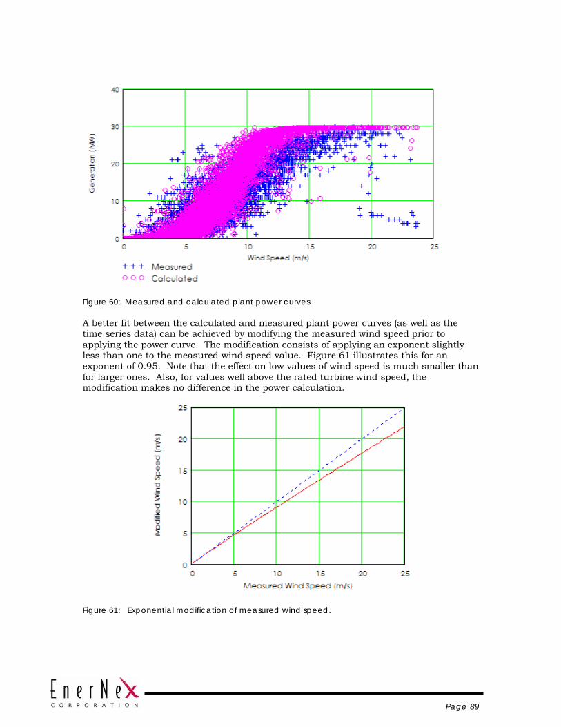
Page 89

Figure 60: Measured and calculated plant power curves.

A better fit between the calculated and measured plant power curves (as well as the time series data) can be achieved by modifying the measured wind speed prior to applying the power curve. The modification consists of applying an exponent slightly less than one to the measured wind speed value. Figure 61 illustrates this for an exponent of 0.95. Note that the effect on low values of wind speed is much smaller than for larger ones. Also, for values well above the rated turbine wind speed, the modification makes no difference in the power calculation.

Figure 61: Exponential modification of measured wind speed.

Page 90

The comparison of measured and actual power curves using this modification is shown in Figure 62. The calculated energy over the entire year for the calculated data differs by less than 1% from the measured data.

Figure 62: Measured and modified calculated plant power curves.

The improvement is also evident in the time series data. Figure 63 shows the same time periods from Figure 59, with the calculated value here based on a modified wind speed value. The improvement over the very simplified method using just the single turbine power curve is evident.

Page 91

Figure 63: Comparison of measured wind generation to that calculated with wind speed

modification.

=