Embed Size (px)
Citation preview

42 Middle East Well Evaluation Review
Analysis of waves passing through rocks
is taking a new direction. Geophysicists,
keen to maximize the benefits from
seismic data, are gleaning fresh
information about formations by
analysing some of the more unusual
waveforms contained in their data.
They are also using advanced
reprocessing techniques to clarify the
seismic picture. Carl Poster, Andy Fryer
and Iain Buchan outline some of the new
approaches.
Analysis of old seismic data, gathered
almost a decade ago, is also helping the
search for water in the region. Don
Hadley, Christopher Menges and Dennis
Woodward of the United States Geological
Survey explain how seismic data can be
used to help locate groundwater
resources.

43Number 10, 1991.
Photo: Wave rock, Hyden, Western Australia (Tony Stone)

44 Middle East Well Evaluation Review
Mixing oil and water
Seismic data amassed for oil explo-
ration is now being reprocessed in
the United Arab Emirates and is
revealing new knowledge on water
resources. This reprocessing work,
believed to be the first of its kind, is part
of a water resources project covering
hundreds of square kilometres of desert
bordering the western margins of the
Oman mountains. The investigation is
being undertaken by the United States
Geological Survey (USGS) and the
UAE’s National Drilling Company (NDC),
with technical support from the Abu
Dhabi National Oil Company (ADNOC).
Altogether, a team of about 50 people is
working on the project.
Abu Dhabi is keen to find new sup-
plies of water. A rapid growth in popula-
tion, plus increased reclamation of land
for agriculture, has stimulated demand
for freshwater from 54 to 89 million gal-
lons per day in the last 10 years. Over
the last 20 years, demand has risen 10-
fold.
Much of the annual runoff from the
Oman mountains enters the alluvial fill
lying beneath the desert’s dunes.
Geological field studies, and examina-
tion of existing water wells, indicates
there are two formations that can serve
as aquifers for this water - a coarse grav-
el of Quaternary age and, beneath, a
slightly older and finer-grained mixture
of gravel and mudstone. With larger
pores, less silt and higher permeability,
the upper aquifer is the better of the
two.
There were two main problems con-
fronting the hydrogeologist studying
T h e G u l f
0 50 100 km Saudi Arabia
Liwa Area
Al Ain Area
Abu Dhabi
Dubai
Oman
Jebel Hafit
Om
an O
man M
ountains
Buraimi Al
Jaww Plain
Gulf of
Oman
Fig. 4.1: National Drilling Company rig ND-85 at NDC/USGS well no. GWP-30. The well is
located about 20km north of Al Ain and 2.5km west of the Al Ain - Dubai Highway. The
well is being logged and sidewall cored by a Schlumberger logging unit from Abu
Dhabi.(Photo courtesy USGS/NDC).
Fig. 4.2: Abu
Dhabi has two
main sources
of
groundwater -
to the west of
the Oman
mountains
around Al Ain
and in the
more southerly
Liwa region.
these zones: what is the regional level of
the water table, and where are the best
places to drill the aquifers? Numerous
tools are available to the hydrogeologist:
* Satellite imagery shows the regional
surface geology in great detail,
* Field studies of outcrops indicate
the character of the aquifers in some
areas,
* Logging of test wells and monitoring
of existing wells provides some informa-
tion on the aquifers’ thickness, proper-
ties and extent.
However, the groundwater explo-
rationists in the UAE needed a detailed
view of the aquifers’ subsurface proper-
ties over a very large area. They decided
to look at ADNOC’s maps, showing seis-
mic coverage for past oil exploration.
The region had been densely covered
with seismic lines and numerous shal-
low velocity measurements had been
made in boreholes. The seismic data,
they hoped, would show evidence of
shallow structures affecting the aquifers,
and the shallow velocity results might
give an indication of the regional stratig-
raphy, and thus the freshwater-bearing
rocks.
However, the seismic data had been
originally processed to show deeper
images of interest to the oil explo-
rationists. To get an improved view of
events nearer the surface, the data had

45Number 10, 1991.
Fig. 4.3: The photograph at the top shows the surface terrain of the aquifer near Al Ain. Most of the recharge is in the form of
runoff from the mountains in the background. The tracks of the vibrators which were used by surface seismic crews can be seen
in the foreground. The seismic data at the bottom of the illustration revealed the area’s subsurface structure and stratigraphy. It
was essential to find the deeper, thicker parts of the aquifers so that the wells could be correctly positioned.
A geological model was constructed (centre) from geological, well and seismic data. The character and thickness of each
formation was determined in detail from the logs. Their lateral extent and regional structure was provided by the surface seismic
data. A synthetic seismogram was computed from sonic and density logs (inset) and this confirmed that there was a good match
between the log and seismic data.

46 Middle East Well Evaluation Review
to be re-processed using a slightly dif-
ferent approach. The first step was to
remove the lower frequencies (below
about 20Hz) from the original data, and
it was observed that shallower events
were enhanced. For normal, deeper tar-
gets, the higher frequencies are attenu-
ated, and it is necessary to keep the
lower frequencies in the data.
Next, the statics were recomputed to
a datum level nearer the surface
(Middle East Well Evaluation Review,Number 8, 1990). The purpose was to
exclude from this correction large thick-
nesses of deeper material for which
there are no direct measurements of
velocity. This reprocessing step signifi-
cantly enhanced the section.
Then the stacking operation was
repeated. The velocities were deter-
mined from the pre-stack data at a con-
siderably closer spacing than originally
used. Also, test stacks were produced to
determine which trace offsets improved
and which degraded the stack at shal-
low depths. Only those traces which
gave a clear image were used in the
final stacking process.
Finally, and perhaps the most impor-
tant factor in the re-processing, was the
close co-ordination between the pro-
cessing group at GECO and the hydro-
geologists. The data processors had to
clearly understand the objectives and
targets of the interpreters, and made
repeated tests and preliminary versions
before a final section was selected.
To solve the problem of mapping the
water’s surface, the hydrogeologists
turned to the shallow wells used to
measure velocities near the surface. It
was these holes that were used to deter-
mine the static corrections used in the
reprocessing. As water saturation in the
alluvial fill significantly increases seis-
mic velocities, they were able to anal-
yse the arrival times of the seismic sig-
nal versus depth and locate the point in
each well at which the velocities sud-
denly increased. A map of these depth
points provided an accurate view of the
water table’s surface.
Multiple vision
One of the oldest problems plaguing
seismic interpreters is how to confident-
ly identify real events on a seismic sec-
tion. Is the event seen by the interpreter
a true reflection, perhaps from a poten-
tial reservoir, or is it a multiple, ringing
down from the near-surface? Figure 4.6
shows one onshore example in the
southern Gulf. The section, part of a 3-D
data set, shows prominent, flat events
Fig. 4.4: Demand
for water in Abu
Dhabi has
increased 10-fold
in the past two
decades.
220
210
210
230
230
220
200
230
240
250
240
240
250
250
260
260
270
280
280
280 29
0
290
Buraimi
Al Ain
340
320
310
300
310
290
300
320 33
0 34
0
350
360
370 39
0
0 50km
200
190
Bou
ndar
y of
con
cess
ion
area
N
Application of uphole data from petroleum seismic surveys to
groundwater investigations, Abu Dhabi (United Arab
Emirates), by D. Woodward and C. Menges. Published in
Geoexploration, 28 (1991). Elsevier Science Publishers B.V.,
The Netherlands.
Fig. 4.5: Altitude of water near Al
Ain, calculated from uphole
data, 1981-83. The higher
altitudes run parallel to the
mountains to the east and the
contours drop smoothly towards
the west.
47Number 10, 1991.
crossing the shallow portion
(around 400ms), which possibly
contained a reservoir. However,
multiples were thought to be
strongly generated in this area
and, even though the section had
been processed to try to remove
them, the interpretation prior to
the drilling was suspect.
However, before the start of
the oil well, a water well had been
drilled at the site to provide water for
the subsequent drilling programme. It
was realized that the well, about 600m
deep, could accommodate a VSP, which
should be able to provide considerable
assistance in discriminating true from
false reflections both above and below
the well’s TD.
To produce a data set, a VSP was
acquired over 30 levels with a 20m inter-
val. Also, a full suite of logs was
obtained to provide geological control
for the VSP’s interpretation. The VSP
was processed in the usual manner and
close attention was paid to the downgo-
ing waves which should contain consid-
erable information on the multiple pat-
tern. By analysing that part of the VSP, a
very good idea of the extent of multi-
ples in the final upgoing wavefield could
be established. A comparison of this
with the seismic section would indicate
the degree to which multiples were pre-
sent.
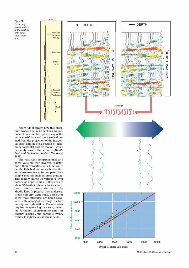
A simple way to indicate the extent
of multiples on the downgoing VSP
waves is to compute its autocorrelation
function. This function is simply the
result of shifting the trace in steps rela-
tive to itself, multiplying the two togeth-
er, and plotting the product against the
total shift. When the original trace
repeats itself, the autocorrelation func-
tion is high at that point.
Figure 4.7 shows the initial downgo-
ing trace and its autocorrelation func-
tion; note the ‘ringiness’ in both. After
the application of predictive, or
‘gapped’ deconvolution (the parameters
of which are selected on the basis of the
autocorrelation results) the downgoing
wavetrain and its autocorrelation func-
tion have been significantly smoothed.
This same processing is applied to
the VSPs upgoing waves, which are
stacked into a final single trace. Figure
4.7 shows this stack, played out four
times. (In addition to the processing
noted previously, an additional wavelet
deconvolution operation has been
applied, to compress the wavelet visible
in figure 4.7 to a short, zero-phase
pulse.) In the figure, the VSP is juxta-
posed with the geological details, indi-
cated by the interpreted well logs scaled
into time.
Based on the analysis of the downgo-
ing wave field, the final VSP stack in fig-
After predictive deconvolution
Fig. 4.7: (Top): Both the VSP downgoing waves
and their autocorrelation functions (right)
have a high degree of ‘ringiness’ before
predictive deconvolution. After processing
(below) both sets of traces have been
smoothed significantly.
Fig. 4.6: Seismic
section from the
southern Gulf. How
do you differentiate
the real events
from the multiples?
Computing the
autocorrelation
function may help.
100ms100ms
Before predictive deconvolution

48 Middle East Well Evaluation Review
ure 4.7 is assumed to be multiple-free.
By comparing this with the seismic sec-
tion in figure 4.7 a very good correlation
of events can be seen, and indicates
that the events in question are real
reflections.
Using the water well for VSP acquisi-
tion before the main drilling program,
provided valuable information for inter-
preting this section and proved to be a
cost-effective method for obtaining seis-
mic processing parameters. A VSP in
the oil well, obtained over a much deep-
er section, of course extended this infor-
mation.
Fig. 4.8:
EVENTFUL
PROCESSING:
There is now a
good correlation
between the
upgoing VSP stack
(right), the surface
seismic (centre)
and log data. The
seismic signature
of the shallow
aquifer (ringed)
can be determined
by correlating the
interpreted open-
hole logs with the
VSP (far right
traces) and then
the surface
seismics (centre).
Since the VSP has
both a time and
depth scale, the tie
of the interpreted
logs and the events
on the VSPs is
unambiguous.
As the VSP has
been determined to
be free of
multiples, the good
correlation with
the surface
seismics indicates
that it too is mainly
multiple free.
Sensor achievement
Solving these problems with seis-
mic methods rests on one key
requirement - good data. Good
seismic data for the geophysicist
has several qualifications. It
should first of all have a high sig-
nal-to-noise ratio, with minimum
noise originating from the sensor
system itself. Then, it should have
a wide bandwidth, and include as many
frequencies as possible while maintain-
ing the signal’s original phase.
Next, it is important that the orienta-
tion of the sensor has a minimum effect
on the signal, especially in the bore-
hole. Seismic waves come from all
directions, and if the same sensor can
be positioned in vertical and horizontal
orientations without introducing its own
distortions, the three-dimensional
results from the data will be more reli-
able.
Finally, the data should have a large
dynamic range, so that the interpreter
can see and accurately compare low
and high amplitude reflections.
A new seismometer which fills many
of these requirements is now becoming
available for borehole seismic acquisi-
tion. Conventional sensors’ signals
come from motion above their natural
frequency, at which the output voltage
is proportional to velocity. This sensor
operates at its natural frequency where
voltage is proportional to acceleration
(for high damping). The new sensor is
call a geophone accelerometer, or
GAC*.
Figure 4.9 shows how the device is
constructed. Similar to conventional
geophones, it has a moving coil around
a magnet. However, quite strong rare-
earth magnets produce a large mechani-
cal damping with high sensitivity. The
high damping, combined with a
lightweight coil produce a broader, flat-
ter response compared to conventional
sensors. The GAC’s natural frequency is
25Hz. This positions its effective band-
width in the middle of a broad range of
frequencies of interest to geophysicists -
from about 3Hz to 200Hz. The lower val-
ues permit the recording of deep, low
frequency reflections, which are espe-
cially important for seismic interpreta-
tion processes such as inversion. The
high values allow the detection and
imaging of thin formations.
SHALE
ANHYDRITE
LIMESTONE
DOLOMITE
WATER
0
100
200
300
400
500
600
700

49Number 10, 1991.
Fig. 4.9: RARE
BREED: The rare-
earths used in the
GAC’s construction
have produced a
highly damped
system with a
broader, flatter
response than
conventional
geophones.
��������@@@@@@@@��������ÀÀÀÀÀÀÀÀ��������@@@@@@@@��������ÀÀÀÀÀÀÀÀ��������@@@@@@@@��������ÀÀÀÀÀÀÀÀ��������@@@@@@@@��������ÀÀÀÀÀÀÀÀ��������@@@@@@@@��������ÀÀÀÀÀÀÀÀ��������@@@@@@@@��������ÀÀÀÀÀÀÀÀ��������@@@@@@@@��������ÀÀÀÀÀÀÀÀ��������@@@@@@@@��������ÀÀÀÀÀÀÀÀ��������@@@@@@@@��������ÀÀÀÀÀÀÀÀ��������@@@@@@@@��������ÀÀÀÀÀÀÀÀ��������@@@@@@@@��������ÀÀÀÀÀÀÀÀ��������@@@@@@@@��������ÀÀÀÀÀÀÀÀ��������@@@@@@@@��������ÀÀÀÀÀÀÀÀ��������@@@@@@@@��������ÀÀÀÀÀÀÀÀ��������@@@@@@@@��������ÀÀÀÀÀÀÀÀ��������@@@@@@@@��������ÀÀÀÀÀÀÀÀ��������@@@@@@@@��������ÀÀÀÀÀÀÀÀ��������@@@@@@@@��������ÀÀÀÀÀÀÀÀ��������@@@@@@@@��������ÀÀÀÀÀÀÀÀ��������@@@@@@@@��������ÀÀÀÀÀÀÀÀ��������@@@@@@@@��������ÀÀÀÀÀÀÀÀ��������@@@@@@@@��������ÀÀÀÀÀÀÀÀ��������QQQQQQQQ¢¢¢¢¢¢¢¢
10
0
-10
-20
-30
-40 0.1 1 10 100
8Hz
-5dB
Frequency / sensor's natural frequency
Nor
mal
ized
Am
plitu
de (
db)
��������@@@@@@@@��������ÀÀÀÀÀÀÀÀ��������@@@@@@@@��������ÀÀÀÀÀÀÀÀ��������@@@@@@@@��������ÀÀÀÀÀÀÀÀ��������@@@@@@@@��������ÀÀÀÀÀÀÀÀ��������@@@@@@@@��������ÀÀÀÀÀÀÀÀ��������@@@@@@@@��������ÀÀÀÀÀÀÀÀ��������@@@@@@@@��������ÀÀÀÀÀÀÀÀ��������@@@@@@@@��������ÀÀÀÀÀÀÀÀ��������@@@@@@@@��������ÀÀÀÀÀÀÀÀ��������@@@@@@@@��������ÀÀÀÀÀÀÀÀ��������@@@@@@@@��������ÀÀÀÀÀÀÀÀ��������@@@@@@@@��������ÀÀÀÀÀÀÀÀ��������@@@@@@@@��������ÀÀÀÀÀÀÀÀ��������@@@@@@@@��������ÀÀÀÀÀÀÀÀ��������@@@@@@@@��������ÀÀÀÀÀÀÀÀ��������@@@@@@@@��������ÀÀÀÀÀÀÀÀ��������@@@@@@@@��������ÀÀÀÀÀÀÀÀ��������@@@@@@@@��������ÀÀÀÀÀÀÀÀ��������@@@@@@@@��������ÀÀÀÀÀÀÀÀ��������@@@@@@@@��������ÀÀÀÀÀÀÀÀ��������@@@@@@@@��������ÀÀÀÀÀÀÀÀ��������@@@@@@@@��������ÀÀÀÀÀÀÀÀ��������QQQQQQQQ¢¢¢¢¢¢¢¢10
0
-10
-20
-30
-40
-5dB
Frequency / sensor's natural frequency 0.1 1 10 500.05
2Hz 300Hz
Figure 4.10a (Below left): The velocity
response of a conventional geophone is
shown here, as a function of frequency
divided by the geophone’s natural
frequency. For a 10Hz geophone, the
signal is lowered by 5dB at about 8Hz.
Figure 4.10b (Below right): This shows
the acceleration signal from the GAC as
a function of frequency divided by the
GAC’s natural frequency (25Hz). A 5dB
drop occurs at about 2Hz on the low
end of the spectrum and above 300Hz
on the high end.
The sensors’ responses are com-
pared in figures 4.10a, 4.10b and 4.12
(overleaf). In figures 4.10a & b, the ratio
of frequency to the sensors’ natural fre-
quency is plotted on a logarithmic hori-
zontal scale, and the vertical scale is
normalized amplitude. The convention-
al geophone’s velocity response is
shown in figure 4.10a, and the GAC’s
acceleration signal is in 4.10b.
On the low end of the spectrum, the
signal for a conventional 10Hz geophone
is lowered by 5dB at 8Hz, while on the
GAC this point is at about 2Hz.
On the upper end of the spectrum,
the response in figure 4.10a shows a
spurious signal around 15 times the nat-
ural frequency, which is not present
within the GAC’s 5dB range up to 300Hz.
Figure 4.12 shows the GAC’s smoother
phase change with frequency compared
to that of a conventional geophone.
The GAC’s high natural frequency
has another useful consequence. Figure
4.11 (above) shows how the maximum
tilt angle (in degrees) varies with the
natural frequency of horizontal and ver-
tical sensors. (These relationships hold
for a moving coil sensor with a maxi-
mum displacement of 1mm). This indi-
cates, for example, that a 10Hz horizon-
tal geophone can only operate to less
than 25 degrees of tilt. As indicated, the
GAC has ‘omni-tilt’ capabilities, and the
same physical device can be used for
any direction in a three-component tool.
The output of acceleration from the
GAC also effectively increases its
dynamic range relative to the conven-
tional output of velocity. Because accel-
eration is the derivative of velocity, the
GAC’s signal, compared to that of a nor-
mal geophone, indicates how one sam-
ple changes relative to the previous
one. More information can be transmit-
ted in this way and when the accelera-
tion signal is integrated, to produce a
velocity signal, it has gained in dynamic
range.
Fig. 4.11: WORKING THE ANGLES:
Depending on the design (for
horizontal or vertical orientation)
there are specific limits to the angle of
tilt at which a geophone can operate.
Because of the GAC’s high natural
frequency, it will operate at any angle,
eliminating sensor differences in three-
component geophones.
0 10 20 30 0
40
80
120
160
200
Natural frequency (Hz)
Max
imum
tilt
angl
e (d
egre
es)
Vertical sensor
Horizontal sensor
GAC
Magnet
Flu
x lin
es
Magnet
Nor
mal
ized
am
plitu
de (
dB)
Conventional geophone GAC

50 Middle East Well Evaluation Review
Pha
se a
ngle
10 100
Frequency (Hz)
Conventional Geophone
GAC
1 1000
50°
Shear wave analysis-the extra dimension
By far the majority of seismic
data that geophysicists work with
is based on compressional wave
motion through rocks. This is
because surface seismic sections
can be produced efficiently using
predominantly compressional
wave sources and sensors on the
surface designed for detecting vertical
motion only. It then follows that the
requirement for borehole seismics, typ-
ically used for time-to-depth functions,
stratigraphic correlations, etc, is only
for the corresponding compressional
wave velocities. However, it is usually
overlooked that, in obtaining this bore-
hole compressional data with both seis-
mic and sonic tools, the acquired wave-
forms are also rich in shear wave infor-
mation, and that the shear waves can
also yield additional useful answers.
Some of the procedures and results
that are being pursued in the Middle
East for such shear wave studies have
been compiled in the following exam-
ple.
Going with the flow
The alignment of fractures in a reser-
voir formation is one of the key factors
in determining the direction of maxi-
mum permeability, and thus to a great
extent how a reservoir should be best
developed. Several logging tools can
indicate the presence and alignment of
fractures within the well, but their
large-scale extent and trend may not be
so easily discerned.
It has been frequently observed
that shear waves are sensitive to the
fabric of the rocks they travel through.
In systematically fractured formations,
shear waves may travel notably better
(that is, faster, with less attenuation)
parallel to the fractures’ trend than
across their trend. This could be due to
the increased effective volume of mate-
rial with lowered shear strength (pro-
duced by the net effect of all the rela-
tively small fracture planes) through
which the transverse shear waves must
travel. Other stratigraphic factors, such
as channelling or preferred grain orien-
tation, may have similar effects, so cor-
relation with other measurements is
always desirable.
Fig. 4.12: How the sensor changes the signal’s phase can be quite important. Here, the GAC’s
phase response as a function of frequency (coloured line) is compared to that of a
conventional geophone. There is less of a change in the GAC’s signal over the critical band of
10Hz to 100Hz.
Fig. 4.13:
Comparison of
signals for
maximum
horizontal
response for a
conventional 14Hz
geophone (left)
and the GAC
(right). The GAC is
detecting late-
arrival events,
with low
frequencies, which
are not detected by
the conventional
geophone. Also,
the GAC’s
signal/noise is
higher than that of
a conventional
sensor.
500ms
Conventional geophone GAC geophone
51Number 10, 1991.
In the past, it has been difficult to
confidently measure these effects, since
accurately recording shear waves has
been difficult, both on the surface or
down the borehole. Obviously, it is
important to eliminate all undesirable
tool effects from such measurements.
But now with high-performance tri-axial
borehole receivers, like the Combinable
Seismic Imager Tool (CSI*) and the
Array Seismic Imager Tool (ASI*), such
experiments are becoming more feasi-
ble.
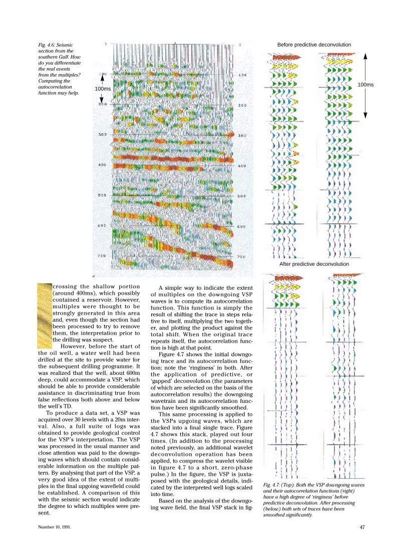
Figure 4.14 summarizes one field
acquisition arrangement, which is a
common one for obtaining offset (com-
pressional wave) VSP images in several
directions around the well. Multiple
shooting positions, at least 45° apart and
offset from the well by perhaps half the
tool depth, are occupied by vibrators. In
the well, the ASI is positioned over the
reservoir formations. A series of sweeps
from each source generates sufficient
data to compute VSPs for each source
azimuth. For better resolution of veloci-
ty differences, the sources could be
rotated around the well, or more
sources could be used.
What should the interpreter do next
with the VSP data to reach a reliable
conclusion about possible fracture
trends? Shear amplitudes may hold
information but are easily affected by
many other factors, in and outside the
borehole.
The angles at which the shear waves
arrive at the tool may also indicate
transmission differences, and can be
determined by careful measurements of
receiver orientations and intercept
angles.
Also, the analysis of how the direc-
tions of shear particle motion change
with time, even using data from a single
source, may be used to deduce fracture
trends. However, one familiar property
of shear waves is fairly easily accessible
Fig. 4.14: IN SEARCH OF
FRACTURES: Typical field
acquisition arrangement
for seismic fracture
surveys. The two vibrator
sources are positioned at
least 45° apart. The ASI
tool can record VSPs for
each source azimuth and
from this data it may be
possible to deduce the
presence and direction of
fractures.
Inversion of P and SV waves from Multicomponent
Offset Vertical Seismic Profiles by C. Esmersoy, in
Geophysics, v. 55, January 1990.
and can be measured robustly - their
velocity.
This approach is feasible because of
recently-developed processing algo-
rithms (see reference below) for sepa-
rating and inverting wave modes (to log-
like velocity functions).
Fracture directions
•
• • •
•
• • •
•
• • • • •
• • • •
• • •
• • • • • • •
•
• • •
•
• • •
•
• •
• •
•
• •
•
•
• • • •
• • •
• •
Offset -1 shear velocities
Off
set
-2 s
hea
r ve
loci
ties
5000
6400
7800
9200
10600
12000
5000 6400 7800 9200 10600 12000
Wireline (Armored
cable)
Cartridge
Bridle cable
Triaxial Sensor
Packages
50 ft
fig 3.3a TRY projection fig 3.3c HMX projection
ASI
Inversion
52 Middle East Well Evaluation Review
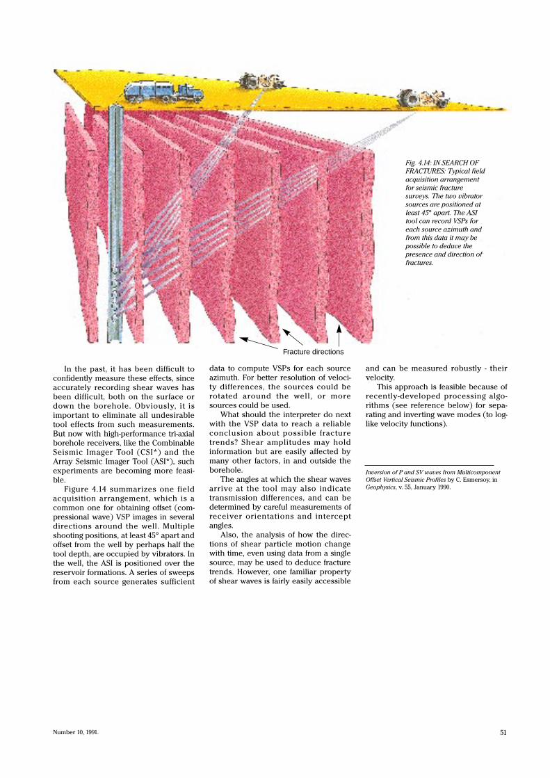
Figure 4.15 indicates how this proce-
dure works. The initial sections are pro-
duced from combined processing of the
vertical axis’ data and the wavefield cre-
ated from the projection of the horizon-
tal axes’ data in the direction of maxi-
mum horizontal particle motion - which
is mainly toward the sources (MiddleEast Well Evaluation Review, Number 4,1988).
The resultant compressional and
shear VSPs are then inverted to deter-
mine their velocities as a function of
depth. This is done for each direction
and these results can be compared by a
simple method such as cross-plotting.
This readily shows up variations over
particular depth zones. Differences of
about 3% to 4%, in shear velocities, have
been noted in such studies in the
Middle East. In projects now underway
these velocity variations, and other
shear wave attributes, are being corre-
lated with, among other things, fracture
density and orientation. These studies
require complete log data sets, includ-
ing Formation MicroScanner data (for
fracture logging), and borehole ovality
results, to indicate in situ stress fields.
Fig. 4.15:
Processing
steps involved
in the analysis
of tri-axial
shear wave
data.
DEPTH
ON
E-W
AY T
IME
(S
)
0.1
0.2
0.3
0.4
0.5
0.6
0.7
0.8
0.9
1.0
1.1
DEPTH
ON
E-W
AY T
IME
(S
)
0.1
0.2
0.3
0.4
0.5
0.6
0.7
0.8
0.9
1.0
1.1

53Number 10, 1991.
Track that crack
Besides recording the wavefields
transmitted from seismic sources,
the new high-performance, three-
component tools are being used
to address a very different prob-
lem: determining the extent of
hydraulically-induced fractures.
This technique essentially con-
sists of positioning the CSI or ASI
tool in or near a well undergoing
hydrofracturing, and ‘listening’ for the
acoustic signals generated when the
rock bursts.
The field operation is shown in figure
4.16. In order to increase a field’s pro-
ductivity, fluid is injected into the reser-
voir through perforations in the well’s
casing. The object is to overcome the
ambient pressure at this depth holding
the natural fracture planes together, and
force them apart. The most likely direc-
tion in which these fractures will open
up is at right angles to the minimum
stress direction, which is the direction
in which the force holding the fractures
together is least.
While this is going on, three-compo-
nent recordings can be made, either in
the injection well or in an adjacent well.
The orientation of these tools must be
determined before the recording, either
from orientation tools attached to them,
or by offset shot points, as shown in the
figure. The angle of incidence of the
Fig. 4.16: BIRD’S EYE VIEW: Field
acquisition set up for determining
the extent of hydrofracturing.
Fluid is pumped into a well to
induce fracturing. The fractures
open in the direction of maximum
stress (ie. at right angles to the
minimum stress direction).
At the same time, three-
component recordings can be
made to determine the orientation
of the borehole seismic tool.
The signals from the wave
fronts arriving at the axes of the
three-component array can be
cross-plotted against each other to
determine their arrival angle
relative to the tool’s sensors. The
different particle directions of the
different modes (compressional,
shear) should be recognizable in
this analysis.
waves from these shot points, which
have a known location, can be deter-
mined and used to find the alignment of
the tool’s horizontal axes.
The process for doing this is shown
on the right side of the figure. The
wavefronts received at the tool’s hori-
zontal axes will have a particular phase
depending upon the specific angle.
Plotting one axis’ response against the
other’s gives a type of cross plot. The
direction of this plot indicates the
wave’s angle across the array, and since
the alignment of the array has been
determined from the check shots (for
which the same procedure was used)
we know the true direction that the
wave is travelling in. In the figure, the
compressional event is the main plot,
and the later-arriving shear wave would
produce a plot roughly at right angles to
the compressional’s.
After many of these events have
been recorded and analysed in this
way, they can be compiled for each well
and tool position. When this is done in
the injection well, where particle
motion is in the plane of the fracture,
the fracture’s azimuth can be deter-
mined. When obtained from an adja-
cent well, the direction to the source is
indicated, and thus intersections can be
obtained for multi-well data sets.
Development work is continuing
with this kind of data. More information
on fracture height and width are being
sought from amplitudes and from the
differences in compressional and shear
arrival times.
Minimum stress
Wells
Minimum stress
Maximumstress
Maximumstress
3-componentgeophonearray
Compressionalwaves
Shear waves
Offsetshotpoints
x
x y
yShear wave
Direction of wave
z

54 Middle East Well Evaluation Review
Sharpening shears
The growing interest in shear wave seis-
mic data has placed a new demand on
sonic logging tools: how to get high-
quality, continuous shear waves, even
in shallow, low velocity rocks? Such
results are important, because complete
shear logs are critical for tying, in time,
logs to shear seismic sections.
A new tool which accomplishes this
feat in a novel fashion is the Dipole
Shear Sonic Imager Tool (DSI*).
Previous sonic tools used monopole
acoustic sources, which pulsed sym-
metrically outward from the tool (figure
4.17a). The compressional wave created
by the source was partially converted
into a shear wave at the borehole, if the
shear velocity in the rock was suitably
high. The dipole source, however, oper-
ates like a piston and produces an
asymmetric pressure field (figure 4.17b).
This pressure field flexes the borehole
wall back and forth, and directly creates
a shear-like wave travelling up the hole.
The wave is detected by an array of
receivers and wave slowness is mea-
sured by techniques developed in pre-
vious arrayed sonic tools (Middle EastWell Evaluation Review, Number 8,1990). Also, by having two pairs of
these transmitters at 90° to each other,
the shear wave velocity can be mea-
sured simultaneously in two directions.
Compressional waves are also created
and measured at the same time.
The dipole tool has another strength
- improved Stoneley wave measure-
ments, thanks to a special low frequen-
cy (monopole) transmitter. The useful-
ness of Stoneley waves for detecting
open, producing fractures in formations
was described in ‘Profiling
Permeability’ in Middle East WellEvaluation Review, Number 5, 1988.
This technique is now enhanced with
the new tool, and estimates of fracture
width can even be made.
Figure 4.18 is an example data set,
combined with an interpreted FMS
image which has fracture strikes and
dips noted. The Stoneley wavefield
shows strong reflections off the open
fractures (reflecting upwards when the
tool is above the fracture and down-
wards when it is below). Processing and
interpretation of the reflected Stoneley
events can indicate the fractures’ reflec-
tion coefficient and their degree of
openness.
Fig. 4.18: Detection of fractures with Stoneley waves from DSI: Low frequency
Stoneley waves reflect off open fractures in the formation, creating the chevron
pattern in the wavefield on the right. An analysis and interpretation of the strength of
the reflected events produces a ‘Stoneley reflection coefficient’ log, indicating the
extent and openness of the fractures. Correlation with the FMS interpretation (left)
confirms the sonic results.
Fig. 4.17a: Monopole source. Fig. 4.17b: Dipole source.

55Number 10, 1991.
to the right is the offset VSP, after pro-
cessing with all three of the tool’s com-
ponents. The section has thus had shear
events separated from the compression-
al. The shear might have distorted the
continuity of the events and made the
interpretation difficult. In this case, we
can see details of the formations’ conti-
nuity, and discontinuity, out to more
than 700m in the direction of the source.
Hole in one
Geophysicists can never get ‘good
enough’ data. Especially in the bore-
hole, good data can be hard to come by
with the seismic sensor suspended
beneath several miles of wire, tempera-
tures over 300°F and with the adjoining
formation crumbling away. And on top
of these factors, an entire drilling rig is
standing by, waiting. The ideal for
drillers is to minimize this time in the
hole, by using more receivers or by
adding other tools.
The answer to these demands is the
Combinable Seismic Imager, or CSI*
tool. Its key feature is the separate sen-
sor package which totally decouples
the gimbaled, tri-axial geophones from
the tool’s mass. Therefore, no matter
what is added to the tool, the seismic
signals will be unaffected.
This has several important implica-
tions. It is sometimes necessary to
know the orientation of the horizontal
receivers, so that the direction of
incoming seismic waves can be deter-
mined. Two such examples are dis-
cussed in this article - monitoring
acoustic emissions, and determining
the azimuths of shear waves. This need
also arises when recording reflections
in wells adjacent to features such as
fault planes or salt domes.
With the CSI, an orientation tool can
be added with no degradation of the sig-
nal. Another important use is in horizon-
tal wells. The CSI can be added to the
drill stem for operation horizontally, and
still receive high-quality seismic wave-
forms. Finally, to speed-up the acquisi-
tion of offset and walkaway VSPs, several
CSIs can be combined, to significantly
reduce the number of separate tool posi-
tionings. Figure 4.19 shows the basic fea-
tures of the tool.
CSI tools are now being used
throughout the Middle East. One impor-
tant application for the tool in Egypt,
where it has been used for more than
one year, is in obtaining high-quality
seismic images away from the borehole,
using offset and walkaway VSP tech-
niques (Middle East Well EvaluationReview, Number 1 1986). These images
can indicate, with greater precision than
that of surface seismic sections, the lat-
eral changes in formations identified in
the well.
Figure 4.20 is one such data set
acquired in Egypt. The left side of the fig-
ure shows the well’s geology and petro-
physics, based on Elemental Log
Analysis (ELAN*) processing of the logs;
Telemetry Combined tools
Extended sensor module
Shaker
Gimballed geophones
Isolating spring
CSI array
Fig. 4.20 (Above): Offset VSPacquired with the CSI tool.The well’s logs have beenused to compute an ELAN,which has been convertedinto time and is aligned withthe VSP’s seismic events.This allows the formationsand reservoir features to betracked in detail out from thewell.
ELAN
Acousticimpedance
log
Distance out from well
Two-
way
tim
e
Fig. 4.19: Basicfeatures of theCSI tool.
100m
s