Embed Size (px)
Citation preview

Mixed Layer Models
Observational Seminar – April 17, 2009

Two types of mixed layer models
Bulk mixed layer models:• PWP (Price et al., 1986)• bulk or slab models attempt to model the ML in an integral
sense - integrate governing equations over the mixed layerand balance quantities over the entire ML
Turbulence closure models:• 1st order - KPP• 2nd order - Mellor-Yamada• employ turbulence closure schemes that parameterize or
model higher-order turbulence moments

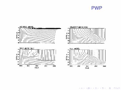
PWP
PWP is a bulk shear instability model• in PWP, the mixed layer, hm, is the minimum depth required
to keep a bulk Richardson number of a well-mixed layergreater than a prescribed critical value
• all properties are perfectly mixed in the mixed layer• below the mixed layer, properties are mixed to satisfy a
local gradient Richardson number criterion

PWP
For each forcing step, PWP:• applies surface momentum and heat fluxes to the surface
layer• mixes progressively deeper to ensure ∂ρ/∂z > 0• diagnoses the mixed layer depth, h, with a gradient method• determines whether the layer below the mixed layer is
entrained by calculating a bulk Richardson number:
Rib =g∆ρh
ρ0(∆Uj∆Uj)(1)
• if Rib < 0.65, the mixed layer entrains the layer below - allproperties are mixed in the mixed layer, and Rib iscalculated again - repeats until Rib > 0.65

PWP
• PWP then performs gradient Richardson number mixingbelow the mixed layer – calculates Rig for all layersbetween the base of the ML and the profile bottom
Rig =gδρ/δz
ρ0(∂V/∂z)2 ≥ 0.25 (2)
• if a level with Rig < 0.25 is found, PWP mixes in the twoneighboring points, then recalculates Rig - repeats until alllevels meet the criterion - this smears the sharp gradientsat the base of the mixed layer
• calculates mixed layer depth again and homogenizeswithin the mixed layer
PWP

Monin-Obukhov
Monin-Obukhov similarity theory is a popular boundary layerscaling. The important turbulence parameters are the distancefrom the boundary, d, and the surface kinematic fluxes, wx0.These apply for d < εh, where h is the boundary layer depthand ε << 1.• friction velocity: u*2 = w~u0 = |τ0|/ρ0
• turbulent fluctuation scales: θ*= −wθo/u*• Monin-Obukhov length scale: L = u*3/κFo
• L is the depth at which turbulence suppression by stablebuoyancy forcing (Fo > 0) balances mechanical production- larger F leads to shallower L
• friction velocity is a measure of the turbulent surface stress

KPP
The K profile parameterization (KPP) mixed layer model wasdeveloped from atmospheric boundary layer models thatincorporated nonlocal transport terms in their mixingparameterizations (Large et al., 1994).• nonlocal transport includes coherent structures like vertical
buoyant plumes, Langmuir cells, Kelvin-Helmholtzinstabilities, and internal gravity waves
• turbulent transports at a given level do not depend only onthe local property gradients at that level, but also on theoverall state of the boundary layer - such as the surfacefluxes and depth of the boundary layer
• velocity shear and stratification can exist in the ML• double diffusion, internal waves, and scale shear instability
contribute to eddy mixing coefficients in the interior

KPPFirst moment models like KPP assume a form for turbulentdiffusion: downgradient, depends linearly on the local propertygradient, with an eddy diffusivity Kx
wx(z) = −Kx (∂zX − γx ) (3)
• w is the velocity due to unresolved turbulent eddies and xis a property (like salinity)
• Kx values are nonlocal vertical mixing coefficients thatdepend on depth in the boundary layer, the depth of theboundary layer, and the surface forcing
• Kx acts on local property gradients to produce downgradient transports
• for unstable forcing, γx , the nonlocal transport term, canproduce counter gradient fluxes – γx is proportional to thesurface flux and inversely proportional to vertical frictionvelocity and ML depth

KPP
Profiles of buoyancy and buoyancy flux in a convectiveboundary layer:
• variation in mixed layer• h is the depth of the boundary layer• as d approaches the surface, the fluxes
linearly approach their surface value• nonlocal behavior - counter gradient
heat flux is evident as upward buoyancyflux in regions with constant orincreasing buoyancy with height (d/hbetween 0.35 and 0.8)

KPP - diffusivityLarge et al. first consider the diffusivity, Kx , in determining theturbulent diffusion:
wx(z) = −Kx (∂zX − γx ) (4)
The profile of boundary layer diffusivity is expressed as theproduct of the depth depended turbulent velocity scale, wx (σ)and a non-dimensional vertical shape function G(σ):
Kx (σ) = hwx (σ)G(σ) (5)
• σ = d/h, a nondimensional vertical coordinate in theboundary layer
• Kx is directly proportional to h because deeper boundarylayers can contain larger, more efficient turbulent eddies
The shape function is assumed to be a cubic polynomial:
G(σ) = a0 + a1σ + a2σ2 + a3σ
3 (6)

KPP - diffusivityThe constants in G(σ) are used to control diffusivities and theirvertical derivatives at the top and bottom of the boundary layer.Examples of normalized turbulent velocity scale, wx (σ)/κu*and G(σ): • turbulent eddies can’t cross boundary at d
= 0, so a0 = 0.• in the surface layer, σ < 0.1 and
G(σ) ≈ σa1, so a1 is set to be consistentwith Monin-Obukhov similarity theory
• turbulent velocity scales are functions ofh/L
• under unstable forcing (h/L<0) theturbulent velocity scales maintain theirσ = ε value in the boundary layer andmomentum and scalars mix differently(scalar dashed line)

KPP - diffusivity
• In KPP, the ocean interior can also forcethe boundary layer – a2 and a3 are chosenso that interior and boundary layer mixingcoefficients and their vertical derivativesmatch at d = h (σ = 1)
• shape function G(σ) can be different forscalars and momentum

KPP - nonlocal transport
wx(z) = −Kx (∂zX − γx ) (7)
Nonlocal transport, γx , is nonzero only for scalars in unstable(convective) forcing conditions. From Mailhot and Benoit(1982), it is parameterized as:
γs = Cswso
ws(σ)h, γθ = Cs
wθo + wθR
ws(σ)h, (8)
• γx is proportional to the surface fluxes and inverselyproportional to turbulent velocity scales and boundary layerdepth
• contributes to counter gradient fluxes• wθR represents radiative heat absorbed in the boundary
layer

KPP - boundary layer depthh, the depth of the boundary layer, is the depth to whichturbulent boundary layer eddies can penetrate vertically beforebeing stopped by stratification. h depends on the surfaceforcing, the oceanic velocity profile ~u(z), the buoyancy profile,and a parameterized turbulent velocity shear. KPP uses a bulkRichardson number criterion to determine h:
Ric =(Br − B(h))h|~ur − ~u(h)|2 + V 2
t(9)
• Br and ~ur are averages over the surface layer• V 2
t is the unresolved turbulent velocity shear – it is mostlyimportant when there is not enough wind to produce shearand is formulated to make model entrainment agree withtheoretical arguments and observations
• empirically determine critical value Ric = 0.3• turbulent eddies can penetrate much deeper than the ML

KPP - interior
Double diffusion, internal waves, and scale shear instabilitycontribute to eddy mixing coefficients in the interior (d > h):
νx (d) = νsx (d) + νw
x (d) + νdx (d) (10)
• momentum and scalars have different diffusivities for eachmechanism
• shear instability diffusivity, νsx , is parameterized as a
function of local gradient Richardson number• νw
x is constant• νd
x is parameterized as a function of the density ratio

KPP - testsLarge et al. test KPP in cases examining convection, winddeepening, diurnal cycling, and the annual cycle.

KPP - tests
KPP is successful at integrating timescales spanning 4 ordersof magnitude, from hours to years. It has trouble withrestratification.

KPP
Benefits of KPP:• allows structure in the mixed layer• interior mixing influences the turbulence throughout the
boundary layer (coupled at d = h)• boundary layer can penetrate interior stratification• realistic exchange of properties between the mixed layer
and the thermocline - distributes properties properly in thevertical
• insensitive to vertical resolution - good for long termclimate modeling

Second Order Closure Models
Second order turbulence closure models directly calculate thetime evolution of at least one second order moment. They try toinclude the turbulence generated by breaking surface gravitywaves and the Stokes production term, among other things.• Mellor-Yamada 2.5 is popular• second order closure methods are computationally
expensive• results are not proven to be better - they are known to have
too little entrainment during convection and too little mixingacross stabilizing density gradients