Media Mix Modeling vs. ANCOVA

An Analytical Debate

2

What is the best way to measure incremental sales, or “lift”, generated from marketing

investment dollars?

Measuring ROI From Promotional Spend

June July August September October November December

Where possible to implement, an experimental design that uses a randomly selected holdout group provides the most statistical power and reliability in marketing measurement

3

TMS

DM1

DM2

TMS

EM1

TMS

EM 2

Event

DM3 DM4

Sample Direct Marketing Campaign Plan: 2012

Market Events and External Factors

4

• Holdout sample should be selected from the lowest level of the experimental design and each treatment cell should have a corresponding randomly selected holdout group

Segment 1 Targets N=150,600

Segment 2 Targets N=350,200

Segment 3 Targets

N=102,000

RANDOM CONTROL

RANDOM CONTROL

RANDOM CONTROL

Sample Size Calculator

Use Randomization to Increase Statistical Power

TREATMENT GROUP (TEST)

TREATMENT GROUP (TEST)

TREATMENT GROUP (TEST)

NOTE: Control group can be much smaller than treatment group. Use sample size calculator to determine minimum possible sample size for control group

Option to apply finite population

correction adjustment

Verify Pre-Campaign Holdout Validity

• Random selection of the control group from the target group should guarantee that the test and control groups are equivalent on key metrics prior to the campaign start, but…

• Statistical testing of the difference between pre-period test and control groups on key metrics is an important validation step and adds to confidence in the post-period measurement

5

Sample Metrics Group1 Group2 Group3

Avg. Sales$ .45 .52 .35

Media Impressions .82 .84 .61

Other Promotional Spend

.25 .38 .27

Competitor Spend .31 .45 .24

Demographics .28 .19 .24

P-Values for the Difference Between Test and Control Group Mean Values on Key Metrics in Pre-Period

PRE PERIOD CAMPAIGN RUNS POST PERIOD

Pre-Period Trends: Test and Control Groups

p >.15 is non-significant

Test

Control

Sales by Week: Test and Control Groups

Measure Pre-Post Launch Change

• If the test group and control group are statistically equivalent prior to the campaign launch, then the difference in sales between the groups after the campaign represents the incremental sales contribution of the campaign

• ANCOVA (Analysis of Covariance) test will measure the significance of the difference and also control for other potential factors that could differentially impact test and control groups during the campaign period

6

PRE PERIOD CAMPAIGN POST

Campaign Effect ??

Pre-Period Post-

Period

Growth From Pre to Post

Test 0.45 0.65 0.20

Control 0.44 0.50 0.06

Test-Control 0.01 0.15 0.14

ANCOVA Adjusted 0.11

-

0.10

0.20

0.30

0.40

0.50

0.60

0.70

Average Weekly Sales per Target: Test v Control, Pre and Post

Campaign Effect

ANCOVA Adjusted difference is after controlling for covariates and, if significant (p-value less than .15), is the measure of true incremental sales from the campaign

Summary: ANCOVA for Marketing Measurement

Benefits

• Extremely reliable results

• Conservative test

• Control for other factors that may impact volume growth of target relative to holdout

• Able to scale to calculate overall ROI from marketing program

• Expect replicable results if same conditions and weights apply in repeated treatment

7

8

There is another option…

Media Mix Modeling can overcome many limitations of ANCOVA-based analysis

Limitations of ANCOVA

• Feasibility of holdout group

• Opportunity cost of being out of market with incremental media

• Selection of test period length is subjective

• Difficult to measure mass & digital media

• No guidance on cross-tactic decisions

• Does not provide insight into future budget allocation decisions

• Does not explain “base” factor contributions

9

As we will see, Media Mix Modeling will overcome all of these limitations…

How is Media Mix Modeling Different?

10

Media Mix Models can be used to understand the incremental, layered effect of cross-tactic marketing over time…

Base

Incremental Media Contribution

What are the Requirements and Process?

Time

Investment

0

10

20

30

40

50

60

1 3 5 7 9 11 13 15 17 19 21 23

Re

ven

ue

Time

Sales Decomposition

TV

Direct Mail

Radio

Print

Base

Base51%

Print14%Radio

8%

Direct Mail11%

TV16%

Segment 1

0

20

40

60

80

100

120

140

160

180

200

0.0 24.0 48.0

Incr

em

en

tal R

eve

nu

e

Investment Amount

Print

Radio

Direct Mail

TV

0

20

40

60

80

100

120

140

160

180

200

0.0 24.0 48.0

Incr

em

en

tal R

eve

nu

e

Investment Amount

Print

Radio

Direct Mail

TV

0

50

100

150

200

250

300

350

0 5 10 15 20 25 30

Time

TV

0

200

400

600

800

1000

1200

0 5 10 15 20 25 30

Time

Direct Mail

0

50

100

150

200

250

0 5 10 15 20 25 30

Time

Radio

0

20

40

60

80

100

120

140

160

180

0 5 10 15 20 25 30

Time

Print

p

i

t

p

ititixy

1

-

100

200

300

400

500

600

Segment 1 Segment 2

280 298

73 73 42 46 62 49

87 71

Re

ven

ue

TV

Direct Mail

Radio

Print

Base

11

Input Data Statistical Models Response Curves & Optimization

How Does Media Mix Modeling Work?

12

L

l

ltlt Xy1

0

2

12110 xxy

110 xy

k

Lxxy ...1

10

k

Lxxxy ...21

210

n

i

i

n

i

ii

ii

xx

yyxx

xy

1

2

11

10

)(

))((ˆ

ˆˆ

iiiii xyyyu 10ˆˆˆˆ

2

1

10

1

2 )ˆˆ(ˆn

i

ii

n

i

i xyu

Functional forms of model equations… Estimation of equations…

)exp(1

10

xy

Functional Forms of Equations

• Functional form of a relationship between response and explanatory variables is determined by factors such as diminishing/increasing returns to scale, (a)symmetry in response, etc.

• Some of the most frequently used functional forms are:

Functional Form Representation Return to Scale

Linear

Constant

Quadratic

Diminishing

Power additive

Diminishing

Multiplicative (log-log)

Diminishing

Log-Reciprocal

S-Shaped

13

L

l

ltlt Xy1

0

2

12110 xxy

110 xy

k

Lxxxy ...21

210

)exp(1

10

xy

Estimation of Equations

• Example equation

• Estimation of the ‘betas’

• Residual

• Sum of Squared Residuals

iii uxy 10

n

i

i

n

i

ii

ii

xx

yyxx

xy

1

2

11

10

)(

))((ˆ

ˆˆ

Sample covariance between x and y divided by the sample variance of x

Intercept equals the sample average of y plus the sample estimate of x

iiiii xyyyu 10ˆˆˆˆ Difference between actual and predicted, estimate of

the unknown error in the population equation

Population equation indicating relationship between x and y; estimated using sample of data representing the population

2

1

10

1

2 )ˆˆ(ˆn

i

ii

n

i

i xyuOrdinary Least Squares estimates minimize the sum of squared residuals

14

Application of Parameter Estimates

• How do we calculate contribution for each variable in the model?

– Multiply coefficient from model (“beta”) by weekly model inputs (impressions)

– Sum weekly values to get total contribution attributable to each media

• Model Coefficient (“Beta”) for Display: 0.0000486431

Week

Display Impressions

Contribution

5/30/2009 1,972,606 96

6/6/2009 2,226,734 108

6/13/2009 2,483,358 121

…

5/7/2011 5,550,921 270

5/14/2011 7,016,425 341

5/21/2011 4,937,705 240

Sum contribution across weeks to get total incremental sales due to Display… 53,415

15

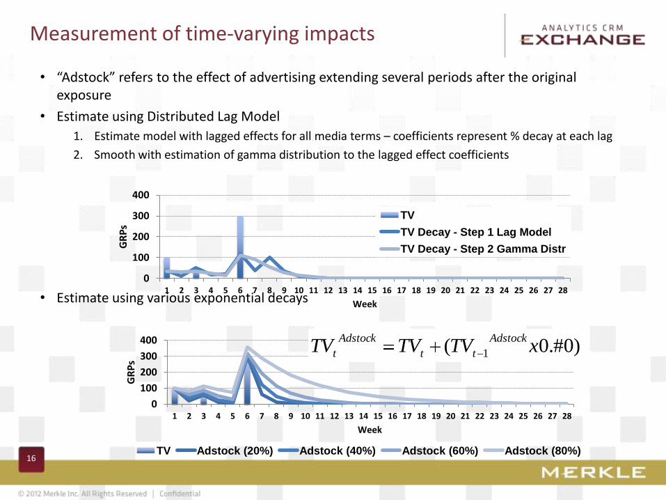
• “Adstock” refers to the effect of advertising extending several periods after the original exposure

• Estimate using Distributed Lag Model

1. Estimate model with lagged effects for all media terms – coefficients represent % decay at each lag

2. Smooth with estimation of gamma distribution to the lagged effect coefficients

• Estimate using various exponential decays

Measurement of time-varying impacts

16

0

100

200

300

400

1 2 3 4 5 6 7 8 9 10 11 12 13 14 15 16 17 18 19 20 21 22 23 24 25 26 27 28

GR

Ps

Week

TV Adstock (20%) Adstock (40%) Adstock (60%) Adstock (80%)

)0.#0( 1 xTVTVTVAdstock

tt

Adstock

t

0

100

200

300

400

1 2 3 4 5 6 7 8 9 10 11 12 13 14 15 16 17 18 19 20 21 22 23 24 25 26 27 28

GR

Ps

Week

TV

TV Decay - Step 1 Lag Model

TV Decay - Step 2 Gamma Distr

Methodologies used in MMM Analyses

– Ordinary Least Squares (OLS)

– Mixed (Bayesian Shrinkage, Random Coefficients)

– Unobserved Components Models (UCM)

– Two Stage: UCM-Mixed

– Seemingly Unrelated Regression (SUR)

– Structural Equation Modeling (SEM)

Toolset of econometric methodologies

17

Time Series Data

(i.e. National x Week)

Panel Data (i.e. DMA x Week)

Hierarchical Relationships

OLS UCM Mixed

Two Stage: UCM - Mixed

SUR SEM

Methodology Selection

18

Case Study Comparisons

What does each approach offer in these instances?

Case Study 1: Direct Campaign

• Typical multi-channel campaign to physicians with mix of tactics deployed in rapid succession across long timeframe

• Capitalizes on use of “universal control group” of non-marketed holdout

19

-

0.05

0.10

0.15

0.20

0.25

0.30

0.35

0.40

0.45

NR

x p

er

Ph

ysic

ian

pe

r W

ee

k

EM1 Resend 1

EM1 Resend 2

DM2 EM1 EM2

EM2 Resend 1

DM1 DM2 Tele-detail

Case Study 1: ANCOVA APPROACH

1. Define multiple pre-post periods

2. Conduct holdout-validity tests for each pre-period and each set of test/control groups

3. Measure ANCOVA-Adjusted change in volume using double difference

20

-

0.05

0.10

0.15

0.20

0.25

0.30

0.35

0.40

0.45

NR

x p

er

Ph

ysic

ian

pe

r W

ee

k

EM1 Resend 1

EM1 Resend 2

DM2 EM1 EM2

EM2 Resend 1

DM1 DM2 Tele-detail

ANCOVA: PRE

PERIOD 1

ANCOVA: POST

PERIOD 1

PRE PERIOD 2 POST PERIOD 2

Case Study 1: ANCOVA

Change in Per Physician Prescription Volume from Pre1 to Post 1

Change in Volume from Pre2 to Post2

Test +1.4 +2.5

Control +0.4 -0.2

Difference 1.0 2.7

ANCOVA-Adjusted 0.8 2.2

Significance .05 p <.001

• ANCOVA could provide solid measurement of overall campaign impact for two different time periods while controlling for other factors

• Per physician increase could be scaled to measure total impact and calculate overall ROI

21

Ancova 1: Time Period 1 Ancova 2: Time Period 2

Case Study 1: Mixed Modeling Approach

22

1. Use correlogram approach fitted with gamma curves to calculate decay curves per channel

2. Transform input variables to account for decay

3. Build model at the physician-week level over 130 weeks of history and all physicians, whether targeted or not in campaign

4. Fit model using best functional form

5. Calculate response curves for each tactic

6. Input into planning tool for optimization

Case Study 1: Campaign Planning From MMO Output

23

• MMO equation creates outputs that can be used in a scenario planning tool to test the impact of different investment levels by tactic and calculate expected ROI from varying budget levels

… and ANCOVA confirmed lift estimates

Case Study 2: Web Support Program

24

• Situation: Launched consumer support website where consumers register online for product support and information. Consumers only provide zip code in online support registration. Sales not able to be tied directly to consumers but only to geography (zip code)

• Key question: Does consumer support program drive future sales?

- 0.10 0.20 0.30 0.40 0.50

Sep-09 Oct-09 Nov-09 Dec-09 Jan-10 Feb-10

Web Visits per HH per Month

Control

Test

-

0.05

0.10

0.15

0.20

Sep-09 Oct-09 Nov-09 Dec-09 Jan-10 Feb-10

Volume per household per month – Pre Launch

Control

Test

0%

5%

10%

15%

Sep-09 Oct-09 Nov-09 Dec-09 Jan-10 Feb-10

Market Share – Pre Launch

Control

Test

ANCOVA Approach: 1) Match consumer registered zip code

to most likely purchase zip code 2) Identify control zip codes with no

consumer registrations in proximity 3) Test “lift” after web program launches

Case Study 2: Possible ANCOVA Output

25

• Test pre-post period differences between zip codes with registrations and with no registrations

• Control for covariates that might influence test zip codes

ANCOVA may demonstrate a link between sales and web support program use

Case Study 2: Mixed Model Approach

26

Input Model ROI

Baseline 52%

TV GRP 25% 2:1

Registrations 3% 4:1

Activation 1 6% 3:1

Activation 2 7% 6:1

Promotion 1 7% 1:1

Effect Estimate StdErr tValue Probt

Intercept 0.126 0.009 13.433 0.000

log_trend 0.025 0.004 6.719 0.000

total_mkt_grp 0.411 0.012 35.333 0.000

sq_total_mkt_grp (0.139) 0.005 -27.309 0.000

decay_register 5.037 0.755 6.672 0.000

sq_decay_register (8.051) 2.934 -2.744 0.006

decay_activation1 7.056 0.550 12.820 0.000

sq_decay_activation1 (4.106) 1.586 -2.589 0.010

decay_activation2 0.603 0.077 7.823 0.000

sq_decay_activation2 0.052 0.040 1.297 0.194

Effect Estimate StdErr tValue Probt

Intercept 0.138 0.009 14.6 <.0001

log_trend 0.019 0.004 5.01 <.0001

total_mkt_grp 0.404 0.012 34.74 <.0001

sq_total_mkt_grp (0.137) 0.005 -26.84 <.0001

decay_register 4.763 0.754 6.32 <.0001

sq_decay_register (7.204) 2.931 -2.46 0.014

decay_activation1 7.055 0.550 12.83 <.0001

sq_decay_activation1 (4.368) 1.584 -2.76 0.006

decay_activation2 0.581 0.077 7.56 <.0001

sq_decay_activation2 0.057 0.040 1.44 0.151

decay_promotion1 0.123 0.009 13.2 <.0001

sq_decay_promotion1 (0.005) 0.001 -6.79 <.0001

Model Output: Quadratic Form

1. Collect zip-level data on all programs in place, by week, over long time period

2. Calculate contribution of each of the tactics, including the web registrations

3. Compare relative contribution to sales and relative ROI levels of each tactic

Case Study 3: Cross-Tactic Measurement

27

Base 43%

Contribution % FY 2010

Media mix modeling indicates incrementality of media along with indication of ROI across tactics…

20%

32%

5%

9%

55% 30%

7% 19%

8% 10%

5%

Spend % Increm. Sales %

Spend – Incremental Sales FY 2011

Streaming Video

Newspaper

Direct Mail

TV

Radio

Display

$200M

280

120

50

180

150

ROI Index

Incremental 57%

Situation: Large advertising spend – objective is to optimize spend by tactic and geography

Case Study 3: MMM provides insights into promotional performance by region

28

3% 3% 7%

13% 11% 13% 12% 17%

6% 9% 4%

9% 9% 10% 12% 11% 12% 14%

4% 4%

123

303

122 76

114 80 101 81 67

44

0%

10%

20%

30%

40%

50%

60%

70%

80%

90%

100% Promo Tactics by Region FY 2011

% Cost % Increm Sales ROI Index

Media mix modeling indicates promotional messaging is more effective in the Midwest than all other regions…

29

A Best Practice Approach

.. Taking marketing measurement to the next level

Comparison of Methods

= Winner on this Attribute

ANCOVA Media Mix Modeling

Cost (Depends on # groups)

Hidden Costs Cost of withholding promotion

from control

Complexity of Execution Statistics simpler, but test

design more complex

Data Requirements

Measurement Ability

Scenario Planning Only to repeat exact

Best for...

30

Best Practice Measurement Framework

31

Direct

•Creative •Segment

Display

•Creative •Site •Landing Page

DRTV

•Creative •Daypart •Duration

TV

•Creative •Daypart •Duration

Category

Measurement Level:

Media Vehicle

Tactic

1-800

Media Base

Search

•Site •Keyword

Measure using Indirect/Direct

Attribution • Last-click

• In-market testing (ANCOVA)

• Ad tracking

Measure using Media Mix Modeling

Media Mix Modeling gives best practice estimates of media impacts – both overall and at the vehicle level. The methodology is also extensible to the tactic level, and can be applied in cases where indirect or direct attribution is not feasible. Indirect/Direct Attribution is best employed in relative analyses within a media vehicle, at levels of granularity not possible via traditional mix modeling (i.e. search keywords).

Legend:

Brian Demitros

Associate Director

Integrated Media Optimization Practice

Merkle Analytics

443.542.4438 BDemitros@merkleinc.com

Lynda S Gordon

Senior Director

Life Sciences Analytics Practice

Merkle Analytics

440.476.0351

LSGordon@merkleinc.com

Merkle Analytics