MIT Joint Program on theScience and Policy of Global Change

Uncertainty in Emissions Projections forClimate Models

Mort D. Webster, Mustafa H. Babiker, Monika Mayer, John M. Reilly,Jochen Harnisch, Robert Hyman, Marcus C. Sarofim and Chien Wang

Report No. 79August 2001

The MIT Joint Program on the Science and Policy of Global Change is an organization for research,independent policy analysis, and public education in global environmental change. It seeks to provide leadershipin understanding scientific, economic, and ecological aspects of this difficult issue, and combining them into policyassessments that serve the needs of ongoing national and international discussions. To this end, the Program bringstogether an interdisciplinary group from two established research centers at MIT: the Center for Global ChangeScience (CGCS) and the Center for Energy and Environmental Policy Research (CEEPR). These two centersbridge many key areas of the needed intellectual work, and additional essential areas are covered by other MITdepartments, by collaboration with the Ecosystems Center of the Marine Biology Laboratory (MBL) at Woods Hole,and by short- and long-term visitors to the Program. The Program involves sponsorship and active participation byindustry, government, and non-profit organizations.

To inform processes of policy development and implementation, climate change research needs to focus onimproving the prediction of those variables that are most relevant to economic, social, and environmental effects.In turn, the greenhouse gas and atmospheric aerosol assumptions underlying climate analysis need to be related tothe economic, technological, and political forces that drive emissions, and to the results of international agreementsand mitigation. Further, assessments of possible societal and ecosystem impacts, and analysis of mitigationstrategies, need to be based on realistic evaluation of the uncertainties of climate science.

This report is one of a series intended to communicate research results and improve public understanding of climateissues, thereby contributing to informed debate about the climate issue, the uncertainties, and the economic andsocial implications of policy alternatives. Titles in the Report Series to date are listed on the inside back cover.

Henry D. Jacoby and Ronald G. Prinn,Program Co-Directors

For more information, please contact the Joint Program Office

Postal Address: Joint Program on the Science and Policy of Global ChangeMIT E40-27177 Massachusetts AvenueCambridge MA 02139-4307 (USA)

Location: One Amherst Street, CambridgeBuilding E40, Room 271Massachusetts Institute of Technology

Access: Phone: (617) 253-7492Fax: (617) 253-9845E-mail: gl o bal cha nge @mi t .e duWeb site: htt p://mi t .e du / glo bal change /

Printed on recycled paper

Uncertainty in Emissions Projections for Climate Models

Mort D. Webster1, Mustafa H. Babiker2, Monika Mayer3, John M. Reilly2,Jochen Harnisch4, Robert Hyman2, Marcus C. Sarofim2 and Chien Wang2

1Department of Public Policy, University of North Carolina Chapel Hill2Joint Program on the Science and Policy of Global Change, MIT3AVL List GmbH, Graz, Austria4ECOFYS energy & environment, Energy Technologies Centre (ETZ), Nuremberg, Germany

Abstract

Future global climate projections are subject to large uncertainties. Major sources of thisuncertainty are projections of anthropogenic emissions. We evaluate the uncertainty infuture anthropogenic emissions using a computable general equilibrium model of the worldeconomy. Results are simulated through 2100 for carbon dioxide (CO2), methane (CH4),nitrous oxide (N2O), hydrofluorocarbons (HFCs), perfluorocarbons (PFCs) and sulfurhexafluoride (SF6), sulfur dioxide (SO2), black carbon (BC) and organic carbon (OC),nitrogen oxides (NOx), carbon monoxide (CO), ammonia (NH3) and non-methane volatileorganic compounds (NMVOCs). We construct mean and upper and lower 95% emissionsscenarios (available from the authors at 1o x 1o latitude-longitude grid). Using the MITIntegrated Global System Model (IGSM), we find a temperature change range in 2100 of0.9 to 4.0 oC, compared with the Intergovernmental Panel on Climate Change emissionsscenarios that result in a range of 1.3 to 3.6 oC when simulated through MIT IGSM.

Contents

1. Introduction ......................................................................................................................................... 21.1 Uncertainty Analysis................................................................................................................... 3

An Economic Emissions Model.............................................................................................. 4Sensitivity Analysis ................................................................................................................. 6Probability Distributions of Uncertain Parameters ............................................................. 8The DEMM Approach .......................................................................................................... 13

1.2 Emissions Uncertainty Results ................................................................................................. 142. Scenarios for Climate Simulations ................................................................................................... 173. Climate Impacts of Representative Scenarios.................................................................................. 194. Conclusions ....................................................................................................................................... 22References ............................................................................................................................................. 23

1 Corresponding author: Department of Public Policy, University of North Carolina Chapel Hill, CB# 3435, Chapel

Hill, NC, 27599 USA; E-mail: mort@unc.edu, Telephone: (919) 843-5010.keywords: atmospheric chemistry, Monte Carlo simulation, air pollution, economic models, greenhouse gases, earth

systems modeling; submitted to Atmospheric Environment (July 2001)

2

1. INTRODUCTION

Many human activities cause the release of substances that alter the radiative properties ofthe atmosphere. Projections intended to represent plausible transient climate change due toanthropogenic forcing must, therefore, rely on emissions projections produced by models ofeconomic activity and technological change that determine the level of human activities andemissions rates from those activities. Such projections of changes in economic and technologicalforces are, however, subject to considerable uncertainty. The evaluation of uncertainty ineconomic and technological factors and the effects on forecasts of carbon dioxide emissions hasa relatively long history (e.g., Nordhaus and Yohe, 1985; Reilly et al., 1987) but the emissionsforecasts associated with particular uncertainty limits, heretofore, have not been used to forcecomplex climate models.

A major advance over the past decade has been the development of coupled ocean-atmosphere models combined with development of computational capacity to simulate transientclimate change (IPCC, 2001), and complex climate models are now at a state of developmentwhere they are capable of using emissions scenarios generated by economic models. A secondmajor advance on the atmospheric modeling front has been the coupling of atmosphericchemistry models with climate models so that the complex interactions of greenhouse gases,urban air pollutants, and other substances can be explicitly represented (Wang et al., 1998;Mayer et al., 2000). Economic modeling has made major advances as well, most recently in theability to consistently model and project the human activities that lead to emissions of the manysubstances that affect climate directly or indirectly (Babiker, et al., 2001; Reilly et al., 1999;IPCC SRES).

These advances in economic and climate modeling make it timely, therefore, to reconsideruncertainty in emissions projections. In this paper, we describe the development of a consistentset of emissions scenarios with known probability characteristics based on projections of humanactivities over the next 100 years.2 To produce these scenarios we make use of recentdevelopments in uncertainty techniques (Tatang et al., 1997) and apply them to the EmissionsPrediction and Policy Analysis (EPPA) model (Babiker et al., 2001), a computable generalequilibrium model (CGE) of the world economy that projects the major greenhouse gases aswell as other climatically or chemically important substances. We compare our results to thescenarios generated for the Intergovernmental Panel on Climate Change (IPCC) Special Reporton Emissions Scenarios (SRES, 1999).

The next section begins with a brief discussion of uncertainty analysis and details of ourapproach. We then present the resulting distributions of emissions. Finally, we develop specificemissions scenarios with known probability characteristics and simulate resulting climate changeusing the MIT Integrated Global Systems Model (IGSM), comparing them to the SRES resultsalso simulated through the MIT IGSM (Prinn et al., 1999; Reilly et al., 1999).

2 These scenarios are gridded at 1° x 1° latitude-longitude, and are available to interested researchers by contacting

the corresponding author.

3

1.1 Uncertainty Analysis

There are two broadly different ways to approach the problem of forecasting when thereis substantial uncertainty: uncertainty analysis (associating probabilities with outcomes) andscenario analysis (developing “plausible” scenarios that span an interesting range of possibleoutcomes). Both approaches are evident in climate assessments, most notably the recent IPCCreports. Authors for the IPCC Third Assessment Report (TAR) were provided guidanceencouraging them to move as far toward uncertainty quantification as possible. TAR authorswere asked to identify the most important factors and uncertainties likely to affect conclusions,document ranges and distributions in the literature, quantitatively (when possible) orqualitatively characterize the distribution of values that a parameter, variable or outcome maytake, and optionally to use formal probabilistic frameworks for assessing expert judgment(Moss and Schneider, 2000). The IPCC Special Report on Emissions Scenarios (SRES, 1999)uses the plausible scenario approach. The approach there was described as a “story line” analysiswhere all the scenarios developed were considered “equally valid,” the authors strongly resistingan assignment of quantitative or qualitative likelihoods to scenarios.

There can be great benefit to a “story line” approach as it allows one to explore in detail howparticular sets of assumptions produce different or similar outcomes. One advantage is that inassessments involving a set of authors with widely diverging views, it is typically easier topresent scenarios without attaching likelihoods. When there exist widely divergent “worldviews,” a term Edmonds and Reilly (1985) used to describe different views about future energyuse and carbon intensity, one expert’s likelihood range may not include another expert’s mostlikely scenario making it as difficult to reach consensus on a likelihood ranges as on a mean orbest guess case. A similar issue of consensus distributions also arises in expert elicitation in thecontentious issue of whether or how to combine the judgments of different experts (Keith, 1996;Pate-Cornell, 1996). The scenario or “story line” approach allows scenarios from experts withwidely varying “world views” to be considered “equally valid”, avoiding deadlock.

The alternative approach, uncertainty analysis, requires identification of the critical uncertainmodel parameters, quantification of the uncertainty in those parameters in the form of probabilitydistributions, and then sampling from those distributions and performing model simulationsrepeatedly to construct probability distributions of the outcomes. With this approach, one canquantify the likelihood that an outcome falls within some specified range.

In the end, the difference between formal quantitative uncertainty analysis and the story linescenario approach is not whether a judgment about likelihood of outcomes is needed but ratherwhen and by whom the judgment is made. Scientists can use the tools of uncertainty analysisand their judgment to describe the likelihood of outcomes quantitatively or the assessment oflikelihood can be left to those who actually must use the information; i.e. policy makers and thepublic who must ultimately decide whether the risks of climate change are great or small. Ourviews are that (1) it is important for experts to offer their judgment about uncertainty in theirprojections and (2) formal uncertainty techniques can eliminate some of the well-knowncognitive biases that exist when people deal with uncertainty (Tversky and Kahneman, 1974).The evidence is strong that experts and laymen are equally prone to such biases and quantitativeapproaches can reduce if not eliminate these biases (Morgan and Henrion, 1990).

4

A unique aspect of the uncertainty approach we use is that we are able to produce emissionsprojections that are consistent with underlying economic, demographic, and technologicalassumptions across substances for any year and over time. Choosing the 95% upper confidencelimit for CO2, SO2, and CH4 as derived from an uncertainty analysis, for example, will producea much more unlikely climate scenario than the 95% upper confidence3 limit on total radiativeforcing unless these emissions are perfectly correlated. We know, however, that coal mining andcoal burning are, for practical purposes, perfectly correlated at the global level and that coalmining releases CH4 and coal burning results in emissions of CO2 and SO2. Thus, we expectcorrelation in emissions of these three substances. The correlation is far from perfect, however,because there are other sources of all of these substances. Moreover, SO2 and CH4 emissions aresubject to control measures that do not effect CO2 emissions proportionately and both the sulfurcontent of coal and CH4 release from coals mines varies greatly across regions, weakening thecorrelation among these emissions.

There is also likely to be a correlation structure for distributions across time. For example, atime profile of energy consumption that exhausts much of the cheaply available oil and gas in thefirst half of the century may lead to much greater reliance on higher emitting coal and shale oil inthe latter half of the century whereas a time profile of energy consumption that relies on coal inthe first half of the century will have more lower emitting natural gas available in the second halfof the century.

Our method also allows us to recover the underlying parameter values that can lead toa particular case, where they lie in the input distributions we used, and the probabilitycharacteristics of the outcome associated with the case. By using this set of parameters, thescenario so constructed is consistent with the structure of the underlying model that includes thetechnological and economic relationships that create correlation among emissions and over time.In principle, one can then explore in detail the sensitivity of results to varying assumptionsaround such a case, allowing others to form different judgments about the likelihood, andconduct policy analysis using these cases as reference cases. While the set of parameter valuesassociated with a particular set of outcomes is not unique, our approach allows a more structureddevelopment of families of scenarios that could serve as a basis for “story line” type analysis.This approach offers greater assurance of having explored a range of outcomes that brackets aspecific likelihood range such as the 95 percent confidence limits.

Our approach involves: (1) choice of an appropriate model (2) sensitivity analysis todetermine those parameters that are most important for particular outcomes (3) development ofprobability distributions for the parameters chosen for analysis (4) application of theDeterministic Equivalent Modeling Method (DEMM) approach to produce a polynomial reducedform fit of the EPPA model (5) Monte Carlo simulation of the reduced form polynomial fitdeveloped using DEMM.

An Economic Emissions Model

The EPPA model is well suited for this task, as it was designed to simulate the worldeconomy through time with the objective of producing scenarios of greenhouse gases (GHGs)

3 Conditional on a specific set of climate model assumptions.

5

and their precursors, emitted as a result of human activities. The simulation horizon is throughthe year 2100, producing emissions scenarios for the major greenhouse gases (carbon dioxide(CO2), methane (CH4), nitrous oxide (N2O), hydrofluorocarbons (HFCs), perfluorocarbons(PFCs) and sulfur hexafluoride (SF6))

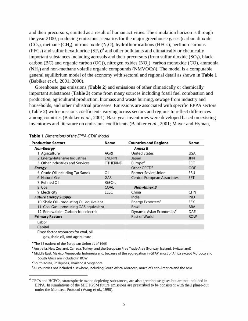
4 and other pollutants and climatically or chemicallyimportant substances including aerosols and their precursors (from sulfur dioxide (SO2), blackcarbon (BC) and organic carbon (OC)), nitrogen oxides (NOx), carbon monoxide (CO), ammonia(NH3) and non-methane volatile organic compounds (NMVOCs)). The model is a computablegeneral equilibrium model of the economy with sectoral and regional detail as shown in Table 1(Babiker et al., 2001, 2000).

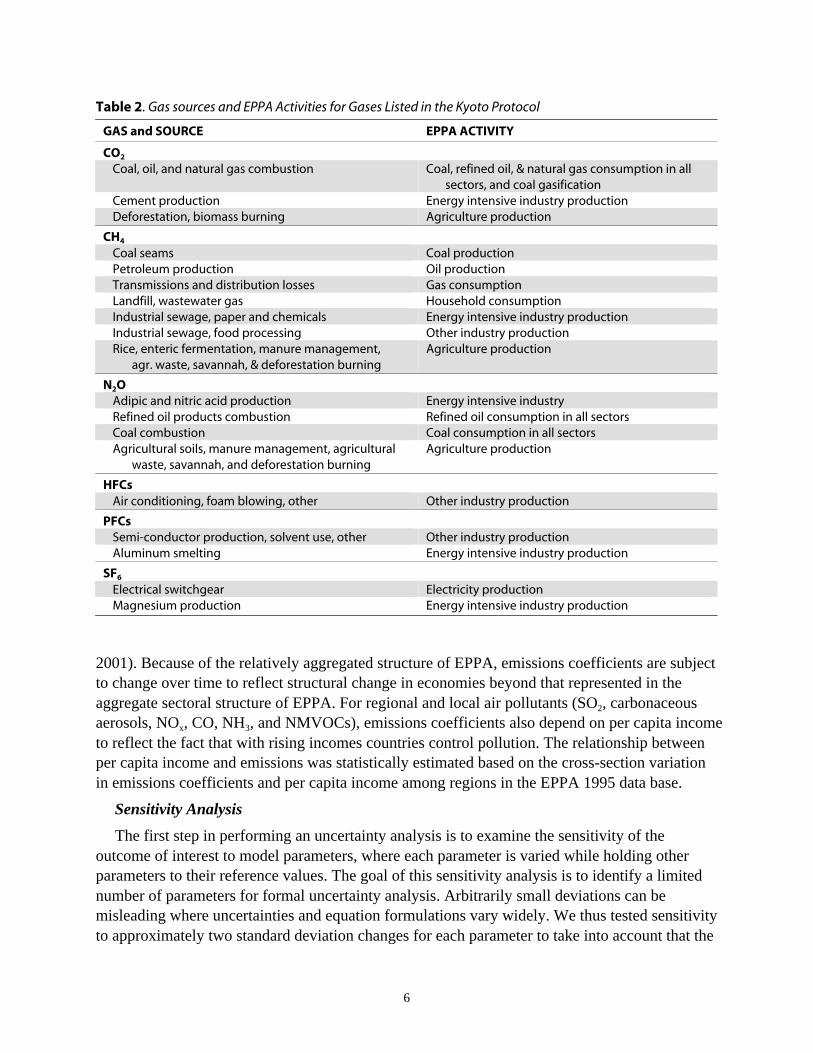
Greenhouse gas emissions (Table 2) and emissions of other climatically or chemicallyimportant substances (Table 3) come from many sources including fossil fuel combustion andproduction, agricultural production, biomass and waste burning, sewage from industry andhouseholds, and other industrial processes. Emissions are associated with specific EPPA sectors(Table 2) with emissions coefficients varying across sectors and regions to reflect differencesamong countries (Babiker et al., 2001). Base year inventories were developed based on existinginventories and literature on emissions coefficients (Babiker et al., 2001; Mayer and Hyman,

Table 1. Dimensions of the EPPA-GTAP Model

Production Sectors Name Countries and Regions Name

Non-Energy Annex B1. Agriculture AGRI United States USA2. Energy-Intensive Industries ENERINT Japan JPN3. Other Industries and Services OTHERIND Europea EEC

Energy Other OECDb OOE5. Crude Oil including Tar Sands OIL Former Soviet Union FSU6. Natural Gas GAS Central European Associates EET7. Refined Oil REFOIL8. Coal COAL Non-Annex B9. Electricity ELEC China CHN

Future Energy Supply India IND10. Shale Oil - producing OIL equivalent Energy Exportersc EEX11. Coal Gas - producing GAS equivalent Brazil BRA12. Renewable - Carbon-free electric Dynamic Asian Economiesd DAE

Primary Factors Rest of World ROW

LaborCapitalFixed factor resources for coal, oil,

gas, shale oil, and agriculturea The 15 nations of the European Union as of 1995b Australia, New Zealand, Canada, Turkey, and the European Free Trade Area (Norway, Iceland, Switzerland)c Middle East, Mexico, Venezuela, Indonesia and, because of the aggregation in GTAP, most of Africa except Morocco and

South Africa are included in ROWd South Korea, Phillipines, Thailand & SingaporeeAll countries not included elsewhere, including South Africa, Morocco, much of Latin America and the Asia

4 CFCs and HCFCs, stratospheric ozone depleting substances, are also greenhouse gases but are not included in

EPPA. In simulations of the MIT IGSM future emissions are prescribed to be consistent with their phase-outunder the Montreal Protocol (Wang et al., 1998).

6

Table 2. Gas sources and EPPA Activities for Gases Listed in the Kyoto Protocol

GAS and SOURCE EPPA ACTIVITY

CO2

Coal, oil, and natural gas combustion Coal, refined oil, & natural gas consumption in allsectors, and coal gasification

Cement production Energy intensive industry productionDeforestation, biomass burning Agriculture production

CH4

Coal seams Coal productionPetroleum production Oil productionTransmissions and distribution losses Gas consumptionLandfill, wastewater gas Household consumptionIndustrial sewage, paper and chemicals Energy intensive industry productionIndustrial sewage, food processing Other industry productionRice, enteric fermentation, manure management,

agr. waste, savannah, & deforestation burningAgriculture production

N2OAdipic and nitric acid production Energy intensive industryRefined oil products combustion Refined oil consumption in all sectorsCoal combustion Coal consumption in all sectorsAgricultural soils, manure management, agricultural

waste, savannah, and deforestation burningAgriculture production

HFCsAir conditioning, foam blowing, other Other industry production

PFCsSemi-conductor production, solvent use, other Other industry productionAluminum smelting Energy intensive industry production

SF6

Electrical switchgear Electricity productionMagnesium production Energy intensive industry production

2001). Because of the relatively aggregated structure of EPPA, emissions coefficients are subjectto change over time to reflect structural change in economies beyond that represented in theaggregate sectoral structure of EPPA. For regional and local air pollutants (SO2, carbonaceousaerosols, NOx, CO, NH3, and NMVOCs), emissions coefficients also depend on per capita incometo reflect the fact that with rising incomes countries control pollution. The relationship betweenper capita income and emissions was statistically estimated based on the cross-section variationin emissions coefficients and per capita income among regions in the EPPA 1995 data base.

Sensitivity Analysis

The first step in performing an uncertainty analysis is to examine the sensitivity of theoutcome of interest to model parameters, where each parameter is varied while holding otherparameters to their reference values. The goal of this sensitivity analysis is to identify a limitednumber of parameters for formal uncertainty analysis. Arbitrarily small deviations can bemisleading where uncertainties and equation formulations vary widely. We thus tested sensitivityto approximately two standard deviation changes for each parameter to take into account that the

7

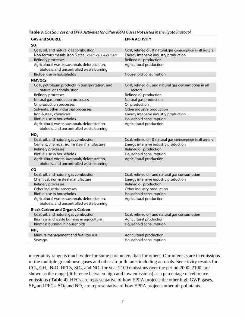
Table 3. Gas Sources and EPPA Activities for Other IGSM Gases Not Listed in the Kyoto Protocol

GAS and SOURCE EPPA ACTIVITY

SO2

Coal, oil, and natural gas combustion Coal, refined oil, & natural gas consumption in all sectors

Non-ferrous metals, iron & steel, chemicals, & cement Energy intensive industry productionRefinery processes Refined oil productionAgricultural waste, savannah, deforestation,

biofuels, and uncontrolled waste burningAgricultural production

Biofuel use in households Household consumption

NMVOCsCoal, petroleum products in transportation, and

natural gas combustionCoal, refined oil, and natural gas consumption in all

sectorsRefinery processes Refined oil productionNatural gas production processes Natural gas productionOil production processes Oil productionSolvents, other industrial processes Other industry productionIron & steel, chemicals Energy intensive industry productionBiofuel use in households Household consumptionAgricultural waste, savannah, deforestation,

biofuels, and uncontrolled waste burningAgricultural production

NOx

Coal, oil, and natural gas combustion Coal, refined oil, & natural gas consumption in all sectors

Cement, chemical, iron & steel manufacture Energy intensive industry productionRefinery processes Refined oil productionBiofuel use in households Household consumptionAgricultural waste, savannah, deforestation,

biofuels, and uncontrolled waste burningAgricultural production

COCoal, oil, and natural gas combustion Coal, refined oil, and natural gas consumptionChemical, iron & steel manufacture Energy intensive industry productionRefinery processes Refined oil productionOther industrial processes Other industry productionBiofuel use in households Household consumptionAgricultural waste, savannah, deforestation,

biofuels, and uncontrolled waste burningAgricultural production

Black Carbon and Organic CarbonCoal, oil, and natural gas combustion Coal, refined oil, and natural gas consumptionBiomass and waste burning in agriculture Agricultural productionBiomass burning in households Household consumption

NH3

Manure management and fertilizer use Agricultural productionSewage Household consumption

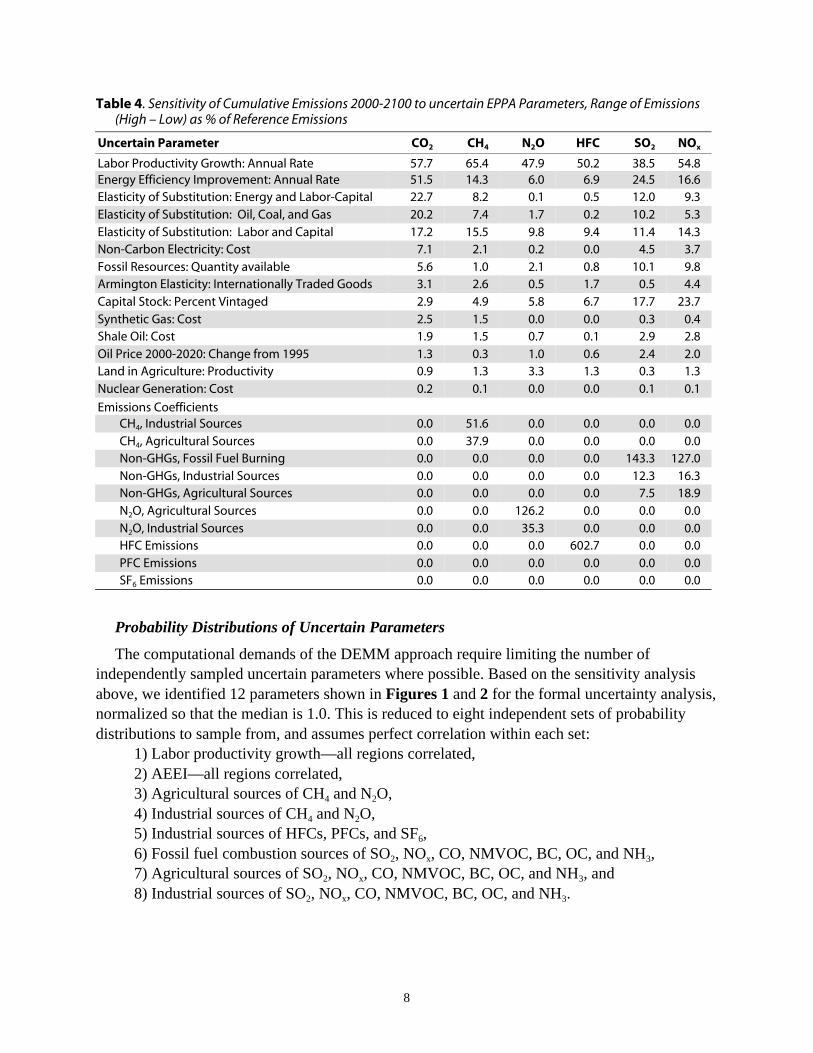
uncertainty range is much wider for some parameters than for others. Our interests are in emissionsof the multiple greenhouse gases and other air pollutants including aerosols. Sensitivity results forCO2, CH4, N2O, HFCs, SO2, and NOx for year 2100 emissions over the period 2000–2100, areshown as the range (difference between high and low emissions) as a percentage of referenceemissions (Table 4). HFCs are representative of how EPPA projects the other high GWP gases,SF6 and PFCs. SO2 and NOx are representative of how EPPA projects other air pollutants.

8

Table 4. Sensitivity of Cumulative Emissions 2000-2100 to uncertain EPPA Parameters, Range of Emissions(High – Low) as % of Reference Emissions

Uncertain Parameter CO2 CH4 N2O HFC SO2 NOx

Labor Productivity Growth: Annual Rate 57.7 65.4 47.9 50.2 38.5 54.8Energy Efficiency Improvement: Annual Rate 51.5 14.3 6.0 6.9 24.5 16.6Elasticity of Substitution: Energy and Labor-Capital 22.7 8.2 0.1 0.5 12.0 9.3Elasticity of Substitution: Oil, Coal, and Gas 20.2 7.4 1.7 0.2 10.2 5.3Elasticity of Substitution: Labor and Capital 17.2 15.5 9.8 9.4 11.4 14.3Non-Carbon Electricity: Cost 7.1 2.1 0.2 0.0 4.5 3.7Fossil Resources: Quantity available 5.6 1.0 2.1 0.8 10.1 9.8Armington Elasticity: Internationally Traded Goods 3.1 2.6 0.5 1.7 0.5 4.4Capital Stock: Percent Vintaged 2.9 4.9 5.8 6.7 17.7 23.7Synthetic Gas: Cost 2.5 1.5 0.0 0.0 0.3 0.4Shale Oil: Cost 1.9 1.5 0.7 0.1 2.9 2.8Oil Price 2000-2020: Change from 1995 1.3 0.3 1.0 0.6 2.4 2.0Land in Agriculture: Productivity 0.9 1.3 3.3 1.3 0.3 1.3Nuclear Generation: Cost 0.2 0.1 0.0 0.0 0.1 0.1

Emissions Coefficients CH4, Industrial Sources 0.0 51.6 0.0 0.0 0.0 0.0 CH4, Agricultural Sources 0.0 37.9 0.0 0.0 0.0 0.0 Non-GHGs, Fossil Fuel Burning 0.0 0.0 0.0 0.0 143.3 127.0 Non-GHGs, Industrial Sources 0.0 0.0 0.0 0.0 12.3 16.3 Non-GHGs, Agricultural Sources 0.0 0.0 0.0 0.0 7.5 18.9 N2O, Agricultural Sources 0.0 0.0 126.2 0.0 0.0 0.0 N2O, Industrial Sources 0.0 0.0 35.3 0.0 0.0 0.0 HFC Emissions 0.0 0.0 0.0 602.7 0.0 0.0 PFC Emissions 0.0 0.0 0.0 0.0 0.0 0.0 SF6 Emissions 0.0 0.0 0.0 0.0 0.0 0.0

Probability Distributions of Uncertain Parameters

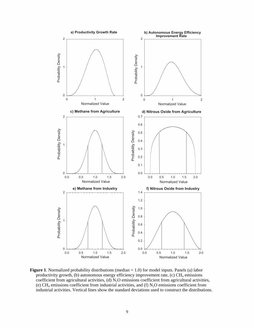
The computational demands of the DEMM approach require limiting the number ofindependently sampled uncertain parameters where possible. Based on the sensitivity analysisabove, we identified 12 parameters shown in Figures 1 and 2 for the formal uncertainty analysis,normalized so that the median is 1.0. This is reduced to eight independent sets of probabilitydistributions to sample from, and assumes perfect correlation within each set:

1) Labor productivity growth—all regions correlated,2) AEEI—all regions correlated,3) Agricultural sources of CH4 and N2O,4) Industrial sources of CH4 and N2O,5) Industrial sources of HFCs, PFCs, and SF6,6) Fossil fuel combustion sources of SO2, NOx, CO, NMVOC, BC, OC, and NH3,7) Agricultural sources of SO2, NOx, CO, NMVOC, BC, OC, and NH3, and8) Industrial sources of SO2, NOx, CO, NMVOC, BC, OC, and NH3.

9

c) Methane from Agriculture

Normalized Value

0.0 0.5 1.0 1.5 2.0

Pro

ba

bili

ty D

en

sity

0

1

2

d) Nitrous Oxide from Agriculture

Normalized Value

0.0 0.5 1.0 1.5 2.0

Pro

ba

bili

ty D

en

sity

0.0

0.1

0.2

0.3

0.4

0.5

0.6

0.7

f) Nitrous Oxide from Industry

Normalized Value

0.0 0.5 1.0 1.5 2.0

0.0

0.2

0.4

0.6

0.8

1.0

1.2

1.4e) Methane from Industry

Normalized Value

0.0 0.5 1.0 1.5 2.0

Pro

ba

bili

ty D

en

sity

Pro

ba

bili

ty D

en

sity

0

1

2

a) Productivity Growth Rate

Normalized Value

0 1 0 12 2

Pro

ba

bili

ty D

en

sity

0

1

2

b) Autonomous Energy Efficiency Improvement Rate

Normalized Value

Pro

ba

bili

ty D

en

sity

0

1

2

Figure 1. Normalized probability distributions (median = 1.0) for model inputs. Panels (a) laborproductivity growth, (b) autonomous energy efficiency improvement rate, (c) CH4 emissionscoefficient from agricultural activities, (d) N2O emissions coefficient from agricultural activities,(e) CH4 emissions coefficient from industrial activities, and (f) N2O emissions coefficient fromindustrial activities. Vertical lines show the standard deviations used to construct the distributions.

10

d) Non-GHGs - Fossil Fuel Combustion

Normalized Value

0.0 0.5 1.0 1.5 2.0

Pro

ba

bili

ty D

en

sity

0.0

0.1

0.2

0.3

0.4

0.5

0.6

0.7

a) Growth Rate for HFC Emissions

Normalized Value

0 1 2

Pro

ba

bili

ty D

en

sity

0

2

4

6

8

b) Growth Rate for PFC Emissions

Normalized Value

0 1 2 3 4 5

Pro

ba

bili

ty D

en

sity

0

1

2

3

4

c) Growth Rate for SF6 Emissions

Normalized Value

0 1 2

Pro

ba

bili

ty D

en

sity

0

2

4

6

8

10

12

e) Non-GHGs from Agriculture

Normalized Value

0.0 0.5 1.0 1.5 2.0 2.5 3.0

Pro

ba

bili

ty D

en

sity

0.0

0.1

0.2

0.3

0.4

0.5

0.6

f) Non-GHGs from Industry

Normalized Value

0.0 0.5 1.0 1.5 2.0

Pro

ba

bili

ty D

en

sity

0.0

0.2

0.4

0.6

0.8

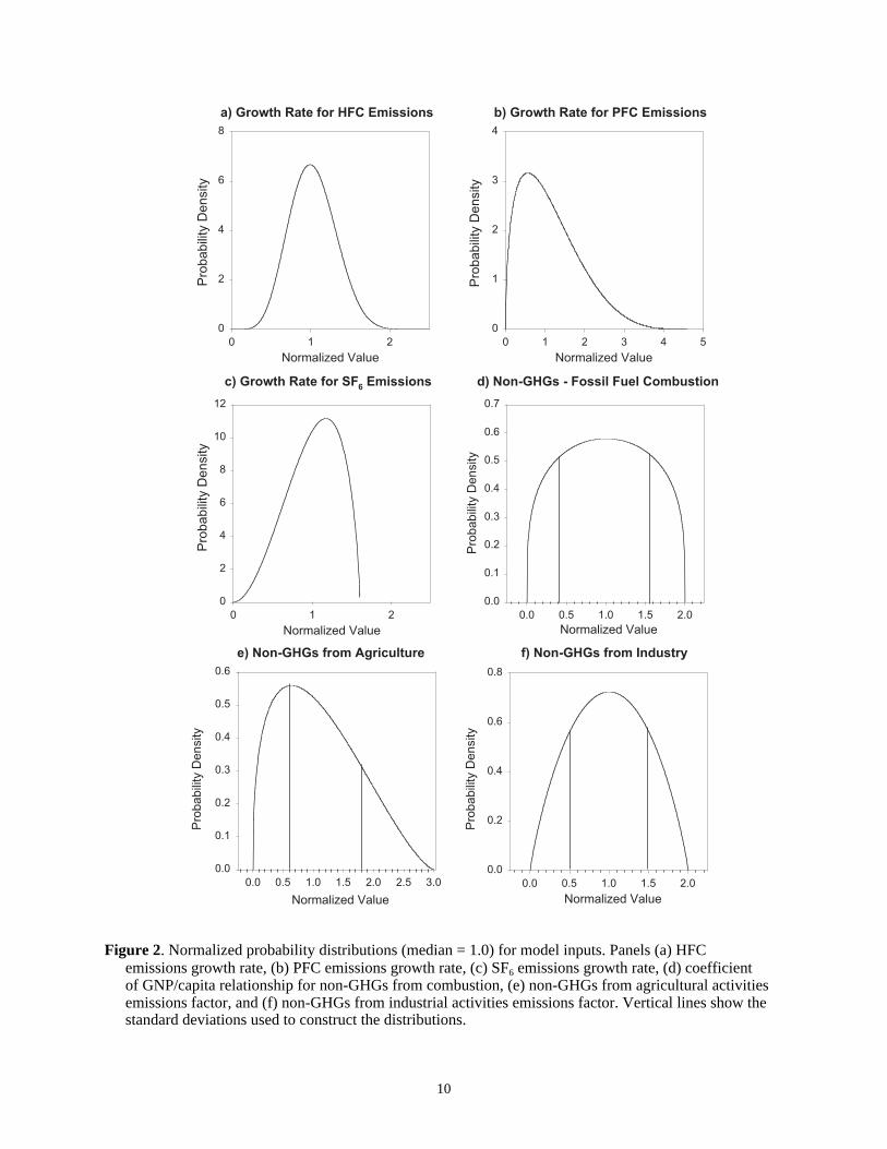
Figure 2. Normalized probability distributions (median = 1.0) for model inputs. Panels (a) HFCemissions growth rate, (b) PFC emissions growth rate, (c) SF6 emissions growth rate, (d) coefficientof GNP/capita relationship for non-GHGs from combustion, (e) non-GHGs from agricultural activitiesemissions factor, and (f) non-GHGs from industrial activities emissions factor. Vertical lines show thestandard deviations used to construct the distributions.

11

We constructed the distributions for uncertain parameters through expert elicitation and fromdata obtained from the literature. The probability distributions for labor productivity growth andAEEI were obtained by expert elicitation. Five economists5 participated in a protocol, eachproviding fractiles for the distribution for these variables. The five probability distributions foreach quantity were then combined by equally weighting each expert’s assessment. The experts’beliefs about the distribution of GDP growth rather than labor productivity were assessed as theexperts indicated greater familiarity with estimates of GDP growth. As modeled in EPPA, thereis a very close relationship between GDP growth (an output of EPPA) and the labor productivitygrowth required to produce that GDP growth, assuming all other parameters at reference values.Separate distributions for labor productivity growth were assessed for each of the EPPA regions,but in this uncertainty study we treat growth in all regions as perfectly correlated. Similarly,distributions for AEEI were elicited from the experts for OECD regions and separately for non-OECD regions, but treated as perfectly correlated during the random sampling.

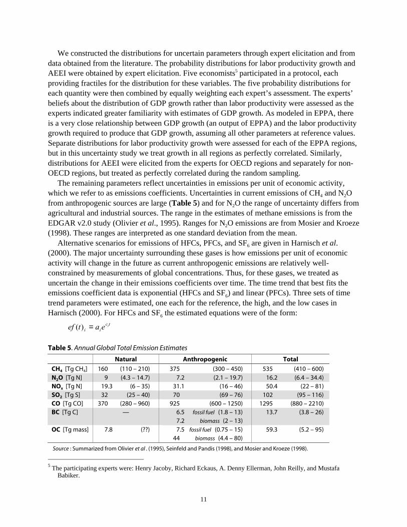
The remaining parameters reflect uncertainties in emissions per unit of economic activity,which we refer to as emissions coefficients. Uncertainties in current emissions of CH4 and N2Ofrom anthropogenic sources are large (Table 5) and for N2O the range of uncertainty differs fromagricultural and industrial sources. The range in the estimates of methane emissions is from theEDGAR v2.0 study (Olivier et al., 1995). Ranges for N2O emissions are from Mosier and Kroeze(1998). These ranges are interpreted as one standard deviation from the mean.

Alternative scenarios for emissions of HFCs, PFCs, and SF6 are given in Harnisch et al.(2000). The major uncertainty surrounding these gases is how emissions per unit of economicactivity will change in the future as current anthropogenic emissions are relatively well-constrained by measurements of global concentrations. Thus, for these gases, we treated asuncertain the change in their emissions coefficients over time. The time trend that best fits theemissions coefficient data is exponential (HFCs and SF6) and linear (PFCs). Three sets of timetrend parameters were estimated, one each for the reference, the high, and the low cases inHarnisch (2000). For HFCs and SF6 the estimated equations were of the form:

tcii

ieatef =)(

Table 5. Annual Global Total Emission Estimates

Natural Anthropogenic Total

CH4 [Tg CH4] 160 (110 – 210) 375 (300 – 450) 535 (410 – 600)N2O [Tg N] 9 (4.3 – 14.7) 7.2 (2.1 – 19.7) 16.2 (6.4 – 34.4)NOx [Tg N] 19.3 (6 – 35) 31.1 (16 – 46) 50.4 (22 – 81)SO2 [Tg S] 32 (25 – 40) 70 (69 – 76) 102 (95 – 116)CO [Tg CO] 370 (280 – 960) 925 (600 – 1250) 1295 (880 – 2210)BC [Tg C] — 6.5 fossil fuel (1.8 – 13)

7.2 biomass (2 – 13)13.7 (3.8 – 26)

OC [Tg mass] 7.8 (??) 7.5 fossil fuel (0.75 – 15)44 biomass (4.4 – 80)

59.3 (5.2 – 95)

Source : Summarized from Olivier et al . (1995), Seinfeld and Pandis (1998), and Mosier and Kroeze (1998).

5 The participating experts were: Henry Jacoby, Richard Eckaus, A. Denny Ellerman, John Reilly, and Mustafa

Babiker.

12

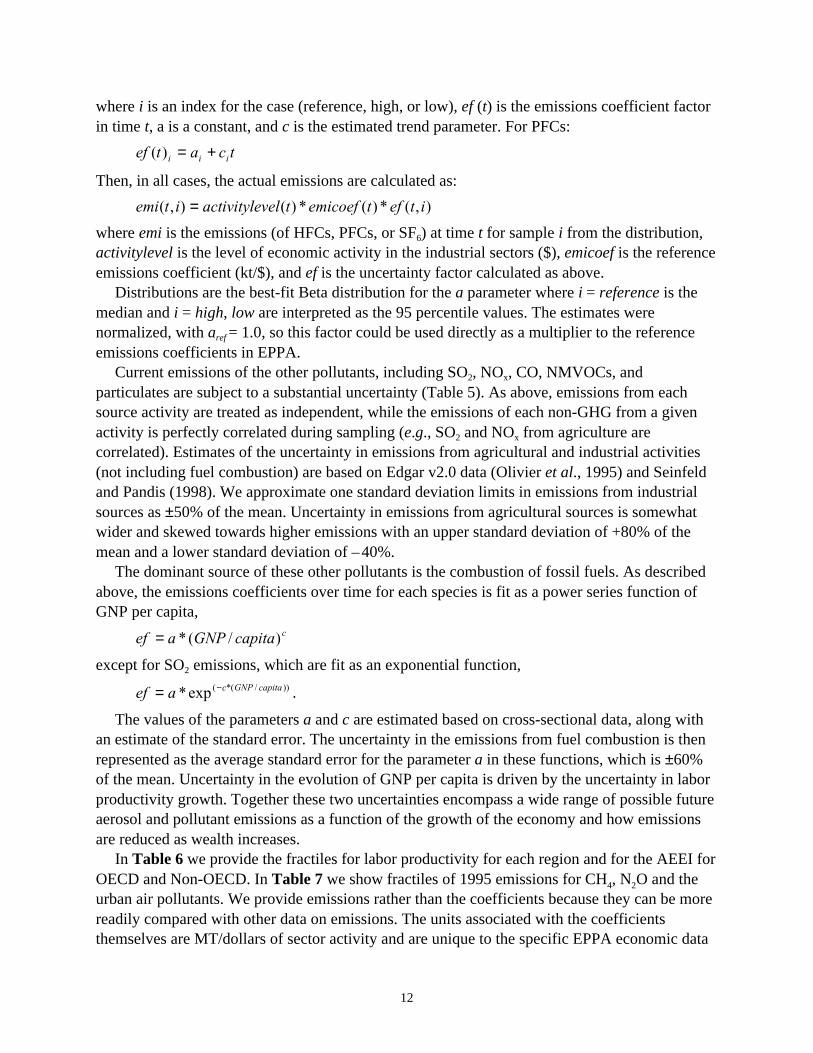
where i is an index for the case (reference, high, or low), ef (t) is the emissions coefficient factorin time t, a is a constant, and c is the estimated trend parameter. For PFCs:

tcatef iii +=)(

Then, in all cases, the actual emissions are calculated as:

),(*)(*)(),( iteftemicoeftvelactivityleitemi =

where emi is the emissions (of HFCs, PFCs, or SF6) at time t for sample i from the distribution,activitylevel is the level of economic activity in the industrial sectors ($), emicoef is the referenceemissions coefficient (kt/$), and ef is the uncertainty factor calculated as above.

Distributions are the best-fit Beta distribution for the a parameter where i = reference is themedian and i = high, low are interpreted as the 95 percentile values. The estimates werenormalized, with aref = 1.0, so this factor could be used directly as a multiplier to the referenceemissions coefficients in EPPA.

Current emissions of the other pollutants, including SO2, NOx, CO, NMVOCs, andparticulates are subject to a substantial uncertainty (Table 5). As above, emissions from eachsource activity are treated as independent, while the emissions of each non-GHG from a givenactivity is perfectly correlated during sampling (e.g., SO2 and NOx from agriculture arecorrelated). Estimates of the uncertainty in emissions from agricultural and industrial activities(not including fuel combustion) are based on Edgar v2.0 data (Olivier et al., 1995) and Seinfeldand Pandis (1998). We approximate one standard deviation limits in emissions from industrialsources as ±50% of the mean. Uncertainty in emissions from agricultural sources is somewhatwider and skewed towards higher emissions with an upper standard deviation of +80% of themean and a lower standard deviation of – 40%.

The dominant source of these other pollutants is the combustion of fossil fuels. As describedabove, the emissions coefficients over time for each species is fit as a power series function ofGNP per capita,

ccapitaGNPaef )/(*=

except for SO2 emissions, which are fit as an exponential function,))/(*(exp* capitaGNPcaef −= .

The values of the parameters a and c are estimated based on cross-sectional data, along withan estimate of the standard error. The uncertainty in the emissions from fuel combustion is thenrepresented as the average standard error for the parameter a in these functions, which is ±60%of the mean. Uncertainty in the evolution of GNP per capita is driven by the uncertainty in laborproductivity growth. Together these two uncertainties encompass a wide range of possible futureaerosol and pollutant emissions as a function of the growth of the economy and how emissionsare reduced as wealth increases.

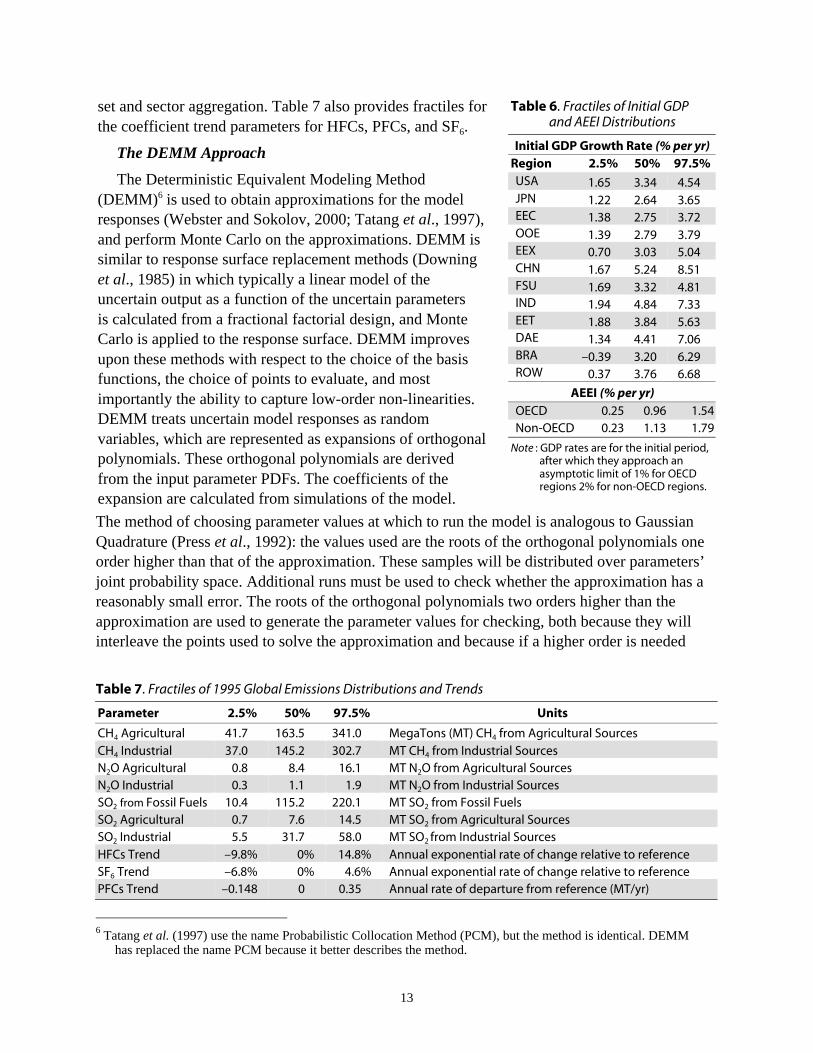
In Table 6 we provide the fractiles for labor productivity for each region and for the AEEI forOECD and Non-OECD. In Table 7 we show fractiles of 1995 emissions for CH4, N2O and theurban air pollutants. We provide emissions rather than the coefficients because they can be morereadily compared with other data on emissions. The units associated with the coefficientsthemselves are MT/dollars of sector activity and are unique to the specific EPPA economic data

13

Table 6. Fractiles of Initial GDPand AEEI Distributions

Initial GDP Growth Rate (% per yr)Region 2.5% 50% 97.5%USA 1.65 3.34 4.54JPN 1.22 2.64 3.65EEC 1.38 2.75 3.72OOE 1.39 2.79 3.79EEX 0.70 3.03 5.04CHN 1.67 5.24 8.51FSU 1.69 3.32 4.81IND 1.94 4.84 7.33EET 1.88 3.84 5.63DAE 1.34 4.41 7.06BRA –0.39 3.20 6.29ROW 0.37 3.76 6.68

AEEI (% per yr)OECD 0.25 0.96 1.54Non-OECD 0.23 1.13 1.79

Note : GDP rates are for the initial period,after which they approach anasymptotic limit of 1% for OECDregions 2% for non-OECD regions.

set and sector aggregation. Table 7 also provides fractiles forthe coefficient trend parameters for HFCs, PFCs, and SF6.

The DEMM Approach

The Deterministic Equivalent Modeling Method(DEMM)6 is used to obtain approximations for the modelresponses (Webster and Sokolov, 2000; Tatang et al., 1997),and perform Monte Carlo on the approximations. DEMM issimilar to response surface replacement methods (Downinget al., 1985) in which typically a linear model of theuncertain output as a function of the uncertain parametersis calculated from a fractional factorial design, and MonteCarlo is applied to the response surface. DEMM improvesupon these methods with respect to the choice of the basisfunctions, the choice of points to evaluate, and mostimportantly the ability to capture low-order non-linearities.DEMM treats uncertain model responses as randomvariables, which are represented as expansions of orthogonalpolynomials. These orthogonal polynomials are derivedfrom the input parameter PDFs. The coefficients of theexpansion are calculated from simulations of the model.

The method of choosing parameter values at which to run the model is analogous to GaussianQuadrature (Press et al., 1992): the values used are the roots of the orthogonal polynomials oneorder higher than that of the approximation. These samples will be distributed over parameters’joint probability space. Additional runs must be used to check whether the approximation has areasonably small error. The roots of the orthogonal polynomials two orders higher than theapproximation are used to generate the parameter values for checking, both because they willinterleave the points used to solve the approximation and because if a higher order is needed

Table 7. Fractiles of 1995 Global Emissions Distributions and Trends

Parameter 2.5% 50% 97.5% Units

CH4 Agricultural 41.7 163.5 341.0 MegaTons (MT) CH4 from Agricultural SourcesCH4 Industrial 37.0 145.2 302.7 MT CH4 from Industrial SourcesN2O Agricultural 0.8 8.4 16.1 MT N2O from Agricultural SourcesN2O Industrial 0.3 1.1 1.9 MT N2O from Industrial SourcesSO2 from Fossil Fuels 10.4 115.2 220.1 MT SO2 from Fossil FuelsSO2 Agricultural 0.7 7.6 14.5 MT SO2 from Agricultural SourcesSO2 Industrial 5.5 31.7 58.0 MT SO2 from Industrial SourcesHFCs Trend –9.8% 0% 14.8% Annual exponential rate of change relative to referenceSF6 Trend –6.8% 0% 4.6% Annual exponential rate of change relative to referencePFCs Trend –0.148 0 0.35 Annual rate of departure from reference (MT/yr)

6 Tatang et al. (1997) use the name Probabilistic Collocation Method (PCM), but the method is identical. DEMM

has replaced the name PCM because it better describes the method.

14

these runs are immediately available. DEMM typically converges on estimates of the mean,variance, and extreme fractiles of multiple responses by second or third order expansions (for2 parameters, 3rd order requires 10 simulations to solve the approximation, plus several more toassess the accuracy) whereas other methods such as Latin Hypercube sampling (LHS) (McKayet al., 1979) requires more runs to accurately represent higher order moments.

The approximation of model responses by DEMM has additional advantages. Information onthe sensitivity to individual parameters is accurately represented in the expansion, allowing theevaluation of relative contribution to uncertainty without additional simulations. Finally,alternative PDFs for parameters can be propagated through the approximation without anyadditional runs of the true model, as long as the new PDFs do not extend beyond the range forwhich the approximation has been validated. LHS and other methods would require new sets ofsimulations at additional computational cost.

1.2 Emissions Uncertainty Results

Using DEMM, we propagate the uncertainty in 8 independent sets of input parameters byestimating 4th order polynomial expansions, requiring 1300 runs of EPPA for estimation andverification. The errors in the reduced form model were all less than 0.1% of the mean values,and most are less than 0.01% of the mean. Monte Carlo simulation is then performed on thereduced form model using 10,000 random samples from the parameter distributions. Theresulting samples of emissions of each species at each time period are then used to constructprobability distributions.

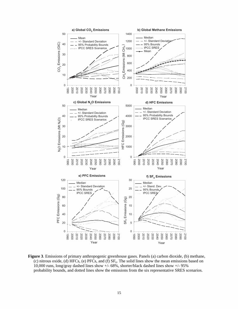
The resulting uncertainty in greenhouse gas emissions is shown in Figure 3, which indicatethe median, +/- one standard deviation (67%), and +/- two standard deviations (95%) for theemissions of each gas. Also shown in Figure 3 are the emissions from the six representativescenarios from the IPCC SRES. Although the SRES scenarios do not have an associatedprobability, it is useful to compare them to our probabilistic bounds. CO2 emissions from theSRES scenarios spread over much of our 95% range (Figure 3a). This is not surprising, sincesocioeconomic models of many types have been used to project CO2 emissions for nearly twodecades, and modeling studies tend to be fairly consistent (Weyant and Hill, 1999). But while therange itself is similar, the distributions are not. The SRES has a lower bias among its scenarios,with four of the six SRES scenarios well below our median emissions in 2100. Furthermore, twoof those project lower CO2 emissions by 2100 than our 95% lower bound. The time path ofemissions is even less consistent between the two methods; the SRES scenarios are biased higherthan our distributions before 2040, after which time some of the SRES change the trend.

Emissions projections of other greenhouse gases are less consistent between our ranges andthe IPCC’s. One significant difference is that the IPCC assumes that global emissions of all gasesare known for 1990–2000. In fact, as discussed in the previous section, there is considerableuncertainty in current global emissions, particularly emissions resulting from agriculturalactivities and emissions from developing countries. Perhaps as a result of our treatment ofcurrent uncertainty as well as future trends, we find a larger range of uncertainty in non-CO2

greenhouse gas emissions than the IPCC does. SRES projections of CH4 and N2O span our 67%probability bounds. Four of the six N2O scenarios are near the lower 67% bound while the othertwo are near the upper 67% bound, and none are close to our mean.

15

a) Global CO2 Emissions

Year

19

90

20

00

20

10

20

20

20

30

20

40

20

50

20

60

20

70

20

80

20

90

21

00

CO

2 E

mis

sio

ns (

GtC

)

0

10

20

30

40

50

Mean

+/- Standard Deviation

95% Probability Bounds

IPCC SRES Scenarios

b) Global Methane Emissions

Year

20

00

20

10

20

20

20

30

20

40

20

50

20

60

20

70

20

80

20

90

21

00

CH

44 E

mis

sio

ns (

Mt C

H)

0

200

400

600

800

1000

1200

1400

Median

+/- Standard Deviation

95% Bounds

IPCC SRES

Mean

c) Global N2O Emissions

Year1

99

0

20

00

20

10

20

20

20

30

20

40

20

50

20

60

20

70

20

80

20

90

21

00

2N

O E

mis

sio

ns (

Mt N

O)

0

10

20

30

40

50

Median

+/- Standard Deviation

95% Probability Bounds

IPCC SRES Scenarios

d) HFC Emissions

Year

19

90

20

00

20

10

20

20

20

30

20

40

20

50

20

60

20

70

20

80

20

90

21

00

HF

C E

mis

sio

ns (

Gg

)

0

1000

2000

3000

4000

5000Median

+/- Standard Deviation

95% Probability Bounds

IPCC SRES Scenarios

e) PFC Emissions

Year

19

90

20

00

20

10

20

20

20

30

20

40

20

50

20

60

20

70

20

80

20

90

21

00

PF

C E

mis

sio

ns (

Gg

)

0

20

40

60

80

100

120Median

+/- Standard Deviation

95% Bounds

IPCC SRES

f) SF6 Emissions

Year

19

90

20

00

20

10

20

20

20

30

20

40

20

50

20

60

20

70

20

80

20

90

21

00

6 S

F

Em

issio

ns (

Gg

)

0

5

10

15

20

25

30Median

+/- Stand. Dev.

95% Bounds

IPCC SRES

2

Figure 3. Emissions of primary anthropogenic greenhouse gases. Panels (a) carbon dioxide, (b) methane,(c) nitrous oxide, (d) HFCs, (e) PFCs, and (f) SF6. The solid lines show the mean emissions based on10,000 runs, long/gray dashed lines show +/- 68%, shorter/black dashed lines show +/- 95%probability bounds, and dotted lines show the emissions from the six representative SRES scenarios.

16

For the F-gases (hydrofluorocarbons, perfluorocarbons, and sulfur hexafluoride) the IPCC hasdeveloped four representative scenarios (Fenhann, 2000; SRES, 2000). Their projections ofHFCs emissions span considerably less than our 67% probability range. The higher HFCsemission trajectories in EPPA permit strong increases of emission levels as a consequence ofincreases of GDP. In contrast, the SRES emissions remain capped because of a prescribed de-coupling of HFCs from increases of GDP due to market saturation. The low HFCs emissionlevels, which are also possible within EPPA, are also not seen in SRES, as its authors seem fairlypessimistic about the potential for emission control through containment and substitution byalternative fluids. For PFCs the authors of SRES seem skeptical about the availability oftechnological options to reduce PFCs emissions from aluminum production eventually leading toPFCs free production. The picture is similar for SF6: SRES again does not allow for a permanentde-coupling of emissions from economic development, which in EPPA becomes possiblethrough technological change. All in all, SRES—with respect to emissions of fluorinatedgases—assumes a fairly deterministic emission-GDP relation that does not allow for majortechnological changes to lead to truly significant reductions of emissions.

Global SO2 Emissions

Year

19

90

20

00

20

10

20

20

20

30

20

40

20

50

20

60

20

70

20

80

20

90

21

00

Em

issio

ns (

Mt S

O2)

0

100

200

300

400

500Mean

68% Probability Bounds

95% Probability Bounds

IPCC SRES Scenarios

Global NOx Emissions

Year

19

90

20

00

20

10

20

20

20

30

20

40

20

50

20

60

20

70

20

80

20

90

21

00

Em

issio

ns (

Mt N

O

x )

0

200

400

600

800

1000

1200

Mean

68% Probability Bounds

95% Probability Bounds

IPCC SRES Scenarios

CO Emissions

Year

19

90

20

00

20

10

20

20

20

30

20

40

20

50

20

60

20

70

20

80

20

90

21

00

CO

Em

issio

ns (

Mt C

O)

0

1000

2000

3000

4000

5000

6000Median

68% Probability Bounds

95% Probability Bounds

IPCC SRES Scenarios

VOC Emissions

Year

19

90

20

00

20

10

20

20

20

30

20

40

20

50

20

60

20

70

20

80

20

90

21

00

VO

C E

mis

sio

ns (

Mt)

0

200

400

600

800

1000

1200Median

68% Probability Bounds

95% Probability Bounds

IPCC SRES Scenarios

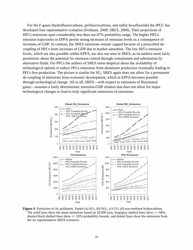
Figure 4. Emissions of air pollutants. Panels (a) SO2, (b) NOx, (c) CO, (d) non-methane hydrocarbons.The solid lines show the mean emissions based on 10,000 runs, long/gray dashed lines show +/- 68%,shorter/black dashed lines show +/- 95% probability bounds, and dotted lines show the emissions fromthe six representative SRES scenarios.

17

In addition to the greenhouse gas emissions, we use the 10,000 simulations to quantifyuncertainty in other climatically relevant emissions. In Figure 4, we show the uncertainty inemissions of SO2, NOx, CO, and non-methane hydrocarbons. As with the greenhouse gases, ourprobability bounds account for uncertainty in current global emissions of these species as well aseconomic growth, while the IPCC assumes that current emissions are known. SO2 emissions, aprecursor to sulfate aerosols, are especially important in climate projections because of the strongnegative radiative forcing effect of those aerosols. The difference between the SRES projectionsof SO2 emissions to our projections is striking. In all six of the representative scenarios, the IPCCprojects that after about 2040, SO2 emissions will begin to steadily decline. The IPCC assumesthat policies will be implemented to reduce sulfur emissions, even in developing countries, in allimaginable cases. By contrast, our study imagines that the ability or willingness to implementsulfur emissions reduction policies is one of the key uncertainties in these projections.Accordingly, our 95% probability range includes the possibility of continuing increases in SO2

emissions over the next century, as well as declining emissions consistent with SRES. Similarly,though not as striking, SRES projections of NOx, CO, and NMVOC emissions all fall within thelower half of our probability distributions of emissions.

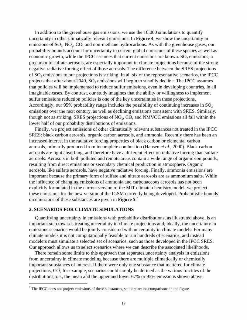
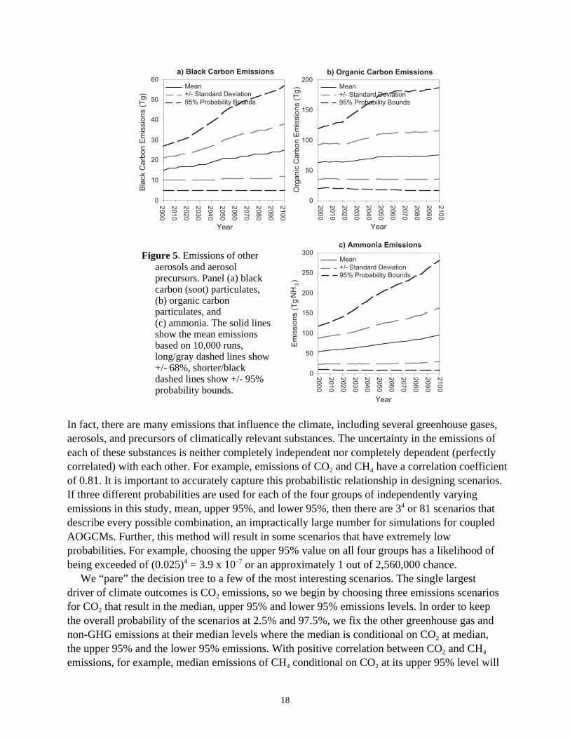
Finally, we project emissions of other climatically relevant substances not treated in the IPCCSRES: black carbon aerosols, organic carbon aerosols, and ammonia. Recently there has been anincreased interest in the radiative forcing properties of black carbon or elemental carbonaerosols, primarily produced from incomplete combustion (Hansen et al., 2000). Black carbonaerosols are light absorbing, and therefore have a different effect on radiative forcing than sulfateaerosols. Aerosols in both polluted and remote areas contain a wide range of organic compounds,resulting from direct emissions or secondary chemical production in atmosphere. Organicaerosols, like sulfate aerosols, have negative radiative forcing. Finally, ammonia emissions areimportant because the primary form of sulfate and nitrate aerosols are as ammonium salts. Whilethe influence of changing emissions of ammonia and carbonaceous aerosols has not beenexplicitly formulated in the current version of the MIT climate-chemistry model, we projectthese emissions for the new version of the IGSM currently being developed. Probabilistic boundson emissions of these substances are given in Figure 5.7

2. SCENARIOS FOR CLIMATE SIMULATIONS

Quantifying uncertainty in emissions with probability distributions, as illustrated above, is animportant step towards treating uncertainty in climate projections and, ideally, the uncertainty inemissions scenarios would be jointly considered with uncertainty in climate models. For manyclimate models it is not computationally feasible to run hundreds of scenarios, and insteadmodelers must simulate a selected set of scenarios, such as those developed in the IPCC SRES.Our approach allows us to select scenarios where we can describe the associated likelihoods.

There remain some limits to this approach that separates uncertainty analysis in emissionsfrom uncertainty in climate modeling because there are multiple climatically or chemicallyimportant substances of interest. If there were only one substance that mattered for climateprojections, CO2 for example, scenarios could simply be defined as the various fractiles of thedistributions; i.e., the mean and the upper and lower 67% or 95% emissions shown above. 7 The IPCC does not project emissions of these substances, so there are no comparisons in the figure.

18

a) Black Carbon Emissions

Year

20

00

20

10

20

20

20

30

20

40

20

50

20

60

20

70

20

80

20

90

21

00

Bla

ck C

arb

on

Em

issio

ns (

Tg

)

0

10

20

30

40

50

60Mean

+/- Standard Deviation

95% Probability Bounds

b) Organic Carbon Emissions

Year

20

00

20

10

20

20

20

30

20

40

20

50

20

60

20

70

20

80

20

90

21

00

Org

an

ic C

arb

on

Em

issio

ns (

Tg

)

0

50

100

150

200Mean

+/- Standard Deviation

95% Probability Bounds

Figure 5. Emissions of otheraerosols and aerosolprecursors. Panel (a) blackcarbon (soot) particulates,(b) organic carbonparticulates, and(c) ammonia. The solid linesshow the mean emissionsbased on 10,000 runs,long/gray dashed lines show+/- 68%, shorter/blackdashed lines show +/- 95%probability bounds.

c) Ammonia Emissions

Year

20

00

20

10

20

20

20

30

20

40

20

50

20

60

20

70

20

80

20

90

21

00

NH

3 E

mis

sio

ns (

Tg

)

0

50

100

150

200

250

300Mean

+/- Standard Deviation

95% Probability Bounds

In fact, there are many emissions that influence the climate, including several greenhouse gases,aerosols, and precursors of climatically relevant substances. The uncertainty in the emissions ofeach of these substances is neither completely independent nor completely dependent (perfectlycorrelated) with each other. For example, emissions of CO2 and CH4 have a correlation coefficientof 0.81. It is important to accurately capture this probabilistic relationship in designing scenarios.If three different probabilities are used for each of the four groups of independently varyingemissions in this study, mean, upper 95%, and lower 95%, then there are 34 or 81 scenarios thatdescribe every possible combination, an impractically large number for simulations for coupledAOGCMs. Further, this method will result in some scenarios that have extremely lowprobabilities. For example, choosing the upper 95% value on all four groups has a likelihood ofbeing exceeded of (0.025)4 = 3.9 x 10–7 or an approximately 1 out of 2,560,000 chance.

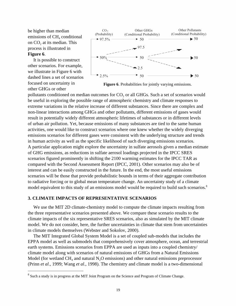
We “pare” the decision tree to a few of the most interesting scenarios. The single largestdriver of climate outcomes is CO2 emissions, so we begin by choosing three emissions scenariosfor CO2 that result in the median, upper 95% and lower 95% emissions levels. In order to keepthe overall probability of the scenarios at 2.5% and 97.5%, we fix the other greenhouse gas andnon-GHG emissions at their median levels where the median is conditional on CO2 at median,the upper 95% and the lower 95% emissions. With positive correlation between CO2 and CH4

emissions, for example, median emissions of CH4 conditional on CO2 at its upper 95% level will

19

be higher than medianemissions of CH4 conditionalon CO2 at its median. Thisprocess is illustrated inFigure 6.

It is possible to constructother scenarios. For example,we illustrate in Figure 6 withdashed lines a set of scenariosfocused on uncertainty inother GHGs or other

CO 2

(Probability) Other GHGs

(Conditional Probability) Other Pollutants

(Conditional Probability)

97.5% 50 50 97.5

50% 50 50 2.5

2.5% 50 50

Figure 6. Probabilities for jointly varying emissions.

pollutants conditioned on median outcomes for CO2 or all GHGs. Such a set of scenarios wouldbe useful in exploring the possible range of atmospheric chemistry and climate responses toextreme variations in the relative increase of different substances. Since there are complex andnon-linear interactions among GHGs and other pollutants, different emissions of gases wouldresult in potentially widely different atmospheric lifetimes of substances or in different levelsof urban air pollution. Yet, because emissions of many substances are tied to the same humanactivities, one would like to construct scenarios where one knew whether the widely divergingemissions scenarios for different gases were consistent with the underlying structure and trendsin human activity as well as the specific likelihood of such diverging emissions scenarios.A particular application might explore the uncertainty in sulfate aerosols given a median estimateof GHG emissions, as reductions in sulfate aerosol loadings projected in the IPCC SRESscenarios figured prominently in shifting the 2100 warming estimates for the IPCC TAR ascompared with the Second Assessment Report (IPCC, 2001). Other scenarios may also be ofinterest and can be easily constructed in the future. In the end, the most useful emissionsscenarios will be those that provide probabilistic bounds in terms of their aggregate contributionto radiative forcing or to global mean temperature change. An uncertainty study of a climatemodel equivalent to this study of an emissions model would be required to build such scenarios.8

3. CLIMATE IMPACTS OF REPRESENTATIVE SCENARIOS

We use the MIT 2D climate-chemistry model to compute the climate impacts resulting fromthe three representative scenarios presented above. We compare these scenario results to theclimate impacts of the six representative SRES scenarios, also as simulated by the MIT climatemodel. We do not consider, here, the further uncertainties in climate that stem from uncertaintiesin climate models themselves (Webster and Sokolov, 2000).

The MIT Integrated Global System Model is a set of coupled sub-models that includes theEPPA model as well as submodels that comprehensively cover atmosphere, ocean, and terrestrialearth systems. Emissions scenarios from EPPA are used as inputs into a coupled chemistry/climate model along with scenarios of natural emissions of GHGs from a Natural EmissionsModel (for wetland CH4 and natural N2O emissions) and other natural emissions preprocessor(Prinn et al., 1999; Wang et al., 1998). The chemistry and climate model is a two-dimensional

8 Such a study is in progress at the MIT Joint Program on the Science and Program of Climate Change.

20

(2D) land-ocean (LO) resolving climate model, which is coupled to a 2D model of atmosphericchemistry and a 2D or three-dimensional (3D) model of ocean circulations (Sokolov and Stone,1998; Wang et al., 1998; Wang and Prinn, 1999). In addition to the 2D global chemistry, theIGSM includes a 3D urban air chemistry model for treating emissions in urban areas (Mayer etal., 2000). The TEM model of the Marine Biological Laboratory (Melillo et al., 1993; Tian et al.,1999; Xiao et al., 1997, 1998) simulates carbon and nitrogen dynamics of terrestrial ecosystems.These features allow the IGSM to project concentrations of the relevant trace gases, accountingfor photochemical processes and the feedback of climate on natural emission sources; radiativeforcing from these trace gases; temperature and precipitation at different latitudes (longitudinallyaveraged) and global mean; and sea level rise due to thermal expansion of the oceans.

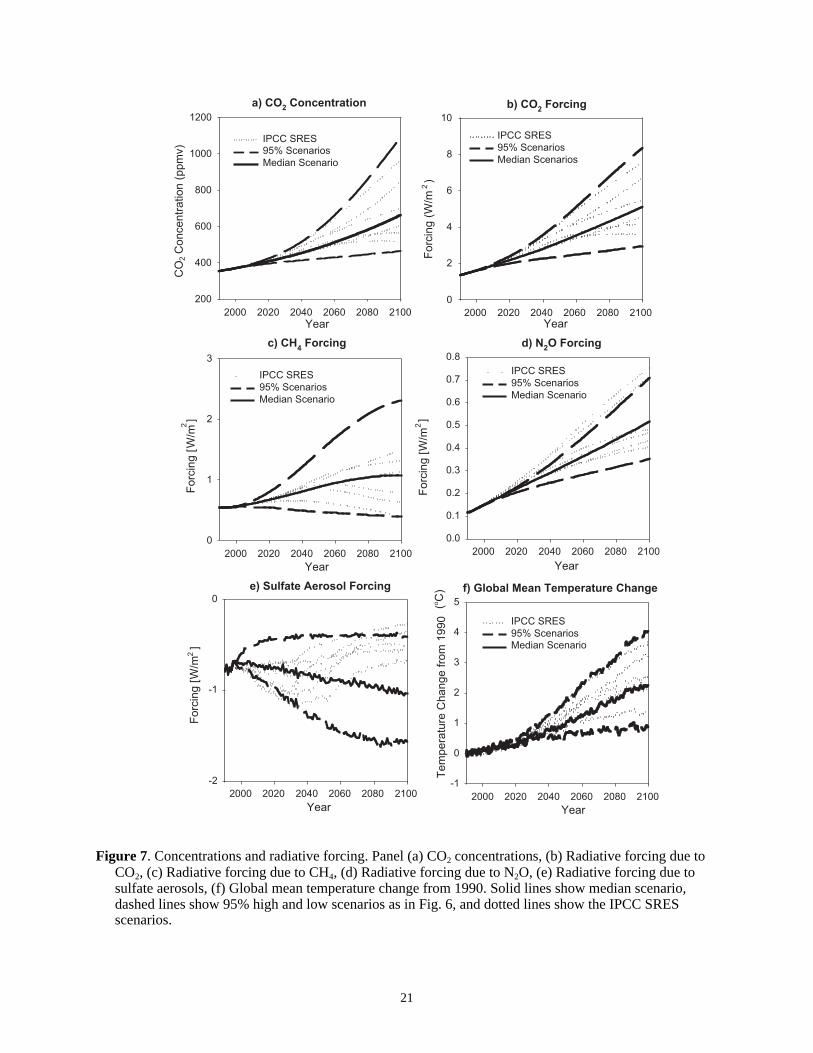
We find that the CO2 concentration by 2100 reaches 465 ppm, 662 ppm, and 1090 ppm in thelow, median, and high scenarios, respectively (Figure 7a). The SRES span a similar range, from518 ppm to 965 ppm because of the comparable ranges in CO2 emissions. Radiative forcing dueto CO2 alone in our scenarios ranges from 3.0 to 8.4 W/m2 by 2100, and the SRES scenariosresult in a similar range. In contrast, the ranges of radiative forcing resulting from otherradiatively active substances exhibit greater differences between our scenarios and the SRES.For methane forcing, our scenarios range from 0.4 to 2.3 W/m2 by 2100, while the SRES coversa smaller range and is biased towards lower forcings, from 1.1 to only 1.3 W/m2. Recall thatalthough parameters that drive both CO2 and CH4 are at extreme values in the high and lowcases, other uncertainties specific to CH4 are at median values; our range is not as large as a full95% confidence interval for CH4 forcing would be. Radiative forcing from N2O in the SREScovers a more similar range to that of our scenarios, but the SRES are biased towards higherforcings in this case. The combined radiative forcing effects of HFCs, PFCs, SF6, and CFCs arealso biased higher in the SRES. Our three scenarios have radiative forcings of 0.2, 0.5, and 0.9W/m2, while the SRES scenarios range from 0.4 to 0.9 W/m2.

Perhaps the most important differences are the sulfate aerosol contributions to radiativeforcing in our analysis compared with the SRES scenarios. The sulfate forcing in our scenarios is–0.4, –1.0, and –1.6 W/m2 by 2100 in the low, median, and high scenarios, respectively. Bycontrast, the range of forcings from the SRES scenarios is –0.3 to –0.7 W/m2. Our wider rangestems from two factors: (1) we represent uncertainty in existing sulfate loading, recognizing thatSO2 emissions come from many sources (e.g., energy and biomass burning and industrialprocesses) that are not all monitored and measured with great accuracy; and (2) we relatereductions in emissions of SO2 per unit of fuel combustion and other sources to growth in percapita income to reflect the growing demand for environmental clean-up with rising incomes thathas been observed. As a result of (1), once the wide uncertainty range for emissions in 2000 isrepresented in the climate chemistry IGSM there is an immediate response, representinguncertainty in current levels of radiative forcing. As a result of (2) and other assumptions aboutthe trend in emissions coefficients, we find the possibility of either increasing or decreasingsulfate aerosol forcing. The SRES scenarios include no uncertainty in current emissions of SO2

and all scenarios show radiative forcing in 2100 to be below current levels of forcing. There areother ways to represent uncertainty in future SO2 emissions that could change our results but,apart from any modeling, an adequate representation of uncertainty would seem to involve somemeasurable chance that SO2 emissions might increase rather than decrease. Figure 7(f) shows theresulting global mean temperature change from 1990 as a result of our three scenarios and the sixrepresentative SRES scenarios.

21

a) CO2 Concentration

Year2000 2020 2040 2060 2080 2100

CO

2 C

on

ce

ntr

atio

n (

pp

mv)

200

400

600

800

1000

1200

IPCC SRES

95% Scenarios

Median Scenario

b) CO2 Forcing

Year2000 2020 2040 2060 2080 2100

Fo

rcin

g (

W/m

2)

0

2

4

6

8

10

IPCC SRES

95% Scenarios

Median Scenarios

c) CH4 Forcing

Year

2000 2020 2040 2060 2080 2100

Fo

rcin

g [

W/m

2]

0

1

2

3

IPCC SRES

95% Scenarios

Median Scenario

IPCC SRES

95% Scenarios

Median Scenario

d) N2O Forcing

Year

2000 2020 2040 2060 2080 2100

Fo

rcin

g [

W/m

2]

0.0

0.1

0.2

0.3

0.4

0.5

0.6

0.7

0.8

e) Sulfate Aerosol Forcing

Year

2000 2020 2040 2060 2080 2100

Fo

rcin

g [

W/m

]

-2

-1

0f) Global Mean Temperature Change

Year

2000 2020 2040 2060 2080 2100

Te

mp

era

ture

Ch

an

ge

fro

m 1

99

0

(oC

)

-1

0

1

2

3

4

5

IPCC SRES

95% Scenarios

Median Scenario

2

Figure 7. Concentrations and radiative forcing. Panel (a) CO2 concentrations, (b) Radiative forcing due toCO2, (c) Radiative forcing due to CH4, (d) Radiative forcing due to N2O, (e) Radiative forcing due tosulfate aerosols, (f) Global mean temperature change from 1990. Solid lines show median scenario,dashed lines show 95% high and low scenarios as in Fig. 6, and dotted lines show the IPCC SRESscenarios.

22

Because CO2 is the largest single driver, the ranges of temperature changes are not extremelydifferent: our scenarios range from 0.9 to 4.0 oC, and the SRES range from 1.3 to 3.6 oC.However, it is interesting to note that the temperature change in five of the six SRES scenarios isgreater than or equal to the temperature change in our median scenario of 2.2 oC. The mainreason for the difference in the median or central tendency of the two sets of scenarios is thedifference in sulfate aerosol forcing. It is important to be clear that the range of global meantemperature change between our low and high scenarios is not a 95% confidence bound ontemperature change from the MIT model. To give this range will require applying the methodsdescribed here to a full uncertainty analysis of the climate model.

4. CONCLUSIONS

Analysis of possible future climate changes should include quantification of the uncertainty inclimate projections. In this paper, we constructed three representative scenarios where theemissions of CO2 are at median, upper 95%, and lower 95% levels, and all other emissions are attheir median levels conditional on the CO2 emissions. We have compared emissions from the sixrepresentative SRES scenarios with our calculated probability distributions of emissions, and alsocompare the climate impacts of the SRES scenarios with the impacts from our low, median, andhigh CO2 scenarios. We find that the SRES CO2 emissions covers much of our 95% confidencerange, but is biased towards lower CO2 emissions by the end of the century than our distributions.The differences partly reflect the inclusion of policy effects in some of the SRES scenarios,whereas we have tried to develop probability distributions of emissions under no climate policy.Assessments of the effects of policy would require repeating this exercise under the policyassumption, and then comparing the resulting probability distributions and their impacts.

For other greenhouse gases and aerosols, the SRES scenarios tend to encompass muchnarrower ranges than we find from uncertainty propagation. Further, the SRES emissions arebiased higher than our distributions for some species and biased lower for others. One differenceis that the IPCC does not include the uncertainty in current emission levels, which is significantin many cases. Finally, the greatest difference between the two methods is found in sulfuremissions. Here, the IPCC has assumed the presence of sulfate reduction policies later in thecentury seemingly without considering uncertainty in the ability/willingness to implement suchpolicies. In performing the uncertainty analysis, we also include the effect sulfate reductions aseconomies increase in wealth, but we have also included the uncertainty in how that relationshipwill hold in other countries in the future.

As a result of the different methods and assumptions in constructing representative scenarios,we find that the IPCC SRES are biased in the direction of higher global mean temperaturechange by the end of the next century. This bias towards higher temperatures is partly due to thestrongly optimistic assumptions about the reductions in sulfur emissions.

A significant motivation for this study was the perceived desire within the climate modelingcommunity for a small set of scenarios that describe a central tendency (mean or median) andhigh and low cases that bound an explicit probability. We hope these emissions scenariosprovide a useful set of scenarios to study climate uncertainties.

23

AcknowledgmentsOur thanks to our colleagues in the Joint Program for crucial contributions to this paper and tothe development of the IGSM model. Particular thanks to Chris Forest, Andrei Sokolov, RichardEckaus, David Reiner, Henry Jacoby, and Denny Ellerman. The IGSM has been developed aspart of the Joint Program on the Science and Policy of Global Change with the support of agovernment-industry partnership including the US Department of Energy (901214-HAR; DE-FG02-94ER61937; DE-FG0293ER61713) and a group of corporate sponsors from the UnitedStates and other countries. Research on other gases was conducted with funding support from theUS Environmental Protection Agency (X-827703-01-0).

REFERENCES

Babiker, M., Reilly, J. and Jacoby, H. (2000). The Kyoto Protocol and Developing Countries.Energy Policy 28: 525-536.

Babiker, M., Reilly, J., Mayer, M., Eckaus, R., Sue Wing, I. and Hyman, R. (2001). The MITEmissions Prediction and Policy Analysis Model: Revisions, Sensitivities, and Comparisonsof Results. MIT Joint Program on the Science and Policy of Global Change Report No. 71,Cambridge, MA.

Edmonds, J. and Reilly, J. (1985). Global Energy: Assessing the Future. Oxford UniversityPress: 317 p.

Downing, D.J., Gardner, R.H. and Hoffman, F.O. (1985). Response Surface Methodologies forUncertainty Analysis in Assessment Models. Technometrics 27(2): 151-163.

Fenhann, J. (2000). HFC, PFC and SF6 Emission Scenarios: Recent Development in IPCCSpecial Report on Emission Scenarios. In: Non-CO2 Greenhouse Gases: Scientificunderstanding, control and implementation: Proceedings of the Second InternationalSymposium on Non-CO2 Greenhouse Gases, van Ham, J., Baede, A.P.M., Meyer, L.A. andYbema, R. (eds.). Kluwer Academic Publishers, Dordrecht, Netherlands.

Harnisch, J., Jacoby, H.D., Prinn, R.G., and Wang, C. (2000). Regional emission scenarios forHFCs, PFCs, and SF6. In: Non-CO2 Greenhouse Gases: Scientific understanding, controland implementation: Proceedings of the Second International Symposium on Non-CO2

Greenhouse Gases, van Ham, J., Baede, A.P.M., Meyer, L.A. and Ybema, R. (eds.). KluwerAcademic Publishers, Dordrecht, Netherlands, pp. 231-238.

Hansen, J.E., Sato, M., Ruedy, R., Lacis, A. and Oinas, V. (2000). Global warming in the 21st

century: an alternative scenario. Proceedings of the National Academy of Sciences 97(18):9875-9880.

IPCC (2001). Climate Change 2001: The Scientific Basis, J.T. Houghton, et al., (eds.).Cambridge University Press, Cambridge, 896 p.

Keith, D. (1996). When is it Appropriate to Combine Expert Judgments? Climatic Change 33:139-143.

24

Mayer, M. and Hyman, R., Harnisch, J. and Reilly, J. (2000). Emissions inventories and timetrends for GHGs and other pollutants. MIT Joint Program on the Science and Policy ofGlobal Change Technical Note No. 1.

Mayer, M., Wang, C., Webster, M., Prinn, R.G. (2000). Linking local air pollution to globalchemistry and climate. Journal of Geophysical Research 105(D18): 22,869-22,896.

McKay, M.D., Conover, W.J., et al. (1979). A Comparison of Three Methods for SelectingValues of Input Variables in the Analysis of Output from a Computer Code. Technometrics21(2): 239-245.

Melillo, J.M., McGuire, A.D., Kicklighter, D.W., Moore III, B., Vorosmarty, C.J. and Schloss,A.L. (1993). Global climate change and terrestrial net primary production. Nature 363: 234-240.

Morgan, M.G. and Henrion, M. (1990). Uncertainty: a guide to dealing with uncertainty inquantitative risk and policy analysis. Cambridge University Press, Cambridge; New York.

Mosier, A., and Kroeze, C. (1998). A New Approach to Estimate Emissions of Nitrous OxideFrom Agriculture and its Implications to the Global N2O budget. IGACtivities No. 12.

Moss, R.H. and Schneider, S.H. (2000). In: Guidance Papers on the Cross Cutting Issues of theThird Assessment Report, Pachauri, R., Taniguchi, T. and Tanaka, K. (eds.). WorldMeteorological Organization, Geneva, pp. 33-57.

Nordhaus, W.D. and Yohe, G. (1983). Future paths of energy and carbon dioxide emissions. In:Changing Climate, National Academy Press, Washington D.C., chapter 2.1.

Olivier, J.G.J., Bouwmann, A.F., van der Mass, C.W.M., Berdowski, J.J.M., Veldt, C., Bloos,J.P.J., Visschedijk, A.J.H., Zandveld, P.Y.J. and Haverlag, J.L. (1995). Description ofEDGAR Version 2.0: A set of global emission inventories of greenhouse gases and ozonedepleting substances for all anthropogenic and most natural sources on a per country basisand on 1° x 1° grid, Report no. 771060002. RIVM, Bilthoven.

Pate-Cornell, E. (1996). Uncertainties in Global Climate Change Estimates. Climatic Change 33:145-149.

Press, W.H., Teukolsky, S.A., et al. (1992). Numerical recipes in C. Cambridge UniversityPress, Cambridge, England.

Prinn, R., Jacoby, H., et al. (1999). Integrated Global System Model for Climate PolicyAssessment: Feedbacks and Sensitivity Studies. Climatic Change 41(3/4): 469-546.

Reilly, J., Edmonds, J., Gardner, R. and Brenkert, A. (1987). Monte Carlo Analysis of theIEA/ORAU Energy/Carbon Emissions Model. The Energy Journal 8(3): 1-29.

Reilly, J., Prinn, R., Harnisch, J., Fitzmaurice, J., Jacoby, H., Kicklighter, D., Melillo, J., Stone,P., Sokolov, A. and Wang, C. (1999). Multi-gas assessment of the Kyoto Protocol. Nature401: 549-555.

Seinfeld, J.H. and Pandis, S.N. (1998). Atmospheric Chemistry and Physics. John Wiley & Sons,Inc., New York.

25

Sokolov, A., and Stone, P. (1998). A flexible climate model for use in integrated assessments.Climate Dynamics 14: 291-303.

SRES (2000). Nakicenovic, N. and Swart, R. (eds.). Special Report on Emissions Scenarios.World Meteorological Organization, Geneva.

Tatang, M.A., Pan, W., et al. (1997). An efficient method for parametric uncertainty analysis ofnumerical geophysical models. Journal of Geophysical Research 102(D18): 21.

Tian, H., Melillo, J.M., Kicklighter, D.W., McGuire, A.D. and Helfrich III, J.V.K. (1999). Thesensitivity of terrestrial carbon storage to historical climate variability and atmospheric CO2

in the United States. Tellus 51B: 414-452.

Tversky, A. and Kahneman, D. (1974). Judgment under Uncertainty: Heuristics and Biases.Science 185(September): 1124-1131.

Wang, C., and Prinn, R.G. (1999). Impact of Emissions, Chemistry and Climate on AtmosphericCarbon Monoxide: 100-Year Predictions from a Global Chemistry-Climate Model.Chemosphere–Global Change Science 1(1-3): 73-81.

Wang, C., Prinn, R.G. and Sokolov, A.P. (1998) A Global Interactive Chemistry and ClimateModel: Formulation and Testing. J. of Geophysical Research 103(D3): 3399-3417.

Webster, M.D. and Sokolov, A.P. (2000). A methodology for quantifying uncertainty in climateprojections. Climatic Change 46(4): 417-446.

Weyant, J.P. and Hill, J. (1999). The Costs of the Kyoto Protocol: A Multi-Model Evaluation;Introduction and Overview. The Energy Journal Special Issue: vii-xliv.

Xiao, X., Kicklighter, D.W., Melillo, J.M., McGuire, A.D., Stone, P.H., and Sokolov, A.P.(1997). Linking a global terrestrial biogeochemical model and a 2-dimensional climatemodel: implications for the carbon budget. Tellus 49B: 18-37.

Xiao, X., Melillo, J., Kicklighter, D., McGuire, A., Prinn, R., Wang, C., Stone, P. and Sokolov,A. (1998). Transient climate change and net ecosystem production of the terrestrialbiosphere. Global Biogeochemical Cycles 12(2): 345-360.

REPORT SERIES of the MIT Joint Program on the Science and Policy of Global Change

Contact the Joint Program Office to request a copy. The Report Series is distributed at no charge.

1. Uncertainty in Climate Change Policy Analysis Jacoby & Prinn December 19942. Description and Validation of the MIT Version of the GISS 2D Model Sokolov & Stone June 19953. Responses of Primary Production and Carbon Storage to Changes in Climate and Atmospheric CO2

Concentration Xiao et al . October 19954. Application of the Probabilistic Collocation Method for an Uncertainty Analysis Webster et al . Jan 19965. World Energy Consumption and CO2 Emissions: 1950-2050 Schmalensee et al . April 19966. The MIT Emission Prediction and Policy Analysis (EPPA) Model Yang et al . May 19967. Integrated Global System Model for Climate Policy Analysis Prinn et al . June 1996 (superseded by No. 36)8. Relative Roles of Changes in CO2 and Climate to Equilibrium Responses of Net Primary Production

and Carbon Storage Xiao et al . June 19969. CO2 Emissions Limits: Economic Adjustments and the Distribution of Burdens Jacoby et al . July 199710. Modeling the Emissions of N2O and CH4 from the Terrestrial Biosphere to the Atmosphere Liu Aug 199611. Global Warming Projections: Sensitivity to Deep Ocean Mixing Sokolov & Stone September 199612. Net Primary Production of Ecosystems in China and its Equilibrium Responses to Climate Changes

Xiao et al . November 199613. Greenhouse Policy Architectures and Institutions Schmalensee November 199614. What Does Stabilizing Greenhouse Gas Concentrations Mean? Jacoby et al . November 199615. Economic Assessment of CO2 Capture and Disposal Eckaus et al . December 199616. What Drives Deforestation in the Brazilian Amazon? Pfaff December 199617. A Flexible Climate Model For Use In Integrated Assessments Sokolov & Stone March 199718. Transient Climate Change & Potential Croplands of the World in the 21st Century Xiao et al . May 199719. Joint Implementation: Lessons from Title IV’s Voluntary Compliance Programs Atkeson June 199720. Parameterization of Urban Sub-grid Scale Processes in Global Atmospheric Chemistry Models Calbo et

al . July 199721. Needed: A Realistic Strategy for Global Warming Jacoby, Prinn & Schmalensee August 199722. Same Science, Differing Policies; The Saga of Global Climate Change Skolnikoff August 199723. Uncertainty in the Oceanic Heat and Carbon Uptake and their Impact on Climate Projections Sokolov et

al ., Sep 199724. A Global Interactive Chemistry and Climate Model Wang, Prinn & Sokolov September 199725. Interactions Among Emissions, Atmospheric Chemistry and Climate Change Wang & Prinn Sep 199726. Necessary Conditions for Stabilization Agreements Yang & Jacoby October 199727. Annex I Differentiation Proposals: Implications for Welfare, Equity and Policy Reiner & Jacoby Oct 199728. Transient Climate Change & Net Ecosystem Production of the Terrestrial Biosphere Xiao et al . Nov 199729. Analysis of CO2 Emissions from Fossil Fuel in Korea: 1961−1994 Choi November 199730. Uncertainty in Future Carbon Emissions: A Preliminary Exploration Webster November 199731. Beyond Emissions Paths: Rethinking the Climate Impacts of Emissions Protocols in an Uncertain World

Webster & Reiner November 199732. Kyoto’s Unfinished Business Jacoby, Prinn & Schmalensee June 199833. Economic Development and the Structure of the Demand for Commercial Energy Judson et al . April 199834. Combined Effects of Anthropogenic Emissions and Resultant Climatic Changes on Atmospheric OH

Wang & Prinn April 199835. Impact of Emissions, Chemistry, and Climate on Atmospheric Carbon Monoxide Wang & Prinn Apr 199836. Integrated Global System Model for Climate Policy Assessment: Feedbacks and Sensitivity Studies

Prinn et al . June 199837. Quantifying the Uncertainty in Climate Predictions Webster & Sokolov July 199838. Sequential Climate Decisions Under Uncertainty: An Integrated Framework Valverde et al . Sep 199839. Uncertainty in Atmospheric CO2 Concentrations from an Uncertainty Analysis of a Ocean Carbon

Cycle Model Holian October 199840. Analysis of Post-Kyoto CO2 Emissions Trading Using Marginal Abatement Curves Ellerman & Decaux Oct. 199841. The Effects on Developing Countries of the Kyoto Protocol and CO2 Emissions Trading Ellerman et al . Nov 1998

REPORT SERIES of the MIT Joint Program on the Science and Policy of Global Change

Contact the Joint Program Office to request a copy. The Report Series is distributed at no charge.

42. Obstacles to Global CO2 Trading: A Familiar Problem Ellerman November 199843. The Uses and Misuses of Technology Development as a Component of Climate Policy Jacoby Nov 199844. Primary Aluminum Production: Climate Policy, Emissions and Costs Harnisch et al . December 199845. Multi-Gas Assessment of the Kyoto Protocol Reilly et al . January 199946. From Science to Policy: The Science-Related Politics of Climate Change Policy in the U.S. Skolnikoff Jan 199947. Constraining Uncertainties in Climate Models Using Climate Change Detection Techniques Forest et al .,

April 199948. Adjusting to Policy Expectations in Climate Change Modeling Shackley et al . May 199949. Toward a Useful Architecture for Climate Change Negotiations Jacoby et al . May 199950. A Study of the Effects of Natural Fertility, Weather and Productive Inputs in Chinese Agriculture

Eckaus & Tso July 199951. Japanese Nuclear Power and the Kyoto Agreement Babiker, Reilly & Ellerman August 199952. Interactive Chemistry and Climate Models in Global Change Studies Wang & Prinn September 199953. Developing Country Effects of Kyoto-Type Emissions Restrictions Babiker & Jacoby October 199954. Model Estimates of the Mass Balance of the Greenland and Antarctic Ice Sheets Bugnion Oct 199955. Changes in Sea-Level Associated with Modifications of the Ice Sheets over the 21st Century Bugnion,

October 199956. The Kyoto Protocol and Developing Countries Babiker, Reilly & Jacoby October 199957. A Game of Climate Chicken: Can EPA regulate GHGs before the Senate ratifies the Kyoto Protocol?

Bugnion & Reiner Nov 199958. Multiple Gas Control Under the Kyoto Agreement Reilly, Mayer & Harnisch March 200059. Supplementarity: An Invitation for Monopsony? Ellerman & Sue Wing April 200060. A Coupled Atmosphere-Ocean Model of Intermediate Complexity for Climate Change Study

Kamenkovich et al . May 200061. Effects of Differentiating Climate Policy by Sector: A U.S. Example Babiker et al . May 200062. Constraining Climate Model Properties using Optimal Fingerprint Detection Methods Forest et al . May

200063. Linking Local Air Pollution to Global Chemistry and Climate Mayer et al . June 200064. The Effects of Changing Consumption Patterns on the Costs of Emission Restrictions Lahiri et al ., Aug 200065. Rethinking the Kyoto Emissions Targets Babiker & Eckaus August 200066. Fair Trade and Harmonization of Climate Change Policies in Europe Viguier September 200067. The Curious Role of “Learning” in Climate Policy: Should We Wait for More Data? Webster October 200068. How to Think About Human Influence on Climate Forest, Stone & Jacoby October 200069. Tradable Permits for Greenhouse Gas Emissions: A primer with particular reference to Europe Ellerman,

November 200070. Carbon Emissions and The Kyoto Commitment in the European Union Viguier et al . February 200171. The MIT Emissions Prediction and Policy Analysis (EPPA) Model: Revisions, Sensitivities, and

Comparisons of Results Babiker et al . February 200172. Cap and Trade Policies in the Presence of Monopoly & Distortionary Taxation Fullerton & Metcalf Mar 200173. Uncertainty Analysis of Global Climate Change Projections Webster et al . March 200174. The Welfare Costs of Hybrid Carbon Policies in the European Union Babiker et al . June 200175. Feedbacks Affecting the Response of the Thermohaline Circulation to Increasing CO2 Kamenkovich et

al . July 200176. CO2 Abatement by Multi-fueled Electric Utilities: An Analysis Based on Japanese Data Ellerman &

Tsukada July 200177. Comparing Greenhouse Gases Reilly, Babiker & Mayer July 200178. Quantifying Uncertainties in Climate System Properties using Recent Climate Observations Forest et al.

July 200179. Uncertainty in Emissions Projections for Climate Models Webster et al. August 2001