Embed Size (px)
Citation preview
University of Liege
Faculty of Applied Sciences
Civil Electromechanical Aerospace Engineering
Mission Design for the CubeSatOUFTI-1
Supervisor: Professor Pierre Rochus
Author: Stefania Galli
Academic Year 2007-2008

Space is probably the main symbol of technological progress in the modernsociety.Many daily activities imply the interaction with this environment that only fewjudge able to supply so many resources. Actually, despite to its guise of moder-nity, the space conquest began many years ago when the planets motion wasstudied more in details and the Kepler’s laws were formulated at the beginningof XVII century. The climb to the peak was accelerated by one of the most ge-nial personality of the history of physics, Isaac Newton. Forced to interrupt itsuniversity studies because of an epidemic disease in England, he moved to thecountryside where he began studying the motion of celestial bodies. Quickly hemodeled the celestial mechanics as no one had never done before and he identi-fied the gravitational force and the expressions of all the possible trajectories thata body can follow in space. In all his studies, he used only one hypothesis thathe was not able to justify: the gravitational potential of a point is equal to thatof a sphere having the same mass and uniformly distributed density. Becauseof that, he left behind for many years one of the most important results of thehistory of physics.All around the world only few people are able to design space missions. Thefew lucky who can, every time they do it, use as starting point the results of anuniversity student lived 400 years ago.

Abstract
OUFTI-1 is the first satellite of the University of Liege, Belgium, and the firstnanosatellite ever made in Belgium. It is developed within the framework of along-term program called LEODIUM Project, whose goal is to provide hands-on experience to aerospace students in cooperation with the space industriesof the region of Liege. It is the first satellite ever equipped with a recentlydeveloped amateur radio digital-communication technology: the D-STAR pro-tocol. This system represents both the satellite’s communication system andits payload. The mission target is in fact, on the one hand, to give a spacerepeater to the amateur radio community and, on the other hand, to test thisnew technology into space in order to use it on the future nanosatellites foreseenby the LEODIUM Project, satellites that will have different payloads. It will behopefully launched with the new European launcher Vega and placed in ellipticorbit around the earth.
Keywords: OUFTI-1, CubeSat, LEODIUM, D-STAR, amateur radio.
5

CONTENTS
1 Introduction 13
2 The LEODIUM Project 15
3 The Flight Opportunity 17
4 The CubeSat OUFTI-1 194.1 The CubeSat concept . . . . . . . . . . . . . . . . . . . . . . . . 20
4.1.1 Amateur Radio and D-STAR system . . . . . . . . . . . 22
5 Mission Analysis 255.1 The Vega Launcher . . . . . . . . . . . . . . . . . . . . . . . . . 26
5.1.1 Typical Mission Profile . . . . . . . . . . . . . . . . . . . 275.1.2 Performances . . . . . . . . . . . . . . . . . . . . . . . . 285.1.3 Launch Campaign . . . . . . . . . . . . . . . . . . . . . 285.1.4 The Vega Maiden Flight . . . . . . . . . . . . . . . . . . 32
5.2 The orbit . . . . . . . . . . . . . . . . . . . . . . . . . . . . . . 335.2.1 Orbital mechanics . . . . . . . . . . . . . . . . . . . . . . 335.2.2 The orbit of OUFTI-1 . . . . . . . . . . . . . . . . . . . 37
5.3 Orbit perturbations . . . . . . . . . . . . . . . . . . . . . . . . . 405.3.1 The earth’s oblateness . . . . . . . . . . . . . . . . . . . 405.3.2 The atmospheric drag . . . . . . . . . . . . . . . . . . . 415.3.3 The solar radiation pressure . . . . . . . . . . . . . . . . 435.3.4 Orbital parameters variation . . . . . . . . . . . . . . . . 44
5.4 The launch window . . . . . . . . . . . . . . . . . . . . . . . . . 505.5 Earth coverage . . . . . . . . . . . . . . . . . . . . . . . . . . . 505.6 Communication time . . . . . . . . . . . . . . . . . . . . . . . . 525.7 The radiation environment . . . . . . . . . . . . . . . . . . . . . 54
6 Structure and deployment 576.1 Pumpkin structure . . . . . . . . . . . . . . . . . . . . . . . . . 586.2 ISIS structure . . . . . . . . . . . . . . . . . . . . . . . . . . . . 596.3 Deployment System . . . . . . . . . . . . . . . . . . . . . . . . . 61
7
7 Attitude Control System 637.1 Inertia properties . . . . . . . . . . . . . . . . . . . . . . . . . . 647.2 Disturbing torques . . . . . . . . . . . . . . . . . . . . . . . . . 667.3 Attitude control hardware . . . . . . . . . . . . . . . . . . . . . 71
8 Power system 738.1 Eclipse’s duration . . . . . . . . . . . . . . . . . . . . . . . . . . 748.2 Configuration and solar cells . . . . . . . . . . . . . . . . . . . . 778.3 Power produced . . . . . . . . . . . . . . . . . . . . . . . . . . . 79
8.3.1 Elliptic orbit with starting orbital elements . . . . . . . . 798.3.2 Elliptic orbit with orbital elements after one year mission
and circular orbit . . . . . . . . . . . . . . . . . . . . . . 818.3.3 Parametric study . . . . . . . . . . . . . . . . . . . . . . 82
8.4 Battery and operating modes . . . . . . . . . . . . . . . . . . . 84
9 Thermal-control system 859.1 Passive thermal-control . . . . . . . . . . . . . . . . . . . . . . . 869.2 Analytic temperature determination . . . . . . . . . . . . . . . . 879.3 Nodes model . . . . . . . . . . . . . . . . . . . . . . . . . . . . . 88
9.3.1 Representation . . . . . . . . . . . . . . . . . . . . . . . 889.3.2 Equivalent resistances . . . . . . . . . . . . . . . . . . . 899.3.3 Hot and cold case . . . . . . . . . . . . . . . . . . . . . . 93
9.4 Thermal results for OUFTI-1 . . . . . . . . . . . . . . . . . . . 93
10 Communication system 9710.1 Communication hardware . . . . . . . . . . . . . . . . . . . . . 9810.2 Link budget . . . . . . . . . . . . . . . . . . . . . . . . . . . . . 9910.3 Backup telemetry and ground station . . . . . . . . . . . . . . . 103
11 Tests 10511.1 Test philosophy and facilities . . . . . . . . . . . . . . . . . . . . 10611.2 Mechanical tests . . . . . . . . . . . . . . . . . . . . . . . . . . 10711.3 Environmental tests . . . . . . . . . . . . . . . . . . . . . . . . . 110
12 Future Developments 11112.1 Possible payloads . . . . . . . . . . . . . . . . . . . . . . . . . . 112
13 Conclusions 115
References 119
8
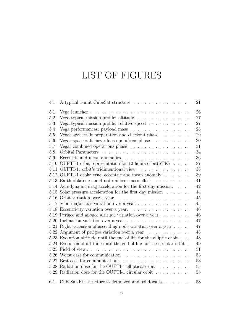
LIST OF FIGURES
4.1 A typical 1-unit CubeSat structure . . . . . . . . . . . . . . . . 21
5.1 Vega launcher . . . . . . . . . . . . . . . . . . . . . . . . . . . . 265.2 Vega typical mission profile: altitude . . . . . . . . . . . . . . . 275.3 Vega typical mission profile: relative speed . . . . . . . . . . . . 275.4 Vega performances: payload mass . . . . . . . . . . . . . . . . . 285.5 Vega: spacecraft preparation and checkout phase . . . . . . . . 295.6 Vega: spacecraft hazardous operations phase . . . . . . . . . . . 305.7 Vega: combined operations phase . . . . . . . . . . . . . . . . . 315.8 Orbital Parameters . . . . . . . . . . . . . . . . . . . . . . . . . 345.9 Eccentric and mean anomalies. . . . . . . . . . . . . . . . . . . 365.10 OUFTI-1 orbit representation for 12 hours orbit(STK) . . . . . 375.11 OUFTI-1: orbit’s tridimentional view. . . . . . . . . . . . . . . 385.12 OUFTI-1 orbit: true, eccentric and mean anomaly . . . . . . . . 395.13 Earth oblateness and not uniform mass effect . . . . . . . . . . 415.14 Aerodynamic drag acceleration for the first day mission. . . . . 425.15 Solar pressure acceleration for the first day mission . . . . . . . 445.16 Orbit variation over a year. . . . . . . . . . . . . . . . . . . . . 455.17 Semi-major axis variation over a year. . . . . . . . . . . . . . . . 455.18 Eccentricity variation over a year. . . . . . . . . . . . . . . . . . 465.19 Perigee and apogee altitude variation over a year. . . . . . . . . 465.20 Inclination variation over a year. . . . . . . . . . . . . . . . . . . 475.21 Right ascension of ascending node variation over a year . . . . . 475.22 Argument of perigee variation over a year . . . . . . . . . . . . 485.23 Evolution altitude until the end of life for the elliptic orbit . . . 485.24 Evolution of altitude until the end of life for the circular orbit . 495.25 Field of view . . . . . . . . . . . . . . . . . . . . . . . . . . . . . 515.26 Worst case for communication . . . . . . . . . . . . . . . . . . . 535.27 Best case for communication . . . . . . . . . . . . . . . . . . . . 535.28 Radiation dose for the OUFTI-1 elliptical orbit . . . . . . . . . 555.29 Radiation dose for the OUFTI-1 circular orbit . . . . . . . . . . 55
6.1 CubeSat-Kit structure skeletonized and solid-walls . . . . . . . . 58
9

6.2 ISIS structure . . . . . . . . . . . . . . . . . . . . . . . . . . . . 606.3 P-POD: deployment system for three CubeSats . . . . . . . . . 62
7.1 Example of OUFTI-1 configuration . . . . . . . . . . . . . . . . 647.2 Gravity gradient couple in case of non updated configuration . . 687.3 Aerodynamic couple in case of non updated configuration . . . . 697.4 Gravity gradient couple in case of updated configuration . . . . 707.5 Gravity gradient couple in case of updated configuration . . . . 70
8.1 Reference sistems . . . . . . . . . . . . . . . . . . . . . . . . . . 748.2 Sun rays direction on the ecliptic plane . . . . . . . . . . . . . . 758.3 Sun rays direction projected on the orbit plane. . . . . . . . . . 768.4 Eclipse duration as a function of earth anomaly . . . . . . . . . 778.5 Total power produced: simulation over one year orbit. . . . . . . 808.6 Integrated power: simulation over one year orbit . . . . . . . . . 808.7 Total power and integrated power for the orbital parameters after
one year mission . . . . . . . . . . . . . . . . . . . . . . . . . . . 818.8 Total power and integrated power for the circular orbit with Ω =
0 and ω = 0 . . . . . . . . . . . . . . . . . . . . . . . . . . . . . 828.9 Total power and integrated power for Ω = 90 and ω = 0 . . . . 838.10 Total power and integrated power for Ω = 0 and ω = 90 . . . . 838.11 Total power and integrated power for Ω = 90 and ω = 90 . . . 83
9.1 Nodes model for thermal analysis . . . . . . . . . . . . . . . . . 899.2 Equilibrium for radiative heat exchange . . . . . . . . . . . . . . 909.3 Radiative equivalent resistance . . . . . . . . . . . . . . . . . . . 919.4 Typical Thermal Excel layout: operating case whit black coating 94
10.1 Communication system block diagram . . . . . . . . . . . . . . 9810.2 Detailed link budget for the satellite at the apogee, 5 elevation 10210.3 Downlink link budget . . . . . . . . . . . . . . . . . . . . . . . . 103
11.1 Qualification level test for sinus vibrations . . . . . . . . . . . . 10811.2 Qualification level for random vibrations . . . . . . . . . . . . . 10911.3 Shock Response Spectrum . . . . . . . . . . . . . . . . . . . . . 109
10
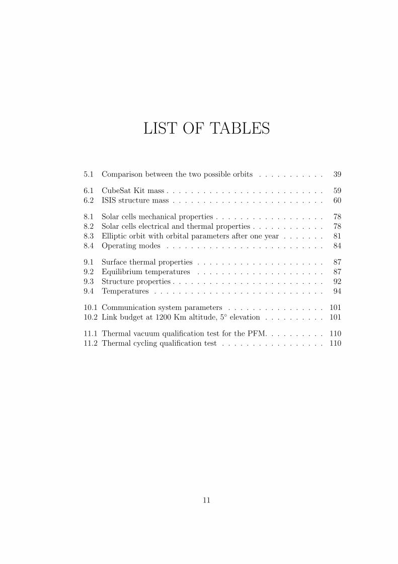
LIST OF TABLES
5.1 Comparison between the two possible orbits . . . . . . . . . . . 39
6.1 CubeSat Kit mass . . . . . . . . . . . . . . . . . . . . . . . . . . 596.2 ISIS structure mass . . . . . . . . . . . . . . . . . . . . . . . . . 60
8.1 Solar cells mechanical properties . . . . . . . . . . . . . . . . . . 788.2 Solar cells electrical and thermal properties . . . . . . . . . . . . 788.3 Elliptic orbit with orbital parameters after one year . . . . . . . 818.4 Operating modes . . . . . . . . . . . . . . . . . . . . . . . . . . 84
9.1 Surface thermal properties . . . . . . . . . . . . . . . . . . . . . 879.2 Equilibrium temperatures . . . . . . . . . . . . . . . . . . . . . 879.3 Structure properties . . . . . . . . . . . . . . . . . . . . . . . . . 929.4 Temperatures . . . . . . . . . . . . . . . . . . . . . . . . . . . . 94
10.1 Communication system parameters . . . . . . . . . . . . . . . . 10110.2 Link budget at 1200 Km altitude, 5 elevation . . . . . . . . . . 101
11.1 Thermal vacuum qualification test for the PFM. . . . . . . . . . 11011.2 Thermal cycling qualification test . . . . . . . . . . . . . . . . . 110
11

CHAPTER
1
INTRODUCTION
This work represents the feasibility study for the CubeSat OUFTI-1, the firststep of the LEODIUM Project of the University of Liege, Belgium.The goals of the project are soon introduced, as well as an explanation of theOUFTI-1 mission, including the concepts of CubeSat and amateur radio. Thena description of all the satellite subsystems is treated, with the attention concen-trated on the mission analysis. For each subsystem an analysis of the operationalconditions is carried out and the foreseen solutions are presented.We start with the mission analysis as it is the subsystem that mainly influencesall the others. We pass then to the structure and deployment system, that arecommercial off-the-shelf elements, and to the attitude control system, which isthe most controversial subsystem for the OUFTI-1 satellite project. Then astudy on the power produced in orbit is carried out to determine if we haveenough power to supply our satellite. Afterward the thermal system is intro-duced and the solutions to control the satellite temperature are presented. Thelast subsystem is the communication system which is especially important asit also represents the CubeSat payload: with a link budget we find out if thesatellite has enough power to communicate with the earth.At the end, the tests philosophy is explained and a choice of possible payloadsfor the future missions of LEODIUM Project is introduced.
13


CHAPTER
2
THE LEODIUM PROJECT
The LEODIUM Project is a project involving the University of Liege and LiegeEspace, a consortium of space industries and research centers in the Liege regionwith the goal of increase the cooperation between the members and to promotethe space activity.LEODIUM is the Latin name of Liege and stands for Lancement En Orbitede Demonstations Innovantes d’une Universite Multidisciplinaire (Launch intoOrbit of Innovative Demonstrations of a Multidisciplinary University). Theproject started in 2005 when Mr. Pierre Rochus, president of Liege Espace andDeputy General Manager for Space Instrumentation of the Liege Space Center,was charged with the training of students to the design of miniaturized satellites.Some possible scenarios to involve students in the design of a space mission wereforeseen and each one had its advantages and drawbacks:
• Design of a CubeSat or of a Nanosatellite: quick and relatively simple butwith a scientific payload not really efficient due to the low mass and poweravailable.
• Design of a Microsatellite: very interesting on the scientific point of viewbut requiring much more time and economical resources.
• Participation to the design of a space instrument among a professionalteam: interesting mission but less possibility to actively participate.
The project started with the participation in the Student Space Exploration andTechnology Initiative (SSETI) of the European Space Agency: the Universityof Liege took part in the European Student Earth Orbiter (ESEO) designing
15
CHAPTER 2
the solar panels deployment system and in the European Student Moon Orbiter(ESMO) developing the Narrow Angle Camera (NAC).The project of a nanosatellite was instead in a kind of stall until September2007 when Mr. Luc Halbach, sales manager of Spacebel, proposed the designof a CubeSat for amateur radio, equipped with a new digital technology: theD-STAR system. In less than one month, a team of students and professors wasgrouped and the design of the first CubeSat of the University of Liege started. Itwas called OUFTI-1 which is a typical expression of the city of Liege and whichstands for Orbiting Utility For Telecommunication Innovation. The project wenton and the idea of launching many CubeSats carrying scientific experimentsbecame more and more concrete: now the University of Liege has the ambitiousprogram of developing a series of CubeSats to give students hands-on experiencewith all the phases of the design and operation of a complete satellite system.A CubeSat is in fact the best mean to accomplish this educational mission: itsdesign goes on just like a traditional space mission but, being the development’stime much shorter, it gives students the opportunity of participating to all themission phases from the feasibility study to the launch.At the same time, the LEODIUM project will allow the space qualification ofsome recently-developed technologies and some scientific experiments on-boardof the futures CubeSats. In chapter 12, a more detailed description of thepossible payloads will be presented.Concerning OUFTI-1, its main goal is to demonstrate the feasibility of using theamateur radio D-STAR digital communication protocol to communicate with,and through, a CubeSat: it will be in fact the first satellite ever to use this kindof technology. If it works and it’s successfully space-tested, it will be the maincommunication system for all the next CubeSats of the Liege University.
Galli Stefania 16 University of Liege
CHAPTER
3
THE FLIGHT OPPORTUNITY
The Education Office of the European Space Agency (ESA), in cooperationwith the Directorate of Legal Affairs and External Relations and the Vega Pro-gramme Office in the Directorate of Launchers, issued a first AnnouncementOpportunity on 9 October 2007 offering a free launch on the Vega maiden flightfor six CubeSats. In the meantime, the Vega Maiden Flight CubeSat Workshopwas held at the European Space Research and Technology Center (ESTEC): theUniversity of Liege participated presenting the LEODIUM Project [RD1]. On15 February 2008, the ESA published a call for proposal for CubeSat on-boardof Vega [RD2] and on 17 mars 2008 the proposal was submitted to the ESA[RD3].Up to know, we are still waiting for an hopefully positive answer.
17

CHAPTER
4
THE CUBESAT OUFTI-1
OUFTI-1 is a CubeSat representing the first step of the LEODIUM Project:it’s also the first satellite of the University of Liege and the first Picosatelliteever made in Belgium. It’s an amateur radio satellite exploiting the digital-communication D-STAR protocol and it’s not going to carry any scientific pay-load but it will mainly be used as a test for the D-STAR system into space: itcan be viewed as a bare-bone repeater in space.Furthermore, the OUFTI-1 bus could be used in the future as standard plat-form for the next CubeSats of the University of Liege. As they will have somescientific experiments on-board, the use of an already tested platform will allowto concentrate the effort on the payload and on the mission analysis in orderto reach the target in the best way as possible. Moreover, once the scientificmission will have finished, the CubeSat will be used by the amateur radio com-munity: in return, we can communicate with the ground station trough thefrequency bandwidth reserved for the amateur radio communications.The main constraint for this mission is the time line: the launch is in factscheduled for December 2008 and the project started in November 2007. Evenif two years are considered sufficient for the design and operation of a CubeSatmission, we need to optimize the time and to proceed as quickly as possible.For this reason we assumed the principle of KISS, Keep It Simple and Stupid.We are in fact convinced that between two possible solutions that guarantee thesame final result, the most convenient is the simplest: guided by this idea, allthe choices are taken in order to simplify the design.Before proceeding with the satellite description, an introduction to the CubeSatconcept and to the D-STAR system is presented.
19
CHAPTER 4
4.1 The CubeSat concept
During the last years, a complex process is taking place in the space industry: onthe one hand, there is a growing tendency for satellite to become larger, on theother hand, many miniaturized satellites are designed. In fact, from the hugespacecraft of Hubble Space Telescope launched in 1990 which weighed morethan 11 tons, there is an actual trend to reduce at most the size of the satellite:this reduces not only the costs connected to the launch but also those directlyimplied in the design and construction of the spacecraft. The miniaturizedsatellite can be classified according to their ’wet’ mass (including fuel) :
• Minisatellite: wet mass between 100 Kg and 500 Kg. They are usuallysimple but they use the same technology as the bigger satellites and theyare often equipped with rockets for propulsion and attitude control.
• Microsatellite: wet mass between 10 Kg and 100 Kg. The miniaturizationprocess begins to be important but sometimes they still use some kind ofpropulsion.
• Nanosatellite: wet mass between 1 Kg and 10 Kg. Every component hasto be reduced in terms of mass and volume and no kind of propulsion isusually foreseen. They can be launched ’piggyback’, using excess capabil-ity on larger launch vehicle.
• Picosatellite: wet mass between 0.1 Kg et 1 Kg. The miniaturizationprocess is maximum and many new technologies have to be used in orderto accomplish the requirements. They are launched ’piggyback’ with somepeculiar deployment system.
These miniaturized satellites go toward many technical challenges, especiallyconcerning the attitude control and the electronic equipment, including thecommunication system: they need indeed to use more up-to-date technology,which often needs to be carefully tested and modified in order to be space hard-ened and resistant to the outer space environment.
The CubeSat design is an example of a Picosatellite with dimensions of10x10x10 cm and typically using commercial off-the-shelf electronic compo-nents. The concept was originally developed by the California Polytechnic StateUniversity and by the Stanford University, with Professor Robert Twiggs, andafterward it widely circulates among the academic world . At the moment, over60 University, high schools and industries are involved in the development ofCubeSats. Some of them are designing double and triple CubeSats: they can fitin the traditional deployment system but they can have more mass and volume.As a matter of fact, a CubeSat represents the best way to give some experience
Galli Stefania 20 University of Liege
CHAPTER 4. THE CUBESAT OUFTI-1
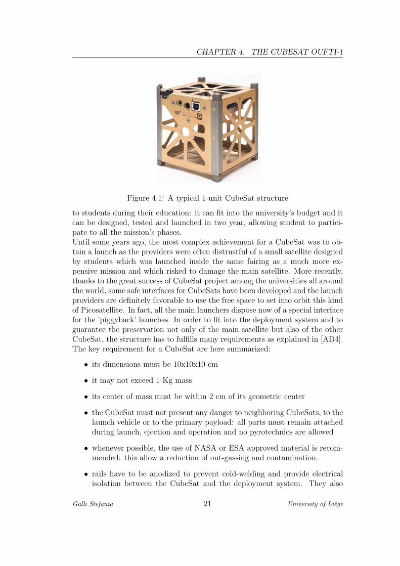
Figure 4.1: A typical 1-unit CubeSat structure
to students during their education: it can fit into the university’s budget and itcan be designed, tested and launched in two year, allowing student to partici-pate to all the mission’s phases.Until some years ago, the most complex achievement for a CubeSat was to ob-tain a launch as the providers were often distrustful of a small satellite designedby students which was launched inside the same fairing as a much more ex-pensive mission and which risked to damage the main satellite. More recently,thanks to the great success of CubeSat project among the universities all aroundthe world, some safe interfaces for CubeSats have been developed and the launchproviders are definitely favorable to use the free space to set into orbit this kindof Picosatellite. In fact, all the main launchers dispose now of a special interfacefor the ’piggyback’ launches. In order to fit into the deployment system and toguarantee the preservation not only of the main satellite but also of the otherCubeSat, the structure has to fulfills many requirements as explained in [AD4].The key requirement for a CubeSat are here summarized:
• its dimensions must be 10x10x10 cm
• it may not exceed 1 Kg mass
• its center of mass must be within 2 cm of its geometric center
• the CubeSat must not present any danger to neighboring CubeSats, to thelaunch vehicle or to the primary payload: all parts must remain attachedduring launch, ejection and operation and no pyrotechnics are allowed
• whenever possible, the use of NASA or ESA approved material is recom-mended: this allow a reduction of out-gassing and contamination.
• rails have to be anodized to prevent cold-welding and provide electricalisolation between the CubeSat and the deployment system. They also
Galli Stefania 21 University of Liege

CHAPTER 4
have to be smooth and their edges rounded
• the use of Aluminium 7075 or 6061-T6 is suggested for the main structure.If others materials are used, the thermal expansion must be similar to thatof the deployment system material (Aluminium 7075-T73) and approved.This prevents the CubeSat to conk out because of an excessive thermaldilatation.
• no electronic device may be active during launch. Rechargeable batterieshave to be discharged or the CubeSat must be fully deactivated
• at least one deployment switch is required
• antennas can be deployed only 15 minutes after ejection into orbit whilebooms and solar panels after 30 minutes
• it has to undergo qualification and acceptance testing according to thespecifications of the launcher: at least random vibration testing at a levelhigher than the published launch vehicle envelope and thermal vacuumtesting. Each CubeSat has to survive qualification testing for the specificlauncher. Acceptance testing will also be performed after the integrationinto the deployment system.
4.1.1 Amateur Radio and D-STAR system
Before proceeding with the description of OUFTI-1, a brief introduction of thesatellite’s payload, represented by its communications system, is necessary.D-STAR, which stands for Digital Smart Technology for Amateur Radio, isan open ham radio protocol recently developed by the Japan Amateur RadioLeague (JARL). Its main features are the simultaneous transmission of voiceand data, the complete routing capacity (including roaming), the cross-bandcapability and the possibility of passing through the internet.It works over three possible frequencies and data rates:
• 144 MHz ( 2m, VHF ), 4.8 Kbit/s
• 440 MHz ( 70 cm, UHF ), 4.8 Kbit/s
• 1.2 GHz ( 23 cm, SHF ), 4.8 Kbit/s or 128 Kbit/s
Presently, in Europe only the first two frequencies are available.The D-STAR technology is in fact really developed in the United States, wheremany repeaters are operational, but it’s quickly extending in Europe: the firstrepeater in Belgium is at the University of Liege and it has been installed withinthe OUFTI-1 project.
Galli Stefania 22 University of Liege

CHAPTER 4. THE CUBESAT OUFTI-1
The idea of using a satellite for amateur radio communication is not new: thefirst ham radio satellite OSCAR-1 has been launched in 1961 and OSCAR-7,launched in 1974, is still operational. Many satellites for radio amateurs arein low earth orbit and guarantee the communications all around the world:even on the International Space Station (ISS) there is a amateur radio stationand a new one has been recently added on the Columbus module. The reasonis simple: in normal atmospheric conditions the zone of visibility of a radiorepeater is around 50 Km, while the footprint of a satellite is much wider (orderof thousands Km): a satellite allows in this way the communication between twousers far away from each other and, even more important, it offers a repeaterto those who are to far away from any ground repeaters to have a traditionalair link.As a drawback, both the two users have to be in the satellite footprint and thetime for communicate could be short.During the last months, OUFTI-1 has been presented to the amateur radiocommunity and to other CubeSats developers [RD4] and it has been greetedenthusiastically.
Galli Stefania 23 University of Liege

CHAPTER
5
MISSION ANALYSIS
The mission analysis is the process of quantifying the system parameters andthe resulting performance: its main goal is to analyse whether the mission meetsthe requirements or not.The first step is therefore to define the mission requirements. In this case, due tothe absence of a scientific payload, the only real requirement is to guarantee tothe amateur radio operators a sufficient communication time with a convenientquality. Being the amateur radio operators common all around the world, wechose as main criteria a passing time over Belgium as longer as possible: thisfavor the Belgian amateur radio operators, which seems logical as the CubeSatis Belgian, but guarantees also a sufficient passing time of the spacecraft in viewof the ground station in Liege. Concerning the lifetime, the goal is to ensureenough operating time to successfully test the D-STAR system but, also in thiscase, we are not able to quantify it.The reason of this lack of mission requirements is simple: on the one hand,the ESA offers free launch on board the Vega launcher but it imposes the orbitand, on the other hand, a CubeSat needs to meet some requirements in termsof mass, size, shape and pyrotechnics.We cannot therefore neither choose an orbit that guarantees a longer lifetimeand a sufficient passing time over Belgium, nor add any kind of propulsion, noradopt any peculiar shape of the structure. The only thing that we can do, isto use the available mass and size as good as possible, in order to screen thesensible equipments from the radiation, and to choose omnidirectional antennasto communicate as long as possible with the small amount of power producedin orbit.
25
CHAPTER 5
5.1 The Vega Launcher
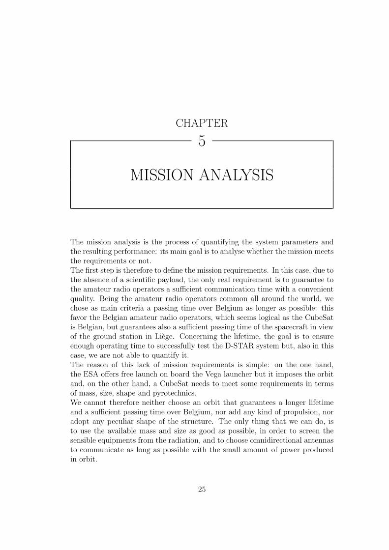
Vega, Vettore Europeo di Generazione Avanzata, is the new European smalllauncher. It has been designed as a single body launcher with three solidpropulsion stages and an additional liquid propulsion restartable upper mod-ule, AVUM, used for attitude and orbit control and for satellite release. Unlikemost small launchers, Vega will be able to place multiple payloads into orbit.Its development started in 1998 and the first flight was initially expected in2007 from the Guyana Space Center, CSG, but different reasons causes somedelays and, up to know, it is scheduled for the December 2008.It is funded by Belgium, France, Italy, Spain, Sweden, Switzerland and TheNetherlands.Vega is 30 m high, has a maximum diameter of 3 m and weights 137 tons atlift-off. As shown in fig.5.1, it has three sections: the Lower Composite, theUpper Composite known as AVUM and the Payload Composite.
Figure 5.1: Vega launcher
Galli Stefania 26 University of Liege

CHAPTER 5. MISSION ANALYSIS
5.1.1 Typical Mission Profile
A typical mission profile consists of three phases:
• Phase I: Ascent of the first three stages of the launch vehicle into the lowelliptic trajectory (sub-orbital profile)
• Phase II: Payload and upper stage transfer to the initial parking orbitby first AVUM burn, orbital passive flight and orbital manoeuvres of theAVUM stage for payload delivery to final orbit
• Phase III: AVUM deorbitation or orbit disposal manoeuvres.
Figure 5.2: Vega typical mission profile: altitude as a function of time after liftoff.
Figure 5.3: Vega typical mission profile: relative speed as a function of timeafter lift off.
Galli Stefania 27 University of Liege

CHAPTER 5
Typically, the AVUM burns three times: the first to place the satellite andhimself into an elliptical orbit with the apogee at the target altitude, the secondto raise the perigee to the required value or for orbit circularization and thethird for deorbiting himself. Jettisoning of the payload fairing can take place atdifferent times, depending on the aero-thermal flux requirements on the payload,but normally it happens between 200 and 260 seconds from lift-off.
5.1.2 Performances
Vega is designed to launch a wide range of missions and payload configuration:in particular, it can place in to orbit masses ranging from 300 to 2500 Kg intoa variety of orbit, from equatorial, to sun synchronous and polar. Its perfor-mances are shown in figure 5.4.
Figure 5.4: Vega performances: payload mass as a function of orbit inclinationand altitude required.
Vega can also operate the launch of multiple payloads.
5.1.3 Launch Campaign
The spacecraft launch campaign formally begins with the delivery in CSG of thespacecraft and its associated Ground Support Equipments (GSE), and concludeswith GSE shipment after launch. It cannot exceed 30 days: 27 days beforelaunch and 3 days after it.A typical launch campaign can be divided in three parts:
1. Spacecraft autonomous preparationIt includes all the operations conducted from the spacecraft arrival to theCSG up to the readiness for integration with the launch vehicle.
Galli Stefania 28 University of Liege
CHAPTER 5. MISSION ANALYSIS
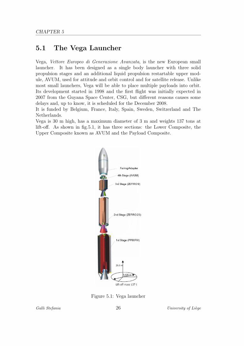
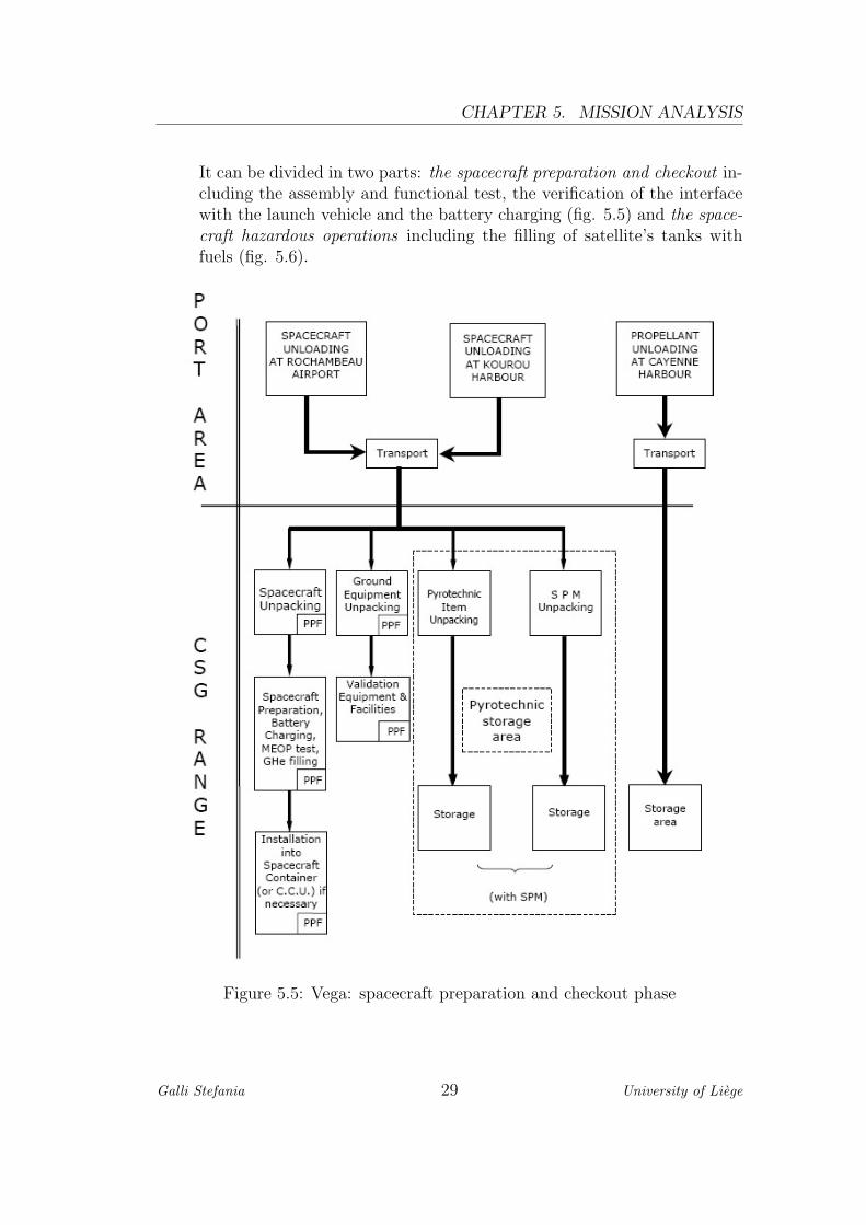
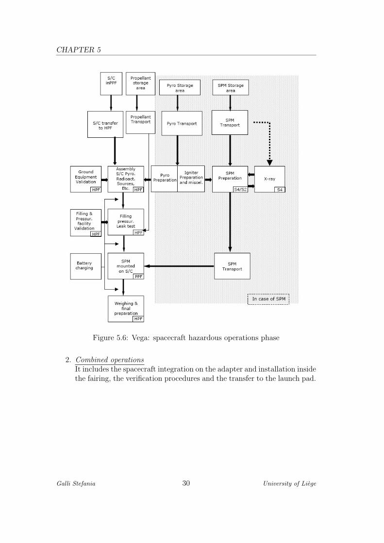
It can be divided in two parts: the spacecraft preparation and checkout in-cluding the assembly and functional test, the verification of the interfacewith the launch vehicle and the battery charging (fig. 5.5) and the space-craft hazardous operations including the filling of satellite’s tanks withfuels (fig. 5.6).
Figure 5.5: Vega: spacecraft preparation and checkout phase
Galli Stefania 29 University of Liege
CHAPTER 5
Figure 5.6: Vega: spacecraft hazardous operations phase
2. Combined operationsIt includes the spacecraft integration on the adapter and installation insidethe fairing, the verification procedures and the transfer to the launch pad.
Galli Stefania 30 University of Liege
CHAPTER 5. MISSION ANALYSIS
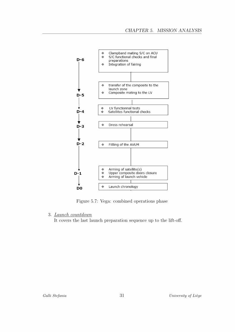
Figure 5.7: Vega: combined operations phase
3. Launch countdownIt covers the last launch preparation sequence up to the lift-off.
Galli Stefania 31 University of Liege

CHAPTER 5
5.1.4 The Vega Maiden Flight
The Vega maiden flight is targeted officially targeted for December 2008: theprimary scientific payload is the LAser RElativity Satellite (LARES). Its anitalian satellite, designed by the Italian Space Agency (ASI) in cooperation withthe University of Rome testing a prediction following from the Einstein’s theoryof General Relativity, the so-called ‘frame-dragging or Lense-Thirring effect’.It’s basically a solid sphere maid of Tungsten with a diameter of 376 mm anda mass of 400 Kg. The surface is covered by 92 Corner Cube Reflectors (CCR)which, hit by laser beams sent from earth, will reflect them allowing an accurateorbit determination. Correcting for a number of effects, most importantly thedeviation of the earth gravitational field from an ideal sphere, yields the frame-dragging effect. To achieve its scientific objectives, LARES needs to be injectedinto a circular orbit at 1200 Km altitude with an inclination of 71.Furthermore, an adaptation of the Upper Composite test dummy used duringmechanical test campaign will be the main passenger on the Vega maiden flight:it will measure the actual launch loads experienced by a typical payload in orderto correlate them with the numerical models used during the launcher’s designphase.Besides, an educational payload of six CubeSat, placed into two PicosatelliteOrbital Deployers (POD), will be accommodated into the fairing. They willbe released in a 1200x350 Km elliptical orbit thanks to the AVUM multi-burnfacility. A manoeuvre into a circular orbit at 350 Km altitude is also understudy. Both these two orbit guarantees a lifetime much less than 25 years,compliant with the international requirement related to space debris.
Galli Stefania 32 University of Liege
CHAPTER 5. MISSION ANALYSIS
5.2 The orbit
The choice of the orbit is an important step in every space mission as it stronglyinfluences the final performances. It’s usually driven by the missions require-ments and therefore it’s specific for each satellite. In this case, as the CubeSatsare secondary payloads on the Vega maiden flight, we couldn’t set anyway theorbit parameter as they are determined by its main payload, the LARES ex-periment.As above-mentioned, the foreseen orbit is elliptical with a perigee at 350 Kmaltitude, an apogee at 1200 Km and an inclination of 71. Concerning the argu-ment of perigee and the right ascension of ascending node, any input hasn’t beenassigned yet. As the LARES satellite will be placed into a circular orbit, theargument of perigee is the only parameters that can be influenced by the Cube-Sat requirements. Considering that all the CubeSats are european and thatthey necessary have their main ground stations in the northern hemisphere, weexpect and hope to have the apogee over the northern hemisphere: in this case,we could have the longest time to use OUFTI-1 as amateur radio repeater overEurope and to communicate with our ground station. As shown in paragraph5.3.4, the argument of perigee is changing during the satellite lifetime but, asthe D-STAR system has never been used into space and as we still don’t knowhow long it will able to work before breaking down, we strongly hope that itwill be in a convenient position at the beginning.Concerning the possibility of a circular orbit at 350 Km altitude, it’s not thebest solution for OUFTI-1 and , more in general, for the CubeSats: on theone hand, the communication time with the ground stations is short, even ifit’s better than for the case of elliptic orbit with the perigee over the northernhemisphere, and, on the other hand, the lifetime is extremely brief.Anyway, as the most probable orbit is the elliptic one, we will perform theanalysis basing on it, which also represent the more general case.Before describing the OUFTI-1 orbit, we proceed with a recall of orbital me-chanics.
5.2.1 Orbital mechanics
The orbital mechanics studies the motion of a spacecraft on a specific trajectory,called orbit, basing on the Newton’s laws of motion and of universal gravitation.Directly from them, come the three Kepler’s laws of planetary motion:
- The orbit of every planet is an ellipse with the sun at one of the foci.
- The line joining a planet and the sun sweeps out equal areas during equalintervals of time as the planet travels around its orbit.
Galli Stefania 33 University of Liege
CHAPTER 5
- The squares of the orbital period of planets are directly proportional tothe cube of the semi-major axes of their orbit.
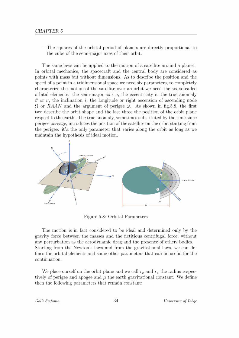
The same laws can be applied to the motion of a satellite around a planet.In orbital mechanics, the spacecraft and the central body are considered aspoints with mass but without dimensions. As to describe the position and thespeed of a point in a tridimensional space we need six parameters, to completelycharacterize the motion of the satellite over an orbit we need the six so-calledorbital elements: the semi-major axis a, the eccentricity e, the true anomalyϑ or ν, the inclination i, the longitude or right ascension of ascending nodeΩ or RAAN and the argument of perigee ω. As shown in fig.5.8, the firsttwo describe the orbit shape and the last three the position of the orbit planerespect to the earth. The true anomaly, sometimes substituted by the time sinceperigee passage, introduces the position of the satellite on the orbit starting fromthe perigee: it’a the only parameter that varies along the orbit as long as wemaintain the hypothesis of ideal motion.
Figure 5.8: Orbital Parameters
The motion is in fact considered to be ideal and determined only by thegravity force between the masses and the fictitious centrifugal force, withoutany perturbation as the aerodynamic drag and the presence of others bodies.Starting from the Newton’s laws and from the gravitational laws, we can de-fines the orbital elements and some other parameters that can be useful for thecontinuation.
We place ourself on the orbit plane and we call rp and ra the radius respec-tively of perigee and apogee and µ the earth gravitational constant. We definethen the following parameters that remain constant:
Galli Stefania 34 University of Liege
CHAPTER 5. MISSION ANALYSIS
• the semi-major axis:
a =rp + ra
2(5.1)
• the eccentricity:
e =ra − rp
ra + rp
(5.2)
• the angular momentum and its magnitude:
h = r× v h = |h| = rvcos(γ) (5.3)
where r is the radius, v the speed and γ the flight angle.
• the orbit parameter which represents the radius of the circular orbit havingthe same angular momentum:
p = a(1− e2
)=
h2
µ= rc (5.4)
• the speed on the circular orbit having the same angular momentum:
vc =µ
h(5.5)
• the energy
E = − µ
2a=
v2
2− µ
r(5.6)
where v and r are the magnitude of speed and the radius.
• the period
T = 2π
√a3
µ(5.7)
Introducing the true anomaly ϑ we can identify the radius on each orbitpoint:
r =p
1 + ecos(ϑ)(5.8)
Galli Stefania 35 University of Liege
CHAPTER 5
Hence, the perigee and apogee radius can be expressed as:
rp = r (ϑ = 0) =p
1 + e= a (1− e) (5.9)
rp = r (ϑ = π) =p
1− e= a (1 + e) (5.10)
We would also like to find a connection between the time and the true anom-aly in order to know the necessary time to go from a point to another: if this isextremely simple for a circular orbit where the speed is constant, for an ellipticorbit it’s a bit more complicate.To solve this, Kepler introduced the quantity M, called mean anomaly, whichrepresents the fraction of an orbit period which has elapsed since perigee, ex-pressed as an angle:
M −M0 = n (t− t0) (5.11)
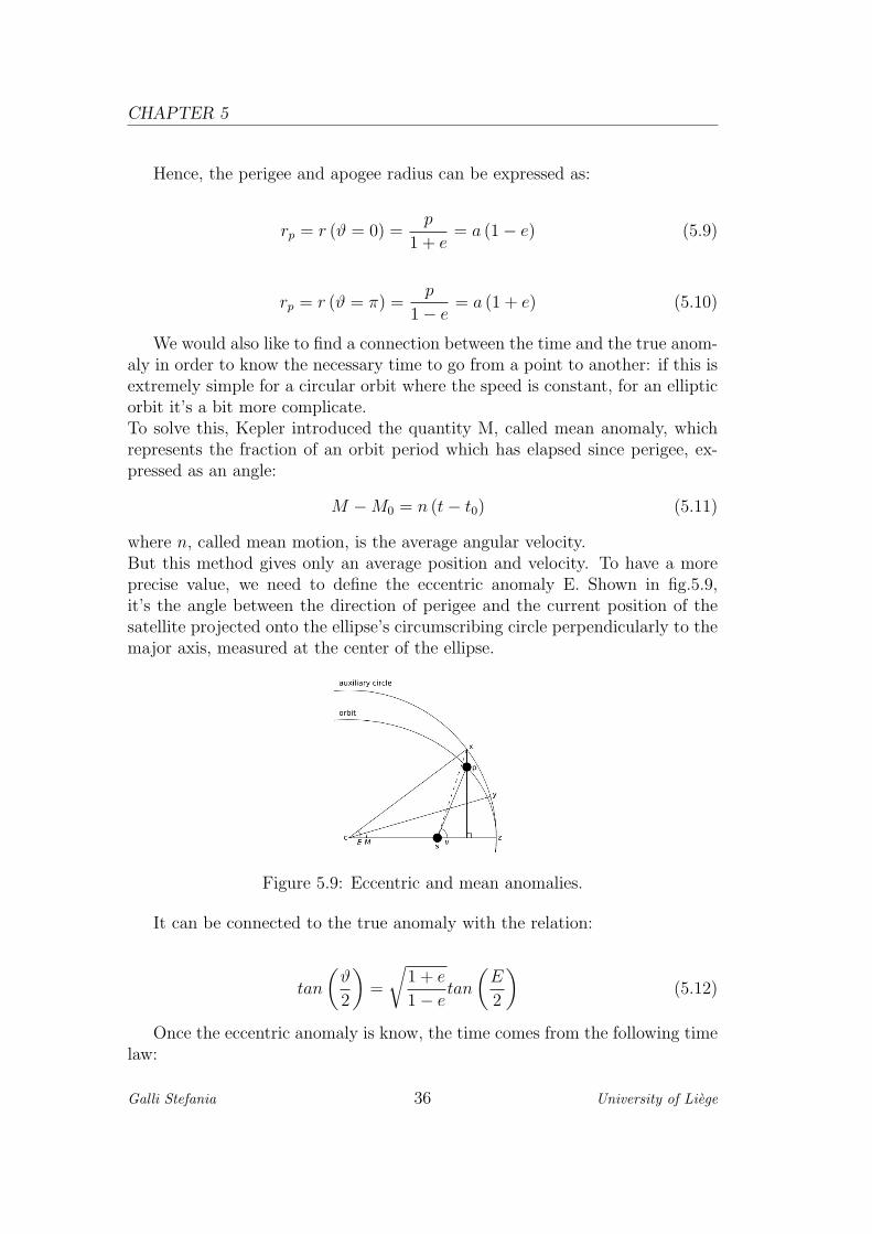
where n, called mean motion, is the average angular velocity.But this method gives only an average position and velocity. To have a moreprecise value, we need to define the eccentric anomaly E. Shown in fig.5.9,it’s the angle between the direction of perigee and the current position of thesatellite projected onto the ellipse’s circumscribing circle perpendicularly to themajor axis, measured at the center of the ellipse.
Figure 5.9: Eccentric and mean anomalies.
It can be connected to the true anomaly with the relation:
tan
(ϑ
2
)=
√1 + e
1− etan
(E
2
)(5.12)
Once the eccentric anomaly is know, the time comes from the following timelaw:
Galli Stefania 36 University of Liege

CHAPTER 5. MISSION ANALYSIS
t− t0 =
√a3
µ(E − esin (E)) (5.13)
5.2.2 The orbit of OUFTI-1
For the orbital analysis, we used some home-maid Matlab programs and theSTK software.As above mentioned, the following parameters are assigned:
• Perigee altitude: rp=350 Km
• Apogee altitude: ra=1200 Km
• Inclination : i=71
In order to have an idea of the orbit, we represented its ground track infig.5.10 and a tridimentional view in figure 5.11.
Figure 5.10: OUFTI-1 orbit representation for 12 hours orbit(STK)
Galli Stefania 37 University of Liege

CHAPTER 5
Figure 5.11: OUFTI-1: orbit’s tridimentional view. Optimum case: the sub-satellite point at apogee is at the same latitude as Liege.
Given a perigee of 350 Km and an apogee of 1200 Km altitude, we calculatedall the above mentioned parameters:
• semi-major axis: a = 7153.14Km
• eccentricity: e = 0.0594
• angular momentum: h = 5.33 · 104 Km2
s
• orbit parameter: p = 7127.7Km
• energy: E = −27.8Km2
s2
• period: T = 6020.8s = 100.35min
• perigee speed: vp = 7.922Kms
• apogee speed: va = 7.034Kms
• mean motion: n = 14.35 revday
Galli Stefania 38 University of Liege
CHAPTER 5. MISSION ANALYSIS
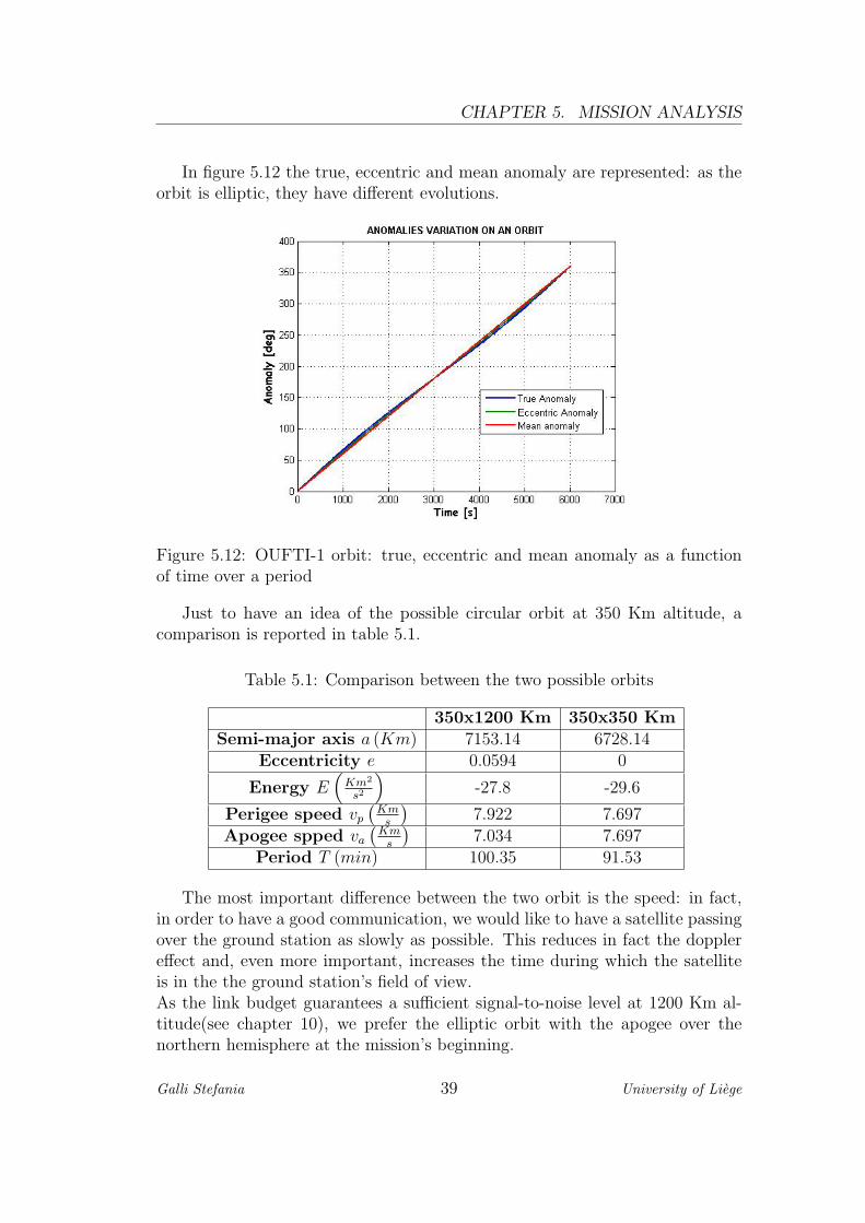
In figure 5.12 the true, eccentric and mean anomaly are represented: as theorbit is elliptic, they have different evolutions.
Figure 5.12: OUFTI-1 orbit: true, eccentric and mean anomaly as a functionof time over a period
Just to have an idea of the possible circular orbit at 350 Km altitude, acomparison is reported in table 5.1.
Table 5.1: Comparison between the two possible orbits
350x1200 Km 350x350 KmSemi-major axis a (Km) 7153.14 6728.14
Eccentricity e 0.0594 0
Energy E(
Km2
s2
)-27.8 -29.6
Perigee speed vp
(Km
s
)7.922 7.697
Apogee spped va
(Km
s
)7.034 7.697
Period T (min) 100.35 91.53
The most important difference between the two orbit is the speed: in fact,in order to have a good communication, we would like to have a satellite passingover the ground station as slowly as possible. This reduces in fact the dopplereffect and, even more important, increases the time during which the satelliteis in the the ground station’s field of view.As the link budget guarantees a sufficient signal-to-noise level at 1200 Km al-titude(see chapter 10), we prefer the elliptic orbit with the apogee over thenorthern hemisphere at the mission’s beginning.
Galli Stefania 39 University of Liege
CHAPTER 5
5.3 Orbit perturbations
The Keplerian orbit, considering only the earth gravitational force and thesatellite fictitious centrifugal force, provides an excellent reference but, for amore accurate study, we need to take into account some minor effects thatmake deviate the nominal orbit.We classify these variations of orbital elements in three main categories:
• the secular variations : they are a linear variation of the element. Theireffect cumulates in time and therefore they are the cause of changing shapeand orientation of the orbit.
• the long-period variations : they are those with a period greater than theorbital period.
• the short-period variations : they have a period less than the orbital period.They can usually be neglected.
In the sequel, three main effects will be considered: the earth’s oblateness, theatmospheric drag and the solar radiation pressure.
5.3.1 The earth’s oblateness
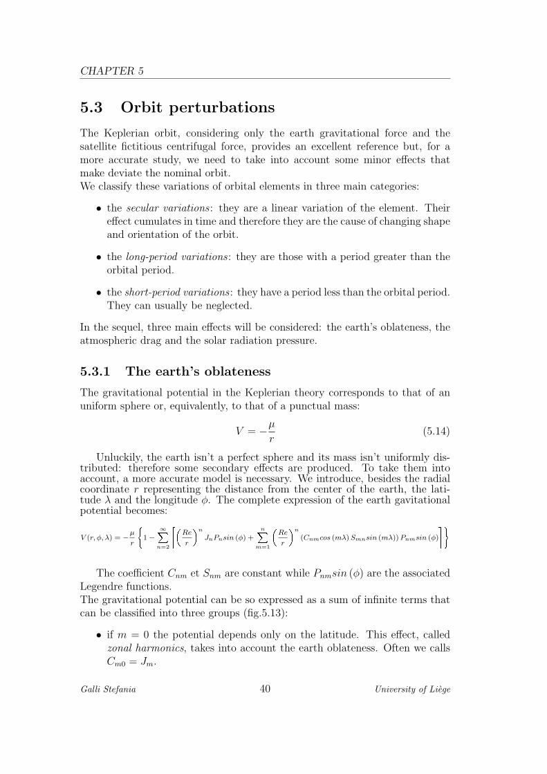
The gravitational potential in the Keplerian theory corresponds to that of anuniform sphere or, equivalently, to that of a punctual mass:
V = −µ
r(5.14)
Unluckily, the earth isn’t a perfect sphere and its mass isn’t uniformly dis-tributed: therefore some secondary effects are produced. To take them intoaccount, a more accurate model is necessary. We introduce, besides the radialcoordinate r representing the distance from the center of the earth, the lati-tude λ and the longitude φ. The complete expression of the earth gavitationalpotential becomes:
V (r, φ, λ) = −µ
r
(1−
∞Xn=2
"Re
r
n
JnPnsin (φ) +
nXm=1
Re
r
n
(Cnmcos (mλ) Smnsin (mλ)) Pnmsin (φ)
#)
The coefficient Cnm et Snm are constant while Pnmsin (φ) are the associatedLegendre functions.The gravitational potential can be so expressed as a sum of infinite terms thatcan be classified into three groups (fig.5.13):
• if m = 0 the potential depends only on the latitude. This effect, calledzonal harmonics, takes into account the earth oblateness. Often we callsCm0 = Jm.
Galli Stefania 40 University of Liege
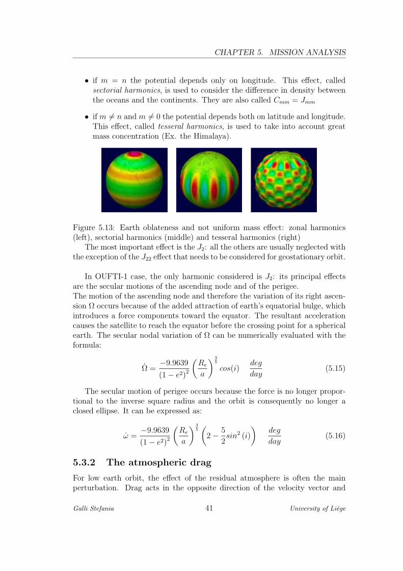
CHAPTER 5. MISSION ANALYSIS
• if m = n the potential depends only on longitude. This effect, calledsectorial harmonics, is used to consider the difference in density betweenthe oceans and the continents. They are also called Cmm = Jmm
• if m 6= n and m 6= 0 the potential depends both on latitude and longitude.This effect, called tesseral harmonics, is used to take into account greatmass concentration (Ex. the Himalaya).
Figure 5.13: Earth oblateness and not uniform mass effect: zonal harmonics(left), sectorial harmonics (middle) and tesseral harmonics (right)
The most important effect is the J2: all the others are usually neglected withthe exception of the J22 effect that needs to be considered for geostationary orbit.
In OUFTI-1 case, the only harmonic considered is J2: its principal effectsare the secular motions of the ascending node and of the perigee.The motion of the ascending node and therefore the variation of its right ascen-sion Ω occurs because of the added attraction of earth’s equatorial bulge, whichintroduces a force components toward the equator. The resultant accelerationcauses the satellite to reach the equator before the crossing point for a sphericalearth. The secular nodal variation of Ω can be numerically evaluated with theformula:
Ω =−9.9639
(1− e2)2
(Re
a
) 35
cos(i)deg
day(5.15)
The secular motion of perigee occurs because the force is no longer propor-tional to the inverse square radius and the orbit is consequently no longer aclosed ellipse. It can be expressed as:
ω =−9.9639
(1− e2)2
(Re
a
) 35(
2− 5
2sin2 (i)
)deg
day(5.16)
5.3.2 The atmospheric drag
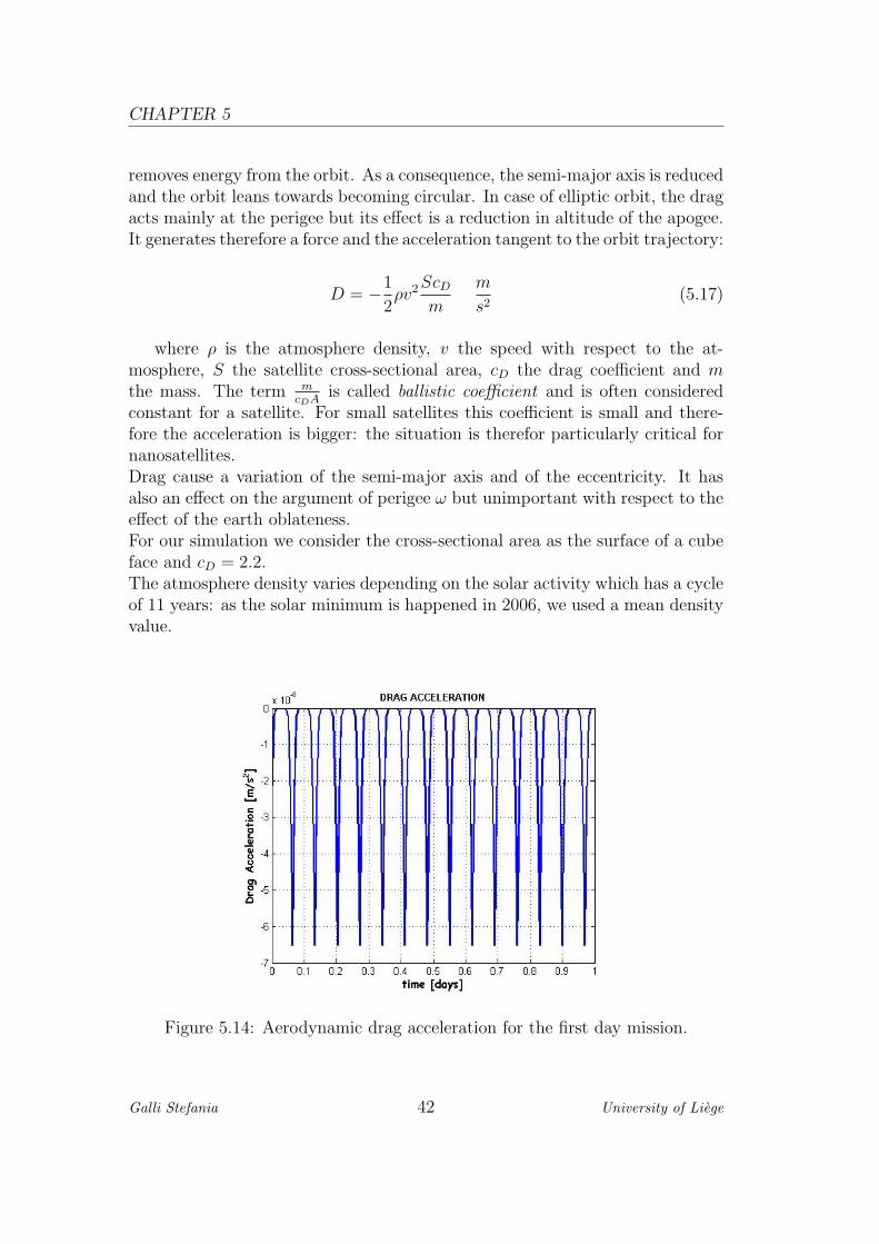
For low earth orbit, the effect of the residual atmosphere is often the mainperturbation. Drag acts in the opposite direction of the velocity vector and
Galli Stefania 41 University of Liege
CHAPTER 5
removes energy from the orbit. As a consequence, the semi-major axis is reducedand the orbit leans towards becoming circular. In case of elliptic orbit, the dragacts mainly at the perigee but its effect is a reduction in altitude of the apogee.It generates therefore a force and the acceleration tangent to the orbit trajectory:
D = −1
2ρv2ScD
m
m
s2(5.17)
where ρ is the atmosphere density, v the speed with respect to the at-mosphere, S the satellite cross-sectional area, cD the drag coefficient and mthe mass. The term m
cDAis called ballistic coefficient and is often considered
constant for a satellite. For small satellites this coefficient is small and there-fore the acceleration is bigger: the situation is therefor particularly critical fornanosatellites.Drag cause a variation of the semi-major axis and of the eccentricity. It hasalso an effect on the argument of perigee ω but unimportant with respect to theeffect of the earth oblateness.For our simulation we consider the cross-sectional area as the surface of a cubeface and cD = 2.2.The atmosphere density varies depending on the solar activity which has a cycleof 11 years: as the solar minimum is happened in 2006, we used a mean densityvalue.
Figure 5.14: Aerodynamic drag acceleration for the first day mission.
Galli Stefania 42 University of Liege
CHAPTER 5. MISSION ANALYSIS
5.3.3 The solar radiation pressure
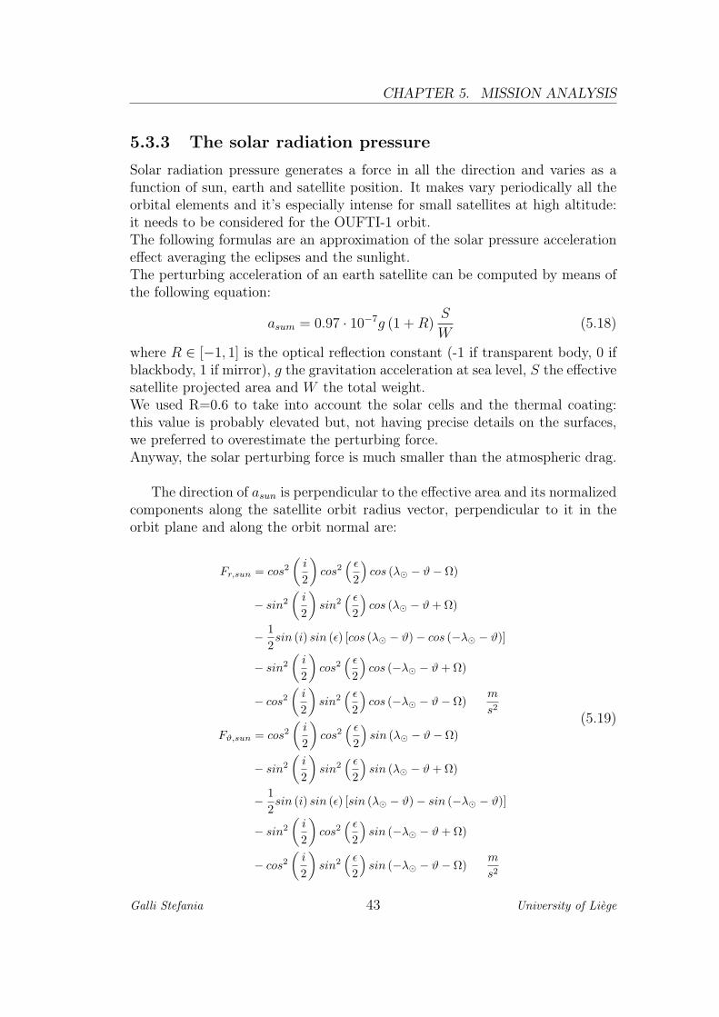
Solar radiation pressure generates a force in all the direction and varies as afunction of sun, earth and satellite position. It makes vary periodically all theorbital elements and it’s especially intense for small satellites at high altitude:it needs to be considered for the OUFTI-1 orbit.The following formulas are an approximation of the solar pressure accelerationeffect averaging the eclipses and the sunlight.The perturbing acceleration of an earth satellite can be computed by means ofthe following equation:
asum = 0.97 · 10−7g (1 + R)S
W(5.18)
where R ∈ [−1, 1] is the optical reflection constant (-1 if transparent body, 0 ifblackbody, 1 if mirror), g the gravitation acceleration at sea level, S the effectivesatellite projected area and W the total weight.We used R=0.6 to take into account the solar cells and the thermal coating:this value is probably elevated but, not having precise details on the surfaces,we preferred to overestimate the perturbing force.Anyway, the solar perturbing force is much smaller than the atmospheric drag.
The direction of asun is perpendicular to the effective area and its normalizedcomponents along the satellite orbit radius vector, perpendicular to it in theorbit plane and along the orbit normal are:
Fr,sun = cos2
(i
2
)cos2
( ε
2
)cos (λ − ϑ− Ω)
− sin2
(i
2
)sin2
( ε
2
)cos (λ − ϑ + Ω)
− 12sin (i) sin (ε) [cos (λ − ϑ)− cos (−λ − ϑ)]
− sin2
(i
2
)cos2
( ε
2
)cos (−λ − ϑ + Ω)
− cos2
(i
2
)sin2
( ε
2
)cos (−λ − ϑ− Ω)
m
s2
Fϑ,sun = cos2
(i
2
)cos2
( ε
2
)sin (λ − ϑ− Ω)
− sin2
(i
2
)sin2
( ε
2
)sin (λ − ϑ + Ω)
− 12sin (i) sin (ε) [sin (λ − ϑ)− sin (−λ − ϑ)]
− sin2
(i
2
)cos2
( ε
2
)sin (−λ − ϑ + Ω)
− cos2
(i
2
)sin2
( ε
2
)sin (−λ − ϑ− Ω)
m
s2
(5.19)
Galli Stefania 43 University of Liege
CHAPTER 5
F⊥,sun = sin (i) cos2( ε
2
)sin (λ − Ω)− sin (i) sin2
( ε
2
)sin (λ + Ω)
− cos (i) sin (ε) sin (λ)m
s2
where:
d = MJD − 150195.5
epsilon = 23.44
M = 358.48 + 0.98560027d
λ = 279.70 + 0.9856473d + 1.92sin(M)
MJD is the Modified Julian Date: Julian Date - 2400000.5.As shown in figure 5.15 this acceleration is much less intense than the one causedby the aerodynamic drag.
Figure 5.15: Solar pressure acceleration for the first day mission
5.3.4 Orbital parameters variation
The acceleration obtained above for the solar pressure and the atmosphere dragcan be used the quantify the variation of orbital elements:
a = 2a2
µvft
e = 2v(e + cos (ϑ)) ft − r
avsin (ϑ) fn
i = rhcos (ϑ∗) f⊥
eω = 2sin(ϑ)v
ft +(2e + r
asin (ϑ)
)1vfn − eΩcos (i)
Ωsin (i) = rhsin (ϑ∗) f⊥
(5.20)
Galli Stefania 44 University of Liege

CHAPTER 5. MISSION ANALYSIS
where ϑ∗ = ϑ − ω. ft, fn, f⊥ are the acceleration respectively tangent andnormal to the orbit in the orbital plane and normal to the orbital plane.This acceleration are the integrated in order to have the parameters variation.The effect of earth’s oblateness on Ω and ω is calculated and directly added.The results for the OUFTI-1 orbit over one year obtained with Matlab and withSTK are here presented:
Figure 5.16: Orbit variation over a year.
Figure 5.17: Semi-major axis variation over a year.
Galli Stefania 45 University of Liege
CHAPTER 5
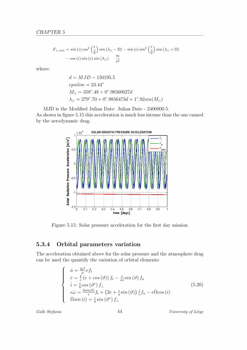
Figure 5.18: Eccentricity variation over a year.
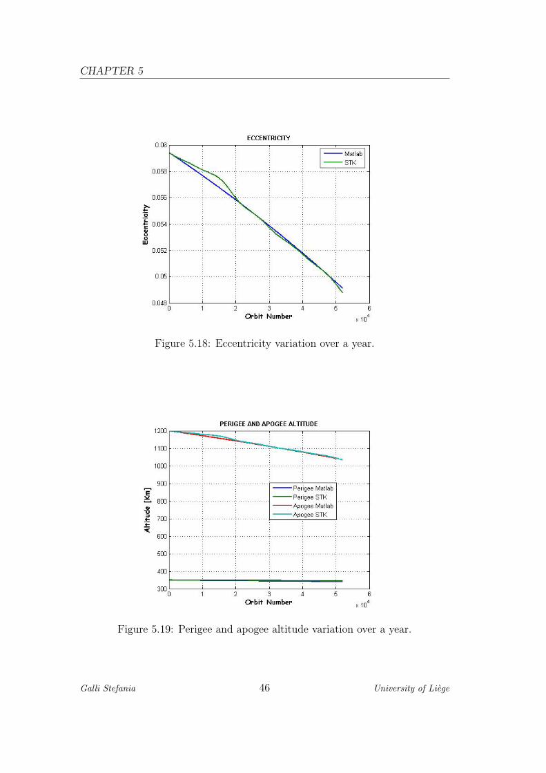
Figure 5.19: Perigee and apogee altitude variation over a year.
Galli Stefania 46 University of Liege
CHAPTER 5. MISSION ANALYSIS
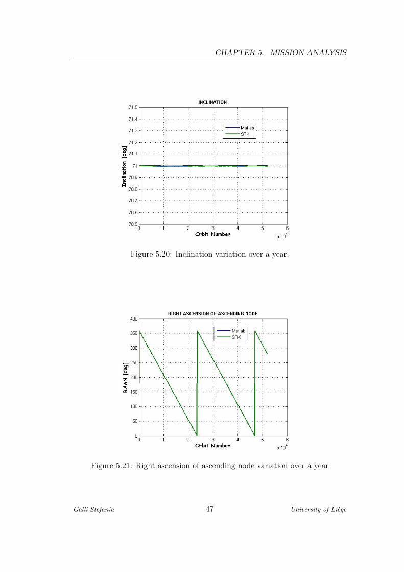
Figure 5.20: Inclination variation over a year.
Figure 5.21: Right ascension of ascending node variation over a year
Galli Stefania 47 University of Liege
CHAPTER 5
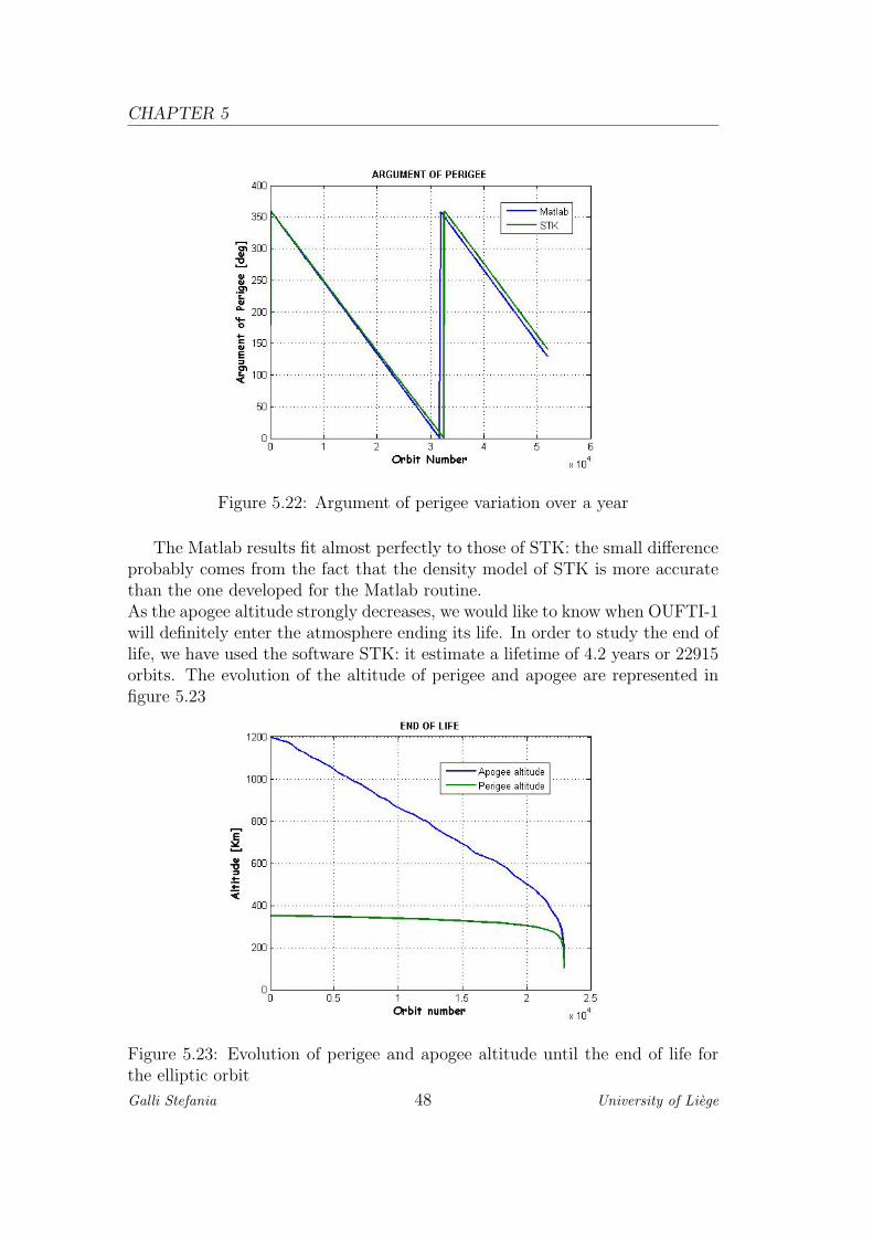
Figure 5.22: Argument of perigee variation over a year
The Matlab results fit almost perfectly to those of STK: the small differenceprobably comes from the fact that the density model of STK is more accuratethan the one developed for the Matlab routine.As the apogee altitude strongly decreases, we would like to know when OUFTI-1will definitely enter the atmosphere ending its life. In order to study the end oflife, we have used the software STK: it estimate a lifetime of 4.2 years or 22915orbits. The evolution of the altitude of perigee and apogee are represented infigure 5.23
Figure 5.23: Evolution of perigee and apogee altitude until the end of life forthe elliptic orbit
Galli Stefania 48 University of Liege

CHAPTER 5. MISSION ANALYSIS
A four year lifetime is probably much more than operating lifetime of ourD-STAR payload. In fact, as explained in paragraph 5.7, the radiation envi-ronment in the foreseen orbit is pretty hard and we still do not know neitherthe total radiation dose that can be tolerated nor the frequency of Single EventPhenomena (SEP) in that orbit for a given electronic part.Concerning the circular orbit at 350 Km altitude, the lifetime with the sameconditions (cD = 2.2 and cross-sectional area equivalent to a face’s surface) wehave a lifetime of 54 days (867 orbits) and the evolution of the perigee andapogee altitude is represented in figure 5.24
Figure 5.24: Evolution of perigee and apogee altitude until the end of life forthe circular orbit
Galli Stefania 49 University of Liege

CHAPTER 5
5.4 The launch window
The launch window represents the time gap useful to place the satellite in apredetermined orbit from a specific launch site. As the orbital plane is fixed inthe inertial space, the exact launch instant is the time when the launch site onthe surface of the earth rotates through the orbital plane.The launch is possible only if the latitude of the launch site is smaller than theorbit inclination or equal to it: here comes the importance of having a spaceportas near as possible to the equatorial line.The time to launch depends on the right ascension of ascending node and onthe inclination required.In the OUFTI-1 case, as it will be secondary payload on the launcher, we cannotchoose any of these parameters and therefore we cannot determine the launchwindows.
5.5 Earth coverage
Earth coverage refers to the surface that a spacecraft instrument or antenna cansee at one instant or over an extended period. The leading parameters are thecovered area and the rate at which new land comes into view as the spacecraftmoves. We can so identify four key parameters:
• Footprint Area also called instantaneous Field Of View area(FOV): areathat an instrument can see at any instant
• Instantaneous Access Area (IAA): all the area that an instrument couldpotentially see at any instant if it were scanned through its normal rangeof orientations
• Area Coverage Rate (ACR): the rate at which the instrument is sensingor accessing new land
• Area Access Rate (AAR): the rate at which new land is coming into thespacecraft’s access area
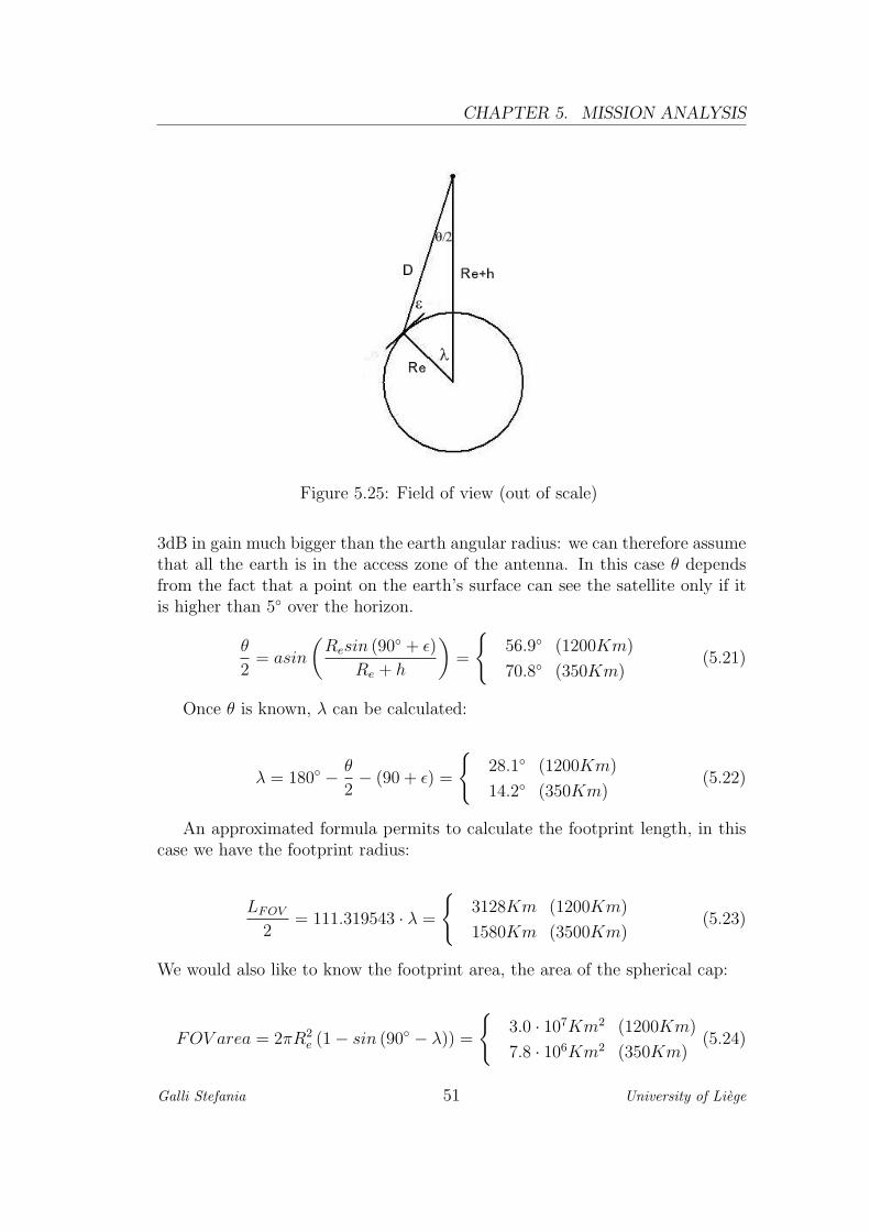
For an omnidirectional antenna, the footprint corresponds to the access area,as well the coverage rate to the access rate: for OUFTI-1 we need therefore tocalculate only two parameters.We consider a minimal elevation of the spacecraft over the horizon of ε = 5 andwe proceed to the determination of the field of view and of the area coveragerate. The notations are indicated in figure 5.25
The first step is to find out the angle θ: for a directional antenna or anoptical payload it represents the beam width and is therefore imposed. In caseof omnidirectional antenna, the directivity diagram has an angle with a loss of
Galli Stefania 50 University of Liege
CHAPTER 5. MISSION ANALYSIS
Figure 5.25: Field of view (out of scale)
3dB in gain much bigger than the earth angular radius: we can therefore assumethat all the earth is in the access zone of the antenna. In this case θ dependsfrom the fact that a point on the earth’s surface can see the satellite only if itis higher than 5 over the horizon.
θ
2= asin
(Resin (90 + ε)
Re + h
)=
56.9 (1200Km)
70.8 (350Km)(5.21)
Once θ is known, λ can be calculated:
λ = 180 − θ
2− (90 + ε) =
28.1 (1200Km)
14.2 (350Km)(5.22)
An approximated formula permits to calculate the footprint length, in thiscase we have the footprint radius:
LFOV
2= 111.319543 · λ =
3128Km (1200Km)
1580Km (3500Km)(5.23)
We would also like to know the footprint area, the area of the spherical cap:
FOV area = 2πR2e (1− sin (90 − λ)) =
3.0 · 107Km2 (1200Km)
7.8 · 106Km2 (350Km)(5.24)
Galli Stefania 51 University of Liege
CHAPTER 5
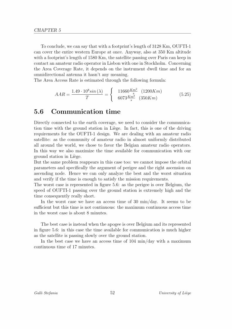
To conclude, we can say that with a footprint’s length of 3128 Km, OUFTI-1can cover the entire western Europe at once. Anyway, also at 350 Km altitudewith a footprint’s length of 1580 Km, the satellite passing over Paris can keep incontact an amateur radio operator in Lisbon with one in Stockholm. Concerningthe Area Coverage Rate, it depends on the instrument dwell time and for anomnidirectional antenna it hasn’t any meaning.The Area Access Rate is estimated through the following formula:
AAR =1.49 · 108sin (λ)
T=
11660Km2
s(1200Km)
6073Km2
s(350Km)
(5.25)
5.6 Communication time
Directly connected to the earth coverage, we need to consider the communica-tion time with the ground station in Liege. In fact, this is one of the drivingrequirements for the OUFTI-1 design. We are dealing with an amateur radiosatellite: as the community of amateur radio in almost uniformly distributedall around the world, we chose to favor the Belgian amateur radio operators.In this way we also maximize the time available for communication with ourground station in Liege.But the same problem reappears in this case too: we cannot impose the orbitalparameters and specifically the argument of perigee and the right ascension onascending node. Hence we can only analyze the best and the worst situationand verify if the time is enough to satisfy the mission requirements.The worst case is represented in figure 5.6: as the perigee is over Belgium, thespeed of OUFTI-1 passing over the ground station is extremely high and thetime consequently really short.
In the worst case we have an access time of 30 min/day. It seems to besufficient but this time is not continuous: the maximum continuous access timein the worst case is about 8 minutes.
The best case is instead when the apogee is over Belgium and its representedin figure 5.6: in this case the time available for communication is much higheras the satellite is passing slowly over the ground station.
In the best case we have an access time of 104 min/day with a maximumcontinuous time of 17 minutes.
Galli Stefania 52 University of Liege

CHAPTER 5. MISSION ANALYSIS
Figure 5.26: Worst case for communication: the white line represents thesatelite’s access to the ground station
Figure 5.27: Best case for communication: the white line represents the satelite’saccess to the ground station
Galli Stefania 53 University of Liege
CHAPTER 5
5.7 The radiation environment
The trajectory of charged particles of solar wind, electrons and protons, is mod-ified by the interaction with the earth magnetic field: they remain trapped intothe so-called radiations belts, or Van-Allen belts. They are two belts where theradiation environment is therefore extremely hard and the spacecrafts passingthrough them needs to be protected. We can in fact identify two different belts:
• the inner belt extending approximately between 1,000 and 15,000 Km. Itcontains high concentrations of energetic protons with energies exceeding100 MeV and electrons in the range of hundreds of kiloelectronvolts
• the outer belt extending till 50,000 Km. It contains mainly energeticelectrons.
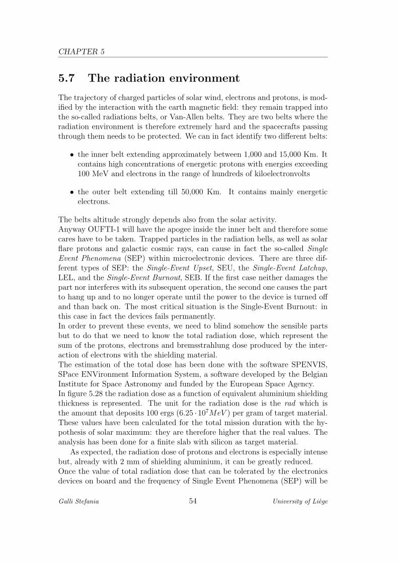
The belts altitude strongly depends also from the solar activity.Anyway OUFTI-1 will have the apogee inside the inner belt and therefore somecares have to be taken. Trapped particles in the radiation bells, as well as solarflare protons and galactic cosmic rays, can cause in fact the so-called SingleEvent Phenomena (SEP) within microelectronic devices. There are three dif-ferent types of SEP: the Single-Event Upset, SEU, the Single-Event Latchup,LEL, and the Single-Event Burnout, SEB. If the first case neither damages thepart nor interferes with its subsequent operation, the second one causes the partto hang up and to no longer operate until the power to the device is turned offand than back on. The most critical situation is the Single-Event Burnout: inthis case in fact the devices fails permanently.In order to prevent these events, we need to blind somehow the sensible partsbut to do that we need to know the total radiation dose, which represent thesum of the protons, electrons and bremsstrahlung dose produced by the inter-action of electrons with the shielding material.The estimation of the total dose has been done with the software SPENVIS,SPace ENVironment Information System, a software developed by the BelgianInstitute for Space Astronomy and funded by the European Space Agency.In figure 5.28 the radiation dose as a function of equivalent aluminium shieldingthickness is represented. The unit for the radiation dose is the rad which isthe amount that deposits 100 ergs (6.25 · 107MeV ) per gram of target material.These values have been calculated for the total mission duration with the hy-pothesis of solar maximum: they are therefore higher that the real values. Theanalysis has been done for a finite slab with silicon as target material.
As expected, the radiation dose of protons and electrons is especially intensebut, already with 2 mm of shielding aluminium, it can be greatly reduced.Once the value of total radiation dose that can be tolerated by the electronicsdevices on board and the frequency of Single Event Phenomena (SEP) will be
Galli Stefania 54 University of Liege
CHAPTER 5. MISSION ANALYSIS
Figure 5.28: Radiation dose for the OUFTI-1 elliptical orbit
known, a suitable shielding protection will be added.
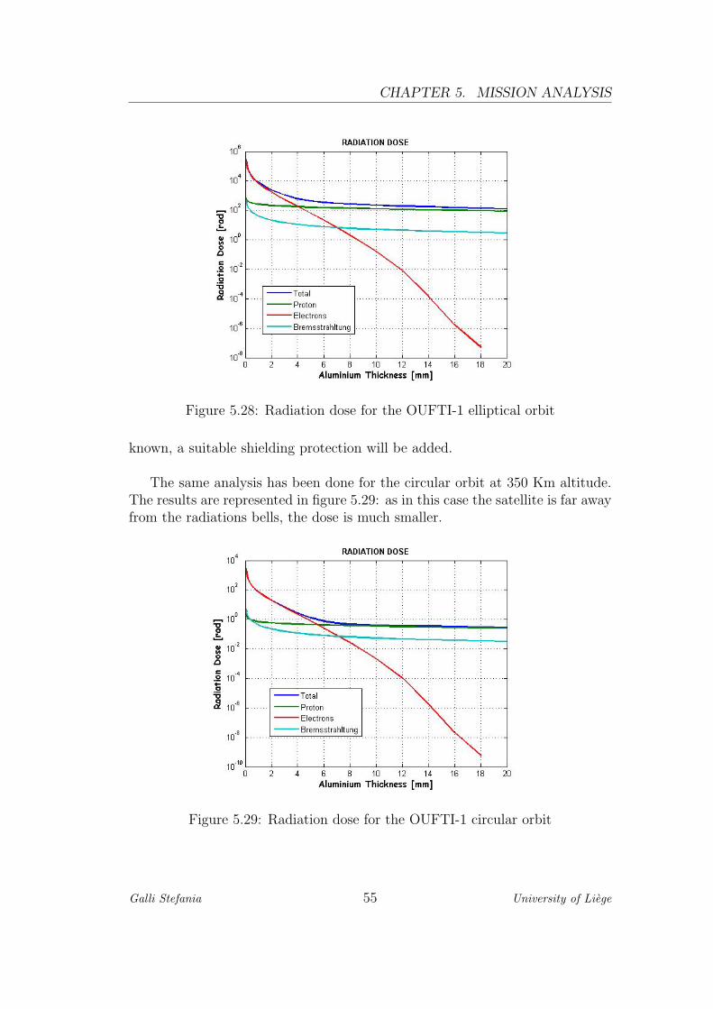
The same analysis has been done for the circular orbit at 350 Km altitude.The results are represented in figure 5.29: as in this case the satellite is far awayfrom the radiations bells, the dose is much smaller.
Figure 5.29: Radiation dose for the OUFTI-1 circular orbit
Galli Stefania 55 University of Liege

CHAPTER
6
STRUCTURE AND DEPLOYMENT
A CubeSat is a 10 cm cube with a mass up to 1 Kg: the structure’s shape iscompulsory and its mass has to be reduced at most. Furthermore, the OUFTI-1schedule is really challenging as the foreseen development time varies betweentwo and two and an half year. For these reasons, we chose to buy an off the shelfstructure. If on the one hand developing our own structure would have helpedin reaching the educational goal which characterized the project, on the otherhand it would have required a great amount of time and resources not availableat the moment and the result would have probably been less successful.As mentioned in paragraph 4.1, being a CubeSat impose some precise char-acteristics ( for more details see [AD4]). Furthermore, the European SpaceAgency add in its Call for proposal [RD2] a precise requirements: two separa-tion switches are compulsory on Vega.There are actually on the market two CubeSat structure developers: Pumpkinand ISIS. Both the two structures have their advantages and drawbacks thatwill be exposed in the following paragraph. After an accurate analysis we chosethe structure of Pumpkin as it better fits our requirements not only in terms ofstructure performances but also in terms of provided services.Concerning the antennas deployment system, they have to be folded duringlaunch and deployed once in orbit. To this end, they will be wrapped aroundcontact points and maintained in this configuration using the deployment mech-anism.
57
CHAPTER 6
6.1 Pumpkin structure
The structure developed by Pumpkin.Inc (San Francisco,CA,USA) is the mainpart of the so-called CubeSat-Kit. They offer in fact a wide range of productsfor CubeSat from hardware to software. At the moment, two of this structuresare flying on the CubeSats Libertad-1 (University Sergio Arboleda, Bogota,Colombia) and Delfi-C3 (TU Delft, The Netherlands). Concerning the last one,it’s a 3-Unit structure.The base configuration is composed by:
- Flight Model
- FM340 Flight Module
- Salvo Software and libraries
Furthermore a development board to test the CubeSat, a rechargeable elec-trical power system and an attitude determination and control system based onreactions wheels, torque coil dampers and magnetometers are available.
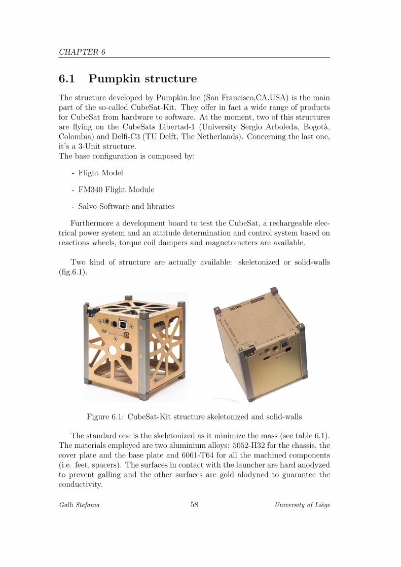
Two kind of structure are actually available: skeletonized or solid-walls(fig.6.1).
Figure 6.1: CubeSat-Kit structure skeletonized and solid-walls
The standard one is the skeletonized as it minimize the mass (see table 6.1).The materials employed are two aluminium alloys: 5052-H32 for the chassis, thecover plate and the base plate and 6061-T64 for all the machined components(i.e. feet, spacers). The surfaces in contact with the launcher are hard anodyzedto prevent galling and the other surfaces are gold alodyned to guarantee theconductivity.
Galli Stefania 58 University of Liege

CHAPTER 6. STRUCTURE AND DEPLOYMENT
All the systems have an operating temperature between -40C and +85C.The mass balance is reported in the following table:
Table 6.1: CubeSat Kit mass
Skeletonized Mass [g] Solid-Walls Mass [g]Cover plate assembly 37 49Base plate assembly 50 62
Main structure 71 132Chassis screws (x4) 2 2
Total structure 166 251Flight module 50 50
Total 216 301
The skeletonized structure results much lighter than the solid-walls one.Even if the mass balance won’t be the most critical problem for OUFTI-1 be-cause there won’t be any added payload and we are not planning to use anyattitude control, we chose the skeletonized structure. In fact, one of the goals ofthe LEODIUM project is the development of a space platform that can be useby the future CubeSats for scientific experiments: we have to make it as lighteras possible in order to have a greater mass available for payloads and attitudecontrol in the next missions, even if it wouldn’t be necessary for OUFTI-1.The main advantages of this structure is that we are sure of its reliability astwo CubeSats are already flying with it: this is the key feature that make uschoose the CubeSat-Kit. The D-STAR system into space already represents infact a challenging technology demonstration, even if we haven’t any evidencethat it won’t correctly works: adding a possible structure failure to the alreadyexisting risks seemed us too much.Certainly some budget considerations have been done too, but they have neverbeen the driving requirements.
6.2 ISIS structure
Since one and an half year, ISIS, Innovative Solution In Space (Delft, AL, TheNetherlands), has developed a CubeSat structure based on the experience gainedwith the project of Delfi-C3. They also have some other products for CubeSatsand more in general for miniaturized satellites, as antennas and ground stationand they provide a launch service.The structure is entirely made of an aluminium alloy 6061-T6 with the side-frames black hard anodised and the ribs and shear-panels black alodyned.
Galli Stefania 59 University of Liege
CHAPTER 6
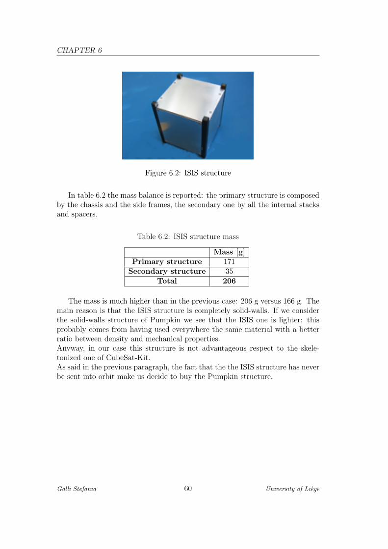
Figure 6.2: ISIS structure
In table 6.2 the mass balance is reported: the primary structure is composedby the chassis and the side frames, the secondary one by all the internal stacksand spacers.
Table 6.2: ISIS structure mass
Mass [g]Primary structure 171
Secondary structure 35Total 206
The mass is much higher than in the previous case: 206 g versus 166 g. Themain reason is that the ISIS structure is completely solid-walls. If we considerthe solid-walls structure of Pumpkin we see that the ISIS one is lighter: thisprobably comes from having used everywhere the same material with a betterratio between density and mechanical properties.Anyway, in our case this structure is not advantageous respect to the skele-tonized one of CubeSat-Kit.As said in the previous paragraph, the fact that the the ISIS structure has neverbe sent into orbit make us decide to buy the Pumpkin structure.
Galli Stefania 60 University of Liege
CHAPTER 6. STRUCTURE AND DEPLOYMENT
6.3 Deployment System
The deployment system is designed to provide a standard secondary payloadinterface between the CubeSats and the launch vehicle. Its key features are, onthe one hand, to protect the launch vehicle and its main passenger from anymechanical, electrical or electromagnetic interference from the CubeSats in theevent of a catastrophic picosatellite failure and, on the other hand, to releasethe CubeSats with a minimum spin and without any collision.The fact that the structure for a CubeSat is fixed allows the development of stan-dard deployment systems, usually called Picosatellite Orbital Deployer (POD).Currently there are four different deployment system:
• P-POD: Poly-Picosatellite Orbital Deployer. Developed by the StanfordUniversity (Stanford, CA, USA) and the California Polytechnic Institute(San Luis Obispo, CA, USA), it holds three single CubeSats stacked ontop on each other
• T-POD: Tokyo-Picosatellite Orbital Deployer. Developed by the Techni-cal University of Tokyo (Japan), it holds a single CubeSat
• X-POD: eXperimental-Push Out Deployer. Developed by the Space FlightLaboratory (SFL) of the University of Toronto Institute of AeroSpace(UTIAS) (Canada), it’a custom, independent separation system for threeCubeSats and can be tailored for satellites of different size
• SPL: Single-picosatellite Launcher. Developed by Astrofein (Berlin, Ger-many) it’a a custom deployment system for a single CubeSat
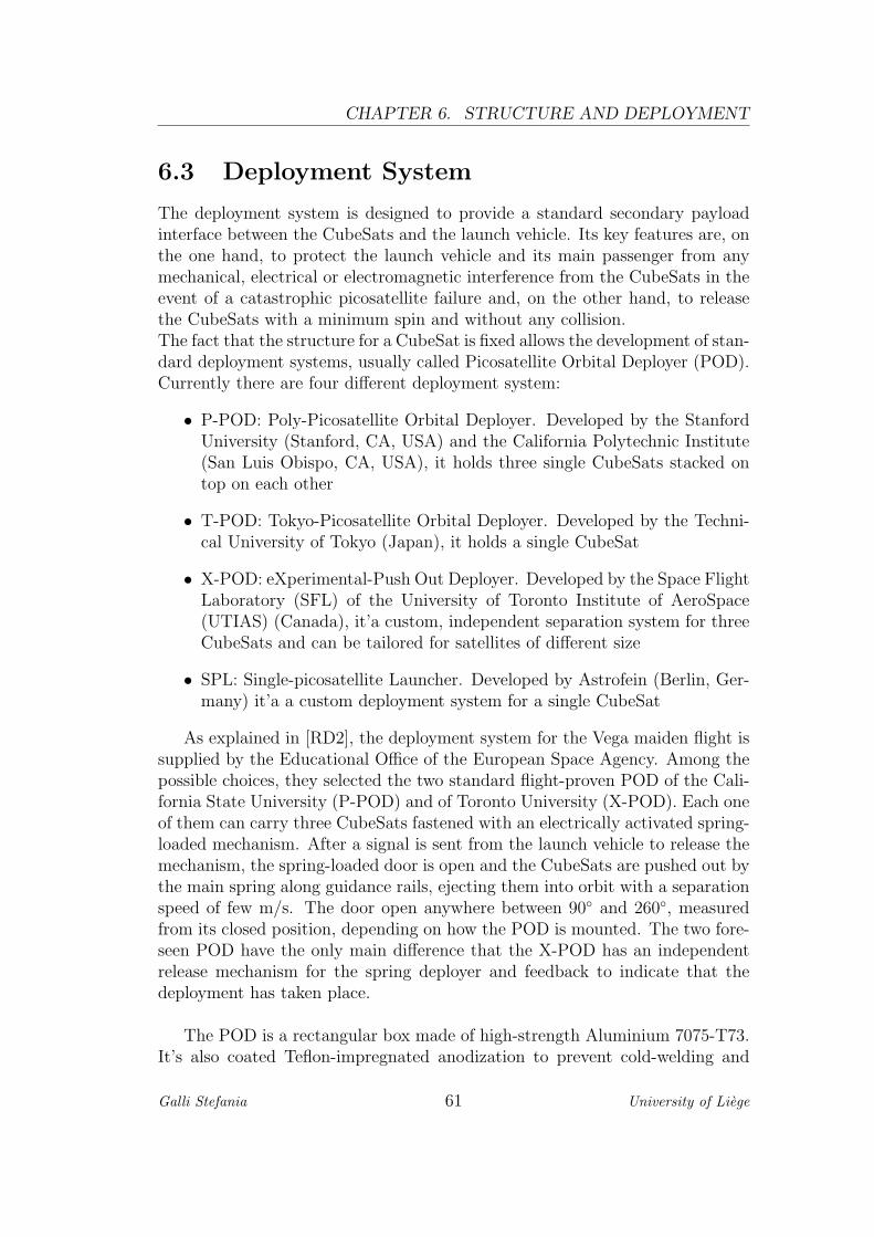
As explained in [RD2], the deployment system for the Vega maiden flight issupplied by the Educational Office of the European Space Agency. Among thepossible choices, they selected the two standard flight-proven POD of the Cali-fornia State University (P-POD) and of Toronto University (X-POD). Each oneof them can carry three CubeSats fastened with an electrically activated spring-loaded mechanism. After a signal is sent from the launch vehicle to release themechanism, the spring-loaded door is open and the CubeSats are pushed out bythe main spring along guidance rails, ejecting them into orbit with a separationspeed of few m/s. The door open anywhere between 90 and 260, measuredfrom its closed position, depending on how the POD is mounted. The two fore-seen POD have the only main difference that the X-POD has an independentrelease mechanism for the spring deployer and feedback to indicate that thedeployment has taken place.
The POD is a rectangular box made of high-strength Aluminium 7075-T73.It’s also coated Teflon-impregnated anodization to prevent cold-welding and
Galli Stefania 61 University of Liege
CHAPTER 6
Figure 6.3: P-POD: deployment system for three CubeSats
to provide a smooth guiding surface for the CubeSats during deployment. Adeployment sensor send telemetry data to the launcher: the switch is wired asa normally closed circuit and, when the door is open, the circuit opens. Thisguarantees that the door remains close until the CubeSats are deployed.Currently negotiations are going on between the Educational Office and thePOD suppliers: the final choice has’t been communicated yet but this doesn’tchange anything in the CubeSat development as both meet the same standard.
Galli Stefania 62 University of Liege
CHAPTER
7
ATTITUDE CONTROL SYSTEM
The Attitude Control System (ACS) stabilizes the spacecraft and orients it indesired directions despite to the external disturbing forces acting on it. Ac-tually, it’s part of a more complex system: the Attitude Determination andControl System (ADCS) but, in the case of OUFTI-1, speaking about attitudedetermination is inappropriate as it won’t be on board.An ADCS needs in fact sensors and actuator with the consequent mass andpower needed: this is often incompatible with a CubeSat.The incompatibility with OUFTI-1 doesn’t come much from the mass require-ment as we expect to fulfill it but from the power. As explained in chapter 10,the power produced in orbit is low because of the limited solar arrays surfaceand just enough to guarantee a good communication when the satellite is atthe apogee. Furthermore, we intend to provide OUFTI-1 with omni-directionalantennas: in this context, it does not need a priori to point in a specific di-rection and may gently tumble about all three axes. Therefore we opt for twopossible solutions: not having any kind of ACS or have a totally passive ACSwith the goal of slowing down its rotation rate due to disturbing torques and ofguaranteeing an acceptable equilibrium position.
63
CHAPTER 7
7.1 Inertia properties
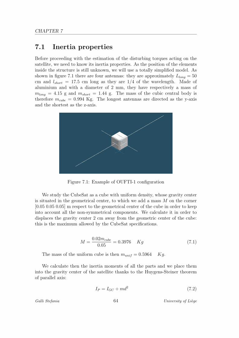
Before proceeding with the estimation of the disturbing torques acting on thesatellite, we need to know its inertia properties. As the position of the elementsinside the structure is still unknown, we will use a totally simplified model. Asshown in figure 7.1 there are four antennas: they are approximately Llong = 50cm and lshort = 17.5 cm long as they are 1/4 of the wavelength. Made ofaluminium and with a diameter of 2 mm, they have respectively a mass ofmlong = 4.15 g and mshort = 1.44 g. The mass of the cubic central body istherefore mcube = 0.994 Kg. The longest antennas are directed as the y-axisand the shortest as the z-axis.
Figure 7.1: Example of OUFTI-1 configuration
We study the CubeSat as a cube with uniform density, whose gravity centeris situated in the geometrical center, to which we add a mass M on the corner[0.05 0.05 0.05] m respect to the geometrical center of the cube in order to keepinto account all the non-symmetrical components. We calculate it in order todisplaces the gravity center 2 cm away from the geometric center of the cube:this is the maximum allowed by the CubeSat specifications.
M =0.02mcube
0.05= 0.3976 Kg (7.1)
The mass of the uniform cube is then munif = 0.5964 Kg.
We calculate then the inertia moments of all the parts and we place theminto the gravity center of the satellite thanks to the Huygens-Steiner theoremof parallel axis:
IP = IGC + md2 (7.2)
Galli Stefania 64 University of Liege
CHAPTER 7. ATTITUDE CONTROL SYSTEM
where IGC and IP are respectively the inertia moment respect to an axispassing through the gravity center and the one respect to an axis parallel to theprevious one and passing through the point P; d id the distance between thetwo axis.
So the moments of inertia of the cube of uniform density respect to thegravity center of the satellite are:
Ix,cube = Iy,cube = Iz,cube =munif l
2
6+ munif
(0.032 + 0.032
)= 1.47 · 10−3 Kgm2(7.3)
Then, the moment of inertia of the mass M respect to the gravity centerare:
Ix,M = Iy,M = Iz,M = M(0.032 + 0.032
)= 7.16 · 10−4 Kgm2 (7.4)
If we call 3 the longitudinal axis of each antenna, its moments of inertiarespect to its extremities are:
Ilong = I1,long = I2,long =mlongl
2long
3= 3.32 · 10−4 Kgm2
Ishort = I1,short = I2,short =mshortl
2short
3= 1.39 · 10−5 Kgm2
I3,long∼= I3,short
∼= 0
(7.5)
With the y-axis directed as the longer antennas and the z-axis as the shorter,we can now have the antennas moments of inertia respect to gravity center:
Ix,ant =Ilong + mlong
(0.022 + 0.033
)+ Ilong + mlong
(0.022 + 0.073
)+
+Ishort + mshort
(0.022 + 0.033
)+ Ishort + mshort
(0.022 + 0.073
)=
=7.28 · 10−4 Kgm2
Iy,ant =mlong
(0.022 + 0.023
)+ mlong
(0.022 + 0.023
)+
+Ishort + mshort
(0.022 + 0.033
)+ Ishort + mshort
(0.022 + 0.073
)=
=4.38 · 10−5 Kgm2
Iz,ant =Ilong + mlong
(0.022 + 0.033
)+ Ilong + mlong
(0.022 + 0.073
)+
+mshort
(0.022 + 0.023
)+ mshort
(0.022 + 0.023
)=
=6.93 · 10−4 Kgm2
(7.6)
Hence, the total moment of inertia are:
Galli Stefania 65 University of Liege
CHAPTER 7
Ix = Ix,cube + Ix,M + Ix,ant = 2.91 · 10−3 Kgm2
Iy = Iy,cube + Iy,M + Iy,ant = 2.23 · 10−3 Kgm2
Iz = Iz,cube + Iz,M + Iz,ant = 2.88 · 10−3 Kgm2
(7.7)
7.2 Disturbing torques
The first step to identify the most appropriate ACS is to quantify the distur-bance torques acting on the satellite. They are affected by spacecraft orienta-tion, mass properties and design symmetry. In a preliminary design phase istherefore impossible to have a precise estimation of these torques because someparameters, as the inertia moments or the center of mass position, aren’t wellknown yet . The only thing we can do is to quantify the maximal disturbancetorque that we expect to have.Once the inertia properties are known, we can proceed with the quantificationof the disturbance torques.We identify four main sources of disturbance:
• The gravity gradient : generated by the fact that the mass is not uniformlydistributed and therefore the gravity force vary depending on the position,it forces the axis of minimum inertia moment to align themself with thenadir direction:
Tgg =3µ
r3(R× IR) (7.8)
where R is the nadir direction and I the inertia matrix. If we pose θ =45 (angular displacement of the minimum inertia axis from the nadirdirection) and r =apogee radius, we are in the worst case:
TGG,max =3µ
2r3|Imax − Imin| sin (2θ) = 1.33 · 10−9 Nm (7.9)
For an inertial spacecraft it is cyclic and it depends mainly from the inertiaproperties of the vehicle and from its altitude.
• Solar radiation: generated by the solar pressure whose resultant acts overthe surface on a specific point, not coinciding with the center of mass.
TSP =Cs
c(1−R)
∑rsk ×
(nT
k S)SAk (7.10)
Galli Stefania 66 University of Liege
CHAPTER 7. ATTITUDE CONTROL SYSTEM
where Cs is the solar constant, c the speed of light, R the reflectivityfactor, rsk the vector from the center of mass to the k’th surface elementAk, nk the outward surface normal and S the unit vector from satellite tosun.We pose R = 0.6, in a simplified scalar expression and we have:
TSP,max =Cs
cA (1 + R) cos(i) (cSP − cGC) = 2.06 · 10−9 Nm (7.11)
where i = 0 is incidence angle of sun and cSP − cGC =√
0.022 + 0.022
the distance between the center of mass and the center of solar pressure,projected on the surface.It’s usually cyclic when the satellite turns around the earth or arounditself (constant only for sun-oriented vehicles) and depends mainly fromthe surface properties and from the spacecraft geometry.
• Aerodynamic drag : generated by the aerodynamic drag acting on the facein a point non coinciding with the gravity center.
TA =1
2ρv2cD
∑rsk ×
(nT
k V)
VAk (7.12)
where cD is the drag coefficient, rsk the vector from the center of mass tothe k’th surface element Ak, nk the outward surface normal, V the unitvector of velocity and V the module of the velocity vector.With cD = 2 and at the perigee we have:
TA =1
2ρv2AcD (cA − cGC) = 1.84 · 10−7 Nm (7.13)
where cA the center of aerodynamic force.Variable for inertially oriented vehicle, it depends from the altitude andon the geometry.
• Magnetic field : generated by the coupling between the earth magneticfield and the satellite residual dipole.
TM = D×B (7.14)
where B is the earth magnetic field and D the residual dipole. For themoment we are not able to estimate it.
Galli Stefania 67 University of Liege
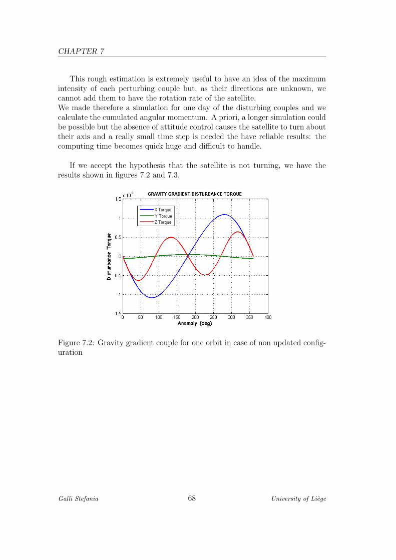
CHAPTER 7
This rough estimation is extremely useful to have an idea of the maximumintensity of each perturbing couple but, as their directions are unknown, wecannot add them to have the rotation rate of the satellite.We made therefore a simulation for one day of the disturbing couples and wecalculate the cumulated angular momentum. A priori, a longer simulation couldbe possible but the absence of attitude control causes the satellite to turn abouttheir axis and a really small time step is needed the have reliable results: thecomputing time becomes quick huge and difficult to handle.
If we accept the hypothesis that the satellite is not turning, we have theresults shown in figures 7.2 and 7.3.
Figure 7.2: Gravity gradient couple for one orbit in case of non updated config-uration
Galli Stefania 68 University of Liege
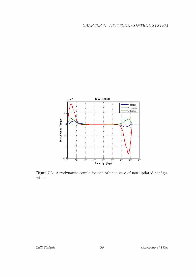
CHAPTER 7. ATTITUDE CONTROL SYSTEM
Figure 7.3: Aerodynamic couple for one orbit in case of non updated configu-ration
Galli Stefania 69 University of Liege
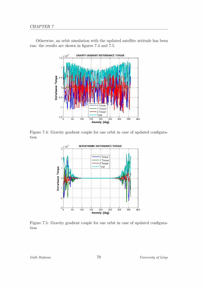
CHAPTER 7
Otherwise, an orbit simulation with the updated satellite attitude has beenrun: the results are shown in figures 7.4 and 7.5.
Figure 7.4: Gravity gradient couple for one orbit in case of updated configura-tion
Figure 7.5: Gravity gradient couple for one orbit in case of updated configura-tion
Galli Stefania 70 University of Liege
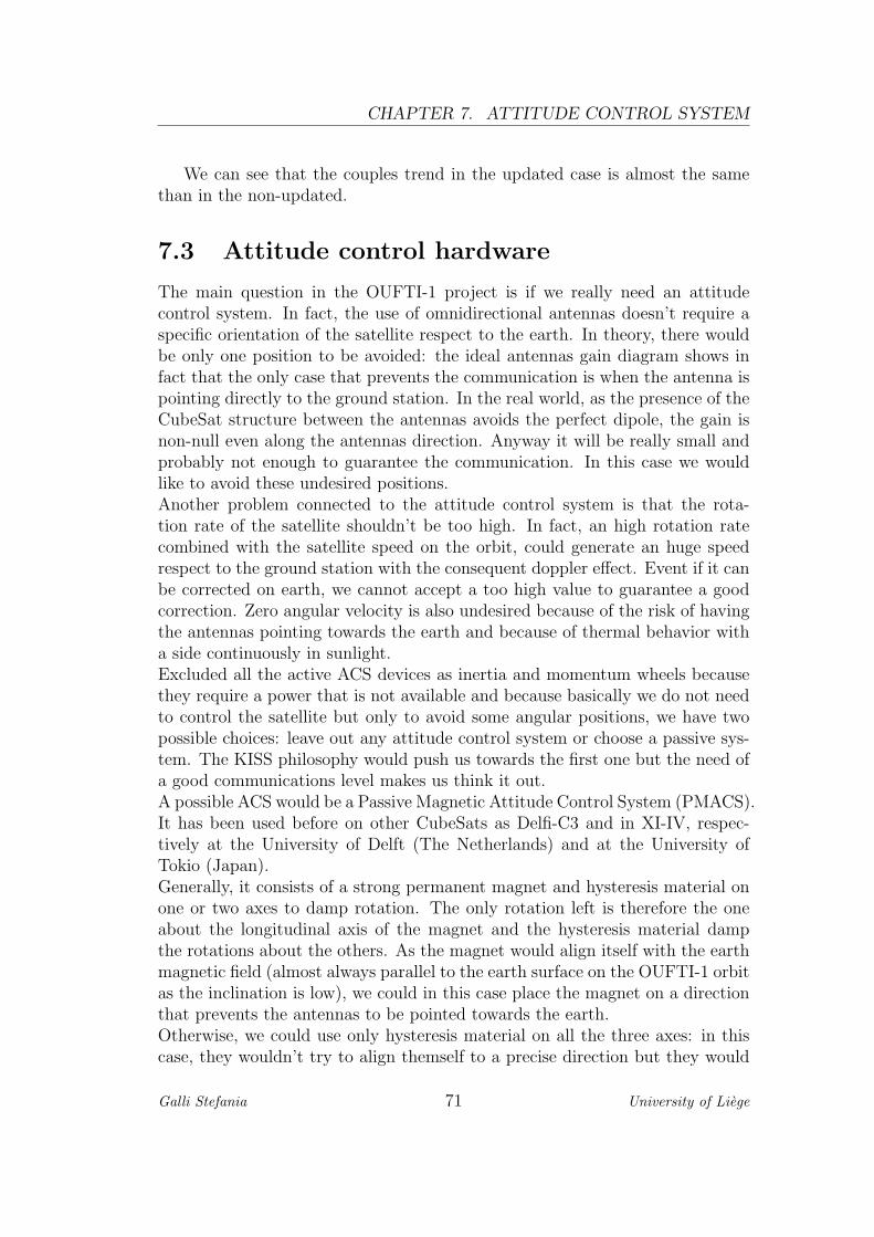
CHAPTER 7. ATTITUDE CONTROL SYSTEM
We can see that the couples trend in the updated case is almost the samethan in the non-updated.
7.3 Attitude control hardware
The main question in the OUFTI-1 project is if we really need an attitudecontrol system. In fact, the use of omnidirectional antennas doesn’t require aspecific orientation of the satellite respect to the earth. In theory, there wouldbe only one position to be avoided: the ideal antennas gain diagram shows infact that the only case that prevents the communication is when the antenna ispointing directly to the ground station. In the real world, as the presence of theCubeSat structure between the antennas avoids the perfect dipole, the gain isnon-null even along the antennas direction. Anyway it will be really small andprobably not enough to guarantee the communication. In this case we wouldlike to avoid these undesired positions.Another problem connected to the attitude control system is that the rota-tion rate of the satellite shouldn’t be too high. In fact, an high rotation ratecombined with the satellite speed on the orbit, could generate an huge speedrespect to the ground station with the consequent doppler effect. Event if it canbe corrected on earth, we cannot accept a too high value to guarantee a goodcorrection. Zero angular velocity is also undesired because of the risk of havingthe antennas pointing towards the earth and because of thermal behavior witha side continuously in sunlight.Excluded all the active ACS devices as inertia and momentum wheels becausethey require a power that is not available and because basically we do not needto control the satellite but only to avoid some angular positions, we have twopossible choices: leave out any attitude control system or choose a passive sys-tem. The KISS philosophy would push us towards the first one but the need ofa good communications level makes us think it out.A possible ACS would be a Passive Magnetic Attitude Control System (PMACS).It has been used before on other CubeSats as Delfi-C3 and in XI-IV, respec-tively at the University of Delft (The Netherlands) and at the University ofTokio (Japan).Generally, it consists of a strong permanent magnet and hysteresis material onone or two axes to damp rotation. The only rotation left is therefore the oneabout the longitudinal axis of the magnet and the hysteresis material dampthe rotations about the others. As the magnet would align itself with the earthmagnetic field (almost always parallel to the earth surface on the OUFTI-1 orbitas the inclination is low), we could in this case place the magnet on a directionthat prevents the antennas to be pointed towards the earth.Otherwise, we could use only hysteresis material on all the three axes: in thiscase, they wouldn’t try to align themself to a precise direction but they would
Galli Stefania 71 University of Liege

CHAPTER 7
only slow down the rotation rate.The two possibilities are under study and only more detailed analysis wouldallow the choice between them.
Galli Stefania 72 University of Liege
CHAPTER
8
POWER SYSTEM
The electrical power system provides, stores, distributes and controls spacecraftelectrical power.In this chapter, we will take care only of the power source: the hardware forpower control and distribution won’t be part of this work.The power source on an earth orbiting satellite is usually the sun power: throughsolar arrays we can in fact collect the sun rays and transform their energy intoelectrical power. As the performances of solar cells are subjected to degradationalong the mission, we speak about Beginning Of Life (BOL) and End of Life(EOL). As the radiation environment over the foreseen orbit is hard, the solarcells will be affected by an important degradation of their efficiency: all theanalysis will be carry out with the EOL parameters.Usually the first step is to identify the power needed in order to adapt the solararrays surface to the requirements. In the case of a CubeSat, the problem isdifferent as the surface if fixed: even if deployable orientable solar arrays areavailable, the constraints of mass and volume often hold the design back fromthese heavy and risky elements. Furthermore, OUFTI-1 need power only forthe communication system and for the on-board computer. We will thereforeproceed in the identification of the available power and then we will size theD-STAR system in order to work with it.Two scenarios are still open, depending on the final design of the communicationsystem: the payload can be on all the time or it can be switch off when it’s notused, for instance over the oceans. If the former option is the safer as the systemis never turn off and there isn’t any risk of problems in turning it on, the latterwould allow an important power saving. As we follow the KISS principle asfar as it’s possible, we would prefer to leave the payload active all the time in
73
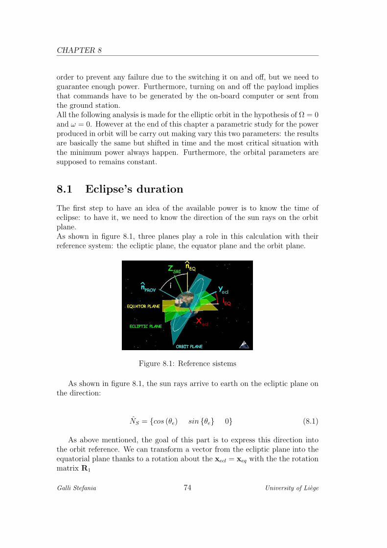
CHAPTER 8
order to prevent any failure due to the switching it on and off, but we need toguarantee enough power. Furthermore, turning on and off the payload impliesthat commands have to be generated by the on-board computer or sent fromthe ground station.All the following analysis is made for the elliptic orbit in the hypothesis of Ω = 0and ω = 0. However at the end of this chapter a parametric study for the powerproduced in orbit will be carry out making vary this two parameters: the resultsare basically the same but shifted in time and the most critical situation withthe minimum power always happen. Furthermore, the orbital parameters aresupposed to remains constant.
8.1 Eclipse’s duration
The first step to have an idea of the available power is to know the time ofeclipse: to have it, we need to know the direction of the sun rays on the orbitplane.As shown in figure 8.1, three planes play a role in this calculation with theirreference system: the ecliptic plane, the equator plane and the orbit plane.
Figure 8.1: Reference sistems
As shown in figure 8.1, the sun rays arrive to earth on the ecliptic plane onthe direction:
NS = cos (θe) sin θe 0 (8.1)
As above mentioned, the goal of this part is to express this direction intothe orbit reference. We can transform a vector from the ecliptic plane into theequatorial plane thanks to a rotation about the xecl = xeq with the the rotationmatrix R1
Galli Stefania 74 University of Liege

CHAPTER 8. POWER SYSTEM
Figure 8.2: Sun rays direction on the ecliptic plane
xeq
yeq
zeq
=
1 0 00 cos (ieq) sin (ieq)0 −sin (ieq) cos (ieq)
xecl
yecl
zecl
= R1
xecl
yecl
zecl
(8.2)
One we have our vector expressed in the equatorial plane, we pass into afirst intermediate reference by turning of the right ascension of ascending nodeΩ about the zeq = z′ axis with the rotation matrix R2:
x′
y′
z′
=
cos (Ω) sin (Ω) 0−sin (Ω) cos (Ω) 0
0 0 1
xeq
yeq
zeq
= R2
xeq
yeq
zeq
(8.3)
Then we can consider the orbit inclination i for a rotation about the x′ = x′′
axis thanks to the rotation matrix R3 and passing into a second intermediatereference:
x′′
y′′
z′′
=
1 0 00 cos (i) sin (i)0 −sin (i) cos (i)
x′
y′
z′
= R3
x′
y′
z′
(8.4)
This second reference system is on the orbit plane but the abscissas axisisn’t oriented to the perigee. We consider therefore the argument of perigee byrotating about the z′′ = zorb with the matrix R4:
xorb
yorb
zorb
=
cos (ω) sin (ω) 0−sin (ω) cos (ω) 0
0 0 1
x′′
y′′
z′′
= R4
x′′
y′′
z′′
(8.5)
Galli Stefania 75 University of Liege

CHAPTER 8
We have now the vector Ns expressed into the orbit reference:xorb
yorb
zorb
= R4R3R2R1
xecl
yecl
zecl
(8.6)
As the satellite is moving on the orbit plane, what we are interested in tocalculate the eclipses time is actually the projection of Ns on the orbit plane.As indicated in figure 8.1, we calculate the angle β that the projection of Ns
generates with the xorb:
Ns = atan
(Ns,y
Ns,x
)(8.7)
Figure 8.3: Sun rays direction projected on the orbit plane.
So far, we know the eclipse’s central angle θ∗ = 180 + β and therefore weknow the corresponding orbit radius.As the distance between earth and sun is much bigger than the earth’s radius,we can make the hypothesis that the lines determining the entrance and the exitfrom eclipses are tangent to the earth surface, as shown in figure 8.1. Hence,we have:
θout = 90 − acos
(Re
rout
)θin = 90 − acos
(Re
rin
) (8.8)
We can also exploit the relationship between radius and anomaly and wehave:
Galli Stefania 76 University of Liege
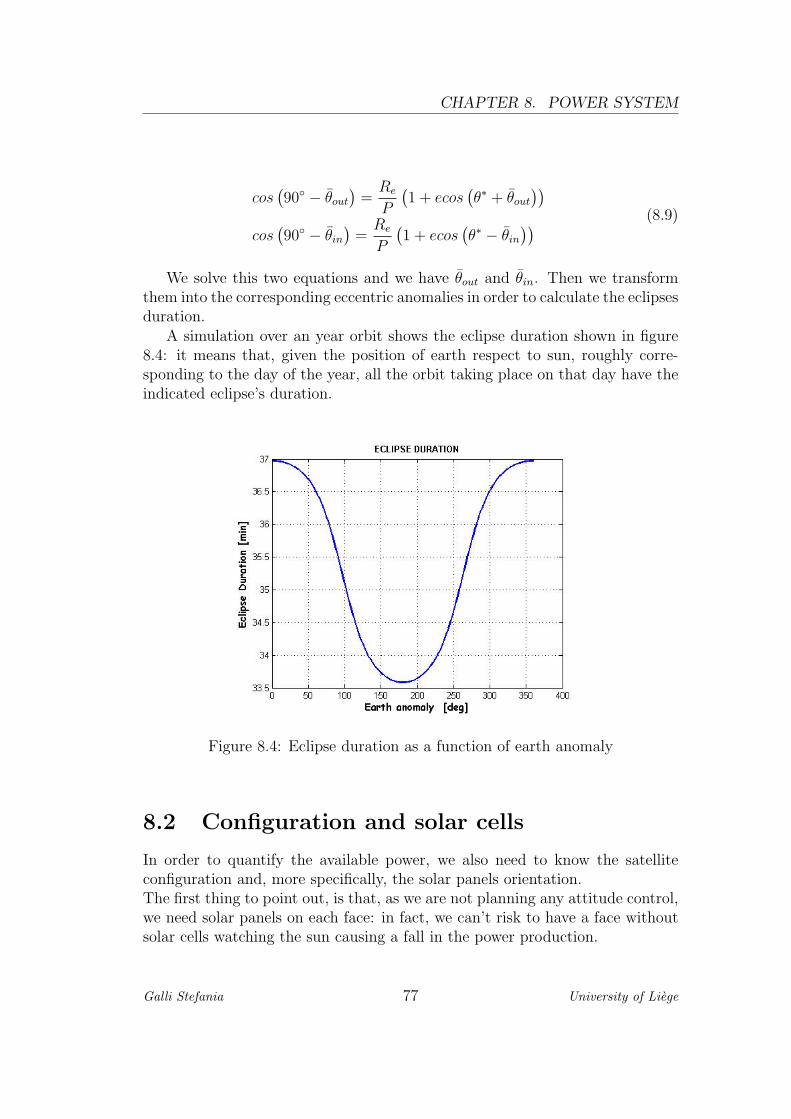
CHAPTER 8. POWER SYSTEM
cos(90 − θout
)=
Re
P
(1 + ecos
(θ∗ + θout
))cos
(90 − θin
)=
Re
P
(1 + ecos
(θ∗ − θin
)) (8.9)
We solve this two equations and we have θout and θin. Then we transformthem into the corresponding eccentric anomalies in order to calculate the eclipsesduration.
A simulation over an year orbit shows the eclipse duration shown in figure8.4: it means that, given the position of earth respect to sun, roughly corre-sponding to the day of the year, all the orbit taking place on that day have theindicated eclipse’s duration.
Figure 8.4: Eclipse duration as a function of earth anomaly
8.2 Configuration and solar cells
In order to quantify the available power, we also need to know the satelliteconfiguration and, more specifically, the solar panels orientation.The first thing to point out, is that, as we are not planning any attitude control,we need solar panels on each face: in fact, we can’t risk to have a face withoutsolar cells watching the sun causing a fall in the power production.
Galli Stefania 77 University of Liege
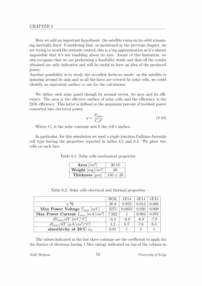
CHAPTER 8
Here we add an important hypothesis: the satellite turns on its orbit remain-ing inertially fixed. Considering that, as mentioned in the previous chapter, weare trying to avoid the attitude control, this is a big approximation as it’s almostimpossible that it’s not tumbling about its axis. Aware of this limitation, wealso recognize that we are performing a feasibility study and that all the resultsobtained are only indicative and will be useful to have an idea of the producedpower.Another possibility is to study the so-called barbecue mode: as the satellite isspinning around its axis and as all the faces are covered by solar cells, we couldidentify an equivalent surface to use for the calculation.
We define each solar panel though its normal vector, its area and its effi-ciency. The area is the effective surface of solar cells and the efficiency is theEOL efficiency. This latter is defined as the maximum percent of incident powerconverted into electrical power:
η =Pmax
CsS(8.10)
Where Cs is the solar constant and S the cell’s surface.
In particular, for this simulation we used a triple junction Gallium-Arsenidecell type having the properties reported in tables 8.1 and 8.2. We place twocells on each face.
Table 8.1: Solar cells mechanical properties
Area [cm2] 30.18Weight [mg/cm2] 86Thickness [µm] 150 ± 20
Table 8.2: Solar cells electrical and thermal properties
BOL 1E14 5E14 1E15η % 26.8 0.953 0.913 0.886
Max Power Voltage Vmax [mV ] 2275 0.0953 0.920 0.908Max Power Current Imax [mA/cm2] 7.922 1 0.993 0.976
dVmax/dT [mV/C] -6.4 -6.8 -6.8 -7.0dImax/dT [µA/cm2/C] 4.2 6.7 7.6 8.4
absorbivity at 28C α0 0.91 1 1 1
The values indicated in the last three columns are the coefficient to apply forthe fluence of electrons having 1 Mev energy indicated on top of the column in
Galli Stefania 78 University of Liege
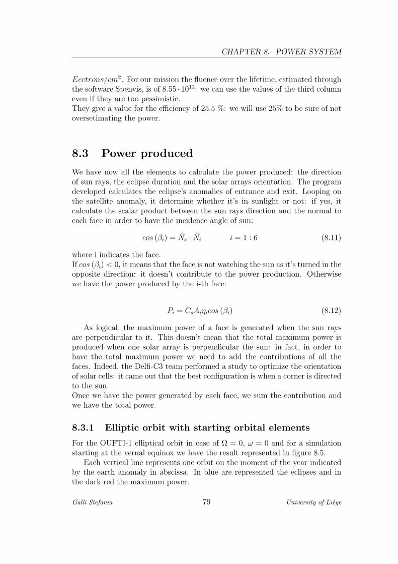
CHAPTER 8. POWER SYSTEM
Eectrons/cm2. For our mission the fluence over the lifetime, estimated throughthe software Spenvis, is of 8.55 · 1011: we can use the values of the third columneven if they are too pessimistic.They give a value for the efficiency of 25.5 %: we will use 25% to be sure of notoversetimating the power.
8.3 Power produced
We have now all the elements to calculate the power produced: the directionof sun rays, the eclipse duration and the solar arrays orientation. The programdeveloped calculates the eclipse’s anomalies of entrance and exit. Looping onthe satellite anomaly, it determine whether it’s in sunlight or not: if yes, itcalculate the scalar product between the sun rays direction and the normal toeach face in order to have the incidence angle of sun:
cos (βi) = Ns · Ni i = 1 : 6 (8.11)
where i indicates the face.If cos (βi) < 0, it means that the face is not watching the sun as it’s turned in theopposite direction: it doesn’t contribute to the power production. Otherwisewe have the power produced by the i-th face:
Pi = CsAiηicos (βi) (8.12)
As logical, the maximum power of a face is generated when the sun raysare perpendicular to it. This doesn’t mean that the total maximum power isproduced when one solar array is perpendicular the sun: in fact, in order tohave the total maximum power we need to add the contributions of all thefaces. Indeed, the Delfi-C3 team performed a study to optimize the orientationof solar cells: it came out that the best configuration is when a corner is directedto the sun.Once we have the power generated by each face, we sum the contribution andwe have the total power.
8.3.1 Elliptic orbit with starting orbital elements
For the OUFTI-1 elliptical orbit in case of Ω = 0, ω = 0 and for a simulationstarting at the vernal equinox we have the result represented in figure 8.5.
Each vertical line represents one orbit on the moment of the year indicatedby the earth anomaly in abscissa. In blue are represented the eclipses and inthe dark red the maximum power.
Galli Stefania 79 University of Liege

CHAPTER 8
Figure 8.5: Total power produced: simulation over one year orbit.
Anyway, we are more interested in the power that we can effectively use at eachtime: we calculated therefore the integrated power shown in figure 8.6. To haveit, we integrate the power over each orbit to have the total energy availableand then we divided it by the orbit duration. In this way, we know exactly thepower that we can guarantee continuously to our payload. All the losses on theelectrical power system and in the battery haven’t been taken into account yet.
Figure 8.6: Integrated power: simulation over one year orbit
We can see that, even in the worst period of the year, we can guarantee 1.3W. This is the value we will use to dimension our communication system.
Galli Stefania 80 University of Liege

CHAPTER 8. POWER SYSTEM
8.3.2 Elliptic orbit with orbital elements after one yearmission and circular orbit
As in this analysis the orbital parameters are supposed to be constant, we wouldlike to have an idea of the power available after one year mission, assuming thatthe system will be able to work till that moment. We imposed then the orbitalparameters obtained by the perturbation study:
Table 8.3: Elliptic orbit with orbital parameters after one year
Perigee altitude [Km] 341Apogee altitude [Km] 1036Semi-major axis [Km] 7067
Eccentricity 0.0491Right ascension of ascending node 279
Argument of perigee 128Inclination 71
Starting with those parameters, we have the power produces represented infigure 8.7
Figure 8.7: Total power and integrated power for the orbital parameters afterone year mission
As we can see, the difference is really small: we can therefore assume thatafter one year mission we will still have enough power.
The same analysis has been performed for the circular orbit at 350 Kmaltitude: the results are in figure 8.8
We find out that the total integrated power is lower than in the ellipticcase. Even if this lack in power could appear as a main drawback, the situation
Galli Stefania 81 University of Liege
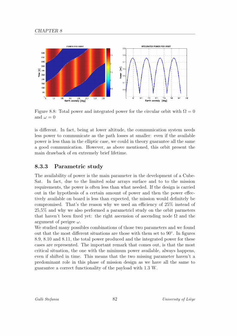
CHAPTER 8
Figure 8.8: Total power and integrated power for the circular orbit with Ω = 0and ω = 0
is different. In fact, being at lower altitude, the communication system needsless power to communicate as the path losses at smaller: even if the availablepower is less than in the elliptic case, we could in theory guarantee all the samea good communication. However, as above mentioned, this orbit present themain drawback of en extremely brief lifetime.
8.3.3 Parametric study
The availability of power is the main parameter in the development of a Cube-Sat. In fact, due to the limited solar arrays surface and to to the missionrequirements, the power is often less than what needed. If the design is carriedout in the hypothesis of a certain amount of power and then the power effec-tively available on board is less than expected, the mission would definitely becompromised. That’s the reason why we used an efficiency of 25% instead of25,5% and why we also performed a parametricl study on the orbit parmetersthat haven’t been fixed yet: the right ascension of ascending node Ω and theargument of perigee ω.We studied many possibles combinations of those two parameters and we foundout that the most different situations are those with them set to 90. In figures8.9, 8.10 and 8.11, the total power produced and the integrated power for thesecases are represented. The important remark that comes out, is that the mostcritical situation, the one with the minimum power available, always happens,even if shifted in time. This means that the two missing parameter haven’t apredominant role in this phase of mission design as we have all the same toguarantee a correct functionality of the payload with 1.3 W.
Galli Stefania 82 University of Liege
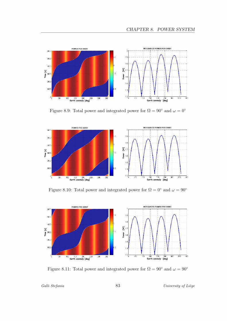
CHAPTER 8. POWER SYSTEM
Figure 8.9: Total power and integrated power for Ω = 90 and ω = 0
Figure 8.10: Total power and integrated power for Ω = 0 and ω = 90
Figure 8.11: Total power and integrated power for Ω = 90 and ω = 90
Galli Stefania 83 University of Liege

CHAPTER 8
8.4 Battery and operating modes
As above mentioned, no detailed study has been conducted over the powerhardware. Anyway, in analogy with all the other CubeSats, launched or in anadvanced design phase, we will choose a lithium-ion battery because they pro-vide more energy per kilogram than other battery types. Regarding the powerconditioning and distribution unit, a non-regulated bus possibly coupled withDC/DC converters seems the best option.The lack of active attitude control and of a specific payload simplified the identi-fications of operating modes respect to power. We have in fact only two operat-ing modes depending on the D-STAR system. We have three elements requiringpower: the D-STAR system, the on board computer and the radio beacon. Thelatter, as introduced chapter 10, is the safer communications system and needsa power much smaller than that of D-STAR.
Table 8.4: Operating modes
MODE 1 MODE 1D-STAR OFF ON
ONBOARD COMPUTER ON ONRADIO BEACON ON ON
The first mode is a kind on stand-by mode: the on board computer is on andthe radio beacon is sending the housekeeping data and receiving the commands.The second mode is the real operating mode when the D-STAR system is onand receiving and sending a amateur radio signal.
Galli Stefania 84 University of Liege

CHAPTER
9
THERMAL-CONTROL SYSTEM
The goal of thermal control is to guarantee to all the elements on board thermalconditions that allow them to reach their expected performances: each one ofthem has to be able to work when needed, during lifetime, with the requiredperformances from the beginning until the end of life.Each system has well defined temperature limits. We usually define the workingtemperature limits and the stand-by temperature limits: the former indicatesthe temperature gap where the element can work respecting the requirements,the latter the temperature gap where the elements can’t respect the specifiedrequirements but it doesn’t suffer any damage. For instance, the electronicequipments and the battery have typically as working temperature limits -20Cand +40C and as stand-by limits -40C and +60C.The thermal control can be active, semi-active or passive: we call active a systemthat needs power to work and passive a system that doesn’t. The definition ofsemi-active (or semi-passive) control system is more vague. It comes from thefact that an active system can break down, while a passive can’t, even if itcan be degradated by the external environment: we call therefore semi-active asystem that doesn’t require power but that can break down. A typical exampleare all the system with a state’s change (ex. heat pipes).On a CubeSat, because of the limited mass and power, often the only possiblechoice is a passive thermal-control system.
85

CHAPTER 9
9.1 Passive thermal-control
The thermal control of OUFTI-1 is a critical problem. In fact, as the satellite isnot-stabilized, we need to place solar cells on each face and, if we want enoughpower, we need their surface to be as big as possible: the place available forthermal control surfaces is really small. Anyway with an accurate choice of thecoating material we still can guarantee the respect of temperature limits.We chose a passive control system based on painting: we need therefore tochoose a coating and to verify that the limits are respected.The thermal equilibrium depends on the incoming and outgoing heat flux. Mak-ing it on a satellite means to consider the spacecraft, the sun, the earth and thecold space. Basing on the Wien’s law, each body radiates mainly at a wave-length which depends on its temperature: looking the temperatures of all thisbodies, we notice that the radiative exchanges are mainly at visible and infraredwavelength. Furthermore the Kirchhoff theorem says that the spectral direc-tional emissivity and absorption have the same value. Extending this theoremto the integrated absorption and emissivity, ESA and NASA adopted thereforea special convention: they call ε the absorption and emissivity factor in infraredand α the absorption and emissivity factor in visible.
α = αV IS = εV IS
ε = αIR = εIR
We will use this rule.As the incoming flux is mainly visible and the outgoing infrared, the equilibriumtemperature of a body in space depends from the ratio α
ε: the higher this ratio,
the warmer the body.Doing passive thermal control based on painting means to choose the appropri-ate color to keep the body temperature within its limits. If we have a body inspace without any kind of power production on board and we neglect the earth,the thermal balance says:
CsAα = AεσT 4 (9.1)
where Cs is the solar constant and σ = 5.67 · 10−8 Wm2K
is the Stefan-Boltzmann constant.Hence we can obtain the equilibrium temperature as:
Teq∼= 4
√Csα
σε(9.2)
In table 9.1 the value of α end ε and of the equilibrium temperature for threecolors are reported.
We see that if we want to have a cold satellite we can paint it in white, oth-erwise we can choose between black and golden, depending on the temperaturewe would like to reach.
Galli Stefania 86 University of Liege
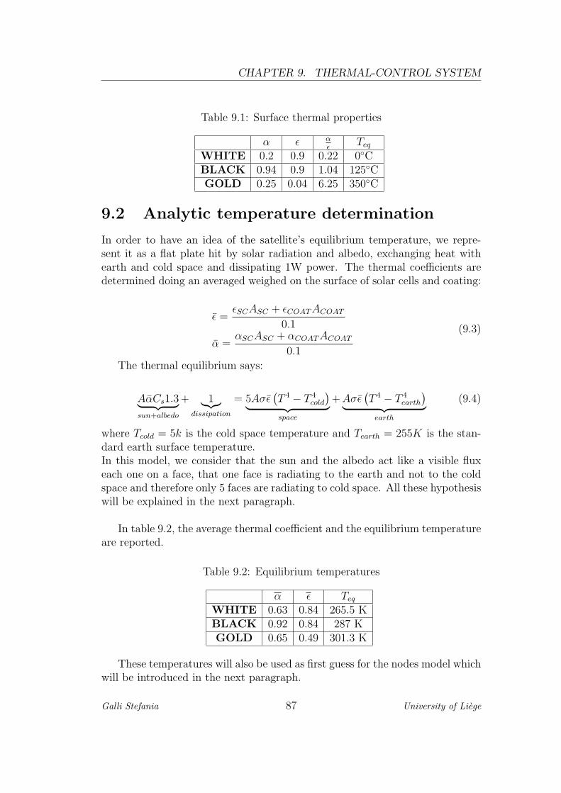
CHAPTER 9. THERMAL-CONTROL SYSTEM
Table 9.1: Surface thermal properties
α ε αε
Teq
WHITE 0.2 0.9 0.22 0CBLACK 0.94 0.9 1.04 125CGOLD 0.25 0.04 6.25 350C
9.2 Analytic temperature determination
In order to have an idea of the satellite’s equilibrium temperature, we repre-sent it as a flat plate hit by solar radiation and albedo, exchanging heat withearth and cold space and dissipating 1W power. The thermal coefficients aredetermined doing an averaged weighed on the surface of solar cells and coating:
ε =εSCASC + εCOAT ACOAT
0.1
α =αSCASC + αCOAT ACOAT
0.1
(9.3)
The thermal equilibrium says:
AαCs1.3︸ ︷︷ ︸sun+albedo
+ 1︸︷︷︸dissipation
= 5Aσε(T 4 − T 4
cold
)︸ ︷︷ ︸space
+ Aσε(T 4 − T 4
earth
)︸ ︷︷ ︸earth
(9.4)
where Tcold = 5k is the cold space temperature and Tearth = 255K is the stan-dard earth surface temperature.In this model, we consider that the sun and the albedo act like a visible fluxeach one on a face, that one face is radiating to the earth and not to the coldspace and therefore only 5 faces are radiating to cold space. All these hypothesiswill be explained in the next paragraph.
In table 9.2, the average thermal coefficient and the equilibrium temperatureare reported.
Table 9.2: Equilibrium temperatures
α ε Teq
WHITE 0.63 0.84 265.5 KBLACK 0.92 0.84 287 KGOLD 0.65 0.49 301.3 K
These temperatures will also be used as first guess for the nodes model whichwill be introduced in the next paragraph.
Galli Stefania 87 University of Liege
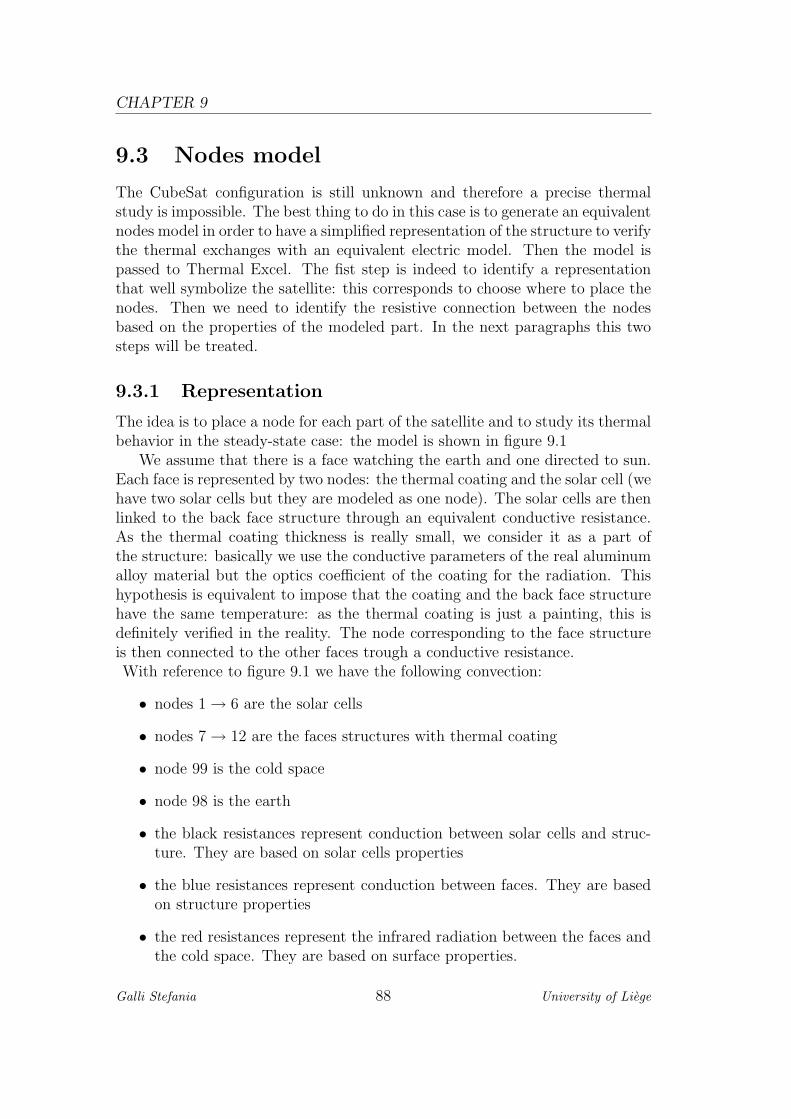
CHAPTER 9
9.3 Nodes model
The CubeSat configuration is still unknown and therefore a precise thermalstudy is impossible. The best thing to do in this case is to generate an equivalentnodes model in order to have a simplified representation of the structure to verifythe thermal exchanges with an equivalent electric model. Then the model ispassed to Thermal Excel. The fist step is indeed to identify a representationthat well symbolize the satellite: this corresponds to choose where to place thenodes. Then we need to identify the resistive connection between the nodesbased on the properties of the modeled part. In the next paragraphs this twosteps will be treated.
9.3.1 Representation
The idea is to place a node for each part of the satellite and to study its thermalbehavior in the steady-state case: the model is shown in figure 9.1
We assume that there is a face watching the earth and one directed to sun.Each face is represented by two nodes: the thermal coating and the solar cell (wehave two solar cells but they are modeled as one node). The solar cells are thenlinked to the back face structure through an equivalent conductive resistance.As the thermal coating thickness is really small, we consider it as a part ofthe structure: basically we use the conductive parameters of the real aluminumalloy material but the optics coefficient of the coating for the radiation. Thishypothesis is equivalent to impose that the coating and the back face structurehave the same temperature: as the thermal coating is just a painting, this isdefinitely verified in the reality. The node corresponding to the face structureis then connected to the other faces trough a conductive resistance.With reference to figure 9.1 we have the following convection:
• nodes 1 → 6 are the solar cells
• nodes 7 → 12 are the faces structures with thermal coating
• node 99 is the cold space
• node 98 is the earth
• the black resistances represent conduction between solar cells and struc-ture. They are based on solar cells properties
• the blue resistances represent conduction between faces. They are basedon structure properties
• the red resistances represent the infrared radiation between the faces andthe cold space. They are based on surface properties.
Galli Stefania 88 University of Liege

CHAPTER 9. THERMAL-CONTROL SYSTEM
Figure 9.1: Nodes model for thermal analysis
• the green resistances represent the infrared radiation between the facewatching the earth and the earth.
The sun light and the albedo are flux on the corresponding faces (node 2and 8 for the sun flux, nodes 5 and 11 for the albedo):
Qsun = CsαS
Qalbedo = 0.3CsαS = 0.3Qsun
(9.5)
The factor 0.3 keeps into account the average reflectivity of the earth whereseas and continents have different values: in fact the albedo is the solar visibleflux reflected by the planet.
9.3.2 Equivalent resistances
The heat transfer between two parts of a body with different temperatures T2
and T1 situated at distance L is ruled by the Fourier’s law:ρcp
∂T∂t
= ~∇~q + σ
~q = −k~∇T(9.6)
Galli Stefania 89 University of Liege
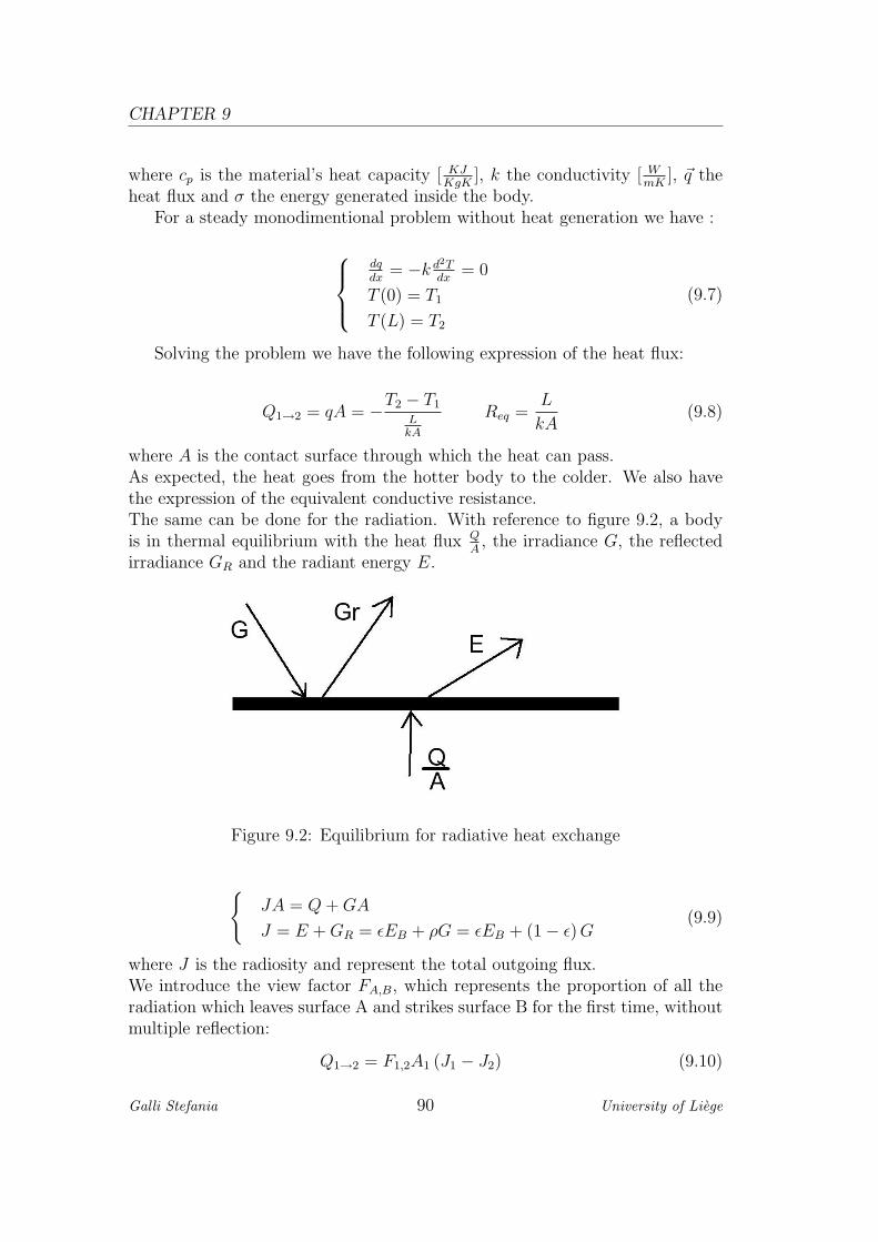
CHAPTER 9
where cp is the material’s heat capacity [ KJKgK
], k the conductivity [ WmK
], ~q theheat flux and σ the energy generated inside the body.
For a steady monodimentional problem without heat generation we have :
dqdx
= −k d2Tdx
= 0
T (0) = T1
T (L) = T2
(9.7)
Solving the problem we have the following expression of the heat flux:
Q1→2 = qA = −T2 − T1
LkA
Req =L
kA(9.8)
where A is the contact surface through which the heat can pass.As expected, the heat goes from the hotter body to the colder. We also havethe expression of the equivalent conductive resistance.The same can be done for the radiation. With reference to figure 9.2, a bodyis in thermal equilibrium with the heat flux Q
A, the irradiance G, the reflected
irradiance GR and the radiant energy E.
Figure 9.2: Equilibrium for radiative heat exchange
JA = Q + GA
J = E + GR = εEB + ρG = εEB + (1− ε) G(9.9)
where J is the radiosity and represent the total outgoing flux.We introduce the view factor FA,B, which represents the proportion of all theradiation which leaves surface A and strikes surface B for the first time, withoutmultiple reflection:
Q1→2 = F1,2A1 (J1 − J2) (9.10)
Galli Stefania 90 University of Liege
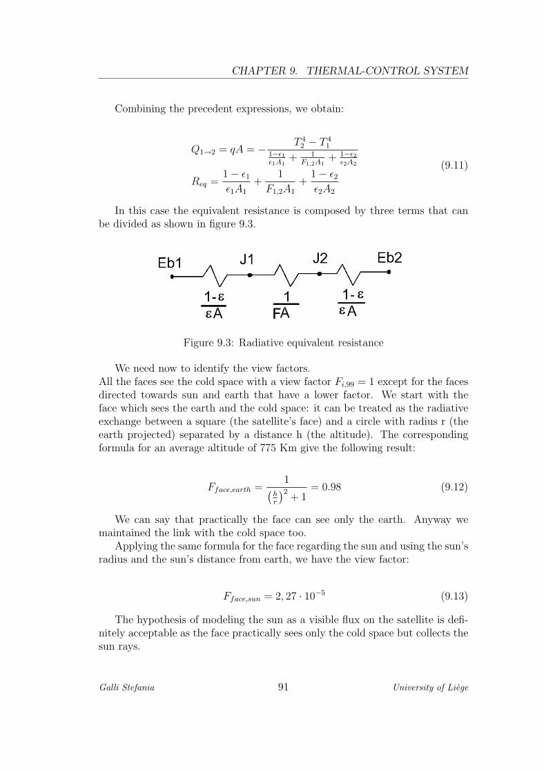
CHAPTER 9. THERMAL-CONTROL SYSTEM
Combining the precedent expressions, we obtain:
Q1→2 = qA = − T 42 − T 4
11−ε1ε1A1
+ 1F1,2A1
+ 1−ε2ε2A2
Req =1− ε1
ε1A1
+1
F1,2A1
+1− ε2
ε2A2
(9.11)
In this case the equivalent resistance is composed by three terms that canbe divided as shown in figure 9.3.
Figure 9.3: Radiative equivalent resistance
We need now to identify the view factors.All the faces see the cold space with a view factor Fi,99 = 1 except for the facesdirected towards sun and earth that have a lower factor. We start with theface which sees the earth and the cold space: it can be treated as the radiativeexchange between a square (the satellite’s face) and a circle with radius r (theearth projected) separated by a distance h (the altitude). The correspondingformula for an average altitude of 775 Km give the following result:
Fface,earth =1(
hr
)2+ 1
= 0.98 (9.12)
We can say that practically the face can see only the earth. Anyway wemaintained the link with the cold space too.
Applying the same formula for the face regarding the sun and using the sun’sradius and the sun’s distance from earth, we have the view factor:
Fface,sun = 2, 27 · 10−5 (9.13)
The hypothesis of modeling the sun as a visible flux on the satellite is defi-nitely acceptable as the face practically sees only the cold space but collects thesun rays.
Galli Stefania 91 University of Liege

CHAPTER 9
We have now all the parameters to connect the nodes: we only need thesurfaces parameters and the conductivity.If the structure’s and coating’s parameters are fixed, the solar cells opticalparameters vary as a function of the temperature.The goal of a solar cell is in fact to collect the sun’s flux and to convert it intoelectrical power: not all the energy collected becomes heat. The absorptionfactor of a solar cell varies following the relation:
α(T ) = α0 (1− η(T )) (9.14)
where α0 is the absorption at 28C and η(T ) the efficiency.This formula shows an important conclusion: higher is the efficiency, and so thepower produced, lower is the percent of collected energy converted into heat.We have so a double interest in having an efficiency as higher as possible.Then, the efficiency varies in function of temperature:
η(T ) = η0 +dη
dT(T − 28C) (9.15)
where η0 is the efficiency at 28C.As the efficiency is defined as the maximum percent of incident power con-verted into electrical energy (see formula 8.10 ), we define its derivate respectto temperature as:
dη
dT=
d
dT
(Pmax
CsS
)=
1
CsS
(Vmax
dImax
dT+ Imax
dVmax
dT
)(9.16)
Using the values indicated in table 8.2, we can calculate the absorption fac-tor of the solar cells.
Concerning the infrared emissivity ε, we need to point out that each solarcell is usually covered by a transparent tape and by a so-called cover glass whichis transparent for the visible wavelength but determine the infrared emissivity:ε is usually between 0.8 and 0.85. We used ε = 0.8.The dimension of solar cells are indicated in table 8.1.Concerning the structure, it’s an aluminium alloy with the following properties:
Table 9.3: Structure properties
Conductivity k [ WmK
] 138Thickness [mm] 1.27
Galli Stefania 92 University of Liege

CHAPTER 9. THERMAL-CONTROL SYSTEM
9.3.3 Hot and cold case
We are dealing with a simplified model: we are not expecting to have a detailedthermal description of our CubeSat. The goal of this preliminary study is toidentify the maximum and minimum temperatures reached during lifetime inorder to avoid the overpass of the imposed limits.We identify therefore three possible cases:
• the hot case: the satellite is in sunlight and the solar arrays do not produceany power but only cumulate solar heat flux. The solar flux is injected ona face and the absorption coefficient is α0 as the efficiency is null.
• the operating case: the satellite is in sunlight and the solar arrays areproviding the necessary power. The payload is on and we need to radiate0.5 W corresponding to the losses in the communication system convertedinto heat. In this case, the absorption factor of solar cells needs to beupdated as a function of the solar cell temperature
• the cold case: the satellite is in eclipse and the payload is off. In this casethe solution seems to be trivial: the equilibrium temperature is practicallythe Tcold but it doesn’t respect the reality. Furthermore in this case thehypothesis of steady-state cannot be applied integrally. We added there-fore a flux of 847W/m2, which is the solar flux weighed on the averagetime of eclipse.
For the operating case, we needed to add a worksheet to Thermal-Excel inorder to update the solar cells properties as a function their temperatures.
9.4 Thermal results for OUFTI-1
Once decided the kind of model to study and identified the material properties,we passes to the implementation into the software Thermal-Excel.As above mentioned, a starting guess temperature is demanded and for eachcase we calculated it as explained in section 9.2 respecting the characteristicsof each case.At the beginning, we had some problems as the final results depended on thestarting temperature, which is impossible for the static case. With an accuratereflection we find out the reason: the standard algorithm used by the softwarehas a really slow convergence when the number of radiative exchange is impor-tant respect to the conductive. As the criterion of convergence is the differencebetween successive temperatures, the software thought to have converged evenif it was not true. We needed therefore to strongly reduce the convergence cri-terion in order to have the good solution.
Galli Stefania 93 University of Liege
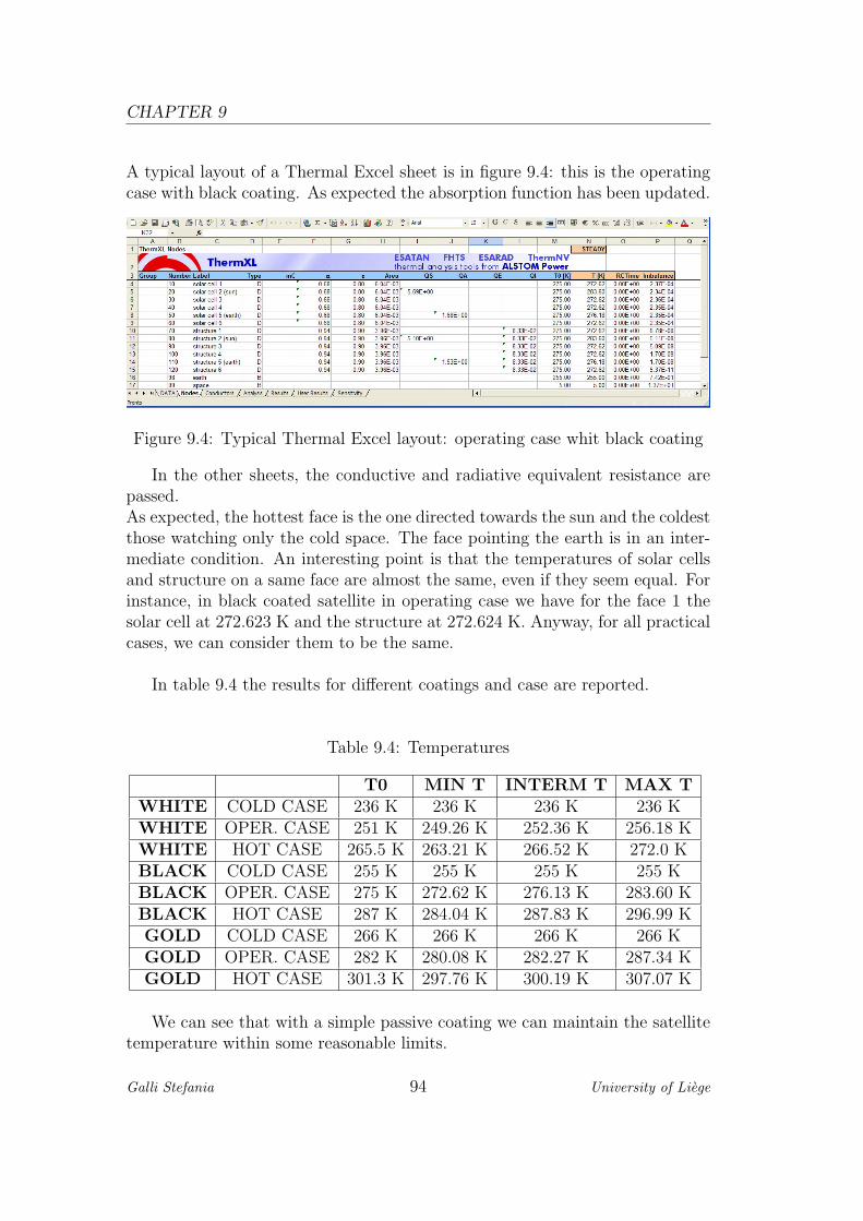
CHAPTER 9
A typical layout of a Thermal Excel sheet is in figure 9.4: this is the operatingcase with black coating. As expected the absorption function has been updated.
Figure 9.4: Typical Thermal Excel layout: operating case whit black coating
In the other sheets, the conductive and radiative equivalent resistance arepassed.As expected, the hottest face is the one directed towards the sun and the coldestthose watching only the cold space. The face pointing the earth is in an inter-mediate condition. An interesting point is that the temperatures of solar cellsand structure on a same face are almost the same, even if they seem equal. Forinstance, in black coated satellite in operating case we have for the face 1 thesolar cell at 272.623 K and the structure at 272.624 K. Anyway, for all practicalcases, we can consider them to be the same.
In table 9.4 the results for different coatings and case are reported.
Table 9.4: Temperatures
T0 MIN T INTERM T MAX TWHITE COLD CASE 236 K 236 K 236 K 236 KWHITE OPER. CASE 251 K 249.26 K 252.36 K 256.18 KWHITE HOT CASE 265.5 K 263.21 K 266.52 K 272.0 KBLACK COLD CASE 255 K 255 K 255 K 255 KBLACK OPER. CASE 275 K 272.62 K 276.13 K 283.60 KBLACK HOT CASE 287 K 284.04 K 287.83 K 296.99 KGOLD COLD CASE 266 K 266 K 266 K 266 KGOLD OPER. CASE 282 K 280.08 K 282.27 K 287.34 KGOLD HOT CASE 301.3 K 297.76 K 300.19 K 307.07 K
We can see that with a simple passive coating we can maintain the satellitetemperature within some reasonable limits.
Galli Stefania 94 University of Liege
CHAPTER 9. THERMAL-CONTROL SYSTEM
We still do not now the exact temperature limits of our D-STAR payload andtherefore we will make some comments basing on the average limits of theelectronics equipments and battery as thay are usually the most sensible tothermal gradient.We impose therefore that the working temperature has to be between 253 Kand 313 K and the stand-by temperature between 233 K and 333 K.We find out that, on the one hand, the stand-by limits are respected with all thecoating and, on the other hand, the working limits are respected only with theblack and golden coating. Furthermore, the coldest temperature for the blackcoating and the hottest temperature for the gold coating are on the borderline.For this reason, up to now we cannot chose one of this two coating as the modelis too simplified to allow a choice with so small margins. The final decision willbe taken after an accurate study based on orbit and satellite’s configurationwith the more detailed software Esatan and Esarad. Anyway, even if we don’thave a final choice, on the base of these results, we can assume that OUFTI-1will remains within the required temperature limits.
Galli Stefania 95 University of Liege

CHAPTER
10
COMMUNICATION SYSTEM
The communication system is the interface between the satellite and the earth.If in the case of OUTI-1 it also represents the payload, for the next missions ofLEODIUM Project it will be just a mean to be in contact with the spacecraft.The D-STAR system is used as main communication tool to send command,both for the satellite and for the future payloads, and to receive telemetry andpayload’s results. Given that D-STAR is an amateur-radio protocol, we planto make our CubeSat available to the ham-radio community when the radiolink is not used for command and telemetry. Furthermore, we plan to getspontaneous help from the worldwide amateur-radio community to keep an eyeon our satellite when it is not within sight of our ground station.Aware of the fact that a D-STAR has never flown into space, we cannot takefor granted that everything will go fine, especially considering the fight loadsat launch and the radiation environment in orbit. Furthermore, if somethingfails just after launch, we strongly desire to be able to assess what happenedwith the satellite. Therefore, we will place a backup command and telemetrysystem based on a CW beacon. Probably always switch on, it will be able tosend minimum housekeeping and to receive some commands.
97

CHAPTER 10
10.1 Communication hardware
The hardware for satellite D-STAR communication has never been built untilnow: it’s the main grey area of the project. In fact, a traditional D-STARground repeater is composed by a series of boxes with dimension and massdefinitely incompatible with a CubeSat: everything has to be reduced at mostand some functionalities will be cut out.We are not going to give detailed information on the subject as it’s part of another thesis on OUFTI-1 [RD5]. Anyway a brief introduction of the hardwareis almost compulsory.The system is shown in block diagram in figure 10.1
Figure 10.1: Communication system block diagram
The signal at 145 MHz frequency is received, amplified and demodulated.Voice and data stream are then separated. The low rate stream is then searchedfor command packages and, if any, they are analyzed, verified as originating fromthe Reference Control Station and then processed if suitable. In this case, down-link data are fitted with requested telemetry information. Otherwise, receivedlow rate user’s data are recombined without additional delay with the receivedvoice stream, modulated, amplified and sent back immediately via the downlinkpath at 435 MHz frequency.The mode of operation is a voice based system called DV mode: it runs at4800 bds, 0.5 GMSK modulated. It is made by 3600 bds AMBE encoded voicestream (2400 bds voice + 1200 bds FEC) and a low speed uncorrected data
Galli Stefania 98 University of Liege
CHAPTER 10. COMMUNICATION SYSTEM
stream at 1200 bds, giving about 950 bds real data throughput.Concerning the antennas, we need four different quarter-wave deployable an-tennas: two about 17 cm long for the downlink and two about 50 cm long forthe uplink. They have to be folded during launch and deployed once in orbit.To this end, they will be wrapped around contact points and maintained inthis configuration using the deployment mechanism. As mentioned in chapter7.3, they are omnidirectional and don’t require any specific orientation of thesatellite respect to the earth.More information about the communication hardware and the D-STAR protocolcan be found in [RD5].
10.2 Link budget
A link budget is the accounting of all of the gains and losses from the transmitter,through the space, to the receiver in a telecommunication system: its goal is toverify if the ratio of received energy-per-bit to noise-density Eb
N0and the signal-
to-noise ratio SN
are higher than some limit values depending on the modulationtype.As the available power is not too much, the link budget assumes a capitalrole: we need in fact to verify that the power is enough to guarantee a goodcommunication level.Starting from the available power for communication P0, through the systemefficiency η we have the power available at the transmitting antenna:
PT = ηP0 (10.1)
Then we better pass to decibel-watt instead of watt, where:
PT [dBW ] = 10log10 (PT [W ]) (10.2)
In this way, we deal with algebraic sum instead that with multiplicationsand divisions. Hereafter, if not differently specified, all the values will be indecibel-watt or decibel.
The first step is to identify the Effective Isotropic Radiated Power (EIRP)which represents the power that effectively leaves the antenna:
EIRP = PT + LT + GT (10.3)
where LT and GT are respectively losses and gains in the transmitting an-tenna.Once the electromagnetic waves have left the transmitting antenna, they need
Galli Stefania 99 University of Liege
CHAPTER 10
to reach the receiver passing through the free space. The losses on this way arecalled space loss :
Ls[W ] =RIP [W ]
EIRP [W ]=
Sλ2
4π
4πSd2=
(λ
4πd
)2
=
(c
4πdf
)2
(10.4)
where RIP is the Received Isotropic Power, λ the wavelength and S thepower per unit area at distance d.Passing in decibel, we have:
Ls[dBW ] = 20log (c)− 20log (4π)− 20log (d)− 20log (f) =
= 147.55− 20log (d)− 20log (f)(10.5)
The space loss contains the hypothesis of free-space propagation: in reality,the signal pass through the atmosphere and we would have therefore to take intoaccount the attenuation due to atmosphere and rain. As these attenuations areimportant only for high frequency wave (mainly in the SHF band and higher),they are practically are null in our case.
Once the signal is received by the receiving antenna, its gain GR should beadded.In digital communications, the received energy-per-bit Eb is equal to the receivedpower times the bit duration:
Eb = PR − 10log(R) (10.6)
where PR = RIP + GR is the received power and R the data rate.The noise spectral density, N0, can be expressed as:
N0 = 10log(k) + 10log(Ts) (10.7)
where k = 1.38 · 10−23 is the Boltzmann’s constant and Ts the system noisetemperature.Hence, the total received noise is:
N = N0 + 10log(B) (10.8)
where B is the bandwidth.
Using the above mentioned equations, we can obtain the parameters we werelooking for:
• the radio of received energy-per-bit to noise-density
Eb
N0
= EIRP + Ls + GR − 10log(k)− 10log(Ts)− 10log(R) (10.9)
Galli Stefania 100 University of Liege
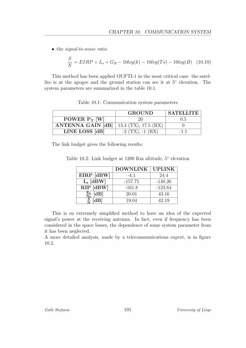
CHAPTER 10. COMMUNICATION SYSTEM
• the signal-to-noise ratio
S
N= EIRP + Ls + GR − 10log(k)− 10log(Ts)− 10log(B) (10.10)
This method has been applied OUFTI-1 in the most critical case: the satel-lite is at the apogee and the ground station can see it at 5 elevation. Thesystem parameters are summarized in the table 10.1.
Table 10.1: Communication system parameters
GROUND SATELLITEPOWER PT [W] 20 0.5
ANTENNA GAIN [dB] 13.4 (TX), 17.5 (RX) 0LINE LOSS [dB] -2 (TX), -1 (RX) -1.1
The link budget gives the following results:
Table 10.2: Link budget at 1200 Km altitude, 5 elevation
DOWNLINK UPLINKEIRP [dBW] -4.1 24.4
Ls [dBW] -157.75 -148.26RIP [dBW] -161.8 -123.84
Eb
N0[dB] 20.01 43.16
SN
[dB] 19.04 42.19
This is en extremely simplified method to have an idea of the expectedsignal’s power at the receiving antenna. In fact, even if frequency has beenconsidered in the space losses, the dependence of some system parameter fromit has been neglected.A more detailed analysis, made by a telecommunications expert, is in figure10.2.
Galli Stefania 101 University of Liege
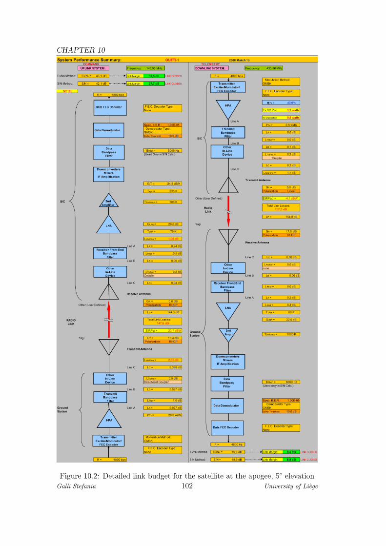
CHAPTER 10
Figure 10.2: Detailed link budget for the satellite at the apogee, 5 elevation
Galli Stefania 102 University of Liege
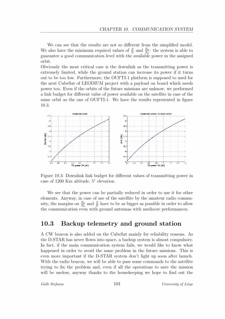
CHAPTER 10. COMMUNICATION SYSTEM
We can see that the results are not so different from the simplified model.We also have the minimum required values of S
Nand Eb
N0: the system is able to
guarantee a good communication level with the available power in the assignedorbit.Obviously the most critical case is the downlink as the transmitting power isextremely limited, while the ground station can increase its power if it turnsout to be too low. Furthermore, the OUFTI-1 platform is supposed to used forthe next CubeSat of LEODIUM project with a payload on board which needspower too. Even if the orbits of the future missions are unknow, we performeda link budget for different value of power available on the satellite in case of thesame orbit as the one of OUFTI-1. We have the results represented in figure10.3.
Figure 10.3: Downlink link budget for different values of transmitting power incase of 1200 Km altitude, 5 elevation.
We see that the power can be partially reduced in order to use it for otherelements. Anyway, in case of use of the satellite by the amateur radio commu-nity, the margins on Eb
N0and S
Nhave to be as bigger as possible in order to allow
the communication even with ground antennas with mediocre performances.
10.3 Backup telemetry and ground station
A CW beacon is also added on the CubeSat mainly for reliability reasons. Asthe D-STAR has never flown into space, a backup system is almost compulsory.In fact, if the main communication system fails, we would like to know whathappened in order to avoid the same problem in the future missions. This iseven more important if the D-STAR system don’t light up soon after launch.With the radio beacon, we will be able to pass some commands to the satellitetrying to fix the problem and, even if all the operations to save the missionwill be useless, anyway thanks to the housekeeping we hope to find out the
Galli Stefania 103 University of Liege
CHAPTER 10
failure reasons. It’s also true that, without the D-STAR system, OUFTI-1 willbe useless as inaccessible by the amateur radio community: all the tests will betherefore performed to avoid such a kind of problem.Concerning the ground station, it will be installed in the University of Liegearea. It will be a traditional tracking station for simultaneous transmission andreception on the amateur radio frequencies and it will be connected with thealready existing D-STAR repeater of the university to exploit all the systemproperties, included the connection to the internet. A backup ground stationwill also be installed in the neighborhood: it main purpose is to track othersatellites but it can be used for OUFTI-1 if needed.A possible participation of this ground station to the GENSO (Global Educa-tional Network for Satellite Operations) network is also wished.
Galli Stefania 104 University of Liege
CHAPTER
11
TESTS
The launch and space environment are extremely hard for the spacecraft: it isin fact subject to vibrations at different frequencies, vacuum and frequent ther-mal cycling. Given that, once in orbit, there is not any way to repair a damageon the satellite, we need to verify that all the components and the integratedsystem can survive to the external environment: the block of all these actionsconstitutes the test campaign. The tests usually performed on a satellite beforelaunch include mechanical test as vibrations and shocks, environmental tests asthermal vacuum and functional test as the electromagnetic compatibility. Thetests level and duration depends, on the one hand, on the test philosophy and,on the other hand, on the launcher specifications and on the space environmentexpected. We can then demonstrate some spacecraft function by testing somegroup on components: it is called verification test and typically includes theantennas and solar arrays deployment test.
105
CHAPTER 11
11.1 Test philosophy and facilities
All the elements need to be tested before being placed on board and someintegrated system test are then performed after the assembly. In the case ofOUFTI-1, the D-STAR system will undergo many functional and radiationstests before being placed on the platform for the integrated tests.The qualification and acceptance test document of a launcher, in our case Vega[AD2], gives the test intensity and duration based on the typical mission envelop.Two levels and durations are specified: the acceptance test and the qualificationtest. The acceptance spectrum envelops the expected environment and is higherthan the conducted level specified by the launch vehicle contractor to accountfor structural resonance and acoustic inputs. Respect to the qualification level,it is 3 dB lower for random vibrations and 80% of sinusoidal acceleration.Concerning the assembled satellite, the number of tests to be performed as wellas their level and duration depend on the so called test philosophy. In fact,many satellite models can be produced and tested, depending on schedule andbudget:
• structural (SM), thermal (TM) and structural and thermal (STM) models:they need to be representative of the satellite mechanical (mass, eigenfre-quencies, stiffness) and/or thermal behavior. They are tested at qualifi-cation level to verify if the design satisfy the testing requirements.
• engineering model (EM): it is composed by all the electromagnetic compo-nents and it undergoes to electromagnetic compatibility and functionalitytests.
• qualification model (QM): it is the assembled satellite and it is tested atqualification level.
• flight model (FM): it is the final model and undergoes to acceptance test.
The same kind of classification can be done for all the satellite components.In the OUFTI-1 case some models of the D-STAR board will also be tested.The spacecraft verification strategy is specified in Vega acceptance and qualifi-cation test document [AD2]. Three main types of tests are envisioned, namelymechanical, thermal and electromagnetic compatibility tests. Because of sched-ule and budget reasons, only one complete model of the CubeSat will be built:our test philosophy is therefore based on an EM/PFM protoflight model phi-losophy. On the PFM, the tests will be performed at qualification levels withdurations for acceptance tests.As explained in the next paragraph, severity Level 2 defined in [AD2] shouldbe assumed. As in the area of random vibration the required level could bechallenging for the compliance of CubeSats, we do not exclude the possibility
Galli Stefania 106 University of Liege

CHAPTER 11. TESTS
of asking for some notching as soon as the damping coefficients of our systemare experimentally known.A thermal balance test will be performed at the same time of the thermalvacuum test. An acoustic test should not be carried out, because the facilityforeseen for the test cannot perform such a test and because the acoustic vibra-tions need to be considered only for huge surfaces.Before, during and after tests verifications will take place including dimensionalchecks, visual inspection and functional test.
The University of Liege disposes of two important test facilities that will beused for OUFTI-1.Vibration and environment tests will be performed at Liege Space Center (CSL),an university research center which is also an ESA-coordinated test facility. Inthis facility, satellites (like Planck) and space instruments are usually tested.Even more important in the present context, the CubeSat Compass-1 was alsotested with the cooperation of German and Belgian students, supervised byCSL staff.Electromagnetic compatibility test will be instead performed at the Electromag-netic Compatibility Laboratory of the university. Since 2003, it is accreditedby the Belgian Organization for Accreditation (BELAC) under the ISO 17025norm.In principle, radiation tests are also possible at IPNAS, an university researchcenter, but they will probably performed only for some electronic equipment.
11.2 Mechanical tests
During launch, a satellite experiences an extremely hard dynamical environ-ment. It is in fact stressed at all the frequencies depending on the missionphase:
• Continuous accelerations due to launcher’s ascension. They don’t usuallygenerate problems and do not need to be tested.
• Sinus vibrations at low frequency (f<100 Hz) due mainly to pogo effect.
• Transient low frequency (f<100 Hz) vibrations due to wind at take off(<10 Hz), blasts (<10 Hz), propellant movement (<1 Hz), trust transientat light up and off of engines (100 Hz) and maneuvers.
• Shocks at high frequency (100<f<2000 Hz) due to pyrotechnics and stagesseparation.
Galli Stefania 107 University of Liege
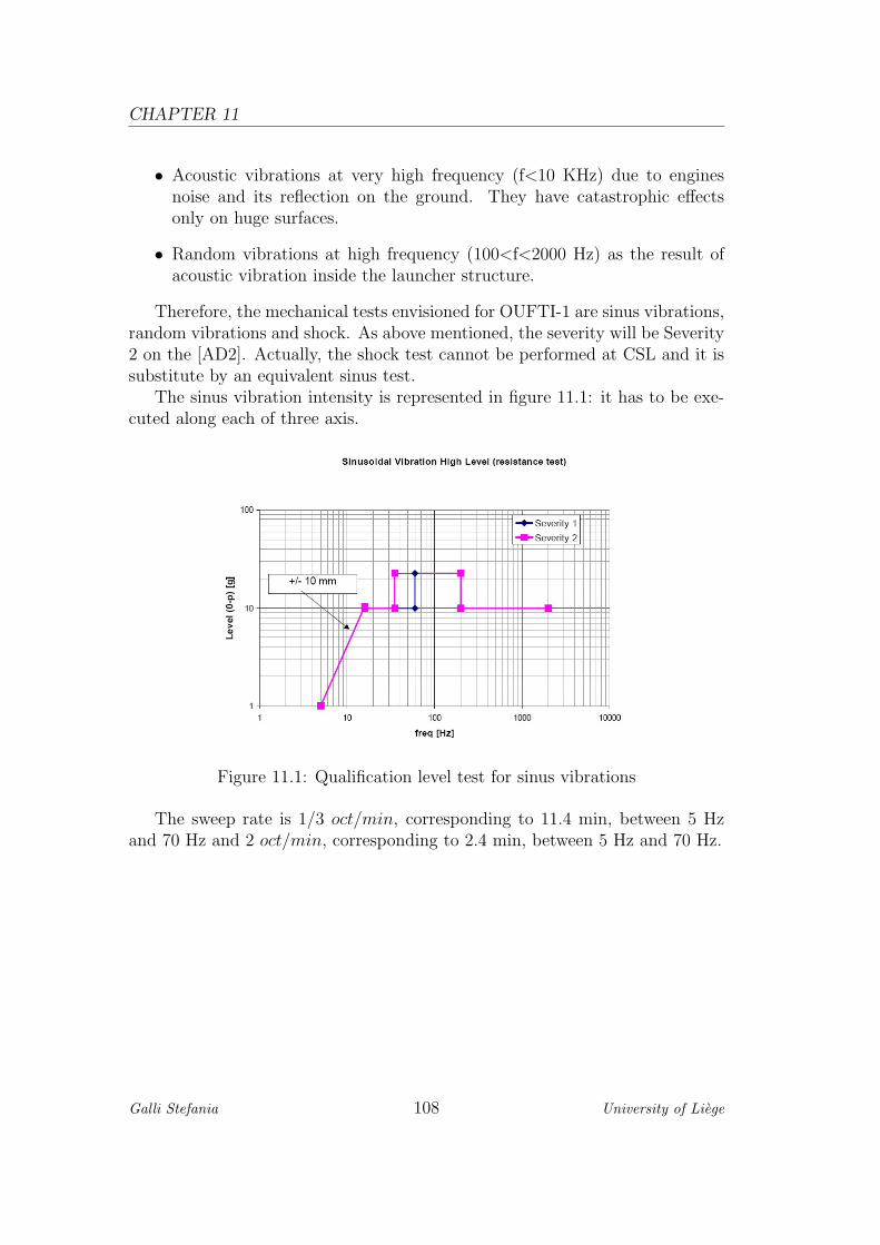
CHAPTER 11
• Acoustic vibrations at very high frequency (f<10 KHz) due to enginesnoise and its reflection on the ground. They have catastrophic effectsonly on huge surfaces.
• Random vibrations at high frequency (100<f<2000 Hz) as the result ofacoustic vibration inside the launcher structure.
Therefore, the mechanical tests envisioned for OUFTI-1 are sinus vibrations,random vibrations and shock. As above mentioned, the severity will be Severity2 on the [AD2]. Actually, the shock test cannot be performed at CSL and it issubstitute by an equivalent sinus test.
The sinus vibration intensity is represented in figure 11.1: it has to be exe-cuted along each of three axis.
Figure 11.1: Qualification level test for sinus vibrations
The sweep rate is 1/3 oct/min, corresponding to 11.4 min, between 5 Hzand 70 Hz and 2 oct/min, corresponding to 2.4 min, between 5 Hz and 70 Hz.
Galli Stefania 108 University of Liege
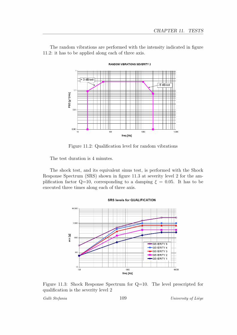
CHAPTER 11. TESTS
The random vibrations are performed with the intensity indicated in figure11.2: it has to be applied along each of three axis.
Figure 11.2: Qualification level for random vibrations
The test duration is 4 minutes.
The shock test, and its equivalent sinus test, is performed with the ShockResponse Spectrum (SRS) shown in figure 11.3 at severity level 2 for the am-plification factor Q=10, corresponding to a damping ξ = 0.05. It has to beexecuted three times along each of three axis.
Figure 11.3: Shock Response Spectrum for Q=10. The level prescripted forqualification is the severity level 2
Galli Stefania 109 University of Liege

CHAPTER 11
11.3 Environmental tests
The space environment is extremely hostile for a satellite: radiations, thermalcycling and vacuum are the main problems. Especially the electronic equipmentare sensible as they have narrow temperature limits and often suffer of damagesdue to radiations.Given that all the material used on OUFTI-1 will be among the approved ma-terial of NASA in order to avoid an excessive out-gassing, the behavior of thespacecraft and of the payload need to be carefully tested. Environmental testinclude thermal vacuum, thermal cycling and other more mission oriented testsas rain and humidity test.For OUFTI-1 thermal-vacuum and thermal cycling are combined with a ther-mal balance test in a single vacuum sequence.
The thermal vacuum test level for acceptance test are indicated in table11.1. The duration of the acceptance test to use for the PFM test is 2 hours.
Table 11.1: Thermal vacuum qualification test for the PFM.
Number of cycles 4Maximum Temperature Tmax 70CMinimum Temperature Tmin 20C
Duration at Tmax 2hDuration at Tmin 2h
Temperature rate (heating) < 20C/min (internal),> 20C/min (external)Temperature rate (cooling) 2÷ 3C/min
The thermal cycling level for acceptance are indicated in table 11.2. Theduration of the acceptance test to use for the PFM test is 2 hours.
Table 11.2: Thermal cycling qualification test
Number of cycles 10Maximum Temperature Tmax 70CMinimum Temperature Tmin 20C
Duration at Tmax 2hDuration at Tmin 2h
Temperature rate (heating) < 20C/min (internal),> 20C/min (external)Temperature rate (cooling) 2÷ 3C/min
Stabilization criterion 1C/1h
Galli Stefania 110 University of Liege

CHAPTER
12
FUTURE DEVELOPMENTS
The feasibility study of a satellite is only the first step of the design of a spacemission: starting from it, a detailed study needs to be performed.If the structure’s CAD model is already available as we are using an off-the-shelfstructure, the location and the number of the electronic boards and of the pay-load has not been decided yet. Once it will be known, a detailed modal studycan be carried out in order to identify the eigenmodes and the eigenfrquenciesand to verify with a finite elements analysis the resistance to the flight loads.The antennas deployment system design represents another challenging task:they will be in fact wrapped around contact points and maintained in thisconfiguration using the deployment mechanism. Their foreseen position in themiddle of the faces between the two solar cells needs still to be verified: this isin fact the best solution on the communication point of view but not necessaryon the mechanical and energetic ones. Furthermore, if their position won’t bealigned with the gravity center, additional attitude problems can appear duringdeployment: in fact, unless opposite antennas are deployed simultaneously, atorque would be generated.A decision about the attitude control has also to be taken as soon as possiblein order to begin the design of the control system or to foreseen a satellite tum-bling in space.The thermal design based on the complete model has also to be detailed inorder to choose between black and golden painting or to plan a combination ofthe two.The electric and electronic hardware as well as the solar cell type must be fixed:only with a precise estimation of efficiencies and losses, we will know the exactpower available.
111
CHAPTER 12
All these tasks will be accomplish with a tight cooperation between universityand industries: in particular, Thales-Alenia Space ETCA in Charleroi for theelectrical power subsystem, the Liege Space Center for the thermal control andthe choice of future payloads, Spacebel in Liege for the on board data handling,LuxSpace for the mission analysis, Open-Engineering in Liege for the attitudecontrol and V2i in Liege for the structure and configuration subsystem.Anyway, all these future developments need more information on the payload,not available at the moment. A satellite is in fact its payload and, withoutit, it hasn’t any reason to exist. All the design has to be conducted on thebase of payload’s requirements and in order to give him the best conditions toaccomplish its mission. The first and more important step is therefore to havea precise configuration of the D-STAR system and to know its limits. Only inthis way, we will be able to evaluate if the power produced is enough, if thedoppler effect without attitude control is too high and how much we need toshield the payload from radiations.
12.1 Possible payloads
The foreseen payloads of the future missions of LEODIUM Project deserve aseparate treatment. In fact, mass and power available on a CubeSat make thisevaluation quite complicate.Among the university departments, the interest is mainly concentrated on Micro-Electro-Mechanical Systems (MEMS) and on granular material. The former isparticularly suitable for a nanosatellite: so small actuators and sensors can infact be used to control the satellite and we can in this way test their behaviorin space and their resistance to external environment before employing them onmore ambitious missions.The ideal target for a CubeSat mission is in fact a technology demonstrationor testing a recently developed element. The project is cheap and its goal ismainly educational to give students hand-on experience: placing on a CubeSatnon space-tested elements that risk to cause the satellite failure is much lessdramatic than chance loosing a bigger mission. In fact, even if the mission fails,students have taken advantage of the acquired experience.Among the possible technology demonstration payloads, the most interestingseems to be some MEMS for attitude control system’s sensors and actuators,active antennas and thermal sensors and magnetometers.Also testing into space some active damping systems seems interesting: one ofthe main problems in space is in fact that the viscous damping of a structuredisappears and only the structural damping remains. As a result, structuresthat on the earth are sufficiently damped, in space need some added dampersto avoid excessive vibrations as well as damping systems are less effective into
Galli Stefania 112 University of Liege
CHAPTER 12. FUTURE DEVELOPMENTS
space. This kind of test has already been done into space: in particular Profes-sor Preumont of Bruxelles University placed an active vibration damper on theSpace Shuttle to test it. Testing a miniaturized version of the same system ona CubeSat would have probably been much less expensive.The test of advanced solar cells is also a kind of mission target that perfectlyfits a CubeSat: their effective efficiency in orbit can be determined as well astheir hardness to radiations.Some nanosatellite missions are also used for testing micropropulsors but theycannot be launched using a Pico Orbital Deployer and finding a launch becomesmore complicate.Last but not least, a CubeSat can be equipped just like all the other satelliteswith a scientific payload on board. In this case, the most difficult task is to finda suitable instrument. Placing a camera and taking pictures of the earth is cer-tainly a good idea on the educational point of view as the mission design wouldbe exactly like the one of a bigger satellite with all the requirement of pointingprecision and stability, but the scientific result wouldn’t be innovative: manyother satellites do the same thing but they employ cameras with much higherresolution. Depending on the orbit, the study of earth radiation environmentor of the gravitational and magnetic fields can also be interesting. Formationflight is another possibility but it demands much more resources as multiplesatellites are launched at the same time.Finally, a CubeSat is suitable for many different payloads but they need tohave compatible dimensions and weight: a dedicated design phase is thereforenecessary.
Galli Stefania 113 University of Liege


CHAPTER
13
CONCLUSIONS
This work constitutes a complete feasibility study for the CubeSat OUFTI-1.The goal was to demonstrate that with the assigned orbit, we can effectivelydesign, build and operate the satellite.We analyzed the orbit and its evolution in time: we obtained a lifetime of 4.2years, a field of view length of up to more than 6000 Km and an available com-munication time with the ground station in Liege of up to 104 min/day. A studyon the radiation environment has also been carried out to identify the neces-sary thickness of shielding material. The structure and the deployment systemhave been discussed, as well as the attitude control feasibility. Furthermore, wecalculated the power available: OUFTI-1 disposes continuously of 1.3 W. Themaximal and minimal satellite’s temperature in orbit have been estimated fordifferent coatings with a nodes model: among the acceptable solutions we havea temperature range between 255K in the cold case with black coating and 307K in the hot case with golden coating. Thanks to the link budget, we know thatthe available power is enough to guarantee a good communication between theomnidirectional antennas of the satellite on the assigned orbit and the groundstation. Finally the different tests have been presented.The results show that the design is feasible and that the mission could effec-tively work with the available power and mass. Some effort need to be done tooptimize the payload efficiency but the mission target can be reached.
On the educational point of view, the goal has definitely been achieved: weexperienced in fact the participation to a real satellite design phase and to ateam work. Furthermore some external events as the CubeSat workshop atthe European Space Technology Research Center were really challenging butmotivating tasks.
115

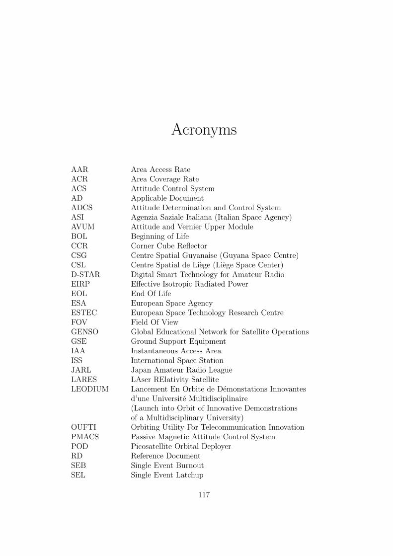
Acronyms
AAR Area Access RateACR Area Coverage RateACS Attitude Control SystemAD Applicable DocumentADCS Attitude Determination and Control SystemASI Agenzia Saziale Italiana (Italian Space Agency)AVUM Attitude and Vernier Upper ModuleBOL Beginning of LifeCCR Corner Cube ReflectorCSG Centre Spatial Guyanaise (Guyana Space Centre)CSL Centre Spatial de Liege (Liege Space Center)D-STAR Digital Smart Technology for Amateur RadioEIRP Effective Isotropic Radiated PowerEOL End Of LifeESA European Space AgencyESTEC European Space Technology Research CentreFOV Field Of ViewGENSO Global Educational Network for Satellite OperationsGSE Ground Support EquipmentIAA Instantaneous Access AreaISS International Space StationJARL Japan Amateur Radio LeagueLARES LAser RElativity SatelliteLEODIUM Lancement En Orbite de Demonstations Innovantes
d’une Universite Multidisciplinaire(Launch into Orbit of Innovative Demonstrationsof a Multidisciplinary University)
OUFTI Orbiting Utility For Telecommunication InnovationPMACS Passive Magnetic Attitude Control SystemPOD Picosatellite Orbital DeployerRD Reference DocumentSEB Single Event BurnoutSEL Single Event Latchup
117

CHAPTER 13
SEP Single Event PhenomenaSEU Single Event UpsetSPENVIS SPace ENVironment Information SystemSRS Shock Response SpectrumSSO Sun Synchronous OrbitVEGA Vettore Europeo di Generazione Avanzata
(European Vehicle of Advanced Generation)
Galli Stefania 118 University of Liege

BIBLIOGRAPHY
[1] Wiley J. Larson, James R. Wertz, Space Mission Analysis and Design,third ed., Springer, Space Technology Library, 1999
[2] James R. Wertz, Spacecraft Attitude Determination and Control, Springer,Space Technology Library, 1978
[3] Vladimir A. Chobotov, Orbital Mechanics, American Institute of Aeronau-tics and Astronautics, 2002
[4] James R. Wertz, Mission Geometry Orbit and Constellation Design Man-agement, Springer, Space Technology Library, 2001
[5] P. Rochus, V. Rochus, Controle thermique spatial, notes of Conceptiond’experiences spatiales classes, University of Liege
[6] P. Rochus, Effet de l’environnement spatial sur la conception, notes ofConception d’experiences spatiales classes, University of Liege
APPLICABLE DOCUMENTS
[AD1] Vega User’s Manual, Issue 3, Rev. 0, March 2006
[AD2] Vega Launch Vehicle Program General Specification: Qualification andAcceptance Test of Equipments (VG-SG-1-C-040-SYS), Issue 5, Rev. 1, 13November 2006
[AD3] Poly Picosatellite Orbital Deployer Interface Control Document, Issue 1,11 February 2004
[AD4] CubeSat Design Specification, Rev. 10, 2 August 2006
[AD5] Cubesat P-POD Deployer Requirements, May 2002
REFERENCE DOCUMENTS
119

CHAPTER 13
[RD1] Stefania Galli, Jonathan Pisane, D-STAR based student CubeSat of theUniversity of Liege, CubeSat Workshop, ESTEC, Noordwijk, NL, 22-24January 2008
[RD2] Educational Payload on the Vega Maiden Flight. Call for CubeSat Pro-posal
[RD3] Stefania Galli, Philippe Ledent, Jonathan Pisane, The D-STAR basedstudent CubeSat of the University of Liege (Leodium Project), 17 Mars2008
[RD4] S.Galli, J. Pisane, P. Ledent, A. Denis, J.F. Vandenrijt, P. Rochus, J.Verly, G. Kerschen, L. Halbach, OUFTI-1: The CubeSat developed at theUniversity of Liege, 5th Annual CubeSat Developers’ Workshop, San LuisObispo, USA, 9-11 April 2008
[RD5] Jonathan Pisane, Design and implementation of the terrestrial and spacetelecommunication components of the student nanosatellite of the Univer-sity of Liege
Galli Stefania 120 University of Liege
Acknowledgments
I would like to thank all the members of the OUFTI-1 team for their sup-port and cooperation, in particular the original group: Amandine Denis, Mr.Luc Halbach, Prof. Gaetan Kerschen, Philippe Ledent, Jonathan Pisane, Prof.Pierre Rochus, Jean-Francois Vandenrijt and Prof. Jacques Verly. Withoutthem this project wouldn’t have been possible.
I would like in particular to express my gratitude to my supervisor, Prof.Pierre Rochus, whose expertise, understanding, and patience, added consider-ably to my graduate experience.
I also acknowledge all the employees of the Liege Space Center, where thiswork took from, for their helpfulness and kindness in answering to all my ques-tions.
A final special thanks goes to my family as without their support and en-couragement I wouln’t probably be in Liege.
121