Embed Size (px)
Citation preview
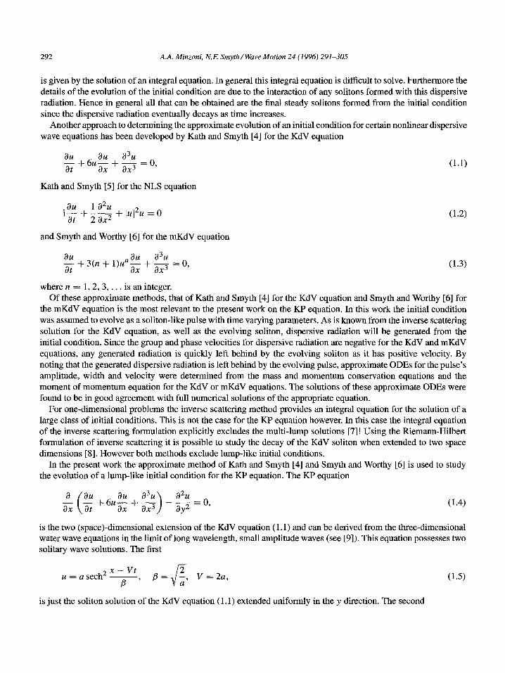
Wave Motion 24 (1996) 291-305
Evolution of lump solutions for the KP equation
A.A. Minzoni a,*, N.F. Smyth b a Department of Mathematics and Mechanics, IIMAS, National Autonomous University of Mexico, Apdo. 20-726, Del. Alvaro Obregon,
01000 Mexico D.E, Mexico b Department of Mathematics and Statistics, The King’s Buildings, University of Edinburgh, Edinburgh EH9 3J2, UK
Received 17 July 1995; revised 29 April 1996
Abstract
The two (space)-dimensional generalisation of the Korteweg-de Vries (KdV) equation is the Kadomtsev-Petviashvili (KP) equation. This equation possesses two solitary wave type solutions. One is independent of the direction orthogonal to the direction of propagation and is the soliton solution of the KdV equation extended to two space dimensions. The other is a true two-dimensional solitary wave solution which decays to zero in all space directions. It is this second solitary wave solution which is considered in the present work. It is known that the KP equation admits an inverse scattering solution. However this solution only applies for initial conditions which decay at infinity faster than the reciprocal distance from the origin. To study the evolution of a lump-like initial condition, a group velocity argument is used to determine the direction of propagation of the linear dispersive radiation generated as the lump evolves. Using this information combined with conservation equations and a suitable trial function, approximate ODES governing the evolution of the isolated pulse are derived. These pulse solutions have a similar form to the pulse solitary wave solution of the KP equation, but with varying parameters. It is found that the pulse solitary wave solutions of the KP equation are asymptotically stable, and that depending on the initial conditions, the pulse either decays to a pulse of lower amplitude (shedding mass) or narrows down (shedding mass) to a pulse of higher amplitude. The solutions of the approximate ODES for the pulse evolution are compared with full numerical solutions of the IQ equation and good agreement is found.
1. Introduction
A number of equations describing nonlinear wave propagation, among them the Korteweg-de Vries (KdV) equa- tion, the nonlinear Schrijdinger (NLS) equation, the Sine-Gordon equation and the Kadomtsev-Petviashvili (KP) equation, possess exact solutions via the inverse scattering transform (see [l-3]). While these inverse scattering solutions give information about the solutions of the governing equations, for example the soliton property whereby N solitary wave solutions will interact without change of form, in general it is difficult to obtain the details of the evolution of an initial condition when dispersive radiation is generated. This is because for an arbitrary initial condition, any solitons formed are given by the solution of an eigenvalue problem consisting of an ordinary differ- ential equation (s) plus zero boundary conditions at plus and minus infinity, but any dispersive radiation generated
* Corresponding author.
01652125/96/$15.00 0 1996 Elsevier Science B.V. All rights reserved PZZSO165-2125(96)00023-6
292 A.A. Minzoni, N.E Smyth/Wave Motion 24 (1996) 291-305
is given by the solution of an integral equation. In general this integral equation is difficult to solve. Furthermore the details of the evolution of the initial condition are due to the interaction of any solitons formed with this dispersive radiation. Hence in general all that can be obtained are the final steady solitons formed from the initial condition since the dispersive radiation eventually decays as time increases.
Another approach to determining the approximate evolution of an initial condition for certain nonlinear dispersive wave equations has been developed by Kath and Smyth [4] for the KdV equation
Kath and Smyth [5] for the NLS equation
and Smyth and Worthy [6] for the mKdV equation
$ + 3(n + l)u”Z + 2 = 0,
(1.1)
(1.2)
(1.3)
where n = 1,2,3, . . . is an integer.
Of these approximate methods, that of Kath and Smytb [4] for the KdV equation and Smyth and Worthy [6] for the mKdV equation is the most relevant to the present work on the KP equation. In this work the initial condition was assumed to evolve as a soliton-like pulse with time varying parameters. As is known from the inverse scattering solution for the KdV equation, as well as the evolving soliton, dispersive radiation will be generated from the initial condition. Since the group and phase velocities for dispersive radiation are negative for the KdV and mKdV equations, any generated radiation is quickly left behind by the evolving soliton as it has positive velocity. By noting that the generated dispersive radiation is left behind by the evolving pulse, approximate ODES for the pulse’s amplitude, width and velocity were determined from the mass and momentum conservation equations and the moment of momentum equation for the KdV or mKdV equations. The solutions of these approximate ODES were found to be in good agreement with full numerical solutions of the appropriate equation.
For one-dimensional problems the inverse scattering method provides an integral equation for the solution of a large class of initial conditions. This is not the case for the KP equation however. In this case the integral equation of the inverse scattering formulation explicitly excludes the multi-lump solutions [7]! Using the Riemann-Hilbert formulation of inverse scattering it is possible to study the decay of the KdV soliton when extended to two space dimensions [S]. However both methods exclude lump-like initial conditions.
In the present work the approximate method of Kath and Smyth [4] and Smyth and Worthy [6] is used to study the evolution of a lump-like initial condition for the KP equation. The KP equation
& g+6.:+% -$=O, ( >
(1.4)
is the two (space)-dimensional extension of the KdV equation (1.1) and can be derived from the three-dimensional water wave equations in the limit of long wavelength, small amplitude waves (see [9]). This equation possesses two solitary wave solutions. The first
x - Vt u=asech2------,
B (1.5)
is just the soliton solution of the KdV equation (1.1) extended uniformly in the y direction. The second
A.A. Minzoni, N.E Smyth/Wave Motion 24 (1996) 291-305 293
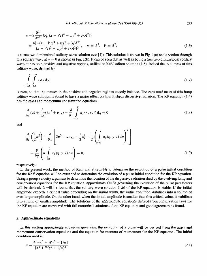
* = 2~~1%1(~ - Vt)2 + wy2 + 3/A2])
4[-(x - Vt)2 + wy2 + 3/A2]
= [(x - vt)2 + wy2 + 3/A2]2 7 w = A2, V = A2, (1.6)
is a true two-dimensional solitary wave solution (see [ 11). This solution is shown in Fig. 1 (a) and a section through this solitary wave at y = 0 is shown in Fig. l(b). It can be seen that as well as being a true two-dimensional solitary wave, it has both positive and negative regions, unlike the KdV soliton solution ( 1.5). Indeed the total mass of this solitary wave, defined by
coo0
ss ud.xdy, (1.7)
--oo --co
is zero, so that the masses in the positive and negative regions exactly balance. The zero total mass of this lump solitary wave solution is found to have a major effect on how it sheds dispersive radiation. The KP equation (1.4) has the mass and momentum conservation equations
x
+L Y, f> drl = 0 (1.8)
and
(1.9)
respectively. In the present work, the method of Kath and Smyth [4] to determine the evolution of a pulse initial condition
for the KdV equation will be extended to determine the evolution of a pulse initial condition for the KP equation. Using a group velocity argument to determine the location of the dispersive radiation shed by the evolving lump and conservation equations for the KP equation, approximate ODES governing the evolution of the pulse parameters will be derived. It will be found that the solitary wave solution (1.6) of the KP equation is stable. If the initial amplitude exceeds a critical value depending on the initial width, the initial condition stabilises into a soliton of even larger amplitude. On the other hand, when the initial amplitude is smaller than this critical value, it stabilises into a lump of smaller amplitude. The solutions of the approximate equations derived from conservation laws for the KP equation are compared with full numerical solutions of the KP equation and good agreement is found.
2. Approximate equations
In this section approximate equations governing the evolution of a pulse will be derived from the mass and momentum conservation equations and the equation for moment of momentum for the KP equation. The initial condition used is
4[-x2 + WY2 + l/a] Cl=
[X2 + WY2 -t l/a]2 ’ (2.1)
294 A.A. Minzoni, N.E Smyth/Wave Motion 24 (1996) 291-305
O-
(b) -0.2 -60 -40 -20 0 20 40 60
x
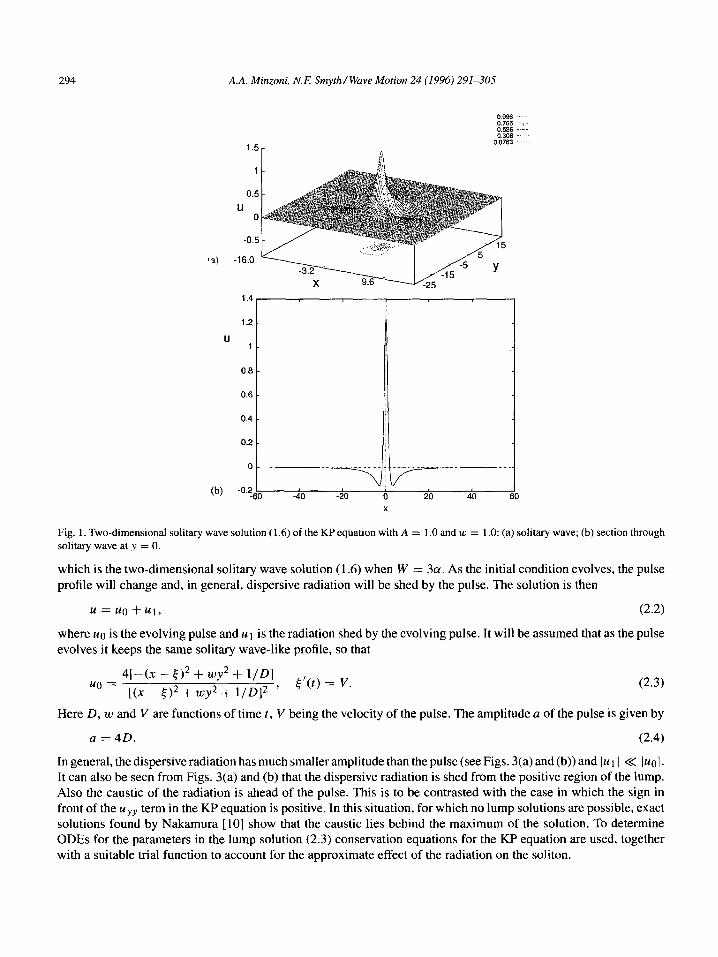
Fig. 1. Two-dimensional solitary wave solution (1.6) of the KP equation with A = I .O and IC = 1 .O: (a) solitary wave; (b) section through
solitary wave at J = 0.
which is the two-dimensional solitary wave solution (1.6) when W = ICY. As the initial condition evolves, the pulse profile will change and, in general, dispersive radiation will be shed by the pulse. The solution is then
u=uo+u1, (2.2)
where ug is the evolving pulse and u 1 is the radiation shed by the evolving pulse. It will be assumed that as the pulse evolves it keeps the same solitary wave-like profile, so that
41-(X - <)* + UJy* + l/o]
ug = 1(x -#+uJy*+1/0]2 ’ C’(l) = v. (2.3)
Here D, w and V are functions of time t, V being the velocity of the pulse. The amplitude a of the pulse is given by
a=4D. (2.4)
In general, the dispersive radiation has much smaller amplitude than the pulse (see Figs. 3(a) and (b)) and 1~ 11 < IuoI. It can also be seen from Figs. 3(a) and (b) that the dispersive radiation is shed from the positive region of the lump. Also the caustic of the radiation is ahead of the pulse. This is to be contrasted with the case in which the sign in front of the uyy term in the KP equation is positive. In this situation, for which no lump solutions are possible, exact solutions found by Nakamura [IO] show that the caustic lies behind the maximum of the solution. To determine ODES for the parameters in the lump solution (2.3) conservation equations for the KP equation are used, together with a suitable trial function to account for the approximate effect of the radiation on the soliton.
A.A. Minzoni, NJ? Smyth/ Wave Motion 24 (1996) 291-305 295
The evolution of pulses for the KP equation presents a number of significant differences from the one-dimensional
evolution for the KdV equation. In the one-dimensional case the radiation extends from the trailing edge of the evolving pulse to x = --co. Also the pulse is always positive and the radiation shed takes mass away from it. The two (space)-dimensional case of the KP equation is different in two fundamental ways. Firstly, since we are now dealing with two space dimensions, the region in which the linear dispersive radiation is confined changes with time. This region will be determined by using a standard group velocity argument. Secondly, the total mass of the lump (2.3) is zero. This immediately raises the question of how can the pulse shed radiation as it evolves. To resolve this question, we observe from Figs. 3(a) and (b) that the radiation is shed from the region in which the pulse is positive and that the negative portion of the lump for x < 0 merges with the radiation. This motivates the assumption (to be verified by comparison with the full solution) that the radiation is shed from the positive part of the pulse located in x 5 l(t), where t(t) is the pulse centre.
In [4,6] it was found from a group velocity argument that linear dispersive radiation only occurs behind the pulse for the KdV and mKdV equations. As there is no radiation in the region from the pulse to x = co, integrating the mass conservation equation from the pulse to x = 00 gives an equation for the pulse parameters without needing any detailed knowledge of the radiation. We observe from Figs. 3(a) and (b) that the front half of the pulse merges with the caustic ahead of it. Thus in the region ahead of the caustic the radiation is negligible (as in clearly shown in the figure). We can therefore integrate the equation for mass conservation (1.8) in this region ahead of the caustic, using the slowly varying soliton (2.3) as a trial function. This will give the first equation for the pulse parameters. To determine this region of integration, we now determine the linear radiation produced by the pulse on approximating it as a source moving with velocity V = i.
Linear radiation for the KP equation satisfies the linearised KP equation
(2.5)
where
g(-x - t(t), Y, t) = -(uot + 6uouox + ~oxxn)x + uoyy. (2.6)
The function g is taken to be slowly varying in t since it is assumed that the pulse parameters and the velocity V = $ are slowly varying functions of time. Since we are interested in the evolution of the caustic alone, the detailed form of g is not needed. Due to the slow time evolution of g, it can be found that ~1 takes the form
co’x
1 Ul(X, Y? t) = (2n)2
ss G(k, I, t)ei[k(x-~(r))+[Y-o(k,l)fl dk dl.
--co -co
(2.7)
The dispersion relation o(k, Z) is given by
l2 w(k, Z) = -k3 - k (2.8)
and the function G, whose specific form is not needed for the present work, is related to g. The caustic for the dispersive radiation is determined by finding the coalescing saddle points for the phase of the
integral (2.7) giving u 1. It is thus found that the caustic is given by
(2.9)
which has the form of a moving, expanding parabola ahead of the pulse. The dispersive radiation then lies behind this caustic, since from (2.8) the x component of the group velocity is negative.
296 A.A. Minzoni, NE Smyth/Wave Motion 24 (1996) 291-30s
We thus consider conservation of mass for the soliton uu in the region ahead of the caustic. The time varying region R(t) ahead of the caustic is --00 5 y 5 00, x 2 i(r) + y2/4t = F(y, t). We therefore obtain
co co d
z ucdxdy = 2; u. dx dy
R(t) b F&Z)
on using symmetry. We thus have on differentiating and substituting for ut from the KP equation (1.4)
d
dt ss u. dx dy
0 F(y.0 00 co 00
zz- s Ftuo(F(y, t), Y> dy - ss (3~; + uoxx)x dx dy
0 0 F(Y.0
On using the definition of F(y, t), this becomes
a
-z. I I uo dx dy
uo(F(y, t>, Y) dy + (3~; + ~O~x)~x=F(y,t) dy
+J 7 { .iuo(n+yldq} dxd:
(2.10)
(2.11)
(2.12)
0 F(y,t) I-co J YY
which is the first equation for the parameters D, w and V. To obtain the equation for the pulse velocity V, we proceed as in [4] by considering the equation for the moment
of momentum MM
d
dt ss xu* dx dy
IZ
SS [4u3 -3(u,)‘]dxdy+ 7 72~~ j uyy(rj,y)drldxdy. (2.13)
--M--co -Lw --co --co
The integrals involved in this expression are evaluated using the change of variable x - c(t) = x’ and then using polar coordinates. In this manner it is found that the velocity of the evolving pulse is given by
V=2Df~w. (2.14)
This expression clearly reduces to the lump solitary wave velocity in the appropriate limit w = 30 (see (1.6)). Moment of momentum rather than moment of mass has been used to determine the velocity of the pulse as it has
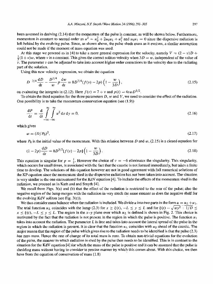
A.A. Minzoni, N.E Smyth/Wave Motion 24 (1996) 291-305 297
been assumed in deriving (2.14) that the momentum of the pulse is constant, as will be shown below. Furthermore, momentum is constant to second order as u2 = ui + 2uuur + UT and uuul = 0 since the dispersive radiation is left behind by the evolving pulse. Since, as shown above, the pulse sheds mass as it evolves, a similar assumption could not be made if the moment of mass equation was used.
At this stage we proceed as in [4] to take a more general expression for the velocity, namely V = (2 - v)D + 4 (1 + u)w, where u is a constant. This gives the correct soliton velocity when 30 = w, independent of the value of u. The parameter 1) can be adjusted to take into account higher order corrections to the velocity due to the radiating part of the solution.
Using this new velocity expression, we obtain the equation
D-314 y D1i4 dw
-_ wpdt = 8D7j4 (f(v) - 2P) (1 - g> , (2.15)
on evaluating the integrals in (2.12). Here f(u) = 7 + u and p(t) = 4twD’/‘. To obtain the third equation for the three parameters D, w and V, we need to consider the effect of the radiation.
One possibility is to take the momentum conservation equation (see (1.9))
dP dooo3
dt=dt ss U2dxdy =O, (2.16)
-co -cQ
which gives
w = (D/Po)~, (2.17)
where PO is the initial value of the momentum. With this relation between D and w, (2.15) is a closed equation for
(1 - 2P)Z = 8D5’2[f(u) -2p] (1 - G).
This equation is singular for p = i. However the choice of v = -6 eliminates the singularity. This singularity, which occurs for small times, is associated with the fact that the caustic is not formed immediately, but takes a finite time to develop. The solutions of this equation however are not in good agreement with full numerical solutions of the Kp equation since the momentum shed in the dispersive radiation has not been taken into account. The situation is very similar to the one encountered for the KdV equation [4]. To include the effects of the momentum shed in the radiation, we proceed as in Kath and and Smyth [4].
We recall from Figs. 3(a) and (b) that the effect of the radiation is restricted to the rear of the pulse; also the negative region of the lump merges with the radiation in very much the same manner as does the negative shelf for the evolving KdV soliton (see Fig. 3(c)).
We thus consider mass balance when the radiation is included. We divide u into two parts in the form u = ur +ul .
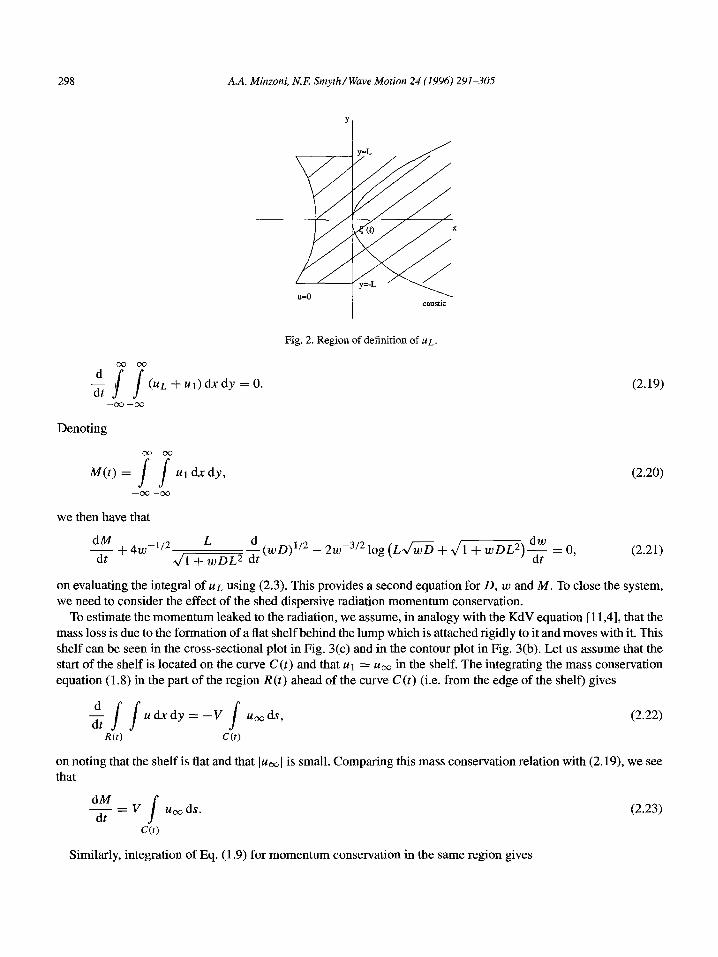
The trial function UL coincides with the lump (2.3) for x 2 c(t), -L 5 y 5 L and for t(t) - dm 5 x 5 t(t), -L 5 y 5 L. The region in the x-y plane over which ur is defined is shown in Fig. 2. This choice is motivated by the fact that the radiation is not present in the region in which the pulse is positive. The function ut takes into account the radiation. The parameter L is free and takes into account the lateral spread of the pulse in the region in which the radiation is present. It is clear that the function UL coincides with uu ahead of the caustic. The major reason that the region of the pulse which gives rise to the radiation needs to be identified is that the pulse (2.3) has zero mass. Hence the rate of change of its total mass is zero. To obtain non-trivial equations for the evolution of the pulse, the manner in which radiation is shed by the pulse then needs to be identified. This is in contrast to the situation for the KdV equation [4] for which the mass of the pulse is positive and it can be assumed that the pulse is shedding mass without having to consider te precise manner by which this comes about. With this choice, we then have from the equation of conservation of mass ( 1.8)
298 A.A. Minzoni, N.E Smyth/Wave Motion 24 (1996) 291-305
x
Fig. 2. Region of definition of EL.
(UL +ul)dxdy =O.
-cxJ -co
Denoting
M(t) = ss ~1 dx dy, --oo -co
we then have that
(2.19)
(2.20)
(2.21)
on evaluating the integral of UL using (2.3). This provides a second equation for D, w and M. To close the system, we need to consider the effect of the shed dispersive radiation momentum conservation.
To estimate the momentum leaked to the radiation, we assume, in analogy with the KdV equation [ 11,4], that the mass loss is due to the formation of a flat shelf behind the lump which is attached rigidly to it and moves with it. This shelf can be seen in the cross-sectional plot in Fig. 3(c) and in the contour plot in Fig. 3(b). Let us assume that the start of the shelf is located on the curve C(t) and that ~1 = uDo in the shelf. The integrating the mass conservation
equation (1.8) in the part of the region R(t) ahead of the curve C(t) (i.e. from the edge of the shelf) gives
(2.22)
on noting that the shelf is flat and that ]uoo 1 is small. Comparing this mass conservation relation with (2.19>, we see that
(2.23)
Similarly, integration of Eq. (1.9) for momentum conservation in the same region gives
A.A. Minzoni, NJ? Smyth/Wave Motion 24 (1996) 291-305
Ei -.: ;:g : : :
0.7 ;:g -: 0.6
0.223 0169 -
u 8::
----
0.3 0.2 0.1
-0.7 -0.2
(a) -51.2
0451 "A",
0 :E 0.5 014 -
u 0.4 o.om ----
0.3 0.2 0.1 0
-0.1
@) -51.2
0.5
Cc) -0.1 !&I -40 -30 -20 -10 0 10 x
0.9
(4
299
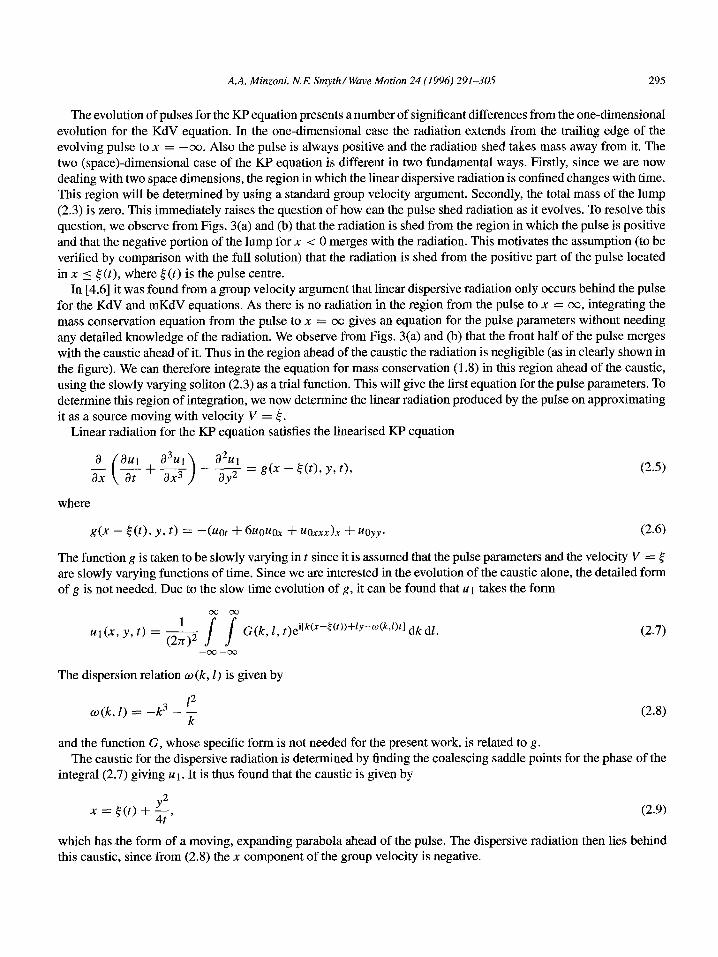
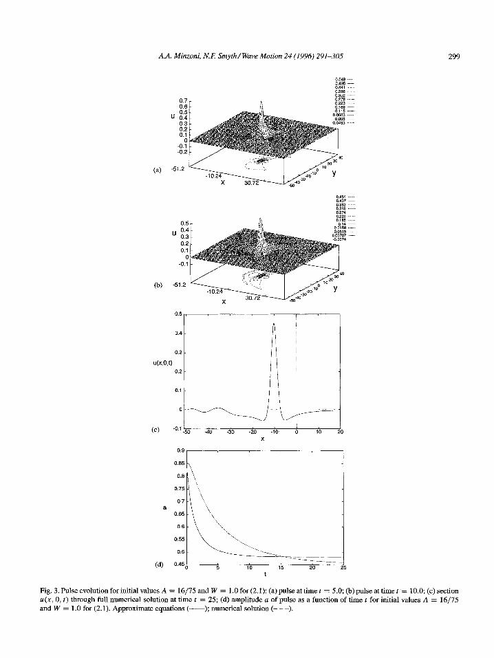
Fig. 3. Pulse evolution for initial values A = 16/75 and W = 1.0 for (2.1): (a) pulse at time t = 5.0; (b) pulse at time t = 10.0; (c) section U(X, 0, t) through full numerical solution at time t = 25; (d) amplitude a of pulse as a function of time f for initial values A = 16/75
and W = 1 .O for (2.1). Approximate equations (-); numerical solution (- - -).
300 A.A. Minzoni, N.E Smyth/Wave Motion 24 (1996) 291-305
d
dt ss 1 2 2~4 dxdy=-V s
‘,” ds 20° ’
(2.24)
R(t) c(t)
on using the same assumptions as just used for mass conservation. To close the system we assume that uoo is approximately constant on a portion I of the curve C(t) located at the rear of the evolving lump (u, cannot be constant all along C(t) since uoo decays to zero as the curve C extends to infinity). We therefore have from (2.23) that
(2.25)
With the added momentum loss (2.24) to radiation, with uoo given by (2.25), the momentum equation (2.16) therefore becomes
-$D@) = --& (z!)’ = _& (.y2. (2.26)
The parameter 4 = Z-l provides an estimate of the importance of the lateral leakage of radiation. The full system of equations for D, w and M is then (2.15), (2.21) and (2.26).
These equations were numerically integrated for a variety of initial conditions. In particular very elongated shapes at t = 0 were used to provide a severe test of the approximation. It was found that the solution of the approximate equations was very insensitive to the value of L, so that these equations have essentially one free parameter, 1. Taking L = 1 was found to be sufficient and gave solutions typical of a wide range of values of L. The solutions of the approximate equations were found to depend weakly on 1 and the approximate value 1 = 0.3 was found to give the best agreement with full numerical solutions of the KP equation, independent of the initial condition used.
In Section 3 some comparisons between solutions of the approximate equations and full numerical solutions of the KF’ equation are shown and discussed. These comparisons show how the crube approximation to the complicated radiation process outlined in this section produces the correct qualitative behaviour and good (comparable with the one-dimensional case [4]) quantitative agreement for the time evolution of the lump amplitude.
3. Numerical method and results
The method used to numerically solve the KP equation (1.4) is an extension of the method used by Kath and Smyth [4] to solve the KdV equation. In this work a pseudo-spectral method was used, based on the method of Fornberg and Whitham [ 121 for the KdV equation. To numerically integrate the KF’ equation (1.4), it is easiest to write it as a system
a~ a224 z=ay2-
(3.1)
(3.2)
The first equation (3.1) is then solved using the melhod of Kath and Smyth [4]. The x-derivatives are evaluated using FFTs and the equation is then propagated forward in time using a 4th order Runge-Kutta scheme. The second equation (3.2) is integrated using a Crank-Nicolson type scheme. This equation is then approximated by
v(x, y, t) = v(x - Ax, y, t) + - u Ax ( f fubh 2(Ayj2
where
(3.3)
A.A. Minzoni, N.F Smyth/Wave Motion 24 (1996) 291-305 301
6
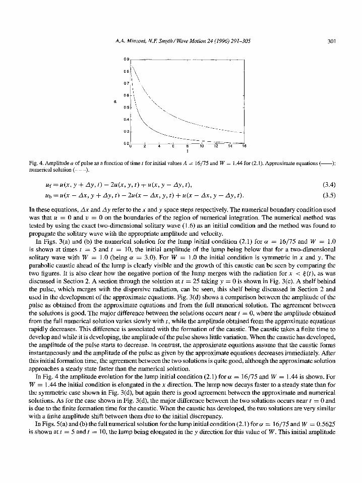
Fig. 4. Amplitude a of pulse as a function of time t for initial values A = 16/75 and W = 1.44 for (2.1). Approximate equations (-); numerical solution (- - -).
uf = u(x, Y + AY, t> - 2u(x, Y, t> + u(x, Y - AY, t>, (3.4)
u,, = u(x - Ax, y -t Ay, t) - 2u(x - Ax, y, t) + u(x - Ax, y - Ay, t). (3.5)
In these equations, An and Ay refer to the x and y space steps respectively. The numerical boundary condition used was that u = 0 and v = 0 on the boundaries of the region of numerical integration. The numerical method was tested by using the exact two-dimensional solitary wave (1.6) as an initial condition and the method was found to propagate the solitary wave with the appropriate amplitude and velocity.
In Figs. 3(a) and (b) the numerical solution for the lump initial condition (2.1) for cz = 16/75 and W = 1.0
is shown at times t = 5 and t = 10, the initial amplitude of the lump being below that for a two-dimensional solitary wave with W = 1.0 (being a! = 3.0). For W = 1.0 the initial condition is symmetric in x and y. The parabolic caustic ahead of the lump is clearly visible and the growth of this caustic can be seen by comparing the two figures. It is also clear how the negative portion of the lump merges with the radiation for x < c(t), as was discussed in Section 2. A section through the solution at t = 25 taking y = 0 is shown in Fig. 3(c). A shelf behind the pulse, which merges with the dispersive radiation, can be seen, this shelf being discussed in Section 2 and used in the development of the approximate equations. Fig. 3(d) shows a comparison between the amplitude of the pulse as obtained from the approximate equations and from the full numerical solution. The agreement between the solutions is good. The major difference between the solutions occurs near t = 0, where the amplitude obtained from the full numerical solution varies slowly with t, while the amplitude obtained from the approximate equations rapidly decreases. This difference is associated with the formation of the caustic. The caustic takes a finite time to develop and while it is developing, the amplitude of the pulse shows little variation. When the caustic has developed, the amplitude of the pulse starts to decrease. In contrast, the approximate equations assume that the caustic forms instantaneously and the amplitude of the pulse as given by the approximate equations decreases immediately. After this initial formation time, the agreement between the two solutions is quite good, although the approximate solution approaches a steady state faster than the numerical solution.
In Fig. 4 the amplitude evolution for the lump initial condition (2.1) for a! = 16/75 and W = 1.44 is shown. For W = 1.44 the initial condition is elongated in the x direction. The lump now decays faster to a steady state than for the symmetric case shown in Fig. 3(d), but again there is good agreement between the approximate and numerical solutions. As for the case shown in Fig. 3(d), the major difference between the two solutions occurs near t = 0 and is due to the finite formation time for the caustic. When the caustic has developed, the two solutions are very similar with a finite amplitude shift between them due to the initial discrepancy.
In Figs. 5(a) and (b) the full numerical solution for the lump initial condition (2.1) for a! = 16/75 and W = 0.5625 is shown at t = 5 and t = 10, the lump being elongated in the y direction for this value of W. This initial amplitude
302 A.A. Minzoni, N.E Smyth/Wave Motion 24 (1996) 291-305
a
Cc) 0.841 I 2 4 6 8 10 12 14
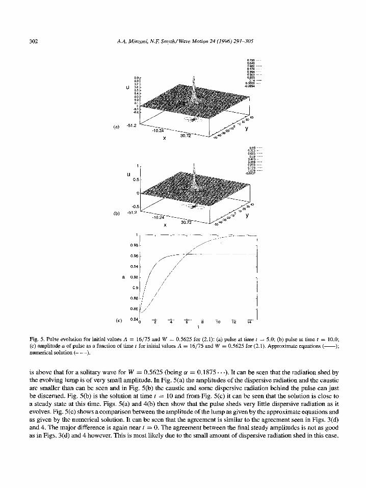
Fig. 5. Pulse evolution for initial values A = 16/75 and W = 0.5625 for (2.1): (a) pulse at time t = 5.0; (b) pulse at time t = 10.0; (c) amplitude a of pulse as a function of time t for initial values A = 16/75 and W = 0.5625 for (2.1). Approximate equations (-); numerical solution (- - -).
is above that for a solitary wave for W = 0.5625 (being a! = 0.1875 . . .). It can be seen that the radiation shed by the evolving lump is of very small amplitude. In Fig. 5(a) the amplitudes of the dispersive radiation and the caustic are smaller than can be seen and in Fig. 5(b) the caustic and some dispersive radiation behind the pulse can just be discerned. Fig. 5(b) is the solution at time t = 10 and from Fig. 5(c) it can be seen that the solution is close to a steady state at this time. Figs. 5(a) and 4(b) then show that the pulse sheds very little dispersive radiation as it evolves. Fig. 5(c) shows a comparison between the amplitude of the lump as given by the approximate equations and as given by the numerical solution. It can be seen that the agreement is similar to the agreement seen in Figs. 3(d) and 4. The major difference is again near t = 0. The agreement between the final steady amplitudes is not as good as in Figs. 3(d) and 4 however. This is most likely due to the small amount of dispersive radiation shed in this case,
A.A. Minzoni, N.E Smyth/Wave Motion 24 (1996) 291-305 303
(a) -51.2
0.14 ...-. 0.108 oom--- 0.0429 0.0104
0.2 O.P21
0.15 0.1
0.05
u 0 -0.05 -0.1
-0.15
(b) -51.2
0.1
0.05
U
0
-0.05 -51.2
Cc) -0.1
0.35
0.3 - I
0.25 - ~WJ) o,2:
0.15 -
0.1 - 1
0.05 -
O-
-0.05 - 1/
0.1 -
-0.15 -
Cd) -o.z-So -40 -20 0 20 40 60
a
W OO i 6 i i $ h i 8 i t
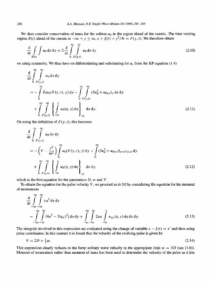
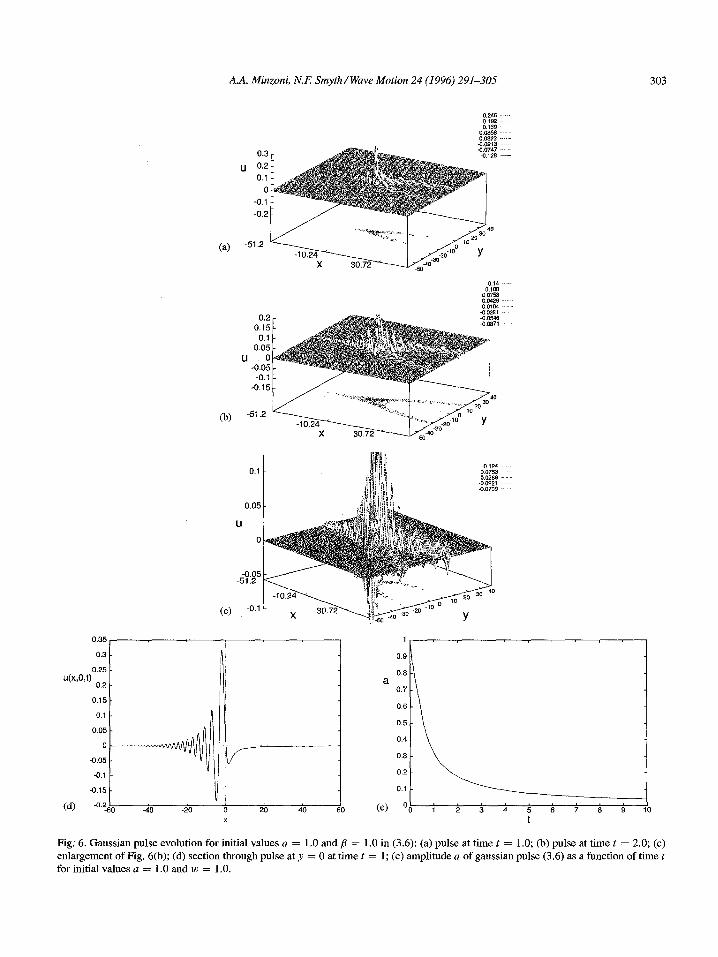
Fig. 6. Gaussian pulse evolution for initial values a = 1.0 and B = 1.0 in (3.6): (a) pulse at time t = 1.0; (b) pulse at time t = 2.0; (c) enlargement of Fig. 6(b); (d) section through pulse at y = 0 at time f = 1; (e) amplitude a of gaussian pulse (3.6) as a function of time t for initial values a = 1.0 and UJ = 1.0.
304 A.A. Minzoni, N.E Smyth/Wave Motion 24 (1996) 291-305
which implies that hte evolution of the pulse is not driven to the same extent by the caustic as in the previous two cases. Nevertheless, the agreement between the two solutions is quite good.
The main prediction of our approximate equations regards the stability of the two-dimensional solitary wave solution of the Kp equation. For cr < W/3 our approximate equations predict that the initial condition (2.1) will decay into a smaller lump soliton, while for a > W/3 they predict that the amplitude of the lump will become larger until it settles to a new lump soliton of higher amplitude.
Fig. 6 shows the evolution of a Gaussian initial condition of the form
u(x, y, 0) = ae-B(x2+y2).
The solution u at t = 1 and t = 2 is shown in Figs. 6(a) and (b), respectively and the time evolution of the gaussian initial condition can be seen. Since radiation is focused at the caustic, there is a large amount of dispersive radiation moving along it. Radiation is then shed at the rear of the evolving pulse to conserve momentum. Fig. 6(c) is an enlargement of Fig. 6(b) in the u direction with the view point rotated around toward the caustic. It can be seen that the train of waves along the caustic is dispersive radiation, not a modulated train of lump solitary waves. Fig. 6(d) shows a cross section of the solution taken through y = 0 at t = 1. The waves behind the pulse can be clearly seen and from this plot it is clear that this radiation is dispersive radiation rather than a train of lump solitons. The gaussian initial condition (3.6) thus appears to be breaking up into dispersive radiation, which is further confirmed by the amplitude behaviour shown in Fig. 6(e). This decay of the gaussian initial condition is consistent with the result from inverse scattering that if the initial condition decays fast enough at infinity, then the solution decays into dispersive radiation alone if the initial amplitude is small enough [7,8]. Fig. 6(e) then shows that even though the initial condition does not have small amplitude in this case, the solution is still decaying into dispersive radiation alone.
In conclusion it has been shown how the ideas of [4,6] can be used to understand and approximate the evolution of lump initial conditions for two-dimensional problems which have not been studied (to date) by other methods. In particular, it has been shown how a very crude approximation to the complicated process of radiation shedding in two dimensions leads to very good quantitative comparisons of the evolution of a two-dimensional pulse with full numerical solutions.
Acknowledgements
N.F. Smyth would like to thank the hospitality of FENOMEC, at Instituto de Investigaciones en Matematicas Aplicadas y en Sistemas of the Universidad National Autonoma de Mexico where this work was carried out.
We are grateful for the comments of a referee which considerably improved the present work.
References
[l] MI. Ablowitz and H. Segur, Solitorzs and the Inverse Scattering Transform, SIAM, Philadelphia, PA (1981).
[2] A.C. Newell, Solitons in Mathematics and Physics, SIAM, Philadelphia, PA (1985).
[3] G.B. Whitham, Linear and Nonlinear Waves, Wiley, New York (1974).
[4] W.L. Katb and N.F. Smyth, “Soliton evolution and radiation loss for the Korteweg-de Vries equation”, Phys. Rev. E 51 (I), 661-670
(1995).
[5] W.L. Katb and N.F. Smyth, “Soliton evolution and radiation loss for the nonlinear Schrodinger equation”, Phys. Rev. E 51 (2), 1484-1492 (1995).
[6] N.F. Smyth and A.L. Worthy, “Solitary wave evolution for mKdV equations”, Wave Motion 21(3), 263-275 (1995).
[7] V.E. Zhakharov and S.V. Manakov, “Soliton Theory” in: Soviet Scientific Reviews, Section A, Vol. I, 133-l 90 (1979).
[8] S. Novikov, S.V. Manokov, L.P. Pitaevskii and V.E. Zhakarov, Theory of Solitons. The Inverse Scattering Method, Plenum, New York (1984). -

A.A. Minzoni, N,E Smyth/Wave Motion 24 (1996) 291-305 305
[9] B.B. Kadomtsev and V.I. Petviashvili, “On the stability of solitary waves in weakly dispersing media”, Soviet Phys. Dokl. 15, 539-541 (1970).
[IO] A. Nakamura, “Decay mode solution of the two dimensional KdV equation and the generalized Bkklund transformation”, J. Math. Phys. 22 (II), 2456-2462 (1981).
[I l] C.J. Knickerbocker and A.C. Newell, “Shelves and the Korteweg-de Vries equation”, J. Fluid Mech. 98,803-818 (1980). [12] B. Fomberg and G.B. Whitham. “A numerical and theoretical study of certain nonlinear wave phenomena”, Philos. Trans. Roy. Sot.
London Sex A 289,373-403 (1978).