Mining Data from Reservoir Simulation Resultsusing R

(to be presented at ICIPEG ’10)

Akmal Aulia, Tham Boon Keat, M. Sanif Maulut,Dr. Noaman El-Khatib, Mazuin Jasamai

EOR Centre, UT PETRONASSupervisor: Prof. Dr. Noaman El-Khatib

June 9th, 2010

Introduction to Association Rules

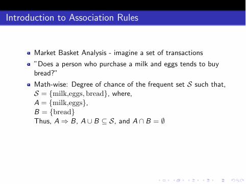
Market Basket Analysis - imagine a set of transactions

”Does a person who purchase a milk and eggs tends to buybread?”

Math-wise: Degree of chance of the frequent set S such that,S = {milk,eggs,bread}, where,A = {milk,eggs},B = {bread}Thus, A ! B, A " B # S, and A $ B = %A ! B is called a ”Rule”

Association Rules in Amazon.com:”Customers who bought this item also bought..”

Introduction to Association Rules

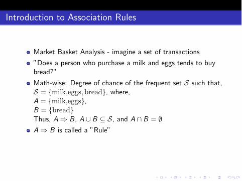
Market Basket Analysis - imagine a set of transactions

”Does a person who purchase a milk and eggs tends to buybread?”

Math-wise: Degree of chance of the frequent set S such that,S = {milk,eggs,bread}, where,A = {milk,eggs},B = {bread}Thus, A ! B, A " B # S, and A $ B = %A ! B is called a ”Rule”

Association Rules in Amazon.com:”Customers who bought this item also bought..”

Introduction to Association Rules

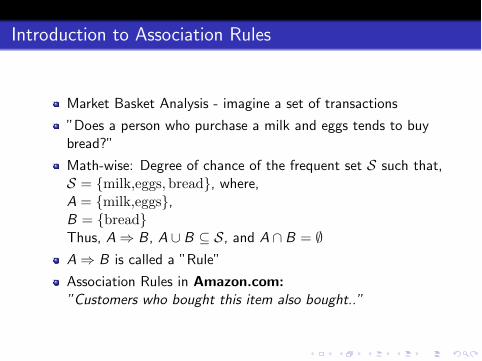
Market Basket Analysis - imagine a set of transactions

”Does a person who purchase a milk and eggs tends to buybread?”

Math-wise: Degree of chance of the frequent set S such that,S = {milk,eggs,bread}, where,A = {milk,eggs},B = {bread}Thus, A ! B, A " B # S, and A $ B = %

A ! B is called a ”Rule”

Association Rules in Amazon.com:”Customers who bought this item also bought..”

Introduction to Association Rules

Market Basket Analysis - imagine a set of transactions

”Does a person who purchase a milk and eggs tends to buybread?”

Math-wise: Degree of chance of the frequent set S such that,S = {milk,eggs,bread}, where,A = {milk,eggs},B = {bread}Thus, A ! B, A " B # S, and A $ B = %A ! B is called a ”Rule”

Association Rules in Amazon.com:”Customers who bought this item also bought..”

Introduction to Association Rules

Market Basket Analysis - imagine a set of transactions

”Does a person who purchase a milk and eggs tends to buybread?”

Math-wise: Degree of chance of the frequent set S such that,S = {milk,eggs,bread}, where,A = {milk,eggs},B = {bread}Thus, A ! B, A " B # S, and A $ B = %A ! B is called a ”Rule”

Association Rules in Amazon.com:”Customers who bought this item also bought..”

Introduction to Association Rules: A Simple Example

Table: Transactional Data Sample

Transaction ID Items1 milk, eggs2 eggs, butter3 peanut4 milk, eggs, bread5 eggs, bread

Support of A = {milk, eggs} = 2 / 5 = 0.4 = 40%

Support of B = {bread} = 3 / 5 = 0.6 = 60%

Support of A ! B = 1/5 = 0.2 =20%

Confidence of A ! B = Support of A!BSupport of A = 0.2

0.4 = 0.5 = 50%

Lift of A ! B = 0.2(0.4)(0.6) = 0.83

Introduction to Association Rules: A Simple Example

Table: Transactional Data Sample

Transaction ID Items1 milk, eggs2 eggs, butter3 peanut4 milk, eggs, bread5 eggs, bread

Support of A = {milk, eggs} = 2 / 5 = 0.4 = 40%

Support of B = {bread} = 3 / 5 = 0.6 = 60%

Support of A ! B = 1/5 = 0.2 =20%

Confidence of A ! B = Support of A!BSupport of A = 0.2

0.4 = 0.5 = 50%

Lift of A ! B = 0.2(0.4)(0.6) = 0.83

Introduction to Association Rules: A Simple Example

Table: Transactional Data Sample

Transaction ID Items1 milk, eggs2 eggs, butter3 peanut4 milk, eggs, bread5 eggs, bread

Support of A = {milk, eggs} = 2 / 5 = 0.4 = 40%

Support of B = {bread} = 3 / 5 = 0.6 = 60%

Support of A ! B = 1/5 = 0.2 =20%

Confidence of A ! B = Support of A!BSupport of A = 0.2

0.4 = 0.5 = 50%

Lift of A ! B = 0.2(0.4)(0.6) = 0.83

Introduction to Association Rules: A Simple Example

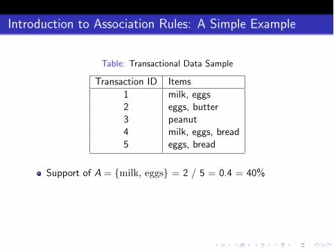
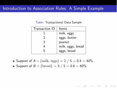
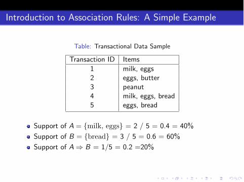
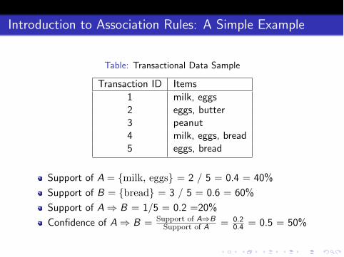
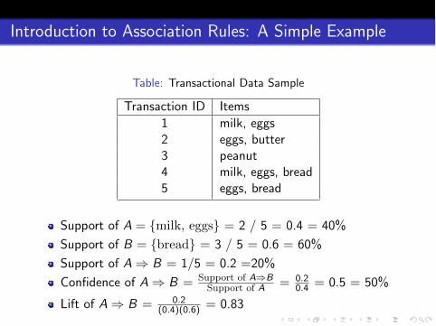
Table: Transactional Data Sample

Transaction ID Items1 milk, eggs2 eggs, butter3 peanut4 milk, eggs, bread5 eggs, bread

Support of A = {milk, eggs} = 2 / 5 = 0.4 = 40%

Support of B = {bread} = 3 / 5 = 0.6 = 60%

Support of A ! B = 1/5 = 0.2 =20%

Confidence of A ! B = Support of A!BSupport of A = 0.2

0.4 = 0.5 = 50%

Lift of A ! B = 0.2(0.4)(0.6) = 0.83

Introduction to Association Rules: A Simple Example

Table: Transactional Data Sample

Transaction ID Items1 milk, eggs2 eggs, butter3 peanut4 milk, eggs, bread5 eggs, bread

Support of A = {milk, eggs} = 2 / 5 = 0.4 = 40%

Support of B = {bread} = 3 / 5 = 0.6 = 60%

Support of A ! B = 1/5 = 0.2 =20%

Confidence of A ! B = Support of A!BSupport of A = 0.2

0.4 = 0.5 = 50%

Lift of A ! B = 0.2(0.4)(0.6) = 0.83

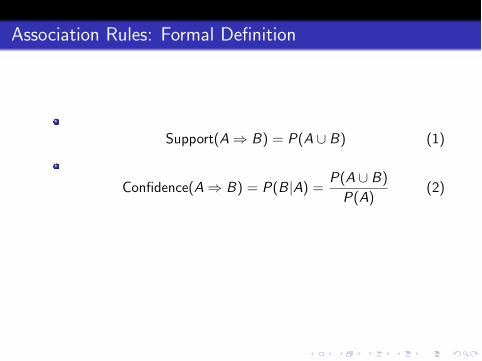
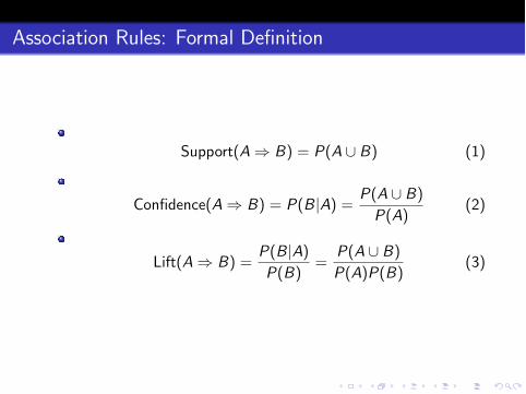
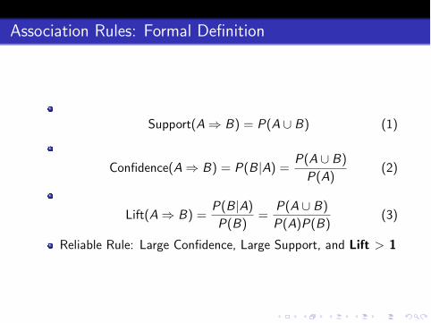
Association Rules: Formal Definition

Support(A ! B) = P(A " B) (1)

Confidence(A ! B) = P(B|A) =P(A " B)

P(A)(2)

Lift(A ! B) =P(B|A)

P(B)=

P(A " B)

P(A)P(B)(3)

Reliable Rule: Large Confidence, Large Support, and Lift > 1

Association Rules: Formal Definition

Support(A ! B) = P(A " B) (1)

Confidence(A ! B) = P(B|A) =P(A " B)

P(A)(2)

Lift(A ! B) =P(B|A)

P(B)=

P(A " B)

P(A)P(B)(3)

Reliable Rule: Large Confidence, Large Support, and Lift > 1

Association Rules: Formal Definition

Support(A ! B) = P(A " B) (1)

Confidence(A ! B) = P(B|A) =P(A " B)

P(A)(2)

Lift(A ! B) =P(B|A)

P(B)=

P(A " B)

P(A)P(B)(3)

Reliable Rule: Large Confidence, Large Support, and Lift > 1

Association Rules: Formal Definition

Support(A ! B) = P(A " B) (1)

Confidence(A ! B) = P(B|A) =P(A " B)

P(A)(2)

Lift(A ! B) =P(B|A)

P(B)=

P(A " B)

P(A)P(B)(3)

Reliable Rule: Large Confidence, Large Support, and Lift > 1

Implementation using R

Language for statistical computing, graphics

GNU General Public License ! FREE!!

Over 2416 contributed packages - ARULES, GA, ANN, etc

Over 106 books published - Bayesian, Monte Carlo, Chemistry

Parallel Computation

Implementation using R

Language for statistical computing, graphics

GNU General Public License ! FREE!!

Over 2416 contributed packages - ARULES, GA, ANN, etc

Over 106 books published - Bayesian, Monte Carlo, Chemistry

Parallel Computation

Implementation using R

Language for statistical computing, graphics

GNU General Public License ! FREE!!

Over 2416 contributed packages - ARULES, GA, ANN, etc

Over 106 books published - Bayesian, Monte Carlo, Chemistry

Parallel Computation

Implementation using R

Language for statistical computing, graphics

GNU General Public License ! FREE!!

Over 2416 contributed packages - ARULES, GA, ANN, etc

Over 106 books published - Bayesian, Monte Carlo, Chemistry

Parallel Computation

Implementation using R

Language for statistical computing, graphics

GNU General Public License ! FREE!!

Over 2416 contributed packages - ARULES, GA, ANN, etc

Over 106 books published - Bayesian, Monte Carlo, Chemistry

Parallel Computation

Mining Data from Reservoir Simulation Results

1 Injection at (1,1), 1 Production at (5,5)

Mining Data from Reservoir Simulation Results

Let reservoir simulation parameter Xi such that i & {1, 2, · · · , 8}.

Table: Description of Parameters

Parameter Description UnitsX1 Surf. rate at inj. well stb/dayX2 Bot. hole pres. limit at the inj. well psiaX3 Liq. rate at the prod. well stb/dayX4 Bot. hole pres. limit at the prod. well psiaX5 Bot. hole pres. datum at the prod. well ftX6 Bot. hole pres. datum at the inj. well ftX7 Inner diameter of the prod. well ftX8 Inner diameter of the inj. well ft

T Final oil recovery (recovery factor)!

OIPt0"OIPt

OIPt0

"

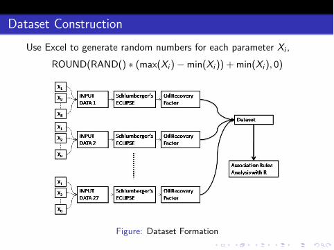
Dataset Construction

Use Excel to generate random numbers for each parameter Xi ,

ROUND(RAND() ' (max(Xi )(min(Xi )) + min(Xi ), 0)

Figure: Dataset Formation

Data Pre-processing

Table: Dataset

X1 X2 X3 X4 X5 X6 X7 X8 T13087 9267 9774 3320 8042 8101 6 5 0.41312082 6192 5943 3844 8058 8030 5 5 0.39713789 5532 4941 2987 8083 8115 4 6 0.37211671 12197 4718 2543 8080 8038 4 6 0.17813182 6055 9507 2989 8057 8040 3 3 0.49211810 7252 7597 4480 8036 8036 6 5 0.42111070 10849 4887 2028 8088 8100 3 5 0.24611861 10220 1545 3723 8117 8045 6 5 0.12412877 6557 8863 3766 8089 8102 4 4 0.46713905 7904 1270 4279 8027 8084 7 3 0.117

... ... ... ... ... ... ... ... ...

Data Pre-processing

Association Rules analyzes Categorical Data. ! Convert it!

Split each parameters by some Xik such thatXi = {Xi1 ,Xi2 , . . . ,Xik , . . . ,Xi8}. Xik can be,

Xik = mean(Xi ) (4)

Xik = median(Xi ) (5)

Thus, )Xi ,

Xik! "=k=

#High(*), for Xik! "=k

> Xik

Low(+), for Xik! "=k, Xik

Data Pre-processing

Association Rules analyzes Categorical Data. ! Convert it!

Split each parameters by some Xik such thatXi = {Xi1 ,Xi2 , . . . ,Xik , . . . ,Xi8}. Xik can be,

Xik = mean(Xi ) (4)

Xik = median(Xi ) (5)

Thus, )Xi ,

Xik! "=k=

#High(*), for Xik! "=k

> Xik

Low(+), for Xik! "=k, Xik

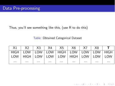
Data Pre-processing

Thus, you’ll see something like this, (use R to do this)

Table: Obtained Categorical Dataset

X1 X2 X3 X4 X5 X6 X7 X8 THIGH LOW LOW LOW HIGH LOW LOW LOW HIGHLOW HIGH LOW LOW LOW HIGH LOW LOW LOW

... ... ... ... ... ... ... ... ...

The ARULES package

Use R’s ARULES package

Apriori algorithm,

i=1Di = {G : G is an itemset of size 1}while Di is not empty do

database pass:for each set in Di , test whether it is frequentlet Fi be the collection of frequent sets from Di

candidate formation:Let Di be those sets of size i + 1 whose all subsets arefrequent

end while

The ARULES package

Use R’s ARULES package

Apriori algorithm,

i=1Di = {G : G is an itemset of size 1}while Di is not empty do

database pass:for each set in Di , test whether it is frequentlet Fi be the collection of frequent sets from Di

candidate formation:Let Di be those sets of size i + 1 whose all subsets arefrequent

end while

Results and Discussion

Table: Limits for the Apriori algorithm’s parameters

Lift Confidence1.5 0.9

! Generated some 24098 rules (for mean-based splitting)

Table: Mean-Based Low-Target (Low Oil Recovery) Yielding

No. Parameter/Value Support Confidence Lift1 X2 *, X5 * 0.148 1.00 1.802 X2 *, X7 + 0.185 1.00 1.803 X1 +, X2 * 0.222 1.00 1.804 X2 *, X4 * 0.222 1.00 1.805 X2 *, X3 + 0.185 1.00 1.806 X5 *, X6 + 0.185 1.00 1.807 X3 +, X7 * 0.222 1.00 1.808 X2 *, X5 *, X8 + 0.037 1.00 1.80

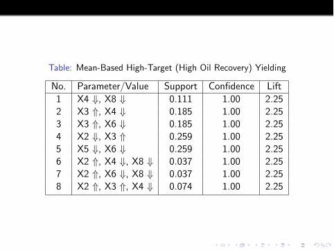
Table: Mean-Based High-Target (High Oil Recovery) Yielding

No. Parameter/Value Support Confidence Lift1 X4 +, X8 + 0.111 1.00 2.252 X3 *, X4 + 0.185 1.00 2.253 X3 *, X6 + 0.185 1.00 2.254 X2 +, X3 * 0.259 1.00 2.255 X5 +, X6 + 0.259 1.00 2.256 X2 *, X4 +, X8 + 0.037 1.00 2.257 X2 *, X6 +, X8 + 0.037 1.00 2.258 X2 *, X3 *, X4 + 0.074 1.00 2.25

Table: Median-Based Low-Target (Low Oil Recovery) Yielding

No. Parameter/Value Support Confidence Lift1 X2 *, X8 * 0.074 1.00 1.932 X5 *, X7 * 0.037 1.00 1.933 X3 +, X7 * 0.111 1.00 1.934 X2 *, X4 * 0.222 1.00 1.935 X2 *, X3 + 0.259 1.00 1.936 X3 +, X6 * 0.259 1.00 1.937 X2 *, X5 *, X8 * 0.037 1.00 1.938 X3 +, X5 *, X8 * 0.074 1.00 1.93

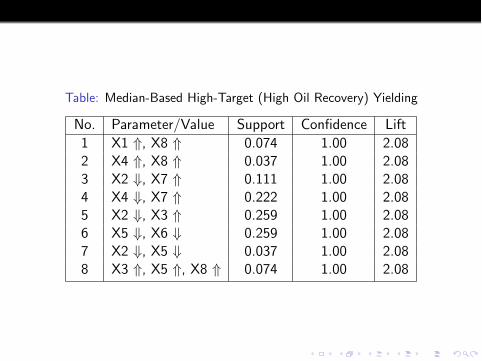
Table: Median-Based High-Target (High Oil Recovery) Yielding

No. Parameter/Value Support Confidence Lift1 X1 *, X8 * 0.074 1.00 2.082 X4 *, X8 * 0.037 1.00 2.083 X2 +, X7 * 0.111 1.00 2.084 X4 +, X7 * 0.222 1.00 2.085 X2 +, X3 * 0.259 1.00 2.086 X5 +, X6 + 0.259 1.00 2.087 X2 +, X5 + 0.037 1.00 2.088 X3 *, X5 *, X8 * 0.074 1.00 2.08

Summary

X2 (BHP limit, INJ) and X3 (liquid rate, PROD) frequentlyshowed up - clue to higher recovery!

More parameters, more wells, a more legitimate study.

Summary

X2 (BHP limit, INJ) and X3 (liquid rate, PROD) frequentlyshowed up - clue to higher recovery!

More parameters, more wells, a more legitimate study.