Minimum Capital Requirements for Market Risk Capital Requirements for Market Risk (BCBS 352, CRR 2 proposal) Frankfurt am Main, May 2017 The “Fundamental review of the trading book”

Minimum Capital Requirements for Market Risk (BCBS 352, CRR 2 proposal)

Frankfurt am Main, May 2017

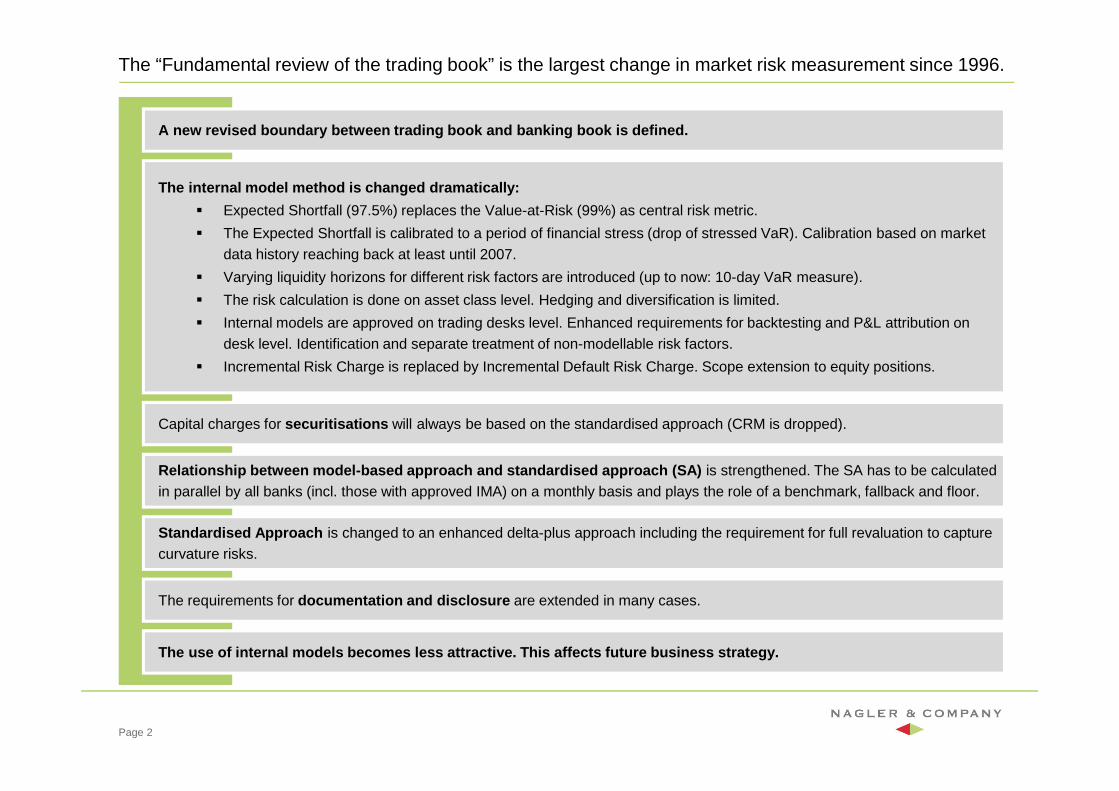
The “Fundamental review of the trading book” is the largest change in market risk measurement since 1996.

Page 2

The use of internal models becomes less attractive. This affects future business strategy.

Capital charges for securitisations will always be based on the standardised approach (CRM is dropped).

Relationship between model-based approach and stand ardised approach (SA) is strengthened. The SA has to be calculated in parallel by all banks (incl. those with approved IMA) on a monthly basis and plays the role of a benchmark, fallback and floor.

The requirements for documentation and disclosure are extended in many cases.

A new revised boundary between trading book and ban king book is defined.

The internal model method is changed dramatically:

� Expected Shortfall (97.5%) replaces the Value-at-Risk (99%) as central risk metric.

� The Expected Shortfall is calibrated to a period of financial stress (drop of stressed VaR). Calibration based on market data history reaching back at least until 2007.

� Varying liquidity horizons for different risk factors are introduced (up to now: 10-day VaR measure).

� The risk calculation is done on asset class level. Hedging and diversification is limited.

� Internal models are approved on trading desks level. Enhanced requirements for backtesting and P&L attribution on desk level. Identification and separate treatment of non-modellable risk factors.

� Incremental Risk Charge is replaced by Incremental Default Risk Charge. Scope extension to equity positions.

Standardised Approach is changed to an enhanced delta-plus approach including the requirement for full revaluation to capture curvature risks.

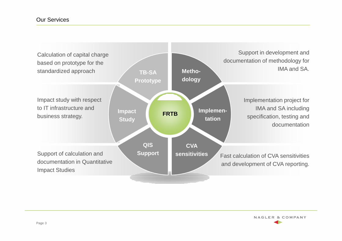
Our Services

Page 3

Source: CP1/3

FRTB

Support in development and documentation of methodology for

IMA and SA.

Implementation project for IMA and SA including

specification, testing and documentation

Support of calculation and documentation in Quantitative Impact Studies

Calculation of capital charge based on prototype for the standardized approach

Impact study with respect to IT infrastructure and business strategy.

Fast calculation of CVA sensitivities and development of CVA reporting.

TB-SA Prototype

Impact Study

QIS Support

Metho-dology

Implemen-tation

CVA sensitivities

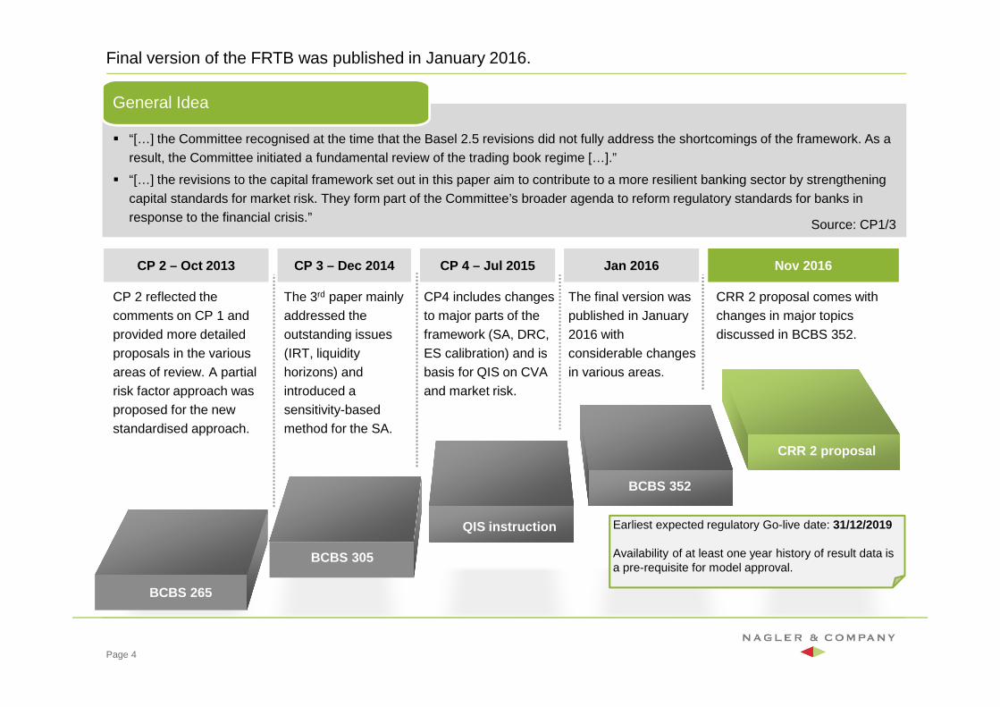
Final version of the FRTB was published in January 2016.

Page 4

� “[…] the Committee recognised at the time that the Basel 2.5 revisions did not fully address the shortcomings of the framework. As a result, the Committee initiated a fundamental review of the trading book regime […].”

� “[…] the revisions to the capital framework set out in this paper aim to contribute to a more resilient banking sector by strengthening capital standards for market risk. They form part of the Committee’s broader agenda to reform regulatory standards for banks in response to the financial crisis.”

General Idea

CP 2 – Oct 2013 CP 4 – Jul 2015 Nov 2016

CP 2 reflected the comments on CP 1 and provided more detailed proposals in the various areas of review. A partial risk factor approach was proposed for the new standardised approach.

CP 3 – Dec 2014 Jan 2016

BCBS 265

BCBS 305

QIS instruction

BCBS 352

CRR 2 proposal

The final version was published in January 2016 with considerable changes in various areas.

CRR 2 proposal comes with changes in major topics discussed in BCBS 352.

CP4 includes changes to major parts of the framework (SA, DRC, ES calibration) and is basis for QIS on CVA and market risk.

The 3rd paper mainly addressed the outstanding issues (IRT, liquidity horizons) and introduced a sensitivity-based method for the SA.

Source: CP1/3

Earliest expected regulatory Go-live date: 31/12/2019

Availability of at least one year history of result data is a pre-requisite for model approval.

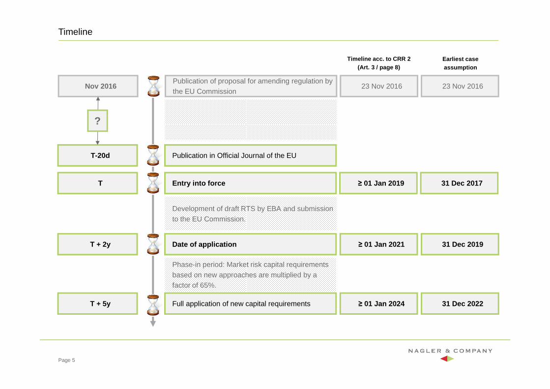
Timeline

Page 5

Nov 2016Publication of proposal for amending regulation by the EU Commission

T-20d Publication in Official Journal of the EU

T Entry into force

T + 2y Date of application

T + 5y Full application of new capital requirements

Development of draft RTS by EBA and submission to the EU Commission.

?

Phase-in period: Market risk capital requirements based on new approaches are multiplied by a factor of 65%.

23 Nov 2016 23 Nov 2016

≥ 01 Jan 2019 31 Dec 2017

≥ 01 Jan 2021 31 Dec 2019

≥ 01 Jan 2024 31 Dec 2022

Timeline acc. to CRR 2(Art. 3 / page 8)

Earliest case assumption

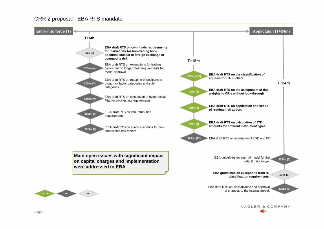
CRR 2 proposal - EBA RTS mandate

Page 6

Entry into force (T) Application (T+24m)

325 (8)

EBA draft RTS on own funds requirements for market risk for non-trading book positions subject to foreign exchange or commodity risk

325k (3)EBA draft RTS on the assignment of risk weights to CIUs without look-through

325v (5)EBA draft RTS on application and scope of residual risk addon.

325ba (4)EBA draft RTS on exemptions for trading desks that no longer meet requirements for model approval.

104a (1)EBA guidelines on exceptions from re-

classification requirements .

325x (8)EBA draft RTS on calculation of JTD amounts for different instrument types.

325aq (2-3)EBA draft RTS on the classification of equities for SA buckets.

325ba (8)EBA draft RTS on classification and approval

of changes to the internal model.

325be (7)EBA draft RTS on mapping of positions to broad risk factor categories and sub-categories. .

325bg (9)EBA draft RTS on calculation of hypotheticalP&L for backtesting requirements.

325bh (4)EBA draft RTS on P&L attribution requirements

325bk (4)EBA draft RTS on shock scenarios for non-modellable risk factors

325bn (3)EBA guidelines on internal model for the

default risk charge.

325bp (12) EBA draft RTS on estimation of LGD and PD

T+15m

T+6m

T+24m

Main open issues with significant impact on capital charges and implementation were addressed to EBA.

Page 7

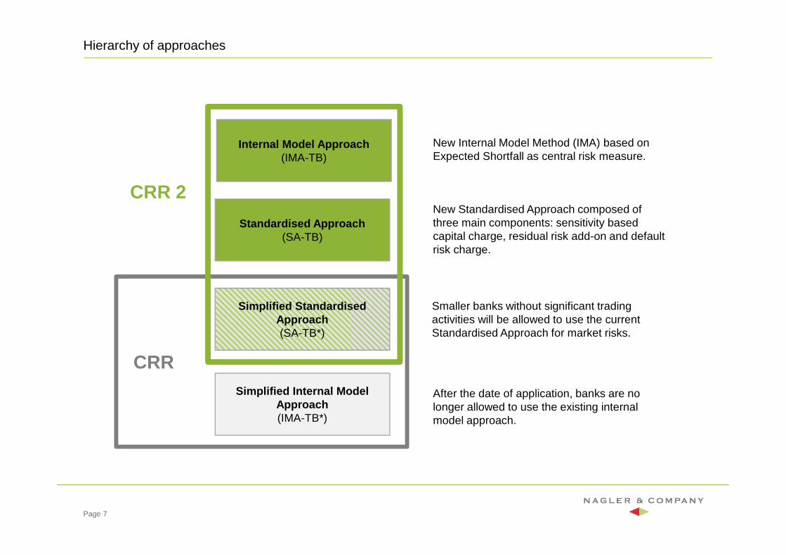
Hierarchy of approaches

Standardised Approach(SA-TB)

Internal Model Approach(IMA-TB)

Simplified StandardisedApproach(SA-TB*)

Simplified Internal Model Approach(IMA-TB*)

New Internal Model Method (IMA) based on Expected Shortfall as central risk measure.

New Standardised Approach composed of three main components: sensitivity based capital charge, residual risk add-on and default risk charge.

Smaller banks without significant trading activities will be allowed to use the current Standardised Approach for market risks.

After the date of application, banks are no longer allowed to use the existing internal model approach.

CRR

CRR 2

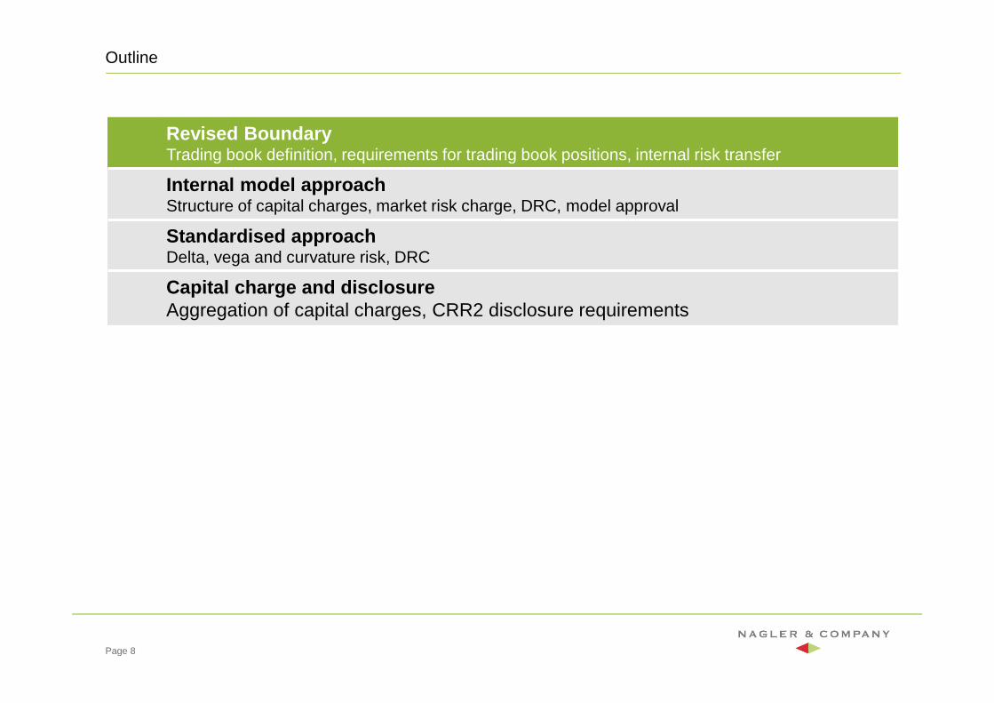
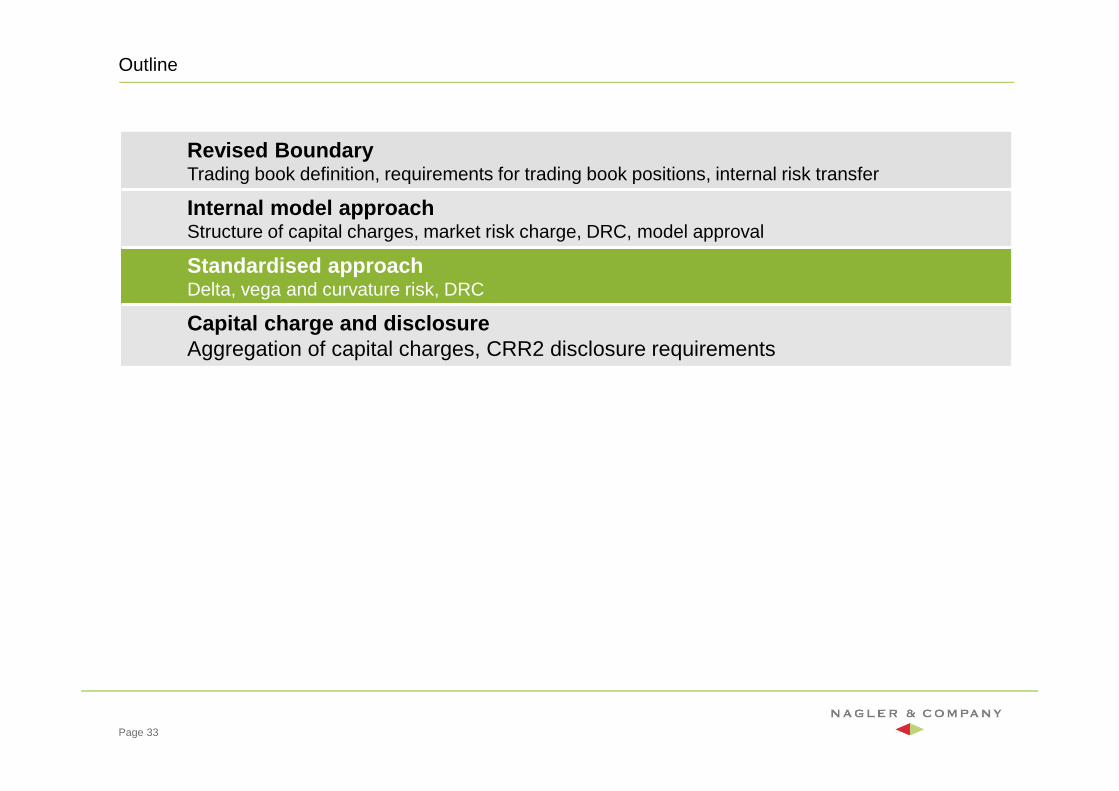
Outline

Page 8

Revised BoundaryTrading book definition, requirements for trading book positions, internal risk transfer

Internal model approachStructure of capital charges, market risk charge, DRC, model approval

Standardised approachDelta, vega and curvature risk, DRC

Capital charge and disclosureAggregation of capital charges, CRR2 disclosure requirements

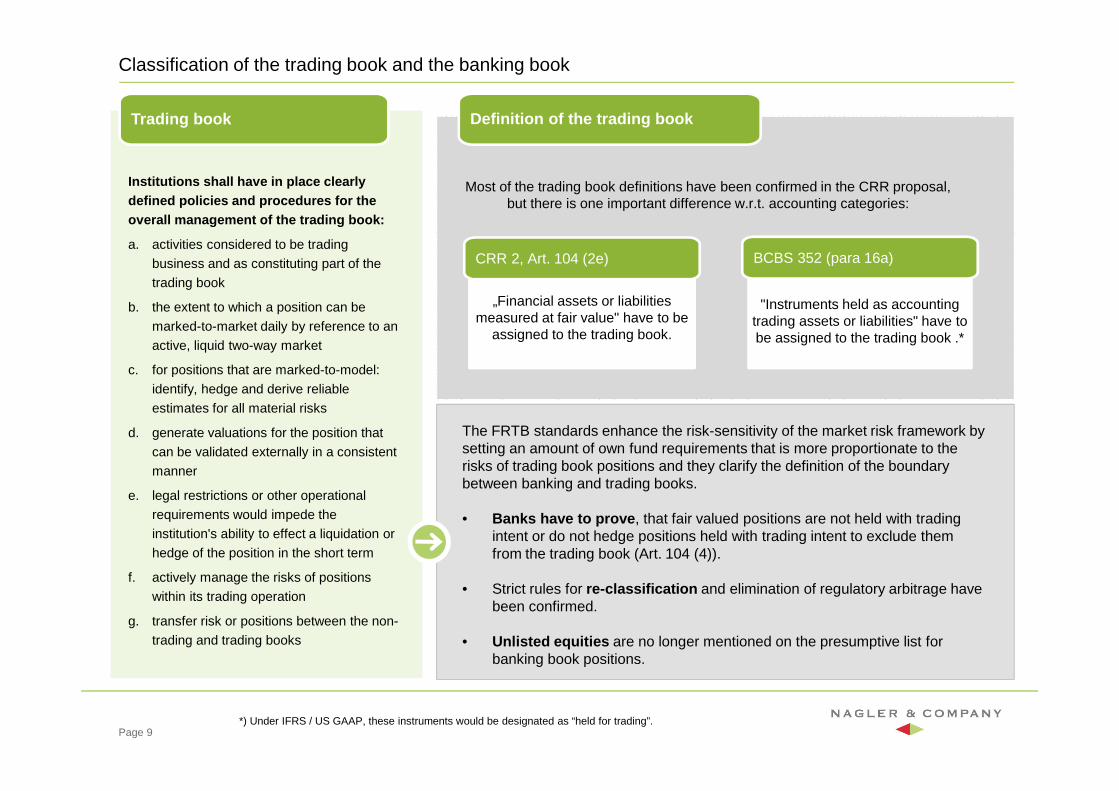
Classification of the trading book and the banking book

Page 9

"Instruments held as accounting trading assets or liabilities" have to be assigned to the trading book .*

„Financial assets or liabilities measured at fair value" have to be

assigned to the trading book.

*) Under IFRS / US GAAP, these instruments would be designated as “held for trading”.

Most of the trading book definitions have been confirmed in the CRR proposal, but there is one important difference w.r.t. accounting categories:

Trading book Definition of the trading book

CRR 2, Art. 104 (2e) BCBS 352 (para 16a)

The FRTB standards enhance the risk-sensitivity of the market risk framework by setting an amount of own fund requirements that is more proportionate to the risks of trading book positions and they clarify the definition of the boundary between banking and trading books.

• Banks have to prove , that fair valued positions are not held with trading intent or do not hedge positions held with trading intent to exclude them from the trading book (Art. 104 (4)).

• Strict rules for re-classification and elimination of regulatory arbitrage have been confirmed.

• Unlisted equities are no longer mentioned on the presumptive list for banking book positions.

Institutions shall have in place clearly defined policies and procedures for the overall management of the trading book:

a. activities considered to be trading

business and as constituting part of the

trading book

b. the extent to which a position can be

marked-to-market daily by reference to an

active, liquid two-way market

c. for positions that are marked-to-model:

identify, hedge and derive reliable

estimates for all material risks

d. generate valuations for the position that

can be validated externally in a consistent

manner

e. legal restrictions or other operational

requirements would impede the

institution's ability to effect a liquidation or

hedge of the position in the short term

f. actively manage the risks of positions

within its trading operation

g. transfer risk or positions between the non-

trading and trading books

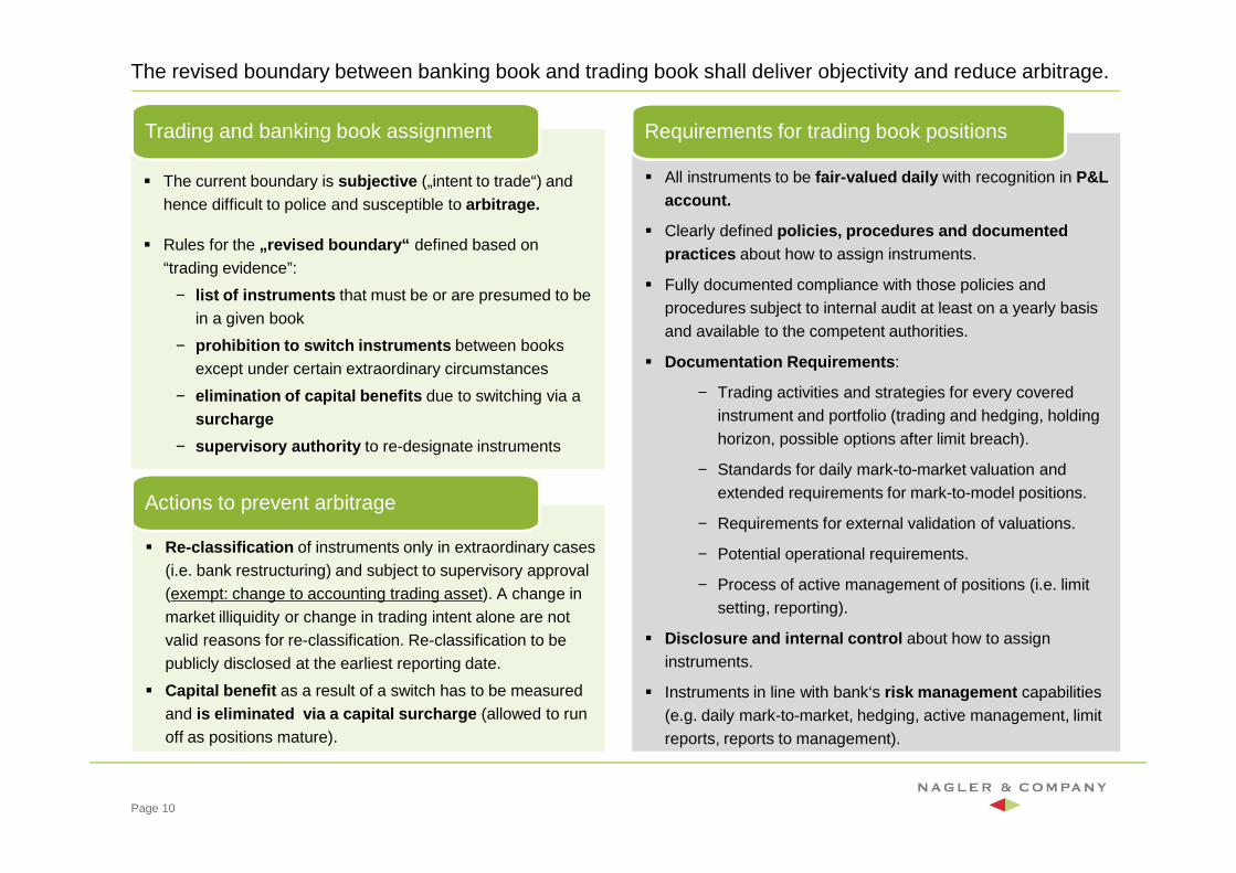
The revised boundary between banking book and trading book shall deliver objectivity and reduce arbitrage.

� The current boundary is subjective („intent to trade“) and hence difficult to police and susceptible to arbitrage.

� Rules for the „revised boundary“ defined based on “trading evidence”:

− list of instruments that must be or are presumed to be in a given book

− prohibition to switch instruments between books except under certain extraordinary circumstances

− elimination of capital benefits due to switching via a surcharge

− supervisory authority to re-designate instruments

Trading and banking book assignment

� All instruments to be fair-valued daily with recognition in P&L account.

� Clearly defined policies, procedures and documented practices about how to assign instruments.

� Fully documented compliance with those policies and procedures subject to internal audit at least on a yearly basis and available to the competent authorities.

� Documentation Requirements :

− Trading activities and strategies for every covered instrument and portfolio (trading and hedging, holding horizon, possible options after limit breach).

− Standards for daily mark-to-market valuation and extended requirements for mark-to-model positions.

− Requirements for external validation of valuations.

− Potential operational requirements.

− Process of active management of positions (i.e. limit setting, reporting).

� Disclosure and internal control about how to assign instruments.

� Instruments in line with bank‘s risk management capabilities (e.g. daily mark-to-market, hedging, active management, limit reports, reports to management).

Requirements for trading book positions

� Re-classification of instruments only in extraordinary cases (i.e. bank restructuring) and subject to supervisory approval (exempt: change to accounting trading asset). A change in market illiquidity or change in trading intent alone are not valid reasons for re-classification. Re-classification to be publicly disclosed at the earliest reporting date.

� Capital benefit as a result of a switch has to be measured and is eliminated via a capital surcharge (allowed to run off as positions mature).

Actions to prevent arbitrage

Page 10

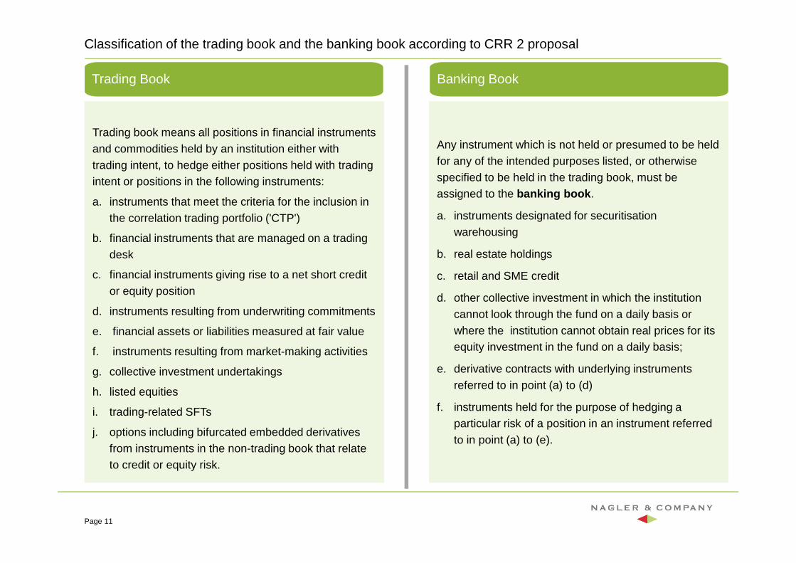
Classification of the trading book and the banking book according to CRR 2 proposal

Page 11

Trading Book Banking Book

Trading book means all positions in financial instruments and commodities held by an institution either with trading intent, to hedge either positions held with trading intent or positions in the following instruments:

a. instruments that meet the criteria for the inclusion in the correlation trading portfolio ('CTP')

b. financial instruments that are managed on a trading desk

c. financial instruments giving rise to a net short credit or equity position

d. instruments resulting from underwriting commitments

e. financial assets or liabilities measured at fair value

f. instruments resulting from market-making activities

g. collective investment undertakings

h. listed equities

i. trading-related SFTs

j. options including bifurcated embedded derivatives from instruments in the non-trading book that relate to credit or equity risk.

Any instrument which is not held or presumed to be held for any of the intended purposes listed, or otherwise specified to be held in the trading book, must be assigned to the banking book .

a. instruments designated for securitisationwarehousing

b. real estate holdings

c. retail and SME credit

d. other collective investment in which the institution cannot look through the fund on a daily basis or where the institution cannot obtain real prices for its equity investment in the fund on a daily basis;

e. derivative contracts with underlying instruments referred to in point (a) to (d)

f. instruments held for the purpose of hedging a particular risk of a position in an instrument referred to in point (a) to (e).

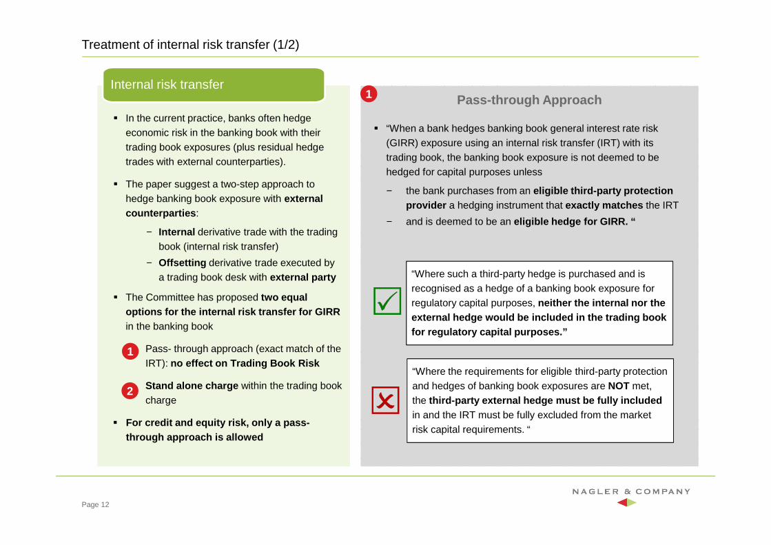
Treatment of internal risk transfer (1/2)

� In the current practice, banks often hedge economic risk in the banking book with their trading book exposures (plus residual hedge trades with external counterparties).

� The paper suggest a two-step approach to hedge banking book exposure with external counterparties :

− Internal derivative trade with the trading book (internal risk transfer)

− Offsetting derivative trade executed by a trading book desk with external party

� The Committee has proposed two equal options for the internal risk transfer for GIRRin the banking book

� Pass- through approach (exact match of the IRT): no effect on Trading Book Risk

� Stand alone charge within the trading book charge

� For credit and equity risk, only a pass-through approach is allowed

Internal risk transfer

Page 12

Pass-through Approach

1

2

1

� “When a bank hedges banking book general interest rate risk (GIRR) exposure using an internal risk transfer (IRT) with its trading book, the banking book exposure is not deemed to be hedged for capital purposes unless

− the bank purchases from an eligible third-party protection provider a hedging instrument that exactly matches the IRT

− and is deemed to be an eligible hedge for GIRR. “

“Where such a third-party hedge is purchased and is recognised as a hedge of a banking book exposure for regulatory capital purposes, neither the internal nor the external hedge would be included in the trading boo k for regulatory capital purposes.”

“Where the requirements for eligible third-party protection and hedges of banking book exposures are NOT met, the third-party external hedge must be fully included in and the IRT must be fully excluded from the market risk capital requirements. “

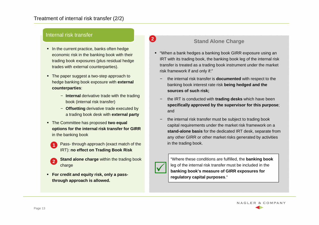
Treatment of internal risk transfer (2/2)

� In the current practice, banks often hedge economic risk in the banking book with their trading book exposures (plus residual hedge trades with external counterparties).

� The paper suggest a two-step approach to hedge banking book exposure with external counterparties :

− Internal derivative trade with the trading book (internal risk transfer)

− Offsetting derivative trade executed by a trading book desk with external party

� The Committee has proposed two equal options for the internal risk transfer for GIRRin the banking book

� Pass- through approach (exact match of the IRT): no effect on Trading Book Risk

� Stand alone charge within the trading book charge

� For credit and equity risk, only a pass-through approach is allowed.

Internal risk transfer

Page 13

Stand Alone Charge

2

2

� “When a bank hedges a banking book GIRR exposure using an IRT with its trading book, the banking book leg of the internal risk transfer is treated as a trading book instrument under the market risk framework if and only if:”

− the internal risk transfer is documented with respect to the banking book interest rate risk being hedged and the sources of such risk;

− the IRT is conducted with trading desks which have been specifically approved by the supervisor for this pu rpose ; and

− the internal risk transfer must be subject to trading book capital requirements under the market risk framework on a stand-alone basis for the dedicated IRT desk, separate from any other GIRR or other market risks generated by activities in the trading book.

“Where these conditions are fulfilled, the banking book leg of the internal risk transfer must be included in the banking book’s measure of GIRR exposures for regulatory capital purposes .“

1

Outline

Page 14





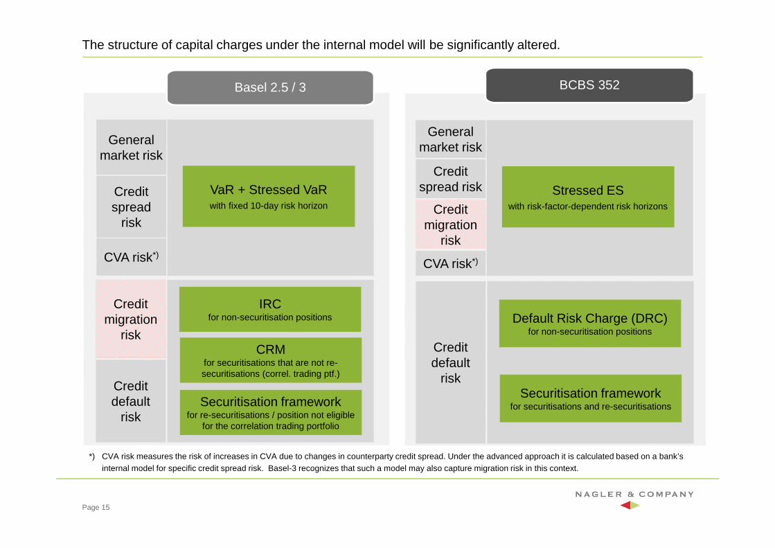
The structure of capital charges under the internal model will be significantly altered.

General market risk

Credit spread

risk

Basel 2.5 / 3 BCBS 352

VaR + Stressed VaRwith fixed 10-day risk horizon

CVA risk*)

IRCfor non-securitisation positions

CRMfor securitisations that are not re-securitisations (correl. trading ptf.)

Securitisation frameworkfor re-securitisations / position not eligible

for the correlation trading portfolio

Credit migration

risk

Credit default

risk

General market risk

Credit spread risk Stressed ES

with risk-factor-dependent risk horizons

CVA risk*)

Credit migration

risk

Default Risk Charge (DRC)for non-securitisation positions

Securitisation frameworkfor securitisations and re-securitisations

Credit default

risk

*) CVA risk measures the risk of increases in CVA due to changes in counterparty credit spread. Under the advanced approach it is calculated based on a bank’s internal model for specific credit spread risk. Basel-3 recognizes that such a model may also capture migration risk in this context.

Page 15

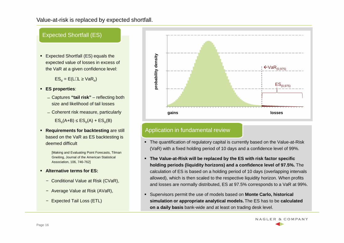
Value-at-risk is replaced by expected shortfall.

� Expected Shortfall (ES) equals the expected value of losses in excess of the VaR at a given confidence level:

ESα = E(LL ≥ VaRα)

� ES properties :

Captures “tail risk” – reflecting both size and likelihood of tail losses

Coherent risk measure, particularly

ESα(A+B) ≤ ESα(A) + ESα(B)

� Requirements for backtesting are still based on the VaR as ES backtesting is deemed difficult

[Making and Evaluating Point Forecasts, TilmanGneiting, Journal of the American Statistical Association, 106, 746-762]

� Alternative terms for ES:

− Conditional Value at Risk (CVaR),

− Average Value at Risk (AVaR),

− Expected Tail Loss (ETL)

0,0E+00

1,0E+05

2,0E+05

3,0E+05

4,0E+05

0 10 20 30 40 50 60 70 80 90 100

Expected Shortfall (ES)

� The quantification of regulatory capital is currently based on the Value-at-Risk (VaR) with a fixed holding period of 10 days and a confidence level of 99%.

� The Value-at-Risk will be replaced by the ES with r isk factor specific holding periods (liquidity horizons) and a confidenc e level of 97.5%. The calculation of ES is based on a holding period of 10 days (overlapping intervals allowed), which is then scaled to the respective liquidity horizon. When profits and losses are normally distributed, ES at 97.5% corresponds to a VaR at 99%.

� Supervisors permit the use of models based on Monte Carlo, historical simulation or appropriate analytical models. The ES has to be calculated on a daily basis bank-wide and at least on trading desk level.

Application in fundamental review

�VaR(0,975)

ES(0,975)

gains losses

prob

abili

tyde

nsity

Page 16

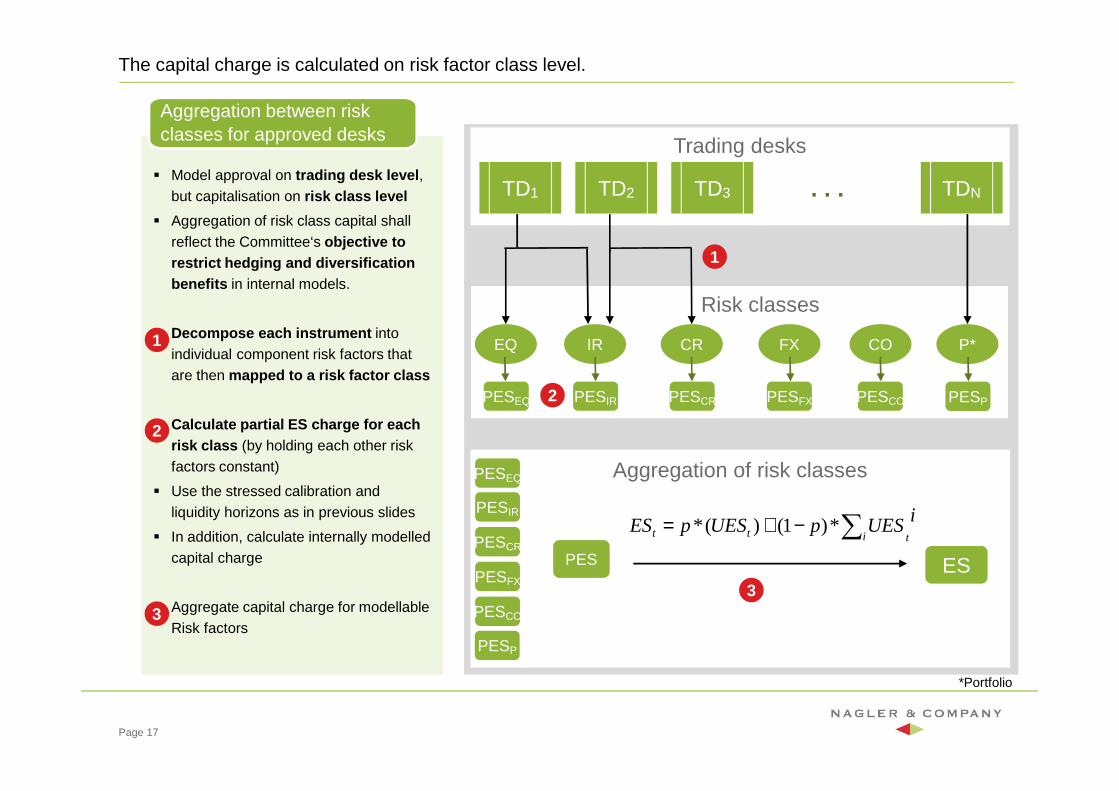
The capital charge is calculated on risk factor class level.

� Model approval on trading desk level , but capitalisation on risk class level

� Aggregation of risk class capital shall reflect the Committee‘s objective to restrict hedging and diversification benefits in internal models.

� Decompose each instrument into individual component risk factors that are then mapped to a risk factor class

� Calculate partial ES charge for each risk class (by holding each other risk factors constant)

� Use the stressed calibration and liquidity horizons as in previous slides

� In addition, calculate internally modelled capital charge

� Aggregate capital charge for modellableRisk factors

Aggregation between risk classes for approved desks

Trading desks

TD1 TD2 TDNTD3 . . .

Risk classes

Aggregation of risk classes

ES

PESEQ

PESIR

PESCR

PESFX

PESCO

EQ

PESEQ

IR

PESIR

CR

PESCR

FX

PESFX

CO

PESCO

1

3

PES

1

2

3

Page 17

P*

PESP2

PESP

*Portfolio

iUESpUESpEStitt ∑−+= *)1()(*

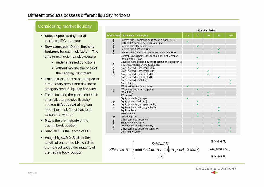
Different products possess different liquidity horizons.

� Status Quo: 10 days for all products; IRC: one year

� New approach : Define liquidity horizons for each risk factor = The time to extinguish a risk exposure

� under stressed conditions

� without moving the price of the hedging instrument

� Each risk factor must be mapped to a regulatory prescribed risk factor category resp. 5 liquidity horizons.

� For calculating the partial expected shortfall, the effective liquidity horizon EffectiveLH of a given modellable risk factor has to be calculated, where:

� Mat is the the maturity of the trading book position;

� SubCatLH is the length of LH;

� �� {��/�� ≥ �� } is the

length of one of the LH, which is the nearest above the maturity of the trading book position

Considering market liquidity

Page 18

Liquidity Horizon

Risk Class Risk Factor Category 10 20 40 60 120

Inte

rest

Rat

e Interest rate – domestic currency of a bank: EUR, USD, GBP, AUD, JPY, SEK, and CAD

✔

Interest rate other currencies ✔

Interest rate ATM volatility ✔

Interest rate (other than yields and ATM volatility) ✔

Cre

dit R

isk

Central Government, incl. central banks of Member States of the Union

✔

Covered bonds issued by credit institutions established in Member States of the Union (IG)

✔

Credit spread – sovereign (IG) ✔

Credit spread – sovereign (HY) ✔

Credit spread – corporate(IG) ✔

Credit spread – corporate(HY) ✔

Credit spread – volatility ✔

Credit (other) ✔

FX

FX rate-liquid currency pairs ✔

FX rate (other currency pairs) ✔

FX volatility ✔

FX (other) ✔

Equ

ity

Equity price (large cap) ✔

Equity price (small cap) ✔

Equity price (large cap) volatility ✔

Equity price (small cap) volatility ✔

Equity (other) ✔

Com

mod

ityEnergy price ✔

Precious price ✔

Other commodities price ✔

Energy price volatility ✔

Precious metal price volatility ✔

Other commodities price volatility ✔

Commodity (other) ✔

{ })/min,min(

1

Mat

LH

LHLHSubCatLH

SubCatLH

HEffectiveL jjj

≥

=

If Mat>��If ��≤Mat≤��

If Mat<��

General requirements when using internal models

Calculation Steps:

• Risk measure �� for any given t

• �� is the unconstrained expected shortfall measure for broad risk

factor category. We calculate �� for broad risk factor category i

• Daily calculations of the partial expected shortfall numbers. With 97,5%, one tail confidence interval

• When calculating the partial

expected shortfall �� and �� ,

the scenarios of future shocks shall only be applied to the subset of modellable risk factors of positions.

For calculating �� , the scenarios

shall be applied to all the modellablerisk factors.

• Scaling of ES to the liquidity horizon of a risk factor according to specified horizons from the Committee (assignment from 10d to 1y). Only relevant risk factors will be shifted.

ES risk measure

i is the index of the five broad risk factor categories (IR, EQ, CS, COM, FX)

p is supervisory correlation factor across broad risk categories; p=50%

For a given portfolio of trading book positions, the partial expected shortfall number �� at time t is calculated as follows:

j is the index of the five liquidity horizons

�� is the length of liquidity horizons j

T =10 days

Page 19

1

2

EST ES

3 4

2

2

12

10),())(( ∑

≥

−

−+=

j

jjttt

LHLHjTPESTPESPES

iUESpUESpEStitt ∑⋅−+⋅= )1()(1

= 1,max RC

t

FCtRS

ttPES

PESPESUES o2

3

Scaling to liquidity horizon

4

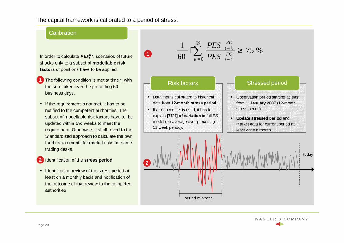
The capital framework is calibrated to a period of stress.

In order to calculate �� , scenarios of future

shocks only to a subset of modellable risk factors of positions have to be applied:

� The following condition is met at time t, with the sum taken over the preceding 60 business days.

� If the requirement is not met, it has to be notified to the competent authorities. The subset of modellable risk factors have to be updated within two weeks to meet the requirement. Otherwise, it shall revert to the Standardized approach to calculate the own fund requirements for market risks for some trading desks.

� Identification of the stress period

� Identification review of the stress period at least on a monthly basis and notification of the outcome of that review to the competent authorities

Calibration

period of stress

today

2

� Data inputs calibrated to historical

data from 12-month stress period

� If a reduced set is used, it has to

explain [75%] of variation in full ES

model (on average over preceding

12 week period).

Risk factors

� Observation period starting at least

from 1. January 2007 (12-month

stress perios)

� Update stressed period and

market data for current period at

least once a month.

Stressed period1

2

Page 20

1 %7560

1 59

0

≥⋅∑= −

−

kFC

kt

RCkt

PES

PES

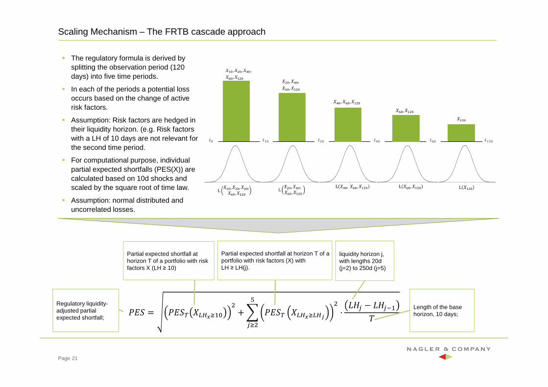
Scaling Mechanism – The FRTB cascade approach

Page 21

� The regulatory formula is derived by splitting the observation period (120 days) into five time periods.

� In each of the periods a potential loss occurs based on the change of active risk factors.

� Assumption: Risk factors are hedged in their liquidity horizon. (e.g. Risk factors with a LH of 10 days are not relevant for the second time period.

� For computational purpose, individual partial expected shortfalls (PES(X)) are calculated based on 10d shocks and scaled by the square root of time law.

� Assumption: normal distributed and uncorrelated losses.

�� = �� !"#$ + & �� !��'

$ ⋅)

*!$+,* − +,*."/

Regulatory liquidity-adjusted partial expected shortfall;

liquidity horizon j, with lengths 20d (j=2) to 250d (j=5)

Length of the base horizon, 10 days;

Partial expected shortfall at horizon T of a portfolio with risk factors X (LH ≥ 10)

Partial expected shortfall at horizon T of a portfolio with risk factors (X) with LH ≥ LH(j).

Multiple runs needed to produce required PES results.

� A run is a historical simulation in which a subset of risk factors is subject to historical shifts where all other risk factors are kept constant.

� This includes in particular 254 revaluations.

� 21 runs possible to cover LH and Risk Factor combinations :

� 3 runs for Standalone PESFX

� 3 runs for Standalone PESIR

� 4 runs for Standalone PESCR

� 3 runs for Standalone PESEQ

� 3 runs for Standalone PESCO

� 5 runs for PESAll

� 3 combinations of market data and risk factor universes to be used (indirect method):

� Stressed data / reduced set of risk factors

� Current data / reduced set of risk factors

� Current data / full set of risk factors (monthly)

� 63 runs possible to generate all required HistSim vectors on desk level.

� LH overrides per desk and the use of reduced set of risk factors could increase the number.

Calculation of HistSimvectors

Page 22

Overall up to 63 runs are possibly needed to genera te all required results for the PES calculation.

Additional runs needed for identification of Stress Period and production of data for Backtesting.

10 20 40 60 120

IR

CS

EQ

FX

COM

All

Liquidity horizon

Ris

kfa

ctor

cate

gory

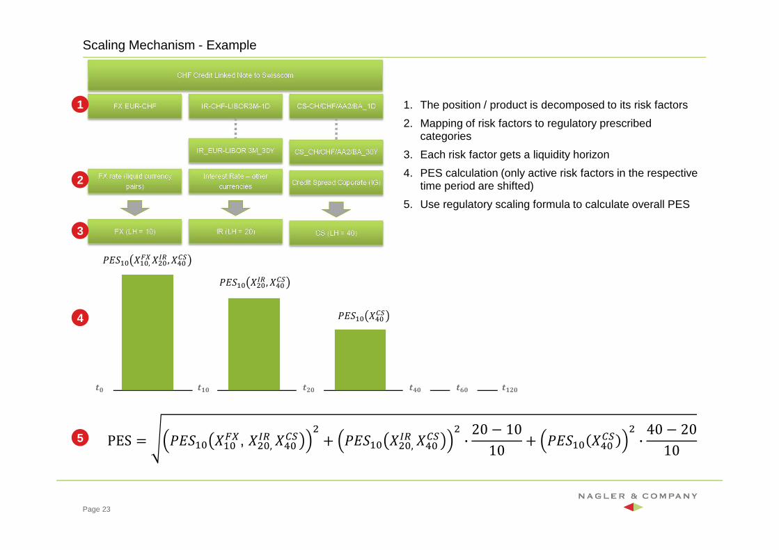
Scaling Mechanism - Example

Page 23

PES = ��"# �"#34, �$#, 67 �8#9: $ + ��"# �$#, 67 �8#9: $ · 20 − 1010 + ��"# �8#9: $ · 40 − 20

10

1. The position / product is decomposed to its risk factors

2. Mapping of risk factors to regulatory prescribed categories

3. Each risk factor gets a liquidity horizon

4. PES calculation (only active risk factors in the respective time period are shifted)

5. Use regulatory scaling formula to calculate overall PES

1

3

2

4

5

��"# �"#, 34 �$#67 , �8#9:

��"# �$#67 , �8#9:

��"# �8#9:

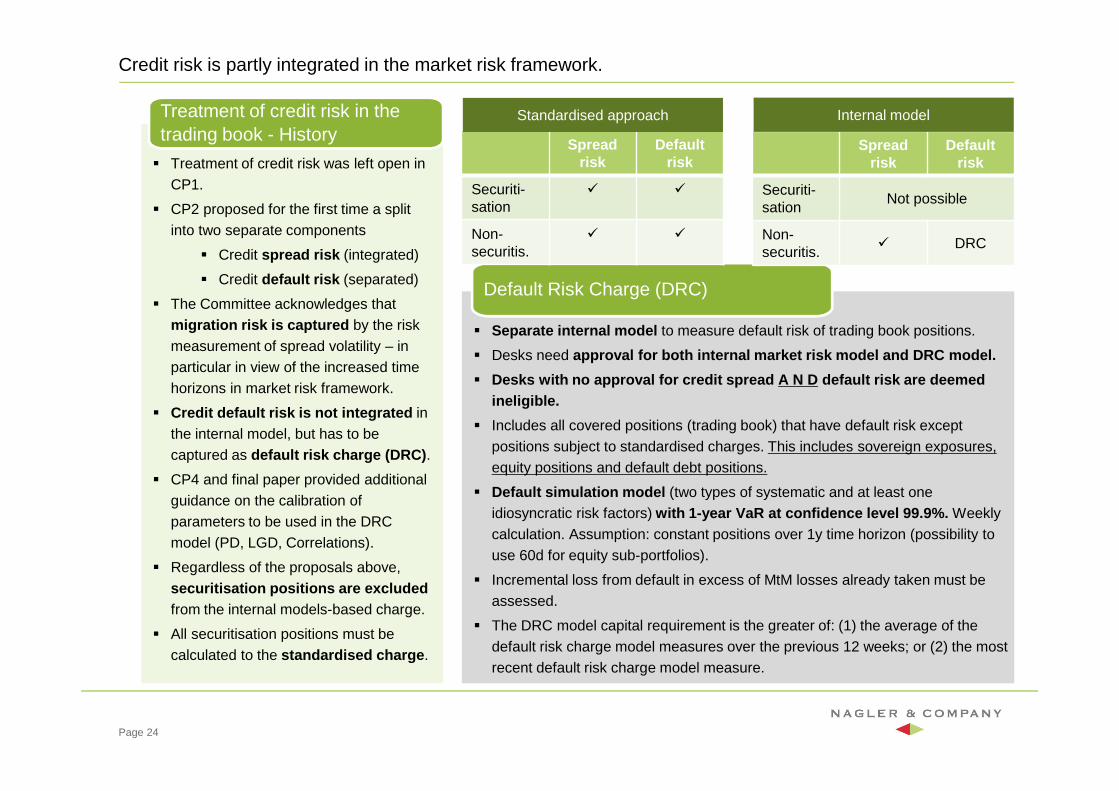
Credit risk is partly integrated in the market risk framework.

� Treatment of credit risk was left open in CP1.

� CP2 proposed for the first time a split into two separate components

� Credit spread risk (integrated)

� Credit default risk (separated)

� The Committee acknowledges that migration risk is captured by the risk measurement of spread volatility – in particular in view of the increased time horizons in market risk framework.

� Credit default risk is not integrated in the internal model, but has to be captured as default risk charge (DRC) .

� CP4 and final paper provided additional guidance on the calibration of parameters to be used in the DRC model (PD, LGD, Correlations).

� Regardless of the proposals above, securitisation positions are excluded from the internal models-based charge.

� All securitisation positions must be calculated to the standardised charge .

Treatment of credit risk in the trading book - History

� Separate internal model to measure default risk of trading book positions.

� Desks need approval for both internal market risk model and DR C model.

� Desks with no approval for credit spread A N D defau lt risk are deemed ineligible.

� Includes all covered positions (trading book) that have default risk except positions subject to standardised charges. This includes sovereign exposures, equity positions and default debt positions.

� Default simulation model (two types of systematic and at least one idiosyncratic risk factors) with 1-year VaR at confidence level 99.9%. Weekly calculation. Assumption: constant positions over 1y time horizon (possibility to use 60d for equity sub-portfolios).

� Incremental loss from default in excess of MtM losses already taken must be assessed.

� The DRC model capital requirement is the greater of: (1) the average of the default risk charge model measures over the previous 12 weeks; or (2) the most recent default risk charge model measure.

Default Risk Charge (DRC)

Spread risk

Default risk

Securiti-sation

� �

Non-securitis.

� �

Spread risk

Default risk

Securiti-sation

Not possible

Non-securitis.

� DRC

Standardised approach Internal model

Page 24

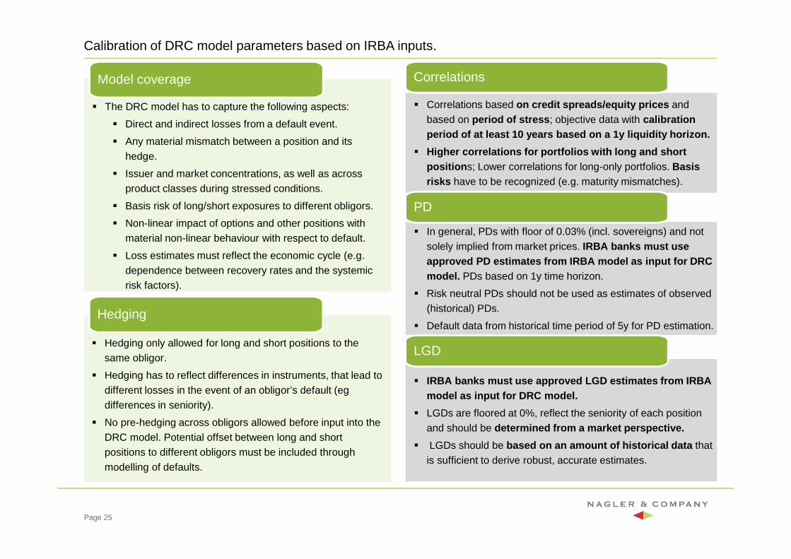
Calibration of DRC model parameters based on IRBA inputs.

� The DRC model has to capture the following aspects:

� Direct and indirect losses from a default event.

� Any material mismatch between a position and its hedge.

� Issuer and market concentrations, as well as across product classes during stressed conditions.

� Basis risk of long/short exposures to different obligors.

� Non-linear impact of options and other positions with material non-linear behaviour with respect to default.

� Loss estimates must reflect the economic cycle (e.g. dependence between recovery rates and the systemic risk factors).

Model coverage

� Correlations based on credit spreads/equity prices and based on period of stress ; objective data with calibration period of at least 10 years based on a 1y liquidity horizon.

� Higher correlations for portfolios with long and sh ort position s; Lower correlations for long-only portfolios. Basis risks have to be recognized (e.g. maturity mismatches).

Correlations

Page 25

� Hedging only allowed for long and short positions to the same obligor.

� Hedging has to reflect differences in instruments, that lead to different losses in the event of an obligor’s default (egdifferences in seniority).

� No pre-hedging across obligors allowed before input into the DRC model. Potential offset between long and short positions to different obligors must be included through modelling of defaults.

Hedging

� In general, PDs with floor of 0.03% (incl. sovereigns) and not solely implied from market prices. IRBA banks must use approved PD estimates from IRBA model as input for DRC model. PDs based on 1y time horizon.

� Risk neutral PDs should not be used as estimates of observed (historical) PDs.

� Default data from historical time period of 5y for PD estimation.

PD

� IRBA banks must use approved LGD estimates from IRB A model as input for DRC model.

� LGDs are floored at 0%, reflect the seniority of each position and should be determined from a market perspective.

� LGDs should be based on an amount of historical data that is sufficient to derive robust, accurate estimates.

LGD

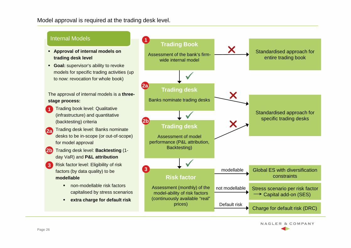
Model approval is required at the trading desk level.

Trading Book

Assessment of the bank‘s firm-wide internal model

Trading desk

Banks nominate trading desks

Standardised approach for entire trading book

Standardised approach for specific trading desks

Global ES with diversification constraints

Charge for default risk (DRC)

modellable

not modellable Stress scenario per risk factorCapital add-on (SES)

�

�

�

�

Risk factor

Assessment (monthly) of the model-ability of risk factors

(continuously available “real” prices) Default risk

� Approval of internal models on trading desk level

� Goal: supervisor‘s ability to revoke models for specific trading activities (up to now: revocation for whole book)

The approval of internal models is a three-stage process:

� Trading book level: Qualitative (infrastructure) and quantitative (backtesting) criteria

� Trading desk level: Banks nominate desks to be in-scope (or out-of-scope) for model approval

� Trading desk level: Backtesting (1-day VaR) and P&L attribution

� Risk factor level: Eligibility of risk factors (by data quality) to be modellable

� non-modellable risk factors capitalised by stress scenarios

� extra charge for default risk

Internal Models

Trading desk

Assessment of model performance (P&L attribution,

Backtesting)

��

Page 26

1

2a

3

2b

1

2a

2b

3

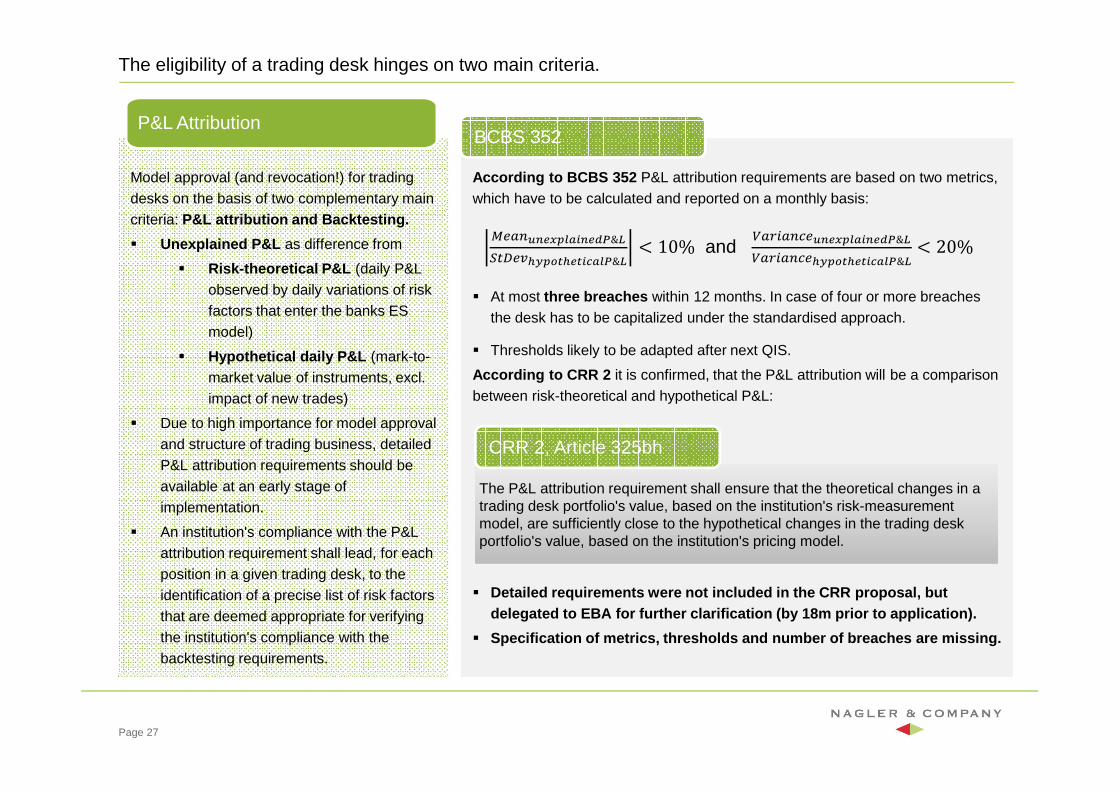
The eligibility of a trading desk hinges on two main criteria.

Model approval (and revocation!) for trading desks on the basis of two complementary main criteria: P&L attribution and Backtesting.

� Unexplained P&L as difference from

� Risk-theoretical P&L (daily P&L observed by daily variations of risk factors that enter the banks ES model)

� Hypothetical daily P&L (mark-to-market value of instruments, excl. impact of new trades)

� Due to high importance for model approval and structure of trading business, detailed P&L attribution requirements should be available at an early stage of implementation.

� An institution's compliance with the P&L attribution requirement shall lead, for each position in a given trading desk, to the identification of a precise list of risk factors that are deemed appropriate for verifying the institution's compliance with the backtesting requirements.

P&L Attribution

According to BCBS 352 P&L attribution requirements are based on two metrics, which have to be calculated and reported on a monthly basis:

� At most three breaches within 12 months. In case of four or more breaches the desk has to be capitalized under the standardised approach.

� Thresholds likely to be adapted after next QIS.

According to CRR 2 it is confirmed, that the P&L attribution will be a comparison between risk-theoretical and hypothetical P&L:

� Detailed requirements were not included in the CRR proposal, but delegated to EBA for further clarification (by 18m prior to application).

� Specification of metrics, thresholds and number of breaches are missing.

Page 27

@ABCDEF GHIJEFKL&N:OPAQRSGTURFUJVIHL&N < 10% and

YBZ[BC\ADEF GHIJEFKL&NYBZ[BC\ARSGTURFUJVIHL&N < 20%

The P&L attribution requirement shall ensure that the theoretical changes in a trading desk portfolio's value, based on the institution's risk-measurement model, are sufficiently close to the hypothetical changes in the trading desk portfolio's value, based on the institution's pricing model.

The P&L attribution requirement shall ensure that the theoretical changes in a trading desk portfolio's value, based on the institution's risk-measurement model, are sufficiently close to the hypothetical changes in the trading desk portfolio's value, based on the institution's pricing model.

CRR 2, Article 325bh

BCBS 352

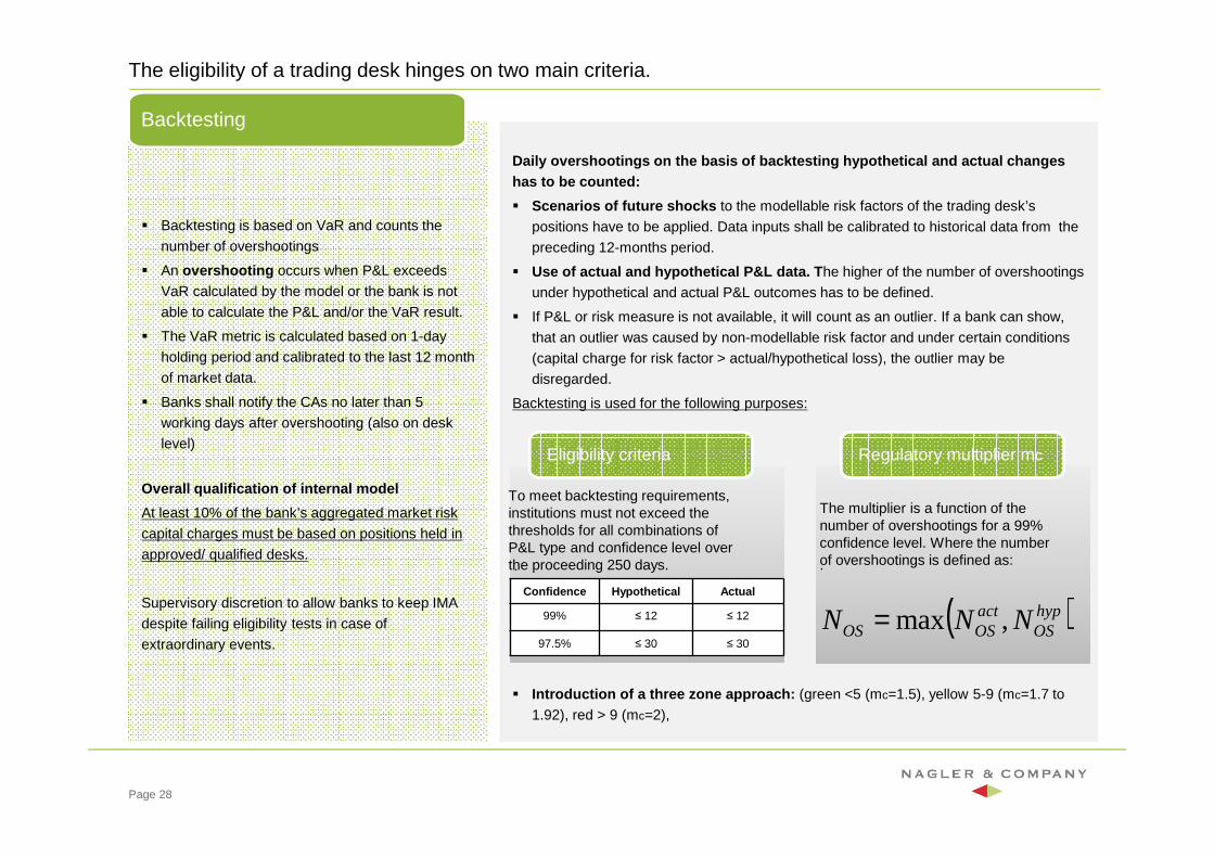
The eligibility of a trading desk hinges on two main criteria.

� Backtesting is based on VaR and counts the

number of overshootings

� An overshooting occurs when P&L exceeds

VaR calculated by the model or the bank is not

able to calculate the P&L and/or the VaR result.

� The VaR metric is calculated based on 1-day

holding period and calibrated to the last 12 month

of market data.

� Banks shall notify the CAs no later than 5

working days after overshooting (also on desk

level)

Overall qualification of internal model

At least 10% of the bank’s aggregated market risk

capital charges must be based on positions held in

approved/ qualified desks.

Supervisory discretion to allow banks to keep IMA

despite failing eligibility tests in case of

extraordinary events.

Backtesting

Daily overshootings on the basis of backtesting hypot hetical and actual changes has to be counted:

� Scenarios of future shocks to the modellable risk factors of the trading desk’s

positions have to be applied. Data inputs shall be calibrated to historical data from the

preceding 12-months period.

� Use of actual and hypothetical P&L data. T he higher of the number of overshootings

under hypothetical and actual P&L outcomes has to be defined.

� If P&L or risk measure is not available, it will count as an outlier. If a bank can show,

that an outlier was caused by non-modellable risk factor and under certain conditions

(capital charge for risk factor > actual/hypothetical loss), the outlier may be

disregarded.

Backtesting is used for the following purposes:

� Introduction of a three zone approach: (green <5 (mc=1.5), yellow 5-9 (mc=1.7 to

1.92), red > 9 (mc=2),

Page 28

..

Confidence Hypothetical Actual

99% ≤ 12 ≤ 12

97.5% ≤ 30 ≤ 30

..

To meet backtesting requirements, institutions must not exceed the thresholds for all combinations of P&L type and confidence level over the proceeding 250 days.

Eligibility criteria Regulatory multiplier mc

The multiplier is a function of the number of overshootings for a 99% confidence level. Where the number of overshootings is defined as:

( )hypOS

actOSOS NNN ,max=

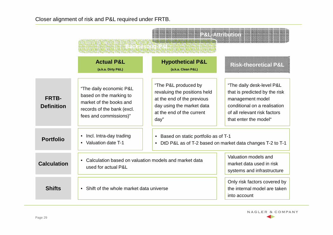
Closer alignment of risk and P&L required under FRTB.

Page 29

P&L-Attribution

Hypothetical P&L(a.k.a. Clean P&L)

“The P&L produced by revaluing the positions held at the end of the previous day using the market data at the end of the current day”

FRTB-Definition

Calculation• Calculation based on valuation models and market data

used for actual P&L

Valuation models and market data used in risk systems and infrastructure

Backtesting-P&L

Shifts • Shift of the whole market data universeOnly risk factors covered by the internal model are taken into account

Actual P&L(a.k.a. Dirty P&L)

“The daily economic P&L based on the marking to market of the books and records of the bank (excl. fees and commissions)”

Risk-theoretical P&L

“The daily desk-level P&L that is predicted by the risk management model conditional on a realisationof all relevant risk factors that enter the model“

Portfolio• Incl. Intra-day trading• Valuation date T-1

• Based on static portfolio as of T-1• DtD P&L as of T-2 based on market data changes T-2 to T-1

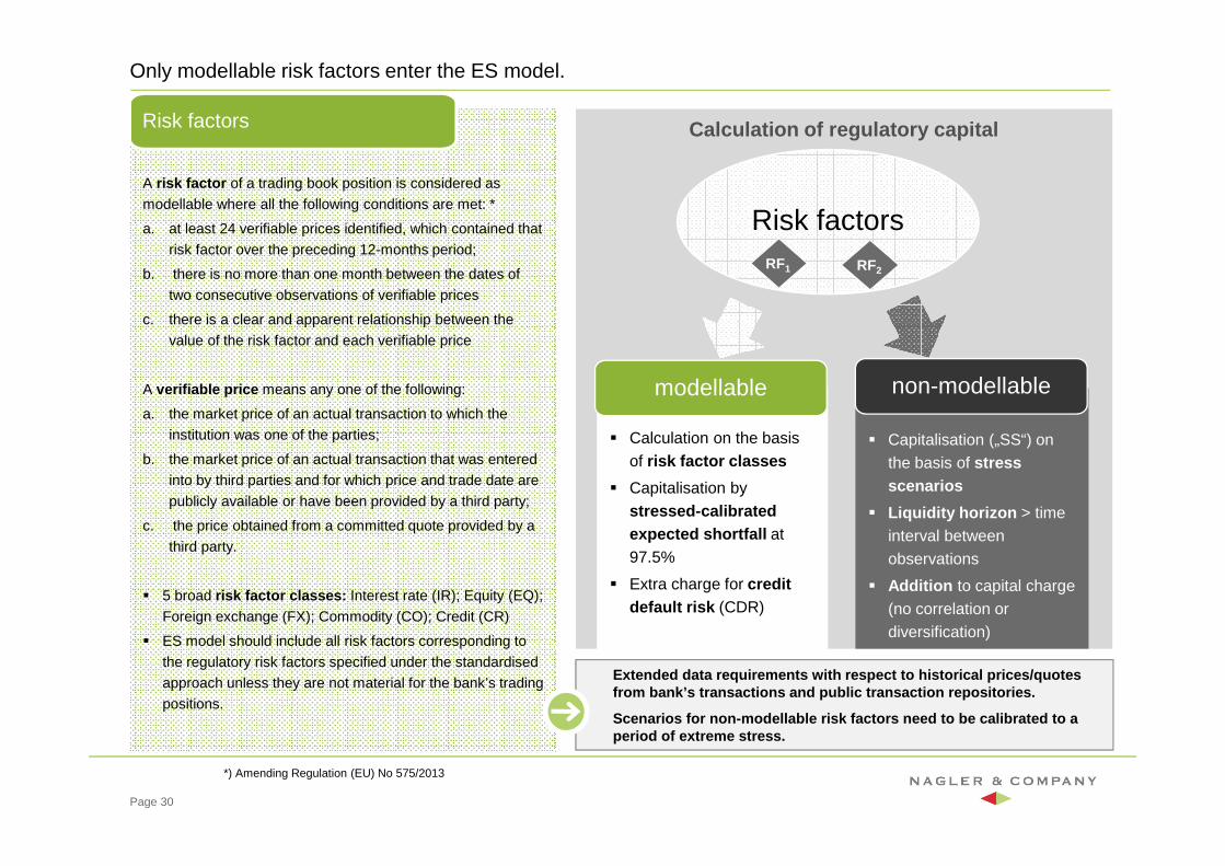
Only modellable risk factors enter the ES model.

Calculation of regulatory capital

� Calculation on the basis of risk factor classes

� Capitalisation by stressed-calibrated expected shortfall at 97.5%

� Extra charge for credit default risk (CDR)

Risk factors

� Capitalisation („SS“) on the basis of stress scenarios

� Liquidity horizon > time interval between observations

� Addition to capital charge (no correlation or diversification)

non-modellablemodellable

A risk factor of a trading book position is considered as

modellable where all the following conditions are met: *

a. at least 24 verifiable prices identified, which contained that

risk factor over the preceding 12-months period;

b. there is no more than one month between the dates of

two consecutive observations of verifiable prices

c. there is a clear and apparent relationship between the

value of the risk factor and each verifiable price

A verifiable price means any one of the following:

a. the market price of an actual transaction to which the

institution was one of the parties;

b. the market price of an actual transaction that was entered

into by third parties and for which price and trade date are

publicly available or have been provided by a third party;

c. the price obtained from a committed quote provided by a

third party.

� 5 broad risk factor classes: Interest rate (IR); Equity (EQ);

Foreign exchange (FX); Commodity (CO); Credit (CR)

� ES model should include all risk factors corresponding to

the regulatory risk factors specified under the standardised

approach unless they are not material for the bank’s trading

positions.

Risk factors

RF2RF1

Page 30

Extended data requirements with respect to historic al prices/quotes from bank’s transactions and public transaction rep ositories.

Scenarios for non-modellable risk factors need to be calibrated to a period of extreme stress.

*) Amending Regulation (EU) No 575/2013

Identification and capitalisation of Non-Modellable Risk Factors (NMRF) *

� According to BCBC 352, the risk factors are

defined as a principal determinant of the change

in value of a transaction that is used for the

quantification of risks’.

� The modellability is linked to an ability to observe

price data of sufficient quality and frequency, as

well as to the liquidity of instruments linked to the

specific risk factors.

� Hence, the new risk factors will always

be considered non-modellable, as not

enough transaction data is available for

the last year.

� The NMRF identification process is focused on

objectively validating risk factor values based on

real transactions.

� All risk factors identified as non modellable

according to the definition from the previous slide

must be capitalised individually, on a bank level

and based on stress scenarios for each NMRF,

taking into account the liquidity horizons.

Non-Modellable Risk Factor

Page 31

Calculation of price impact of the risk factor

•Retrieve the universe of relevant risk factors from all trading book positions

•Justify and document any risk factors omitted from IMA

Identify relevant risk factors

•Create mapping rules for identified risk factors to a set of instruments

•Risk factors can be evidence by more than one product

Create product mapping

•Retrieve vendor and internal bank transactions data and map back to risk factors using set of mapped instruments from step 2

Observability check

A material change in the value of a material risk factor should lead to a material change in the value of the transaction. The price impact for risk factor Is calculated as:

where is the sensitivity of the instrument with respect to risk factor ,and is the volatility of 10-day absolute changes for .

ii

i rfrf

PVrfPV σ*)(

∂∂=∆

)( irfPV∆ irf

irfPV ∂∂ / irfirfσ irf

Identification process for NMRF

*) based on Montoro, Becker, Popken (2017): “Identification and capitalization of non-modellable risk factors”, risk.net, February 2017)

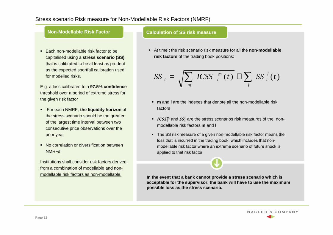
Stress scenario Risk measure for Non-Modellable Risk Factors (NMRF)

Non-Modellable Risk Factor

Page 32

)()( tSStICSSSSl

lt

m

mtt ∑∑ +=

� Each non-modellable risk factor to be capitalised using a stress scenario (SS) that is calibrated to be at least as prudent as the expected shortfall calibration used for modelled risks.

E.g. a loss calibrated to a 97.5% confidencethreshold over a period of extreme stress for the given risk factor

� For each NMRF, the liquidity horizon of the stress scenario should be the greater of the largest time interval between two consecutive price observations over the prior year

� No correlation or diversification between NMRFs

Institutions shall consider risk factors derived from a combination of modellable and non-modellable risk factors as non-modellable.

� At time t the risk scenario risk measure for all the non-modellablerisk factors of the trading book positions:

� m and l are the indexes that denote all the non-modellable risk factors

� ]�� and �� are the stress scenarios risk measures of the non-

modellable risk factors m and l

� The SS risk measure of a given non-modellable risk factor means the loss that is incurred in the trading book, which includes that non-modellable risk factor where an extreme scenario of future shock is applied to that risk factor.

Calculation of SS risk measure

In the event that a bank cannot provide a stress sc enario which is acceptable for the supervisor, the bank will have t o use the maximum possible loss as the stress scenario.

Outline

Page 33





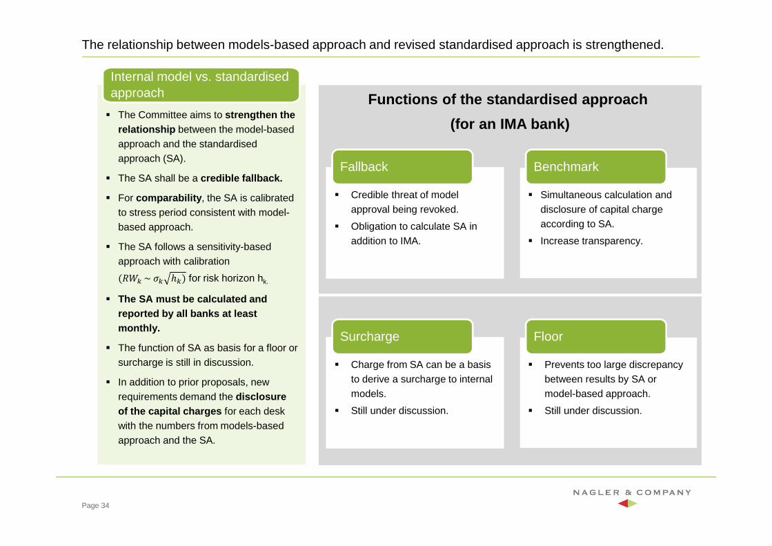
The relationship between models-based approach and revised standardised approach is strengthened.

� The Committee aims to strengthen the relationship between the model-based approach and the standardised approach (SA).

� The SA shall be a credible fallback.

� For comparability , the SA is calibrated to stress period consistent with model-based approach.

� The SA follows a sensitivity-based approach with calibration

(àb ~ db ℎb) for risk horizon hk.

� The SA must be calculated and reported by all banks at least monthly.

� The function of SA as basis for a floor or surcharge is still in discussion.

� In addition to prior proposals, new requirements demand the disclosure of the capital charges for each desk with the numbers from models-based approach and the SA.

Internal model vs. standardised approach Functions of the standardised approach

(for an IMA bank)

� Simultaneous calculation and disclosure of capital charge according to SA.

� Increase transparency.

Benchmark

� Credible threat of model approval being revoked.

� Obligation to calculate SA in addition to IMA.

Fallback

� Charge from SA can be a basis to derive a surcharge to internal models.

� Still under discussion.

Surcharge

� Prevents too large discrepancy between results by SA or model-based approach.

� Still under discussion.

Floor

Page 34

Risk Classes Instruments

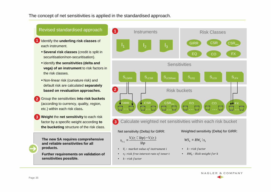
The concept of net sensitivities is applied in the standardised approach.

� Identify the underling risk classes of each instrument.

� Several risk classes (credit is split in securitisation/non-securitisation).

� Identify the sensitivities (delta and vega) of an instrument to risk factors in the risk classes.

� Non-linear risk (curvature risk) and default risk are calculated separately based on revaluation approaches.

� Group the sensitivities into risk buckets (according to currency, quality, region, etc.) within each risk class.

� Weight the net sensitivity to each risk factor by a specific weight according to the bucketing structure of the risk class.

Revised standardised approach

Page 35

1I2 I3I1

3

EQ

GIRR CSR

FXCO

CSRsec

1

SI,GIRR

Sensitivities

SI,GIRR SI,CSR SI,CSRsec SI,EQ SI,CO SI,FX

Risk buckets

GIRR

…CO

…FX

…

2

Calculate weighted net sensitivities within each risk bucket 3

bp

rVbprVs titi

rk t 1

)()1(,

−+=

Net sensitivity (Delta) for GIRR:

EQ

…CSR

…CSRsec

…

2

Weighted sensitivity (Delta) for GIRR:

• g ∶ ijkg lmnopi• àb ∶ `jkg qrjsℎo lpi g

• t[ ∶ umigro vmwxr pl jykoixuryo j• iO : ijkg lirr jyorirko imor pl orypi o• g ∶ ijkg lmnopi

The new SA requires comprehensive and reliable sensitivities for all products.

Further requirements on validation of sensitivities possible.

kkk sRWWS ⋅=

Cross risk class aggregation

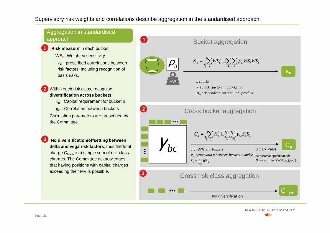
Supervisory risk weights and correlations describe aggregation in the standardised approach.

� Risk measure in each bucket

WSk : Weighted sensitivity

ρkl : prescribed correlations between risk factors. Including recognition of basis risks.

� Within each risk class, recognise diversification across buckets

Kb : Capital requirement for bucket b

γbc : Correlation between buckets

Correlation parameters are prescribed by the Committee.

� No diversification/offsetting between delta and vega risk factors , thus the total charge Clinear is a simple sum of risk class charges. The Committee acknowledges that having positions with capital charges exceeding their MV is possible.

Aggregation in standardised approach

Cross bucket aggregation

Bucket aggregation

RW

Kb

bcγ Ca

ijρ

Clinear

1

2

3

1

2

3

Page 36

productofsignondependent

bbucketinfactorsrisklk

bucketb

kl :

:,

:

ρ

∑=k

kb

bc

WSS

candbbucketsbetweenncorrelatio

bucketsdifferentcb

:

:,

γ

No diversification

Alternative specification: Sb=max [min (ΣWSk,Kb),−Kb]

classriska :

∑∑∑≠

+=k kl

lkklk

kb WSWSWSK ρ2

∑∑∑≠

+=b bc

cbbcb

ba SSKC γ2

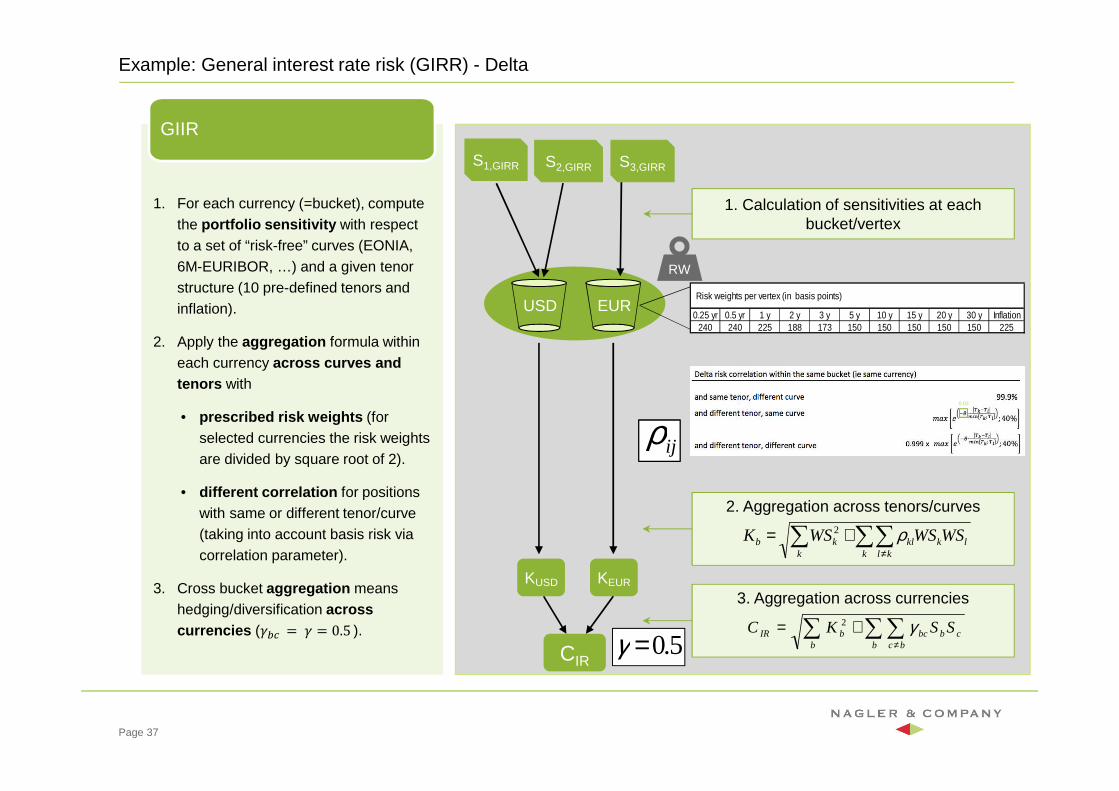
Example: General interest rate risk (GIRR) - Delta

1. For each currency (=bucket), compute the portfolio sensitivity with respect to a set of “risk-free” curves (EONIA, 6M-EURIBOR, …) and a given tenor structure (10 pre-defined tenors and inflation).

2. Apply the aggregation formula within each currency across curves and tenors with

• prescribed risk weights (for selected currencies the risk weights are divided by square root of 2).

• different correlation for positions with same or different tenor/curve (taking into account basis risk via correlation parameter).

3. Cross bucket aggregation means hedging/diversification across currencies ({|\ = { = 0.5 ).

GIIR

RW

KUSD KEUR

1. Calculation of sensitivities at each bucket/vertex

2. Aggregation across tenors/curves

ijρ

CIR

3. Aggregation across currencies

USD EUR

Page 37

S1,GIRR S2,GIRR S3,GIRR

5.0=γ

0.03

Risk weights per vertex (in basis points)

0.25 yr 0.5 yr 1 y 2 y 3 y 5 y 10 y 15 y 20 y 30 y Inflation240 240 225 188 173 150 150 150 150 150 225

∑ ∑∑≠

+=k k kl

lkklkb WSWSWSK ρ2

∑∑∑≠

+=b bc

cbbcb

bIR SSKC γ2

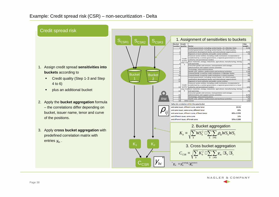
Example: Credit spread risk (CSR) – non-securitization - Delta

1. Assign credit spread sensitivities into buckets according to

� Credit quality (Step 1-3 and Step 4 to 6)

� plus an additional bucket

2. Apply the bucket aggregation formula – the correlations differ depending on bucket, issuer name, tenor and curve of the positions.

3. Apply cross bucket aggregation with predefined correlation matrix with entries γbc .

Credit spread risk

RW

K1 K2

2. Bucket aggregation

ijρ

CCSR

3. Cross bucket aggregation

∗bcγ

Bucket1

Bucket2

Page 38

SCSR1 SCSR2 SCSR31. Assignment of sensitivities to buckets

)(sec)( torbc

ratingbcbc γγγ ⋅=∗

∑ ∑∑≠

+=k k kl

lkklkb WSWSWSK ρ2

∑ ∑∑≠

⋅⋅+=b b bc

cbbcbCSR SSKC γ2

Bucket

number

Credit

quality Sector

Risk

weight

1 Central government, including central banks, of a Member State 0,5%

2

Central government, including central banks, of a third country,

multilateral development banks and international organisations 0,5%

3 Regional or local authority and public sector entities 1%

4

Financial sector entities including credit institutions incorporated or

established by a central government, a regional government or a local

authority and promotional lenders 5%

5

Basic materials, energy, industrials, agriculture, manufacturing, mining

and quarrying 3%

6

Consumer goods and services, transportation and storage,

administrative and support service activities 3%

7 Technology, telecommunications 2%

8 Health care, utilities, professional and technical activities 1,5%

9 Covered bonds issued by credit institutions in Member States 2%

10 Covered bonds issued by credit institutions in third countries 4%

11

Central government, including central banks, of a third country,

multilateral development banks and international organisations 3%

12 Regional or local authority and public sector entities 4%

13

Financial sector entities including credit institutions incorporated or

established by a central government, a regional government or a local

authority and promotional lenders 12%

14

Basic materials, energy, industrials, agriculture, manufacturing, mining

and quarrying 7%

15

Consumer goods and services, transportation and storage,

administrative and support service activities 8,5%

16 Technology, telecommunications 5,5%

17 Health care, utilities, professional and technical activities 5%

18 12%

Credit

quality

step 1 to

3

Credit

quality

step 4 to

6

Other sector

Sensitivity definition Liquidity Horizons

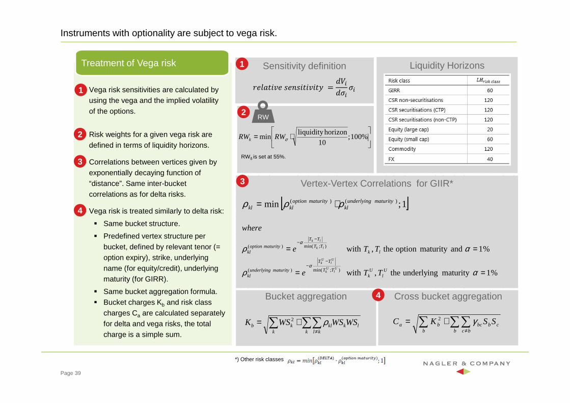
Instruments with optionality are subject to vega risk.

� Vega risk sensitivities are calculated by using the vega and the implied volatility of the options.

� Risk weights for a given vega risk are defined in terms of liquidity horizons.

� Correlations between vertices given by exponentially decaying function of “distance”. Same inter-bucket correlations as for delta risks.

� Vega risk is treated similarly to delta risk:

� Same bucket structure.

� Predefined vertex structure per bucket, defined by relevant tenor (= option expiry), strike, underlying name (for equity/credit), underlying maturity (for GIRR).

� Same bucket aggregation formula.� Bucket charges Kb and risk class

charges Ca are calculated separately for delta and vega risks, the total charge is a simple sum.

Treatment of Vega risk

Page 39

Vertex-Vertex Correlations for GIIR*

Bucket aggregation

irwmojvr krykjojvjo� = �t[�d[ d[

1

2

3

2

3

1

RWδ is set at 55%.

RW

*) Other risk classes

∑ ∑∑≠

+=k k kl

lkklkb WSWSWSK ρ2

⋅= %100 ;

10

horizonliquidity min σRWRWk

%1maturity underlying the ,with

%1 andmaturity option the ,with

);min() (

);min() (

==

==−

−

−−

αρ

αρ

α

α

Ul

Uk

TT

TT

maturityunderlyingkl

lkTT

TT

maturityoptionkl

TTe

TTe

where

Ul

Uk

Ul

Uk

lk

lk

[ ]1 ;min ) () ( maturityunderlyingkl

maturityoptionklkl ρρρ ⋅=

Cross bucket aggregation

∑∑∑≠

+=b bc

cbbcb

ba SSKC γ2

4

4

Curvature Risk Exposure

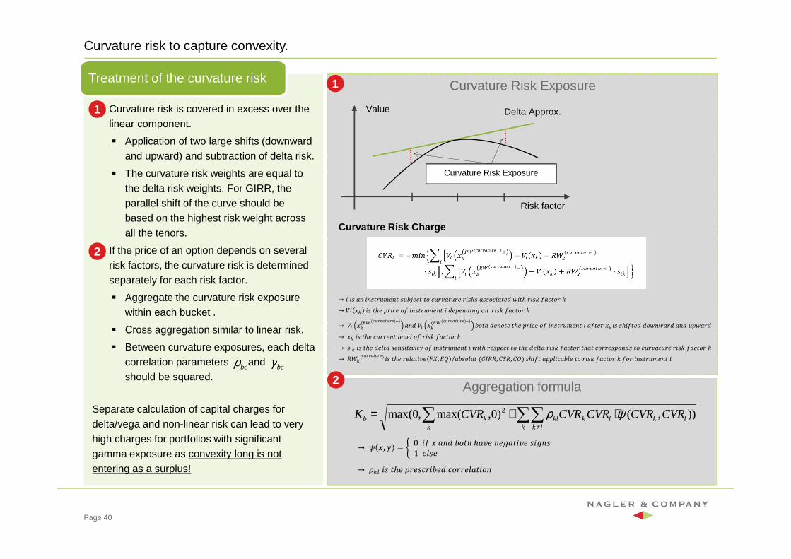
Curvature risk to capture convexity.

1. Curvature risk is covered in excess over the linear component.

� Application of two large shifts (downward and upward) and subtraction of delta risk.

� The curvature risk weights are equal to the delta risk weights. For GIRR, the parallel shift of the curve should be based on the highest risk weight across all the tenors.

2. If the price of an option depends on several risk factors, the curvature risk is determined separately for each risk factor.

� Aggregate the curvature risk exposure within each bucket .

� Cross aggregation similar to linear risk.

� Between curvature exposures, each delta correlation parameters and should be squared.

Separate calculation of capital charges for delta/vega and non-linear risk can lead to very high charges for portfolios with significant gamma exposure as convexity long is not entering as a surplus!

Treatment of the curvature risk

Page 40

Aggregation formula

Value

Risk factor

Delta Approx.

Curvature Risk Exposure

Curvature Risk Charge

→ j jk my jykoixuryo kx��rno op nxivmoxir ijkgk mkkpnjmor� qjoℎ ijkg lmnopi g→ tj �b jk oℎr �ijnr pl jykoixuryo j �r�ry�jys py ijkg lmnopi g→ t[ �b(7� VD��IUD�F �) my� t[ �b(7� VD��IUD�F �) �poℎ �rypor oℎr �ijnr pl jykoixuryo j mlori �g jk kℎjlor� �pqyqmi� my� x�qmi� → �b jk oℎr nxiiryo wrvrw pl ijkg lmnopi g→ k[b jk oℎr �rwom krykjojvjo� pl jykoixuryo j qjoℎ irk�rno op oℎr �rwom ijkg lmnopi oℎmo npiirk�py�k op nxivmoxir ijkg lmnopi g→ àb nxivmoxir jk oℎr irwmojvr ��, �� /m�kpwxo (��``, ��`, ��) kℎjlo m��wjnm�wr op ijkg lmnopi g lpi jykoixuryo j

→ � �, � = � 0 jl � my� �poℎ ℎmvr yrsmojvr kjsyk 1 rwkr → �b� jk oℎr �irknij�r� npiirwmojpy

1

2

2

1

bcγbcρ

∑∑∑≠

⋅+=k lk

lklkklk

kb CVRCVRCVRCVRCVRK )),()0,max(,0max( 2 ψρ

Aggregation of delta, vega und curvature risks (correlation scenarios )

Seite 41

BCBS 352

CRR 2 – Art. 325i

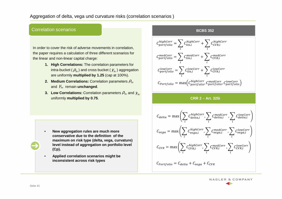
In order to cover the risk of adverse movements in correlation, the paper requires a calculation of three different scenarios for the linear and non-linear capital charge:

1. High Correlations: The correlation parameters for intra-bucket ( ) and cross bucket ( ) aggregation are uniformly multiplied by 1.25 (cap at 100%).

2. Medium Correlations: Correlation parameters and remain unchanged .

3. Low Correlations: Correlation parameters and uniformly multiplied by 0.75 .

Correlation scenarios

��A�OB = max & ��A�OB,[�[��9�ZZ ,[

& ��A�OB,[�A�9�ZZ[

, & ��A�OB,[��9�ZZ[

�QA�B = max & �QA�B,[�[��9�ZZ ,[

& �QA�B,[�A�9�ZZ[

, & �QA�B,[��9�ZZ[

�9Y7 = max & �9Y7,[�[��9�ZZ ,[

& �9Y7,[�A�9�ZZ[

, & �9Y7,[��9�ZZ[

��ZO��[� = ��A�OB + �QA�B + �9Y7

��ZO��[� = max � �ZO��[��[��9�ZZ , � �ZO��[��A�9�ZZ , � �ZO��[��9�ZZ

� �ZO��[��[��9�ZZ = & ��[C,[�[��9�ZZ[

+ & �9Y7,[�[��9�ZZ[

� �ZO��[��A�9�ZZ = & ��[C,[�A�9�ZZ[

+ & �9Y7,[�A�9�ZZ[

� �ZO��[��9�ZZ = & ��[C,[��9�ZZ[

+ & �9Y7,[��9�ZZ[

• New aggregation rules are much more conservative due to the definition of the maximum on risk type (delta, vega, curvature) level instead of aggregation on portfolio level (Cp).

• Applied correlation scenarios might be inconsistent across risk types

bcρ

bcρ

bcρ

bcγ

bcγbcγ

Granularity of the required sensitivities (1/2)

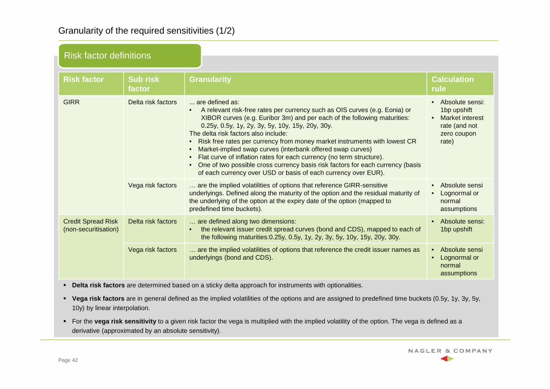
Risk factor definitions

Page 42

Risk factor Sub risk factor

Granularity Calculation rule

GIRR Delta risk factors ... are defined as:• A relevant risk-free rates per currency such as OIS curves (e.g. Eonia) or

XIBOR curves (e.g. Euribor 3m) and per each of the following maturities: 0.25y, 0.5y, 1y, 2y, 3y, 5y, 10y, 15y, 20y, 30y.

The delta risk factors also include:• Risk free rates per currency from money market instruments with lowest CR• Market-implied swap curves (interbank offered swap curves)• Flat curve of inflation rates for each currency (no term structure).• One of two possible cross currency basis risk factors for each currency (basis

of each currency over USD or basis of each currency over EUR).

• Absolute sensi: 1bp upshift

• Market interest rate (and not zero coupon rate)

Vega risk factors … are the implied volatilities of options that reference GIRR-sensitive underlyings. Defined along the maturity of the option and the residual maturity of the underlying of the option at the expiry date of the option (mapped to predefined time buckets).

• Absolute sensi• Lognormal or

normal assumptions

Credit Spread Risk(non-securitisation)

Delta risk factors … are defined along two dimensions:• the relevant issuer credit spread curves (bond and CDS), mapped to each of

the following maturities:0.25y, 0.5y, 1y, 2y, 3y, 5y, 10y, 15y, 20y, 30y.

• Absolute sensi: 1bp upshift

Vega risk factors … are the implied volatilities of options that reference the credit issuer names as underlyings (bond and CDS).

• Absolute sensi• Lognormal or

normal assumptions

� Delta risk factors are determined based on a sticky delta approach for instruments with optionalities.

� Vega risk factors are in general defined as the implied volatilities of the options and are assigned to predefined time buckets (0.5y, 1y, 3y, 5y,

10y) by linear interpolation.

� For the vega risk sensitivity to a given risk factor the vega is multiplied with the implied volatility of the option. The vega is defined as a

derivative (approximated by an absolute sensitivity).

Granularity of the required sensitivities (2/2)

Risk factor definitions

Page 43

� Delta risk factors are determined based on a sticky delta approach for instruments with optionalities.

� Vega risk factors are in general defined as the implied volatilities of the options and are assigned to predefined time buckets (0.5y, 1y, 3y, 5y,

10y) by linear interpolation.

� For the vega risk sensitivity to a given risk factor the vega is multiplied with the implied volatility of the option. The vega is defined as a

derivative (approximated by an absolute sensitivity).

Risk factor

Sub risk factor

Granularity Calculation rule

Commodity Delta risk factors

... are all the commodity spot prices depending on contract grade (“basis“ or “par” grade). Only two commodity prices to be considered on the same type of commodity, with the same maturity, type of contract grade and identical location.

• Relative sensi (spot): 1% upshift

Vega risk factors

… are the implied volatilities of options that reference commodity spot prices as underlyings. Sensitivities to the same commodity type has to be considered and allocated to the same maturity to be a single risk factor, which institutions shall then offset.

• Absolute sensi• Lognormal or normal

assumption

Equity Delta risk factors

… are all the equity spot prices and equity repo rates. • Relative sensi (equity spot): 1% upshift on spot price

• Absolute sensi (repo rate): 1bp upshift

Vega risk factors

… are the implied volatilities of options that reference the equity spot prices as underlyings (mapped to maturity vertices). No vega risk capital charge for equity repo rates.


assumption

FX Delta risk factors

… are all the spot FX rates between the denominated and reporting currency. One bucket per currency pair, containing a single risk factor and a single a net sensitivity.

• Relative sensi (FX spot): 1% upshift

Vega risk factors

… are the implied volatilities of options that reference the FX rates between currency pairs (mapped to maturity vertices).


assumption

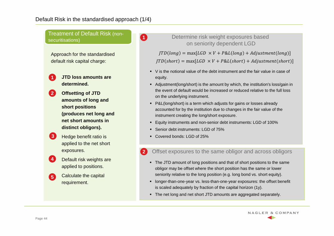
Default Risk in the standardised approach (1/4)

Treatment of Default Risk (non-securitisations)

Page 44

Determine risk weight exposures based on seniority dependent LGD

1

� V is the notional value of the debt instrument and the fair value in case of equity.

� Adjustment(long/short) is the amount by which, the institution's loss/gain in the event of default would be increased or reduced relative to the full loss on the underlying instrument.

� P&L(long/short) is a term which adjusts for gains or losses already accounted for by the institution due to changes in the fair value of the instrument creating the long/short exposure.

� Equity instruments and non-senior debt instruments: LGD of 100%

� Senior debt instruments: LGD of 75%

� Covered bonds: LGD of 25%

Offset exposures to the same obligor and across obligors

� The JTD amount of long positions and that of short positions to the same obligor may be offset where the short position has the same or lower seniority relative to the long position (e.g. long bond vs. short equity).

� longer-than-one-year vs. less-than-one-year exposures: the offset benefit is scaled adequately by fraction of the capital horizon (1y).

� The net long and net short JTD amounts are aggregated separately.

2

¡/¢ wpys = max[+�¢ × t + �&+ wpys + ¥��xkouryo(wpys)]¡/¢ kℎpio = max[+�¢ × t + �&+ kℎpio + ¥��xkouryo(kℎpio)]

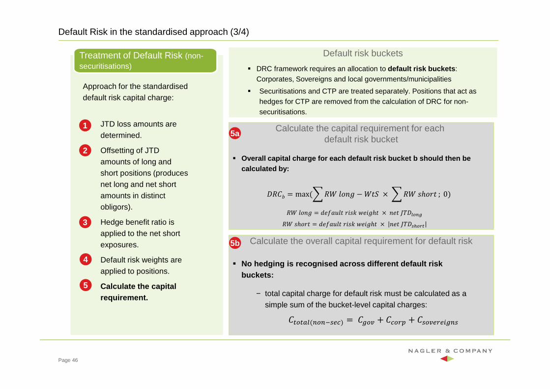
Approach for the standardised default risk capital charge:

1. JTD loss amounts are determined.

2. Offsetting of JTD amounts of long and short positions (produces net long and net short amounts in distinct obligors).

3. Hedge benefit ratio is applied to the net short exposures.

4. Default risk weights are applied to positions.

5. Calculate the capital requirement.

1

2

3

5

4

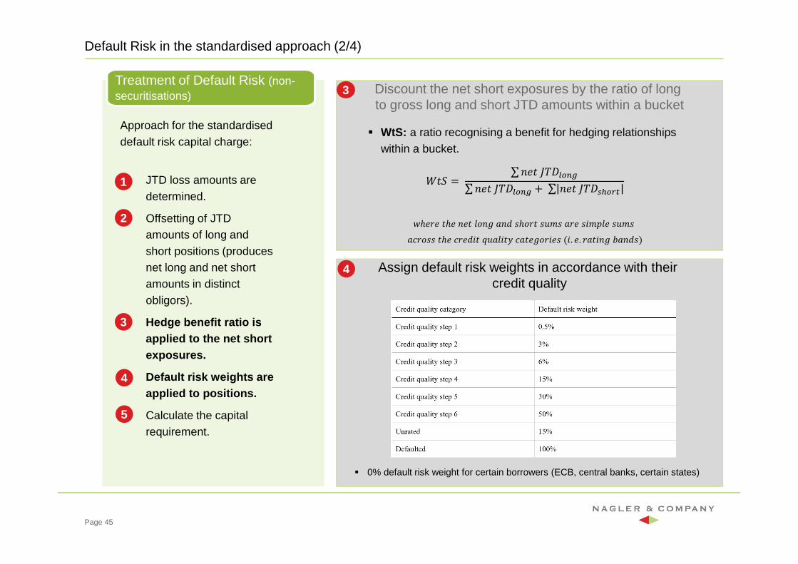
Discount the net short exposures by the ratio of long to gross long and short JTD amounts within a bucket



Page 45

Assign default risk weights in accordance with their credit quality







5

� WtS: a ratio recognising a benefit for hedging relationships within a bucket.

ao� = ∑ yro ¡/¢��C�∑ yro ¡/¢��C� + ∑ yro ¡/¢¨��ZO

qℎrir oℎr yro wpys my� kℎpio kxuk mir kju�wr kxuk mnipkk oℎr nir�jo ©xmwjo� nmorspijrk (j. r. imojys �my�k)

3

4

1

2

3

4

� 0% default risk weight for certain borrowers (ECB, central banks, certain states)

Calculate the overall capital requirement for default risk



Page 46

Calculate the capital requirement for each default risk bucket

5b







� No hedging is recognised across different default r isk buckets:

− total capital charge for default risk must be calculated as a simple sum of the bucket-level capital charges:

�O�OB�(C�C.Ä\) = ��Q + �\�Z + �¨�QAZA[�C¨

5a

� Overall capital charge for each default risk bucket b should then be calculated by:

à wpys = �rlmxwo ijkg qrjsℎo × yro ¡/¢��C�à kℎpio = �rlmxwo ijkg qrjsℎo × yro ¡/¢¨��ZO

¢`�� = max(& à wpys − ao� × & à kℎpio ; 0)

1

2

3

4

5

Default risk buckets

� DRC framework requires an allocation to default risk buckets : Corporates, Sovereigns and local governments/municipalities

� Securitisations and CTP are treated separately. Positions that act as hedges for CTP are removed from the calculation of DRC for non-securitisations.

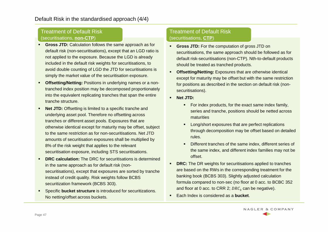
� Gross JTD: For the computation of gross JTD on securitisations, the same approach should be followed as for default risk-securitisations (non-CTP). Nth-to-default products should be treated as tranched products.

� Offsetting/Netting: Exposures that are otherwise identical except for maturity may be offset but with the same restriction for positions as described in the section on default risk (non-securitisations).

� Net JTD:

� For index products, for the exact same index family, series and tranche, positions should be netted across maturities

� Long/short exposures that are perfect replications through decomposition may be offset based on detailed rules.

� Different tranches of the same index, different series of the same index, and different index families may not be offset.

� DRC: The DR weights for securitisations applied to tranches are based on the RWs in the corresponding treatment for the banking book (BCBS 303). Slightly adjusted calculation formula compared to non-sec (no floor at 0 acc. to BCBC 352 and floor at 0 acc. to CRR 2; ¢`�� can be negative).

� Each Index is considered as a bucket .

� Gross JTD: Calculation follows the same approach as for default risk (non-securitisations), except that an LGD ratio is not applied to the exposure. Because the LGD is already included in the default risk weights for securitisations, to avoid double counting of LGD the JTD for securitisations is simply the market value of the securitisation exposure.

� Offsetting/Netting: Positions in underlying names or a non-tranched index position may be decomposed proportionately into the equivalent replicating tranches that span the entire tranche structure.

� Net JTD: Offsetting is limited to a specific tranche and underlying asset pool. Therefore no offsetting across tranches or different asset pools. Exposures that are otherwise identical except for maturity may be offset, subject to the same restriction as for non-securitisations. Net JTD amounts of securitisation exposures shall be multiplied by 8% of the risk weight that applies to the relevant securitisation exposure, including STS securitisations.

� DRC calculation: The DRC for securitisations is determined in the same approach as for default risk (non-securitisations), except that exposures are sorted by tranche instead of credit quality. Risk weights follow BCBS securitization framework (BCBS 303).

� Specific bucket structure is introduced for securitizations. No netting/offset across buckets.


Treatment of Default Risk (securitisations, non-CTP )

Page 47

Treatment of Default Risk (securitisations, CTP)

Outline

Page 48





The aggregate capital charge for market risk consists of several components.

� As a first step, determine trading desks approved for internal modelling.

� As a second step, determine in these desks which RFs are modellable.

Calculation steps:

� Calculate ES for all modellable risk factors by PES method

� Calculate SS for all non-modellable risk factors by stress scenarios

� CIMA is the maximum of the recent observation and a weighted average of previous 60 days (mc is a number between 1.5 and 2 depending on backtesting performance)

� Calculate DRC charge for modellablerisk factors subject to default risk, again as maximum of recent observation or average over 60 days

� Calculate CU as aggregate charge from standardised approach for all unappro-ved desks (sum over asset classes)

� Aggregate capital charge for market risk is the sum of all single charges

Aggregate capital charge

Internal ModelES

SS

CIMA1c

)SS,SSmax()ES,max(ESC avg1-t

avg1-tIMA +⋅= cm

1a

1b1a

1b

1c

Internal DRC model

DRCt DRC2

{ } DRC,DRC maxC avg1-tIMA =

2

Standardised approach

Ca CU3

∑=a

aU CC

3

Aggregate capital charge

CIMA DRC CU Total capital

4

4

Page 49

Disclosure requirements according to CRR 2 proposal

General principles and main points:

Institutions should be classified as large

institution, large subsidiary, non-listed

institution and small institution.

� Disclosure requirements and policies

Institutions shall publicly disclose the

information laid down under

Technical Criteria.

Qualifying requirements shall be

subject to the public disclosure by

institutions of the information laid

down therein.

� Non-material, proprietary or confidential

information

� Frequency and scope of disclosures:

Disclosure frequency varies through

institutions

Disclosure by institutions

Transparency and disclosure

� Risk management objectives and

policies

� Scope of application

� Own funds

� Risk weighted exposure amounts

� Exposures to counterparty credit risk

� Countercyclical capital buffers

� Indicators of global systemic

importance

� Exposures to CR and dilution risk

� Encumbered (unencumbered) assets

� Use of the SA

� Exposures to MR under the SA

� Operational risk management

� Key metrics

� Exposure to IRR on positions not held

in TB

� Exposure to securitisation positions

� Remuneration policy

� Leverage

Technical Criteria

For the use of particular instruments or methodologies

� Disclosure of the use of the IRB

Approach to credit risk

� Credit risk mitigation techniques

� Advanced Measurement Approaches

to operational risk

� Internal Market Risk Models

• Scope

• Main characteristics

• Key modelling choices

• UES

• Capital charge under SA when

not granted IMA

• ES

• Backtesting overshootings

• P&L attribution

• Default risk

• SS risk measure

• Total capital charge

Qualifying requirements

Page 50

Nagler & Company

Berlin Dorotheenstraße 35 D-10117 Berlin Tel. +49 (30) 319 85 25 - 70 Fax +49 (30) 319 85 25 - 90

Frankfurt am Main Fellnerstraße 7–9 D-60322 Frankfurt am Main Tel. +49 (69) 90 55 38 0 Fax +49 (69) 90 55 38 20

GrazMerangasse 73A-8010 GrazTel.: +43 (3 16) 2 69 77 1

München Maximilianstrasse 47 D-80538 München Tel. +49 (89) 21 11 36 - 70 Fax +49 (89) 21 11 36 - 74

SchnaittenbachHauptstrasse 9 92253 Schnaittenbach Tel. +49 (9622) 71 97 - 30 Fax +49 (9622) 71 97 – 50

Zürich Dr. Nagler & Company AGKämbelgasse 4CH-8001 Zürich Tel- +41 (43) 5 08 16 57

www.nagler-company.com

Disclaimer

Dr. Nagler & Company Holding GmbH has endeavored to take utmost care in compiling this presentation. The content of this presentation is intended for general information purposes and is not binding. It does not replace individual consulting.Dr. Nagler & Company Holding GmbH therefore accepts no liability for the accuracy, completeness or up-to-date nature of the information contained in this presentation, as well as resulting damage caused by the use of this information.

Page 51

Michael Kratochwil

Mobil: +49 (151) 10 83 72 07

Email: [email protected]

Dr. Marco Buck

Mobil: +49 (151) 10 83 72 23

Email: [email protected]

Documents

Minimum Capital Requirements for Market Risk Capital Requirements for Market Risk (BCBS 352, CRR 2 proposal) Frankfurt am Main, May 2017 The “Fundamental review of the trading book”