BIS CCA-004-2010

May 2010

Macroprudential regulation and systemic capital requirements

A paper prepared for the BIS CCA Conference on

“Systemic risk, bank behaviour and regulation over the business cycle”

Buenos Aires, 18–19 March 2010

Authors*: Celine Gauthier, Alfred Lehar and Moez Souissi

Affiliation: Bank of Canada, Haskayne School of Business/University of Calgary

Email: alfred.lehar@haskayne.ucalgary.ca

* This paper reflects the views of the authors and not necessarily those of the BIS or of central banks

participating in the meeting.

Macroprudential regulationand systemic capital requirements ∗

Celine Gauthier†

Bank of CanadaFinancial Stability Department

Alfred Lehar‡

University of CalgaryHaskayne School of Business

Moez Souissi§

Bank of CanadaFinancial Stability Department

Abstract

In the aftermath of the financial crisis, there is interest in reforming bank regulation suchthat capital requirements are more closely linked to a bank’s contribution to the overall riskof the financial system. In our paper we compare alternative mechanisms for allocatingthe overall risk of a banking system to its member banks. Overall risk is estimated usinga model that explicitly incorporates contagion externalities present in the financial system.We have access to a unique data set of the Canadian banking system, which includes indi-vidual banks’ risk exposures as well as detailed information on interbank linkages includingOTC derivatives. We find that systemic capital allocations can differ by as much as 50%from 2008Q2 capital levels and are not related in a simple way to bank size or individualbank default probability. Systemic capital allocation mechanisms reduce default proba-bilities of individual banks as well as the probability of a systemic crisis by about 25%.Our results suggest that financial stability can be enhanced substantially by implementinga systemic perspective on bank regulation.Keywords: Systemic Risk, Financial Stability, Bank regulation, Risk Management, Inter-bank MarketJEL-Classification Numbers: G21, C15, C81, E44

∗The views and findings of this paper are entirely those of the authors and do not necessarily represent theviews of the Bank of Canada. We thank Sbastien Blais, Ian Christensen, Prasanna Gai, Toni Gravelle, ScottHendry, Miroslav Misina, Jacques Prfontaine, Mark Zelmer, and especially Allan Crawford for helpful comments.†e-mail: CGauthier@bank-banque-canada.ca, Tel: 613) 782-8699‡Corresponding author, Haskayne School of Business, University of Calgary, 2500 University Drive NW, Cal-

gary, Alberta, Canada T2N 1N4. e-mail: alfred.lehar@haskayne.ucalgary.ca, Tel: (403) 220 4567.§e-mail: msouissi@bank-banque-canada.ca, Tel:(613) 782 8631

1 Introduction

Under our plan ... financial firms will be required to follow the example of millions

of families across the country that are saving more money as a precaution against

bad times. They will be required to keep more capital and liquid assets on hand

and, importantly, the biggest, most interconnected firms will be required to keep

even bigger cushions. (Geithner (2009))

The recent financial crisis has demonstrated the adverse effects of a large scale breakdown

of financial intermediation for the rest of the economy. While academics, international institu-

tions, and central bankers have argued for some time that bank regulation should be designed

from a systemic perspective (Borio (2002), Gauthier and St-Amant (2005)), bank regulation is

currently aimed at the level of the individual bank, without taking any externalities inherent to

the financial system into account. In the aftermath of the financial crisis, there is a growing

consensus to bring a macroprudential perspective into bank regulation. One proposal is to re-

quire financial institutions to internalize the externalities they impose on the system by adjusting

capital requirements so that they better reflect an individual bank’s contribution to the overall

risk of the financial system. We refer to these adjusted capital requirements as systemic capital

requirements.

In this paper, we compare five approaches to assigning systemic capital requirements to in-

dividual banks based on each bank’s contribution to systemic risk:component and incremental

value-at-risk from the risk management literature (Jorion (2007)), two allocation strategies us-

ing Shapley values,1 and the ∆CoVaR measure introduced by Adrian and Brunnermeier (2009).

Computing systemic capital requirements, however, is more complex than computing risk con-

tributions. Setting required capital equal to risk contributions based on current observed capital

levels is insufficient because total risk in the banking system will change once new capital re-

quirements are implemented. We therefore have to follow an iterative procedure to solve for a

fixed point for which capital allocations to each bank are consistent with the contributions of

each bank to the total risk of the banking system. To our knowledge, we are the first to do so.

Before the allocation process can begin, we measure systemic risk using a model of banking

losses under a macro stress scenario. We build upon the models developed by central banks

1Shapley values are commonly used in the literature on risk allocation. Denault (2001) reviews some of therisk allocation mechanisms used in this paper, including the Shapley value. See also Kalkbrener (2005).

2

which include spillover and contagion effects through network and asset fire sale externalities

(e.g. Aikman, Alessandri, Eklund, Gai, Kapadia, Martin, Mora, Sterne, and Willison (2009)).

We do not allow for any endogenous reactions by the government or central bank, since these

would reduce the impact of the externalities we precisely want to measure.

We generate a macro stress scenario which causes varying increases in probabilities of

defaults (PD) for different economic sectors affecting all banks’ loan portfolios. Following

Elsinger, Lehar, and Summer (2006a), we simulate loan losses for each bank using a portfolio

credit risk model. Using a variant of Cifuentes, Shin, and Ferrucci (2005) that differentiates

banks according to the riskiness of their assets, banks that fall short of regulatory capital re-

quirements start selling assets to a market with inelastic demand and the resulting drop in prices

forces other banks to sell assets as well. Banks that default either because of loan losses or de-

creasing asset valuations are not able to fully honor their interbank promises, potentially causing

the contagious default of other banks. These spillover effects make the correlation of banks’

asset values dependent of the health of the overall financial system. Clearing in the interbank

market is captured using a Eisenberg and Noe (2001) network model. We use a unique data

set of the six largest Canadian banks as a representation of the whole Canadian banking system

since they hold 90.3% of all banking assets. Our sample contains detailed information on the

composition of the loan book, including the largest loan exposures of individual banks. As in

previous studies (see Upper (2007) for a summary), our data covers exposures between banks

arising from traditional lending. We expand this set of exposures by also covering those arising

from another on-balance sheet item, cross-shareholdings, and from off-balance sheet instru-

ments such as exposures related to exchange traded and OTC derivatives. While derivatives are

often blamed for creating systemic risk, the lack of data in many countries (including the U.S.)

makes it hard to verify. Our expanded dataset enables us to better capture linkages among banks

and contagious bank defaults.

With the same amount of overall capital in the banking system, we find that systemic capital

requirements can reduce default risk of the individual bank as well as the risk of a systemic crisis

by about 25%. Systemic capital allocations differ from current observed capital levels by up to

50% for individual banks, and the reallocation of capital that the macroprudential rules suggest

are not related in a simple way to bank size, bank PD, or risk weighted assets. We also find

that ignoring our information on derivatives and cross shareholdings gives us a very different

picture of individual bank risk with potential important effects on systemic risk. This speaks to

the importance of getting better information about exposures between financial institutions.

3

In the literature we find two main approaches to measure and allocate systemic risk. One

stream uses stock market data to get information on banks’ correlation structure and potential

spillovers. Adrian and Brunnermeier (2009) propose the CoVaR measure, which they compute

for a panel of financial institutions and regress on bank characteristics. This literature is related

to existing studies of contagion in financial markets (see among others Forbes and Rigobon

(2002), Bae, Karolyi, and Stulz (2003)). Another stream of research builds on a network model

in conjunction with an interbank clearing algorithm introduced by Eisenberg and Noe (2001).

Elsinger, Lehar, and Summer (2006a) and Aikman, Alessandri, Eklund, Gai, Kapadia, Mar-

tin, Mora, Sterne, and Willison (2009) use a dataset of interbank linkages for the Austrian and

British banking system, respectively, and compute measures of systemic risk and systemic im-

portance for individual banks. Upper (2007) reviews that literature.

These two approaches can be interpreted in light of economic theories of financial amplifi-

cation mechanisms at work during crisis. For example, Allen and Gale (1994) seminal paper

shows how asset prices can be optimally determined by cash-in-the-market in crisis periods.

Allen and Gale (2000) propose a model of contagion through a network of interbank exposures.

Shin (2008) develops a theory of liquidity spillover across a network of financial institutions re-

sulting from expansions and contractions of balance sheets over the credit cycle. Krishnamurthy

(2009) reviews the literature on the mechanisms involving balance-sheet and asset prices, and

those involving investors’ Knightian uncertainty. Tarashev, Borio, and Tsatsaronis (2009) con-

duct a simulation study of a stylized banking system and find that the systemic importance of an

institution increases in its size as well as its exposure to common risk factors. They use Shapley

values to allocate risk measured by value-at-risk as well as expected loss.

We extend previous research in two ways: first we highlight that changing capital require-

ments change the risk and correlation structure in the banking system and that systemic capital

requirements have to be seen as a fixed point problem. Second we provide empirical evidence

that systemic capital requirements can reduce individual as well as systemic risk using actual

data for a whole banking system.

The paper is organized as follows. Section 2 describes the approaches to assign systemic

capital requirements, the model for assessing systemic risk is described in Section 3, and Section

4 details credit loss scenario generation and the data. We present the results in Section 5 and

give a conclusion in Section 6.

4

2 Systemic capital requirements

Setting systemic capital requirements raises two fundamental questions. First, what is the total

level of capital required in the banking system, which determines the overall magnitude of the

shock that a banking system can withstand? Second, how to break down the overall risk of

the banking system and set capital requirements equal to each banks’ contribution to systemic

risk? The first question is a policy decision balancing efficiency of financial intermediation with

overall stability of the system which we do not address in this paper. We focus on the second

question by comparing alternative mechanisms to reallocate capital among banks, for a given

level of total capital in the system.

Systemic capital requirements differ from risk contribution analysis as it is used in portfolio

or risk management. In a risk management or portfolio management setting we want to compute

risk contributions for a given portfolio with an exogenous level of overall risk. Using the same

approach to computee systemic capital requirements in a banking system would be incorrect

because both the overall risk and each bank’s contribution depend on the capital allocation.

As banks hold more capital they are less likely to default through direct losses and contagion.

Reallocating bank capital changes the overall risk of the banking system, particularly in the

presence of contagion.2

Estimating systemic capital requirements is therefore a fixed point problem. We have to

reallocate bank capital such that the risk contribution of each of the n banks to total risk equals

the allocated capital. Assume that there is a model, like the one in this paper, that estimates a

banking systems’ joint risk distribution Σ(C) for a given vector of bank capital endowments

C = (C1, ..., Cn). A risk sharing rule f(Σ) then allocates the overall risk Σ(C) to individual

banks. A consistent capital allocation C∗ must then satisfy

C∗ = f(Σ(C∗)). (1)

Because of the high degree of non-linearity, the fixed point in equation (1) can only be found

2Changing bank capital requirements might also change individual bank risk because of a long-term incentiveto change banks asset portfolios. We do not consider this channel in our analysis for several reasons: systemiccapital requirements can be continuously adjusted as banks’ long term asset portfolios change. We also believethat the direct effect that changes in capital have on bank solvency risk outweigh the indirect incentive effects onbanks’ optimal asset choice.

5

numerically.3 From the discussion above it also becomes clear that we cannot find systemic

capital requirements without a model Σ(C) of the banking system’s risk. Our model, which we

describe in detail in Section 3, is simulation based. For each of our m simulated scenarios we

record the profit or loss for each bank to get the joint loss distribution for all banks, i.e. we get

an n ×m matrix of losses, which we call L. We then allocate the risk of the whole system to

each individual bank using different risk allocation methodologies f(.).

We now look at several risk sharing methodologies proposed in the literature and compare

bank PDs and measures of systemic stability under their respective fixed point capital alloca-

tions.

2.1 Component value-at-risk (beta)

Following Jorion (2007) we compute the contribution of each bank to overall risk as the beta of

the losses of each bank with respect to the losses of a portfolio of all banks. Let li,s be the loss of

bank i in scenario s and lp,s =∑

i li,s, then βi = cov(li,lp)

σ2(lp). Furthermore let Ci be the preexisting

tier 1 capital of bank i. We reallocate the total capital in the banking system according to the

following risk sharing rule

Cβi = βi

n∑i=1

Ci. (2)

where Cβi is the reallocated capital of bank i. A nice property of this rule is that the sum of

the betas equals one, so a redistribution of total capital amongst the banks is straightforward.

2.2 Incremental value-at-risk

We first compute the value-at-risk (VaR) of the joint loss distribution of the whole banking

system, which we get by adding the individual losses across banks in each simulated scenario.

We chose a confidence level of 99.5% and run 1,000,000 scenarios. The portfolio VaR, VaRp,

is therefore the 5,000th largest loss of the aggregate losses lp. Next we compute the VaR of

the joint distribution of all banks except bank i, VaR−i, as the 5,000th largest value of the

3We find that it takes on average 20 iterations until the norm of the changes in capital requirements from oneiteration to the next is less that $500,000.

6

l−is =∑n

j=1,j 6=i lj,s. The incremental VaR for bank i,iVaRi, is then defined as

iVaRi = VaRp − VaR−i. (3)

The incremental VaR therefore can be interpreted as the increase in risk that is generated by

adding bank i to the system.4

While component VaR computes the marginal impact of an increase in a bank’s size, in-

cremental VaR captures the full difference in risk that one bank will bring to the system. The

disadvantage of the second risk decomposition is that the sum of the incremental VaRs does not

add up to the VaR of the banking system. In our analysis, however, we found that difference to

be small (below 5%) and thus scale iVaR capital requirements as follows:

C iVaRi =

iVaRi∑i iVari

∑i

Ci. (4)

2.3 Shapley values

In a recent paper, Tarashev, Borio, and Tsatsaronis (2009) propose to use Shapley values to allo-

cate capital requirements to individual banks. Shapley values can be seen as efficient outcomes

of multi player allocation problems in which each player holds resources that can be combined

with others to create value. The Shapley value then allocates a fair amount to each player based

on the average marginal value that the player’s resource contributes to the total.5 In this context,

one can argue that a certain level of capital has to be provided by all banks as a buffer for the

banking system and that Shapley values help to determine how much capital each bank should

provide according to its relative contribution to overall risk.

To compute Shapley values we have to define the characteristic function v(B) for a set

B ⊆ N of banks, which assigns a capital requirement to each possible combination of banks.6

4We calculate VaR−i by adding the losses from all banks except bank i. Another way would be to remove banki from the banking system and then compute the loss distribution of the reduced system. We decided against thelatter approach, because removing a bank would leave holes in the remaining banks’ balance sheets when claimson bank i do not equal liabilities to bank i as it is the case in our sample.

5While Shapley values were originally developed as a concept of cooperative game theory, they are also equi-librium outcomes of noncooperative multi-party bargaining problems (see e.g. Gul (1989)).

6A potential caveat of this methodology is that all characteristic function games assume that the value v(B),which a group of banksB can achieve, is independent of how the other banks that are not inB group together. Davidand Lehar (2009) analyze under what conditions banks find it optimal to merge to avoid bankruptcy costs using a

7

In our analysis we use two risk measures to define capital requirements: expected tail loss (EL)

and value-at-risk. To compute v(B) we add the profits and losses for all the banks in B across

scenarios to get the joint loss distribution for B, i.e. lB,s =∑

i∈B li,s. We assume a confidence

level of 99.5% and then assign to v(B) either the corresponding VaR, which is the 5,000th

largest loss of lB, or the expected tail loss, i.e. the arithmetic average of the 5,000 biggest losses.

Define furthermore v(∅) = 0, then the Shapley value for bank i, equal to its capital requirement,

can be computed as:

φi(v) =∑B⊆N

|B|!(|N | − |B| − 1)!

|N |!(v(B ∪ i)− v(B)) (5)

Because the sum of the Shapley values will in general not add up to the total capital that is

currently employed in the banking system, we scale the Shapley values similar to Equation (4):

CSVi =

φi∑i φi

∑i

Ci. (6)

One potential caveat of all systemic capital requirements is that capital allocations can be

negative, for example if a bank is negatively correlated with the other banks and therefore

reduces the risk of the system. This problem also applies to the Shapley value procedure.

Unless we assume monotonicity, i.e. v(S ∪ T ) ≥ v(S) + v(T ), the core of the game can be

empty and negative Shapley values can be obtained. For our sample this problem did not occur

since bank correlations were sufficiently high.

2.4 ∆CoVaR

Following Adrian and Brunnermeier (2009) we define CoVaR as the value-at-risk of an insti-

tution conditional of the fact that the whole banking system has realized a loss corresponding

to its VaR. However, since we have to compute the joint loss distribution by simulation, we

observe cases for which aggregate banking system losses exactly equal the VaR with measure

zero. We therefore define CoVaR as

bargaining game in partition form, which defines the value of a coalition conditional on the coalition structure ofthe remaining banks. They find that under certain conditions bargaining can break down and inefficient liquidationsoccur.

8

Pr (li < CoVaRi | lp ∈ [VaRp(1− ε),VaRp(1 + ε)]) = 0.5% (7)

Where we set ε = 0.1.7 We then calculate

∆CoVaRi = CoVaRi − VaRi (8)

To get the overall capital requirements we scale the results with total capital

C∆CoVaRi =

∆CoVaRi∑i ∆CoVaRi

∑i

Ci. (9)

2.5 Benchmarks

One benchmark that we use against systemic capital requirements is banks’ current capital lev-

els. These might differ from minimum capital requirements as banks want to hold reserves

against unexpected losses from risks that are not included in current regulation. Capital levels

might also differ due to lumpiness in capital issuance. Most banks have issued new capital be-

fore our sample period and individual banks could not have found adequate investment projects

for all the funds that they have raised and thus show excessive capital levels. To address the

latter problem, we create a second benchmark, for which we redistribute the existing capital

such that each bank has the same regulatory capital ratio, which is defined as tier 1 capital over

risk weighted assets (RWA).8 We refer to this benchmark as the ”Basel equal” approach for the

rest of the paper:

CBasel equali =

RWAi∑i RWAi

∑i

Ci. (10)

We now turn to a description of the model used to generate the system loss distribution.

7We found that the capital requirements and the overall results are not significatly different for ε = 0.15 orε = 0.05.

8Under current Basel capital requirements, banks have to assign a risk weight to each asset that ranges fromzero for government backed assets to one for commercial loans. The RWA are the sum of asset values multipliesby their respective risk weight. The Basel accord requires at least 4% tier 1 capital, but countries are free to sethigher limits. Canada requires 7%.

9

3 A Model of the Banking System

We build upon the models developed in the recent literature on systemic risk in the financial

system. We first use a credit risk model to generate loan losses under a severe macroeconomic

recession (details are provided in Section 4). Following Aikman, Alessandri, Eklund, Gai,

Kapadia, Martin, Mora, Sterne, and Willison (2009), we then integrate a network model of

extended exposures between banks, and an endogenous asset fire sales (AFS) mechanism.9

To model the network of interbank obligations we extend the model of Eisenberg and Noe

(2001) to include bankruptcy costs and uncertainty as done by Elsinger, Lehar, and Summer

(2006a). Consider a set N = {1, ..., N} of banks. Each bank i ∈ N has a claim on specific

assets Ai outside of the banking system, which we can interpret as the bank’s portfolio of non-

bank loans and securities. Each bank is partially funded by issuing senior debt or deposits Lito outside investors. Bank i’s obligations against other banks j ∈ N are characterized by the

nominal liabilities xij .

The total value of a bank is the value of its assets minus the outside liabilities Ai − Li plus

the value of all net payments to and from counterparties in the banking system. If the total

value of a given bank becomes negative, the bank is insolvent. In this case we assume that its

assets are reduced by a proportional bankruptcy cost Φ. After outside debtholders are paid off,

any remaining value is distributed proportionally to creditor banks. We denote by d ∈ RN+ the

vector of total obligations of banks toward the rest of the system, i.e. di =∑

j∈N xij. We define

a new matrix Π ∈ [0, 1]N×N which is derived by normalizing xij by total obligations.

πij =

{xijdi

if di > 0

0 otherwise(11)

When an institution is unable to meet its obligations, it may be forced to sell assets at prices

well below their fair value to achieve a quick sale. We integrate the impact of such AFS of a

distressed institution on both its own mark-to-market balance sheet and those of other institu-

tions holding the same class of assets. For this purpose, we extend the work done by Cifuentes,

9No government or central bank interventions to limit fire sales of assets are allowed in the model. By doing so,we better measure the externalities imposed by riskier banks on others. However, banks likely default much morefrequently in our model than they would in practice. Different international working groups are currently studyingways to limit the occurrence of AFS in time of stress. Propositions include changes in margining practices, the useof central clearing platforms, and higher minimum capital requirements.

10

Shin, and Ferrucci (2005), in which banks were assumed equally risky, by differentiating banks

according to the riskiness of their assets. We assume that the equilibrium market price of the

illiquid assets of a bank is a decreasing function of their riskiness.

For each bank, the stock of outside assets, Ai, is divided into liquid and illiquid assets. Bank

i’s stock of liquid assets is given by ci and includes government’s securities and government

insured mortgages.10 Exposures between banks are also assumed liquid for simplicity. The

remainder of the bank’s assets, ei, are considered illiquid. The price of the illiquid asset of bank

i, pi, is determined in equilibrium, and the liquid asset has a constant price of 1. Thus the net

worth of bank i assuming all interbank claims get paid in full is

piei + ci +N∑j=1

πjidj − di − Li (12)

We model capital requirements in the spirit of the Basel II capital accord. Since all liquid

assets are backed by the government, they carry a zero risk-weight. Illiquid assets of bank i are

assumed to attract a risk-weight equal to the average risk-weight of the bank’s balance-sheet,

wi, and the average risk-weight of the banking sector assets is w.11 For the mark-to-market

value of the banks’ illiquid assets to reflect their riskiness, we assume that pi is a linear function

of the equilibrium average price p, and the deviation of the bank risk-weight from the banking

sector mean is

pi = min(1, p+ (w − wi)κ) (13)

where κ > 0 to ensure that assets sold by a riskier bank have lower mark-to-market value.12

We describe a banking system as a tuple (Π, E, C, L, d, P ) for which we define a clearing

payment vector X∗. The clearing payment vector has to respect limited liability of banks and

proportional sharing in case of default. It denotes the total payments made by the banks under

10We include insured mortgages because they also carry a zero risk-weight under Basel II capital requirementsand, as will be explained further below, selling zero risk-weight assets does not improve regulatory capital require-ments.

11A more realistic exercise would classify the bank’s assets in different risk class but this would increase con-siderably the complexity of the model.

12This simple functional form is chosen for illustrative purpose. Before our model could realistically be used toimpose new regulatory requirements on banks, a sensitivity analysis of other functional forms would be necessary.This is left for future work.

11

the clearing mechanism. Each component of X∗ is defined by

x∗i = min

[di,max

((piei + ci)

(1− Φ1[piei+ci+

∑jx∗jπji−Li<di]

)+∑j

x∗jπji − Li, 0

)](14)

To find a clearing payment vector, we employ a variant of the fictitious default algorithm devel-

oped by Eisenberg and Noe (2001).

Banks must satisfy a minimum capital ratio which stipulates that the ratio of the bank’s Tier

1 capital to the mark-to-market value of its assets must be above some prespecified minimum

r∗13 When a bank violates this constraint, we assume that it has to sell assets to reduce the size

of its balance-sheet.14 We denote by si the units of illiquid assets sold by bank i.15 Whereas

Cifuentes, Shin, and Ferrucci (2005) used a simple (non risk-weighted) leverage ratio, our con-

straint is closer in spirit to the Basel II accord in which banks have to hold capital commensurate

with the risk on their balance sheet. 16 Our minimum capital requirement is therefore given by

piei + ci +∑j

xiπji − xi − L

wipi(ei − si)≥ r∗. (15)

The numerator is the equity value of the bank where the interbank claims and liabilities are

calculated in terms of the realized payments. The denominator is the marked-to-market risk-

weighted value of the bank’s assets after the sale of si units of the illiquid assets. The underlying

assumption is that assets are sold for cash and cash does not have a capital requirement. Thus

if the bank sells si units of the illiquid assets, the value of the numerator is unchanged since

this involves only a transformation of assets into cash, while the denominator is decreased since

cash has zero risk-weight. Thus, by selling some illiquid assets, the bank can reduce the size of

its balance-sheet and increase the capital asset ratio.17

13In the numerical exercise, the required minimum is set at 7%, as imposed by the Canadian regulator.14We do not consider the possibility of raising fresh capital nor the need to sell assets because of a loss of

funding. The consequences of the latter would be similar to those described here, assuming the assets would haveto be sold at a discount.

15Selling liquid assets does not help to reduce the size of the balance-sheet because of their zero-risk weight.Note however, that holding more liquid assets reduces the size of the balance-sheet ex-ante.

16In addition to the distinction between liquid and illiquid assets done in Cifuentes, Shin, and Ferrucci (2005),we differentiate banks according to the riskiness of their illiquid assets. Without doing so, riskier banks wouldunrealistically find it easier to reduce the size of their balance-sheets.

17A decrease in price should be seen as the average price decrease of all the illiquid assets on the balance-sheet,some assets’ price potentially being unaffected while others suffering from huge mark-to-market losses.

12

We make the assumption that banks cannot short-sell assets. Thus si ∈ [0, ei]. An equi-

librium is the triple (X∗, S∗, P ∗) consisting of a vector of payments, vector of sales of illiquid

assets , and vector of prices p of the illiquid assets such that:

• For all banks i ∈ N , x∗i is determined according to equation (14).

• For all banks i, s∗i is the smallest sale that ensures that the capital adequacy condition is

satisfied. If there is no value of si ∈ [0, ei] for which the capital condition is satisfied then

s∗i = ei.

• There is a downward sloping demand curve d−1(.) such that p∗ = d−1(∑i

s∗i ).

The first condition reiterates the limited liability of equity holders, and the priority of debt

holders over interbank liabilities.18 The second condition says that either the bank is liquidated

altogether, or its sales of illiquid assets reduces its assets sufficiently to comply with the capital

adequacy ratio. Finally, the third condition stipulates that the price of the illiquid assets is

determined by the intersection of a downward-sloping demand curve and the aggregate supply

curve.

The inverse demand curve for the illiquid asset is assumed to be

p = e−α(

∑isi)

(16)

where is α a positive constant.

By rearranging the capital condition in Equation (15), we can write the asset fire sale si as a

function of pi, where si = 0 if capital is already above the minimum required,

si = min

ei,max

0,

(1− r∗wi)piei + ci +∑j

xiπji − L− xi

−r∗wipi

(17)

Since each si(p) is decreasing in p, the aggregate sale function is decreasing in p. The lower

the price, the lower the mark-to-market value of banks’ assets, and the bigger the need to sell

18In reality, the legal situation might be more complicated and the seniority structure might differ from thesimple procedure we employ here.

13

assets to bring capital ratios in line with the required regulatory minimum. The price adjustment

process is illustrated in Cifuentes, Shin, and Ferrucci (2005).19

An equilibrium price of the illiquid asset is a price p∗ such that aggregate supply is equal to

demand

p∗ = d−1

(∑i

si (p∗ + (w − wi)κ)

)(18)

From the solution of the clearing problem, we can gain additional economically important

information with respect to systemic stability. A bank is in default whenever it cannot meet its

interbank obligations, (x∗i < di). We refer to the default of bank i as fundamental if bank i is

not able to honour its promises under the assumptions that all other banks honor their promises

and that prices are not affected by AFS (p = 1)

ei + ci +N∑j=1

πjidj − Li < di (19)

We define a bank to default because of AFS, whenever the bank is not in fundamental default

but cannot honour its interbank obligations at the equilibrium price of the illiquid assets, even

when all other banks meet their interbank obligations. An AFS default occurs when

ei + ci +N∑j=1

πjidj − Li > di and

p∗i ei + ci +N∑j=1

πjidj − Li < di (20)

A contagious default occurs, when bank i defaults only because other banks are not able to

19The demand curve (parameter α) and the asset price function (parameter κ) need to be calibrated such that anequilibrium price exists for all potential positive levels of aggregate supply. Special care must be taken to makesure that all individual asset prices are always between an exogenously fixed downward limit above zero,pmin, and1, the price when there is zero aggregate asset supply.

14

keep their promises, i.e.,

p∗i ei + ci +N∑j=1

πjidj − Li > di but

p∗i ei + ci +N∑j=1

πjix∗j − Li < di (21)

To use the model for risk analysis, we model shocks to banks’ asset values by introducing a

distribution of banks’ credit losses as described in Section 4. As there is no closed form solution

for the distribution of the clearing vector X∗, we have to resort to a simulation approach where

each draw from the credit loss distributions, which we refer to as a scenario, maps into new asset

values for each bank. We solve the clearing problem for each scenario numerically. Thus from

an ex-ante perspective we can assess expected default frequencies, and decompose insolvencies

across scenarios into fundamental, AFS, and contagious defaults.

Our network model is able to capture two properties that we believe are important in mod-

eling systemic risk: spillover effects and feedback loops. When a bank gets in distress it sells

assets or defaults on its interbank claims, causing externalities for other banks. An increase in a

bank’s PD will therefore make asset fire sales and default in the inter-bank market more likely,

and therefore increase the PDs of the other banks in the system. This spillover effect makes

the correlation of bank asset values dependent of the health of the overall system. When all

banks are well capitalized, asset fire sales and interbank defaults are unlikely and correlation of

banks asset portfolios is driven by the correlation in the outside assets, i.e. the loan portfolios,

alone. In an asset fire sale or contagion scenario, all asset values fall, exhibiting a correlation

close to one. As the capitalization of the whole banking system decreases, the probability of

realizing the asset fire sale or contagion scenario increases and thus the ex-ante asset and default

correlation.

The feedback effect is driven by the asset fire sale externalities and is described in detail

in Cifuentes, Shin, and Ferrucci (2005). When a bank start selling assets, prices drop, which

causes other banks to violate their capital requirements and forces them to sell assets as well,

causing all banks’ asset values to drop even further. This feedback effect accelerates bank

defaults as bank capitalization decreases.

To illustrate these two effects we compare our model to a Merton model. Figure 1 shows the

15

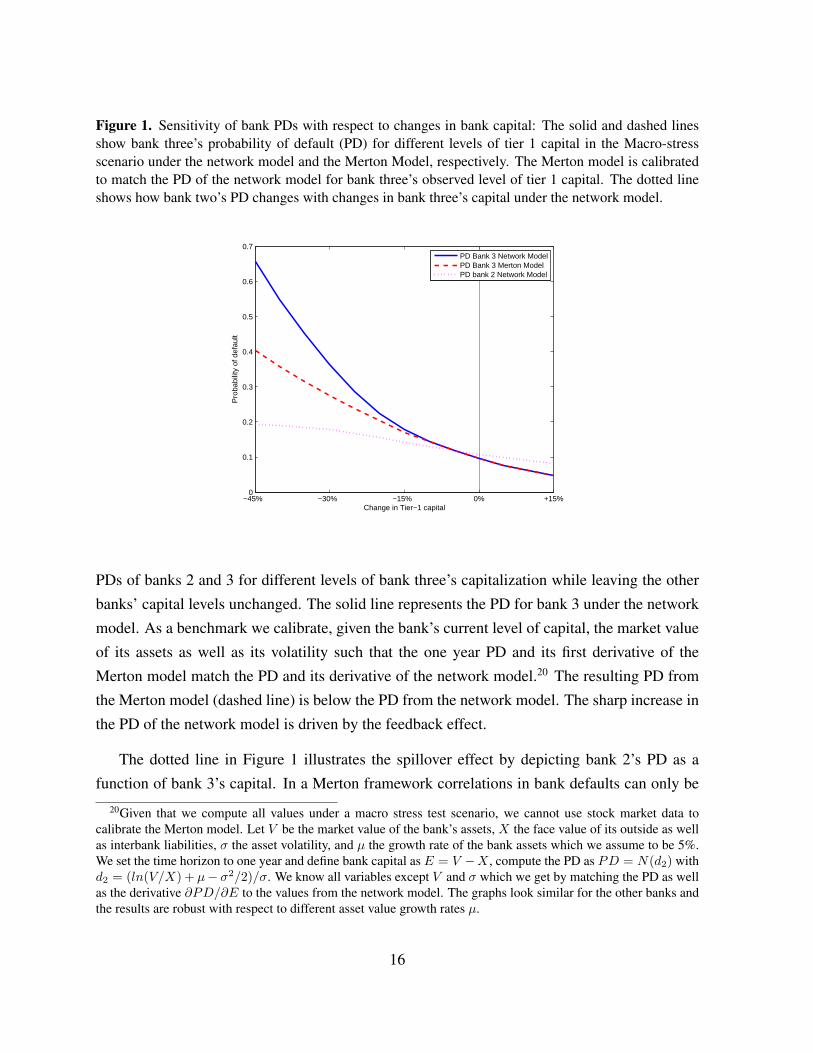
Figure 1. Sensitivity of bank PDs with respect to changes in bank capital: The solid and dashed linesshow bank three’s probability of default (PD) for different levels of tier 1 capital in the Macro-stressscenario under the network model and the Merton Model, respectively. The Merton model is calibratedto match the PD of the network model for bank three’s observed level of tier 1 capital. The dotted lineshows how bank two’s PD changes with changes in bank three’s capital under the network model.

−45% −30% −15% 0% +15%0

0.1

0.2

0.3

0.4

0.5

0.6

0.7

Change in Tier−1 capital

Pro

babi

lity

of d

efau

lt

PD Bank 3 Network ModelPD Bank 3 Merton ModelPD bank 2 Network Model

PDs of banks 2 and 3 for different levels of bank three’s capitalization while leaving the other

banks’ capital levels unchanged. The solid line represents the PD for bank 3 under the network

model. As a benchmark we calibrate, given the bank’s current level of capital, the market value

of its assets as well as its volatility such that the one year PD and its first derivative of the

Merton model match the PD and its derivative of the network model.20 The resulting PD from

the Merton model (dashed line) is below the PD from the network model. The sharp increase in

the PD of the network model is driven by the feedback effect.

The dotted line in Figure 1 illustrates the spillover effect by depicting bank 2’s PD as a

function of bank 3’s capital. In a Merton framework correlations in bank defaults can only be

20Given that we compute all values under a macro stress test scenario, we cannot use stock market data tocalibrate the Merton model. Let V be the market value of the bank’s assets, X the face value of its outside as wellas interbank liabilities, σ the asset volatility, and µ the growth rate of the bank assets which we assume to be 5%.We set the time horizon to one year and define bank capital as E = V −X , compute the PD as PD = N(d2) withd2 = (ln(V/X) + µ− σ2/2)/σ. We know all variables except V and σ which we get by matching the PD as wellas the derivative ∂PD/∂E to the values from the network model. The graphs look similar for the other banks andthe results are robust with respect to different asset value growth rates µ.

16

driven by asset correlations but changing one bank’s capitalization has no effect on other banks’

PDs. Asset fire sales and contagion externalities cause an increase in bank 2’s PD as bank 3

reduces its capital.

4 Data and credit loss distributions

4.1 Simulation of credit losses

For the modeling of credit losses, we combine simulation results of two models: a Bank of

Canada internal model, and an extended CreditRisk+ model.

The first model generates sectoral default rates that capture systematic factors affecting all

banks’ loans simultaneously. It relates the default rates of bank loans in different sectors to the

overall performance of the economy as captured by a selected set of macroeconomic variables.

The specification adopted for the model allows for non-linearities. Historical proxies for sec-

toral default rates were constructed based on sectoral bankruptcy rates.21 The included macroe-

conomic variables are GDP growth, unemployment rate, interest rate (medium-term business

loan rate), and the credit/GDP ratio. We simulate sectoral distributions of 10,000 default rates

for 2009Q2 under a severe recession macro scenario.22 The sectoral distributions of default

rates are centered on fitted values from sectoral regressions, and are generated using the corre-

lation structure of historical default rates.23 Descriptive statistics of these distributions as well

as historic peaks over the 1988-2006 period are presented in Table 1. Consistent with the sever-

ity of the macro scenario, mean default rates are much higher than historic peaks. Default rates

in the tail of the distributions are still higher.24

21The sectoral classification used in constructing the default rates is the one used by banks in reporting theirbalance sheet loan exposures. The seven sectors included were accommodation, agriculture, construction, man-ufacturing, retail, wholesale, and mortgages in the household sector. For more details on the construction ofhistorical default rates, see Misina and Tessier (2007).

22We use the macroeconomic scenario that was designed for the macro stress-testing exercise conducted as apart of Canada’s Financial Sector Assessment Program (FSAP) update in 2007. With a recession that is aboutone-third larger than experienced in the early 1990s, the stress-test scenario is plausible but extreme. See Lalonde,Misina, Muir, St-Amant, and Tessier (2008) for a detailed description of the scenario.

23More specifically, for each sector, the mean of the distribution is the expected default rate under the scenario,while the dispersion is obtained by adding random draws from the variance/covariance matrix of the historicalsectoral default rates. See Misina, Tessier, and Dey (2006) for more details on the simulation of default rates.

24A key component in modeling credit losses is banks’ sectoral Exposure-at default (EAD). Since the sectoral

17

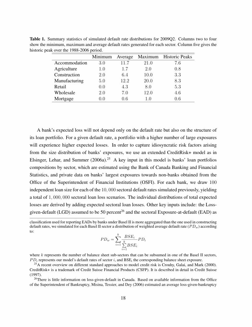
Table 1. Summary statistics of simulated default rate distributions for 2009Q2. Columns two to fourshow the minimum, maximum and average default rates generated for each sector. Column five gives thehistoric peak over the 1988-2006 period.

Minimum Average Maximum Historic PeaksAccommodation 3.0 11.7 21.0 7.6Agriculture 1.0 1.7 2.0 0.8Construction 2.0 6.4 10.0 3.3Manufacturing 5.0 12.2 20.0 8.3Retail 0.0 4.3 8.0 5.3Wholesale 2.0 7.0 12.0 4.6Mortgage 0.0 0.6 1.0 0.6

A bank’s expected loss will not depend only on the default rate but also on the structure of

its loan portfolio. For a given default rate, a portfolio with a higher number of large exposures

will experience higher expected losses. In order to capture idiosyncratic risk factors arising

from the size distribution of banks’ exposures, we use an extended CreditRisk+ model as in

Elsinger, Lehar, and Summer (2006a).25 A key input in this model is banks’ loan portfolios

compositions by sector, which are estimated using the Bank of Canada Banking and Financial

Statistics, and private data on banks’ largest exposures towards non-banks obtained from the

Office of the Superintendent of Financial Institutions (OSFI). For each bank, we draw 100

independent loan size for each of the 10, 000 sectoral default rates simulated previously, yielding

a total of 1, 000, 000 sectoral loan loss scenarios. The individual distributions of total expected

losses are derived by adding expected sectoral loan losses. Other key inputs include: the Loss-

given-default (LGD) assumed to be 50 percent26 and the sectoral Exposure-at-default (EAD) as

classification used for reporting EADs by banks under Basel II is more aggregated than the one used in constructingdefault rates, we simulated for each Basel II sector a distribution of weighted average default rate (PDw) accordingto:

PDw =k∑

i=1

BSEi

k∑i=1

BSEi

PDi

where k represents the number of balance sheet sub-sectors that can be subsumed in one of the Basel II sectors,PDi represents our model’s default rates of sector i, and BSEi the corresponding balance sheet exposure.

25A recent overview on different standard approaches to model credit risk is Crouhy, Galai, and Mark (2000).CreditRisk+ is a trademark of Credit Suisse Financial Products (CSFP). It is described in detail in Credit Suisse(1997).

26There is little information on loss-given-default in Canada. Based on available information from the Officeof the Superintendent of Bankruptcy, Misina, Tessier, and Dey (2006) estimated an average loss-given-bankruptcy

18

reported by banks.27

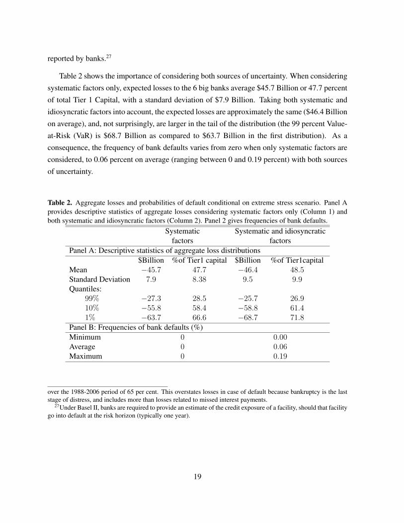
Table 2 shows the importance of considering both sources of uncertainty. When considering

systematic factors only, expected losses to the 6 big banks average $45.7 Billion or 47.7 percent

of total Tier 1 Capital, with a standard deviation of $7.9 Billion. Taking both systematic and

idiosyncratic factors into account, the expected losses are approximately the same ($46.4 Billion

on average), and, not surprisingly, are larger in the tail of the distribution (the 99 percent Value-

at-Risk (VaR) is $68.7 Billion as compared to $63.7 Billion in the first distribution). As a

consequence, the frequency of bank defaults varies from zero when only systematic factors are

considered, to 0.06 percent on average (ranging between 0 and 0.19 percent) with both sources

of uncertainty.

Table 2. Aggregate losses and probabilities of default conditional on extreme stress scenario. Panel Aprovides descriptive statistics of aggregate losses considering systematic factors only (Column 1) andboth systematic and idiosyncratic factors (Column 2). Panel 2 gives frequencies of bank defaults.

Systematic Systematic and idiosyncraticfactors factors

Panel A: Descriptive statistics of aggregate loss distributions$Billion %of Tier1 capital $Billion %of Tier1capital

Mean −45.7 47.7 −46.4 48.5Standard Deviation 7.9 8.38 9.5 9.9Quantiles:

99% −27.3 28.5 −25.7 26.910% −55.8 58.4 −58.8 61.41% −63.7 66.6 −68.7 71.8

Panel B: Frequencies of bank defaults (%)Minimum 0 0.00Average 0 0.06Maximum 0 0.19

over the 1988-2006 period of 65 per cent. This overstates losses in case of default because bankruptcy is the laststage of distress, and includes more than losses related to missed interest payments.

27Under Basel II, banks are required to provide an estimate of the credit exposure of a facility, should that facilitygo into default at the risk horizon (typically one year).

19

4.2 Data on exposures between major Canadian banks

As in previous studies of systemic risk in foreign banking systems (see among others Sheldon

and Maurer (1998), Wells (2002) and Upper and Worms (2004)), our data cover exposures

between banks that arise from traditional lending (unsecured loans and deposits). We improve

on previous literature by expanding this set of exposures. We also cover another on-balance

sheet item, cross-shareholdings, and off-balance sheet instruments such as exchange traded and

OTC derivatives. While derivatives are often blamed for creating systemic risk, the lack of data

in many countries (including the U.S.) makes it hard to verify. Our expanded dataset enables

us to better capture linkages among banks and contagious bank defaults.28 Of course, other

types of exposures between banks exist - most notably those coming from intraday payment

and settlement, from bank holdings of preferred banks’ shares (and other forms of capital),

and from holdings of debt instruments issued by banks like debentures and subordinated debt.

Owing to data limitations, however, the latter are not considered in this work.

Data on the exposures are collected on a consolidated basis and come from different sources

as described below. Available data are collected for May 2008 with the exception of exposures

related to derivatives which are recorded as of April 2008. We present descriptive statistics in

Table 3.29

Data on deposits and unsecured loans come from the banks’ monthly balance-sheet reports

to OSFI. These monthly reports reflect the aggregate asset and liability exposures of a bank for

deposits, and only aggregate asset exposures for unsecured loans. Data on exposures related to

derivatives come from a survey initiated by OSFI at the end of 2007. In that survey, banks are

asked to report their 100 largest mark-to-market counterparty exposures that were larger than

$25 million. These exposures were related to both OTC and exchange traded derivatives. They

are reported after netting and before collateral and guarantees.30

The reported data are used to construct a matrix of Big 6 banks’ bilateral exposures. Data

28Zero-risk exposures, mainly repo style transactions, were excluded despite their large size. They accountedfor more than 80 per cent of total exposures between the Big Six Canadian banks in 2008Q2. These exposuresmay represent a contagion channel in time of liquidity crisis, but this is left for future work.

29As it is standard in the network literature, we assume that there are two dates: the observation date and theclearing date when all interbank claims are settled. In this paper, we set 2009Q2 as the clearing date since ourdefault rates are simulated for a one-year horizon.

30The derivatives exposures reported may be biased upward, since they were reported before collateral andguarantees. In particular, anecdotal evidence suggests that the major Canadian banks often rely on high-qualitycollateral to mitigate their exposures to OTC derivatives.

20

on cross-shareholdings exposures were collected from Bank of Canada’s quarterly securities

returns.31

The aggregate size of interbank exposures was approximately $21.6 billion for the Six ma-

jor Canadian banks. As summarized in Table 3, total exposures between banks accounted for

around 25 per cent of bank capital on average. The available data suggest that exposures re-

lated to traditional lending (deposits and unsecured loans) were the largest ones compared with

mark-to-market derivatives and cross-shareholdings exposures. Indeed, in May 2008, exposures

related to traditional lending represented around $12.7 billion on aggregate, and 16.3 percent of

banks’ Tier 1 capital on average. Together, mark-to-market derivatives and cross-shareholdings

represented 10 per cent of banks’ Tier 1 capital on average.

A complete description of linkages between Canadian banks requires a complete matrix

of the bilateral exposures. Such a complete matrix was available only for exposures related

to derivatives. Unavailable bilateral exposures were estimated under the assumption that banks

spread their lending and borrowing as widely as possible across all other banks using an entropy

maximization algorithm (see e.g. Blien and Graef (1997)). A difficulty with this solution is that

it assumes that all lending and borrowing activities between banks are completely diversified.

This rules out the possibility of relationship banking i.e. a bank preferring some counterparties

to others (as reflected in the structure of banks’ exposures related to derivatives). As a bench-

mark, banks’ bilateral exposures were also estimated under the assumption that concentrations

of exposures between banks are broadly consistent with their asset sizes. As shown in Table

3, banks’ bilateral exposures are comparable under these two assumptions. Indeed, they are

consistent with the concentration of bilateral exposures related to derivatives.

5 Results

In this section, we first present the results from simulations considering the two contagion chan-

nels described above. Credit losses were generated using systematic and idiosyncratic factors.31These returns provide for each bank aggregate holdings of all domestic financial institutions’ shares. Due to

data limitations, cross-shareholdings among the Big Six banks were estimated by (i) distributing the aggregateholdings of a given bank according to the ratio of its assets to total assets of domestic financial institutions, and (ii)excluding shares that were held for trading (assuming that they are perfectly hedged).

21

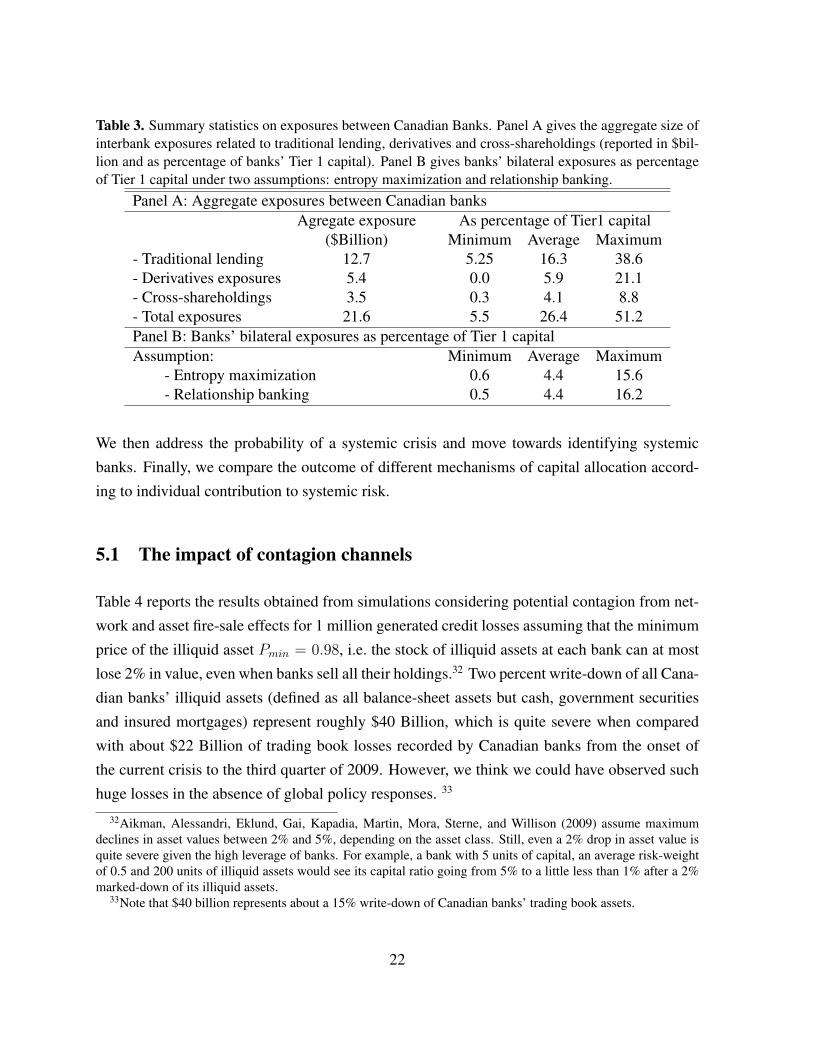
Table 3. Summary statistics on exposures between Canadian Banks. Panel A gives the aggregate size ofinterbank exposures related to traditional lending, derivatives and cross-shareholdings (reported in $bil-lion and as percentage of banks’ Tier 1 capital). Panel B gives banks’ bilateral exposures as percentageof Tier 1 capital under two assumptions: entropy maximization and relationship banking.

Panel A: Aggregate exposures between Canadian banksAgregate exposure As percentage of Tier1 capital

($Billion) Minimum Average Maximum- Traditional lending 12.7 5.25 16.3 38.6- Derivatives exposures 5.4 0.0 5.9 21.1- Cross-shareholdings 3.5 0.3 4.1 8.8- Total exposures 21.6 5.5 26.4 51.2Panel B: Banks’ bilateral exposures as percentage of Tier 1 capitalAssumption: Minimum Average Maximum

- Entropy maximization 0.6 4.4 15.6- Relationship banking 0.5 4.4 16.2

We then address the probability of a systemic crisis and move towards identifying systemic

banks. Finally, we compare the outcome of different mechanisms of capital allocation accord-

ing to individual contribution to systemic risk.

5.1 The impact of contagion channels

Table 4 reports the results obtained from simulations considering potential contagion from net-

work and asset fire-sale effects for 1 million generated credit losses assuming that the minimum

price of the illiquid asset Pmin = 0.98, i.e. the stock of illiquid assets at each bank can at most

lose 2% in value, even when banks sell all their holdings.32 Two percent write-down of all Cana-

dian banks’ illiquid assets (defined as all balance-sheet assets but cash, government securities

and insured mortgages) represent roughly $40 Billion, which is quite severe when compared

with about $22 Billion of trading book losses recorded by Canadian banks from the onset of

the current crisis to the third quarter of 2009. However, we think we could have observed such

huge losses in the absence of global policy responses. 33

32Aikman, Alessandri, Eklund, Gai, Kapadia, Martin, Mora, Sterne, and Willison (2009) assume maximumdeclines in asset values between 2% and 5%, depending on the asset class. Still, even a 2% drop in asset value isquite severe given the high leverage of banks. For example, a bank with 5 units of capital, an average risk-weightof 0.5 and 200 units of illiquid assets would see its capital ratio going from 5% to a little less than 1% after a 2%marked-down of its illiquid assets.

33Note that $40 billion represents about a 15% write-down of Canadian banks’ trading book assets.

22

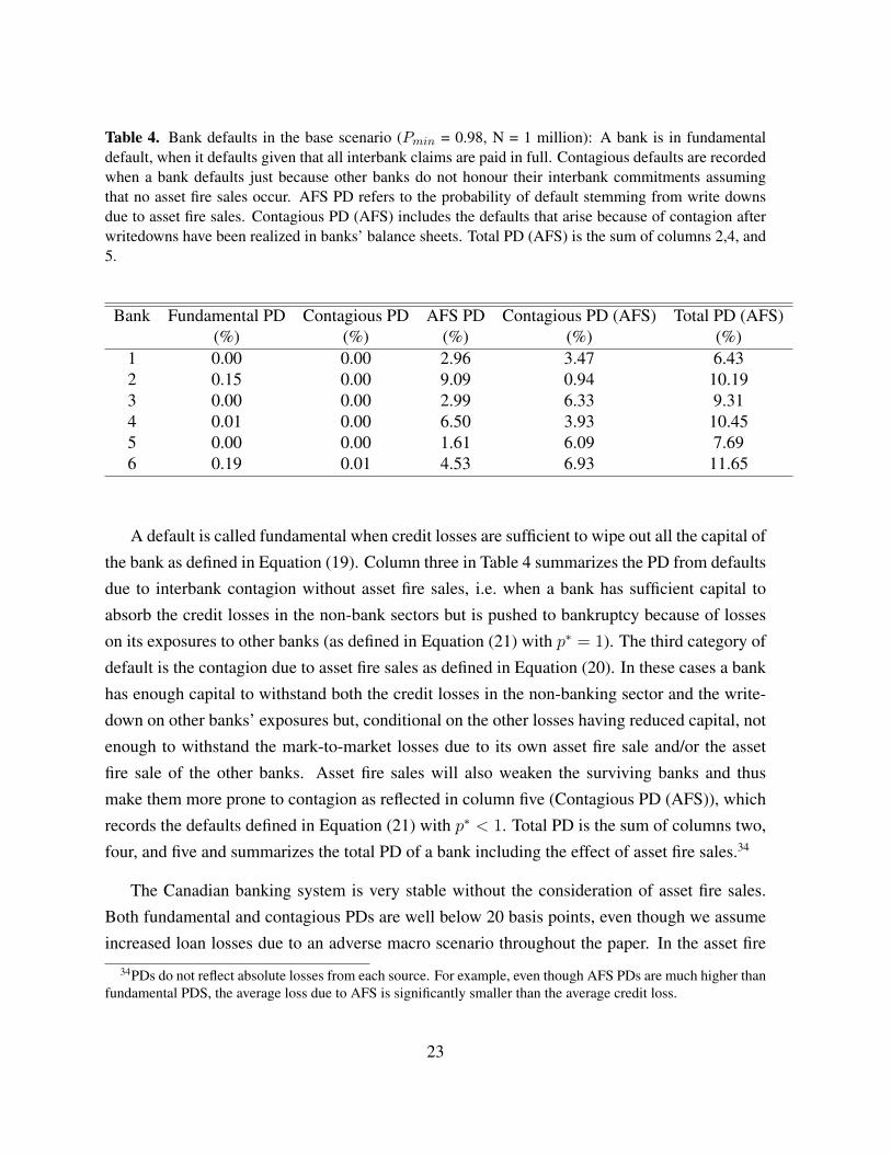
Table 4. Bank defaults in the base scenario (Pmin = 0.98, N = 1 million): A bank is in fundamentaldefault, when it defaults given that all interbank claims are paid in full. Contagious defaults are recordedwhen a bank defaults just because other banks do not honour their interbank commitments assumingthat no asset fire sales occur. AFS PD refers to the probability of default stemming from write downsdue to asset fire sales. Contagious PD (AFS) includes the defaults that arise because of contagion afterwritedowns have been realized in banks’ balance sheets. Total PD (AFS) is the sum of columns 2,4, and5.

Bank Fundamental PD Contagious PD AFS PD Contagious PD (AFS) Total PD (AFS)(%) (%) (%) (%) (%)

1 0.00 0.00 2.96 3.47 6.432 0.15 0.00 9.09 0.94 10.193 0.00 0.00 2.99 6.33 9.314 0.01 0.00 6.50 3.93 10.455 0.00 0.00 1.61 6.09 7.696 0.19 0.01 4.53 6.93 11.65

A default is called fundamental when credit losses are sufficient to wipe out all the capital of

the bank as defined in Equation (19). Column three in Table 4 summarizes the PD from defaults

due to interbank contagion without asset fire sales, i.e. when a bank has sufficient capital to

absorb the credit losses in the non-bank sectors but is pushed to bankruptcy because of losses

on its exposures to other banks (as defined in Equation (21) with p∗ = 1). The third category of

default is the contagion due to asset fire sales as defined in Equation (20). In these cases a bank

has enough capital to withstand both the credit losses in the non-banking sector and the write-

down on other banks’ exposures but, conditional on the other losses having reduced capital, not

enough to withstand the mark-to-market losses due to its own asset fire sale and/or the asset

fire sale of the other banks. Asset fire sales will also weaken the surviving banks and thus

make them more prone to contagion as reflected in column five (Contagious PD (AFS)), which

records the defaults defined in Equation (21) with p∗ < 1. Total PD is the sum of columns two,

four, and five and summarizes the total PD of a bank including the effect of asset fire sales.34

The Canadian banking system is very stable without the consideration of asset fire sales.

Both fundamental and contagious PDs are well below 20 basis points, even though we assume

increased loan losses due to an adverse macro scenario throughout the paper. In the asset fire

34PDs do not reflect absolute losses from each source. For example, even though AFS PDs are much higher thanfundamental PDS, the average loss due to AFS is significantly smaller than the average credit loss.

23

sale scenario, troubled banks want to maintain regulatory capital requirements by selling off

assets, which causes externalities for all other banks as asset prices fall. PDs increase and as

banks get weaker because of writedowns they also become more susceptible for contagion. We

find that banks 2, 4 and 6 have a higher risk of defaulting due to asset writedowns. While

banks 1, 3 and 5 are more likely to survive writedowns, losses to bank 3 and 5 weaken them

substantially so that they are more likely to default due to second round interbank contagion.

Overall, banks have PDs ranging from 6.43 to 11.65. Bank 1 and 5 stand out with the lowest

PDs while bank 6 has the highest one.

Remember that no government or central bank interventions to limit AFS are allowed in

the model to better measure the externalities imposed by more systemic banks on others. As a

result, the PDs of banks are likely much higher in our model than in a more realistic world where

central bank’s liquidity facilities and/or government measures would be put in place. Moreover,

these PDs are conditional on a very severe scenario. All things considered, the results shown in

Table 4 suggest that the Canadian banking system is very stable.

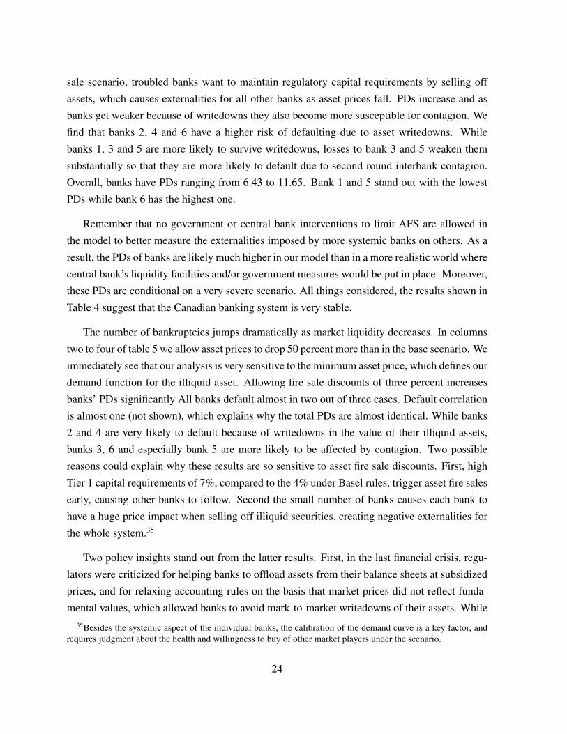
The number of bankruptcies jumps dramatically as market liquidity decreases. In columns

two to four of table 5 we allow asset prices to drop 50 percent more than in the base scenario. We

immediately see that our analysis is very sensitive to the minimum asset price, which defines our

demand function for the illiquid asset. Allowing fire sale discounts of three percent increases

banks’ PDs significantly All banks default almost in two out of three cases. Default correlation

is almost one (not shown), which explains why the total PDs are almost identical. While banks

2 and 4 are very likely to default because of writedowns in the value of their illiquid assets,

banks 3, 6 and especially bank 5 are more likely to be affected by contagion. Two possible

reasons could explain why these results are so sensitive to asset fire sale discounts. First, high

Tier 1 capital requirements of 7%, compared to the 4% under Basel rules, trigger asset fire sales

early, causing other banks to follow. Second the small number of banks causes each bank to

have a huge price impact when selling off illiquid securities, creating negative externalities for

the whole system.35

Two policy insights stand out from the latter results. First, in the last financial crisis, regu-

lators were criticized for helping banks to offload assets from their balance sheets at subsidized

prices, and for relaxing accounting rules on the basis that market prices did not reflect funda-

mental values, which allowed banks to avoid mark-to-market writedowns of their assets. While35Besides the systemic aspect of the individual banks, the calibration of the demand curve is a key factor, and

requires judgment about the health and willingness to buy of other market players under the scenario.

24

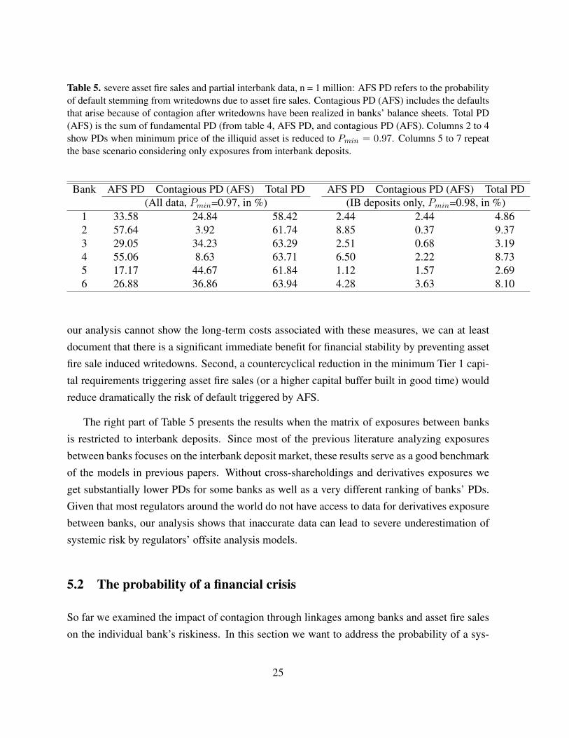
Table 5. severe asset fire sales and partial interbank data, n = 1 million: AFS PD refers to the probabilityof default stemming from writedowns due to asset fire sales. Contagious PD (AFS) includes the defaultsthat arise because of contagion after writedowns have been realized in banks’ balance sheets. Total PD(AFS) is the sum of fundamental PD (from table 4, AFS PD, and contagious PD (AFS). Columns 2 to 4show PDs when minimum price of the illiquid asset is reduced to Pmin = 0.97. Columns 5 to 7 repeatthe base scenario considering only exposures from interbank deposits.

Bank AFS PD Contagious PD (AFS) Total PD AFS PD Contagious PD (AFS) Total PD(All data, Pmin=0.97, in %) (IB deposits only, Pmin=0.98, in %)

1 33.58 24.84 58.42 2.44 2.44 4.862 57.64 3.92 61.74 8.85 0.37 9.373 29.05 34.23 63.29 2.51 0.68 3.194 55.06 8.63 63.71 6.50 2.22 8.735 17.17 44.67 61.84 1.12 1.57 2.696 26.88 36.86 63.94 4.28 3.63 8.10

our analysis cannot show the long-term costs associated with these measures, we can at least

document that there is a significant immediate benefit for financial stability by preventing asset

fire sale induced writedowns. Second, a countercyclical reduction in the minimum Tier 1 capi-

tal requirements triggering asset fire sales (or a higher capital buffer built in good time) would

reduce dramatically the risk of default triggered by AFS.

The right part of Table 5 presents the results when the matrix of exposures between banks

is restricted to interbank deposits. Since most of the previous literature analyzing exposures

between banks focuses on the interbank deposit market, these results serve as a good benchmark

of the models in previous papers. Without cross-shareholdings and derivatives exposures we

get substantially lower PDs for some banks as well as a very different ranking of banks’ PDs.

Given that most regulators around the world do not have access to data for derivatives exposure

between banks, our analysis shows that inaccurate data can lead to severe underestimation of

systemic risk by regulators’ offsite analysis models.

5.2 The probability of a financial crisis

So far we examined the impact of contagion through linkages among banks and asset fire sales

on the individual bank’s riskiness. In this section we want to address the probability of a sys-

25

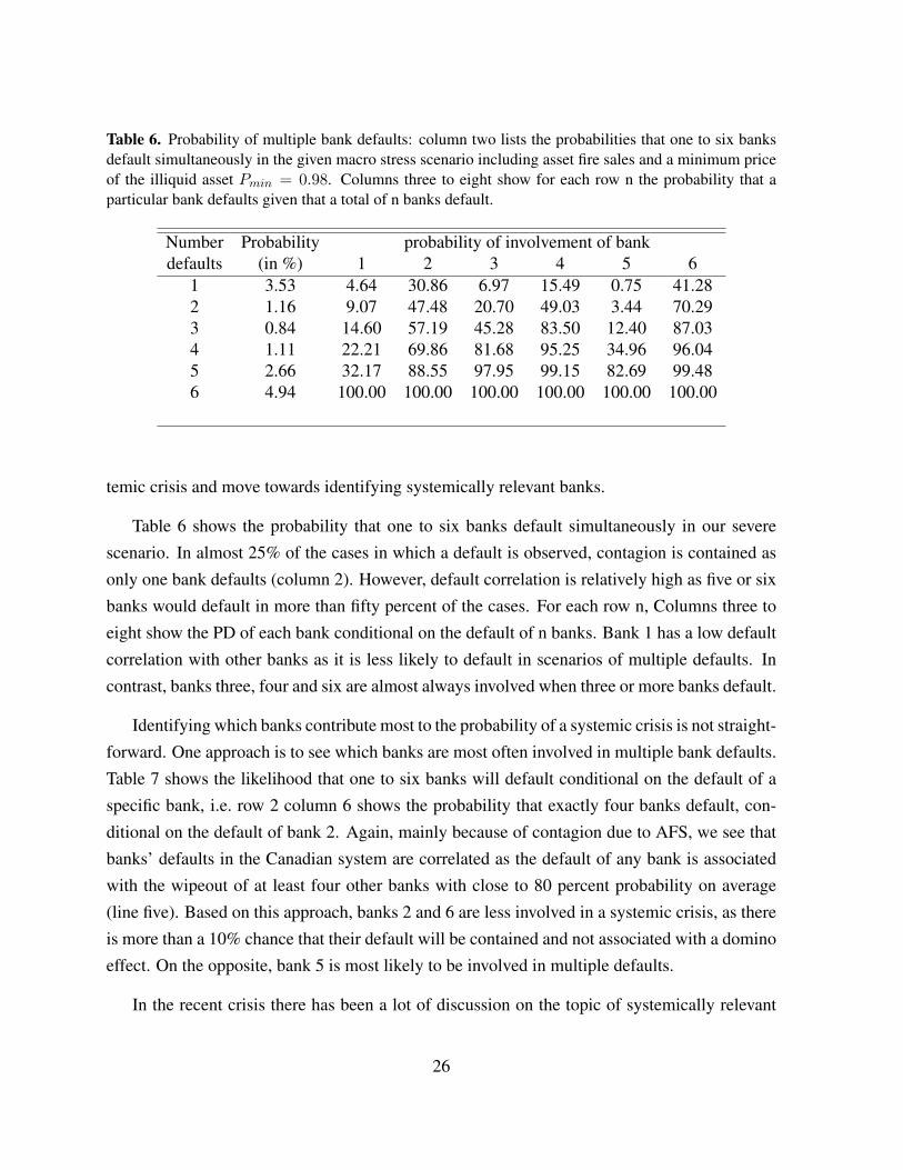
Table 6. Probability of multiple bank defaults: column two lists the probabilities that one to six banksdefault simultaneously in the given macro stress scenario including asset fire sales and a minimum priceof the illiquid asset Pmin = 0.98. Columns three to eight show for each row n the probability that aparticular bank defaults given that a total of n banks default.

Number Probability probability of involvement of bankdefaults (in %) 1 2 3 4 5 6

1 3.53 4.64 30.86 6.97 15.49 0.75 41.282 1.16 9.07 47.48 20.70 49.03 3.44 70.293 0.84 14.60 57.19 45.28 83.50 12.40 87.034 1.11 22.21 69.86 81.68 95.25 34.96 96.045 2.66 32.17 88.55 97.95 99.15 82.69 99.486 4.94 100.00 100.00 100.00 100.00 100.00 100.00

temic crisis and move towards identifying systemically relevant banks.

Table 6 shows the probability that one to six banks default simultaneously in our severe

scenario. In almost 25% of the cases in which a default is observed, contagion is contained as

only one bank defaults (column 2). However, default correlation is relatively high as five or six

banks would default in more than fifty percent of the cases. For each row n, Columns three to

eight show the PD of each bank conditional on the default of n banks. Bank 1 has a low default

correlation with other banks as it is less likely to default in scenarios of multiple defaults. In

contrast, banks three, four and six are almost always involved when three or more banks default.

Identifying which banks contribute most to the probability of a systemic crisis is not straight-

forward. One approach is to see which banks are most often involved in multiple bank defaults.

Table 7 shows the likelihood that one to six banks will default conditional on the default of a

specific bank, i.e. row 2 column 6 shows the probability that exactly four banks default, con-

ditional on the default of bank 2. Again, mainly because of contagion due to AFS, we see that

banks’ defaults in the Canadian system are correlated as the default of any bank is associated

with the wipeout of at least four other banks with close to 80 percent probability on average

(line five). Based on this approach, banks 2 and 6 are less involved in a systemic crisis, as there

is more than a 10% chance that their default will be contained and not associated with a domino

effect. On the opposite, bank 5 is most likely to be involved in multiple defaults.

In the recent crisis there has been a lot of discussion on the topic of systemically relevant

26

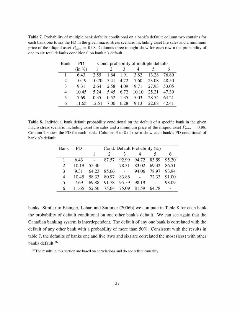
Table 7. Probability of multiple bank defaults conditional on a bank’s default: column two contains foreach bank one to six the PD in the given macro stress scenario including asset fire sales and a minimumprice of the illiquid asset Pmin = 0.98. Columns three to eight show for each row n the probability ofone to six total defaults conditional on bank n’s default.

Bank PD Cond. probability of multiple defaults(in %) 1 2 3 4 5 6

1 6.43 2.55 1.64 1.91 3.82 13.28 76.802 10.19 10.70 5.41 4.72 7.60 23.08 48.503 9.31 2.64 2.58 4.09 9.71 27.93 53.054 10.45 5.24 5.45 6.72 10.10 25.21 47.305 7.69 0.35 0.52 1.35 5.03 28.54 64.216 11.65 12.51 7.00 6.28 9.13 22.68 42.41

Table 8. Individual bank default probability conditional on the default of a specific bank in the givenmacro stress scenario including asset fire sales and a minimum price of the illiquid asset Pmin = 0.98:Column 2 shows the PD for each bank. Columns 3 to 8 of row n show each bank’s PD conditional ofbank n’s default.

Bank PD Cond. Default Probability (%)1 2 3 4 5 6

1 6.43 - 87.57 92.99 94.72 83.59 95.202 10.19 55.30 - 78.31 83.02 69.32 86.513 9.31 64.23 85.66 - 94.06 78.97 93.944 10.45 58.33 80.97 83.86 - 72.33 91.005 7.69 69.88 91.78 95.59 98.19 - 98.096 11.65 52.56 75.64 75.09 81.59 64.78 -

banks. Similar to Elsinger, Lehar, and Summer (2006b) we compute in Table 8 for each bank

the probability of default conditional on one other bank’s default. We can see again that the

Canadian banking system is interdependent. The default of any one bank is correlated with the

default of any other bank with a probability of more than 50%. Consistent with the results in

table 7, the defaults of banks one and five (two and six) are correlated the most (less) with other

banks default.36

36The results in this section are based on correlations and do not reflect causality.

27

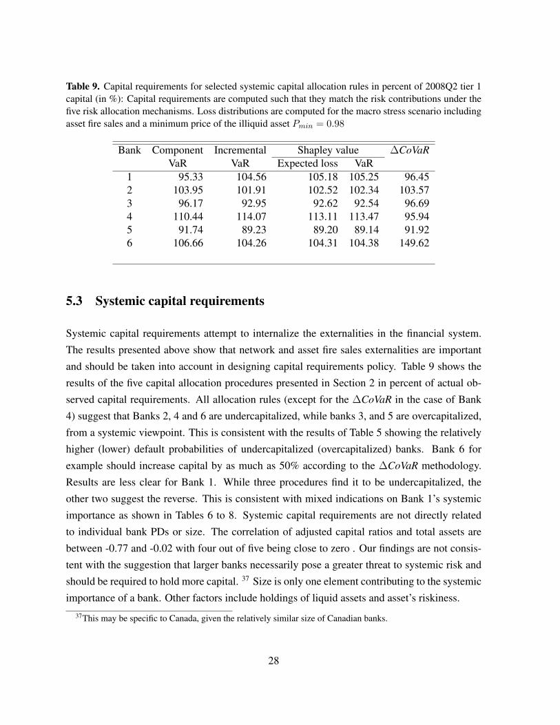
Table 9. Capital requirements for selected systemic capital allocation rules in percent of 2008Q2 tier 1capital (in %): Capital requirements are computed such that they match the risk contributions under thefive risk allocation mechanisms. Loss distributions are computed for the macro stress scenario includingasset fire sales and a minimum price of the illiquid asset Pmin = 0.98

Bank Component Incremental Shapley value ∆CoVaRVaR VaR Expected loss VaR

1 95.33 104.56 105.18 105.25 96.452 103.95 101.91 102.52 102.34 103.573 96.17 92.95 92.62 92.54 96.694 110.44 114.07 113.11 113.47 95.945 91.74 89.23 89.20 89.14 91.926 106.66 104.26 104.31 104.38 149.62

5.3 Systemic capital requirements

Systemic capital requirements attempt to internalize the externalities in the financial system.

The results presented above show that network and asset fire sales externalities are important

and should be taken into account in designing capital requirements policy. Table 9 shows the

results of the five capital allocation procedures presented in Section 2 in percent of actual ob-

served capital requirements. All allocation rules (except for the ∆CoVaR in the case of Bank

4) suggest that Banks 2, 4 and 6 are undercapitalized, while banks 3, and 5 are overcapitalized,

from a systemic viewpoint. This is consistent with the results of Table 5 showing the relatively

higher (lower) default probabilities of undercapitalized (overcapitalized) banks. Bank 6 for

example should increase capital by as much as 50% according to the ∆CoVaR methodology.

Results are less clear for Bank 1. While three procedures find it to be undercapitalized, the

other two suggest the reverse. This is consistent with mixed indications on Bank 1’s systemic

importance as shown in Tables 6 to 8. Systemic capital requirements are not directly related

to individual bank PDs or size. The correlation of adjusted capital ratios and total assets are

between -0.77 and -0.02 with four out of five being close to zero . Our findings are not consis-

tent with the suggestion that larger banks necessarily pose a greater threat to systemic risk and

should be required to hold more capital. 37 Size is only one element contributing to the systemic

importance of a bank. Other factors include holdings of liquid assets and asset’s riskiness.

37This may be specific to Canada, given the relatively similar size of Canadian banks.

28

Table 10. Individual bank default probability under selected macroprudential capital allocation rules(in %). Default probabilities are computed for the macro stress scenario including asset fire sales and aminimum price of the illiquid asset Pmin = 0.98.

Bank Observed Basel Component Incremental Shapley value ∆CoVaRcapital equal VaR VaR Expected loss VaR

1 6.43 9.05 6.60 3.91 3.75 3.73 7.532 10.19 9.97 7.68 8.15 7.91 7.97 8.933 9.31 8.91 8.34 8.82 8.87 8.91 10.574 10.45 9.04 6.72 5.77 5.91 5.85 11.975 7.70 7.73 7.55 7.76 7.73 7.74 9.476 11.65 10.53 8.28 8.49 8.44 8.43 2.42Average 9.29 9.21 7.53 7.15 7.10 7.11 8.48

Compared to the observed capital levels, all systemic capital allocations reduce the default

probability of the average bank. Table 10 shows the default probabilities of the six banks under

the observed capital ratio, the ”Basel equal” benchmark, as well as under the five macropru-

dential allocations. The Component VaR method creates relatively homogeneous PDs for all

banks, increasing the likelihood of default for bank 1, but making banks 2 to 6 less prone to

default. The incremental VaR and Shapley allocations leave bank 3 and 5’s PD relatively un-

changed but reduce the PD for banks 1 and 4 and 6 substantially. The ∆CoVaR reduces Bank 6

PD dramatically.

All five systemic capital requirements reduce risk in the banking system. Table 11 presents

the probability of multiple bank defaults for the five capital allocation rules. Especially incre-

mental VaR and the Shapley value allocations reduce the probability of multiple bank failures

significantly. Under Shapley value based capital allocations the probability of five or six banks

defaulting can be reduced from 7.6%, which is based on current banks’ capital levels, to 5.5%.

This corresponds to a 27% reduction in the probability of a financial crisis.

Table 12 computes the expected loss under the different capital allocation mechanisms. The

expected loss equals the fair deposit insurance premium assuming that all bank liabilities are

insured. We can again see that systemic capital requirements can substantially reduce bank risk

compared to capital levels under the current regulatory regime.

29

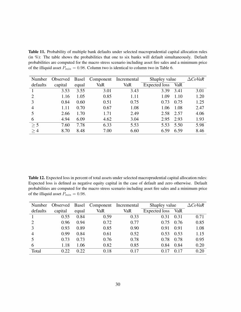
Table 11. Probability of multiple bank defaults under selected macroprudential capital allocation rules(in %): The table shows the probabilities that one to six banks will default simultaneously. Defaultprobabilities are computed for the macro stress scenario including asset fire sales and a minimum priceof the illiquid asset Pmin = 0.98. Column two is identical to column two in Table 6.

Number Observed Basel Component Incremental Shapley value ∆CoVaRdefaults capital equal VaR VaR Expected loss VaR1 3.53 3.55 3.01 3.43 3.39 3.41 3.012 1.16 1.05 0.85 1.11 1.09 1.10 1.203 0.84 0.60 0.51 0.75 0.73 0.75 1.254 1.11 0.70 0.67 1.08 1.06 1.08 2.475 2.66 1.70 1.71 2.49 2.58 2.57 4.066 4.94 6.09 4.62 3.04 2.95 2.93 1.93≥ 5 7.60 7.78 6.33 5.53 5.53 5.50 5.98≥ 4 8.70 8.48 7.00 6.60 6.59 6.59 8.46

Table 12. Expected loss in percent of total assets under selected macroprudential capital allocation rules:Expected loss is defined as negative equity capital in the case of default and zero otherwise. Defaultprobabilities are computed for the macro stress scenario including asset fire sales and a minimum priceof the illiquid asset Pmin = 0.98.

Number Observed Basel Component Incremental Shapley value ∆CoVaRdefaults capital equal VaR VaR Expected loss VaR1 0.55 0.84 0.59 0.33 0.31 0.31 0.712 0.96 0.94 0.72 0.77 0.75 0.76 0.853 0.93 0.89 0.85 0.90 0.91 0.91 1.084 0.99 0.84 0.61 0.52 0.53 0.53 1.155 0.73 0.73 0.76 0.78 0.78 0.78 0.956 1.18 1.06 0.82 0.85 0.84 0.84 0.20Total 0.22 0.22 0.18 0.17 0.17 0.17 0.20

30

6 Conclusions

One feature of the macroprudential approach is to threat aggregate risk in the financial system

as being dependent on the collective actions of financial institutions and markets. In this paper,

we use a model which explicitly considers contagion effects through network and asset fire sale

externalities and sheds light on their importance. We generate an aggregate loss distribution of

the banking system using a balance-sheet stress-testing model that integrate credit and market

liquidity risk in a network of exposures between banks. To better capture the likelihood of

contagion default, we use a unique sample of the Canadian banking system, which includes

detailed information on interbank linkages including OTC derivatives.

We compare alternative mechanisms of allocating systemic risk to individual institutions.

Importantly, we follow an iterative procedure to solve for a fixed point for which capital alloca-

tions are consistent with the contributions of each bank to the total risk of the banking system,

under the proposed capital allocations. We find that financial stability can be enhanced substan-

tially by implementing a system perspective on bank regulation. The resulting new allocations

of capital reduce significantly both the default probabilities of individual institutions and the

probability of multiple bank defaults.

We also find that ignoring our information on derivatives and cross shareholdings gives us a

different picture of individual bank risk with potential important implications for systemic risk.

This speaks to the importance of getting better information about exposures between financial

institutions

Our results are of course dependent on the calibration of the model used in this paper and

the severity of the underlying scenario, and reflect the features of the Canadian banking system.

However, we think the approach we propose could be useful, combined with expert judgment,

in guiding the implementation of a macroprudential approach to financial system regulation.

31

References

Adrian, Tobias, and Markus K. Brunnermeier, 2009, CoVaR, working paper, Princeton Univer-sity.

Aikman, David, Piergiorgio Alessandri, Bruno Eklund, Prasanna Gai, Sujit Kapadia, ElizabethMartin, Nada Mora, Gabriel Sterne, and Matthew Willison, 2009, Funding Liquidity Risk ina Quantitative Model of Systemic Stability, .

Allen, Frank, and Douglas Gale, 1994, Limited Market Participation and Volatility of AssetPrices, American Economic Review 84, 933–955.

Allen, Frank, and Douglas Gale, 2000, Financial Contagion, Journal of Political Economy 108,1–33.

Bae, Kee-Hong, Andrew G. Karolyi, and Rene M. Stulz, 2003, A New Approach to MeasuringFinancial Contagion, The Review of Financial Studies pp. 717–763.

Blien, Uwe, and Friedrich Graef, 1997, Entropy Optimizing Methods for the Estimation ofTables, in Ingo Balderjahn, Rudolf Mathar, and Martin Schader, eds.: Classification, DataAnalysis, and Data Highways (Springer Verlag, Berlin ).

Borio, Claudio, 2002, Towards a Macro-Prudential Framework for Financial Supervision andRegulation?, CESifo Lecture, Summer Institute: Banking Regulation and Financial Stability,Venice.

Cifuentes, Rodrigo, Hyun Song Shin, and Gianluigi Ferrucci, 2005, Liquidity Risk and Conta-gion, Journal of European Economic Association 3, 556–566.

Credit Suisse, 1997, Credit Risk+: A Credit Risk Management Framework, .

Crouhy, Michel, Dan Galai, and Robert Mark, 2000, A Comparative Analysis of Current CreditRisk Models, Journal of Banking and Finance 24, 59117.

David, Alexander, and Alfred Lehar, 2009, Systemic Risk as Renegotiation Breakdown, work-ing paper.

Denault, Michel, 2001, Coherent allocation of risk capital, Journal of Risk 4, 1–34.

Eisenberg, Larry, and Thomas Noe, 2001, Systemic Risk in Financial Systems, ManagementScience 47, 236–249.

Elsinger, Helmut, Alfred Lehar, and Martin Summer, 2006a, Risk Assessment for BankingSystems, Management Science 52, 1301–1314.

32

Elsinger, Helmut, Alfred Lehar, and Martin Summer, 2006b, Systemically Important Banks: AnAnalysis for the European Banking System, International Economics and Economic Policy3, 73–89.

Forbes, Kristin J., and Roberto Rigobon, 2002, No Contagion, Only Interdependence: Measur-ing Stock Market Comovements, Journal of Finance pp. 2223–2261.

Gauthier, Celine, and St-Amant, 2005, Analyzing the Evolution of Financial Instability Risk,Bank of Canada Financial System Review December, 47–53.

Geithner, Timothy F., 2009, Treasury Secretary Timothy F. Geithner Written Testimony beforethe House Financial Services Committee, US department of the treasury.

Gul, Faruk, 1989, Bargaining Foundations of Shapley Value, Econometrica 57, 81–96.

Jorion, Philippe, 2007, Value-at-Risk. (McGraw-Hill) third edn.

Kalkbrener, Michael, 2005, An Axiomatic Approach to Capital Allocation, Mathematical Fi-nance 15, 425–437.

Krishnamurthy, Arvind, 2009, Amplification Mechanisms in Liquidity Crises, American Eco-nomic Review p. forthcoming.

Lalonde, Don Colettiand Rene, Miroslav Misina, Dirk Muir, Pierre St-Amant, and DavidTessier, 2008, Bank of Canada Participation in the 2007 FSAP Macro Stress-Testing Ex-ercise, Bank of Canada Financial System Review June, 51–59.

Misina, Miroslav, and David Tessier, 2007, Sectoral Default Rates under Stress: The Impor-tance of non-Linearities, Bank of Canada Financial System Review June, 49–54.

Misina, Miroslav, David Tessier, and Shubhasis Dey, 2006, Stress Testing the Corporate LoansPortfolio of the Canadian Banking Sector, Bank of Canada Working Paper No. 2006-47.

Sheldon, George, and Martin Maurer, 1998, Interbank Lending and Systemic Risk: an Empiri-cal Analysis for Switzerland, Swiss Journal of Economics and Statistics 134, 685–704.

Shin, Hyun Song, 2008, Risk and Liquidity in a System Context, working paper, PrincetonUniversity.

Tarashev, Nikola, Claudio Borio, and Kostas Tsatsaronis, 2009, The systemic importance offinancial institutions, BIS quarterly review September, 75–87.

Upper, Christian, 2007, Using counterfactual simulations to assess the danger of contagion ininterbank markets, BIS Working Paper no 234.

Upper, Christian, and Andreas Worms, 2004, Estimating Bilateral Exposures in the GermanInterbank Market: Is there a Danger of Contagion, European Economic Review 48, 99–133.

33

Wells, Simon, 2002, UK Interbank Exposures: systemic risk implications, Financial StabilityReview 13, 175–182.

34