Computer Communications 46 (2014) 54–65

Contents lists available at ScienceDirect

Computer Communications

journal homepage: www.elsevier .com/ locate/comcom

Minimizing the number of mobile chargers for large-scale wirelessrechargeable sensor networks q

http://dx.doi.org/10.1016/j.comcom.2014.03.0010140-3664/� 2014 Elsevier B.V. All rights reserved.

q A preliminary version of this paper appeared in [1].⇑ Corresponding author.

E-mail addresses: dhpphd2003@gmail.com (H. Dai), wuxb@nju.edu.cn (X. Wu),gchen@nju.edu.cn (G. Chen), ljxu83@gmail.com (L. Xu), slin@temple.edu (S. Lin).

Haipeng Dai ⇑, Xiaobing Wu, Guihai Chen, Lijie Xu, Shan LinState Key Laboratory for Novel Software Technology, Nanjing University, Nanjing 210023, PR China

a r t i c l e i n f o a b s t r a c t

Article history:Available online 12 March 2014

Keywords:Wireless rechargeable sensor networksMobile chargingTwo-dimension

Traditional wireless sensor networks (WSNs) are constrained by limited battery energy that powers thesensor nodes, which impedes the large-scale deployment of WSNs. Wireless power transfer technologyprovides a promising way to solve this problem. With such novel technology, recent works propose touse a single mobile charger (MC) traveling through the network fields to replenish energy to every sensornode so that none of the nodes will run out of energy. These algorithms work well in small-scale net-works. In large-scale networks, these algorithms, however, do not work efficiently, especially when theamount of energy the MC can provide is limited. To address this issue, multiple MCs can be used. In thispaper, we investigate the minimum MCs problem (MinMCP) for two-dimensional (2D) wireless recharge-able sensor networks (WRSNs), i.e., how to find the minimum number of energy-constrained MCs anddesign their recharging routes in a 2D WRSN such that each sensor node in the network maintains con-tinuous work, assuming that the energy consumption rate for all sensor nodes are identical. By reductionfrom the Distance Constrained Vehicle Routing Problem (DVRP), we prove that MinMCP is NP-hard. Thenwe propose approximation algorithms for this problem. Finally, we conduct extensive simulations to val-idate the effectiveness of our algorithms.

� 2014 Elsevier B.V. All rights reserved.

1. Introduction

Wireless sensor networks (WSNs) have been widely used forstructural health monitoring, scientific exploration, environmentalmonitoring, target tracking, etc. As sensor nodes in traditionalWSNs are powered by batteries, the limited battery energy is con-sidered as a major deployment barrier for large-scale WSNs. Toelongate the lifetime of WSNs, many approaches have been pro-posed to harvest ambient energy from their surroundings such assolar energy [2], vibration energy [3], and wind energy [4]. How-ever, due to the time-varying nature of renewable energy re-sources, the success of these methods remains very limited inpractice.

The recent breakthroughs in wireless power transfer technology[5], which allow energy to be transferred from one storage deviceto another via wireless with reasonable efficiency, has provided apromising way to solve this problem. Since wireless rechargingcan guarantee the continuous power supply and is insensitive tothe neighboring environment, it has found many applications

including RFIDs [6], sensors [7], cell phones [8], laptops [9], vehi-cles [10], smart grids [11] and civil structures monitoring [12].With the novel technology, recent studies [12–18,1] propose toemploy a mobile charger (MC) to replenish energy to sensor nodesin wireless rechargeable sensor networks (WRSNs) [19–21] so thatnone of them in the network will run out of energy. Typically, theMC periodically traverses every node in the network and stays nearevery node for a short period to recharge it. Research results dem-onstrate that this approach works well for small-scale networks.For large-scale wireless sensor networks, a single mobile chargermay not be enough. This is because the MC may not carry sufficientenergy to recharge every node in a large-scale network on a singletour. Therefore, the MC needs to return to the base station afterrecharging a part of the network. As a result, single MC rechargingalgorithms become invalid and continuous working of sensornodes can no longer be guaranteed.

To recharge a large-scale sensor network, it is necessary to usemultiple energy constrained mobile chargers. In this work, weinvestigate the minimum mobile charger problem for wireless sen-sor networks. That is, how to find the minimum number of energy-constrained MCs as well as their routes to recharge a given WRSNsuch that each sensor node in the WRSN can work continuously. Inour problem settings, the energy consumption rate for all sensornodes are identical, which is a practical assumption for many

H. Dai et al. / Computer Communications 46 (2014) 54–65 55

applications as will be elaborated. This problem is highly challeng-ing as we should jointly consider the energy constraints of MCs andthe time-sensitive charging requirements of sensor nodes whendetermining the routes of MCs. We prove the NP-hardness of thisproblem and propose efficient approximation algorithms to solveit. Zhang et al. [22] also employed multiple energy-constrainedMCs. However, their work focuses on only one-dimensional (1D)sensor networks, and their goal is to maximize the ratio of theamount of payload energy to the overhead energy. Our solutionis designed for two-dimensional (2D) sensor networks, and con-centrates on an entirely different problem compared with [22].

The contributions of this work are as follows.

� We are the first to consider the minimum mobile chargers prob-lem (MinMCP) in general 2D WRSNs, i.e., how to find the mini-mum number of energy-constrained MCs and their rechargingroutes given a 2D WRSN, so as to keep the network runningforever.� We prove that MinMCP is NP-hard, and propose approximation

algorithms to address MinMCP. Particularly, we first considerthe relaxed version of MinMCP, which is named MinMCP-R,and propose an approximation algorithm to address it. Further-more, we present approximation algorithms to MinMCP basedon the results obtained for MinMCP-R.� We conduct extensive simulations to verify our analytical find-

ings. The simulation results demonstrate the effectiveness ofour schemes.

The remainder of the paper is organized as follows. In Section 2, weinvestigate some related works. We present preliminaries and back-ground in Section 3. In Section 4, we first formulate the problemand investigate its hardness. Then we propose approximation algo-rithms and conduct performance analysis respectively. Section 5discusses how to extend our work to general cases. Experimentalresults are presented in Section 6 before we conclude the paper inSection 7.

Mobile Charger (MC) Sensor Node

Base Sta�on (BS)

Fig. 1. Illustration of the network model.

2. Related work

In this section, we review some related works in terms of mo-bile charging problems where a single or multiple MCs are used.

There has emerged a considerable amount of work studyinghow to use one single MC to enhance the performances of WRSNs.In terms of data routing performance, Tong et al. [13] investigatedthe impact of wireless charging technology on data routing anddeployment of sensor networks where a single MC is applied. Amore practical scheme jointly considering routing and chargingwas reported in [15]. It aimed to maximize the network lifetimeunder practical constraints such as dynamic and unreliable com-munication environment, limited charging capability and hetero-geneous node attributes. Other works were interested in theimpact of mobile charging on the efficiency of data gathering. Shiet al. [14] employed an MC to periodically travel inside the sensornetwork to charge sensor nodes, and tried to minimize the aggre-gate charging time and travel time. By [23,24], a mobile chargerwas used to serve not only as an energy transporter that chargesstationary sensors, but also as a data collector. In addition, Xieet al. [25] studied the problem of co-locating the mobile base sta-tion on the wireless charging vehicle to minimize energy consump-tion of the entire system while guaranteeing that none of thesensor nodes will run out of energy. Still others concentrated onstochastic event capture issues. Dai et al. [18] considered two clo-sely related subproblems of mobile charging for stochastic eventcapture. One is how to choose the nodes for charging and decidethe charging time for each of them, and the other is how to best

schedule the nodes’ activation schedules according to their re-ceived energy. Their goal is to maximize the overall quality ofmonitoring.

Besides the above concerns on traditional performances of sen-sor networks, some literature paid attention to practical issues re-lated to the MC. Fu et al. [26] focused on minimizing the chargingdelay of the MC, an RFID-reader, by planning its optimal movementand charging strategy. While most existing works on the mobilecharging problem mainly concentrated on the optimal offline pathplanning for the MC, He et al. [27] considered the on-demand mo-bile charging problem, i.e., how to dynamically plan the path forthe MC where the charging requests from sensor nodes come ran-domly. Li et al. [16] tried to maximize the number of sensor nodesto be charged by using a single MC with limited energy, which isdifferent from the above schemes that assume the employed MChas unbounded energy.

In order to charge a large-scale WRSN, multiple MCs are neededconsidering their energy constraint. Zhang et al. [22] proposed theonly scheme employed multiple energy-constrained MCs to collab-oratively charge a linear WSN. MCs are allowed to charge eachother. Their goal is to maximize the energy efficiency of charging,which is totally different from ours.

3. Problem statement

3.1. Network model

We assume that there is a collection of rechargeable sensornodes distributed over a 2D region. A base station (BS) serves notonly as a data sink, but also as an energy source of the networkby periodically dispatching MCs to charge the sensor nodes, asillustrated in Fig. 1. Let G ¼ ðV ; EÞ represent the topology of sensornodes and the BS. Let vBS 2 V denote the BS, and J ¼ V n vBS ðjJj ¼ nÞbe the set of sensor nodes. Denote by wði; jÞ the time cost for MCstraveling from a sensor node v i to another sensor node v j, whichwe call the edge weight. Notice that wði; jÞ includes neither thecharging time of MCs at the sensor node v i nor that at the sensornode v j. We assume that G is complete, and the edge weights forma metric space W, namely, they are symmetric and satisfy the tri-angle inequality. To be specific, we have wði; jÞ ¼ wðj; iÞ andwði; jÞ 6 wði; kÞ þwðk; jÞ for arbitrary sensor nodes v i;v j and vk.We emphasize that this assumption is without loss of generalitybecause an MC can always travel along the shortest path betweenany two sensor nodes (e.g., if wði; jÞ > wði; kÞ þwðk; jÞ, an MC willprefer to travel from i to j by passing by k, which results in an

56 H. Dai et al. / Computer Communications 46 (2014) 54–65

equivalent edge weight between i and j;w0ði; jÞ ¼ wði; kÞ þwðk; jÞ),which leads to inherent triangle inequality among nodes.

Every sensor node has a battery capacity of Emax, and needs aminimum energy Emin to be operational. We assume that theenergy consumption rate is constant and uniform for all sensornodes, and is denoted by pw. This assumption holds for a numberof scenarios. For example, Jiang et al. [28] studied wireless powertransmission for sensor nodes buried inside concrete. These sensornodes collect valuable volumetric data related to the health of astructure, and wirelessly transmit the data to a data collectionreceiver directly [29]. As their transmitting power is uniform, theenergy consumptions of the sensor nodes are identical to eachother. In [12][30], a civil structure is instrumented with sensornodes capable of being charged wirelessly by a mobile helicopter,which also serves as a data collector. Thus, hop-by-hop data trans-missions are no longer needed, and the energy consumptions canbe conserved and balanced on sensor nodes. In addition, RFID sen-sors in Wireless Identification and Sensing Platform (WISP)[26,31,32] typically consume energy at the same rate, and theycan be wirelessly charged by a mobile charger [33].

A summary of the notations in this paper is given in Table 1.

3.2. Charging model

Suppose that a fully charged MC k starts from the BS and visitsevery node of a subset of sensor nodes Sk # J exactly once andcharges them. The MC k spends sk

i units of time in charging a nodev i. Denote the tour of the MC k by Pk ¼ ðp0;p1; . . . ;pjSk j;pjSk jþ1Þwhere p0 ¼ pjSk jþ1 ¼ vBS and fpigjSk j

i¼1 ¼ Sk. Consequently, the timethe MC k takes to travel along Pk is given by sk

P ¼ RjSk ji¼0wðpi;piþ1Þ.

Table 1Notations used.

Symbol Meaning

wði; jÞ Time cost for MCs traveling from node v i to v j

Emax Battery capacity for all sensor nodesEmin Minimum energy for sensor nodes to be operationalpw Energy consumption rate for all sensor nodesM Set of tours of all MCssk

iCharging time allocated to node v i by the MC k

skP

Travel time of the MC k

skvac

Vacation time of the MC k

scvac Minimum required vacation time for MCs

sk Time period of recharge schedule for the MC k

U Energy transfer rate of MCsB Battery capacity of MCsgC Working Power of MCs for TravelinggT Working Power of MCs for Charging

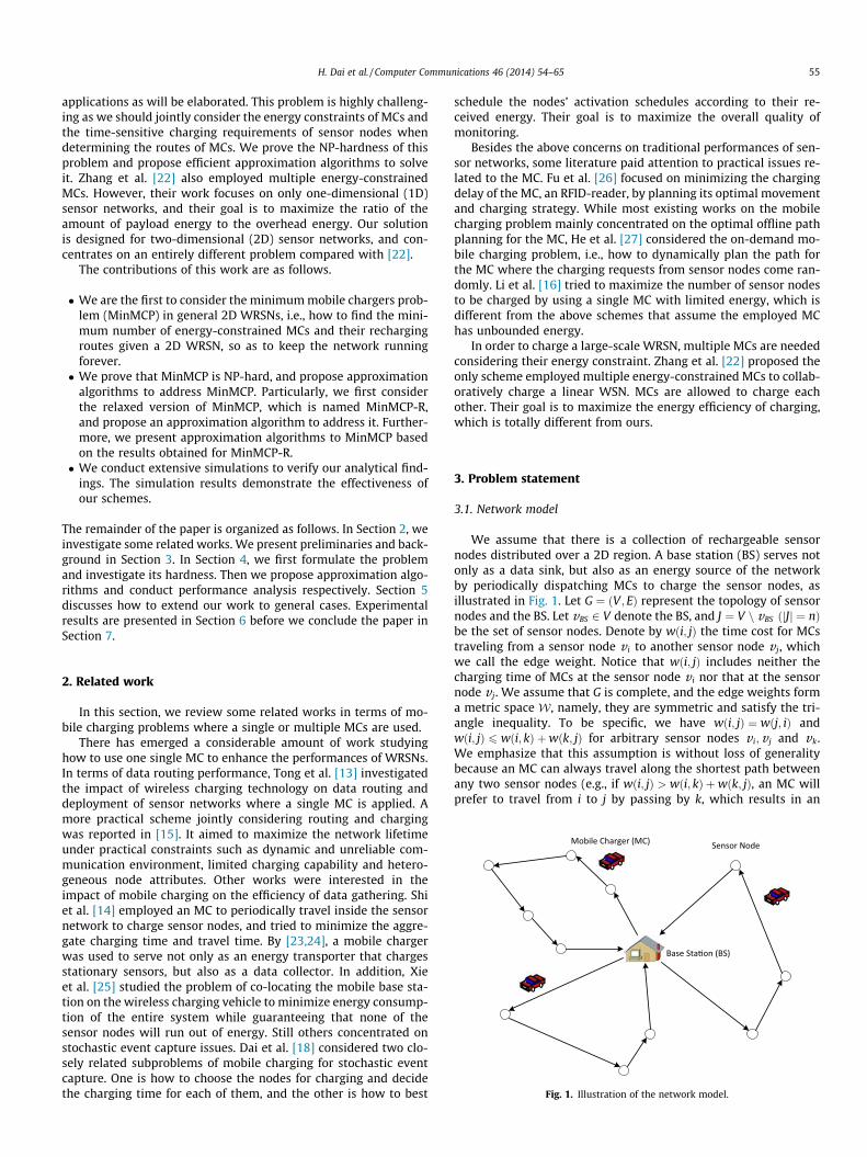
Fig. 2. Illustration of rene

Further, let M be the set of tours of all MCs, which means thatPk 2M and k 2 ½jMj� for any MC k.

After finishing the charging, The MC k returns to the BS to beserviced (e.g., replacing or recharging its battery) and gets readyfor the next trip. This period is called vacation time, and is denotedas sk

vac. We demand that skvac for any MC k should not be smaller

than a given constant value scvac , i.e.,

skvac P sc

vac ðk 2 ½jMj�Þ; ð1Þ

in order to meet the requirements of most applications. The MC krepeats its recharge schedule every period of time sk, which consistsof charging time, travel time and vacation time, i.e.,

sk ¼ skP þ sk

vac þ Rv i2Sksk

i ðk 2 ½jMj�Þ: ð2Þ

Let U ðU > pwÞ be the energy transfer rate of an MC during charging.To ensure that each sensor node maintains continuous work and thecharging cost of an MC is minimized, the renewable energy cycle ofeach sensor node should be guaranteed [14]. In particular, the en-ergy level of a sensor node v i 2 J exhibits a renewable energy cycleif it satisfies the following two requirements: (i) it starts and endswith the same energy level over a period of sk; and (ii) it never fallsbelow Emin. Mathematically, the following two conditions should besatisfied.

sk � pw ¼ ski � U ðk 2 ½jMj�;v i 2 SkÞ; ð3Þ

Emax � ðsk � ski Þ � pw P Emin ðk 2 ½jMj�; v i 2 SkÞ: ð4Þ

The first equation indicates that the amount of energy charged to anode v i during si must be equal to that consumed by v i in a sche-dule period, and the second inequality is obtained by consideringthe lowest energy level of the node.

We take Fig. 2 as an example. The energy level of sensor node 1during the first three renewable cycles (marked in the solid saw-tooth graph) has only two slopes: one is �pw when no MC chargesthis node during this time period, and the other is U � pw when anMC is charging this node at a rate of U. Also shown in Fig. 2 isanother renewable energy cycle (marked in the dashed sawtoothgraph) of sensor node 2, where the battery energy is charged toEmax during an MC’s visit and falls to the lowest energy level ofEmin in non-charging period. Note that the time period of node 1differs from that of node 2. This is because they are charged by dif-ferent MCs with different recharge schedules. For more details ofthe renewable energy cycle, we refer the reader to [14].

Note that, on the contrary, the charging scheme in [22] requiresall MCs to have uniform schedule periods, which means that theMCs finishing the charging tasks earlier have to wait at the BSfor the returns of other MCs before starting the next trip. Conse-quently, to compensate the inefficiency of MCs caused by waiting,more MCs are needed compared with our scheme. Besides, westress that our scheme can be easily extended to the case where

wable energy cycles.

H. Dai et al. / Computer Communications 46 (2014) 54–65 57

uniform schedule periods for MCs are mandatory. In fact, this caseis much simpler to handle.

3.3. Energy consumption model for MCs

Suppose that each MC is energy-constrained and has an energycapacity of B. Furthermore, denote by gC the working power ofeach MC during traveling, and gT the working power of each MCwhen it stops and charges sensor nodes. For each MC, its move-ments and charging process share the same pool of battery energy.Clearly, the overall energy an MC spends in traveling and chargingshould not exceed its battery capacity B. That is,

gT � skP þ gC � Rv i2Sk

ski 6 B: ð5Þ

In most cases, gT is much bigger than gC , which means that thepower spent in charging sensor nodes for an MC is typically far lessthan the power consumed in traveling. For example, the workingpower of the off-shelf product–TX91501 transmitter produced byPowercast is 3 W. When a vehicle (serves as an MC) equipped withsuch a power transmitter stops to charge a sensor node, the work-ing power of the transmitter can be accounted as the unique en-ergy consumption source, which is much less than the vehicle’straveling power.

But there are exceptions. For instance, the helicopter in [12]which serves as an MC might spend more energy when hoveringfor charging sensor nodes than that when flying, i.e., gC > gT . Weinclude this case in the theoretical part.

3.4. Problem description

Definition 1 (Minimum mobile chargers problem (MinMCP)). Givena set of sensor nodes J with parameters pw; Emax and Emin, the metricspace W including the time cost of an MC to travel between anypair of nodes, find a minimum required number of MCs (withparameters gC ;gT ;U; B and sc

vac) originating at the BS and collec-tively visiting all the sensor nodes to charge them, such that noneof the sensor nodes will run out of energy.

Combining Eqs. (1)(2)(3)(4), we can derive

skP 6 ða� sc

vacÞ � k � a � jSkj ðk 2 ½jMj�Þ ð6Þ

and

sk ¼ skP þ sk

vac

1� k � jSkjðk 2 ½jMj�Þ; ð7Þ

where a ¼ U�ðEmax�EminÞpw �ðU�pwÞ

and k ¼ pwU .

Due to the fact that sk > 0, we can immediately derive the followingcondition from Eq. (7)

jSkj <1k: ð8Þ

Meanwhile, combining Eqs. (1)–(3) and (5), we have

skP 6

B� k � ðBþ gC � scvacÞ � jSkj

gT þ k � ðgC � gTÞ � jSkjðk 2 ½jMj�Þ: ð9Þ

To sum up, the problem in this paper can be formulated as follows.

Min jMjs:t: sk

P 6 ða� scvacÞ � k � a � jSkj ðk 2 ½jMj�Þ

ð10Þ

skP 6

B� k � ðBþ gC � scvacÞ � jSkj

gT þ k � ðgC � gTÞ � jSkjðk 2 ½jMj�Þ ð11Þ

[k2½jMj�Sk ¼ J; jSkj <1k

; Si \ Sj ¼ ; ði; j; k 2 ½jMj�; i – jÞ

where a ¼ U�ðEmax�EminÞpw �ðU�pwÞ

and k ¼ pwU .

Define f1ðjSkjÞ ¼ ða� scvacÞ � k � a � jSkj and f2ðjSkjÞ ¼

B�k�ðBþgC �scvacÞ�jSk j

gTþk�ðgC�gT Þ�jSk j. For simplicity, we use f1ðjSkjÞ (or f2ðjSkjÞ) to represent

the constraint skP 6 f1ðjSkjÞ (or sk

P 6 f2ðjSkjÞ), if there is no confusion.In addition, we assume that 2 �wðvBS;v iÞ 6 f1ð1Þ and 2 �wðvBS; v iÞ6 f2ð1Þ for any node v i 2 J, otherwise there is no feasible solutionfor MinMCP.

4. Solving MinMCP: theoretical results and approximationalgorithms

In this section, we first find that MinMCP is difficult to tackle di-rectly after examining the hardness of MinMCP. Then, we resort tosolve its relaxed version MinMCP-R. Finally, we come up with anapproximation algorithm for MinMCP based on the solution toMinMCP-R.

4.1. Hardness of MinMCP

First, we review the following NP-complete problem.

Definition 2 (Distance Constrained Vehicle Routing Problem (DVRP)[34]). Given a set of vertices in a metric space, a specified depot,and a distance bound D, find a minimum cardinality set of toursoriginating at the depot that covers all vertices, such that each tourhas length at most D.

The following theorem shows the hardness of MinMCP.

Theorem 4.1. MinMCP is NP-hard.

Proof. In general, we prove the NP-hardness of MinMCP by reduc-ing from DVRP.

To begin with, let us consider a special case of MinMCP whengC ¼ gT and pw is rather small such that k ¼ pw

U � 0. Consequently,the two constraints of MinMCP (10) and (11) can be rewritten assk

P 6 ða� scvacÞ and sk

P 6BgT

, respectively. Meanwhile, the constraint

of jSkj, i.e., jSkj < 1k, can be safely removed. Further, let

BgT6 ða� sc

vacÞ (this condition can be easily satisfied since

a ¼ U�ðEmax�EminÞpw �ðU�pwÞ

is a very large number given that pwU � 0), the two

constraints can thus be equivalently simplified as skP 6

BgT

. The

resulting problem is clearly in the form of DVRP.

Formally, given any instance of DVRP with distance bound D,we can set B

gT¼ D;gC ¼ gT as well as the values of the related

parameters such that pwU � 0 and B

gT6 ða� sc

vacÞ, and thus obtain aninstance of MinMCP. Such construction process, apparently, can bedone in polynomial time. Since DVRP is NP-complete and thus isNP-hard, we then conclude that MinMCP is also NP-hard. h

4.2. Roadmap of our solution

Our roadmap to solve MinMCP is as follows. Due to the diffi-culty of tackling MinMCP directly, we first consider its relaxed ver-sion where the linear constraint f1ðjSkjÞ is removed, which we callMinMCP-R.

For MinMCP-R, we first relax the nonlinear constraint f2ðjSkjÞinto a linear one, and then reduce the problem to DVRP by applyinga simple transformation. This approach enables us to propose anapproximation algorithm.

Based on the solution to MinMCP-R, we can construct a feasi-ble solution to MinMCP by taking into account the constraintf1ðjSkjÞ again. An approximation algorithm is also provided for thiscase.

58 H. Dai et al. / Computer Communications 46 (2014) 54–65

4.3. Approximation algorithm for MinMCP-R

First of all, we define c-Constant Transformation in metric spaceas follows.

Definition 3 (c-Constant Transformation). Given a metric spaceW and a constant c, the c-Constant Transformation for W is torevise the weight wði; jÞ between any pair of sensor nodes v i and v j

as wði; jÞ þ c, and wði;vBSÞ between any sensor node v i and the BSas wði;vBSÞ þ c=2.

We denote by D the maximum distance of any node from theBS, and DðcÞ the corresponding one after the c-Constant Transfor-mation. It is easy to verify the following lemma.

Lemma 4.1. The metric space after a c-Constant Transformation isstill metric.

Proof. Denote by ewði; jÞ the edge weight between nodes v i and v j

after the c-Constant Transformation. On one hand, we haveewði; jÞ ¼ wði; jÞ þ c 6 ðwði; jÞ þwðj; kÞÞ þ 2 � c6 ðwði; kÞ þ cÞ þ ðwðk; jÞ þ cÞ 6 ewði; kÞ þ ewðk; jÞ: ð12Þ

Note that the first inequality stems from the fact that the originalspace is metric and thus wði; jÞ 6 wði; jÞ þwðj; kÞ.

On the other hand, it is easy to see thatewði; jÞ ¼ ewðj; iÞ:To sum up, the edge weights in the transformed space are

symmetric and satisfy the triangle inequality. In other words, thetransformed space is metric. This completes the proof. h

We propose our algorithm for MinMCP-R in Algorithm 1.Particularly, Algorithm 1 has different treatments for the casewhere gC 6 gT and that where gC > gT .

Algorithm 1. Algorithm for MinMCP-R

Input: The metric spaceW, the constraint f2ðjSkjÞ, parametersgC ;gT ; k;B and sc

vac

Output: The set of tours M, the relaxed constraint f R2 ðjSkjÞ

1 begin2 if gC 6 gT then

3 Apply k�ðBþgC �scvacÞ

gT-Constant Transformation on W;

4 Run the algorithm for DVRP [34] in the new metric spacewith distance bound B

gT, and get the set of toursM;

5 Employ the Nearest Neighbor Algorithm for TSP on eachtour in M to further reduce its length;

6 f R2 ðjSkjÞ ¼ B

gT� k�ðBþgC �sc

vacÞgT

� jSkj;7 else

8 Applyk�ðB�gC

gTþgC �sc

vacÞgT

-Constant Transformation on W;

9 Run the algorithm for DVRP in the new metric spacewith distance bound B

gT, and get the set of tours M;

10 Employ the Nearest Neighbor Algorithm for TSP oneach tour in M to further reduce its length;

11 f R2 ðjSkjÞ ¼ B

gT�

k�ðB�gCgTþgC �sc

vacÞgT

� jSkj;12 end

In general, for each case, Algorithm 1 first applies a properc-Constant Transformation to construct a new metric space, andthen employs the algorithm for DVRP on this metric space toobtain the set of tours. Briefly speaking, the algorithm for DVRP

proposed in [34] first divides the sensor nodes into several setsaccording to their distance to the BS. Next, it conducts thealgorithm for unrooted DVRP [35] for each sensor node set andthus get a number of paths. Finally, it appends both end points ofevery path with edges from the BS to form tours.

After obtaining the tours, Algorithm 1 adopts the NearestNeighbor Algorithm on each tour to refine the results, whichrepeatedly visits the nearest sensor node until all sensor nodeshave been visited. This optimization step distinguishes thealgorithm from Algorithm 1 proposed in [1].

One of the outputs of the algorithm is the relaxed constraint off2ðjSkjÞ, i.e., f R

2 ðjSkjÞ, a useful element in later sections. Note that atStep 5 and at Step 10, we employ the Nearest Neighbor Algorithmfor TSP to further reduce the length of each obtained tour.

4.4. Analysis of the Approximation Algorithm for MinMCP-R

We give performance bounds of Algorithm 1 for three casesrespectively, i.e., gC ¼ gT ;gC < gT and gC > gT .

Theorem 4.2. Given that gC ¼ gT , Algorithm 1 for MinMCP-R

achieves 6 � log2B=gT

B=gT�2Dk� BþgC �s

cvacð Þ

gT

� �þ2

26663777þ 1

0B@1CA-approximation.

Proof. Given gC ¼ gT , the constraint f2ðjSkjÞ can be simplified as:

skP 6

BgT� k � ðBþ gC � sc

vacÞgT

� jSkj: ð13Þ

Note that skP ¼ RjSk j

i¼0wðpi;piþ1Þ. Moreover, the weight of the same

tour in the revised metric space after applying k�ðBþgC �scvacÞ

gT-Constant

Transformation on W in Algorithm 1 is given by:

sk0

P ¼ wðvBS;p1Þ þ12� c1

� �þ wðpjSk j; vBSÞ þ

12� c1

� �þ RjSk j�1

i¼1 ðwðpi;piþ1Þ þ c1Þ ð14Þ

where c1 ¼k�ðBþgC �sc

vacÞgT

. Combining Eqs. (13) and (14) and followingthe fact that sk

P ¼ RjSk ji¼0wðpi;piþ1Þ, we have:

sk0

P 6BgT: ð15Þ

Thus, our problem is reduced to DVRP with distance bound BgT

.According to Theorem 3 in [34], the result follows. h

Theorem 4.3. Given that gC < gT , Algorithm 1 for MinMCP-R

achieves 6 � 2 � BþgC �scvac

B�gCgTþgC �sc

vacþ 1

� �log2

B=gT

B=gT�2Dk�ðBþgC �s

cvac Þ

gT

� �þ2

26663777þ 1

0@ 1A-

approximation.

Proof. First of all, it is easy to verify that f2ð0Þ ¼ BgT; f2ðjSkj2Þ ¼ 0

where jSkj2 ¼ Bk�ðBþgC �sc

vacÞ, and f2ðjSkjÞ is a decreasing and concave

function given that gC < gT (we don’t have to consider the casewhere jSkjP gT

k�ðgT�gC Þ, since jSkj < 1

k is required for a feasible solution

in MinMCP), as illustrated in Fig. 3. Also in Fig. 3, the line f R2 ðjSkjÞ,

one of the outputs of Algorithm 1, connects the two points off2ðjSkjÞ at jSkj ¼ 0 and jSkj ¼ jSkj2. The other line, gðjSkjÞ, is tangentto f2ðjSkjÞ at point jSkj ¼ 0, and intersects the horizontal axis atpoint jSkjg2 ¼ B

k�ðB�gCgTþgC �sc

vacÞ.

A region in the first quadrant is said to be feasible if any point skP

within it satisfies the constraint f2ðjSkjÞ. In Fig. 3, both of theregions I and II are feasible, while the region III is not. Denote by

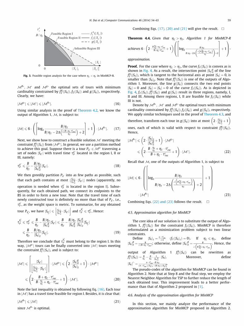
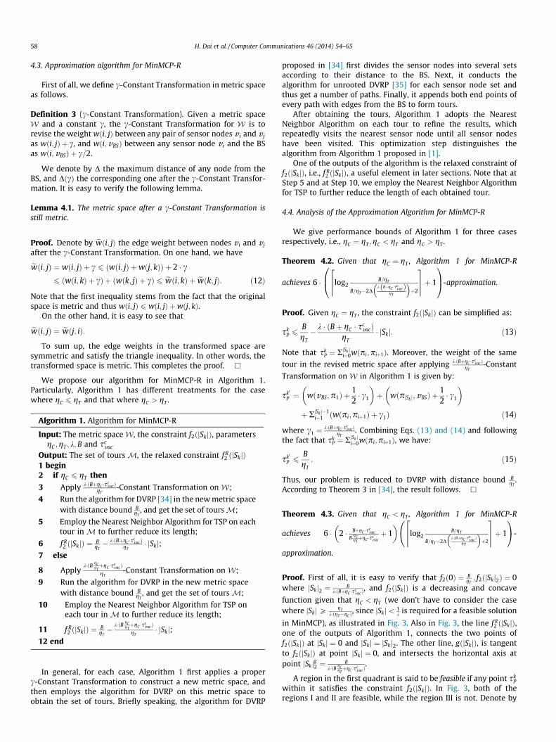
Fig. 3. Feasible region analysis for the case where gC < gT in MinMCP-R.

H. Dai et al. / Computer Communications 46 (2014) 54–65 59

MR�; M� and Mg� the optimal sets of tours with minimumcardinality constrained by f R

2 ðjSkjÞ; f2ðjSkjÞ and gðjSkjÞ, respectively.Clearly, we have:

jMg�j 6 jM�j 6 jMR�j: ð16Þ

Using similar analysis in the proof of Theorem 4.2, we know theoutput of Algorithm 1, M, is subject to:

jMj 6 6 � log2B=gT

B=gT � 2D k�ðBþgC �scvacÞ

gT

� �þ 2

26663777þ 1

0@ 1A � jMR�j: ð17Þ

Next, we show how to construct a feasible solutionM0 meeting theconstraint f R

2 ðjSkjÞ from jMg�j. In general, we use a partition methodto achieve this goal. Suppose there is a tour Pkr 2Mg� traversing aset of nodes jSkr j with travel time skr

P located in the region I, II orIII, namely:

skr

P 6BgT� B=gT

jSkjg2jSkr j: ð18Þ

We then greedily partition Pkr into as few paths as possible, such

that each path contains at most bjSk j2jSk j

g2� jSkr jc nodes (apparently, no

operation is needed when skr

P is located in the region I). Subse-quently, for each obtained path, we connect its endpoints to theBS in order to form a new tour. Note that the travel time of eachnewly constructed tour is definitely no more than that of Pkr , i.e.,skr

P , as the weight space is metric. To summarize, for any obtained

tour Pkrj, we have jSkr

jj 6 jSk j2

jSk jg2� jSkr j

� �and skr

jP 6 skr

P , Hence:

skrj

P 6 skr

P 6BgT� B=gT

jSkjg2jSkr j 6 B

gT� B=gT

jSkjg2jSkjg2jSkj2

jSkrjj

6BgT� B=gT

jSkj2jSkr

jj: ð19Þ

Therefore we conclude that skrj

P must belong to the region I. In thisway, jMg�j tours can be finally converted into jM0j tours meetingthe constraint f R

2 ðjSkjÞ, and is subject to:

jM0j 6 jSkr jjSk j2jSk j

g2� jSkr j

� �266666

377777 � jMg�j 6 2 � jSkjg2

jSkj2þ 1

� �� jMg�j

6 2 � Bþ gC � scvac

B � gCgTþ gC � sc

vac

þ 1

!� jM�j: ð20Þ

Note the last inequality is obtained by following Eq. (16). Each tourin jM0j has a travel time feasible for region I. Besides, it is clear that:

jMR�j 6 jM0j ð21Þ

since MR� is optimal.

Combining Eqs. (17), (20) and (21) will give the result. h

Theorem 4.4. Given that gC > gT , Algorithm 1 for MinMCP-R

achieves 6 � 2 �B�gC

gTþgC �sc

vac

BþgC �scvacþ 1

� �log2

B=gT

B=gT�2Dk� B�

gCgTþgC �s

cvacð Þ

gT

� �þ2

266666377777þ 1

0BB@1CCA-

approximation.

Proof. For the case where gC > gT , the curve f2ðjSkjÞ is convex as isshown in Fig. 4. As a result, the intersection point jSkjg2 of the linef R2 ðjSkjÞ, which is tangent to the horizontal axis at point jSkj ¼ 0, is

smaller than jSkj2. Note that f R2 ðjSkjÞ is one of the outputs of Algo-

rithm 1. Moreover, the line gðjSkjÞ connects the two end pointsjSkj ¼ 0 and jSkj ¼ jSkj ¼ 0 of the curve f2ðjSkjÞ. As is depicted inFig. 4, f2ðjSkjÞ; f R

2 ðjSkjÞ and gðjSkjÞ result in three regions, namely, I,II and III. Among there regions, I, II are feasible for f2ðjSkjÞ whileIII is not.

Denote byMR�; M� andMg� the optimal tours with minimumcardinality constrained by f R

2 ðjSkjÞ; f2ðjSkjÞ and gðjSkjÞ, respectively.We apply similar techniques used in the proof of Theorem 4.3, and

therefore, transform each tour in gðjSkjÞ into at most 2 � jSk j2jSk jg2þ 1

� �ones, each of which is valid with respect to constraint f R

2 ðjSkjÞ.Hence,

jMR�j 6 2 � jSkj2jSkjg2

þ 1� �

� jMg�j

6 2 �B � gC

gTþ gC � sc

vac

Bþ gC � scvac

þ 1

!� jM�j: ð22Þ

Recall that M, one of the outputs of Algorithm 1, is subject to

jMj 6 6 � log2B=gT

B=gT � 2Dk� B�gC

gTþgC �sc

vac

� �gT

0@ 1Aþ 2

2666666666

3777777777þ 1

0BBBBBB@

1CCCCCCA� jMR�j ð23Þ

Combining Eqs. (22) and (23) follows the result. h

4.5. Approximation algorithm for MinMCP

The core idea of our solution is to substitute the output of Algo-rithm 1, f R

2 ðjSkjÞ for the constraint f2ðjSkjÞ. MinMCP is thereforereformulated as a minimization problem subject to two linearconstraints.

Define jSkj1 ¼a�sc

vack�a ðf1ðjSkj1Þ ¼ 0Þ. If gC 6 gT , define

jSkjR2 ¼ Bk�ðBþgC �sc

vacÞ; otherwise, define jSkjR2 ¼ B

k� B�gCgTþgC �sc

vac

� �. Hence, the

output of Algorithm 1 f R2 ðjSkjÞ can be rewritten as

f R2 ðjSkjÞ ¼ B

gT� B

gT� 1jSk jR2� jSkj. Moreover, define

jSkj\ ¼ a�scvac�B=gT

ða�scvacÞ=jSk j1�ðB=gT Þ=jSk jR2

.

The pseudo-codes of the algorithm for MinMCP can be found inAlgorithm 2. Note that at Step 8 and the final step, we employ theNearest Neighbor Algorithm for TSP to further reduce the length ofeach obtained tour. This improvement leads to a better perfor-mance than that of Algorithm 2 proposed in [1].

4.6. Analysis of the approximation algorithm for MinMCP

In this section, we mainly analyze the performance of theapproximation algorithm for MinMCP proposed in Algorithm 2.

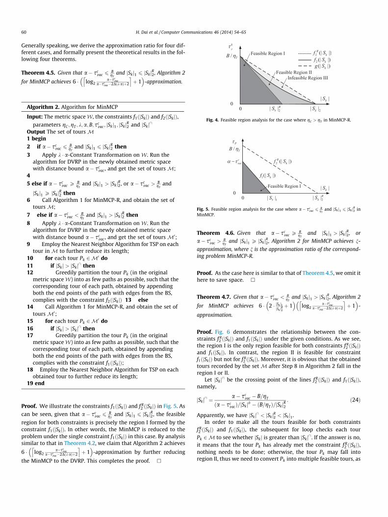
Fig. 4. Feasible region analysis for the case where gC > gT in MinMCP-R.

Fig. 5. Feasible region analysis for the case where a� scvac 6

BgT

and jSkj1 6 jSkjR2 inMinMCP.

60 H. Dai et al. / Computer Communications 46 (2014) 54–65

Generally speaking, we derive the approximation ratio for four dif-ferent cases, and formally present the theoretical results in the fol-lowing four theorems.

Theorem 4.5. Given that a� scvac 6

BgT

and jSkj1 6 jSkjR2, Algorithm 2

for MinMCP achieves 6 � log2a�sc

vaca�sc

vac�2Dðk�aÞþ2

l mþ 1

� �-approximation.

Algorithm 2. Algorithm for MinMCP

Input: The metric spaceW, the constraints f1ðjSkjÞ and f2ðjSkjÞ,parameters gC ;gT ; k;a;B; sc

vac; jSkj1; jSkjR2 and jSkj\

Output The set of tours M1 begin

2 if a� scvac 6

BgT

and jSkj1 6 jSkjR2 then

3 Apply k � a-Constant Transformation on W. Run thealgorithm for DVRP in the newly obtained metric spacewith distance bound a� sc

vac , and get the set of tours M;4

5 else if a� scvac P B

gTand jSkj1 > jSkjR2, or a� sc

vac >BgT

and

jSkj1 P jSkjR2 then6 Call Algorithm 1 for MinMCP-R, and obtain the set of

tours M;

7 else if a� scvac <

BgT

and jSkj1 > jSkjR2 then

8 Apply k � a-Constant Transformation on W. Run thealgorithm for DVRP in the newly obtained metric spacewith distance bound a� sc

vac , and get the set of tours M0;9 Employ the Nearest Neighbor Algorithm for TSP on each

tour in M to further reduce its length;10 for each tour Pk 2M0 do11 if jSkj > jSkj\ then12 Greedily partition the tour Pk (in the original

metric spaceW) into as few paths as possible, such that thecorresponding tour of each path, obtained by appendingboth the end points of the path with edges from the BS,complies with the constraint f2ðjSkjÞ 13 else

14 Call Algorithm 1 for MinMCP-R, and obtain the set oftours M0;

15 for each tour Pk 2M0 do16 if jSkj > jSkj\ then17 Greedily partition the tour Pk (in the original

metric spaceW) into as few paths as possible, such that thecorresponding tour of each path, obtained by appendingboth the end points of the path with edges from the BS,complies with the constraint f1ðjSkjÞ;

18 Employ the Nearest Neighbor Algorithm for TSP on eachobtained tour to further reduce its length;

19 end

Proof. We illustrate the constraints f1ðjSkjÞ and f R2 ðjSkjÞ in Fig. 5. As

can be seen, given that a� scvac 6

BgT

and jSkj1 6 jSkjR2, the feasible

region for both constraints is precisely the region I formed by theconstraint f1ðjSkjÞ. In other words, the MinMCP is reduced to theproblem under the single constraint f1ðjSkjÞ in this case. By analysissimilar to that in Theorem 4.2, we claim that Algorithm 2 achieves

6 � log2a�sc

vaca�sc

vac�2Dðk�aÞþ2

l mþ 1

� �-approximation by further reducing

the MinMCP to the DVRP. This completes the proof. h

Theorem 4.6. Given that a� scvac P B

gTand jSkj1 > jSkjR2, or

a� scvac >

BgT

and jSkj1 P jSkjR2, Algorithm 2 for MinMCP achieves n-

approximation, where n is the approximation ratio of the correspond-ing problem MinMCP-R.

Proof. As the case here is similar to that of Theorem 4.5, we omit ithere to save space. h

Theorem 4.7. Given that a� scvac <

BgT

and jSkj1 > jSkjR2, Algorithm 2

for MinMCP achieves 6 � 2 � jSk j1jSk jR2þ 1

� �log2

a�scvac

a�scvac�2Dðk�aÞþ2

l mþ 1

� �-

approximation.

Proof. Fig. 6 demonstrates the relationship between the con-straints f R

2 ðjSkjÞ and f1ðjSkjÞ under the given conditions. As we see,the region I is the only region feasible for both constraints f R

2 ðjSkjÞand f1ðjSkjÞ. In contrast, the region II is feasible for constraintf1ðjSkjÞ but not for f R

2 ðjSkjÞ. Moreover, it is obvious that the obtainedtours recorded by the setM after Step 8 in Algorithm 2 fall in theregion I or II.

Let jSkj\ be the crossing point of the lines f R2 ðjSkjÞ and f1ðjSkjÞ,

namely,

jSkj\ ¼a� sc

vac � B=gT

ða� scvacÞ=jSkj/ � ðB=gTÞ=jSkjR2

: ð24Þ

Apparently, we have jSkj\ < jSkjR2 < jSkj1.In order to make all the tours feasible for both constraints

f R2 ðjSkjÞ and f1ðjSkjÞ, the subsequent for loop checks each tour

Pk 2M to see whether jSkj is greater than jSkj\. If the answer is no,it means that the tour Pk has already met the constraint f R

2 ðjSkjÞ,nothing needs to be done; otherwise, the tour Pk may fall intoregion II, thus we need to convert Pk into multiple feasible tours, as

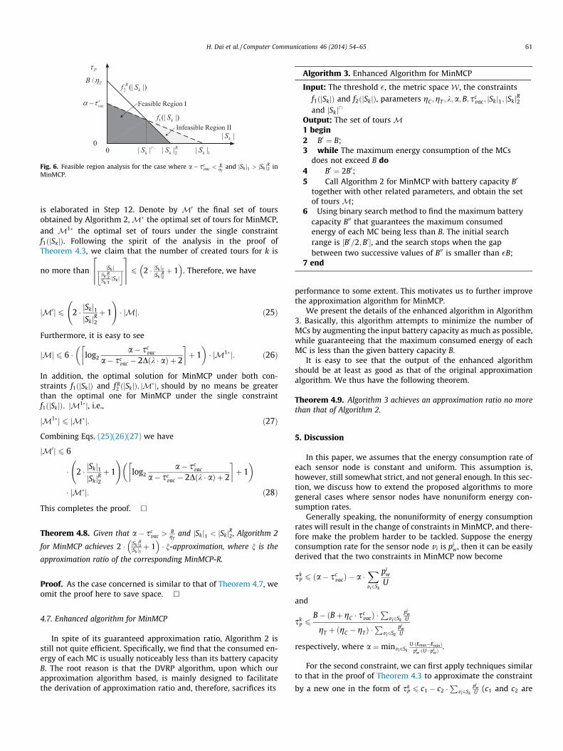
Fig. 6. Feasible region analysis for the case where a� scvac <

BgT

and jSkj1 > jSkjR2 inMinMCP.

H. Dai et al. / Computer Communications 46 (2014) 54–65 61

is elaborated in Step 12. Denote by M0 the final set of toursobtained by Algorithm 2,M� the optimal set of tours for MinMCP,and M1� the optimal set of tours under the single constraintf1ðjSxjÞ. Following the spirit of the analysis in the proof ofTheorem 4.3, we claim that the number of created tours for k is

no more than jSk jjSk j

R2

jSk j1�jSk j

j k26663777 6 2 � jSk j1

jSk jR2þ 1

� �. Therefore, we have

jM0j 6 2 � jSkj1jSkjR2

þ 1

!� jMj: ð25Þ

Furthermore, it is easy to see

jMj 6 6 � log2a� sc

vac

a� scvac � 2Dðk � aÞ þ 2

� þ 1

� �� jM1�j: ð26Þ

In addition, the optimal solution for MinMCP under both con-straints f1ðjSkjÞ and f R

2 ðjSkjÞ; jM�j, should by no means be greaterthan the optimal one for MinMCP under the single constraintf1ðjSkjÞ; jM1�j, i.e.,

jM1�j 6 jM�j: ð27Þ

Combining Eqs. (25)(26)(27) we have

jM0j 6 6

� 2 � jSkj1jSkjR2

þ 1

!log2

a� scvac

a� scvac � 2Dðk � aÞ þ 2

� þ 1

� �� jM�j: ð28Þ

This completes the proof. h

Theorem 4.8. Given that a� scvac >

BgT

and jSkj1 < jSkjR2, Algorithm 2

for MinMCP achieves 2 � jSk jR2jSk j1þ 1

� �� n-approximation, where n is the

approximation ratio of the corresponding MinMCP-R.

Proof. As the case concerned is similar to that of Theorem 4.7, weomit the proof here to save space. h

4.7. Enhanced algorithm for MinMCP

In spite of its guaranteed approximation ratio, Algorithm 2 isstill not quite efficient. Specifically, we find that the consumed en-ergy of each MC is usually noticeably less than its battery capacityB. The root reason is that the DVRP algorithm, upon which ourapproximation algorithm based, is mainly designed to facilitatethe derivation of approximation ratio and, therefore, sacrifices its

Algorithm 3. Enhanced Algorithm for MinMCP

Input: The threshold �, the metric space W, the constraints

f1ðjSkjÞ and f2ðjSkjÞ, parameters gC ;gT ; k;a;B; scvac; jSkj1; jSkjR2

and jSkj\Output: The set of tours M1 begin2 B0 ¼ B;3 while The maximum energy consumption of the MCs

does not exceed B do4 B0 ¼ 2B0;5 Call Algorithm 2 for MinMCP with battery capacity B0

together with other related parameters, and obtain the setof tours M;

6 Using binary search method to find the maximum batterycapacity B00 that guarantees the maximum consumedenergy of each MC being less than B. The initial searchrange is ½B0=2;B0�, and the search stops when the gapbetween two successive values of B00 is smaller than �B;

7 end

performance to some extent. This motivates us to further improvethe approximation algorithm for MinMCP.

We present the details of the enhanced algorithm in Algorithm3. Basically, this algorithm attempts to minimize the number ofMCs by augmenting the input battery capacity as much as possible,while guaranteeing that the maximum consumed energy of eachMC is less than the given battery capacity B.

It is easy to see that the output of the enhanced algorithmshould be at least as good as that of the original approximationalgorithm. We thus have the following theorem.

Theorem 4.9. Algorithm 3 achieves an approximation ratio no morethan that of Algorithm 2.

5. Discussion

In this paper, we assumes that the energy consumption rate ofeach sensor node is constant and uniform. This assumption is,however, still somewhat strict, and not general enough. In this sec-tion, we discuss how to extend the proposed algorithms to moregeneral cases where sensor nodes have nonuniform energy con-sumption rates.

Generally speaking, the nonuniformity of energy consumptionrates will result in the change of constraints in MinMCP, and there-fore make the problem harder to be tackled. Suppose the energyconsumption rate for the sensor node v i is pi

w, then it can be easilyderived that the two constraints in MinMCP now become

skP 6 ða� sc

vacÞ � a �Xv i2Sk

piw

U

and

skP 6

B� ðBþ gC � scvacÞ �

Pv i2Sk

piw

U

gT þ ðgC � gTÞ �P

v i2Sk

piw

U

respectively, where a ¼minv i2Sk

U�ðEmax�EminÞpi

w �ðU�piwÞ

.

For the second constraint, we can first apply techniques similarto that in the proof of Theorem 4.3 to approximate the constraint

by a new one in the form of skP 6 c1 � c2 �

Pv i2Sk

piw

U (c1 and c2 are

1 2 3 4 5 6 7 8 90

2

4

6

8

Mobile Charger ID

Num

ber o

f Rec

harg

ed N

odes

1 2 3 4 5 6 7 8 90

2000

4000

6000

8000

Mobile Charger ID

Trav

el D

ista

nce

(m)

1 2 3 4 5 6 7 8 90

0.5

1

1.5

2x 105

Mobile Charger ID

Ener

gy C

onsu

mpt

ion

(J)

1 2 3 4 5 6 7 8 90

2000

4000

6000

8000

Mobile Charger ID

Rec

harg

e Pe

riod

τk (S)

Fig. 9. Critical parameters of each MC when B ¼ 180 KJ.

0 1000 2000 3000 4000 5000

0

1000

2000

3000

4000

5000

BS

X (m)

Y (m

)

Fig. 7. An instance to the enhanced approximation algorithm for MinMCP whenB ¼ 300 KJ.

0 1000 2000 3000 4000 5000

0

1000

2000

3000

4000

5000

BS

X (m)

Y (m

)

Fig. 8. An instance to the enhanced approximation algorithm for MinMCP whenB ¼ 180 KJ.

62 H. Dai et al. / Computer Communications 46 (2014) 54–65

positive constants), then employ an extended transformation tech-nique based on c-Constant Transformation to further convert theconstraint to the form of sk

P 6 c3, where c3 is a constant. The origi-nal constraint is thus transformed to the traditional constraint ofDVRP.

On the contrary, the first constraint is harder to be treated. Thisis because a is not a constant but a variable relating to the energyconsumption rates of the nodes contained in the visiting set of sen-sor nodes Sk of the MC k. In the future work, we will devise newapproximation approaches to deal with this problem, as well asthe original problem when considering both of the constraints.

6. Simulation results

In this section, we present simulation results to verify our the-oretical findings. We first introduce the evaluation setup, followedby the description of the baseline algorithm. Next, we illustrate aninstance of the enhanced MinMCP algorithm, and then evaluate theperformance of the proposed algorithms in terms of the batterycapacity B; Emax � Emin for sensor nodes, energy transfer rate U,charging power for MCs gC and number of sensor nodes. For theevaluation regarding these parameters, every point on the plottedfigures stands for the average value over that of 100 randomly gen-erated topologies.

6.1. Evaluation Setup

We randomly distribute 50 sensor nodes in a 5 km� 5 km 2DEuclidian region throughout the simulations. Any pair of nodes canreach each other through a direct path. The base station is assumedto be located at ð2500 m;2500 mÞ. Unless otherwise specified, weuse the following parameter settings as in [14]: the traveling speedof MCs is V ¼ 5 m=s; pw ¼ 200 mW; Emax ¼ 10:8 kJ; Emin ¼ 540 J;U ¼ 5 W;gC ¼ 110 W;gT ¼ 100 W;B ¼ 500 KJ and sc

vac ¼ 1 hour.

6.2. Baseline setup

Though the algorithm proposed in [22] is related to our work, itis not appropriate to use it directly for comparison. On the onehand, it is only suitable for 1D sensor networks. On the other hand,it adopts a different assumption, namely, MCs can intentionallygather at a rendezvous point to recharge others or to be rechargedwithout energy loss. This assumption finally leads to a completelydifferent scheme compared with ours. For this reason, we con-struct the following baseline algorithm by borrowing ideas of[22] for comparison. That is, all the MCs dictated by this algorithmhave uniform schedule periods, which means that the MCs that fin-ish the charging tasks earlier have to wait at BS for the returns ofother MCs before starting the next trip. The chargers plan theirroutes in sequence. For each charger, it consistently chooses thenearest sensor node that is not chosen by the former chargers tocharge after its departure from the BS. At each step, the chargerchecks whether its residual energy can sustain its next move tothe next node and returning back to the BS. If not, the charger goesback to the BS immediately. The length of the schedule period ofeach charger is set to be the average length of the schedule periodsdetermined by our algorithm for MinMCP, such that the renewableenergy cycle of each sensor node can be guaranteed.

6.3. Performance evaluation

6.3.1. An Instance to the enhanced approximation algorithm forMinMCP

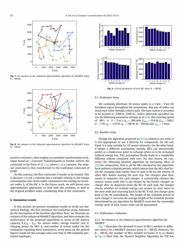
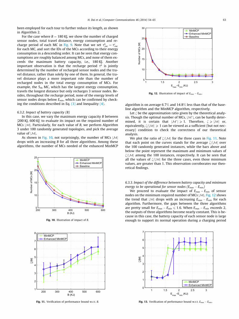
Fig. 7 illustrates the obtained 4 tours of MCs (marked in differ-ent colors) for a MinMCP instance given B ¼ 300 KJ. However, forB ¼ 180 KJ, the number of MCs needed increases to 9, as shownin Fig. 8. Note that, the Nearest Neighbor Algorithm for TSP has

1 1.5 2 2.5 35

10

15

20

25

30

Emax−Emin (KJ)

Num

ber o

f MC

s |M

|

MinMCPEnhanced MinMCPBaseline

Fig. 12. Illustration of impact of Emax � Emin .

H. Dai et al. / Computer Communications 46 (2014) 54–65 63

been employed for each tour to further reduce its length, as shownin Algorithm 2.

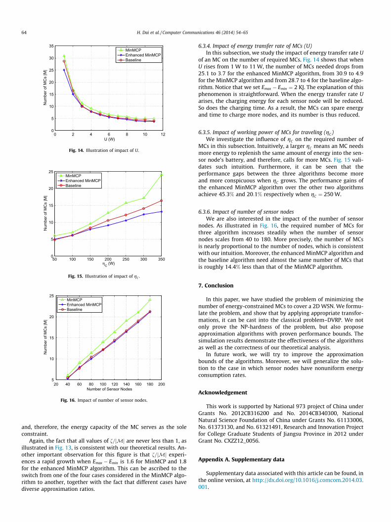
For the case where B ¼ 180 KJ, we show the number of chargedsensor nodes, total travel distance, energy consumption and re-charge period of each MC in Fig. 9. Note that we set sk

vac ¼ scvac

for each MC, and sort the IDs of the MCs according to their energyconsumption in a descending order. It can be seen that energy con-sumptions are roughly balanced among MCs, and none of them ex-ceeds the maximum battery capacity, i.e., 180 KJ. Anotherimportant observation is that the recharge period sk is jointlydetermined by the number of recharged sensor nodes and the tra-vel distance, rather than solely by one of them. In general, the tra-vel distance plays a more important role than the number ofrecharged nodes in the total energy consumption of MCs. Forexample, the 5th MC, which has the largest energy consumption,travels the longest distance but only recharges 3 sensor nodes. Be-sides, throughout the recharge period, none of the energy levels ofsensor nodes drops below Emin, which can be confirmed by check-ing the conditions described in Eq. (3) and Inequality (4).

6.3.2. Impact of battery capacity (B)In this case, we vary the maximum energy capacity B between

½200 KJ, 600 KJ� to evaluate its impact on the required number ofMCs jMj. Particularly, for each value of B, we perform Algorithm3 under 100 randomly generated topologies, and pick the averagevalue of jMj.

As shown in Fig. 10, not surprisingly, the number of MCs jMjdrops with an increasing B for all three algorithms. Among thesealgorithms, the number of MCs needed of the enhanced MinMCP

200 300 400 500 6001

2

3

4

5

6

7

8

B (KJ)

ζ/|M

|

MinMCPEnhanced MinMCP

Fig. 11. Verification of performance bound w.r.t. B.

200 300 400 500 6005

10

15

20

25

B (KJ)

Num

ber o

f MC

s |M

|

MinMCPEnhanced MinMCPBaseline

Fig. 10. Illustration of impact of B.

algorithm is on average 6:7% and 14:8% less than that of the base-line algorithm and the MinMCP algorithm, respectively.

Let f be the approximation ratio given by the theoretical analy-sis. Though the optimal number of MCs, jM�j, can be hardly deter-mined, it is certain that jM�jP 1. Therefore, f P jMj or,equivalently, f=jMjP 1 can be viewed as a sufficient (but not nec-essary) condition to check the correctness of our theoreticalanalysis.

We plot the ratio of f=jMj for the three cases in Fig. 11. Notethat each point on the curves stands for the average f=jMj overthe 100 randomly generated instances, while the bars above andbelow the point represent the maximum and minimum values off=jMj among the 100 instances, respectively. It can be seen thatall the values of f=jMj for the three cases, even those minimumvalues, are greater than 1. This observation corroborates our theo-retical findings.

6.3.3. Impact of the difference between battery capacity and minimumenergy to be operational for sensor nodes (Emax � Emin)

We proceed to evaluate the impact of Emax � Emin of sensornodes on the minimum required number of MCs jMj. Fig. 12 showsthe trend that jMj drops with an increasing Emax � Emin for eachalgorithm. Furthermore, the gaps between the three algorithmsare pretty small for Emax � Emin 6 1:6. When Emax � Emin exceeds 2,the outputs of three algorithms become nearly constant. This is be-cause in this case, the battery capacity of each sensor node is largeenough to support its normal operation during a charging period

1 1.5 2 2.5 30

1

2

3

4

5

6

7

Emax−Emin (KJ)

ζ/|M

|

MinMCPEnhanced MinMCP

Fig. 13. Verification of performance bound w.r.t. Emax � Emin .

0 2 4 6 8 10 120

5

10

15

20

25

30

35

U (W)

Num

ber o

f MC

s |M

|MinMCPEnhanced MinMCPBaseline

Fig. 14. Illustration of impact of U.

50 100 150 200 250 300 3500

5

10

15

20

25

ηC (W)

Num

ber o

f MC

s |M

|

MinMCPEnhanced MinMCPBaseline

Fig. 15. Illustration of impact of gC .

20 40 60 80 100 120 140 160 180 2005

10

15

20

25

Number of Sensor Nodes

Num

ber o

f MC

s |M

|

MinMCPEnhanced MinMCPBaseline

Fig. 16. Impact of number of sensor nodes.

64 H. Dai et al. / Computer Communications 46 (2014) 54–65

and, therefore, the energy capacity of the MC serves as the soleconstraint.

Again, the fact that all values of f=jMj are never less than 1, asillustrated in Fig. 13, is consistent with our theoretical results. An-other important observation for this figure is that f=jMj experi-ences a rapid growth when Emax � Emin is 1.6 for MinMCP and 1.8for the enhanced MinMCP algorithm. This can be ascribed to theswitch from one of the four cases considered in the MinMCP algo-rithm to another, together with the fact that different cases havediverse approximation ratios.

6.3.4. Impact of energy transfer rate of MCs (U)In this subsection, we study the impact of energy transfer rate U

of an MC on the number of required MCs. Fig. 14 shows that whenU rises from 1 W to 11 W, the number of MCs needed drops from25:1 to 3:7 for the enhanced MinMCP algorithm, from 30:9 to 4:9for the MinMCP algorithm and from 28:7 to 4 for the baseline algo-rithm. Notice that we set Emax � Emin ¼ 2 KJ. The explanation of thisphenomenon is straightforward. When the energy transfer rate Uarises, the charging energy for each sensor node will be reduced.So does the charging time. As a result, the MCs can spare energyand time to charge more nodes, and its number is thus reduced.

6.3.5. Impact of working power of MCs for traveling (gC)We investigate the influence of gC on the required number of

MCs in this subsection. Intuitively, a larger gC means an MC needsmore energy to replenish the same amount of energy into the sen-sor node’s battery, and therefore, calls for more MCs. Fig. 15 vali-dates such intuition. Furthermore, it can be seen that theperformance gaps between the three algorithms become moreand more conspicuous when gC grows. The performance gains ofthe enhanced MinMCP algorithm over the other two algorithmsachieve 45:3% and 20:1% respectively when gC ¼ 250 W.

6.3.6. Impact of number of sensor nodesWe are also interested in the impact of the number of sensor

nodes. As illustrated in Fig. 16, the required number of MCs forthree algorithm increases steadily when the number of sensornodes scales from 40 to 180. More precisely, the number of MCsis nearly proportional to the number of nodes, which is consistentwith our intuition. Moreover, the enhanced MinMCP algorithm andthe baseline algorithm need almost the same number of MCs thatis roughly 14:4% less than that of the MinMCP algorithm.

7. Conclusion

In this paper, we have studied the problem of minimizing thenumber of energy-constrained MCs to cover a 2D WSN. We formu-late the problem, and show that by applying appropriate transfor-mations, it can be cast into the classical problem–DVRP. We notonly prove the NP-hardness of the problem, but also proposeapproximation algorithms with proven performance bounds. Thesimulation results demonstrate the effectiveness of the algorithmsas well as the correctness of our theoretical analysis.

In future work, we will try to improve the approximationbounds of the algorithms. Moreover, we will generalize the solu-tion to the case in which sensor nodes have nonuniform energyconsumption rates.

Acknowledgement

This work is supported by National 973 project of China underGrants No. 2012CB316200 and No. 2014CB340300, NationalNatural Science Foundation of China under Grants No. 61133006,No. 61373130, and No. 61321491, Research and Innovation Projectfor College Graduate Students of Jiangsu Province in 2012 underGrant No. CXZZ12_0056.

Appendix A. Supplementary data

Supplementary data associated with this article can be found, inthe online version, at http://dx.doi.org/10.1016/j.comcom.2014.03.001.

H. Dai et al. / Computer Communications 46 (2014) 54–65 65

References

[1] H. Dai, X. Wu, L. Xu, G. Chen, S. Lin, Using minimum mobile chargers to keeplarge-scale wireless rechargeable sensor networks running forever, in: ICCCN,2013.

[2] V. Raghunathan, A. Kansal, J. Hsu, J. Friedman, M. Srivastava, Designconsiderations for solar energy harvesting wireless embedded systems, in:Proceedings of the 4th International Symposium on Information Processing inSensor Networks, IEEE Press, 2005, p. 64.

[3] S. Meninger, J. Mur-Miranda, R. Amirtharajah, A. Chandrakasan, J. Lang,Vibration-to-electric energy conversion, IEEE Transactions on Very Large ScaleIntegration (VLSI) Systems 9 (1) (2001) 64–76.

[4] C. Park, P. Chou, Ambimax: autonomous energy harvesting platform for multi-supply wireless sensor nodes, in: SECON, 2006.

[5] A. Kurs, A. Karalis, M. Robert, J.D. Joannopoulos, P. Fisher, M. Soljacic, Wirelesspower transfer via strongly coupled magnetic resonances, Science 317 (5834)(2007) 83–86.

[6] <http://www.seattle.intel-research.net/wisp/>.[7] H. Dai, Y. Liu, G. Chen, X. Wu, T. He, Safe charging for wireless power transfer,

in: INFOCOM, 2014.[8] <http://www.powermat.com>.[9] <http://www.laptopmag.com/reviews/laptops/dell-latitude-3330.aspx>.

[10] <http://evworld.com/news.cfm?newsid=24420>.[11] M. Erol-Kantarci, H. Mouftah, Suresense: sustainable wireless rechargeable

sensor networks for the smart grid, Wireless Commun., IEEE 19 (3) (2012) 30–36.[12] D. Mascareñas, E. Flynn, M. Todd, G. Park, C. Farrar, Wireless sensor

technologies for monitoring civil structures, Sound Vibr. 42 (4) (2008) 16–21.[13] B. Tong, Z. Li, G. Wang, W. Zhang, How wireless power charging technology

affects sensor network deployment and routing, in: ICDCS, 2010.[14] Y. Shi, L. Xie, Y.T. Hou, H.D. Sherali, On renewable sensor networks with

wireless energy transfer, in: INFOCOM, 2011.[15] Z. Li, Y. Peng, W. Zhang, D. Qiao, J-RoC: a joint routing and charging scheme to

prolong sensor network lifetime, in: IPSN, 2011.[16] K. Li, H. Luan, C. Shen, Qi-ferry: energy-constrained wireless charging in

wireless sensor networks, in: WCNC, 2012.[17] C. Farrar, G. Park, M. Todd, Sensing network paradigms for structural health

monitoring, New Dev. Sensing Technol. Struct. Health Monitor. (2011) 137–157.

[18] H. Dai, L. Jiang, X. Wu, D.K. Yau, G. Chen, S. Tang, Near optimal charging andscheduling scheme for stochastic event capture with rechargeable sensors, in:MASS, 2013.

[19] S. He, J. Chen, F. Jiang, D.K.Y. Yau, G. Xing, Y. Sun, Energy provisioning inwireless rechargeable sensor networks, in: INFOCOM, 2011.

[20] H. Dai, X. Wu, L. Xu, G. Chen, Practical scheduling for stochastic event capturein wireless rechargeable sensor networks, in: WCNC, 2013.

[21] H. Dai, L. Xu, X. Wu, C. Dong, G. Chen, Impact of mobility on energyprovisioning in wireless rechargeable sensor networks, in: WCNC, 2013.

[22] S. Zhang, J. Wu, S. Lu, Collaborative mobile charging for sensor networks, in:MASS, 2012.

[23] M. Zhao, J. Li, Y. Yang, Joint mobile energy replenishment and data gathering inwireless rechargeable sensor networks, in: ITC, 2011.

[24] S. Guo, C. Wang, Y. Yang, Mobile data gathering with wireless energyreplenishment in rechargeable sensor networks, in: INFOCOM, 2013.

[25] L. Xie, Y. Shi, Y.T. Hou, W. Lou, H.D. Sherali, S.F. Midkiff, Bundling mobile basestation and wireless energy transfer: Modeling and optimization, Tech. rep.,2013.

[26] L. Fu, P. Cheng, Y. Gu, J. Chen, T. He, Minimizing charging delay in wirelessrechargeable sensor networks, in: INFOCOM, 2013.

[27] L. He, Y. Gu, J. Pan, T. Zhu, On-demand charging in wireless sensor networks:theories and applications, in: MASS, 2013.

[28] O. Jonah, S. Georgakopoulos, Wireless power transmission to sensorsembedded in concrete via magnetic resonance, in: WAMICON, 2011.

[29] J.M. Engel, L. Zhao, Z. Fan, J. Chen, C. Liu, Smart brick-a low cost, modularwireless sensor for civil structure monitoring, in: CCCT, 2004.

[30] S.G. Taylor, K.M. Farinholt, E.B. Flynn, E. Figueiredo, D.L. Mascarenas, E.A. Moro,G. Park, M.D. Todd, C.R. Farrar, A mobile-agent-based wireless sensing networkfor structural monitoring applications, Measure. Sci. Technol. 20 (4) (2009)045201.

[31] M. Buettner, R. Prasad, M. Philipose, D. Wetherall, Recognizing daily activitieswith rfid-based sensors, in: Ubicomp, 2009.

[32] M. Buettner, B. Greenstein, A. Sample, J. Smith, D. Wetherall, Revisiting smartdust with rfid sensor networks, in: Proceedings of the 7th ACM Workshop onHot Topics in Networks, 2008.

[33] F. Jiang, S. He, P. Cheng, J. Chen, On optimal scheduling in wirelessrechargeable sensor networks for stochastic event capture, in: MASS, 2011.

[34] V. Nagarajan, R. Ravi, Approximation algorithms for distance constrainedvehicle routing problems, Networks 59 (2) (2012) 209–214.

[35] E.M. Arkin, R. Hassin, A. Levin, Approximations for minimum and min–maxvehicle routing problems, J. Algorithms 59 (1) (2006) 1–18.