Embed Size (px)
Citation preview
Operations Research Letters 25 (1999) 219–230www.elsevier.com/locate/orms
Minimax regret strategies for greenhouse gas abatement:methodology and application(
Richard Loulou ∗, Amit KanudiaGERAD, Ecole des Hautes Etudes Commerciales, 3000, Ch. de la Cote-Ste-Catherine, Montreal, QC, Canada H3T 2A7
Received 1 March 1998; received in revised form 1 April 1999
Abstract
Classical stochastic programming has already been used with large-scale LP models for long-term analysis of energy–environment systems. We propose a Minimax Regret formulation suitable for large-scale linear programming models. Ithas been experimentally veri�ed that the minimax regret strategy depends only on the extremal scenarios and not on theintermediate ones, thus making the approach computationally e�cient. Key results of minimax regret and minimum expectedvalue strategies for Greenhouse Gas abatement in the Province of Qu�ebec, are compared. c© 1999 Elsevier Science B.V.All rights reserved.
Keywords: Energy; Environment; Stochastic programming; Minimax regret
1. Introduction
The Global Warming of the terrestrial atmosphereinduced by an increase inGreenhouseGas (GHG) con-centration has moved from speculation to fact in therecent years. A major set of studies by the Intergovern-mental Panel on Climate Change [8–10,14] summa-rizes research in these areas over more than a decade.In spite of the recent Kyoto Protocol establishing
abatement targets to be achieved by 2010 in industri-alized countries, there still remain large uncertainties,both on the e�ective attainment of these targets, and
( Research supported by Natural Science and Engineering Re-search Council of Canada, FCAR (Qu�ebec), Environment Canada,and Shastri Indo-Canadian Institute.
∗ Corresponding author.E-mail addresses: [email protected] (R. Loulou),
[email protected] (A. Kanudia)
on additional reduction levels beyond 2010. The Ky-oto Protocol, as well as debates in forums like theIPCC, give some indication of the range in whichthe long-term abatement targets can lie. In a nutshell,the basic problem facing policy makers is to decideupon the levels and timing of emission abatement,climate adaptation and geo-engineering responses toclimate change. This directly a�ects short-term energysector investment decisions, because of the long leadtimes and even longer life times of projects in electric-ity generation and transmission, oil re�ning and natu-ral gas supply. In this paper, we focus on the abatementaspects, which are strongly related to a detailed under-standing of the energy system of each country. Specif-ically, we demonstrate the important impacts thatuncertainty may have on policy making, and proposea decision-making paradigm that sheds light on thisimportant issue, namely the Minimax Regret criterion.
0167-6377/99/$ - see front matter c© 1999 Elsevier Science B.V. All rights reserved.PII: S 0167 -6377(99)00049 -8
220 R. Loulou, A. Kanudia /Operations Research Letters 25 (1999) 219–230
The basic question we address in this paper is: howcan we determine an interim energy sector strategy,i.e., before the level and timing of abatement areknown with certainty? The endeavor is to determine astrategy that hedges against all possible requirementsto reduce the GHG emissions by various amounts. Al-though we model the uncertainty in terms of di�erentemission constraints in our model, a similar approachwould be equally relevant for a GHG tax situation.In contrast with the more classical analysis of
decision making under risk, where stochastic pro-gramming is applied to a set of scenarios, each witha probability of occurrence, we propose for this re-search the Minimax Regret criterion to determinethe hedging strategy under uncertainty. This criteriononly needs the list of possible scenarios, without anyassumption on their probabilities. In Section 2, wedescribe the formulation of the minimax regret strat-egy as a linear program. The base model, ExtendedMARKAL, as well as its Stochastic Programming andMinimax Regret variants, are described in Section 3.Section 4 contains the analysis of results.
2. Minimax Regret Formulation of a GHGAbatement Model
2.1. A brief reminder of the Minimax Regretcriterion
The Minimax Regret criterion, also known asSavage criterion, Rai�a [21,22], is one of the morecredible criteria for selecting decisions under uncer-tainty, i.e. when the likelihoods of the various possi-ble outcomes are not known with su�cient precisionto use the classical expected value or expected utilitycriteria. In order to �x ideas, we shall assume in whatfollows that a certain decision problem is couched interms of a cost to minimize (a symmetric formula-tion is obtained in the case of a payo� to maximize).Therefore, we may denote by C(z; s) the cost incurredwhen strategy s is used, and outcome z occurs. TheRegret R(z; s) is de�ned as the di�erence between thecost incurred with the pair (z; s) and the least costachievable under outcome perfect information on z,i.e.:
R(z; s) = C(z; s)−Mint∈S
C(z; t); ∀z ∈ Z; s ∈ S;
where Z is the set of possible outcomes and S is theset of feasible strategies. Note that, by construction, aregret R(z; s) is always non-negative.AMinimax Regret (MMR) strategy is any s∗ that
minimizes the worst regret, i.e.
s∗ ∈ ArgMins∈S
{Maxz∈Z
R(z; s)}
and the corresponding Minimax Regret is equal to
MMR=Mins∈S
{Maxz∈Z
R(z; s)}:
2.2. Minimax Regret for large-scale LinearPrograms
We now turn to the application of the above def-inition to the case when the cost C(z; s) is not anexplicit expression. Rather, it is implicitly computedvia an optimization program. This is the case in par-ticular when using a model such as MARKAL, Fish-bone and Abilock [5], Berger et al. [1], Loulou andLavigne [16], where the long-term energy systemleast cost is computed by solving a large-scale lin-ear program with many technical and economicconstraints, as well as environmental emission con-straints. MARKAL is a nine period dynamic LinearProgram, where each period represents �ve years. Informulation (1) below, the A matrix de�nes the verylarge number of techno-economic constraints of themodel, and the last constraint represents the single cu-mulative greenhouse gas (GHG) emission constraint,i.e. an upper bound on the sum of all emissions overthe model’s 45 year horizon (the choice of a cumula-tive emission constraint will be justi�ed in Section 3).In the absence of uncertainty, the MARKAL linearprogram has the following structure:
M (z) =Minxctx
s:t: Ax6b;
etx6z;
(1)
where x is the vector of MARKAL decision variables(strategy), and z is the selected cumulative emissiontarget.The more interesting and more realistic case oc-
curs when the allowed cumulative emission z is uncer-tain, and will only be known at some future period t∗.

R. Loulou, A. Kanudia /Operations Research Letters 25 (1999) 219–230 221
Prior to t∗, all decisions are taken under uncertainty,whereas at t∗ and later, decisions are taken under per-fect knowledge of the cumulative target. It is conve-nient to decompose the vector x of decision variablesinto two vectors x1 and x2; x1 representing the deci-sions to be taken prior to t∗, and x2 those decisionsat t∗ and later. We shall assume that the uncertainparameter z may take an arbitrary but �nite numbern of distinct values:
Z = {z1; z2; : : : ; zn; z16z26 · · ·6zn}:The linear program in (1), which de�nes an idealcost M (z) that would be incurred under perfect infor-mation, allows to de�ne the Regret of strategy x asfollows:
R(x) = ctx −M (z):Finally, the MMR strategy is an optimal solution tothe following optimization program:
MMR=Minx1 ;x2
Maxz∈Z
[ct1x1 + ct2xz2 −M (z)]
s:t: A1x1 + A2xz2¿b; ∀z ∈ Z;et1x1 + e
t2xz26z; ∀z ∈ Z:
(2)
The above program is not quite an L.P., but may beconverted into one by introducing a new variable:
MMR= Minx1 ;x2 ;�
[�]
s:t: �¿ct1x1 + ct2xz2 −M (z); ∀z ∈ Z;
A1x1 + A2xz2¿b; ∀z ∈ Z;et1x1 + e
t2xz26z; ∀z ∈ Z:
(3)
Note carefully that a bona�de strategy x is such thatx1 is common to all outcomes z, whereas there is adi�erent vector xz2 for each outcome z in Z . This isso because decisions made at t∗ and later take intoaccount the knowledge of the true value of z thatrealizes at t∗. Hence, the LP (3) has up to n rep-lications of the constraints, and of the x2 variables(to be more precise, some constraints which do notinvolve x2 variables are not replicated, and therefore,the size of (3) may be smaller than n times the sizeof (1)).Important remark: An unfortunate phenomenon
occurs when (3) is solved: since all that matters whencomputing the MMR strategy is indeed the value ofthe Minimax Regret, all other regrets are left free to
take any values, as long as these values remain belowthe MMR. This remark is equivalent to saying that(3) is highly degenerate. For example, in the instanceto be discussed later, theMMR is equal to 3311 M$,but when (3) is solved, each of the n regrets (i.e. eachright-hand-side of the �rst constraints of (3)), is foundto be also equal to 3311 M$. This is undesirable, as inpractice, depending upon the actual value of z whichrealizes, the regret can be quite much lower thanMMR. In order to remove the dual degeneracy, it isuseful to proceed in two phases: �rst, consider (3) asessentially only a way of computing the partial strat-egy up to the resolution date, i.e. x1. Next, when thisis done, each xz2 may be computed independently by(i) �xing x1 at its optimal value (call it x∗1 ), and (ii)for each z, solving the following n linear programs:
Minx2
[ct1x∗1 + c
t2x2 −M (z)]
s:t: A1x∗1 + A2x2¿b;
et1x∗1 + e
t2x26z:
(4)
2.3. Computational considerations and a conjecture
The largest LP to solve is clearly (3), which has thesame approximate size as a classical stochastic LP de-�ned on the same problem instance, and using the min-imum expected value criterion (MEV). In addition,n−1 smaller problems (4) must be solved, in order tocompute the n−1 non-degenerate strategies after datet∗. However, it appears from computational experi-ence (and from intuitive reasoning), that the solutionof (3) seems to depend only on a restricted problem.This observation is only a conjecture, which we nowpresent, but were unable to prove in any generality.
Conjecture. When solving problem (2) or (3), it issu�cient to restrict the parameter z to its largest andsmallest values z1 and zn.
This conjecture was veri�ed in all experiments. Iftrue, it considerably reduces the size of the L.P. (3).The maximum size of (3) is approximately twice thatof a deterministic problem such as (1), meaning thatthe number of variables and the number of constraintsare both about double those of (1). This has interestingimplications in terms of the ease of solving the MMR
222 R. Loulou, A. Kanudia /Operations Research Letters 25 (1999) 219–230
problem, which thus becomes easier to solve than aclassical stochastic LP with more than two outcomes.
3. Large-scale application to energy–environmentanalysis
3.1. Uncertainty in energy–environment modeling
Many applications of analysis under risk exist us-ing activity analysis models. We restrict our briefreview to recent energy–environment models. A com-prehensive description and application of a two-stepapproach for evaluating an apriori set of hedging en-ergy technologies can be found in Larsson and Wene[15], and Wene [23]. Their method provided for as-sessing the e�ciency and robustness of exogenouslydetermined alternative strategies, by a two-step use ofthe MARKAL model. Although they did not fully im-plement the Stochastic Programming paradigm, theirwork was the initial inspiration to do so by otherauthors.Reports on formal inclusion of future uncertainties
in long-term energy–environment modeling are scant.Stochastic programming has been used for energy–environment policy modeling recently, but mostlyby the very aggregated global models like DICE,Nordhaus [19], MERGE, Manne et al. [17,18], andCETA-R, Peck and Teisberg [20], all of which have adistinct macroeconomic avor. While the global mod-els have received wide exposure, they have also beencriticized for their inability to faithfully represent thedetails of national economies. As a consequence, theaggregated economic models must be supplementedby detailed energy bottom-up models such as ours.Fragni�ere and Haurie [6] and Kanudia and Loulou[13] have used multi-stage stochastic programmingformulations within the MARKAL detailed bottom-upmodel. Another recent work has addressed a similarproblem using the two-stage recourse problem for-mulation, Kanudia [11]. However, the authors arenot aware of any application of the minimax regretcriterion to a large-scale activity analysis model.
3.2. The MARKAL Model
MARKAL [5,1], is a large-scale, technology-ori-ented, activity analysis model, integrating the supply
and end-use sectors of an economy, with emphasison the description of energy related sub-sectors. Themodel has nine time periods of �ve years each (thuscovering the 45 year span from 1993 to 2037), and uti-lizes three variables for each technology represented,i.e. the investment, the capacity, and the level of activ-ity of the technology, at each time period. The modeluses a discount rate of 5%, which is intended to berepresentative of the market rate of return on capi-tal. The system’s cost includes investment and opera-tions and maintenance costs for all technologies, plusprocurement costs for all imported fuels, minus therevenue from exported fuels, minus the salvage valueof all residual technologies at the end of the horizon.The model satis�es all important constraints of an en-ergy system, such as conservation of energy ows,satisfaction of demands, conservation of investments,peak-electricity constraints, capacity limits, and manyothers. In addition, MARKAL allows the optional ac-counting and=or constraining of emissions of pollu-tants from all technologies present in the model, bymeans of emission coe�cients and of special con-straints, called “emission caps”, which may be de�nedperiod by period, or in a cumulative fashion. Alter-natively, one may impose emission taxes rather thanconstraints. In order to simultaneously respect theseconstraints and minimize system cost, MARKAL usesoptimization (Linear Programming). A recent modi-�cation of MARKAL allows the speci�cation of ownprice elasticities for all energy services, and there-fore will endogenously adjust demands in response toparticular scenarios [16].The database for MARKAL Qu�ebec includes more
than 500 technologies, approximately 70 energy forms(fuels, plus heat, plus electricity), and 69 categories ofenergy services, with particular detail in the energy in-tensive sectors. Full details on the model and databaseare available from the authors. Several previousapplications of the MARKAL model in Qu�ebec andOntario appear in previous publications, Berger et al.[2], which stress speci�c model features and results.
3.3. Stochastic MARKAL
Stochastic MARKAL [12,13] is a recent extensionof MARKAL. It explicitly incorporates multiple sce-narios, each with a speci�ed probability of occurrence,and minimizes the expected discounted system’s cost.
R. Loulou, A. Kanudia /Operations Research Letters 25 (1999) 219–230 223
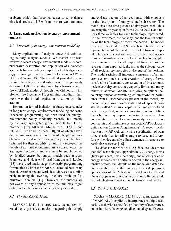
Fig. 1. Event tree for stochastic MARKAL Example: each realization represents a particular cumulative GHG abatement level.
It is based on the multi-stage Stochastic Programmingparadigm, Dantzig [3], Wets [24]. The main charac-teristics of this formulation are summarized below:
1. At each period, there are as many replications ofthe MARKAL variables as there are di�erent sce-nario realizations. At those periods when there aremore than one realization (e.g. at periods 4–9 inthe example shown in Fig. 1), each variable setshould be considered as a set of conditional vari-ables, i.e. variables representing contingent actionswhich will be taken only if the corresponding real-ization prevails.
2. Each set of variables corresponding to a possiblescenario realization must satisfy all MARKALconstraints. Therefore, whatever scenario eventu-ally realizes, the corresponding set of variables(strategy) is feasible. The multi-period constraints,such as capacity transfer, cumulative emission andcumulative resource usage, are thus de�ned in mul-tiple copies, one copy along each path of the eventtree (each such path represents one scenario real-ization). The single-period constraints are repeated
as many times as there are di�erent realizations atthat period, and that number di�ers with the period.
3. The objective function (expected cost) is equalto the weighted sum of the individual scenarioobjective functions (costs), the weight being thescenario’s probability of occurrence.
The formulation described above has been imple-mented on the ExtendedMARKALmodel for Qu�ebec,Kanudia and Loulou [12]. The model has a user in-terface, MUSS (MARKAL Users Support System,Goldstein [7]), which manages the input data andgenerates the linear program for the model. The Ex-tended MARKAL uses OMNI for matrix generation.The existing interface (MUSS) has been extendedto capture the event tree probabilities and the di�er-ent levels of end-use demands and GHG emissionlimits. Extensive modi�cations have been made inthe OMNI code to generate the required stochasticprogram. A new report writer collects the appropriatevariables and compiles the results for each scenario.These developments constitute a user-friendly soft-ware, which can be used to quickly make runs withdi�erent assumptions and easily analyze the results.
224 R. Loulou, A. Kanudia /Operations Research Letters 25 (1999) 219–230
3.4. Implementation of the Minimax Regretformulation
The implementation of the MMR program de-scribed by (3) draws heavily from that of StochasticMARKAL described above. The �rst two character-istics of the formulation, that is the replication ofvariables and constraints, remain the same. However,the third characteristic di�ers: the objective functionis replaced by a single variable �, de�ned in (3),and the �rst series of constraints in (3) are generatedvia an additional manipulation of the MPS �le of theMARKAL program. The objective function valuesfor perfect information runs, M (z), are computedseparately (by solving a deterministic MARKAL pro-gram), and used in the right-hand sides of these con-straints. The FoxPro program used to create the MPS�le for (3) takes about 10 min to transform a 28,000rows-40,000 column problem, on a Pentium-133 ma-chine. The resulting linear program is solved usingCPLEX.As illustrated by Fig. 1, we have selected a range
of cumulative GHG abatement from 0% to 40% ofthe observed 1990 emissions. A cumulative abatementtarget of x% means that, over the 45 year horizon, theaverage yearly emission must be x% lower than theobserved emission in 1990.We now establish that the selected range is indeed
compatible with the recent Kyoto Protocol, which es-tablishes the Canadian abatement percentage at 6%,but for the average emission in the period 2008–2012only. The Protocol says nothing about emissions atother periods. It is conceivable that abatement beyond2012 could be set at levels lower or higher than 6% of1990 emissions (Fankhauser [4]). Such uncertainty isnot easy to resolve to-day, and depends not only on abetter understanding of the seriousness of the impactsof climate change, but also on the dynamics of in-ternational negotiations. Furthermore, in addition tothe post-2012 uncertainty, it is not even certain thatCanada will be reaching the 6% reduction target in2008–2012. Finally, a 6% reduction target for Canadadoes not necessarily translate into a 6% reduction foran individual province such as Quebec. Our uncer-tainty range therefore, although fairly broad, appearsby no means to be too broad. The weak 0% reductiontarget corresponds to a situation where there would benew evidence that the climate change is not as severe
as predicted to-day, and=or that the e�ects of climatechange are not as dramatic or imminent as thought. Atthe upper end, the severe 40% reduction target is notreally as high as it may appear at �rst sight. Indeed, ithas been established [10] that if a stabilization of theCO2 concentration at twice the pre-industrial level(i.e. at 550 ppmv) is desired, world emissions wouldhave to be abated considerably more severely than atthe rate prescribed in the Kyoto Protocol for 2010.The three intermediate targets (10%, 20%, and 30%)are evenly spread over the range. Note that, in view ofthe conjecture of Section 2.3, the intermediate valuesare irrelevant in determining the MMR strategy. Theyare however relevant to compute an optimal strategyunder the expected cost criterion.
4. Analysis of results
4.1. Costs and Regrets of the various Strategies
In our study, seven strategies were examined andcompared: the Minimax Regret strategy (MMR), theMinimum Expected Cost strategy (MEV), and �veshort-sighted strategies. The MEV strategy was stud-ied under the Laplace Criterion, which assumes equal0.2 probability for all �ve targets, a traditional wayre ecting complete uncertainty on the �ve outcomes.Each short-sighted strategy assumes a �xed determin-istic target, until the resolution date, at which time thestrategy is altered to optimally follow whichever targetactually realizes. We call these short-sighted strategiesPerfect Foresight (PF), for lack of a better term. Theyhave been included in the comparison to demonstratethat ignoring uncertainties (i.e. following a PF strat-egy) is in general not a good idea. Carefully note thata PF strategy is not at all the same as the perfect infor-mation (PI) strategy described further down, althougheach PF strategy follows one PI branch up to time t∗.For each combination of the seven strategies and the
�ve possible target realizations, Table 1 indicates thecorresponding cost, as well as the regret. The regret isobtained (as described in Section 2) as the di�erencebetween the cost of the strategy and that of the bestpossible strategy under perfect information. Table 1also indicates the Maximum Regret, as well as the Ex-pected Cost of each strategy (see the last columns).The cost of a PF strategy was derived by running the

R. Loulou, A. Kanudia /Operations Research Letters 25 (1999) 219–230 225
Table 1Objective function values and regrets with 0, 10, 20, 30 and 40% scenarios
System costScenario realization
Strategy 0% Red. 10% Red. 20% Red. 30% Red. 40% Red. Expected value
PF 0% Red. 1 248 297 1 251 024 1 257 793 1 271 067 1 391 320a 1 283 900PF 10% Red. 1 248 611 1 250 385 1 255 863 1 266 496 1 340 820 1 272 435PF 20% Red. 1 249 674 1 250 793 1 255 079 1 264 183 1 296 129 1 263 172PF 30% Red. 1 251 599 1 252 220 1 255 663 1 263 651 1 282 896 1 261 206PF 40% Red. 1 257 480 1 257 728 1 259 781 1 265 676 1 278 261 1 263 785MEV 1251 823 1 252 503 1 255 890 1 263 739 1 281 284 1 261 048MMR 1251 608 1 252 395 1 255 916 1 263 864 1 281 569 1 261 070
RegretsScenario realization
Strategy 0% Red. 10% Red. 20% Red. 30% Red. 40% Red. Max. regret
PF 0% Red. 0 639 2714 7416 113 059 113 059PF 10% Red. 314 0 784 2845 62 559 62 559PF 20% Red. 1377 408 0 532 17 868 17 868PF 30% Red. 3302 1835 584 0 4635 4635PF 40% Red. 9183 7343 4702 2025 0 9183MEV 3526 2118 811 88 3023 3526MMR 3311 2010 837 213 3308 3311
aThis value is for 38% reduction. It is infeasible to implement a 40% reduction target if the 0% strategy is followed till the year 2010.
model in two steps as follows: we illustrate the stepsby computing the real cost of the strategy that followsthe optimal 10% reduction, but when the 20% targetrealizes. First step: the regular MARKAL model isrun with a 10% deterministic target, and obtains anobjective function value of 1250385 M$. Second step:the variables for the �rst three periods are all frozenas per the solution obtained in step 1, and the modelis run again with a 20% constraint, to get the value1255863 M$, which is the real cost of the 10% PFstrategy followed when 20% target realizes. The sameprocedure is applied to all PF strategies and all possi-ble realizations.Fig. 2 shows essentially the same information as
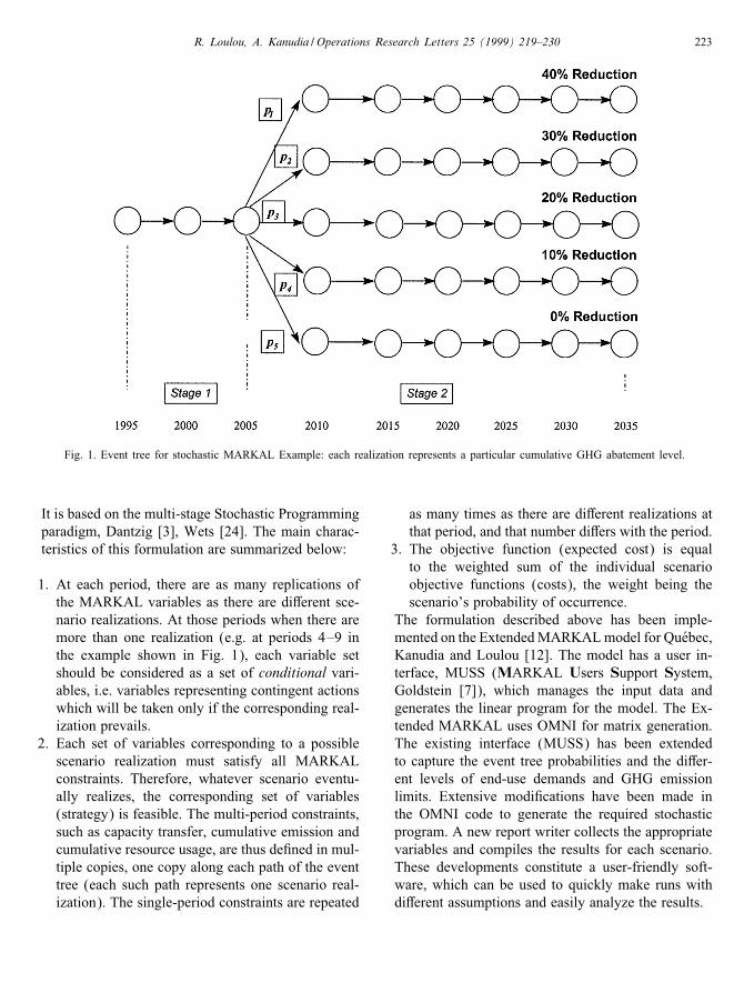
Table 1, but in the graphical form of cost-emissiontrade-o� curves. Note that the “strategy” PI (alsocalled Ideal Strategy), represented by the dotted line,is actually not a realistic strategy since it assumesthat perfect information is available before the �rstperiod starts. It is only used as a benchmark to eval-uate the hedging strategies. For any given target, thevertical di�erence in cost between any strategy andPI is precisely the regret attached to the strategy.
From these results, it is evident that none of thePF strategies performs nearly as well as the MMR orthe MEV strategies on the minimax regret criterion.The best of the PF strategies is to follow the 30%target until resolution date, with a worst regret of M$4635, i.e. M$ 1322 larger than the MMR worst regret.However, the MEV and MMR strategies appear veryclose to each other (their worst regrets are 3526 and3311 M$, respectively, and their expected costs areonly 22 M$ apart).
4.2. Sensitivity analysis
In order to verify whether the closeness of the twoapproaches was accidental or systematic, we con-ducted two sensitivity analysis experiments. In the�rst of these, we adopted a coarser range of targets,namely 0%, 20%, and 40% (Table 2). Of course, thisdid not change the results for MMR, in view of theconjecture. However, the maximum regret of MEVincreased to 4035 M$, i.e. 724 M$ more than theMMR regret. Conversely, the expected costs of thetwo strategies remained close to one another, with a
226 R. Loulou, A. Kanudia /Operations Research Letters 25 (1999) 219–230
Fig. 2. Cost-emission trade-o� curves with 0, 10, 20, 30 and 40% scenarios.
Table 2Objective function values and regrets with 0, 20 and 40% scenarios
System costScenario realization
Strategy 0% Red. 20% Red. 40% Red. Expected value
PF 0% Red. 1 248 297 1 257 793 1 391 320∗ 1 299 137PF 20% Red. 1 249 674 1 255 079 1 296 129 1 266 961PF 40% Red. 1 257 480 1 259 781 1 278 261 1 265 174MEV 1252 332 1 256 180 1 280 255 1 262 922MMR regret 1 251 608 1 255 916 1 281 569 1 263 031
RegretsScenario realization
Strategy 0% Red. 20% Red. 40% Red. Max. regret
PF 0% Red. 0 2714 113 059 113 059PF 20% Red. 1377 0 17 868 17 868PF 40% Red. 9183 4702 0 9183MEV 4035 1101 1994 4035MMR regret 3311 837 3308 3311
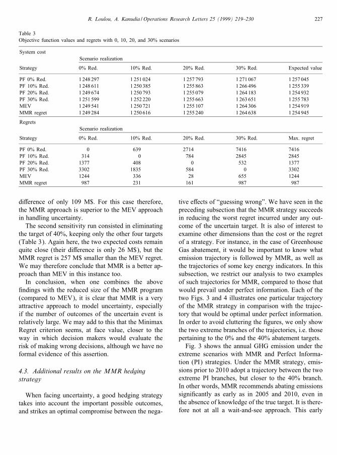
R. Loulou, A. Kanudia /Operations Research Letters 25 (1999) 219–230 227
Table 3Objective function values and regrets with 0, 10, 20, and 30% scenarios
System costScenario realization
Strategy 0% Red. 10% Red. 20% Red. 30% Red. Expected value
PF 0% Red. 1 248 297 1 251 024 1 257 793 1 271 067 1 257 045PF 10% Red. 1 248 611 1 250 385 1 255 863 1 266 496 1 255 339PF 20% Red. 1 249 674 1 250 793 1 255 079 1 264 183 1 254 932PF 30% Red. 1 251 599 1 252 220 1 255 663 1 263 651 1 255 783MEV 1249 541 1 250 721 1 255 107 1 264 306 1 254 919MMR regret 1 249 284 1 250 616 1 255 240 1 264 638 1 254 945
RegretsScenario realization
Strategy 0% Red. 10% Red. 20% Red. 30% Red. Max. regret
PF 0% Red. 0 639 2714 7416 7416PF 10% Red. 314 0 784 2845 2845PF 20% Red. 1377 408 0 532 1377PF 30% Red. 3302 1835 584 0 3302MEV 1244 336 28 655 1244MMR regret 987 231 161 987 987
di�erence of only 109 M$. For this case therefore,the MMR approach is superior to the MEV approachin handling uncertainty.The second sensitivity run consisted in eliminating
the target of 40%, keeping only the other four targets(Table 3). Again here, the two expected costs remainquite close (their di�erence is only 26 M$), but theMMR regret is 257 M$ smaller than the MEV regret.We may therefore conclude that MMR is a better ap-proach than MEV in this instance too.In conclusion, when one combines the above
�ndings with the reduced size of the MMR program(compared to MEV), it is clear that MMR is a veryattractive approach to model uncertainty, especiallyif the number of outcomes of the uncertain event isrelatively large. We may add to this that the MinimaxRegret criterion seems, at face value, closer to theway in which decision makers would evaluate therisk of making wrong decisions, although we have noformal evidence of this assertion.
4.3. Additional results on the MMR hedgingstrategy
When facing uncertainty, a good hedging strategytakes into account the important possible outcomes,and strikes an optimal compromise between the nega-
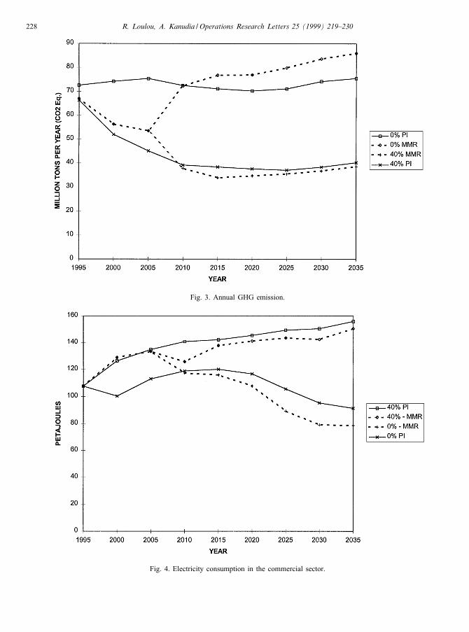
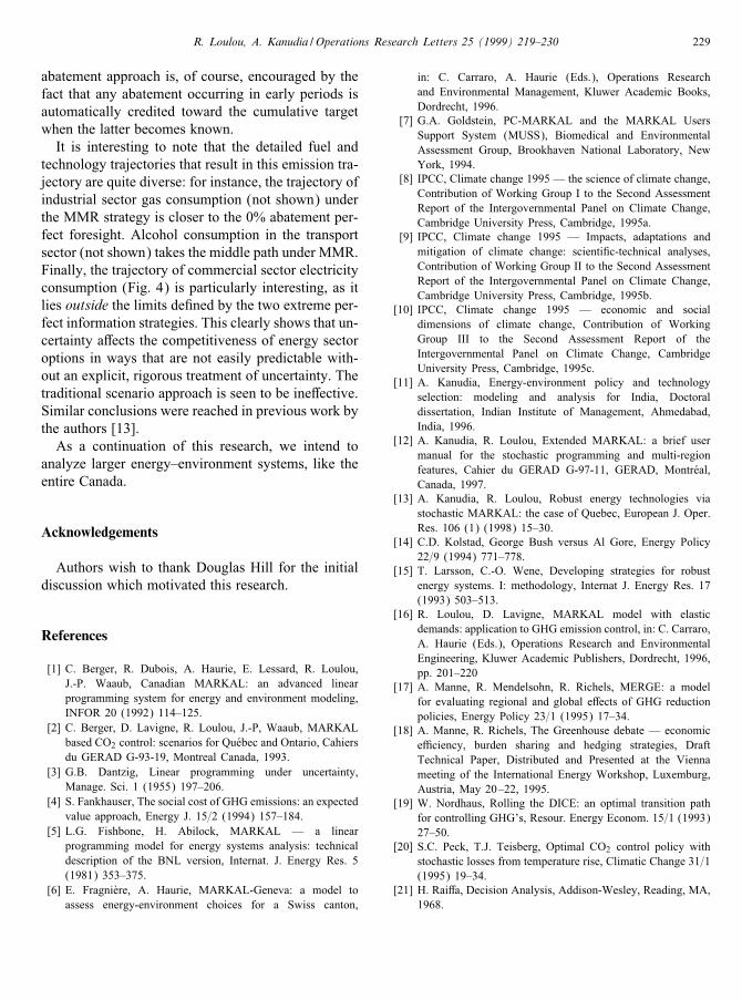
tive e�ects of “guessing wrong”. We have seen in thepreceding subsection that the MMR strategy succeedsin reducing the worst regret incurred under any out-come of the uncertain target. It is also of interest toexamine other dimensions than the cost or the regretof a strategy. For instance, in the case of GreenhouseGas abatement, it would be important to know whatemission trajectory is followed by MMR, as well asthe trajectories of some key energy indicators. In thissubsection, we restrict our analysis to two examplesof such trajectories for MMR, compared to those thatwould prevail under perfect information. Each of thetwo Figs. 3 and 4 illustrates one particular trajectoryof the MMR strategy in comparison with the trajec-tory that would be optimal under perfect information.In order to avoid cluttering the �gures, we only showthe two extreme branches of the trajectories, i.e. thosepertaining to the 0% and the 40% abatement targets.Fig. 3 shows the annual GHG emission under the
extreme scenarios with MMR and Perfect Informa-tion (PI) strategies. Under the MMR strategy, emis-sions prior to 2010 adopt a trajectory between the twoextreme PI branches, but closer to the 40% branch.In other words, MMR recommends abating emissionssigni�cantly as early as in 2005 and 2010, even inthe absence of knowledge of the true target. It is there-fore not at all a wait-and-see approach. This early
228 R. Loulou, A. Kanudia /Operations Research Letters 25 (1999) 219–230
Fig. 3. Annual GHG emission.
Fig. 4. Electricity consumption in the commercial sector.
R. Loulou, A. Kanudia /Operations Research Letters 25 (1999) 219–230 229
abatement approach is, of course, encouraged by thefact that any abatement occurring in early periods isautomatically credited toward the cumulative targetwhen the latter becomes known.It is interesting to note that the detailed fuel and
technology trajectories that result in this emission tra-jectory are quite diverse: for instance, the trajectory ofindustrial sector gas consumption (not shown) underthe MMR strategy is closer to the 0% abatement per-fect foresight. Alcohol consumption in the transportsector (not shown) takes the middle path under MMR.Finally, the trajectory of commercial sector electricityconsumption (Fig. 4) is particularly interesting, as itlies outside the limits de�ned by the two extreme per-fect information strategies. This clearly shows that un-certainty a�ects the competitiveness of energy sectoroptions in ways that are not easily predictable with-out an explicit, rigorous treatment of uncertainty. Thetraditional scenario approach is seen to be ine�ective.Similar conclusions were reached in previous work bythe authors [13].As a continuation of this research, we intend to
analyze larger energy–environment systems, like theentire Canada.
Acknowledgements
Authors wish to thank Douglas Hill for the initialdiscussion which motivated this research.
References
[1] C. Berger, R. Dubois, A. Haurie, E. Lessard, R. Loulou,J.-P. Waaub, Canadian MARKAL: an advanced linearprogramming system for energy and environment modeling,INFOR 20 (1992) 114–125.
[2] C. Berger, D. Lavigne, R. Loulou, J.-P, Waaub, MARKALbased CO2 control: scenarios for Qu�ebec and Ontario, Cahiersdu GERAD G-93-19, Montreal Canada, 1993.
[3] G.B. Dantzig, Linear programming under uncertainty,Manage. Sci. 1 (1955) 197–206.
[4] S. Fankhauser, The social cost of GHG emissions: an expectedvalue approach, Energy J. 15=2 (1994) 157–184.
[5] L.G. Fishbone, H. Abilock, MARKAL — a linearprogramming model for energy systems analysis: technicaldescription of the BNL version, Internat. J. Energy Res. 5(1981) 353–375.
[6] E. Fragni�ere, A. Haurie, MARKAL-Geneva: a model toassess energy-environment choices for a Swiss canton,
in: C. Carraro, A. Haurie (Eds.), Operations Researchand Environmental Management, Kluwer Academic Books,Dordrecht, 1996.
[7] G.A. Goldstein, PC-MARKAL and the MARKAL UsersSupport System (MUSS), Biomedical and EnvironmentalAssessment Group, Brookhaven National Laboratory, NewYork, 1994.
[8] IPCC, Climate change 1995 — the science of climate change,Contribution of Working Group I to the Second AssessmentReport of the Intergovernmental Panel on Climate Change,Cambridge University Press, Cambridge, 1995a.
[9] IPCC, Climate change 1995 — Impacts, adaptations andmitigation of climate change: scienti�c-technical analyses,Contribution of Working Group II to the Second AssessmentReport of the Intergovernmental Panel on Climate Change,Cambridge University Press, Cambridge, 1995b.
[10] IPCC, Climate change 1995 — economic and socialdimensions of climate change, Contribution of WorkingGroup III to the Second Assessment Report of theIntergovernmental Panel on Climate Change, CambridgeUniversity Press, Cambridge, 1995c.
[11] A. Kanudia, Energy-environment policy and technologyselection: modeling and analysis for India, Doctoraldissertation, Indian Institute of Management, Ahmedabad,India, 1996.
[12] A. Kanudia, R. Loulou, Extended MARKAL: a brief usermanual for the stochastic programming and multi-regionfeatures, Cahier du GERAD G-97-11, GERAD, Montr�eal,Canada, 1997.
[13] A. Kanudia, R. Loulou, Robust energy technologies viastochastic MARKAL: the case of Quebec, European J. Oper.Res. 106 (1) (1998) 15–30.
[14] C.D. Kolstad, George Bush versus Al Gore, Energy Policy22=9 (1994) 771–778.
[15] T. Larsson, C.-O. Wene, Developing strategies for robustenergy systems. I: methodology, Internat J. Energy Res. 17(1993) 503–513.
[16] R. Loulou, D. Lavigne, MARKAL model with elasticdemands: application to GHG emission control, in: C. Carraro,A. Haurie (Eds.), Operations Research and EnvironmentalEngineering, Kluwer Academic Publishers, Dordrecht, 1996,pp. 201–220
[17] A. Manne, R. Mendelsohn, R. Richels, MERGE: a modelfor evaluating regional and global e�ects of GHG reductionpolicies, Energy Policy 23=1 (1995) 17–34.
[18] A. Manne, R. Richels, The Greenhouse debate — economice�ciency, burden sharing and hedging strategies, DraftTechnical Paper, Distributed and Presented at the Viennameeting of the International Energy Workshop, Luxemburg,Austria, May 20–22, 1995.
[19] W. Nordhaus, Rolling the DICE: an optimal transition pathfor controlling GHG’s, Resour. Energy Econom. 15=1 (1993)27–50.
[20] S.C. Peck, T.J. Teisberg, Optimal CO2 control policy withstochastic losses from temperature rise, Climatic Change 31=1(1995) 19–34.
[21] H. Rai�a, Decision Analysis, Addison-Wesley, Reading, MA,1968.

230 R. Loulou, A. Kanudia /Operations Research Letters 25 (1999) 219–230
[22] L.A. Terry, M.V.F. Pareira, T.A. Araripe Neto, L.F.C.A.Silva, P.R.H. Sales, Coordinating the energy generation of theBrazilian national hydrothermal generation system, Interfaces16/1 (1986) 16–38.
[23] C.-O. Wene, Investigating robustness with MARKAL, ReportPresented to the IEA=CRD Ad Hoc Group on StrategyDevelopment in Stockholm, July 1979. Reprinted as Report
A82-117, Department of Energy Conversion, ChalmersUniversity of Technology, G�oteborg, Sweden, 1986.
[24] R.J.B. Wets, Stochastic programming, in: L. NemhauserGeorge, K. Rinnooy, H.G. Alexander, J. Todd Michael(Eds.), Handbooks in OR and MS, Vol. 1, Elsevier SciencePublishers, Amsterdam, 1989.