Embed Size (px)
Citation preview

European Network ofTransmission System Operators
for Electricity
Mid-term Adequacy Forecast Appendix 2Methodology 2020 Edition
Mid-term Adequacy Forecast 2020
ENTSO-E AISBL • Rue de Spa 8 • 1000 Brussels • Belgium • Tel + 32 2 741 09 50 • Fax + 32 2 741 09 51 • [email protected] • www. entsoe.eu
1
Table of Contents
1 Mid-term adequacy forecast methodology .............................................................................. 2
1.1 Time horizon and resolution .............................................................................................................3
1.2 Geographical scope ..........................................................................................................................3
1.3 Main assumptions .............................................................................................................................4
1.4 Main inputs and uncertainties ...........................................................................................................5
Generation side .........................................................................................................................5
Grid side ...................................................................................................................................6
Demand side .............................................................................................................................6
1.5 Putting the pieces together................................................................................................................7
General workflow .....................................................................................................................7
Optimisation .............................................................................................................................9
1.6 Adequacy and convergence ............................................................................................................11
Adequacy indices....................................................................................................................11
Model Convergence................................................................................................................12
National reliability standards ..................................................................................................13
2 Databases and tools used for the MAF................................................................................. 15
2.1 PEMMDB .......................................................................................................................................15
2.2 TRAPUNTA ...................................................................................................................................15
2.3 PECD ..............................................................................................................................................15
3 Current methodology: Limitations of MAF 2020 .................................................................... 16
4 ERAA methodology and gap analysis .................................................................................. 17
4.1 Economic viability assessment .......................................................................................................18
Economic viability assessment: Methodology and proof of concept .....................................18
Additional revenues ................................................................................................................20
Preliminary simulations and next steps ..................................................................................20
4.2 Implementation of flow-based market coupling: Definition of the target methodology and proof of
concept .......................................................................................................................................................20
Methodology description ........................................................................................................21
Preliminary simulations ..........................................................................................................24
Conclusions and outlook ........................................................................................................24

Mid-term Adequacy Forecast 2020
ENTSO-E AISBL • Rue de Spa 8 • 1000 Brussels • Belgium • Tel + 32 2 741 09 50 • Fax + 32 2 741 09 51 • [email protected] • www. entsoe.eu
2
1 Mid-term adequacy forecast methodology
Adequacy studies aim to evaluate a power system’s available resources and projected electricity demand to
identify supply/demand mismatch risks under a variety of scenarios. In an interconnected power system such
as the European system, this scope should be extended by considering the supply and demand balance under
a defined network infrastructure, which can have a considerable impact on adequacy results. In this context,
the focus of a pan-European Mid-Term Adequacy Forecast (MAF) - as presented in the current report by
ENTSO-E - assesses the adequacy of supply to meet demand in the mid-term time horizon while considering
the connections between different power systems across the European perimeter, as illustrated in Figure 1.
Figure 1: The interconnected European power system modelled in MAF 2020 (Note: Burshtyn Island in Ukraine is also
explicitly modelled in MAF 2020)
The present MAF probabilistic methodology is considered a reference within Europe. However, the
methodology followed in each MAF report up to the present should be understood as not yet aligned with the
ENTSO-E’s European Resource Adequacy Assessment (ERAA) under the “Clean Energy for all Europeans”
legislative package (see Section 4). Notably, both the MAF 2020 scenarios and results should not be
interpreted or utilised under this new legal framework. The present analysis is not a forecast of actual scarcity
situations, but rather an indication of a range of possible realisations. As such, the actual realisation of future
scarcity events could be very different.

Mid-term Adequacy Forecast 2020
ENTSO-E AISBL • Rue de Spa 8 • 1000 Brussels • Belgium • Tel + 32 2 741 09 50 • Fax + 32 2 741 09 51 • [email protected] • www. entsoe.eu
3
1.1 Time horizon and resolution
A mid-term assessment of adequacy can focus on a single year or multiple years in the future to highlight
supply shortage risks and thus assist stakeholders in making well-informed investment decisions. Notably, it
considers techno-economic trends and policy decisions (e.g. a massive phase-out of certain generation
technologies). The MAF 2020 focuses on target years (TYs) 2025 and 2030.
An hourly resolution has been adopted for the simulations of both TYs, meaning that all input time series
data for the unit commitment and economic dispatch (UCED) model (e.g., RES generation, demand profiles
and net transfer capacities) are expressed in hourly intervals.
1.2 Geographical scope The present study focuses on the pan-European perimeter and neighbouring zones connected to the European
power system. Zones can modelled either explicitly, either non-explicitly. Explicitly modelled zones are
represented by market nodes that consider complete information using the finest available resolution of input
data (e.g., information regarding generating units and demand). Non-explicitly modelled zones are market
nodes for which detailed power system information is not available to ENTSO-E, meaning that only expected
hourly exchanges between these market nodes and adjacent explicit nodes are considered.
Only connections between market/bidding zones are modelled in the MAF model, while intrazonal grid
topology is not. However, some countries have been divided into multiple zones to reflect the effect of certain
critical grid elements (e.g. Greece, Denmark and Italy). Table 1 presents both the explicitly and non-explicitly
modelled zones in MAF 2020, while the explicitly modelled zones are illustrated in Figure 1.
Table 1: Explicitly and non-explicitly modelled zones
Explicitly modelled member countries/regions
Albania (AL00) Finland (FI00) Republic of North Macedonia (MK00)
Slovenia (SI00)
Austria (AT00) France (FR00) Malta (MT00) Spain (ES00)
Belgium (BE00) Germany (DE00) Montenegro (ME00) Sweden (SE01, SE02, SE03, SE04)
Bosnia and Herzegovina (BA00)
Greece (GR00, GR03) Netherlands (NL00) Switzerland (CH00)
Bulgaria (BG00) Hungary (HU00) Norway (N0N1, NOM1, NOS0)
Turkey (TR00)
Croatia (HR00) Ireland (IE00) Poland (PL00) Ukraine Burshtyn Island (UA01)
Cyprus (CY00) Italy (ITN1, ITCN, ITCS, ITS1, ITCA, ITSA, ITSI)
Portugal (PT00) United Kingdom (UK00, UKNI)
Czech Republic (CZ00) Latvia (LV00) Romania (RO00)
Denmark (DKW1, DKE1) Lithuania (LT00) Serbia (RS00)
Estonia (EE00) Luxembourg (LU00) Slovakia (SK00)
Non-modelled member countries/regions
Iceland (IS00)
Implicitly modelled neighbouring countries/regions
Belarus Morocco Russia

Mid-term Adequacy Forecast 2020
ENTSO-E AISBL • Rue de Spa 8 • 1000 Brussels • Belgium • Tel + 32 2 741 09 50 • Fax + 32 2 741 09 51 • [email protected] • www. entsoe.eu
4
1.3 Main assumptions
The MAF model is a simplified representation of the pan-European power system that - like any model - is
based on a set of assumptions, which include:
1) Central planning for generation dispatch: The modelling tools dispatch the generation units for
specified time horizons based on their marginal production cost and other plant parameters. For more
details, see Section 1.5.2.
2) Perfect information during the UCED problem: RES available energy, thermal, demand-side
response (DSR) and grid capacities and demand are known in advance with perfect accuracy;
therefore, there are no deviations from the forecast during their realisation. As such, balancing
reserves are not needed, which is why they are subtracted from the available capacity in the
assessment. Furthermore, perfect foresight is assumed for variables affecting optimal hydro dispatch.
3) Demand is aggregated by region: Individual end users or end-user groups are not modelled.
4) Demand elasticity regarding climate and price: Demand levels are partly correlated to the weather.
For example, temperature variations will affect demand levels due to the use of electrical
heating/cooling devices. A portion of the demand is modelled as DSR, in which load can be reduced
if energy prices are higher than the activation price. The remaining share of energy demand is
regarded as inelastic to price and will thus hold regardless of the energy price.
5) Focus on energy markets only: Capacity markets are not modelled in the MAF. Adequacy is
evaluated from a day-ahead/intraday market perspective. Lack of adequacy, the primary focus of
MAF, should reflect the expectation that the system is not structurally balanced, at least in some
hours and/or days. Additionally, no forward/futures markets or forward/futures contracts between
market players are modelled. As such, these do not influence modelled resource capacities. However,
the effect of capacity markets will be assessed in the context of the ERAA (see Section 4.1).
6) Value of Lost Load (VoLL) is equal among all market areas: Thus, costs associated with unserved
energy (= VoLL) do not differ between market areas. Moreover, it is ensured that the VoLL is higher
than the most expensive production unit/demand flexibility unit in the system.
7) RES production depends on climate: Solar, wind and hydro power generation directly depend on
climate conditions.
8) Forced/unplanned outages only affect thermal generation and grid assets: Thus, a power plant’s
net generating capacity (NGC) and a grid’s net transmission capacity (NTC) are not continuously
guaranteed in a given TY. As seen in Section 1.5.2, forced outages are randomly generated for
thermal assets and grid elements within each modelling tool, while planned grid outages are included
in NTCs provided by the Transport System Operators (TSOs). Lastly, forced outages do not impact
planned outages in any way.
9) Maintenance/planned outages for thermal units are optimised within the modelling tools: While
forced outages occur randomly over time, planned thermal unit maintenance periods are scheduled
during less critical periods (i.e., periods with likely supply surplus rather than supply deficit). The
maintenance optimisation considers country-specific restrictions such as the maximum number of
units simultaneously under maintenance.
10) Some technical parameters of thermal generators are modelled in a simplified manner:
Technical parameters considered to have a low impact on adequacy are modelled in a simplified
manner or neglected (e.g., minimum up/down time [h] restrictions that represent economical
restrictions are not considered). Technical limitations (e.g., maximum ramping [MW/h]) are only

Mid-term Adequacy Forecast 2020
ENTSO-E AISBL • Rue de Spa 8 • 1000 Brussels • Belgium • Tel + 32 2 741 09 50 • Fax + 32 2 741 09 51 • [email protected] • www. entsoe.eu
5
considered immediately after the occurrence of a unit outage. Lastly, marginal costs are assumed to
be constant and independent of the generation level.
11) NTC approach: Electricity exchanges between market nodes are optimised as part of UCED model
optimisation and limited by the respective NTC between the nodes. The NTC approach considers
only bilateral power flows without considering the impact of flows in neighbouring regions. A more
sophisticated approach that also considers the impact of exchanges in neighbouring regions is
explained in Section 4.2 and will be implemented in the context of the ERAA.
1.4 Main inputs and uncertainties
To optimise and forecast a power system’s operation, a large amount of detailed data and information is
required. However, even with the best available data, the results are subject to considerable uncertainty,
thereby resulting in a difficult decision-making process for market players. Fortunately, the impact of such
uncertainty can be reduced thanks to probabilistic market modelling methodologies.
Figure 2: Overview of the methodological approach
Figure 2 illustrates the main elements of the MAF 2020 methodology and their impact on adequacy. The
three pillars of an adequacy assessment include available generation, demand and network infrastructure.
Generation side
In MAF, the forecasted net generation capacities (NGCs) for thermal assets are provided by the TSOs. In this
methodology, thermal generation depends on deterministic planned outages optimised within the MAF (see
Chapter 1.5) and random forced outages that account for plant breakdowns. Planned outage periods for
thermal generation assets are usually scheduled during periods of high expected adequacy (i.e., periods of
low demand). To avoid adequacy risks, planning must respect a certain number of criteria, which include a
maximum number of days per year of maintenance, a ratio of winter vs summer maintenance durations and
the maximum number of thermal units in simultaneous maintenance. A single maintenance planning profile
for each plant is generated and fed into the models.
In MAF, the RES generation levels depend on climate variable profiles and the RES NGCs provided by
TSOs. Solar, wind and hydro generation depend on solar irradiance, wind conditions and hydro inflows,
Mid-term Adequacy Forecast 2020
ENTSO-E AISBL • Rue de Spa 8 • 1000 Brussels • Belgium • Tel + 32 2 741 09 50 • Fax + 32 2 741 09 51 • [email protected] • www. entsoe.eu
6
respectively (see Section 1.5.1). However, hydro assets with storage are a unique case and their operation
schedule is the result of an optimisation (see Section 1.5.2).
Balancing reserves (or ancillary services) are power reserves contracted by TSOs that help stabilise or restore
the grid’s frequency following minor or major disruptions due to factors such as unforeseen plant outages or
higher loads. While they are fundamental to a power system’s stability, only replacement reserves are
modelled in the MAF. Indeed, the MAF measures structural inadequacies that manifest in time steps of 1
hour or longer and does not analyse what occurs within each hour. To avoid scheduling operational reserves
(FCR and FRR) for time steps of 1 hour or longer - thus making them unavailable for their initial purpose -
the latter are not modelled. Doing otherwise would result in severe violations of the frequency quality criteria
outlined in legislation.
From a modelling perspective, reserves can be considered in two ways: by reducing the respective thermal
generation capacity or increasing the demand by adding the hourly reserve capacity requirements. For
practical reasons, the reserves were considered by adding them to consumption rather than applying a thermal
capacity reduction, thereby making it easier to implement the market models. However, doing so has the
disadvantage of distorting the reported energy balance since ‘virtual consumption’ has been added. In some
countries, reserves are provided by hydro generation. In these cases, they are implemented as a constraint on
the maximum hydro generation. In special cases (e.g., where a TSO has agreements with large electricity
users regarding demand reduction when needed or dedicated back-up power plants), the reserve specifications
were directly coordinated with the TSO data correspondent. On the other hand, replacement reserves (RRs)
are considered in the MAF adequacy calculations (i.e., RRs are available to meet demand).
Grid side
Similar to thermal capacities, the forecasted available net transfer capacities are provided by the TSOs with
an hourly resolution. Planned maintenance for the transmission lines was not centrally optimised in MAF
2020 but was considered integrated into the NTC hourly availability, as provided by TSOs. Transmission
levels depend on deterministic planned outages and random forced outages, which are modelled in the same
manner as the generation elements. Interconnectors between the market zones can consist of multiple poles,
which are also explicitly modelled in the MAF. Random outages on these interconnectors are drawn per pole
(i.e., at borders with multiple poles, an outage of one pole does not reduce the NTC to zero).
Demand side
Demand level forecasts are provided by TSOs based on their best estimates regarding electric vehicle
penetration, heat pumps, annual demand levels, etc. The hourly time series, which are required as an input
for the UCED model, are then calculated by ENTSO-E considering the dependence of demand on
temperature. For more information on the generation of the demand time series, see Section 2.2.
In modern unbundled power systems, evaluating adequacy also involves the contribution of elasticity of
demand with respect to prices. Furthermore, the effect of storage facilities (including their market-driven
operation), electric vehicles and heat pumps, along with their corresponding impacts on demand profiles, are
considered.
The DSR is modelled in a simplified manner as a generator that participates in the market. Since each DSR
unit is characterised by an offer quantity and offer price, it can thus be dispatched as part of the merit order
curve. Additionally, the number of hours that the units can operate per day can be limited. Prices, quantities
and operational constraints are delivered by the TSOs and can consist of multiple bands where a price
differentiation is requested. In most countries, DSR units have relatively high prices, which ensures that they
are the last dispatchable services before energy not served (ENS) occurs. However, in some countries, DSR

Mid-term Adequacy Forecast 2020
ENTSO-E AISBL • Rue de Spa 8 • 1000 Brussels • Belgium • Tel + 32 2 741 09 50 • Fax + 32 2 741 09 51 • [email protected] • www. entsoe.eu
7
units can be dispatched before the price-setting generator. Finally, it is ensured that the dispatch price of a
DSR unit is set lower than the VoLL.
1.5 Putting the pieces together
The main feature of the MAF probabilistic methodology is the use of Monte Carlo (MC) sampling to combine
different climate conditions through climate-dependent variables and random forced outages on generation
assets and interconnections for a given TY, as visualised in Figure 3.
Initially, climate years from 1982 to 2016 are selected one-by-one (N climate years). These include
temperature-dependent demand time series, wind and solar load factor time series and hydro inflow time
series. Each set of climate conditions is further associated with a relatively large number of random forced
outage realisation samples (M outage samples) (i.e., randomly assigning forced outage patterns to thermal
generating units and interconnections (high-voltage direct current (HVDC) and some high-voltage alternating
current (HVAC))). Notably, random forced outages do not affect planned outages in the models. The number
of random forced outage patterns M is not known until model convergence has been reached (more details
on the convergence can be found in Section Fehler! Verweisquelle konnte nicht gefunden werden.).
Figure 3: Monte Carlo simulation principles for a given target year
As will be shown further below, the MAF methodology uses five modelling tools to improve results reliability
and robustness. Each tool solves its own system cost minimisation problem for a given TY (also known as a
UCED problem) and derives the marginal energy market price. Each tool also attempts to find the least-cost
solution while respecting operational constraints such as minimum stable feed-in level, transfer capacity
limits and so on. Most optimisation solvers and computers are capable of solving single large-scale mixed-
integer linear programming (MILP) problems within acceptable computation times; however, the very large
number of MC simulations (NxM) makes the MAF a time-intensive and challenging task. Since integer
constraints are simplified in MAF 2020, the final problem to be solved is a linear programming (LP) problem.
General workflow
Figure 4 and Figure 5 illustrate the current MAF workflow to build and combine model inputs with the
optimisation and convergence workflow.
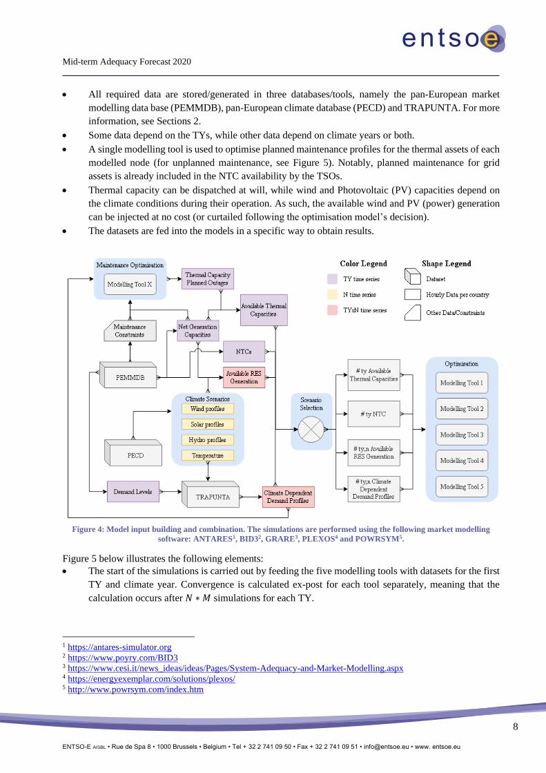
Briefly, Figure 4 below illustrates the following elements:
Mid-term Adequacy Forecast 2020
ENTSO-E AISBL • Rue de Spa 8 • 1000 Brussels • Belgium • Tel + 32 2 741 09 50 • Fax + 32 2 741 09 51 • [email protected] • www. entsoe.eu
8
• All required data are stored/generated in three databases/tools, namely the pan-European market
modelling data base (PEMMDB), pan-European climate database (PECD) and TRAPUNTA. For more
information, see Sections 2.
• Some data depend on the TYs, while other data depend on climate years or both.
• A single modelling tool is used to optimise planned maintenance profiles for the thermal assets of each
modelled node (for unplanned maintenance, see Figure 5). Notably, planned maintenance for grid
assets is already included in the NTC availability by the TSOs.
• Thermal capacity can be dispatched at will, while wind and Photovoltaic (PV) capacities depend on
the climate conditions during their operation. As such, the available wind and PV (power) generation
can be injected at no cost (or curtailed following the optimisation model’s decision).
• The datasets are fed into the models in a specific way to obtain results.
Figure 4: Model input building and combination. The simulations are performed using the following market modelling
software: ANTARES1, BID32, GRARE3, PLEXOS4 and POWRSYM5.
Figure 5 below illustrates the following elements:
• The start of the simulations is carried out by feeding the five modelling tools with datasets for the first
TY and climate year. Convergence is calculated ex-post for each tool separately, meaning that the
calculation occurs after 𝑁 ∗ 𝑀 simulations for each TY.
1 https://antares-simulator.org 2 https://www.poyry.com/BID3 3 https://www.cesi.it/news_ideas/ideas/Pages/System-Adequacy-and-Market-Modelling.aspx 4 https://energyexemplar.com/solutions/plexos/ 5 http://www.powrsym.com/index.htm

Mid-term Adequacy Forecast 2020
ENTSO-E AISBL • Rue de Spa 8 • 1000 Brussels • Belgium • Tel + 32 2 741 09 50 • Fax + 32 2 741 09 51 • [email protected] • www. entsoe.eu
9
• Reaching model convergence for a given TY is an iterative process. Initially, the modellers must decide
on an initial amount of random outage patterns M to be generated by each modelling tool. Each tool
generates its own distinctive patterns respecting a set of criteria and optimises the model for each
pattern. If convergence is not reached, M is increased for the models that did not converge.
Figure 5: Model optimisation and convergence process.
Optimisation
An additional optimisation step for hydro storage assets occurs within each modelling tool after forced outage
pattern generation and before the UCED optimisation. The available energy profile of hydro storage assets is
optimised in weekly or monthly resolution steps so that energy is available for turbining in times of
simultaneous high demand and low available generation, while it is pumped (in the case of pump storage
units) or stored (in the case of hydro storage units without a pumping facility) in times of oversupply.
Simultaneously, exogenously provided weekly or monthly energy targets constrain the optimisation.
The UCED optimisation is then performed in smaller time steps (e.g., one day) to determine which units are
dispatched at each hour of the optimisation horizon and the respective dispatch level. For the optimisation, a
given TY is divided into several UCED optimisation time steps/horizons. Each resulting UCED problem is

Mid-term Adequacy Forecast 2020
ENTSO-E AISBL • Rue de Spa 8 • 1000 Brussels • Belgium • Tel + 32 2 741 09 50 • Fax + 32 2 741 09 51 • [email protected] • www. entsoe.eu
10
optimised based on its profiles of available thermal NGC, RES available energy, grid NTCs and demand.
Then, each UCED problem is given the final system state of the preceding UCED problem (used as the initial
dispatching state for the current UCED problem). Indeed, optimising a given UCED problem with a different
initial dispatching state while keeping other parameters unchanged may yield different results. Similarly,
dividing a TY into a different number of UCED problems may yield different results.
Figure 6: Illustration of the MAF modelling process
Currently, the network modelling approach for pan-European or regional market studies is based on NTC
market coupling (a zonal model), which implies that the network constraints between market nodes are
modelled not as physical limits, but as commercial exchange limits at the border (i.e., the available capacity
for commercial exchanges as opposed to the total transfer capacity). This approach is also followed in the
current study, while the value of NTC can differ throughout the year and comprises an hourly time series of
NTC for each interconnection throughout each modelled TY.

Mid-term Adequacy Forecast 2020
ENTSO-E AISBL • Rue de Spa 8 • 1000 Brussels • Belgium • Tel + 32 2 741 09 50 • Fax + 32 2 741 09 51 • [email protected] • www. entsoe.eu
11
1.6 Adequacy and convergence
Adequacy indices
System adequacy refers to the existence of sufficient resources to meet consumers’ demands and the operating
requirements of the power system. The so-called adequacy indicators can be deterministic or probabilistic
metrics, according to the methodologies used for the adequacy assessments.
Regarding the definitions and scope of the indices used in adequacy studies, three main functional zones of
power systems are involved in the adequacy evaluation:
• Generation adequacy level (hierarchical level I), which considers the total system generation and the
effects of transmission constraints in the form of NTCs.
• Transmission adequacy level (hierarchical level II), which includes both the generation and
transmission facilities.
• Overall hierarchical adequacy level (hierarchical level III), which involves all three functional zones,
from the generating points to the individual consumer load points, which are typically connected at the
distribution level.
Traditionally, the adequacy indices can have different designations depending on the hierarchical levels
involved in the adequacy study. In MAF 2020, the focus is on hierarchical level I (i.e., the generation
adequacy level).
In probabilistic MC adequacy studies, the typical indicators for adequacy (simulation results) are either the
expected (average) values of a set of a random variable’s outcomes or a percentile of that set, such as expected
unserved energy or the 95th percentile of unserved energy. The set population is equal to 𝑀 ∗ 𝑁 or a given
region, simulation horizon and simulation tool.
The following indices are used to assess the adequacy levels for a given geographical scope and for a given
time horizon (referred to as a simulation year).
• Loss of load event [h] – Represents an hour in a given MC simulation during which the demand after
consideration of demand flexibilities exceeds the available generation and import capacity.
• ENS [GWh/year] – For a single node, the energy not supplied during a single MC sample/simulation
year due to the demand in the node exceeding the combination of available resource capacity and
electricity imports. For a geographical area with multiple nodes, its ENS is the total ENS of all its
nodes. A null ENS suggests that there are no adequacy concerns.
• Expected energy not served (EENS) [GWh/year] – For a given geographical area the mathematical
average of the ENS calculated over the total number of MC sample/simulation years. It is calculated
according to Eq. (1):
𝐸𝐸𝑁𝑆 =1
𝑀𝐶𝑡𝑜𝑡∑ 𝐸𝑁𝑆𝑗
𝑀𝐶𝑡𝑜𝑡𝑗=1 , (1)
where ENSj is the energy not supplied in the jth-MC simulation and 𝑀𝐶𝑡𝑜𝑡 is the total number of MC
simulations.
• Loss of Load Duration (LLD) [h/year] - For a single node, the number of hours during which the
node experiences ENS during a single MC sample/simulation. Notably, the LLD of an MC simulation

Mid-term Adequacy Forecast 2020
ENTSO-E AISBL • Rue de Spa 8 • 1000 Brussels • Belgium • Tel + 32 2 741 09 50 • Fax + 32 2 741 09 51 • [email protected] • www. entsoe.eu
12
can only be reported as an integer number of hours due to the hourly resolution of the simulation. Thus,
it does not indicate the severity of the deficiency or the duration of the loss of load within that hour.
• Loss of load expectation (LOLE) [h/year] - For a given geography, the mathematical average of the
LLDs over the total number of MC sample/simulation years. It is calculated according to Eq. (2):
𝐿𝑂𝐿𝐸 =1
𝑀𝐶𝑡𝑜𝑡∑ 𝐿𝐿𝐷𝑗
𝑀𝐶𝑡𝑜𝑡𝑗=1 , (2)
where LLDj is the loss of load duration in the jth-MC simulation and 𝑀𝐶𝑡𝑜𝑡 is the total number of MC
simulations.
Model Convergence
To obtain confidence in the results, the latter should remain unchanged with an increasing number of MC
simulations. At that point, it can be said that the model has converged. With the number of climate years N
available being finite, a large number of random outage patterns may be required for the model to converge.
In MAF 2020, the convergence of the model is calculated in several steps. Following a set of simulations, the
model’s convergences are assessed and additional simulations using new forced outage patterns are launched.
This process continues until convergence is reached.
While the results provided in the Executive summary and Appendix 1 are presented for each region
separately, the convergence of the model is assessed based on the results of the entire geographical scope.
MAF 2020 uses the coefficient of variation 𝛼 derived from the ENS of the entire geographical scope, as
defined by Eq. (3):
𝛼 =√Var[𝐸𝐸𝑁𝑆])
𝐸𝐸𝑁𝑆, (3)
where 𝐸𝐸𝑁𝑆 is calculated over all MC simulations completed at the moment of assessment and Var[𝐸𝐸𝑁𝑆]
is the variance of the expectation estimate (i.e., Var[𝐸𝐸𝑁𝑆] =Var[𝐸𝑁𝑆]
𝑁).
Figure 7 illustrates an example of an MC model’s 𝛼 evolution and its relative change with an increasing
number of MC simulations. In Figure 7, one can expect no significant changes in 𝛼 past a certain number of
simulations. With no significant changes in 𝛼 expected, thus in the results, no additional simulations are
required. No explicit 𝛼 targets are set to stop the MC simulations. Instead, the decision of whether or not to
launch additional simulations is a compromise between the expected 𝛼 evolution and the required
computational time.

Mid-term Adequacy Forecast 2020
ENTSO-E AISBL • Rue de Spa 8 • 1000 Brussels • Belgium • Tel + 32 2 741 09 50 • Fax + 32 2 741 09 51 • [email protected] • www. entsoe.eu
13
Figure 7: Example of 𝜶 evolution and its relative change with an increasing number of MC samples for a converging model
Notably, certain inputs and parameters can have a significant impact on the results of these indices and their
convergences, including:
• Hydro power modelling;
• NTCs;
• The use/absence of extreme, yet realistic, historical climatic years (e.g., 1985);
• Outages and their modelling, including both maintenance and forced outages6.
National reliability standards
Table 2 presents an overview of the national reliability standards that the individual EU Member States have
applied to assess their national grid adequacy as of the end of 2019. Countries that are not listed do not have
reliability standards in place.
Table 2: National reliability standards applied by EU Member States as of the end of 20197
6 To understand the impact of forced outages, which are random by definition, it is important for all of the tools to use
one commonly agreed upon maintenance schedule. This maintenance schedule should respect the different constraints
specific to the thermal plants in different countries, as provided by TSOs. 7 2019: ACER Market Monitoring Report 2019 – Electricity Wholesale Markets Volume, p. 60,
https://www.acer.europa.eu/Official_documents/Acts_of_the_Agency/Publication/ACER%20Market%20Monitoring
%20Report%202019%20-%20Electricity%20Wholesale%20Markets%20Volume.pdf
1
1,2
1,4
1,6
1,8
2
1 101 201 301 401 501 601
Number of MC simulations
Coefficient of Variation (a)
0
2
4
6
8
10
12
14
16
1 100 199 298 397 496 595 694
Number of MC simulations
Relative change of coefficient of
variation (%)

Mid-term Adequacy Forecast 2020
ENTSO-E AISBL • Rue de Spa 8 • 1000 Brussels • Belgium • Tel + 32 2 741 09 50 • Fax + 32 2 741 09 51 • [email protected] • www. entsoe.eu
14
Member state Type of reliability standard Value Binding (B)/non-binding (NB)
BE8 LOLE 3 h/year B
P95 20 h/year B
CY Reserve margin 189 MW B
DE LOLE 5 h/year NB
DK8 Outage minutes 5 minutes B
FR LOLE 3 h/year NB
GR LOLE 3 h/year NB
IE LOLE 8 h/year B
IT LOLE 3 h/year B
LT LOLE 8 h/year NB
NL LOLE 4 h/year NB
PT8 LOLE 5 h/year B
Load supply index ≥ 1 B
PL LOLE 3 h/year NB
ES Reserve margin/LOLE (see note) NB
UK LOLE 3 h/year B
Some notes regarding Table 2 are provided based on the Acer Market Monitoring Report7:
• Loss of load probability (LOLP) is the probability that available capacity will not be able to cover
demand.
• Load supply index in Portugal refers to the risk of inadequacy at the day-ahead market only.
• The reserve margin in Cyprus is the level of additional capacity readily available during the peak
period of capacity demand.
• In Denmark, the reliability standard is set in ‘outage minutes (OM)’, which are defined as OM =
8760 * 60 * EUE /Demand, where Demand is the annual load and EUE is the expected unserved
energy (i.e., the EENS adjusted to account for the fact that real load shedding occurs at predefined
blocks of energy). OM indicates the expected proportion of the annual load (converted to minutes)
that cannot be delivered due to a lack of adequacy. OM and LOLE are different measures and are
thus not comparable.
• For Germany, the reliability standard has been derived from a threshold presented in the 2019
security of supply monitoring report9. Herein, a LOLP of 0.06 % has been calculated using the cost
of new entry (CONE) and VOLL(CONE/VOLL=50,000 euro/MW/year/10,000
euro/MWh≈0.06%). Thus, the calculated LOLE is 0.06% of 8760 hours ≈ 5 hours.
• The value for Ireland refers to the I-SEM10 and is used for the current capacity mechanism (CM).
• In Spain, a 10% reserve margin (not legally established) was recently used, while a LOLE indicator
is currently under discussion. For the non-mainland territories, there is a requirement of a
maximum LOLP of one day every 10 years, equivalent to a LOLE of 2.4 hours/year.
• The value for the United Kingdom refers to Great Britain only.
8 Reliability standards for BE, BG, DK and PT have been updated to the table contained in the ACER Market Monitoring
Report7 based on more up-to-date data provided by the corresponding TSOs. 9 2019: Definition and monitoring of security of supply on the European electricity markets, p. 39,
https://www.bmwi.de/Redaktion/EN/Publikationen/Studien/definition-and-monitoring-of-security-of-supply-on-the-
european-electricity-markets-from-2017-to-2019.pdf?__blob=publicationFile&v=9 10 I-SEM stands for integrated single electricity market, a wholesale electricity market where electricity is traded in bulk
across the island of Ireland.

Mid-term Adequacy Forecast 2020
ENTSO-E AISBL • Rue de Spa 8 • 1000 Brussels • Belgium • Tel + 32 2 741 09 50 • Fax + 32 2 741 09 51 • [email protected] • www. entsoe.eu
15
LOLE (h/year) is the most common reliability indicator used by EU Member States, with targets typically in
the range of 3–8 h/year. Setting such reliability targets is a sensitive issue since it requires the consideration
of both economic and technical aspects. For instance, these targets could be determined by comparing the
VoLL against the costs of increasing adequacy. According to the methodology requirement for the future
pan-European Resource Adequacy Assessment, LOLE standards will be defined based on this approach from
the ERAA 2021 onward for all European market zones.
2 Databases and tools used for the MAF
The MAF methodology uses data collected from TSOs or generated by internally developed tools, while also
using assumptions collected by TSOs. The following sections describe the databases and tools used in the
MAF assessment.
2.1 PEMMDB
ENTSO-E uses a single source of supply-side and grid data across all of its assessments (i.e., the PEMMDB
containing data collected by TSOs on plant net generation capacities, interconnection capacities, generation
planned outages, etc.). The database is aligned with national development plans and contains data about the
power system according to the best knowledge of the TSOs at the time of data collection. The PEMMDB
contains a highly granular unit-by-unit resolution of European power plants, their technical and economical
parameters, their expected decommissioning dates and the forecasted development of RES capacities.
Moreover, it provides an hourly time series of must-run obligations and the derating of thermal units.
Compared to MAF 2019, a major improvement to the PEMMDB involves a more detailed representation of
batteries and (partly) flexible consumers (i.e., electric vehicles, heat pumps and new technologies).
The aforementioned data was collected for TYs 2020 to 2030 with a yearly resolution.
2.2 TRAPUNTA
To create the forecasted hourly load profiles for each region, ENTSO-E (and thus MAF) uses a single tool
named TRAPUNTA. This tool builds hourly load profile forecasts for all regions (with some exceptions) by
combining information from historical load time series, historical temperature and other climate variables as
well as additional historical data. This methodology incorporates the decomposition of time series into basic
functions using singular value decomposition (SVD). In the second phase, the tool adjusts the forecasted load
time series using bottom-up scenarios provided by the TSOs that reflect the future evolution of the market
(e.g., penetration of heat pumps, electric vehicles and batteries). More information regarding the methodology
for calculating demand time series is provided in the report “Demand forecasting methodology”11.
2.3 PECD
ENTSO-E developed the PECD, which consists of re-analysed hourly weather data and load factors for
variable generation (i.e., wind and solar). PECD datasets are prepared by external experts using industry best
practices, thus ensuring a representative estimation of demand, variable generation and other climate-
dependent variables. Since 2019, the PECD has been extended to include hydro generation data. Based on
re-analysed data concerning hydro inflows, a standardised central methodology has been designed to map
historical inflows of generation data and build a model to project hydro generation, including hydro run-of-
river, hydro reservoirs and pump storage. In 2020, a further improvement was achieved by introducing a
11 Demand methodology document:
https://docstore.entsoe.eu/Documents/SDC%20documents/MAF/2019/Demand%20forecasting%20methodology.pdf

Mid-term Adequacy Forecast 2020
ENTSO-E AISBL • Rue de Spa 8 • 1000 Brussels • Belgium • Tel + 32 2 741 09 50 • Fax + 32 2 741 09 51 • [email protected] • www. entsoe.eu
16
higher granularity of north-sea offshore zones and updating the zone configuration in Belgium. More
information regarding the methodology and relevant assumptions are included in the corresponding document
“Hydro Power Modelling”12.
3 Current methodology: Limitations of MAF 2020
The current MAF methodology relies on an advanced probabilistic market modelling approach. However,
like every modelling approach, it has its inherent limitations. These limitations are presented as follows:
• Upcoming forced outages considered in UCED: Forced outages are randomly generated but are
known at the time of the UCED, with a look-ahead horizon ranging from 1 to 7 days ahead (depending
on the market modelling tool). As such, the units are dispatched accordingly to avoid/minimise loss
of load.
• Thermal asset planned maintenance optimisation: Planned maintenance optimisation of thermal
generation assets is performed independently for isolated market nodes (i.e., it does not yet include
the grid infrastructure).
• DSR limitations: DSR is only modelled as demand reduction potential in the case of high prices,
while shiftable load is not yet considered in the simulations. Shiftable load enables the re-scheduling
of demand from a period with high prices to a period with lower prices (i.e., from a period with higher
adequacy concerns to a period with lower adequacy concerns). Moreover, the current methodology
considers that part of the demand is elastic regarding price but no other criteria (e.g., the generation
mix of a given moment).
• VoLL: Different end-user groups may be characterised by different loss of load values within a
region and across regions.
• Thermal and grid assets are not affected by climate conditions: In reality, thermal and grid assets
capacities may vary with air temperature and humidity, for example.
• Internal grid limitations within a bidding zone are not considered: However, they have been
further investigated in a flow-based study conducted as a sensitivity analysis (explained further in
Section 4.2. This topic requires further development and also needs to consider possible evolutions
of the European market. The future ERAA—to be developed by ENTSO-E pursuant to article 23 of
EU Regulation 2019/943—will need to be based on a methodology that inter-alia provides for the
use of a market model using the flow-based approach, where applicable.
• No forced outages are assumed for RES13 assets: Since MAF 2019, thermal units have assigned
unit-specific forced outages. However, no random outage draws are considered for RES.
• Forced outages are assumed to not affect planned outages: Generation units’ planned outages are
usually scheduled months or years in advance. However, they may still change depending on the
operational/contractual constraints of each plant owner/operator. In reality, if a forced outage occurs
very close to a planned outage, the latter may be moved at a different moment or even merged with
the forced outage.
12 Hydro methodology document:
https://docstore.entsoe.eu/Documents/SDC%20documents/MAF/2019/Hydropower_Modelling_New_database_and_methodology.p
df 13 This includes hydro generation units.

Mid-term Adequacy Forecast 2020
ENTSO-E AISBL • Rue de Spa 8 • 1000 Brussels • Belgium • Tel + 32 2 741 09 50 • Fax + 32 2 741 09 51 • [email protected] • www. entsoe.eu
17
• Sub-hourly fluctuations of demand and RES are not considered: Demand and RES penetration
are currently modelled with an (averaged) hourly resolution so that sub-hourly variations (e.g.,
demand peaks) of these parameters cannot be modelled.
• Economic viability: Assumptions regarding available resource capacity for each TY are only the
best estimate of TSOs for their area of operation, collected following a bottom-up approach. In MAF
2020, the economic performance of generation units is not assessed with respect to either their
economic viability in the TY or the opportunity for expansion (see Section 4.1 for more information).
• Use of NTCs and not flow-based: See Section 4.
• Sectoral Integration: See Section 4.
4 ERAA methodology and gap analysis
The Clean Energy Package (CEP) brings several changes and updates to the methodology used for adequacy
assessment, while the scope of the assessment is significantly extended. However, implementation of the
complete set of changes will gradually occur over the coming years. An overview of the gap analysis
regarding the target methodology and the current status of further developments in the MAF methodology is
shown in Figure 8.
Figure 8: The MAF methodology gap analysis upon considering the legal requirements for the Clean Energy Package
The main features affected by the CEP implementation are summarised below:
1) Probabilistic market modelling approach (MC): The core of the MAF methodology (i.e.,
probabilistic market modelling) already complies with most requirements of the ERAA. The future
adequacy assessment will be required to present more detailed results followed by the level of
convergence of the probabilistic metrics based on a single modelling tool.
2) TYs and temporal resolution: MAF 2020 focuses on two TYs, while the target ERAA methodology
will request to simulate each of the 10 years ahead, while significantly increasing the workload.
Topic MAF 2020 ERAA Methodology Status
Modelling approach Probabilistic Probabilistic100%
Publication frequency Annual Annual100%
Network NTC approach. Testing Flow-Based
approach since 2018
Compliance with Flow-Based approach50%
Target years and time
horizon
2 target years within a 10 year horizon 10 target years within a 10 year horizon25%
Available resource
capacity
Bottom-up expectations Bottom-up expectations followed by
Economic Viability Assessment 25%
Capacity mechanisms No explicit considerations Effect of Capacity Mechanism integrated25%
Sectoral integration None Integration of Power to Gas, Power to
Hydrogen, etc.0%

Mid-term Adequacy Forecast 2020
ENTSO-E AISBL • Rue de Spa 8 • 1000 Brussels • Belgium • Tel + 32 2 741 09 50 • Fax + 32 2 741 09 51 • [email protected] • www. entsoe.eu
18
3) Impact of climate change: The current methodology uses historical climate data for its probabilistic
assessment. These historical data do not account for the impact that climate change could have on
climate variables in the years to come. Thus, the ERAA climate change impact on the climate
variables will be considered an update to the PECD.
4) CMs: Existing, approved or planned CM assets may be included in the assessment as part of the
NGC forecasts of some TSOs. The ERAA will require the impacts of approved, existing and planned
CM assets on adequacy to be studied separately.
5) Sectoral integration: Sectoral integration technologies, such as technologies for power-to-gas and
power-to-hydrogen conversions or power conversions to other mediums, are not accounted for in the
MAF but will be required in the ERAA.
6) Economic viability: The MAF is based on top-down scenarios for installed capacities and does not
consider the economic viability of the fleet. Only expected or official commissioning and
decommissioning dates of thermal generation plants are considered when building the MAF
scenarios. The CEP requires the incorporation of an investment module, which will assess the
economic viability of capacity resources and their potential exit from the market (see Section 4.1).
7) Flow-based: The MAF is built on the NTC approach for the representation of grid elements.
However, it will be replaced by flow-based market coupling (FBMC), which is one of the target
features of the future adequacy assessments (see Section 4.2).
4.1 Economic viability assessment
Economic viability assessment: Methodology and proof of concept
An economic viability assessment (EVA) is a methodological element in the target ERAA methodology that
aims to identify changes in the capacity mix stemming from economic reasons that could affect the likelihood
of retirement, mothballing and new investments in capacity. In the current MAF state of play, TSOs provide
their best estimates of available units for each of the simulated TYs based on national plans and/or ambitions
and the best available knowledge at the time of data collection. However, the economic rationale that would
ensure that these capacities would indeed materialise is not verified, rendering such assumptions intrinsically
uncertain. Additionally, even if these estimates could be realised, they may represent a non-optimal asset mix
with regard to profitability. The EVA aims to identify assets that, under perfect competition, would likely be
decommissioned or mothballed while simultaneously identifying potential new generation investments.
Additionally, under the ERAA, the ability of existing CMs to improve adequacy for a given TY is taken into
account by assessing the results of two separate scenarios including and excluding CM, respectively.
ENTSO-E is working intensively on defining the details of the EVA assumptions and methodology as well
as its future implementation under the context of the ERAA. From the proof of concept investigations
conducted at ENTSO-E by the MAF experts, it was concluded that building robust results via the EVA
process requires a two-step methodology:
• Step 1 - Overall cost minimisation: The target of this initial step is to provide an initial estimate of
the results.
• Step 2 - Iterative process: The goal of this second step is to refine the results to assess the robustness
of and confidence in the results of the first step while confirming that the capacities maintained are
economically viable (e.g., by accounting for the effect of risk management towards price volatility
and price spikes and by considering the state-of-the-art experience in the industry).
In the following paragraphs, the two-step approach is further elaborated upon.

Mid-term Adequacy Forecast 2020
ENTSO-E AISBL • Rue de Spa 8 • 1000 Brussels • Belgium • Tel + 32 2 741 09 50 • Fax + 32 2 741 09 51 • [email protected] • www. entsoe.eu
19
The first step in EVA aims to simulate a long-term cost minimisation model (LT model) to identify units
that will be decommissioned and new investments that will be made. This will be done under consideration
of the so-called policy units, which are exogenously defined by the respective TSOs and are not available for
commissioning/decommissioning (e.g., units that are part of a coal phase-out plan). The overall costs to be
minimised are formulated by summing up the investment costs of new generation and demand-side resources,
fixed and variable costs of operating units, the cost of activating DSR as well as the costs (welfare loss) of
unserved energy.
Notably, the LT model is a large model that is computationally difficult to solve because the generation assets
are no longer passive parameters of the optimisation problem but take the status of active variables. To make
this model computationally feasible to solve, some simplifications are necessary. These simplifications are
summarised as follows:
• Lower time resolution: Since LT plan optimisation is complex, the temporal resolution of the
simulation is lowered. Instead of simulating 8760 hours in a year (as in MAF UCED simulations),
the EVA simulation approximates the hourly demand time series with a set of representative blocks
that are fit to represent the complete time series using the weighted least-squares technique.
Moreover, in this approach, it is possible to retain several peaks in the Load Duration Curve (LDC)
for peak load hours to ensure that the most challenging periods are retained. Nevertheless, this
approximation still leads to simplification of the demand time series.
• Reduced number of MC years: Another source of complexity is the number of MC years
considered. Since the LT model should consider all MC years stochastically, the number of MC
sample years is traded off with the convergence of the model. Therefore, to ensure the convergence
of the LT model in this methodology, the EVA currently assumes a limited number of climatic years
to represent different weather conditions. Moreover, random/forced generator outages are modelled
using the effective load approach (i.e., modifying the load with respect to the convoluted capacity
outages), and no forced outage rates are assumed for cross-border capacities.
Due to the aforementioned simplifications, the results of the LT plan may not fully reflect a least-cost
equilibrium solution in which the cost of unserved energy is equal to the marginal cost of new capacity.
Notably, the definition of the methodology and the respective simplifications remain a work in progress.
To confirm the robustness and validity of the results of the first step, a second step is required to evaluate the
solution of the cost minimisation problem solved in step 1. This is necessary due to the limitations of the first
step optimisation problem, which are listed as follows:
• Total cost minimisation does not necessarily guarantee the profitability of all resources.
• The temporal resolution is relaxed.
• The long-term optimisation can only account for a limited number of climate years.
• The impact of risk on revenues is not considered. If the revenues of a resource unit primarily come
from relatively few climatic years, the average of these revenues is not a good proxy to estimate
profitability. Risk aversion needs to be considered.
• Real investment or retirement decisions are not based on revenues and profitability for only one year.
Thus, it might be necessary to analyse several years to make an investment or retirement decision.
To ensure the robustness of results, it is proposed to complement the total cost minimisation step with an
iterative process to refine the results and ensure that units which are finally maintained are indeed profitable
(i.e., once the effect of risk management towards price volatility and price spikes are duly considered
according to state-of-the-art experience in the industry).

Mid-term Adequacy Forecast 2020
ENTSO-E AISBL • Rue de Spa 8 • 1000 Brussels • Belgium • Tel + 32 2 741 09 50 • Fax + 32 2 741 09 51 • [email protected] • www. entsoe.eu
20
Additional revenues
According to the ERAA methodology, the EVA should also consider additional revenue streams for different
technologies aside from revenues derived from the wholesale energy-only electricity market. The revenues
can include (i) government subsidies, (ii) the sale of heat/steam in district heating networks or to industrial
customers (for combined heat and power (CHP) plants only), (iii) the provision of ancillary services, (iv)
capacity remuneration mechanisms and (v) trading on futures/forwards markets. In the 2020 internal tests,
these revenues have not been included; nevertheless, some proposals on how these could be included have
been submitted and are being explored.
Preliminary simulations and next steps
In 2020, some internal tests for the LT model (i.e., the first step of the methodology) were performed at
ENTSO-E. In these tests, must-run units were assumed to be policy units together with coal, lignite and
nuclear units. Notably, according to the ERAA methodology, policy units shall not be decommissioned. The
TY considered for the tests was 2025 and the model used for performing the test simulation was the MAF
2019 model. The source of the economic parameters of fixed cost and investment cost was the Price-Induced
Market Equilibrium System (PRIMES) energy system model14 whenever possible; otherwise, they were
retrieved from the Energy Technology Reference Indicators (ETRI)15 report for TY 2025. In the stochastic
LT model, the climatic years for these tests had to be limited. Thus, the years 1982, 1984 and 2007 were
selected by sorting climatic years based on their LOLE levels (i.e., low LOLE, average LOLE and high
LOLE). This selection of climate years was completed before the LT plan, and only for TY 2025. Additional
simplifications were applied the hourly load duration curve of 2025 (i.e., 900 blocks and 400 peaks instead
of the complete hourly time series). Finally, decision variables of investment and retirement were linearised
and a single value of VoLL was assumed to represent the utility loss of involuntary load shedding.
However, the initial results of these tests are only meaningful under the assumptions and implementation
simplifications undertaken, some of which were previously mentioned. Thus, it is of no added value to the
reader to present results at this stage. The work on EVA will continue in the context of ERAA 2021 through
refinements of the methodology and further testing during the proof of concept phase. In particular, the
methodologies for modelling the scenario with CM, details on the iterative process, improving overall cost
minimisation, incorporating mothballing decisions and considering additional revenues need to be further
investigated.
4.2 Implementation of flow-based market coupling: Definition of the target
methodology and proof of concept
In the European day-ahead market for electricity, energy is traded within and across bidding zones. While
the market assumes no grid restrictions within a bidding zone, there are limitations to the amount of power
that can be traded across borders. For certain capacity calculation regions (CCR), the NTC approach is used
to define the available trading capacity. Here, a commercial capacity available for bilateral trades between
zones is assumed. Per the definition, the trade across one border does not affect the trading capacity of other
borders. Optimising a market model integrating the NTC approach can thus be classified as a classical
transportation problem. This capacity calculation method is valid for several CCRs in the European day-
ahead market. For these CCRs, NTCs are estimated on a daily basis in the capacity calculation process. While
the MAF does not apply this level of detail, it is worth mentioning that in MAF 2020 seasonal NTC values
14 The PRIMES model is an EU energy system model which simulates energy consumption and the energy supply
system. It is a partial equilibrium modelling system that simulates an energy market equilibrium in the European Union
and each of its Member States. (https://ec.europa.eu/clima/policies/strategies/analysis/models_en#PRIMES) 15 The ETRI 2014 report presents a comprehensive and up-to-date cost and performance overview of the European
energy technology portfolio for the period 2010 to 2050. (https://ec.europa.eu/jrc/en/science-update/etri)

Mid-term Adequacy Forecast 2020
ENTSO-E AISBL • Rue de Spa 8 • 1000 Brussels • Belgium • Tel + 32 2 741 09 50 • Fax + 32 2 741 09 51 • [email protected] • www. entsoe.eu
21
were applied in the pan-European market model used for the main simulations. Another capacity calculation
approach considers the power flow on individual critical network elements and contingencies (CNECs).
Therefore, it considers the physical reality of the grid. Referencing this principle, the method is known as
FBMC. In Central-Western Europe (CWE), FBMC has been operational in the day-ahead market since 2015
and the method will be extended to the CCR of the Core by mid-2021.
One goal of the ERAA is to capture the key characteristics of the European day-ahead market for a reliable
resource adequacy assessment. FBMC is an essential part of the electricity market regulatory framework;
thus, FBMC is planned for inclusion in the report by 2021. In the preparation of the ERAA, the principle of
FBMC was applied to probabilistic market simulations as a proof of concept. Flow-based domains, consisting
of processed historical domains, were introduced in the MAF 2019 model with updated input data
corresponding to the simulated year of 2021. Using historical Flow Based (FB) domains for TYs close to the
present is a valid approach since the underlying power system specifications change rather slowly. However,
the further the look-ahead horizon, the less significant the simulation results become when obtained from
historical FB domains. Therefore, it is not advisable to apply this methodology to TYs that are over two years
in the future. For this reason, the FBMC implementation at ENTSO-E investigates an advanced methodology
that computes FB domains based on planning datasets for market data and grid models. The current status of
this work is presented in the following paragraphs.
Methodology description
In principle, FBMC relies on a linearised load flow model. Based on power transfer distribution factors
(PTDF), the individual net positions of bidding zones and setpoints of relevant HVDC interconnectors and
phase-shifting transformers (PSTs), the active power flow can be calculated for monitored network elements.
The resulting power flow must not exceed the available transmission margin, which depends on the individual
physical transmission capacity, reliability margins and effective legal requirements. Exchanges with countries
outside of the CCR are modelled as NTCs and thus assume standard hybrid coupling (SHC). Two different
implementation approaches are investigated in this proof of concept study of ENTSO-E and are briefly
introduced in the following paragraphs.
4.2.1.1 First implementation approach
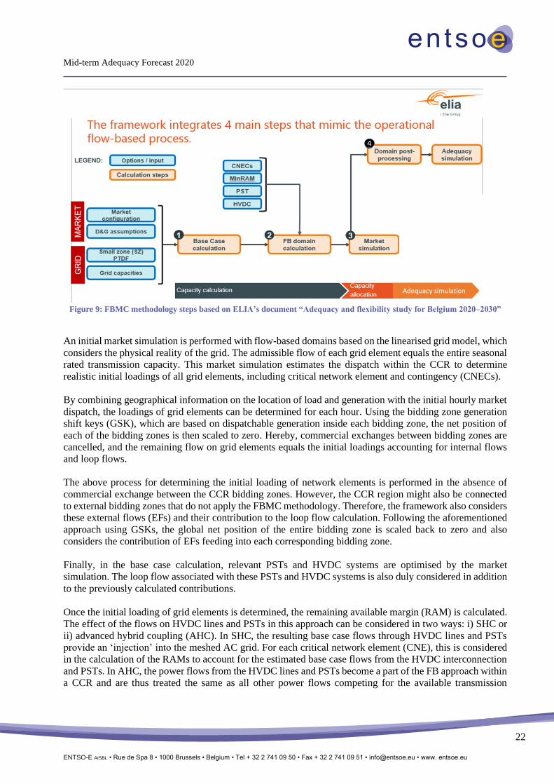
The general FBMC approach has been implemented by the Belgian TSO ELIA16 based on the grid model of
the Ten-Year Network Development Plan (TYNDP) for which flow-based models were developed for the
years 2020, 2023, 2025, 2028 and 2030. This approach is described in the steps illustrated in Figure 9.
16 “Adequacy and flexibility study for Belgium 2020–2030”,
https://www.elia.be/en/news/press-releases/2019/06/20190628_press-release-adequacy-and-flexibility-study-for-
belgium-2020-2030.
Mid-term Adequacy Forecast 2020
ENTSO-E AISBL • Rue de Spa 8 • 1000 Brussels • Belgium • Tel + 32 2 741 09 50 • Fax + 32 2 741 09 51 • [email protected] • www. entsoe.eu
22
Figure 9: FBMC methodology steps based on ELIA’s document “Adequacy and flexibility study for Belgium 2020–2030”
An initial market simulation is performed with flow-based domains based on the linearised grid model, which
considers the physical reality of the grid. The admissible flow of each grid element equals the entire seasonal
rated transmission capacity. This market simulation estimates the dispatch within the CCR to determine
realistic initial loadings of all grid elements, including critical network element and contingency (CNECs).
By combining geographical information on the location of load and generation with the initial hourly market
dispatch, the loadings of grid elements can be determined for each hour. Using the bidding zone generation
shift keys (GSK), which are based on dispatchable generation inside each bidding zone, the net position of
each of the bidding zones is then scaled to zero. Hereby, commercial exchanges between bidding zones are
cancelled, and the remaining flow on grid elements equals the initial loadings accounting for internal flows
and loop flows.
The above process for determining the initial loading of network elements is performed in the absence of
commercial exchange between the CCR bidding zones. However, the CCR region might also be connected
to external bidding zones that do not apply the FBMC methodology. Therefore, the framework also considers
these external flows (EFs) and their contribution to the loop flow calculation. Following the aforementioned
approach using GSKs, the global net position of the entire bidding zone is scaled back to zero and also
considers the contribution of EFs feeding into each corresponding bidding zone.
Finally, in the base case calculation, relevant PSTs and HVDC systems are optimised by the market
simulation. The loop flow associated with these PSTs and HVDC systems is also duly considered in addition
to the previously calculated contributions.
Once the initial loading of grid elements is determined, the remaining available margin (RAM) is calculated.
The effect of the flows on HVDC lines and PSTs in this approach can be considered in two ways: i) SHC or
ii) advanced hybrid coupling (AHC). In SHC, the resulting base case flows through HVDC lines and PSTs
provide an ‘injection’ into the meshed AC grid. For each critical network element (CNE), this is considered
in the calculation of the RAMs to account for the estimated base case flows from the HVDC interconnection
and PSTs. In AHC, the power flows from the HVDC lines and PSTs become a part of the FB approach within
a CCR and are thus treated the same as all other power flows competing for the available transmission

Mid-term Adequacy Forecast 2020
ENTSO-E AISBL • Rue de Spa 8 • 1000 Brussels • Belgium • Tel + 32 2 741 09 50 • Fax + 32 2 741 09 51 • [email protected] • www. entsoe.eu
23
capacity of the AC meshed grid. Therefore, the RAM for the affected CNEs in the AC transmission grid is
not further reduced by the HVDC and/or PST base case power (loop -) flow contribution, as in SHC.
Furthermore, in line with the CEP target for 2025, a minimum margin for trade is applied to the RAM
calculation of each grid element determining the flow-based domains. Notably, this value is 70% for 2025
onwards. Since the initial market simulation has an hourly resolution, it would result in 8760 flow-based
domains for a year. To obtain feasible computation times, a clustering algorithm based on the geometrical
shape of the domains is thus applied, resulting in a specified number of clusters. Next, a representative domain
is selected for each clustered set to be used in the FBMC model. In the final step, a correlation analysis
between the domain clusters and several input parameters is applied to link a given market situation to the
FB domain to be applied. Currently, the selection of German wind infeed and French demand are chosen for
this proof of concept in MAF 2020 as the most relevant parameters in determining the selection of the domain.
This choice is being assessed with respect to the extended geographical scope foreseen from CWE to the
Core region. In any case, the principle remains the same: the hourly choice of the applied domain is based on
the correlation with relevant external parameters and climate variables.
4.2.1.2 Second implementation approach
Another FBMC methodology implementation for the proof of concept in MAF 2020 is based on a
methodology introduced by the French TSO RTE (illustrated in Figure 10). For the initial market simulation,
an NTC approach is chosen. The output of this simulation is then projected on a grid model representing the
expected future grid situation for the time horizon of the study. The result of this step is a nodal model
describing generation, load and power flows for one or multiple time steps. For this nodal model, a remedial
action optimisation is conducted based on a list of CNECs provided for the study. This step ensures that cross-
border exchanges can be maximised. Although this step of the methodology was not performed in the proof
of concept, it is planned to be implemented at a later stage. The next step is then to apply the CWE/core
FBMC methodology to calculate flow-based domains from the CNEC list and the associated remedial actions.
The result is a list of hourly flow-based domains. An optional additional step involves introducing a feedback
loop that delivers the calculated flow-based domains back to the initial market simulation, thereby replacing
the initial NTCs. The process chain can then be re-run for a more robust result. Finally, the set of flow-based
domains resulting from this process can be reduced by geometrical clustering. The clusters are sets of
computed days with a similar shape at hourly resolution. A representative typical day is then selected from
each cluster and can be applied in probabilistic adequacy simulations depending on their correlation with
simulation variables related to adequacy. In this proof of concept, these variables consist of load and power
generation.
Figure 10: RTE FBMC methodology steps.

Mid-term Adequacy Forecast 2020
ENTSO-E AISBL • Rue de Spa 8 • 1000 Brussels • Belgium • Tel + 32 2 741 09 50 • Fax + 32 2 741 09 51 • [email protected] • www. entsoe.eu
24
Preliminary simulations
Based on the two aforementioned FBMC methodology implementations, two sets of FB domains were
provided for probabilistic adequacy studies. The first implementation approach consists of domains prepared
by ELIA, which cover a geographical area very similar to the core CCR, whereas the geographical scope of
the second implementation approach covers the CCR of CWE. For this proof of concept, the first approach
uses domains calculated based on a TYNDP 2018 grid model, whereas the second approach uses domains
obtained from a TYNDP 2020 model. Notably, both sets of domains do not use the same CNEC list since
they were calculated using different grid models. Both domain sets have been implemented for the adequacy
market model of MAF 2019.
The retrieved domains were compared against each other by comparing the vertices in several two-
dimensional representations for CWE countries. This visual comparison showed that even though the two
implementation approaches are different in some respects, the resulting flow-based domains for CWE are
consistent overall.
The two sets of flow-based domains have been integrated into two market simulation tools. Utilising more
than one piece of software helps to validate the simulation results if the outcome for relevant quantities is
aligned. The preliminary results show values for LOLE and EENS that are in the same range for both market
simulation tools. However, certain differences in results are still present and are under investigation.
Conclusions and outlook
FBMC is an established capacity calculation method for inter-zonal trade in the European energy market for
electricity in the CWE region. With its introduction in core CCR, the method becomes even more relevant to
the entire European market and demands a proper representation in mid- and long-term studies. Therefore,
FBMC is planned to be included in the ERAA starting in 2021. As a preparational step, an internal proof of
concept has been performed and reported here in MAF 2020 for information. This proof of concept has
introduced two implementations of the general FBMC methodology that apply to mid- and long-term studies.
While the practical implementations differ on certain points, the resulting FB domains were sufficiently
consistent and affirm the validity of the chosen approaches. The work performed within this ENTSO-E proof
of concept will thus provide the basis for the implementation of FBMC within the ERAA.
For the next steps, the two developed tool chains for domain calculation will be adapted to capture the entire
Core as a CCR. As part of this development, updated market and grid model databases will also be included
in the domain calculations and market simulations. Furthermore, the results of the proof of concept highlight
the importance of considering the effect of curtailment minimisation and curtailment sharing (“adequacy
patch”) in the market simulations once the FBMC approach is fully implemented in the ERAA simulations.
Based on the results obtained, it is observed that once scarcity is present in one or several bidding zones,
‘flow factor competition’17 could lead to situations where order curtailment occurs non-intuitively/unfairly.
For example, this could mean that some buyers (order in the market) that are ready to pay any price to import
energy would be rejected while lower buy bids in other bidding areas are selected instead. Two situations
tend to occur prior to the “adequacy patch” being considered: i) ENS can be created for net exporting
countries to identify the lowest ENS for the FB area as a whole; ii) Countries with low ‘flow factors’ are
penalised with ENS to the benefit of countries with high ‘flow factors’, even if all of these countries are
simultaneously at the maximum market price cap. These are the situations that the adequacy patch must
17 If two possible market transactions generate the same welfare, the one having the lowest impact on the scarce
transmission capacity will be selected first within FBMC. This also means that, in order to optimize the use of the grid
and to maximize the market welfare, some buy (demand) bids with higher prices than other buy (demand) bids located
in other bidding zones, might not be selected within the flow-based allocation. This is a well-known and intrinsic
property of flow-based referred to as “flow factor competition”.

Mid-term Adequacy Forecast 2020
ENTSO-E AISBL • Rue de Spa 8 • 1000 Brussels • Belgium • Tel + 32 2 741 09 50 • Fax + 32 2 741 09 51 • [email protected] • www. entsoe.eu
25
mitigate by correcting flow factor competition while being compliant with the principles of capacity
allocation for the ‘single price coupling’ (EUPHEMIA) algorithm.


![Transparency platform FAQ - ENTSO-E documents... · MONTH-AHEAD TOTAL LOAD FORECAST PER BIDDING ZONE [6.1.D] Q: How should we report the forecast when only some days of the week fall](https://img.pdfslide.us/doc/110x75/60aa9b46bb37df37d65c3275/transparency-platform-faq-entso-e-documents-month-ahead-total-load-forecast.jpg)