10/11/2006

Mid-day Meals and School Attendance: Evidence from Rural India

Kausik Chaudhuri,IGIDR, India

and Sugato DasguptaCESP, JNU, India

10/11/2006

BackgroundTwin objective of universalizing primary education and improving the nutritional intake of students in primary classes.The Mid-day Meal Scheme was launched as a centrally sponsored scheme on August 15, 1995.Cooked mid-day meals would be provided to attending students during lunch break in every government and government-aided primary schools in India within two years.The Supreme Court of India passed a judgment on November 28, 2001 that converted the mid-day meal scheme into a legal entitlement.

10/11/2006

Background

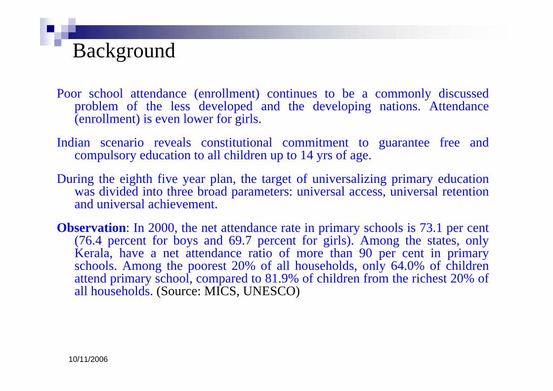
Poor school attendance (enrollment) continues to be a commonly discussed problem of the less developed and the developing nations. Attendance (enrollment) is even lower for girls.

Indian scenario reveals constitutional commitment to guarantee free and compulsory education to all children up to 14 yrs of age.

During the eighth five year plan, the target of universalizing primary education was divided into three broad parameters: universal access, universal retention and universal achievement.

Observation: In 2000, the net attendance rate in primary schools is 73.1 per cent (76.4 percent for boys and 69.7 percent for girls). Among the states, only Kerala, have a net attendance ratio of more than 90 per cent in primary schools. Among the poorest 20% of all households, only 64.0% of children attend primary school, compared to 81.9% of children from the richest 20% of all households. (Source: MICS, UNESCO)

10/11/2006

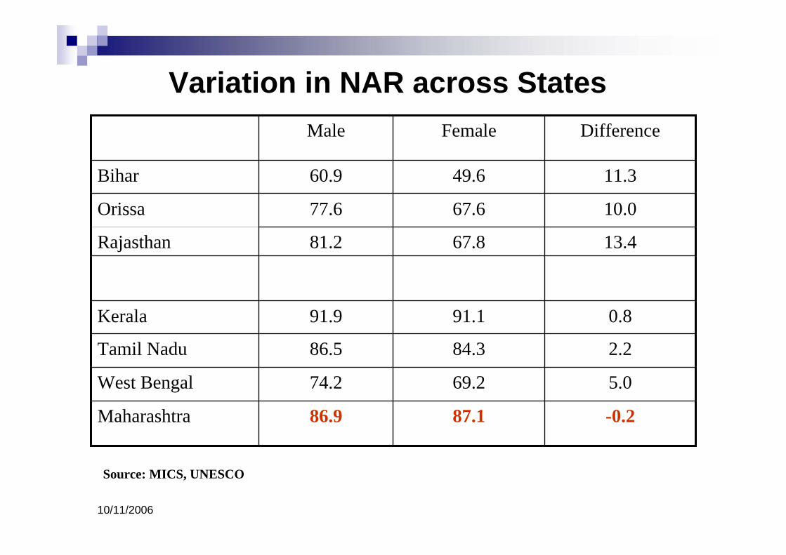
Variation in NAR across States

-0.287.186.9Maharashtra

5.069.274.2West Bengal

2.284.386.5Tamil Nadu

0.891.191.9Kerala

13.467.881.2Rajasthan

10.067.677.6Orissa

11.349.660.9Bihar

DifferenceFemaleMale

Source: MICS, UNESCO

10/11/2006

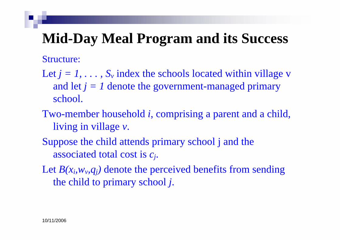
Mid-Day Meal Program and its SuccessStructure:Let j = 1, . . . , Sv index the schools located within village v

and let j = 1 denote the government-managed primary school.

Two-member household i, comprising a parent and a child, living in village v.

Suppose the child attends primary school j and the associated total cost is cj.

Let B(xi,wv,qj) denote the perceived benefits from sending the child to primary school j.

10/11/2006

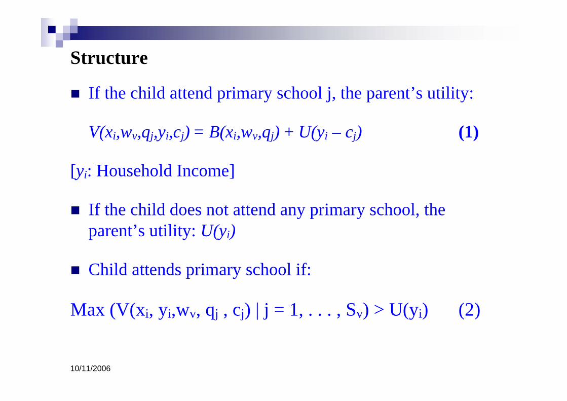
Structure

If the child attend primary school j, the parent’s utility:

V(xi,wv,qj,yi,cj) = B(xi,wv,qj) + U(yi – cj) (1)

[yi: Household Income]

If the child does not attend any primary school, the parent’s utility: U(yi)

Child attends primary school if:

Max (V(xi, yi,wv, qj , cj) | j = 1, . . . , Sv) > U(yi) (2)

10/11/2006

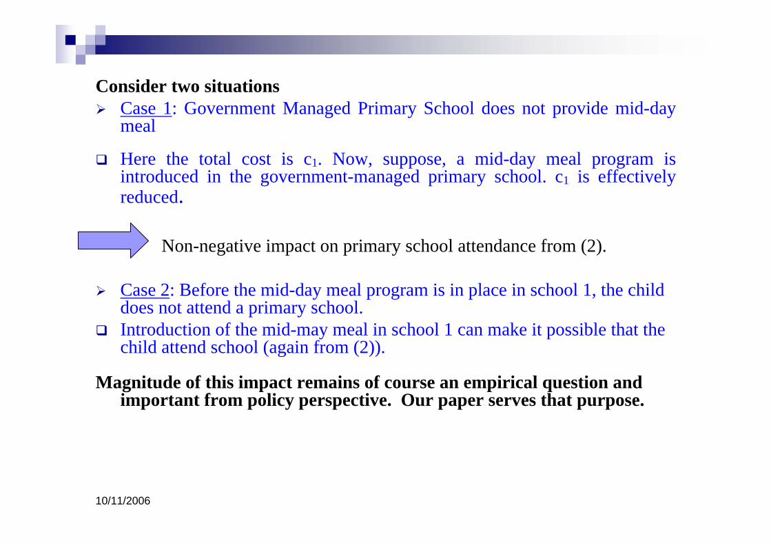
Consider two situationsCase 1: Government Managed Primary School does not provide mid-day meal

Here the total cost is c1. Now, suppose, a mid-day meal program is introduced in the government-managed primary school. c1 is effectively reduced.

Non-negative impact on primary school attendance from (2).

Case 2: Before the mid-day meal program is in place in school 1, the child does not attend a primary school.Introduction of the mid-may meal in school 1 can make it possible that the child attend school (again from (2)).

Magnitude of this impact remains of course an empirical question and important from policy perspective. Our paper serves that purpose.

10/11/2006

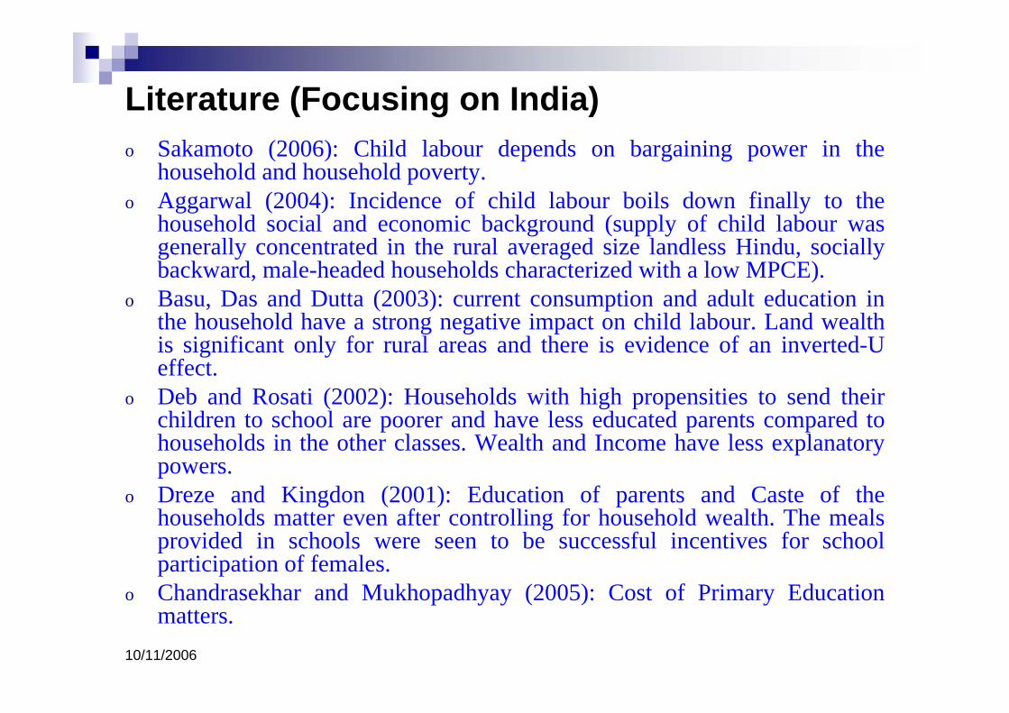
Literature (Focusing on India)o Sakamoto (2006): Child labour depends on bargaining power in the

household and household poverty. o Aggarwal (2004): Incidence of child labour boils down finally to the

household social and economic background (supply of child labour was generally concentrated in the rural averaged size landless Hindu, socially backward, male-headed households characterized with a low MPCE).

o Basu, Das and Dutta (2003): current consumption and adult education in the household have a strong negative impact on child labour. Land wealth is significant only for rural areas and there is evidence of an inverted-U effect.

o Deb and Rosati (2002): Households with high propensities to send their children to school are poorer and have less educated parents compared to households in the other classes. Wealth and Income have less explanatory powers.

o Dreze and Kingdon (2001): Education of parents and Caste of the households matter even after controlling for household wealth. The meals provided in schools were seen to be successful incentives for school participation of females.

o Chandrasekhar and Mukhopadhyay (2005): Cost of Primary Education matters.

10/11/2006

Data

Household data collected by the National Sample Survey Organization, 52nd

round, 1995-96. We use rural data only.

Contains information on the demographic details, and on the educational services received and the educational attainments of persons in the 5-24 years age group.

We focus on 15 major states of India and consider children in the 5-12 years age group.

We address whether primary school attendance affected by access to government-managed primary schools that serve mid-day meals to attending students.

We consider villages if there is a government-managed primary school located within village v.

Our results are unaltered qualitatively under alternative scenario.

10/11/2006

Data (continued)

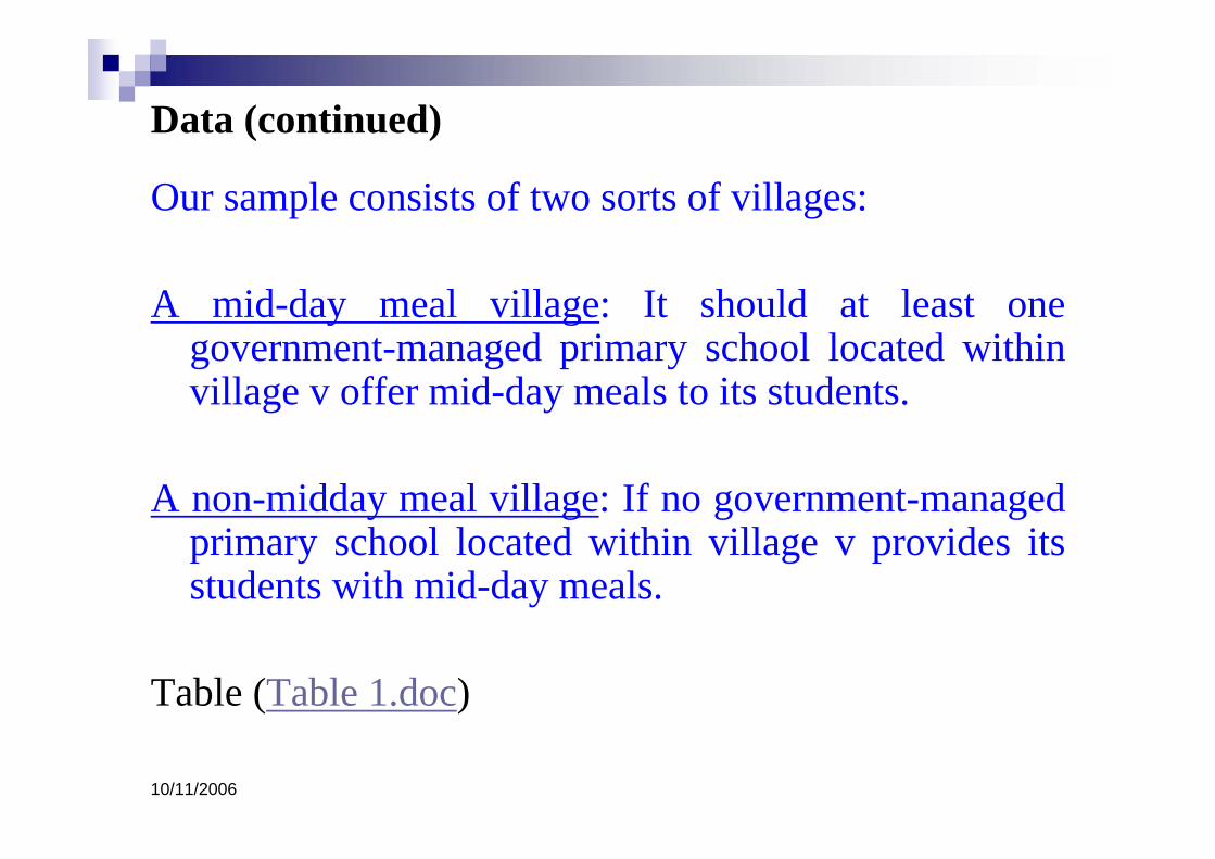
Our sample consists of two sorts of villages:

A mid-day meal village: It should at least one government-managed primary school located within village v offer mid-day meals to its students.

A non-midday meal village: If no government-managed primary school located within village v provides its students with mid-day meals.

Table (Table 1.doc)

10/11/2006

Are primary school attendance rates different across the two village types?

Table 2 provides the answerTable 2.doc

10/11/2006

These differences across the two village types do not imply that the mid-day meal program causally impacts the primary school attendance of children in the targeted age group.

We use Program Evaluation in our case.

10/11/2006

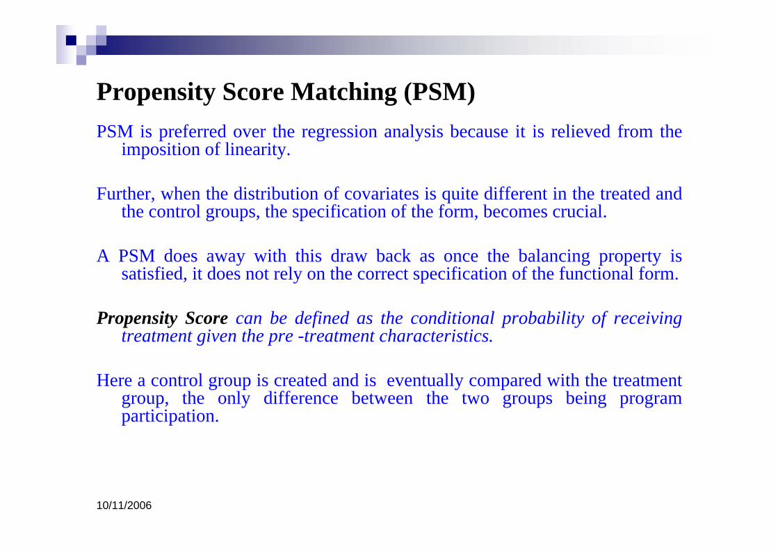
Propensity Score Matching (PSM)PSM is preferred over the regression analysis because it is relieved from the

imposition of linearity.

Further, when the distribution of covariates is quite different in the treated and the control groups, the specification of the form, becomes crucial.

A PSM does away with this draw back as once the balancing property is satisfied, it does not rely on the correct specification of the functional form.

Propensity Score can be defined as the conditional probability of receiving treatment given the pre -treatment characteristics.

Here a control group is created and is eventually compared with the treatment group, the only difference between the two groups being program participation.

10/11/2006

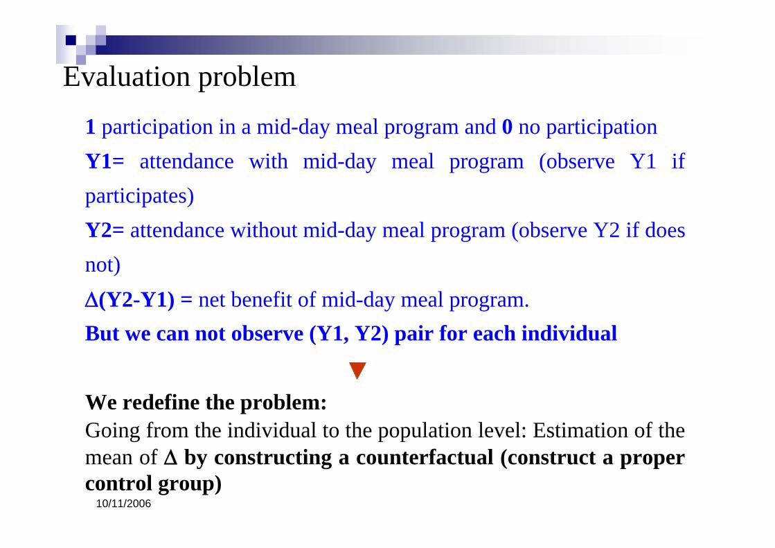
Evaluation problem 1 participation in a mid-day meal program and 0 no participationY1= attendance with mid-day meal program (observe Y1 if participates)Y2= attendance without mid-day meal program (observe Y2 if does not)Δ(Y2-Y1) = net benefit of mid-day meal program.But we can not observe (Y1, Y2) pair for each individual

We redefine the problem:Going from the individual to the population level: Estimation of the mean of Δ by constructing a counterfactual (construct a proper control group)

10/11/2006

Matching

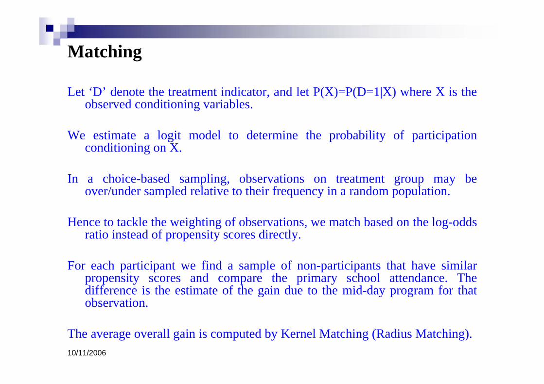
Let ‘D’ denote the treatment indicator, and let P(X)=P(D=1|X) where X is the observed conditioning variables.

We estimate a logit model to determine the probability of participation conditioning on X.

In a choice-based sampling, observations on treatment group may be over/under sampled relative to their frequency in a random population.

Hence to tackle the weighting of observations, we match based on the log-odds ratio instead of propensity scores directly.

For each participant we find a sample of non-participants that have similar propensity scores and compare the primary school attendance. Thedifference is the estimate of the gain due to the mid-day program for that observation.

The average overall gain is computed by Kernel Matching (Radius Matching).

10/11/2006

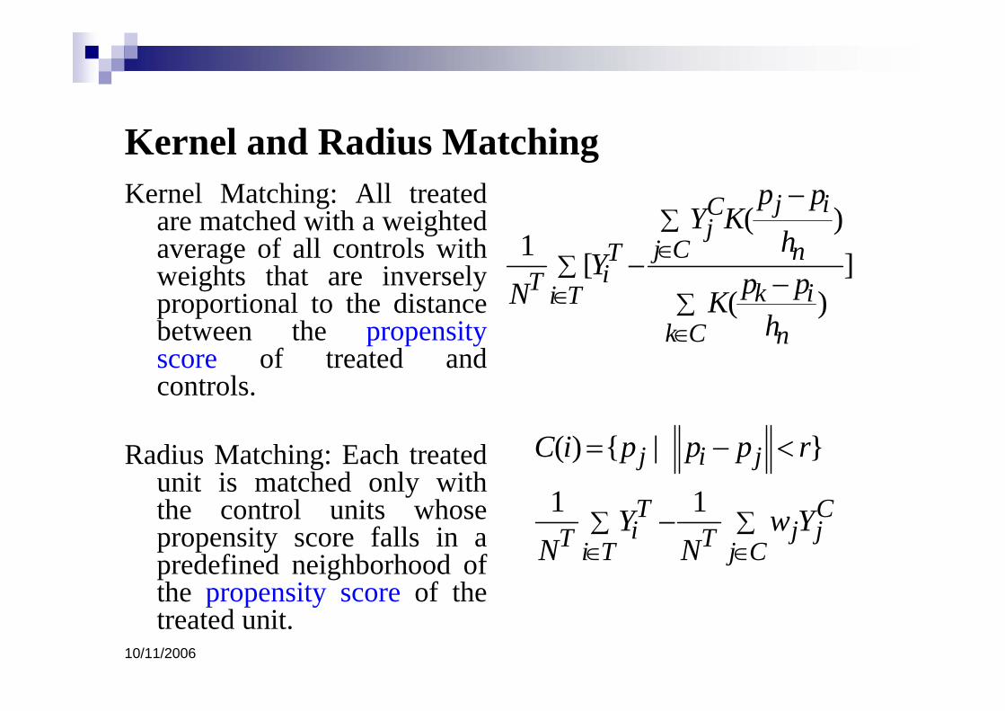
Kernel and Radius MatchingKernel Matching: All treated

are matched with a weighted average of all controls with weights that are inversely proportional to the distance between the propensity score of treated and controls.

Radius Matching: Each treated unit is matched only with the control units whose propensity score falls in a predefined neighborhood of the propensity score of the treated unit.

( )1 [ ]

( )

j iCj

j C nTiT k ii T

k C n

p pY K

hY p pN K

h

∑∈

∑∈ ∑

∈

−

−−

( ) { | }

1 1j i j

T Ci j jT Ti T j C

C i p p p r

Y w YN N

∑ ∑∈ ∈

= − <

−

10/11/2006

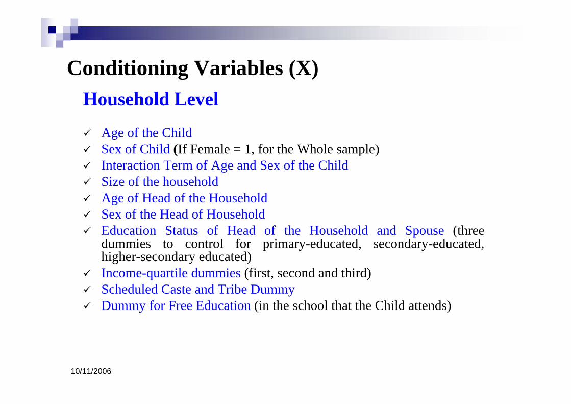
Conditioning Variables (X)Household Level

Age of the ChildSex of Child (If Female = 1, for the Whole sample)Interaction Term of Age and Sex of the ChildSize of the household Age of Head of the Household Sex of the Head of Household Education Status of Head of the Household and Spouse (three dummies to control for primary-educated, secondary-educated, higher-secondary educated)Income-quartile dummies (first, second and third) Scheduled Caste and Tribe DummyDummy for Free Education (in the school that the Child attends)

10/11/2006

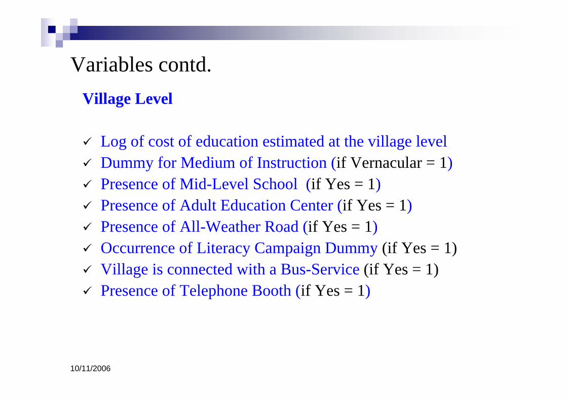
Variables contd.Village Level

Log of cost of education estimated at the village levelDummy for Medium of Instruction (if Vernacular = 1)Presence of Mid-Level School (if Yes = 1)Presence of Adult Education Center (if Yes = 1) Presence of All-Weather Road (if Yes = 1)Occurrence of Literacy Campaign Dummy (if Yes = 1)Village is connected with a Bus-Service (if Yes = 1)Presence of Telephone Booth (if Yes = 1)

10/11/2006

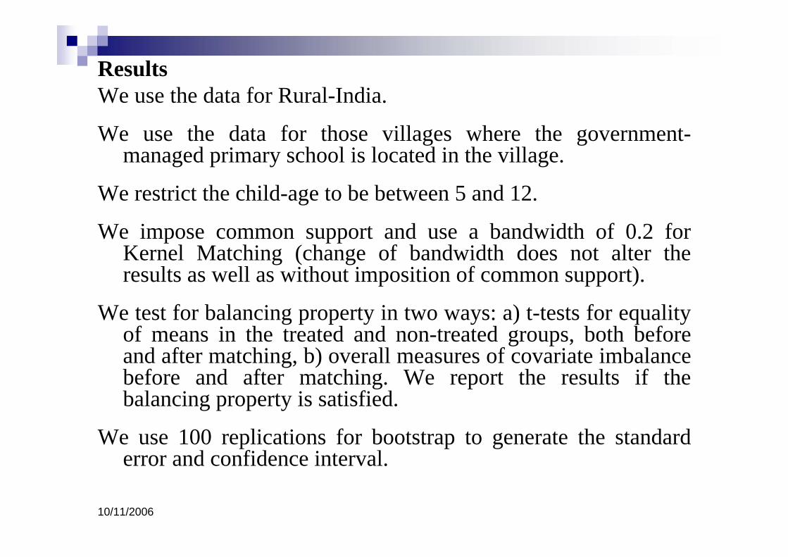
ResultsWe use the data for Rural-India.

We use the data for those villages where the government-managed primary school is located in the village.

We restrict the child-age to be between 5 and 12.

We impose common support and use a bandwidth of 0.2 for Kernel Matching (change of bandwidth does not alter the results as well as without imposition of common support).

We test for balancing property in two ways: a) t-tests for equality of means in the treated and non-treated groups, both before and after matching, b) overall measures of covariate imbalance before and after matching. We report the results if the balancing property is satisfied.

We use 100 replications for bootstrap to generate the standard error and confidence interval.

10/11/2006

Result (Radius Matching)

Table 3.doc

10/11/2006

Result (Kernel Matching)

Table 4.doc

10/11/2006

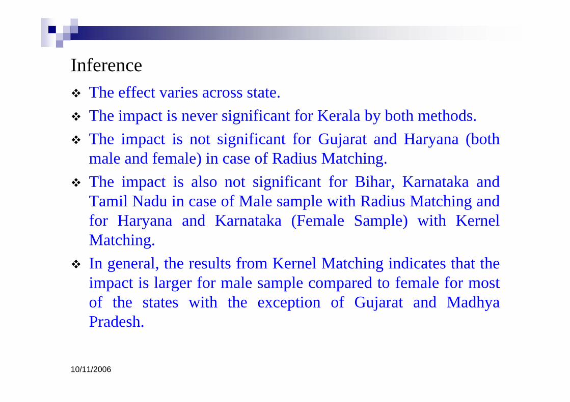
InferenceThe effect varies across state. The impact is never significant for Kerala by both methods.The impact is not significant for Gujarat and Haryana (both male and female) in case of Radius Matching.The impact is also not significant for Bihar, Karnataka and Tamil Nadu in case of Male sample with Radius Matching and for Haryana and Karnataka (Female Sample) with Kernel Matching. In general, the results from Kernel Matching indicates that the impact is larger for male sample compared to female for most of the states with the exception of Gujarat and Madhya Pradesh.

10/11/2006

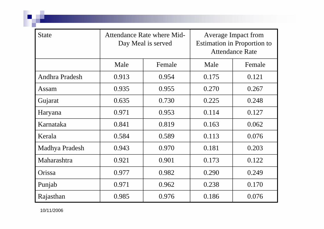
0.2670.2700.9550.935Assam

0.2480.2250.7300.635Gujarat

0.1270.1140.9530.971Haryana

0.0620.1630.8190.841Karnataka

0.186

0.238

0.290

0.173

0.181

0.113

0.175

Male

Average Impact from Estimation in Proportion to

Attendance Rate

0.0760.9760.985Rajasthan

0.1700.9620.971Punjab

0.2490.9820.977Orissa

0.1220.9010.921Maharashtra

0.2030.9700.943Madhya Pradesh

0.0760.5890.584Kerala

0.1210.9540.913Andhra Pradesh

FemaleFemaleMale

Attendance Rate where Mid-Day Meal is served

State

10/11/2006

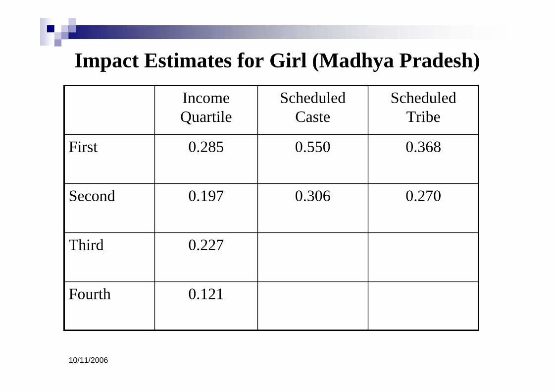
Impact Estimates for Girl (Madhya Pradesh)

0.306

0.550

Scheduled Caste

0.3680.285First

0.121Fourth

0.227Third

0.2700.197Second

Scheduled Tribe

Income Quartile

10/11/2006

ConclusionWe have used the propensity score matching method to quantify the expected gains to children from mid-day meal program, and to examine how those gains vary across Indian States and according to Gender of the Child.

Our method is free from ad-hoc assumptions about the functional for m of impacts and exclusion restrictions. It eliminates selection bias due to observable differences between those having access to mid-day meal program where it is served and those without access.

Results indicate the mid-day meal program increases the attendance rate. This has implications for understanding the incidence of child-education benefits from public policy development program.

Policy makers trying to reach children in poor families—who are typically the most prone to drop-out—will need to do more that relying on making facility placement pro-poor, such as by locating interventions in poor areas.