Embed Size (px)
Citation preview

Microsoft Office Excel 2007
By Paul Stewart Version 2.3/12
2 By P. Stewart Ver. 2.3/12
This tutorial is based on the WordPerfect Suite 6.1 Quattro Pro
tutorial written by Paul Stewart & Gabe Kraljevic 1998
Preface
The notations used in this book are as follows:
-Any text in < > indicates that it is a key on your
keyboard.
e.g. <home>, <1>, <enter>
-press & holding a key <CTRL> + <END> means hold down the
control key <CTRL> and then tap the <END> key, then release the
<CTRL> key.
By P. Stewart Ver. 2.3/12 3
Introduction
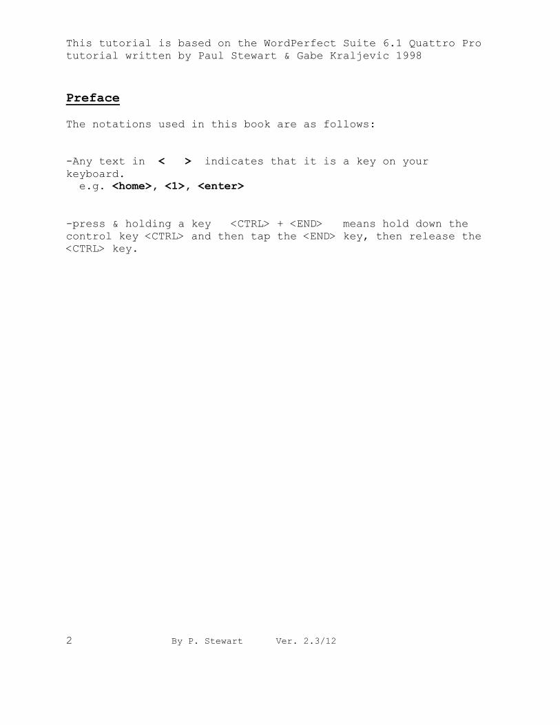
When you start up Microsoft Office Excel 2007 you will see a
screen similar to figure 1.
Figure 1
4 By P. Stewart Ver. 2.3/12
Parts of a Spreadsheet
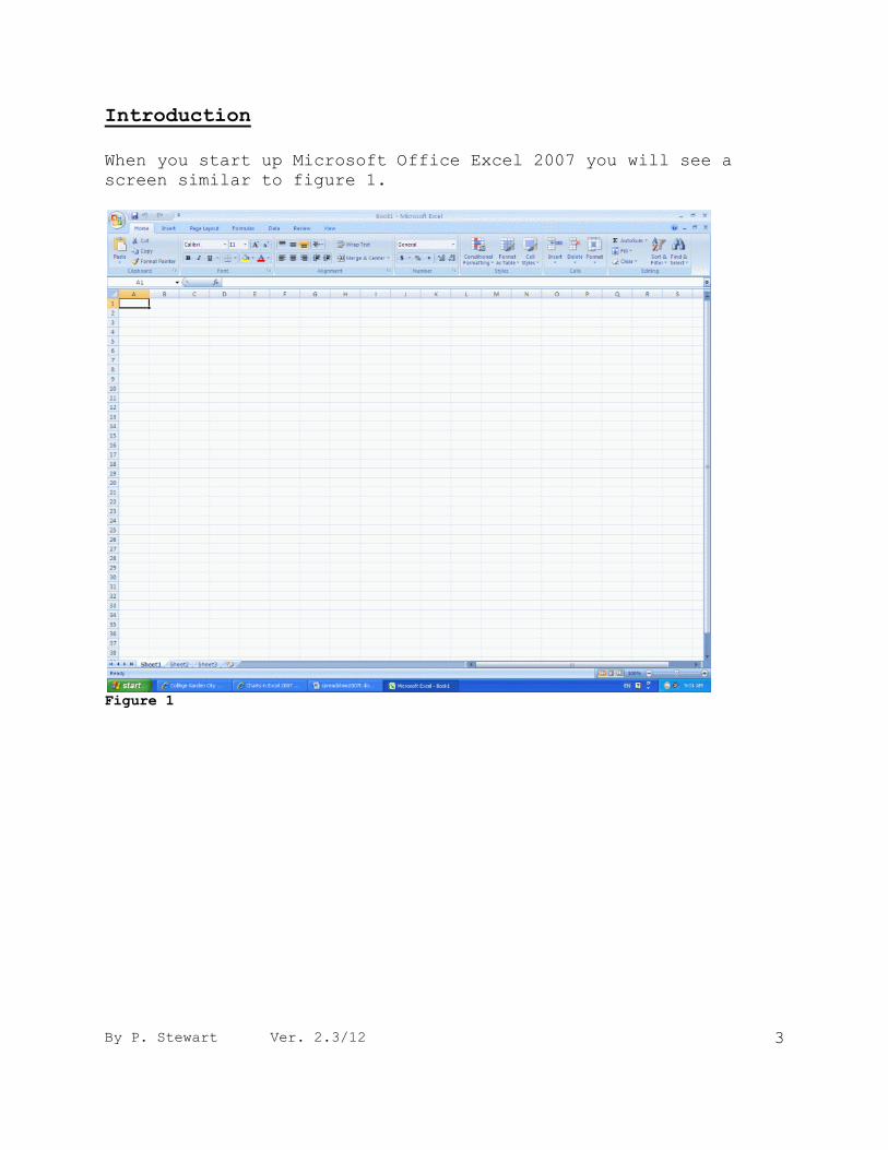
Each spreadsheet is composed of columns and rows for easy
organization of data. The vertical columns in the spreadsheet
are labeled with letters (A, B, C, D, etc.). The numbers on the
left-hand side show the horizontal rows (1, 2, 3, 4,etc.). The
numbers and letters become important in locating the
intersections of rows and columns, which are called cells. A
cell may contain textual data, numerical data or a formula.
Notice that one of the cells is highlighted with a box outline.
The highlighted area is called the cell pointer. This
highlighted area shows that any typing or menu choices will be
entered here. This area is moved around the screen to enter
information.
In the top left of the screen is the cell reference area, this
also indicated the active cell address. This address is the
column letter and row number that is currently highlighted by
the cell pointer.
Just to the right of the cell address the cell contents will be
displayed. Any number, text, or formula that is currently in the
cell will be shown here.
Later in the lessons, you will be introduced to the prompt line
and status line.
By P. Stewart Ver. 2.3/12 5
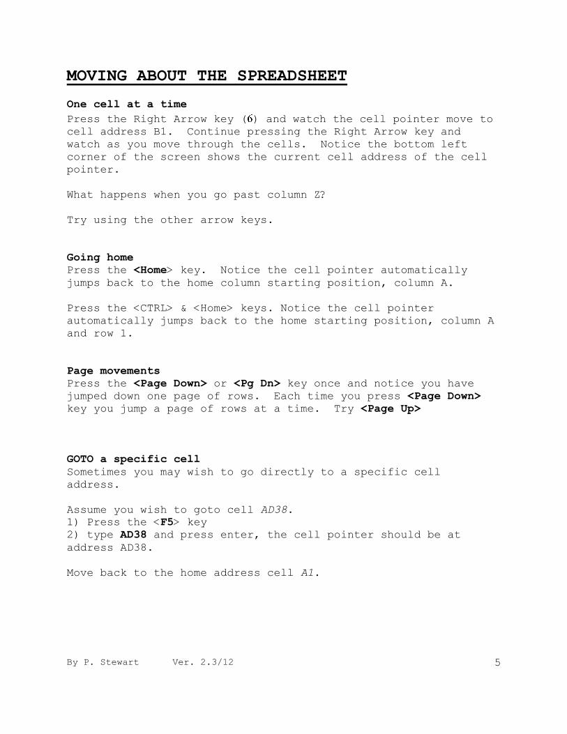
MOVING ABOUT THE SPREADSHEET
One cell at a time
Press the Right Arrow key ( ) and watch the cell pointer move to
cell address B1. Continue pressing the Right Arrow key and
watch as you move through the cells. Notice the bottom left
corner of the screen shows the current cell address of the cell
pointer.
What happens when you go past column Z?
Try using the other arrow keys.
Going home
Press the <Home> key. Notice the cell pointer automatically
jumps back to the home column starting position, column A.
Press the <CTRL> & <Home> keys. Notice the cell pointer
automatically jumps back to the home starting position, column A
and row 1.
Page movements
Press the <Page Down> or <Pg Dn> key once and notice you have
jumped down one page of rows. Each time you press <Page Down>
key you jump a page of rows at a time. Try <Page Up>
GOTO a specific cell
Sometimes you may wish to go directly to a specific cell
address.
Assume you wish to goto cell AD38.
1) Press the <F5> key
2) type AD38 and press enter, the cell pointer should be at
address AD38.
Move back to the home address cell A1.
6 By P. Stewart Ver. 2.3/12
MOUSE movements
Move the mouse pointer to a cell, then click the left mouse
button to move the cursor to that address.
To scroll through the worksheet, click on either the Vertical or
the horizontal scroll bars.
OR
Use the mouse scroll wheel.
ENTERING DATA There are three types of data that can be entered into a
spreadsheet.
1) Labels
Labels are used to describe, comment on, emphasize or highlight
information. Labels are alphanumeric data that includes
numbers, letters and/or other symbols. If you begin an entry
with a letter, the spreadsheet assumes that the entry is a
label.
NOTE: do not start labels with the "=" or A+@ symbol.
If you must use one of these symbols start with a
Quote mark „
2) Values
Values are numerical data. If you begin your entry with a
number, the spreadsheet assumes that entry to be a value.
3) Formulas
Formulas are mathematical or logical expressions that will
calculate numerical values from other cells. A formula is
started with an "@" , “=” or “+” symbol.
Examples of formulas:
FORMULA DESCRIPTION
=SUM(A1.A3) Totals the values of cells A1 + A2 + A3
=AVG(B2.B5) Calculates the average of the cells B2
through B5.
=D8-A4 Subtracts the value in cell A4 from the
value in cell D8.
By P. Stewart Ver. 2.3/12 7
CREATING A SIMPLE BUDGET
You are going to create a simple home budget worksheet. It will
include item categories, budgeted amount, actual amount spent
and the net difference.
(Be sure to begin with a NEW worksheet. )
1. Move the cursor to B2
2. Type HOME BUDGET
You are now going to enter the item categories. As an example
we will have the categories' Groceries, Clothes, Mortgage, etc.
3. Move the cursor to cell A9 and type Groceries
4. Now move to the cell below A10 and type Clothes
5. Type the following categories in the appropriate cells
A11 Mortgage
A12 Electric
A13 Gas
A14 Car
A15 Water
Notice how all the labels automatically align on the left
side, this is called formatting Left Justified.
You are now going to enter the column headings.
6. Move the cursor to A7 and type Item
There are three other columns to label:
Budget, Actual , and Net.
7. Move to cell B7 and type Budget
C7 Actual
D7 Net
You are also going to calculate the Minimum, Maximum and the
Total amount spent.
8 By P. Stewart Ver. 2.3/12
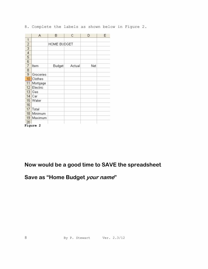
8. Complete the labels as shown below in Figure 2.
Figure 2
Now would be a good time to SAVE the spreadsheet Save as “Home Budget your name”
By P. Stewart Ver. 2.3/12 9
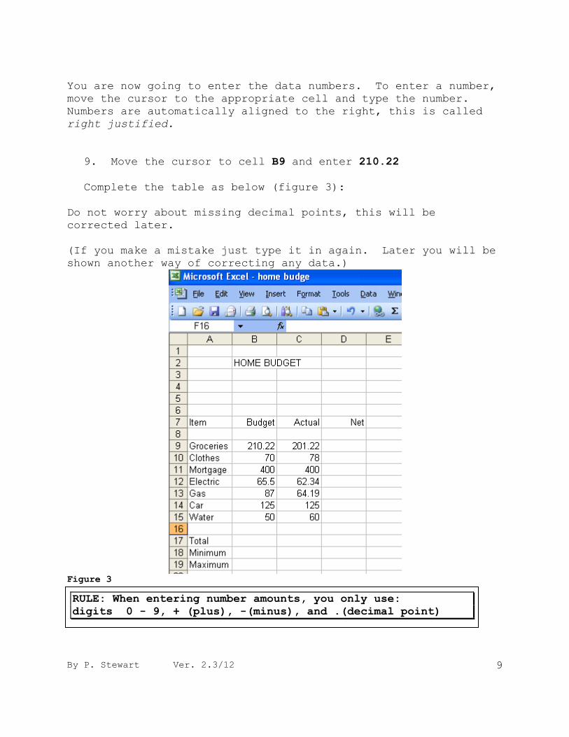
You are now going to enter the data numbers. To enter a number,
move the cursor to the appropriate cell and type the number.
Numbers are automatically aligned to the right, this is called
right justified.
9. Move the cursor to cell B9 and enter 210.22
Complete the table as below (figure 3):
Do not worry about missing decimal points, this will be
corrected later.
(If you make a mistake just type it in again. Later you will be
shown another way of correcting any data.)
Figure 3
RULE: When entering number amounts, you only use:
digits 0 - 9, + (plus), -(minus), and .(decimal point)
10 By P. Stewart Ver. 2.3/12
Entering Formulas
You are now ready to enter the calculations you wish the
worksheet to perform.
To do this you enter formulas in the cell where you wish the
results of the calculations to appear.
In the >Home Budget= we wish to total up the Budget amounts in
cells B9, B10, B11, ... B15 and place this total in cell B17
There are two basic methods of doing this, (Choose either one)
Method One
Enter the formula directly
Move to cell B17, the cell we wish the answer to appear.
Type the formula =SUM(B9.B15) and press <Enter>
Remember, the "=" (equal) sign tells the spreadsheet
program you are entering a formula not a label.
The word SUM is a special function found in the
spreadsheet program. It must be spelled correctly.
The part of the formula, B9.B15, indicates the cells
to sum up. i.e. B9 + B10 + B11 + B12 + B13 + B14 + B15
The formulas do not appear in the cells, but when the cells are
highlighted the formula can be seen in the reference area.
By P. Stewart Ver. 2.3/12 11
Method Two
Using the Auto Sum tool
Highlight the cells to total including the blank location
for the answer.
Highlight Cells B9, B10, B11, to B17
Click the AutoSum tool ∑
AutoSum is found in the Home tab in the Edit Group
The =SUM( ) formula appears in cell B17, this should be the
same as the formula entered above.
Enter an =SUM( ) formula to sum column C (C9 to C15, the answer
in C17)
You decide which method to use.
You are also going to calculate the smallest (minimum) and the
largest (maximum) actual amount spent.
Enter these formulas (remember you must begin the formula by
entering an @ symbol or an = ,equals sign)
C18 =MIN(C9.C15)
C19 =MAX(C9.C15)
You may wish to resave the spreadsheet before you move to the next task. Save as “Home Budget your name”
12 By P. Stewart Ver. 2.3/12
Copying Cells
The last set of formulas to enter will calculate the Net Amount,
or the difference, between the Budgeted Amount (Column B) and
the Actual Amount (Column C). This is calculated by subtracting
Column C from Column B. This needs to be done for all seven
rows; 9 to 15. You do not have to type the formula in seven
times, it can be replicated.
1. Move the cursor to D9.
2. Type the formula +B9-C9
3. With the cursor still on cell D9
-select Copy from the Home tab, clipboard group.
OR
-use the copy quick key <CTRL> & <C>
OR
-use the select Copy from the quick menu (right click
the cell to bring up the quick menu)
3. Highlight the cells we wish to copy the formula to, D10 to D15
With cells highlighted
-select Paste from the Home tab, clipboard group.
OR
-use the Paste quick key <CTRL> & <V>
OR
-use the select Paste from the quick menu (right click
the cell to bring up the quick menu)
The results of the calculations are displayed in the cells that
contained the formulas.
Note: You must begin with the = , + or @ sign. If you do
not the spreadsheet assumes the letter B is the start of a
label, not a formula.
By P. Stewart Ver. 2.3/12 13
FORMATTING
Formatting is the process of changing the appearance of your
spreadsheet to develop a smart looking document. There are
several ways in which you can improve the look of a spreadsheet.
You will notice the headings
BUDGET ACTUAL NET
do not appear over the numbers, they are to the left. To move
these headings to the right you will need to adjust the FORMAT
to right justified.
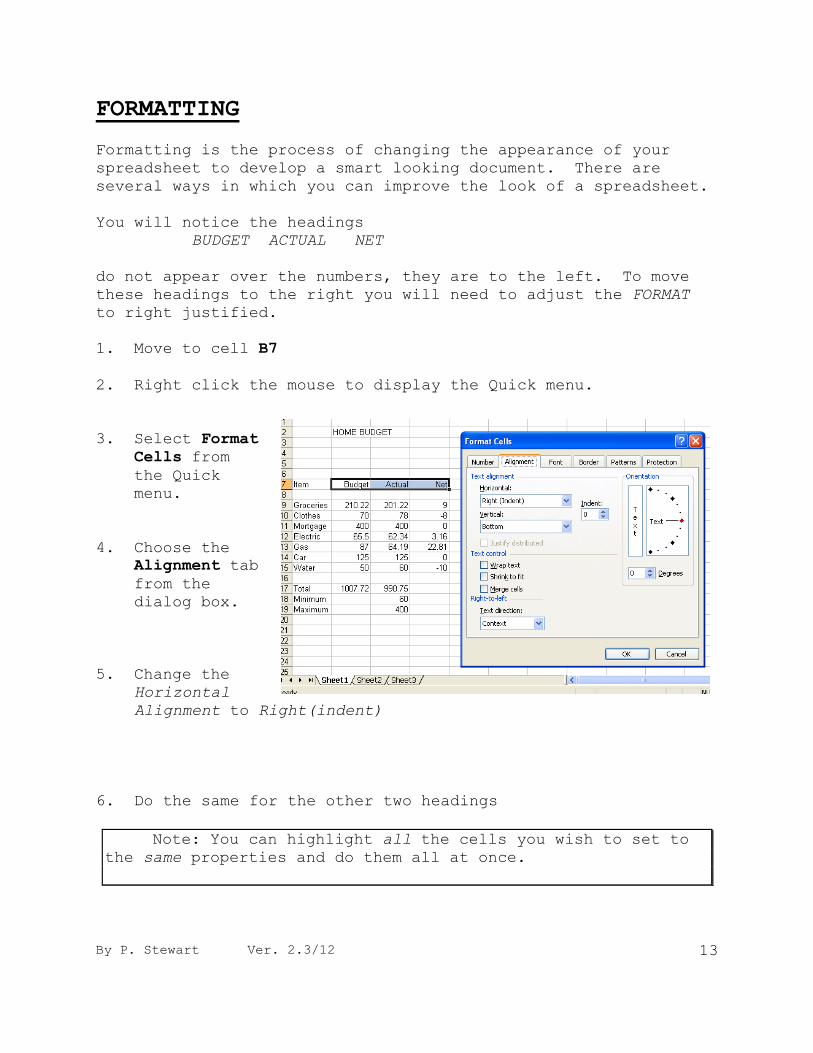
1. Move to cell B7
2. Right click the mouse to display the Quick menu.
3. Select Format
Cells from
the Quick
menu.
4. Choose the
Alignment tab
from the
dialog box.
5. Change the
Horizontal
Alignment to Right(indent)
6. Do the same for the other two headings
Note: You can highlight all the cells you wish to set to
the same properties and do them all at once.
14 By P. Stewart Ver. 2.3/12
You have probably noticed that although the amounts calculated
are dollar amounts, the numbers are not all displayed to two
decimal places. This is because the program does not know we
wish to format the numbers in dollar amounts. This can easily
be changed.
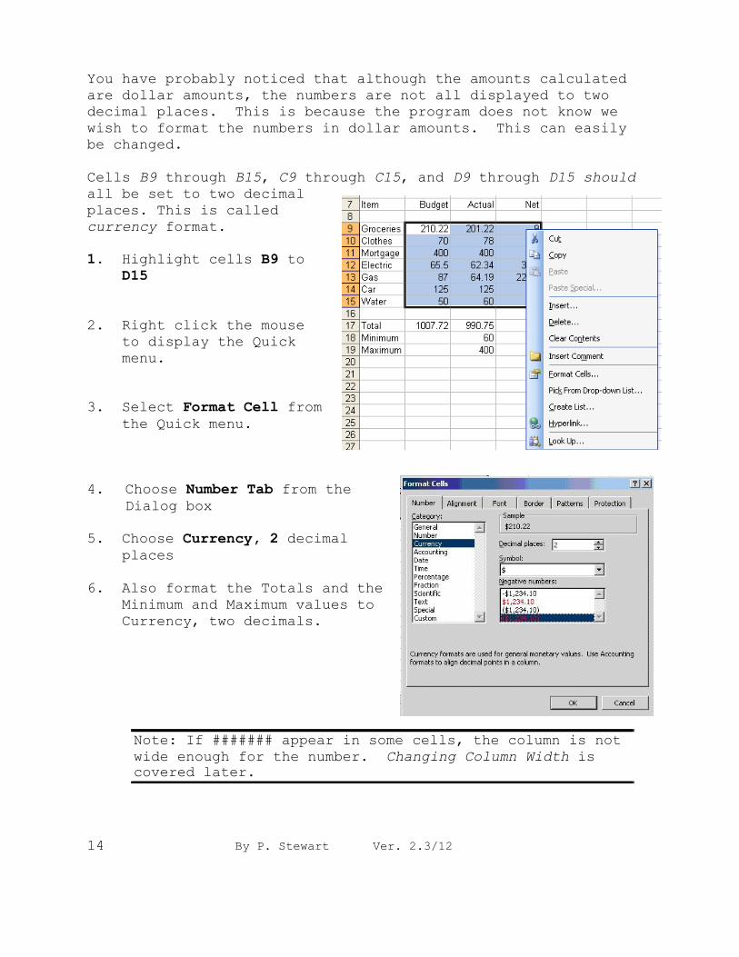
Cells B9 through B15, C9 through C15, and D9 through D15 should
all be set to two decimal
places. This is called
currency format.
1. Highlight cells B9 to
D15
2. Right click the mouse
to display the Quick
menu.
3. Select Format Cell from
the Quick menu.
4. Choose Number Tab from the
Dialog box
5. Choose Currency, 2 decimal
places
6. Also format the Totals and the
Minimum and Maximum values to
Currency, two decimals.
Note: If ####### appear in some cells, the column is not
wide enough for the number. Changing Column Width is
covered later.
By P. Stewart Ver. 2.3/12 15
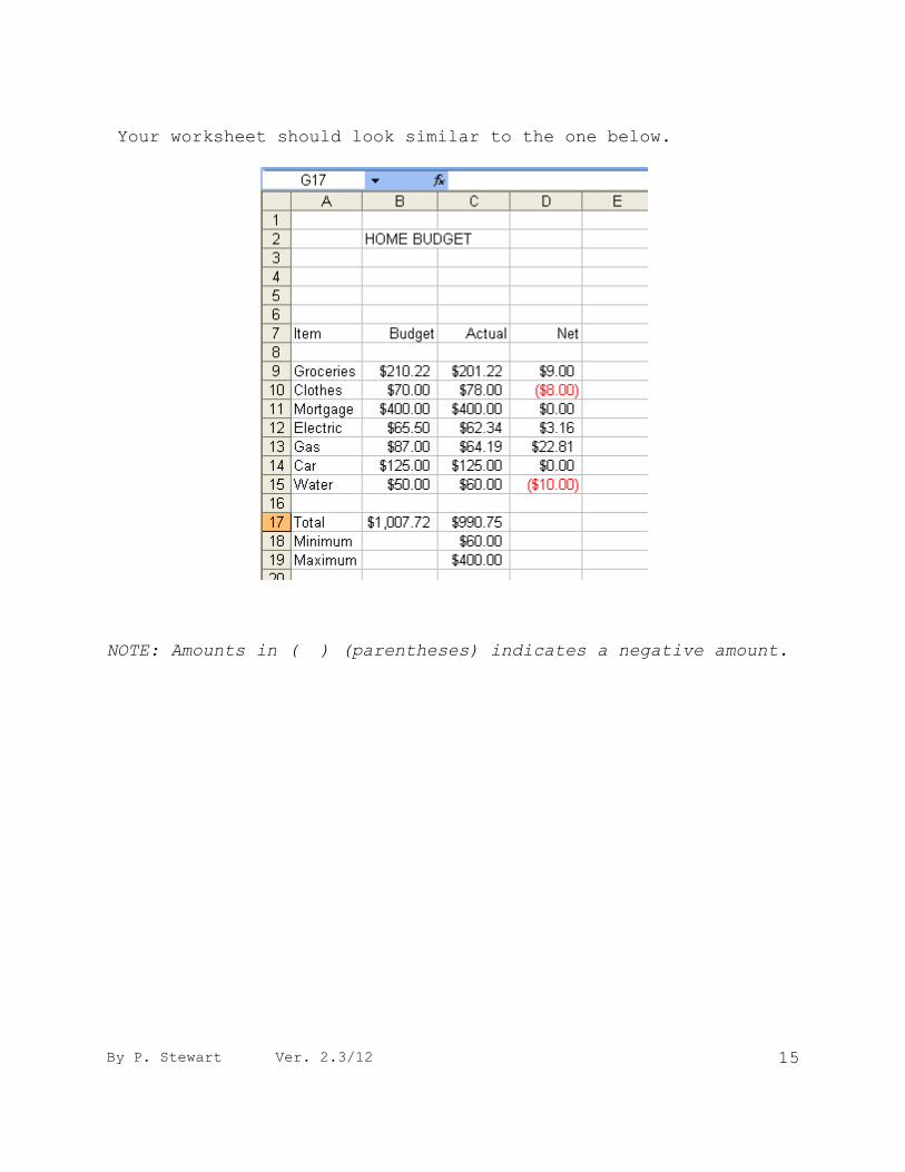
Your worksheet should look similar to the one below.
NOTE: Amounts in ( ) (parentheses) indicates a negative amount.
16 By P. Stewart Ver. 2.3/12
Making Changes & Recalculation
A mistake was made in the ACTUAL AMOUNT spent on ELECTRICITY,
the amount should have been $72.34 NOT $62.34
Changing Values
-Move to cell C12 and type 72.34 and <Enter>
-Notice the amount in cell C12 changed and so did the total in
D12 and C17.
Changing Column Width
If ####### appear in some cells, the column is not wide enough
for the number and you needed to adjust the column width.
-To automatically fit the contents (auto fit)
1. Select the column or columns that you want to change.
2. On the Home tab, in the Cells group, click Format.
3. Under Cell Size, click AutoFit Column Width.
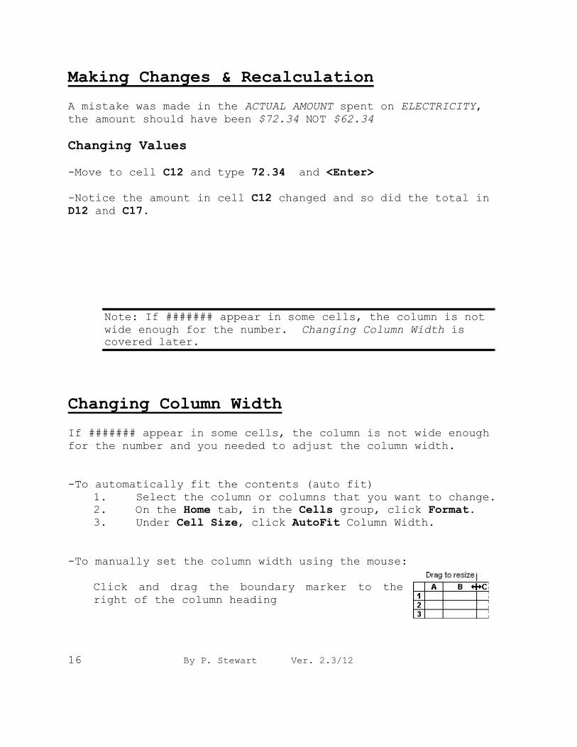
-To manually set the column width using the mouse:
Click and drag the boundary marker to the
right of the column heading
Note: If ####### appear in some cells, the column is not
wide enough for the number. Changing Column Width is
covered later.
By P. Stewart Ver. 2.3/12 17
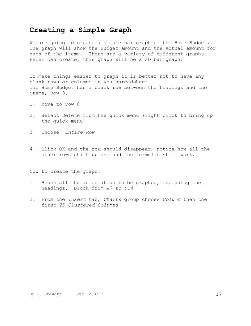
Creating a Simple Graph
We are going to create a simple bar graph of the Home Budget.
The graph will show the Budget amount and the Actual amount for
each of the items. There are a variety of different graphs
Excel can create, this graph will be a 3D bar graph.
To make things easier to graph it is better not to have any
blank rows or columns in you spreadsheet.
The Home Budget has a blank row between the headings and the
items, Row 8.
1. Move to row 8
2. Select Delete from the quick menu (right click to bring up
the quick menu)
3. Choose Entire Row
4. Click OK and the row should disappear, notice how all the
other rows shift up one and the formulas still work.
Now to create the graph.
1. Block all the information to be graphed, including the
headings. Block from A7 to D14
2. From the Insert tab, Charts group choose Column then the
first 2D Clustered Columns
18 By P. Stewart Ver. 2.3/12
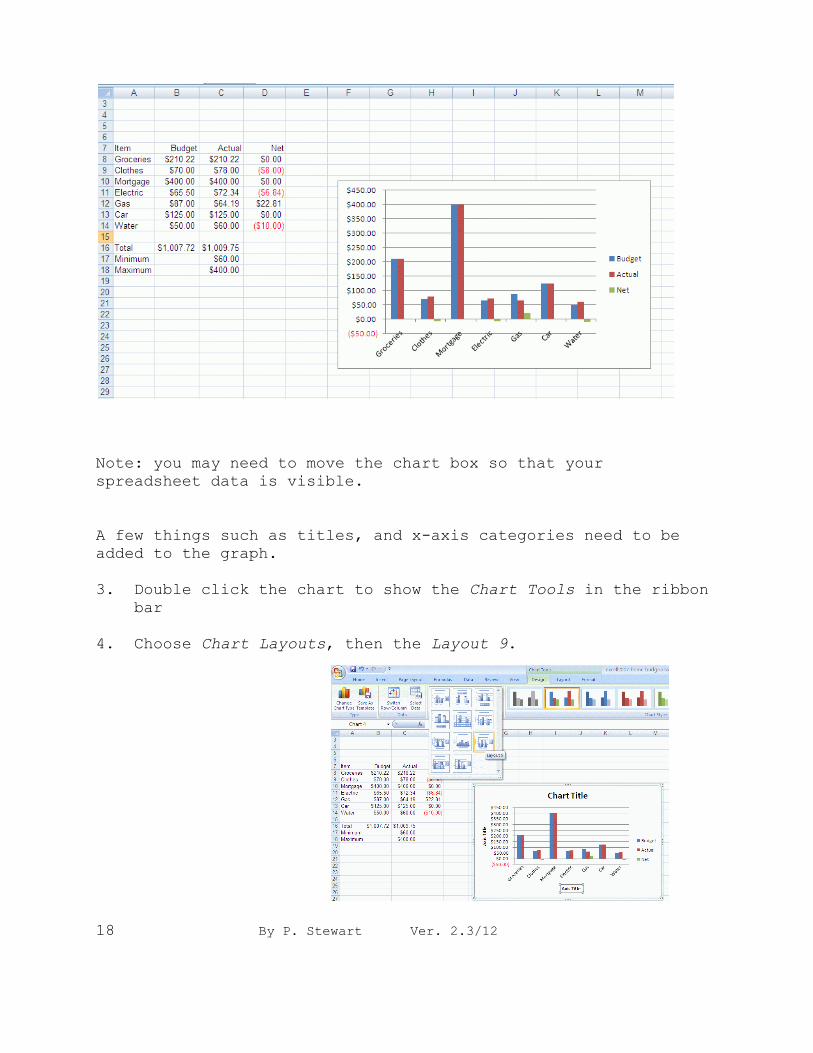
Note: you may need to move the chart box so that your
spreadsheet data is visible.
A few things such as titles, and x-axis categories need to be
added to the graph.
3. Double click the chart to show the Chart Tools in the ribbon
bar
4. Choose Chart Layouts, then the Layout 9.
By P. Stewart Ver. 2.3/12 19
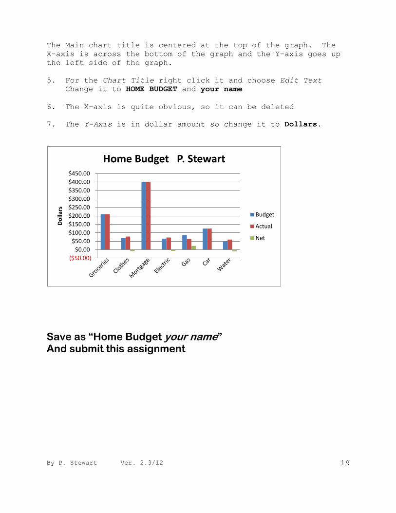
The Main chart title is centered at the top of the graph. The
X-axis is across the bottom of the graph and the Y-axis goes up
the left side of the graph.
5. For the Chart Title right click it and choose Edit Text
Change it to HOME BUDGET and your name
6. The X-axis is quite obvious, so it can be deleted
7. The Y-Axis is in dollar amount so change it to Dollars.
Save as “Home Budget your name” And submit this assignment
($50.00)
$0.00
$50.00
$100.00
$150.00
$200.00
$250.00
$300.00
$350.00
$400.00
$450.00
Do
llars
Home Budget P. Stewart
Budget
Actual
Net
20 By P. Stewart Ver. 2.3/12
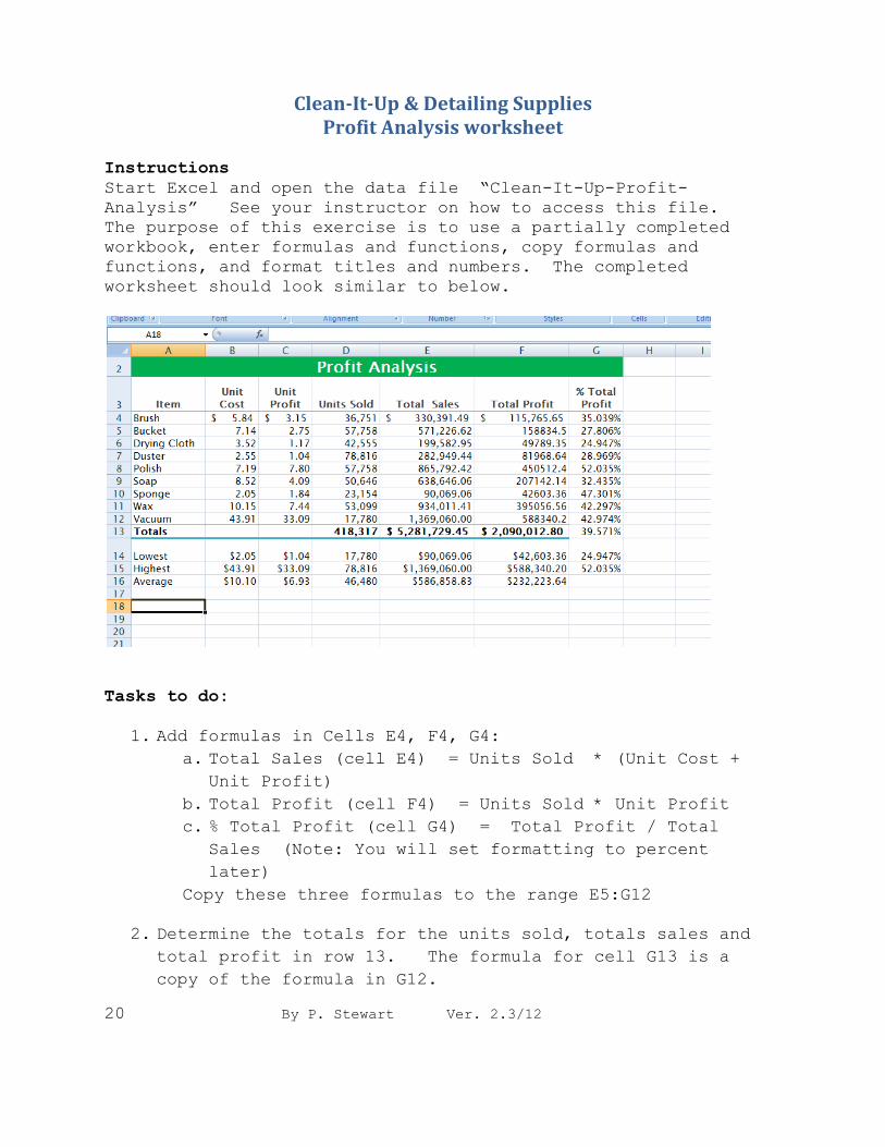
Clean-It-Up & Detailing Supplies Profit Analysis worksheet
Instructions
Start Excel and open the data file “Clean-It-Up-Profit-
Analysis” See your instructor on how to access this file.
The purpose of this exercise is to use a partially completed
workbook, enter formulas and functions, copy formulas and
functions, and format titles and numbers. The completed
worksheet should look similar to below.
Tasks to do:
1. Add formulas in Cells E4, F4, G4:
a. Total Sales (cell E4) = Units Sold * (Unit Cost +
Unit Profit)
b. Total Profit (cell F4) = Units Sold * Unit Profit
c. % Total Profit (cell G4) = Total Profit / Total
Sales (Note: You will set formatting to percent
later)
Copy these three formulas to the range E5:G12
2. Determine the totals for the units sold, totals sales and
total profit in row 13. The formula for cell G13 is a
copy of the formula in G12.
By P. Stewart Ver. 2.3/12 21
3. In the cell range B14:B16, determine the lowest value,
highest value, and average value, for the values in the
range B4:B12. Copy these three functions to the range
C14:G16. Delete the average from cell G16, as an average
of percentages of this type is mathematically invalid
4. Make the following formatting changes
a. Change the workbook theme to Concourse (use the themes
button on the Page layout tab)
b. Cell A1 - change the font size to 24, with a green
background (column 6 of Standard Colors) and white
font colour
c. Cell A2 – change to a green background and white font
colour
d. Cells B4:C4, E4:F4, E13:F13 – Accounting style
formatting with two decimal places
e. Cells B5:C12, E5:F12 - Comma style formatting with
two decimal places
(for Comma -use Number, with 1,000 separator)
f. Cells D4:D16 - Comma style formatting with no decimal
places
g. Cells G4:G15 – Percent style formatting with three
decimal places
h. Cells B14:C16, E14:F16 Currency style formatting with
two decimal places
5. Switch to Page Layout View( View menu, Page Layout) and
enter your name, course, and today‟s date in the header
area. Then change back to Normal View
6. Change the documents properties to include your name and
other pertinent information
7. In Column C, use the keyboard to add manually $1.00 to the
profit for each product with a unit profit of less than
$7.00 and add $3.00 to the profits all other products.
You should end up with $2,765,603.80 in cell F13
8. Save the worksheet as “Clean-It-Up-Profit-Analysis your
name” and submit

22 By P. Stewart Ver. 2.3/12
By P. Stewart Ver. 2.3/12 23
Big Time Lemonade Stand You have gone into an independent business to supplement your income: a
corner lemonade stand (diversified into cookies) which you started 5 days
ago. Being a computer genius, you are going to automate your books.
Now to start the Lemonade Stand finance report.
(Remember to start a New file.)
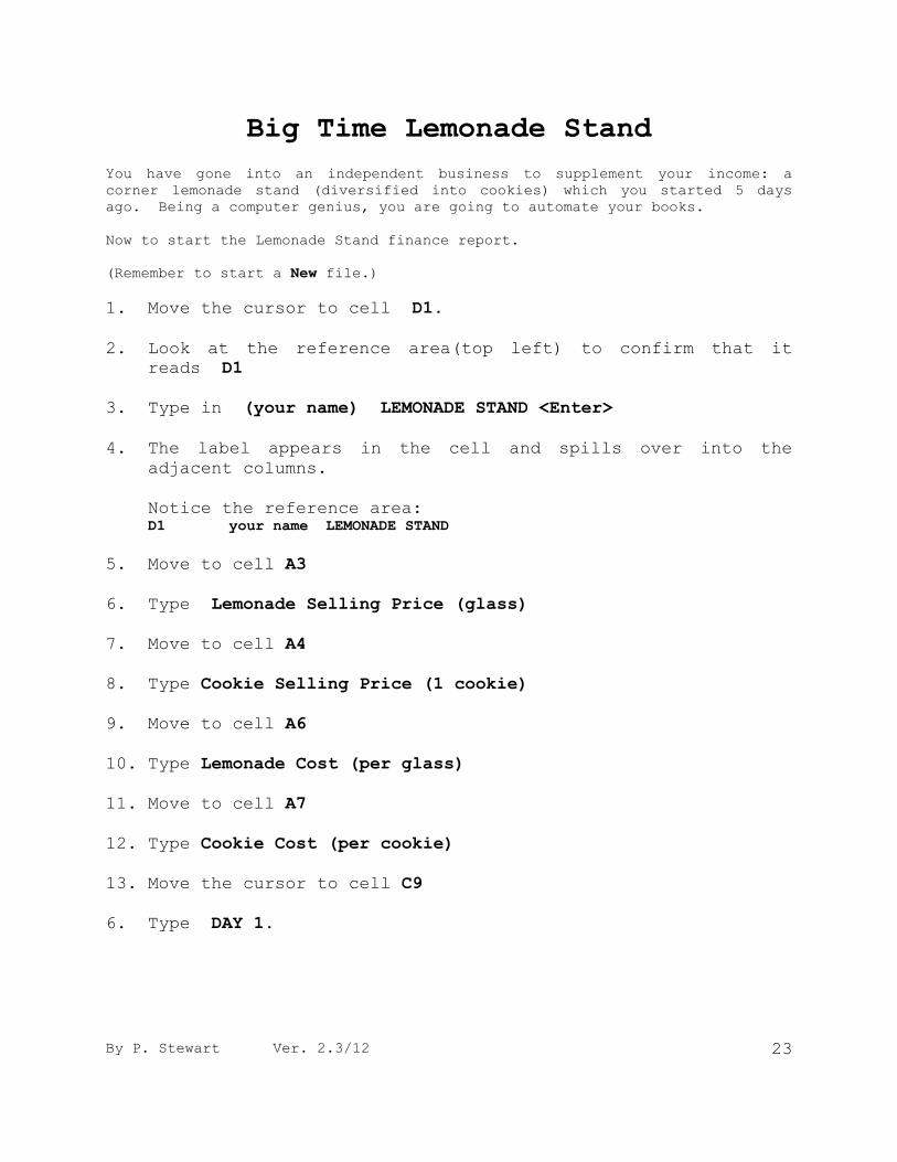
1. Move the cursor to cell D1.
2. Look at the reference area(top left) to confirm that it
reads D1
3. Type in (your name) LEMONADE STAND <Enter>
4. The label appears in the cell and spills over into the
adjacent columns.
Notice the reference area: D1 your name LEMONADE STAND
5. Move to cell A3
6. Type Lemonade Selling Price (glass)
7. Move to cell A4
8. Type Cookie Selling Price (1 cookie)
9. Move to cell A6
10. Type Lemonade Cost (per glass)
11. Move to cell A7
12. Type Cookie Cost (per cookie)
13. Move the cursor to cell C9
6. Type DAY 1.
24 By P. Stewart Ver. 2.3/12
7. Now move to cell D9 and type DAY 2
8. Repeat this so that DAY 3 is in cell E9, DAY 4 in cell
F9 and DAY 5 in cell G9.
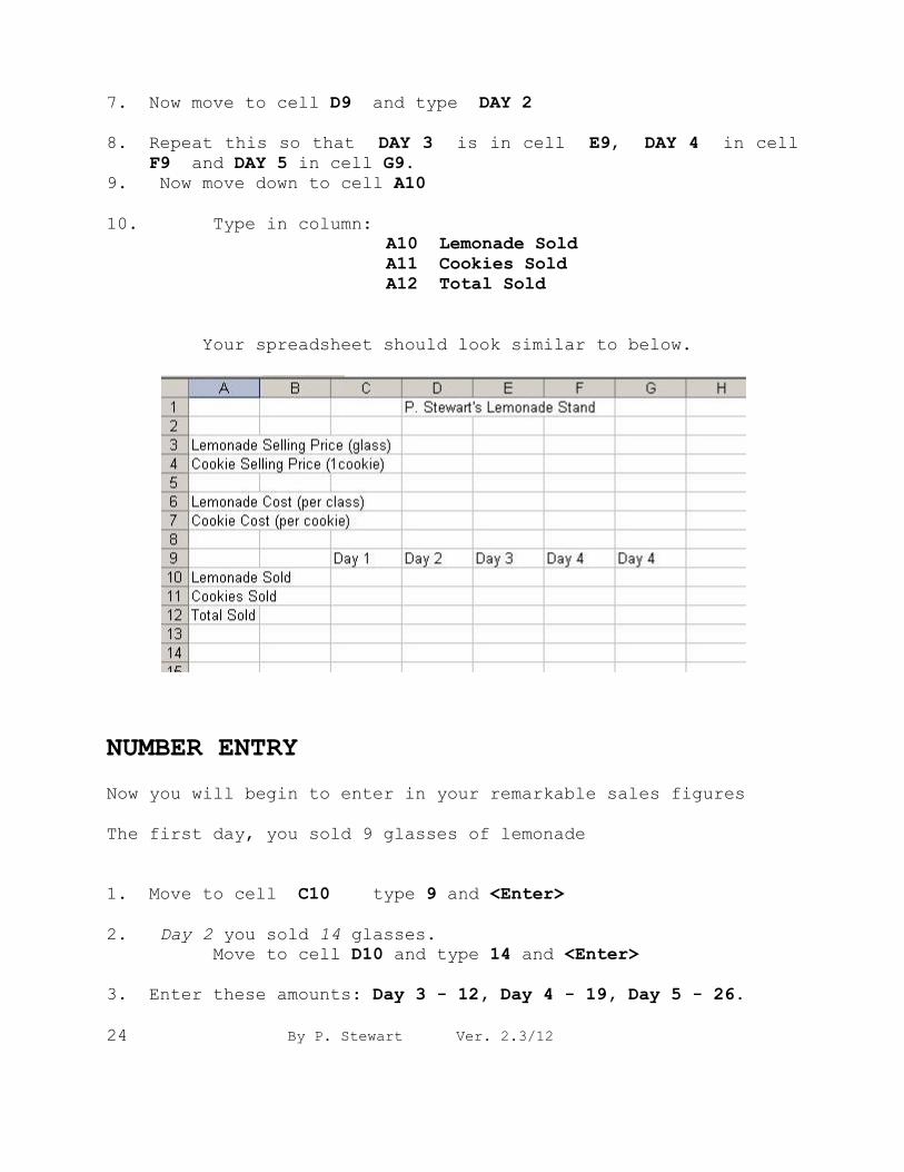
9. Now move down to cell A10
10. Type in column:
A10 Lemonade Sold
A11 Cookies Sold
A12 Total Sold
Your spreadsheet should look similar to below.
NUMBER ENTRY
Now you will begin to enter in your remarkable sales figures
The first day, you sold 9 glasses of lemonade
1. Move to cell C10 type 9 and <Enter>
2. Day 2 you sold 14 glasses.
Move to cell D10 and type 14 and <Enter>
3. Enter these amounts: Day 3 - 12, Day 4 - 19, Day 5 - 26.
By P. Stewart Ver. 2.3/12 25
4. Now enter the COOKIE sales data on row 11
DAY 1 - 7, DAY 2 - 16, DAY 3 - 11, DAY 4 - 23, DAY 5 - 24
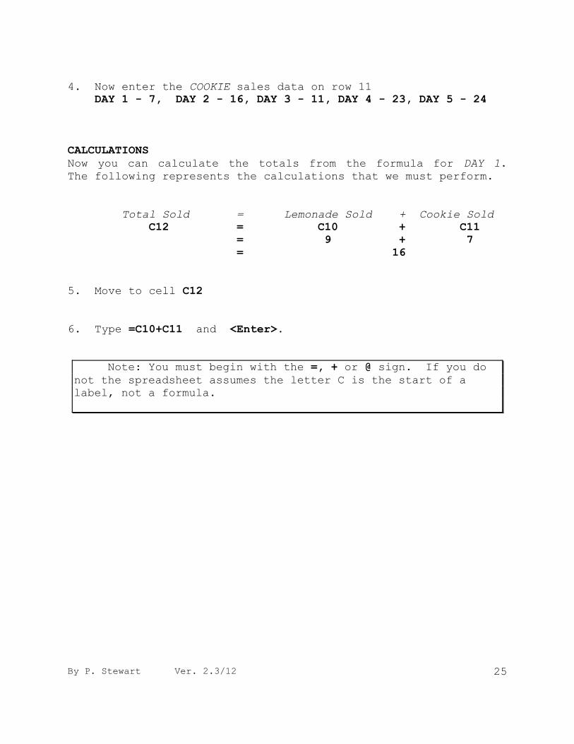
CALCULATIONS
Now you can calculate the totals from the formula for DAY 1.
The following represents the calculations that we must perform.
Total Sold = Lemonade Sold + Cookie Sold
C12 = C10 + C11
= 9 + 7
= 16
5. Move to cell C12
6. Type =C10+C11 and <Enter>.
Note: You must begin with the =, + or @ sign. If you do
not the spreadsheet assumes the letter C is the start of a
label, not a formula.
26 By P. Stewart Ver. 2.3/12
REPLICATION (copying formulas)
To obtain the total sold figure for Days 2 - 5, use the copy and
paste commands to copy the formula in cell C12 to cells D12,
E12, F12 and G12 rather than retyping it four times with
different column letters.
1. Move to the cell to be copied, C12
With the cursor still on cell C12
-select Copy from the Home tab, clipboard group.
OR
-use the copy quick key <CTRL> & <C>
OR
-use the select Copy from the quick menu (right click
the cell to bring up the quick menu)
2. Highlight the cells we wish to copy the formula to
D12 to G12
With cells highlighted
-select Paste from the Home tab, clipboard group.
OR
-use the Paste quick key <CTRL> & <V>
OR
-use the select Paste from the quick menu (right click
the cell to bring up the quick menu)
The results of the calculations are displayed in the cells that
contained the formulas.
Note that the formulas use different cell addresses. The
spreadsheet changes the cell addresses when copying to
reflect the relative positions of cells in the copied
formula.
By P. Stewart Ver. 2.3/12 27
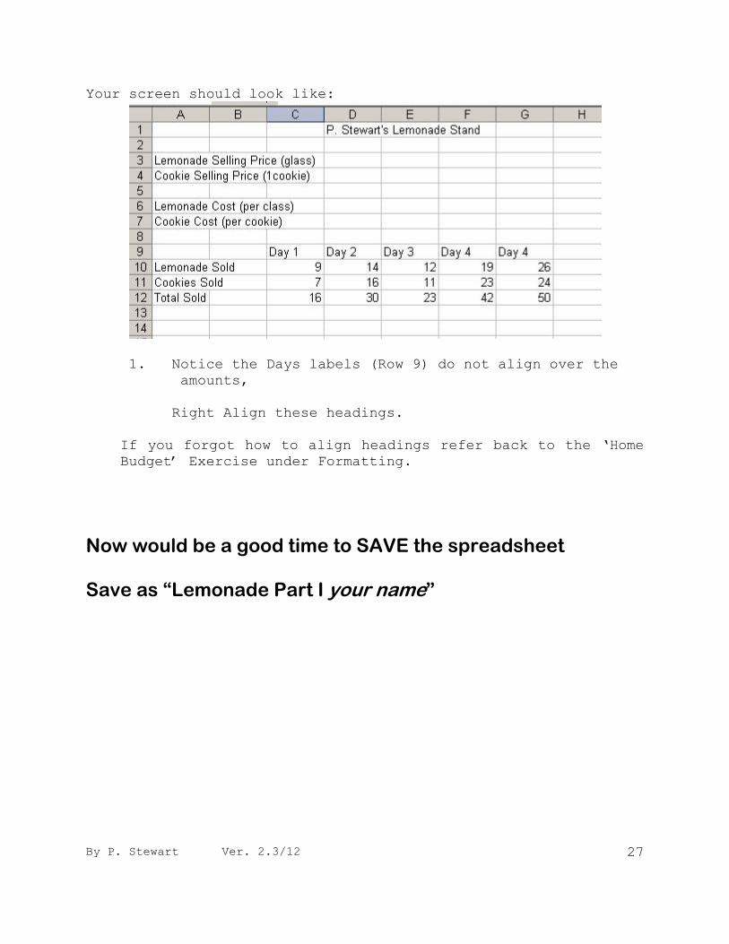
Your screen should look like:
1. Notice the Days labels (Row 9) do not align over the
amounts,
Right Align these headings.
If you forgot how to align headings refer back to the „Home
Budget‟ Exercise under Formatting.
Now would be a good time to SAVE the spreadsheet Save as “Lemonade Part I your name”
28 By P. Stewart Ver. 2.3/12
Calculating the Selling Price (absolute addresses)
To figure out the income from the lemonade stand we need to know
the selling price of our products.
Lemonade is being sold for $0.15 a glass and
Cookies are being sold for $0.35 each.
1. In cell D3 enter the amount for lemonade .15
2. In cell D4 enter the amount for cookies .35
3. In the following cells enter these labels
A14 Lemonade Income
A15 Cookie Income
A16 Gross Income
4. Since the price and the number sold is known, it is easy to
calculate the dollar amount made in sales.
The formula for dollars of sales for lemonade on...
Day 1 is:
Lemonade Income = Price of lemonade * Number sold
C14 = D3 * C10
Day 2 is:
Lemonade Sales = Price of lemonade * Number sold
D14 = D3 * D10
Notice that the cell address for price of lemonade, D3,
must not change.
Move to cell C14 and enter the formula =$D$3 * C10
In spreadsheets the asterisk (*) is used for multiplication; the forward
slash (/) is used for division.
The $ in front of the D and 3 mean absolute address, When the
cell formula is copied to another cell, D3 will not change
(absolute), where C10 should change when the formula is copied.
NOTE: The answer is NOT to two decimal places, this will be

By P. Stewart Ver. 2.3/12 29
corrected later.
30 By P. Stewart Ver. 2.3/12
4. Copy this formula to cells D14 to G14
5. Move to cell C15 and enter the formula for cookie income
=$D$4*C11
6. Copy this formula to cells D15, E15, F15 and G15.
7. Now enter a formula to calculate the Gross Income.
(Lemonade Income + Cookie Income)
Move to cell C16 and enter the formula =C14+C15.
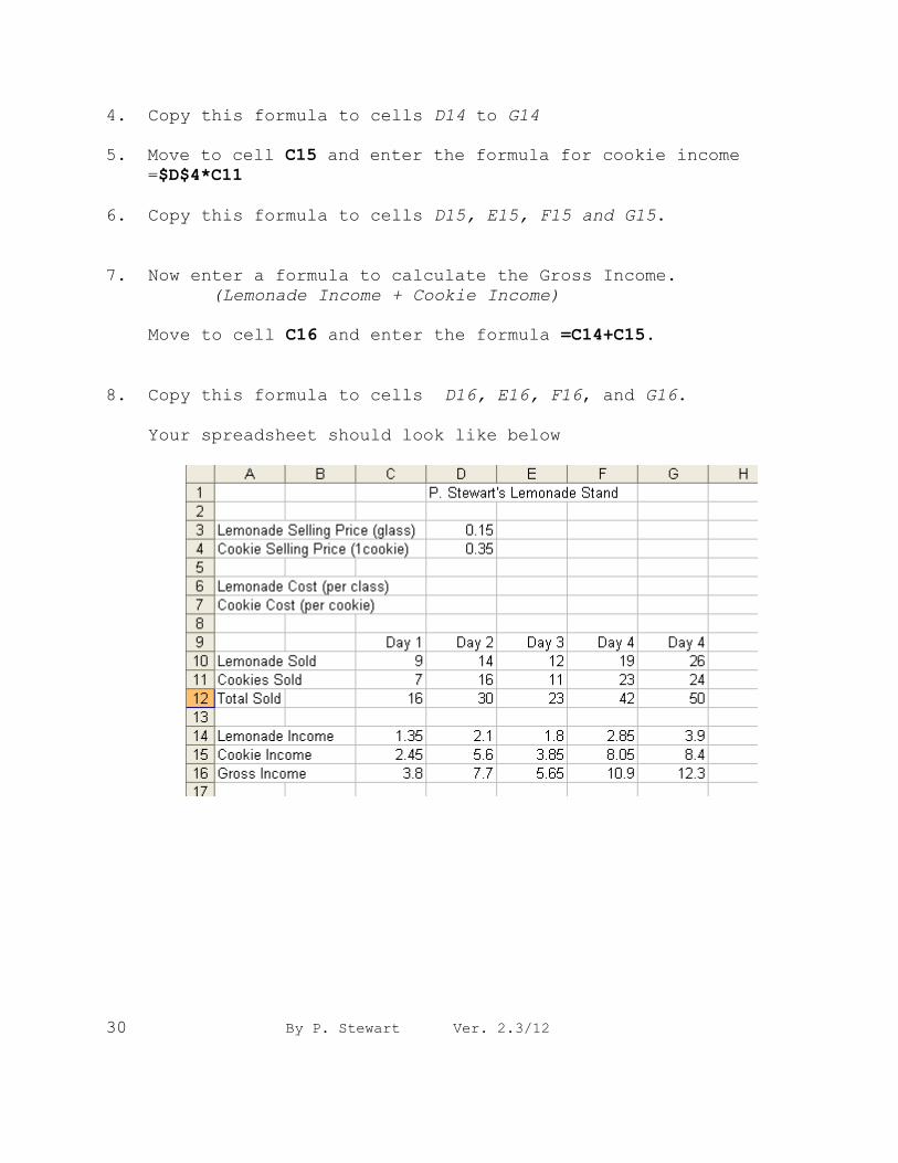
8. Copy this formula to cells D16, E16, F16, and G16.
Your spreadsheet should look like below
By P. Stewart Ver. 2.3/12 31
FORMATTING
You have probably noticed that although the amounts calculated
are dollar amounts, the numbers are not all displayed to two
decimal places. This is because the program does not know the
format we wish to use is for dollar amounts. This can easily be
changed.
Cells C14, D14, E14, F14, G14; C15, D15,...G15; and C16,
D16,...G16 should all be set to two decimal places, Currency,
format.
1. Highlight cells C14 to G16
2. With your cursor on any of these cells choose Format Cells
from the Quick menu
3. Select the Number tab, Currency, two decimals.
4. Format the lemonade & cookie selling price to Currency, 2
decimals. Cells D3 & D4
If you have not already done so, the headings for the Days
should align on the right side of the cell to look better
1. Highlight the headings DAY1, DAY2, etc.
2. With your cursor on any of these cells choose Format Cell
from the Quick menu
3. Select the Alignment tab, change the Text alignment:
Horizontal to Right(indent).
32 By P. Stewart Ver. 2.3/12
Now we need to figure out how much it will cost to produce our
products, so that you can determine the Net Profit made.
1. In the Column D of rows 6 & 7 add the values.
A6 Lemonade Cost (per glass) .03
A7 Cookie Cost (per cookie) .05
2. Add the following new labels
A18 Lemonade Cost
A19 Cookie Cost
A20 Total Cost
A22 Net Profit
3. Now to calculate these costs, it is similar to calculating
the Lemonade & cookie sold.
Absolute addresses must be used.
Day 1 Lemonade cost = Lemonade cost (per glass) * Day 1 Lemonade
Sold
C18 $D$6 * C10
The lemonade cost D6 never changes so it is an absolute address
In cell C18 enter the formula =$D$6*C10
4. Copy this formula to the cells D18, E18, F18, G18
5. Enter a similar formula for Cookie cost, and copy it as
needed.
6. The Total Cost is calculated by adding Lemonade Cost and
Cookie Cost , enter this formula and copy it.
7. The Net Profit is calculated by Gross Income - Total Cost,
enter this formula and copy it.
8. Format these amounts to Currency, two decimals
By P. Stewart Ver. 2.3/12 33
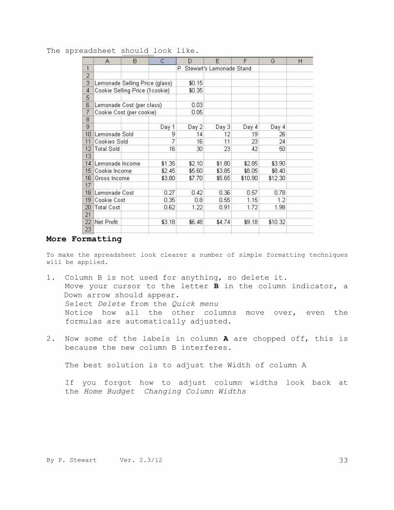
The spreadsheet should look like.
More Formatting
To make the spreadsheet look clearer a number of simple formatting techniques
will be applied.
1. Column B is not used for anything, so delete it.
Move your cursor to the letter B in the column indicator, a
Down arrow should appear.
Select Delete from the Quick menu
Notice how all the other columns move over, even the
formulas are automatically adjusted.
2. Now some of the labels in column A are chopped off, this is
because the new column B interferes.
The best solution is to adjust the Width of column A
If you forgot how to adjust column widths look back at
the Home Budget Changing Column Widths
34 By P. Stewart Ver. 2.3/12
When entering Currency amounts, standard accounting procedure is
to only put the Dollar sign on the total row, not on every row
as has been done in the Lemonade Stand. The non-total rows
should have two decimals but not the dollar sign.
3. Highlight the Lemonade Income and Cookie Income amounts
(cells B14 to F15).
Change the Numeric Format to Number, 2 decimals ,
Use 1000 separator.
4. Do the same for the Lemonade Cost and Cookie Cost (cells B18
to F19)
5. Highlight the DAY headings, and choose Format Cell from the
Quick menu
6. Choose Font, and change the Point Size to 14, and Bold.
7. Do the same to the heading at the top (your name Lemonade
Stand)
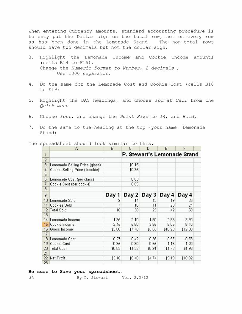
The spreadsheet should look similar to this.
Be sure to Save your spreadsheet.
By P. Stewart Ver. 2.3/12 35
GRAPHING
Now that the first week is well under way, it is time to
franchise. But, the prospective franchise buyer must be
convinced of the profit possible. What better method than to
use a graph.
A graph will be created showing the lemonade and cookie income
for each day.
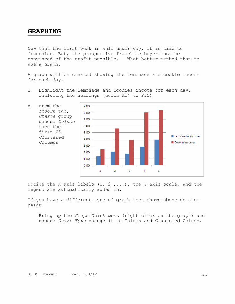
1. Highlight the lemonade and Cookies income for each day,
including the headings (cells A14 to F15)
8. From the
Insert tab,
Charts group
choose Column
then the
first 2D
Clustered
Columns
Notice the X-axis labels (1, 2 ,...), the Y-axis scale, and the
legend are automatically added in.
If you have a different type of graph then shown above do step
below.
Bring up the Graph Quick menu (right click on the graph) and
choose Chart Type change it to Column and Clustered Column.
36 By P. Stewart Ver. 2.3/12
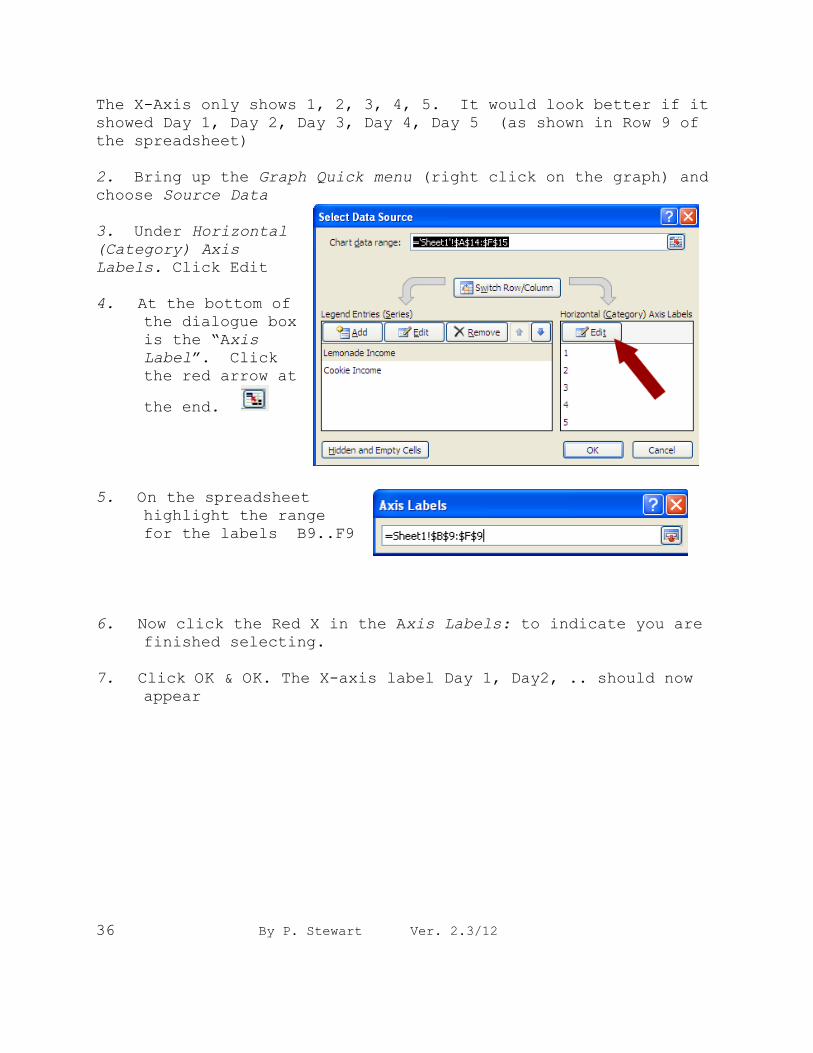
The X-Axis only shows 1, 2, 3, 4, 5. It would look better if it
showed Day 1, Day 2, Day 3, Day 4, Day 5 (as shown in Row 9 of
the spreadsheet)
2. Bring up the Graph Quick menu (right click on the graph) and
choose Source Data
3. Under Horizontal
(Category) Axis
Labels. Click Edit
4. At the bottom of
the dialogue box
is the “Axis
Label”. Click
the red arrow at
the end.
5. On the spreadsheet
highlight the range
for the labels B9..F9
6. Now click the Red X in the Axis Labels: to indicate you are
finished selecting.
7. Click OK & OK. The X-axis label Day 1, Day2, .. should now
appear
By P. Stewart Ver. 2.3/12 37
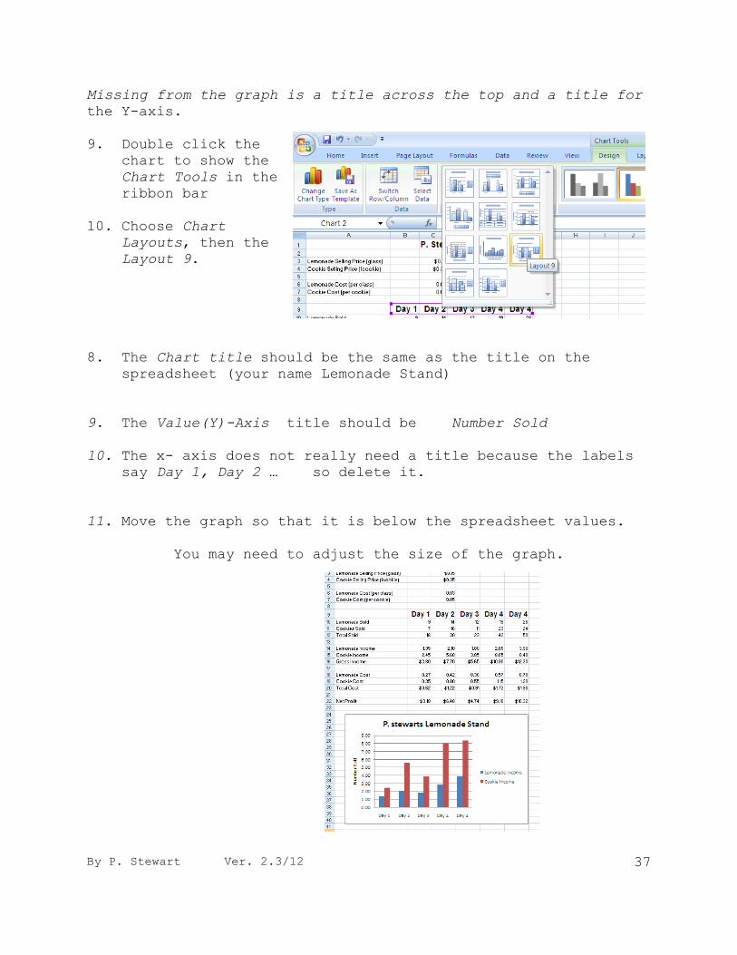
Missing from the graph is a title across the top and a title for
the Y-axis.
9. Double click the
chart to show the
Chart Tools in the
ribbon bar
10. Choose Chart Layouts, then the
Layout 9.
8. The Chart title should be the same as the title on the
spreadsheet (your name Lemonade Stand)
9. The Value(Y)-Axis title should be Number Sold
10. The x- axis does not really need a title because the labels say Day 1, Day 2 … so delete it.
11. Move the graph so that it is below the spreadsheet values.
You may need to adjust the size of the graph.
38 By P. Stewart Ver. 2.3/12
What IF calculations
One of the most powerful uses of the spreadsheet is the WHAT IF
projection.
Position the spreadsheet workspace so that you can see both the
graph and the lemonade sold row on the screen.
1. What IF the cookie sales double?
-Move to row 11 and double each of the cookie sales.
14, 32, 22, 46, 48
Notice the totals change as you enter each new value
and the graph changes too.
2. What If you increase the cookie price to 38 cents ?
-Move to cell C4 and change the cookie price.
The Total Income should change.
-View the graph, did the graph change? Why or why not?.
More changes
There are rumors of the government introducing an LST (Lemonade
Stand Tax) of 6% on Gross Income. What would happen to your net
sales if YOU decide to absorb this cost?
-Move to cell E6 and enter the label: LST %
-Move to cell F6 and enter .06
Format to Percent, 0 decimals
Note: That it now shows as a percent but you entered it as a
decimal number
By P. Stewart Ver. 2.3/12 39
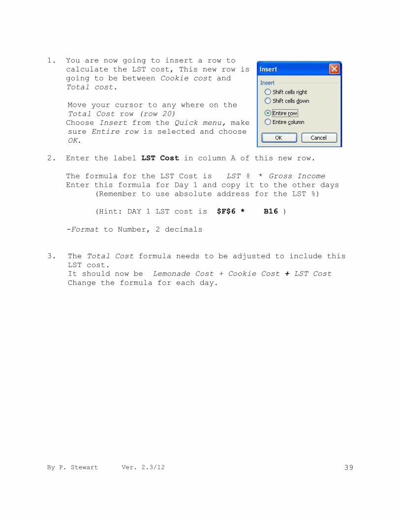
1. You are now going to insert a row to
calculate the LST cost, This new row is
going to be between Cookie cost and
Total cost.
Move your cursor to any where on the
Total Cost row (row 20)
Choose Insert from the Quick menu, make
sure Entire row is selected and choose
OK.
2. Enter the label LST Cost in column A of this new row.
The formula for the LST Cost is LST % * Gross Income
Enter this formula for Day 1 and copy it to the other days
(Remember to use absolute address for the LST %)
(Hint: DAY 1 LST cost is $F$6 * B16 )
-Format to Number, 2 decimals
3. The Total Cost formula needs to be adjusted to include this
LST cost.
It should now be Lemonade Cost + Cookie Cost + LST Cost
Change the formula for each day.
40 By P. Stewart Ver. 2.3/12
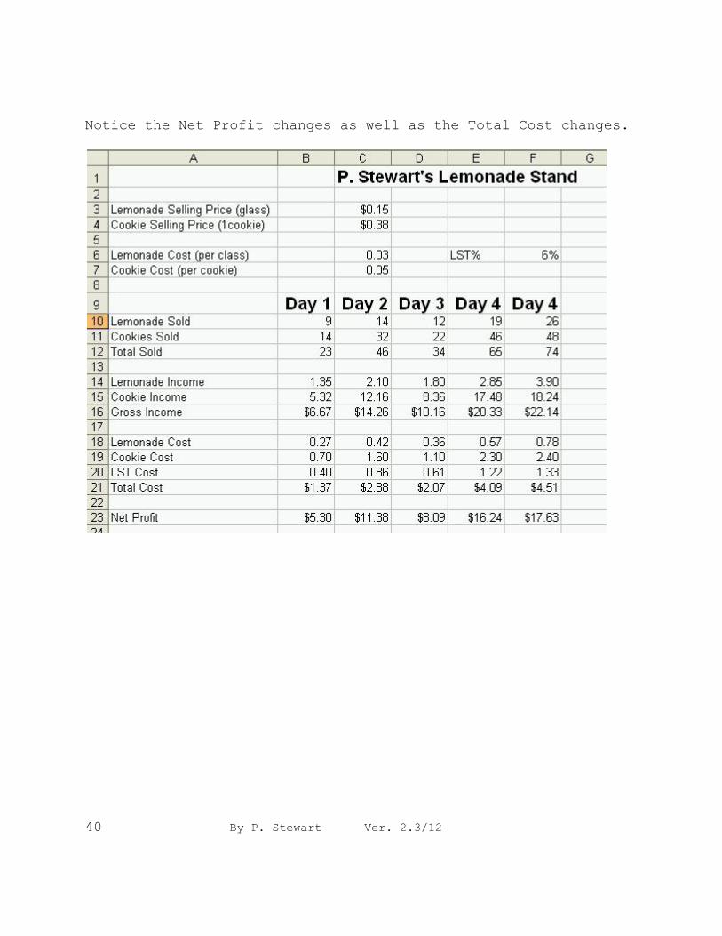
Notice the Net Profit changes as well as the Total Cost changes.
By P. Stewart Ver. 2.3/12 41
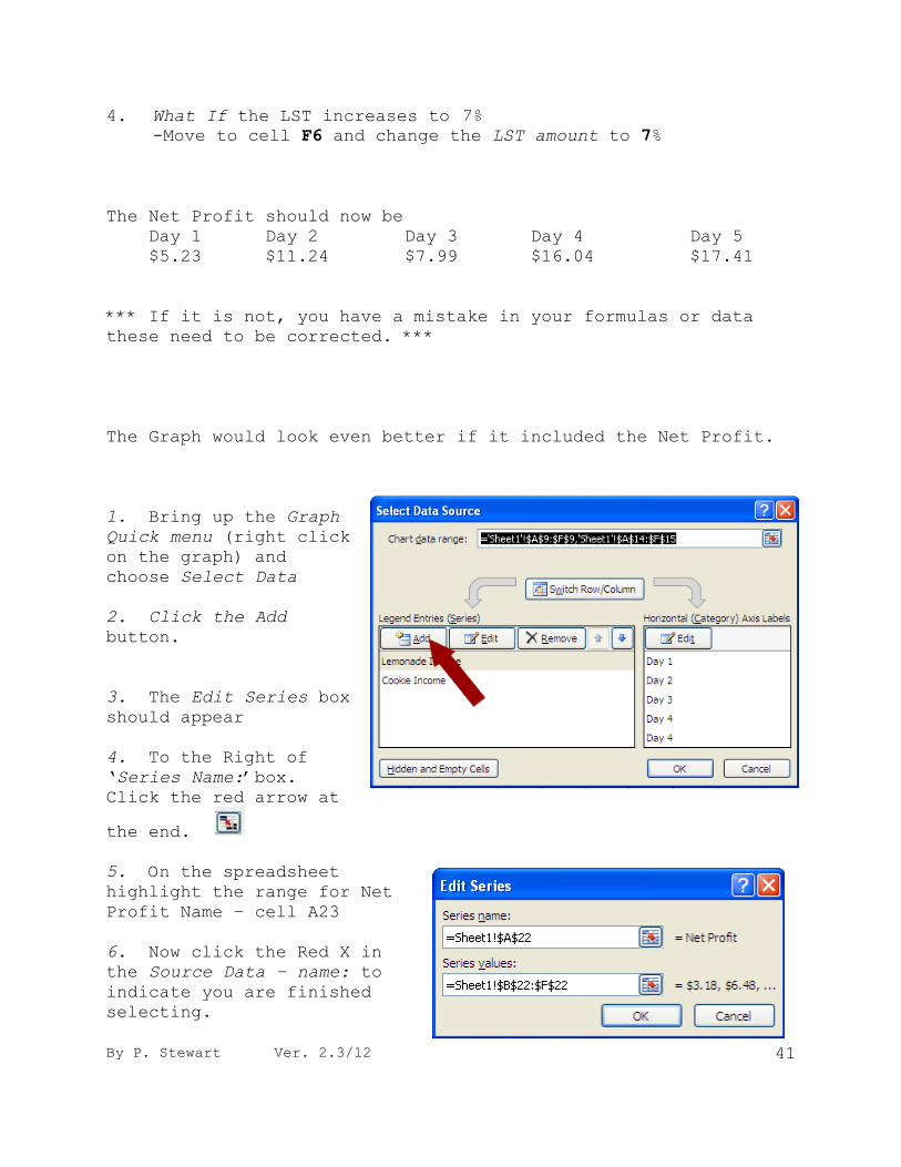
4. What If the LST increases to 7%
-Move to cell F6 and change the LST amount to 7%
The Net Profit should now be
Day 1 Day 2 Day 3 Day 4 Day 5
$5.23 $11.24 $7.99 $16.04 $17.41
*** If it is not, you have a mistake in your formulas or data
these need to be corrected. ***
The Graph would look even better if it included the Net Profit.
1. Bring up the Graph
Quick menu (right click
on the graph) and
choose Select Data
2. Click the Add
button.
3. The Edit Series box
should appear
4. To the Right of
„Series Name:‟box.
Click the red arrow at
the end.
5. On the spreadsheet
highlight the range for Net
Profit Name – cell A23
6. Now click the Red X in
the Source Data – name: to
indicate you are finished
selecting.
42 By P. Stewart Ver. 2.3/12
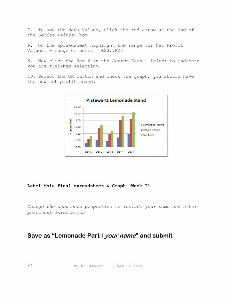
7. To add the data Values, click the red arrow at the end of
the Series Values: box
8. On the spreadsheet highlight the range for Net Profit
Values: – range of cells B23..F23
9. Now click the Red X in the Source Data – Value: to indicate
you are finished selecting.
10. Select the OK button and check the graph, you should have the new net profit added.
Label this final spreadsheet & Graph ‘Week I’
Change the documents properties to include your name and other
pertinent information
Save as “Lemonade Part I your name” and submit
By P. Stewart Ver. 2.3/12 43
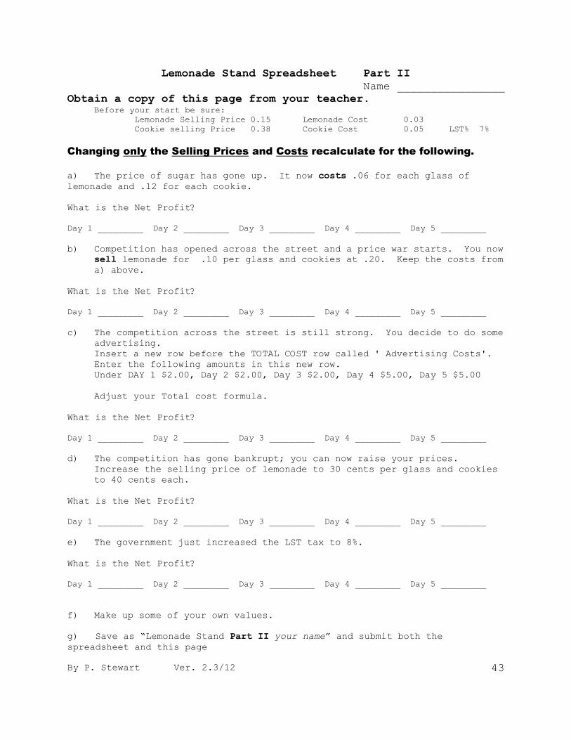
Lemonade Stand Spreadsheet Part II
Name ________________
Obtain a copy of this page from your teacher. Before your start be sure:
Lemonade Selling Price 0.15 Lemonade Cost 0.03
Cookie selling Price 0.38 Cookie Cost 0.05 LST% 7%
Changing only the Selling Prices and Costs recalculate for the following.
a) The price of sugar has gone up. It now costs .06 for each glass of
lemonade and .12 for each cookie.
What is the Net Profit?
Day 1 _________ Day 2 _________ Day 3 _________ Day 4 _________ Day 5 _________
b) Competition has opened across the street and a price war starts. You now
sell lemonade for .10 per glass and cookies at .20. Keep the costs from
a) above.
What is the Net Profit?
Day 1 _________ Day 2 _________ Day 3 _________ Day 4 _________ Day 5 _________
c) The competition across the street is still strong. You decide to do some
advertising.
Insert a new row before the TOTAL COST row called ' Advertising Costs'.
Enter the following amounts in this new row.
Under DAY 1 $2.00, Day 2 $2.00, Day 3 $2.00, Day 4 $5.00, Day 5 $5.00
Adjust your Total cost formula.
What is the Net Profit?
Day 1 _________ Day 2 _________ Day 3 _________ Day 4 _________ Day 5 _________
d) The competition has gone bankrupt; you can now raise your prices.
Increase the selling price of lemonade to 30 cents per glass and cookies
to 40 cents each.
What is the Net Profit?
Day 1 _________ Day 2 _________ Day 3 _________ Day 4 _________ Day 5 _________
e) The government just increased the LST tax to 8%.
What is the Net Profit?
Day 1 _________ Day 2 _________ Day 3 _________ Day 4 _________ Day 5 _________
f) Make up some of your own values.
g) Save as “Lemonade Stand Part II your name” and submit both the
spreadsheet and this page
44 By P. Stewart Ver. 2.3/12
Larry Lotospend Expense Report
Part I
Larry Lotospend is a businessman who does a lot of
traveling. He must keep an expense record. You are
to develop an expense report for Larry Lotsospend.
Larry's expense report should have one column for
each day of the week, Sunday through Saturday, and
an Items Totals column.
Note: You will have to adjust the column widths
EXPENSE REPORT
for Larry Lotospend May 7-13 (Created by your name)
ITEMS Sunday Monday Tuesday Wednesday Thursday Friday Saturday Total
Hotels
Meals
Air fare
Transportation
Parking
Entertainment
Misc.
Daily Total
By P. Stewart Ver. 2.3/12 45
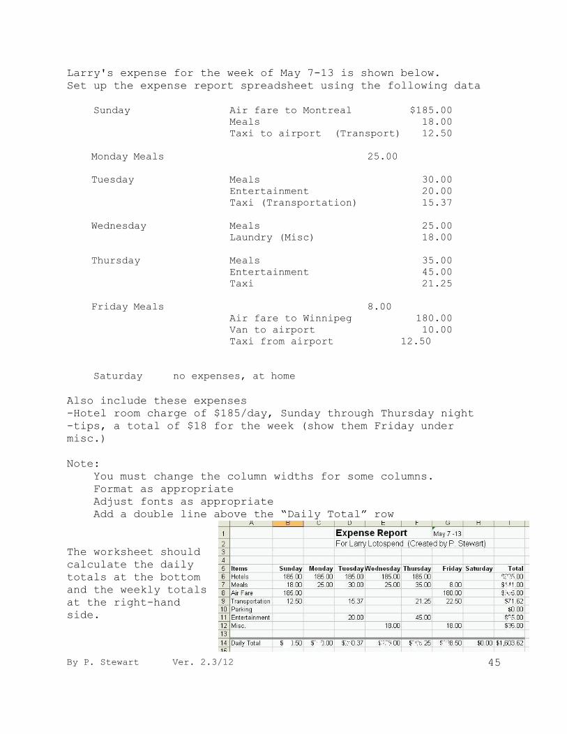
Larry's expense for the week of May 7-13 is shown below.
Set up the expense report spreadsheet using the following data
Sunday Air fare to Montreal $185.00
Meals 18.00
Taxi to airport (Transport) 12.50
Monday Meals 25.00
Tuesday Meals 30.00
Entertainment 20.00
Taxi (Transportation) 15.37
Wednesday Meals 25.00
Laundry (Misc) 18.00
Thursday Meals 35.00
Entertainment 45.00
Taxi 21.25
Friday Meals 8.00
Air fare to Winnipeg 180.00
Van to airport 10.00
Taxi from airport 12.50
Saturday no expenses, at home
Also include these expenses
-Hotel room charge of $185/day, Sunday through Thursday night
-tips, a total of $18 for the week (show them Friday under
misc.)
Note:
You must change the column widths for some columns.
Format as appropriate
Adjust fonts as appropriate
Add a double line above the “Daily Total” row
The worksheet should
calculate the daily
totals at the bottom
and the weekly totals
at the right-hand
side.
46 By P. Stewart Ver. 2.3/12
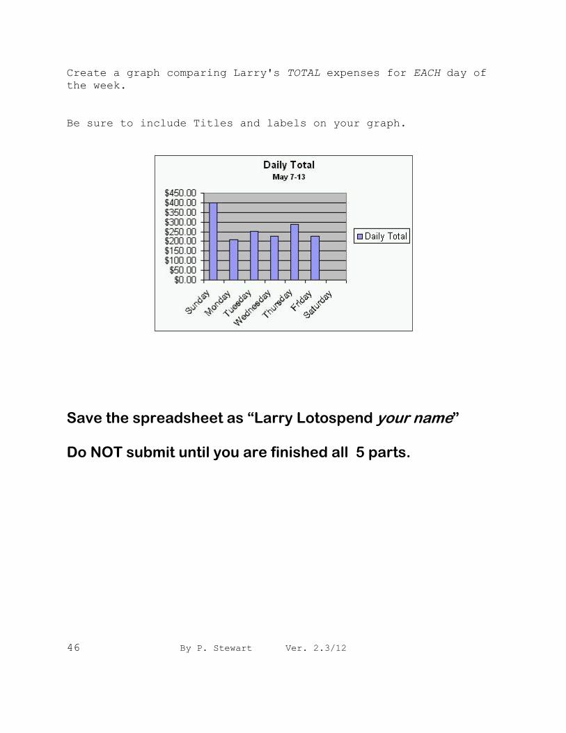
Create a graph comparing Larry's TOTAL expenses for EACH day of
the week.
Be sure to include Titles and labels on your graph.
Save the spreadsheet as “Larry Lotospend your name” Do NOT submit until you are finished all 5 parts.
By P. Stewart Ver. 2.3/12 47
Larry Lottospend Expense Report
Part II
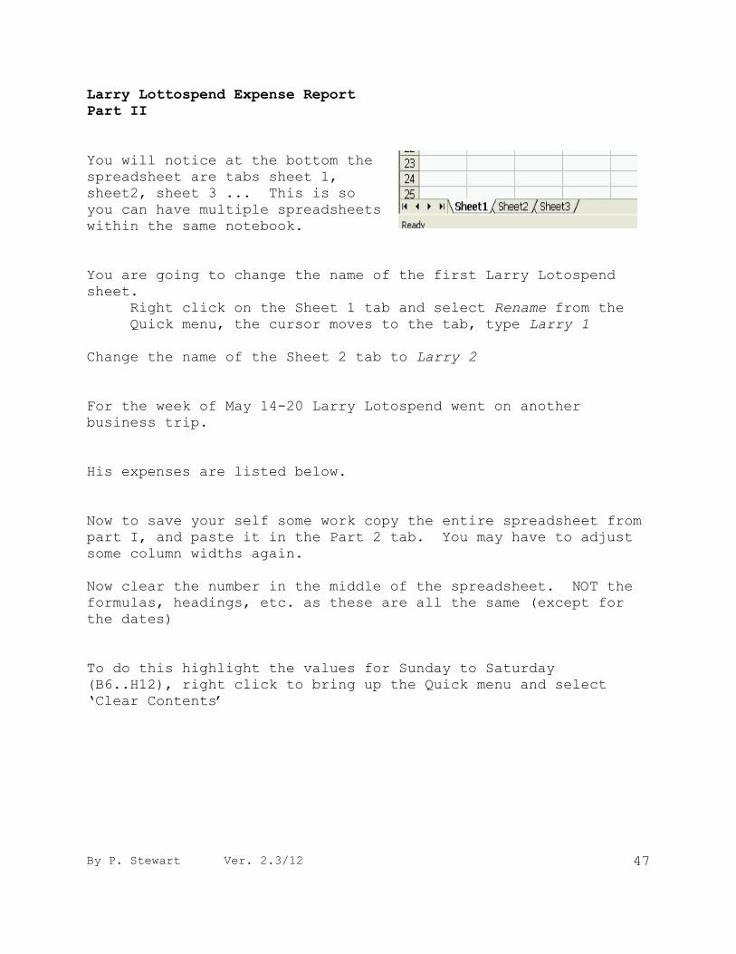
You will notice at the bottom the
spreadsheet are tabs sheet 1,
sheet2, sheet 3 ... This is so
you can have multiple spreadsheets
within the same notebook.
You are going to change the name of the first Larry Lotospend
sheet.
Right click on the Sheet 1 tab and select Rename from the
Quick menu, the cursor moves to the tab, type Larry 1
Change the name of the Sheet 2 tab to Larry 2
For the week of May 14-20 Larry Lotospend went on another
business trip.
His expenses are listed below.
Now to save your self some work copy the entire spreadsheet from
part I, and paste it in the Part 2 tab. You may have to adjust
some column widths again.
Now clear the number in the middle of the spreadsheet. NOT the
formulas, headings, etc. as these are all the same (except for
the dates)
To do this highlight the values for Sunday to Saturday
(B6..H12), right click to bring up the Quick menu and select
„Clear Contents‟
48 By P. Stewart Ver. 2.3/12
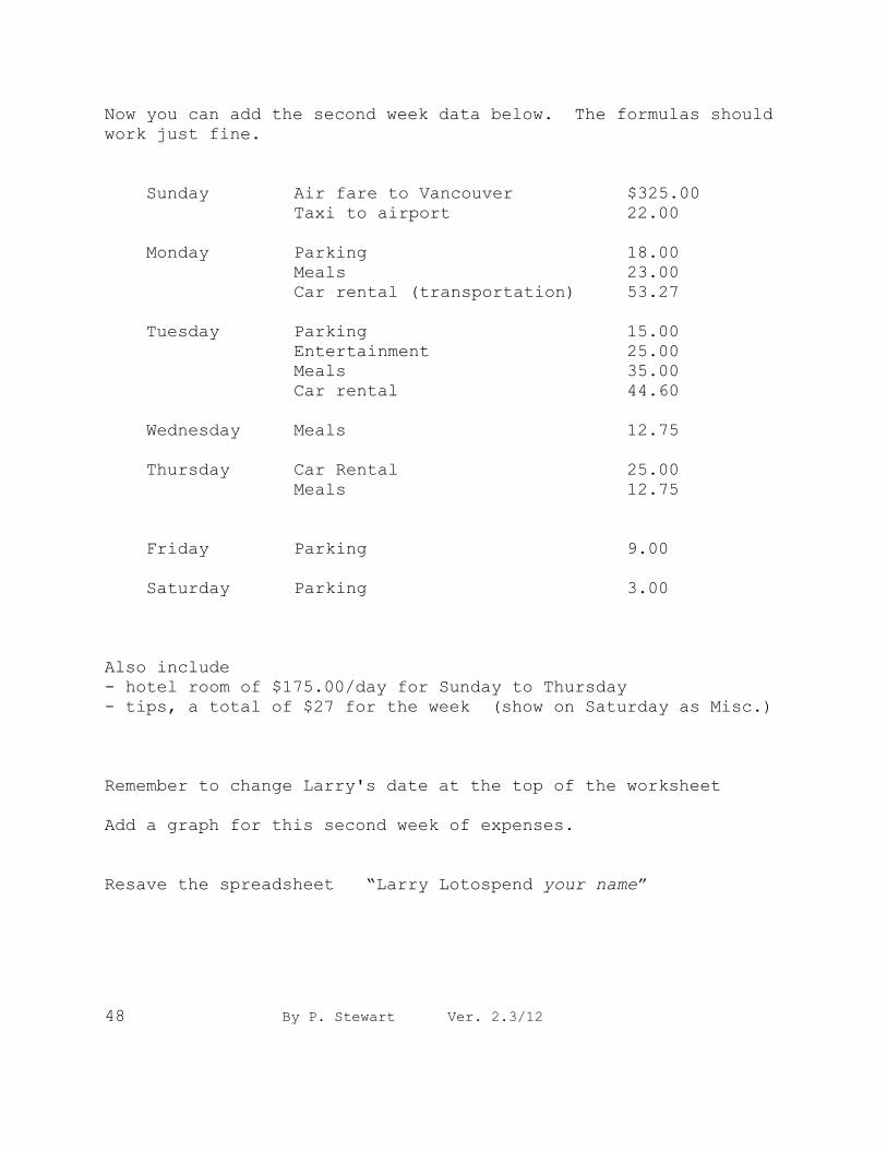
Now you can add the second week data below. The formulas should
work just fine.
Sunday Air fare to Vancouver $325.00
Taxi to airport 22.00
Monday Parking 18.00
Meals 23.00
Car rental (transportation) 53.27
Tuesday Parking 15.00
Entertainment 25.00
Meals 35.00
Car rental 44.60
Wednesday Meals 12.75
Thursday Car Rental 25.00
Meals 12.75
Friday Parking 9.00
Saturday Parking 3.00
Also include
- hotel room of $175.00/day for Sunday to Thursday
- tips, a total of $27 for the week (show on Saturday as Misc.)
Remember to change Larry's date at the top of the worksheet
Add a graph for this second week of expenses.
Resave the spreadsheet “Larry Lotospend your name”
By P. Stewart Ver. 2.3/12 49
Larry Lottospend Expense Report
Part III
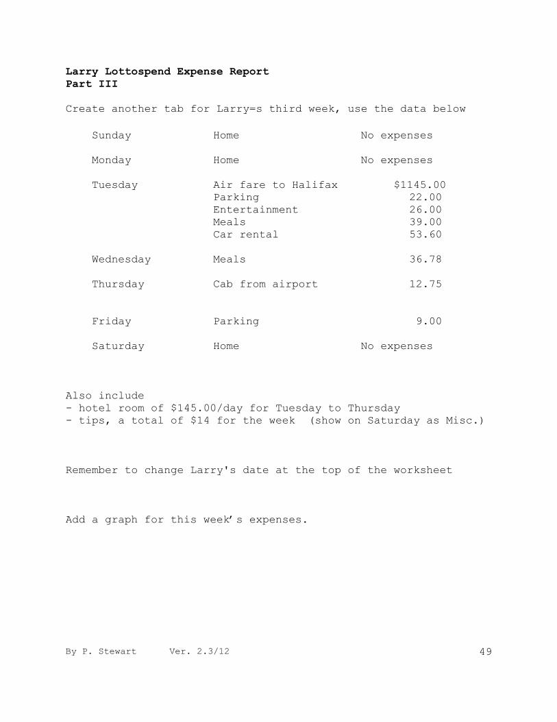
Create another tab for Larry=s third week, use the data below
Sunday Home No expenses
Monday Home No expenses
Tuesday Air fare to Halifax $1145.00
Parking 22.00
Entertainment 26.00
Meals 39.00
Car rental 53.60
Wednesday Meals 36.78
Thursday Cab from airport 12.75
Friday Parking 9.00
Saturday Home No expenses
Also include
- hotel room of $145.00/day for Tuesday to Thursday
- tips, a total of $14 for the week (show on Saturday as Misc.)
Remember to change Larry's date at the top of the worksheet
Add a graph for this week‟s expenses.
50 By P. Stewart Ver. 2.3/12
Larry Lottospend Expense Report
Part IV
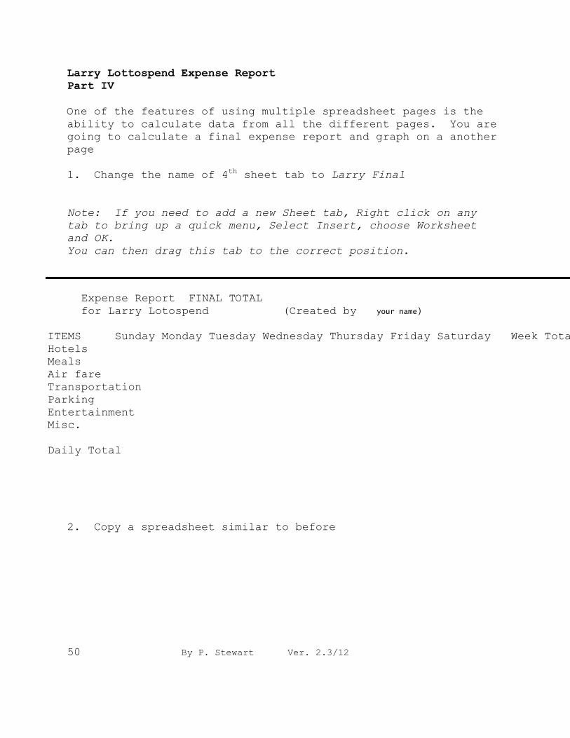
One of the features of using multiple spreadsheet pages is the
ability to calculate data from all the different pages. You are
going to calculate a final expense report and graph on a another
page
1. Change the name of 4th sheet tab to Larry Final
Note: If you need to add a new Sheet tab, Right click on any
tab to bring up a quick menu, Select Insert, choose Worksheet
and OK.
You can then drag this tab to the correct position.
2. Copy a spreadsheet similar to before
Expense Report FINAL TOTAL
for Larry Lotospend (Created by your name)
ITEMS Sunday Monday Tuesday Wednesday Thursday Friday Saturday Week Total
Hotels
Meals
Air fare
Transportation
Parking
Entertainment
Misc.
Daily Total
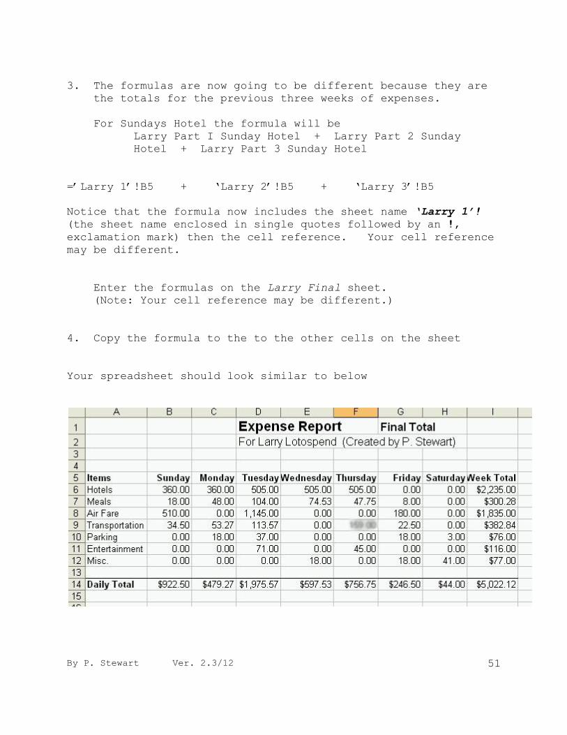
By P. Stewart Ver. 2.3/12 51
3. The formulas are now going to be different because they are
the totals for the previous three weeks of expenses.
For Sundays Hotel the formula will be
Larry Part I Sunday Hotel + Larry Part 2 Sunday
Hotel + Larry Part 3 Sunday Hotel
=‟Larry 1‟!B5 + „Larry 2‟!B5 + „Larry 3‟!B5
Notice that the formula now includes the sheet name ‘Larry 1’!
(the sheet name enclosed in single quotes followed by an !,
exclamation mark) then the cell reference. Your cell reference
may be different.
Enter the formulas on the Larry Final sheet.
(Note: Your cell reference may be different.)
4. Copy the formula to the to the other cells on the sheet
Your spreadsheet should look similar to below
52 By P. Stewart Ver. 2.3/12
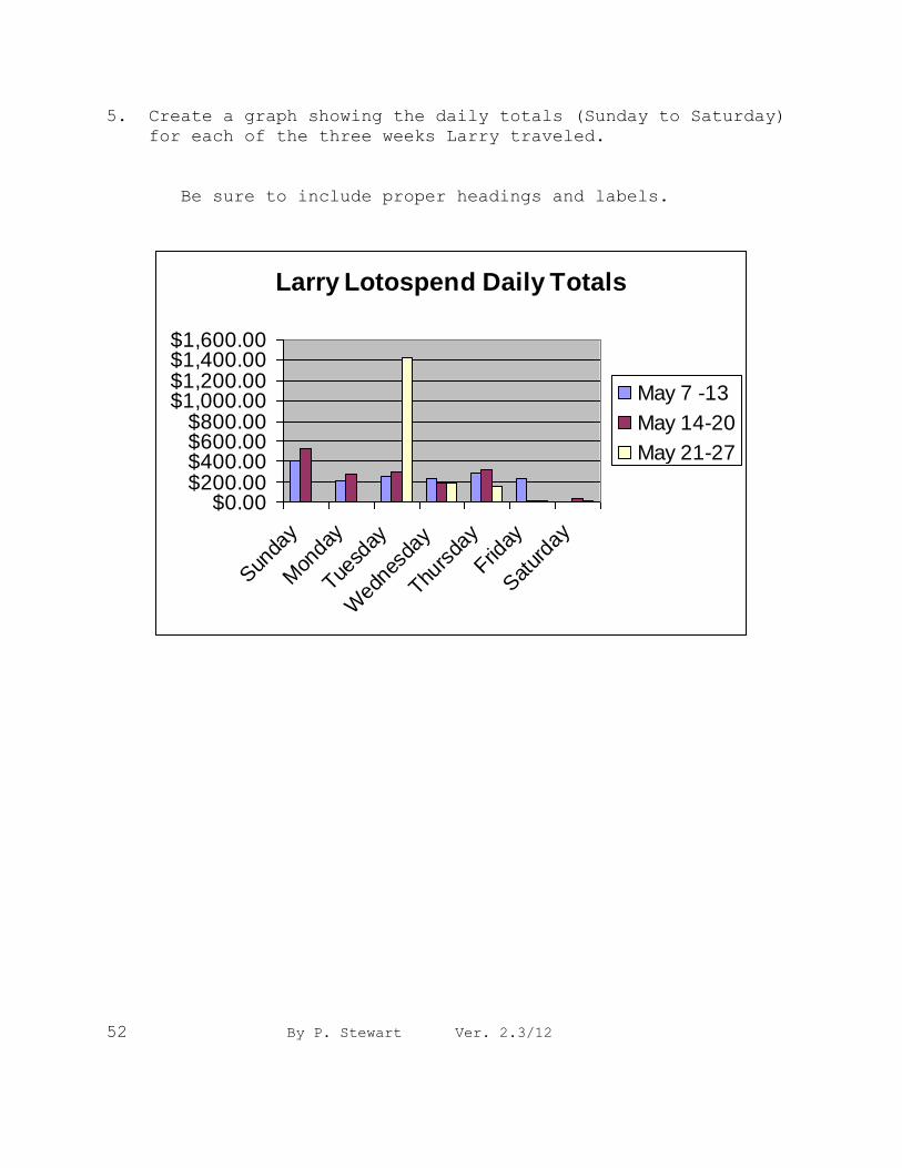
5. Create a graph showing the daily totals (Sunday to Saturday)
for each of the three weeks Larry traveled.
Be sure to include proper headings and labels.
Larry Lotospend Daily Totals
$0.00$200.00$400.00$600.00$800.00
$1,000.00$1,200.00$1,400.00$1,600.00
Sun
day
Mon
day
Tuesd
ay
Wed
nesd
ay
Thurs
day
Friday
Sat
urda
y
May 7 -13
May 14-20
May 21-27
By P. Stewart Ver. 2.3/12 53
Larry Lottospend Expense Report
Part V
There was a fourth week of travel for Larry. He flew to Las
Vegas for a conference from Monday to Friday.
-Create a fourth week of travel expenses, insert a new tab sheet
before the Larry Final sheet.
-You make up the expenses for this week
- Add a graph for this week‟s expenses.
-Modify the formulas on the Final sheet to include this new week
-Modify the graph to include this new week
-Label this spreadsheet and graph Part V.
-Change the documents properties to include your name and other
pertinent information
Save the spreadsheet as “Larry Lotospend your name” and submit
54 By P. Stewart Ver. 2.3/12
SPREADSHEET EXERCISE
Class Marks
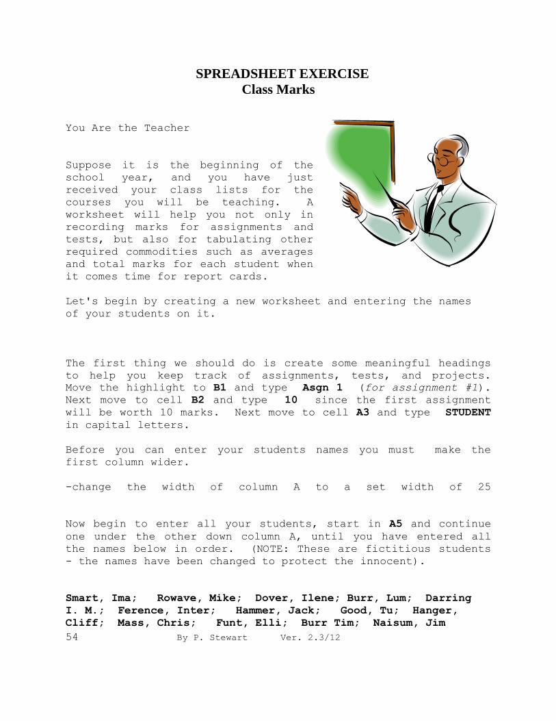
You Are the Teacher
Suppose it is the beginning of the
school year, and you have just
received your class lists for the
courses you will be teaching. A
worksheet will help you not only in
recording marks for assignments and
tests, but also for tabulating other
required commodities such as averages
and total marks for each student when
it comes time for report cards.
Let's begin by creating a new worksheet and entering the names
of your students on it.
The first thing we should do is create some meaningful headings
to help you keep track of assignments, tests, and projects.
Move the highlight to B1 and type Asgn 1 (for assignment #1).
Next move to cell B2 and type 10 since the first assignment
will be worth 10 marks. Next move to cell A3 and type STUDENT
in capital letters.
Before you can enter your students names you must make the
first column wider.
-change the width of column A to a set width of 25
Now begin to enter all your students, start in A5 and continue
one under the other down column A, until you have entered all
the names below in order. (NOTE: These are fictitious students
- the names have been changed to protect the innocent).
Smart, Ima; Rowave, Mike; Dover, Ilene; Burr, Lum; Darring
I. M.; Ference, Inter; Hammer, Jack; Good, Tu; Hanger,
Cliff; Mass, Chris; Funt, Elli; Burr Tim; Naisum, Jim
By P. Stewart Ver. 2.3/12 55
Well, it=s the second week of school now, it must be time for an
assignment - right? You decide that September 12 would be a
good day to collect an assignment. Move the highlight to B3 and
add the date as 09/12. Starting in cell B5 and moving down the
column, enter the following marks that are arranged to match the
students in order listed above:
8, 8.5, 7.5, 3.5, 4, 8.5, 9, 10, 10, 6, 10, 9,
9.5.
Format the above marks to Number, 1 decimal place.
Put your name to cell A1
Before going any further, now would be a good time to save your
work, use the filename "CLASS MARKS your name"
56 By P. Stewart Ver. 2.3/12
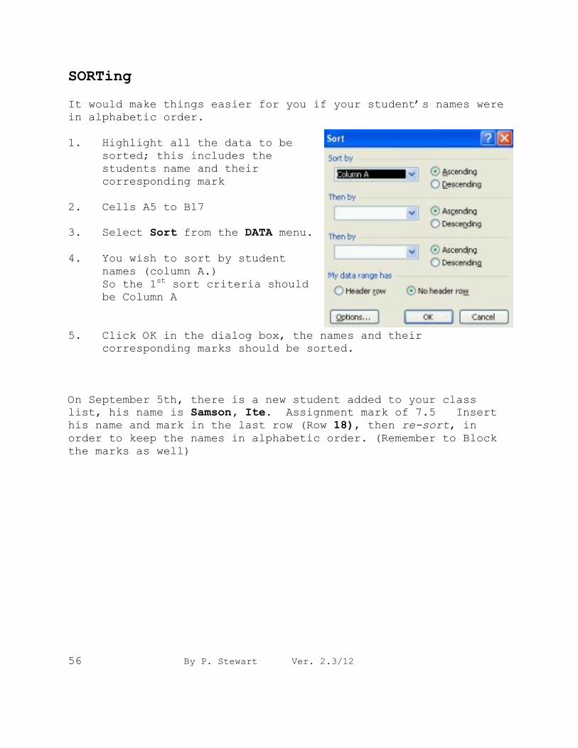
SORTing
It would make things easier for you if your student‟s names were
in alphabetic order.
1. Highlight all the data to be
sorted; this includes the
students name and their
corresponding mark
2. Cells A5 to B17
3. Select Sort from the DATA menu.
4. You wish to sort by student
names (column A.)
So the 1st sort criteria should
be Column A
5. Click OK in the dialog box, the names and their
corresponding marks should be sorted.
On September 5th, there is a new student added to your class
list, his name is Samson, Ite. Assignment mark of 7.5 Insert
his name and mark in the last row (Row 18), then re-sort, in
order to keep the names in alphabetic order. (Remember to Block
the marks as well)
By P. Stewart Ver. 2.3/12 57
More Changes
As a teacher, some information that would be valuable to have is
the average score for a test item, also the highest and lowest
mark. We can accomplish this be entering formulas into a cell.
1. Move the cursor down to cell B20
Here we want the average score, so enter the formula
=AVERAGE(B5.B19).
This formula instructs the worksheet program to start at
row 5 of the current column (B in this case), and add all
the numbers down to and including cell B19. Then the total
is divided by the number of cells used to arrive at the
average.
2. Now move down two cells and enter the formula for the lowest
(minimum) score. This time enter the formula =MIN(B5.B19)
3. Move down two more cells and enter the formula for the
highest (maximum) score, which is =MAX(B5.B19)
4. Change the format of the above three cells to Number, 1
decimal place.
5. Change the column width of column B to 7 characters.
6. Next you should include some labels to identify the
calculated numbers that will occupy these cells. In the
cell immediately to the left of where you placed the
average formula, enter the label Average Mark
7. Enter appropriate labels for the other two formulas entered
as well.
8. For appearance sake, you will want to have the labels you
just entered to be right justified instead of the default
that is left justified.
9. Do the same right align for the labels at the top of column B
58 By P. Stewart Ver. 2.3/12
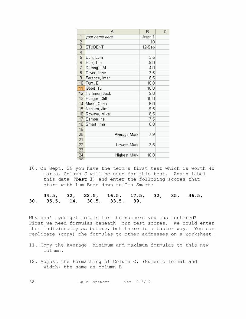
10. On Sept. 29 you have the term's first test which is worth 40
marks. Column C will be used for this test. Again label
this data (Test 1) and enter the following scores that
start with Lum Burr down to Ima Smart:
34.5, 32, 22.5, 16.5, 17.5, 32, 35, 36.5,
30, 35.5, 14, 30.5, 33.5, 39.
Why don't you get totals for the numbers you just entered?
First we need formulas beneath our test scores. We could enter
them individually as before, but there is a faster way. You can
replicate (copy) the formulas to other addresses on a worksheet.
11. Copy the Average, Minimum and maximum formulas to this new
column.
12. Adjust the Formatting of Column C, (Numeric format and
width) the same as column B
By P. Stewart Ver. 2.3/12 59
----------------------------------------------------------------
-
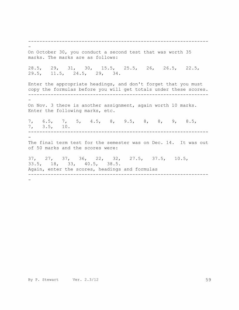
On October 30, you conduct a second test that was worth 35
marks. The marks are as follows:
28.5, 29, 31, 30, 15.5, 25.5, 26, 26.5, 22.5,
29.5, 11.5, 24.5, 29, 34.
Enter the appropriate headings, and don't forget that you must
copy the formulas before you will get totals under these scores.
----------------------------------------------------------------
-
On Nov. 3 there is another assignment, again worth 10 marks.
Enter the following marks, etc.
7, 6.5, 7, 5, 4.5, 8, 9.5, 8, 8, 9, 8.5,
7, 3.5, 10.
----------------------------------------------------------------
-
The final term test for the semester was on Dec. 14. It was out
of 50 marks and the scores were:
37, 27, 37, 36, 22, 32, 27.5, 37.5, 10.5,
33.5, 18, 33, 40.5, 38.5.
Again, enter the scores, headings and formulas
----------------------------------------------------------------
-
60 By P. Stewart Ver. 2.3/12
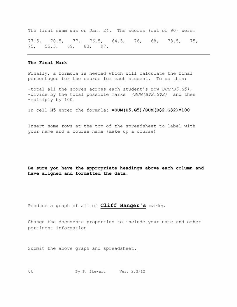
The final exam was on Jan. 24. The scores (out of 90) were:
77.5, 70.5, 77, 76.5, 64.5, 76, 68, 73.5, 75,
75, 55.5, 69, 83, 97.
The Final Mark
Finally, a formula is needed which will calculate the final
percentages for the course for each student. To do this:
-total all the scores across each student's row SUM(B5.G5),
-divide by the total possible marks /SUM(B$2.G$2) and then
-multiply by 100.
In cell H5 enter the formula: =SUM(B5.G5)/SUM(B$2.G$2)*100
Insert some rows at the top of the spreadsheet to label with
your name and a course name (make up a course)
Be sure you have the appropriate headings above each column and
have aligned and formatted the data.
Produce a graph of all of Cliff Hanger's marks.
Change the documents properties to include your name and other
pertinent information
Submit the above graph and spreadsheet.
By P. Stewart Ver. 2.3/12 61
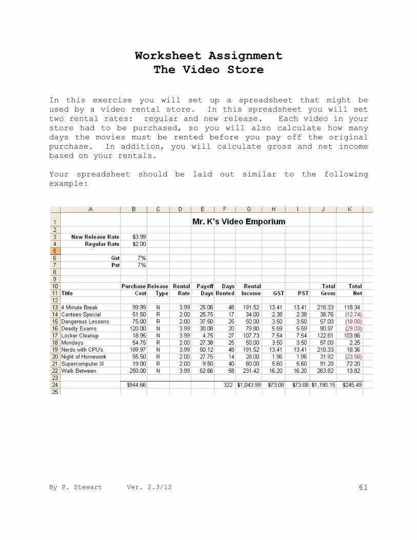
Worksheet Assignment
The Video Store
In this exercise you will set up a spreadsheet that might be
used by a video rental store. In this spreadsheet you will set
two rental rates: regular and new release. Each video in your
store had to be purchased, so you will also calculate how many
days the movies must be rented before you pay off the original
purchase. In addition, you will calculate gross and net income
based on your rentals.
Your spreadsheet should be laid out similar to the following
example:
62 By P. Stewart Ver. 2.3/12
DIRECTIONS:
- put the name of your store at the top of the spreadsheet
- Somewhere in the top few rows put the rates you will charge
for new releases and regular rent.
- Use the current rate for Provincial Sales Tax (PST) and Goods and Services Tax (GST). Be sure to enter all these
values as numbers, not text.
-Format the GST and PST as percent
-Format the New Release Rate and Regular Rate as currency, 2
decimals
- Before typing the labels for each column, change the width
of column A to 20 characters.
- Enter the labels for each column as they are in the
example.
-The label „Title‟ should be left justified, Right justified
the other labels
- Enter at least 12 titles of movies available in your store
(Make up your own names for the videos).
- Enter the price you paid for each video into the second
column.
-The third column is the Release Type.
In this column, enter the letter N if the movie is a New
release and R if it is a Regular release.
- In the next column, use a formula to call up the rent fee
for each title. Remember: the rental rates are in the top
rows. (By using a formula instead of just typing in the
rate, we can easily change our spreadsheet later).
The formula would be something like
=IF(C13=”N”, $B$3, $B$4)
Note: Your cell addresses may be a little different.
By P. Stewart Ver. 2.3/12 63
- In the Payoff Days column enter a formula to divide the
Purchase Cost by the Rental Rate to figure out the number of
days the movie must be rented before it is paid off.
- The fifth Column is the actual number of days the movies
were rented so far. Enter any values you wish for this
column.
- For the Rental Income column, enter a formula to multiply
the rental rate by the actual number of days rented to figure
out how many fees were collected.
- To calculate the taxes charge to your rent fees, multiply
the 'Rental Income' column by the cell that states the tax
rate (near the top of the spreadsheet). Be sure to use
ABSOLUTE ADDRESSES for the tax rate cell.
- Total Gross is the total money collected in your store.
Add the rental income and taxes to find this value.
- Total Net is the money that you have cleared. It is Gross
Income less purchase costs and taxes.
- One row below the spreadsheet, total all the columns except
Release Type, Rental Rate and Payoff days.
- Format these totals as Currency, 2 decimals
- Format the spreadsheet to make it look more professional.
E.g. Column Widths, fonts, bold, italics, borders, etc.
- Change the documents properties to include your name and other
pertinent information
64 By P. Stewart Ver. 2.3/12
To Do:
-Sort the movies in order by name.
-Change the rental rates until you find you are making
money.
-Produce a graph showing how the different movies compare
in the number of times each was rented.
-label the spreadsheet,save as “Movie Rental 1 your name”
and submit this spreadsheet.
-Change the rental Rate for new releases and regular
release.
- Also the government just changed the GST tax rate to
???? (make up your own).
-label the spreadsheet,save as “Movie Rental 2 your name”
and submit this spreadsheet.