micromorphic model - arxiv.org

A panorama of dispersion curves for the weighted isotropic relaxedmicromorphic model

Marco Valerio d’Agostino1and Gabriele Barbagallo2and Ionel-Dumitrel Ghiba3and Angela Madeo4 and Patrizio Neff 5

Dedicated to David J. Steigmann on the occasion of his 60th birthday

September 26, 2018

Abstract

We consider the weighted isotropic relaxed micromorphic model and provide an in depth investigation ofthe characteristic dispersion curves when the constitutive parameters of the model are varied. The weightedrelaxed micromorphic model generalizes the classical relaxed micromorphic model previously introduced by theauthors, since it features the Cartan-Lie decomposition of the tensors P,t and CurlP in their dev sym, skew andspheric part. It is shown that the split of the tensor P,t in the micro-inertia provide an independent control ofthe cut-offs of the optic banches. This is crucial for the future calibration of the relaxed micromorphic model onreal band-gap metamaterials.

Even if the physical interest of the introduction of the split of the tensor CurlP is less evident than inthe previous case, we discuss in detail which is its effect on the dispersion curves. Finally, we also provide acomplete parametric study involving all the constitutive parameters of the introduced model, so giving rise toan exhaustive panorama of dispersion curves for the relaxed micromorphic model.

Keywords: planar harmonic waves, relaxed micromorphic model, generalized continua, dynamic problem, micro-elasticity, size effects, wave propagation, band gaps.

AMS 2010 subject classification: 74A10 (stress), 74A30 (nonsimple materials), 74A35 (polar materials), 74A60(micromechanical theories), 74B05 (classical linear elasticity), 74M25 (micromechanics), 74Q15 (effective constitu-tive equations), 74J05 (Linear waves).

1Marco Valerio d’Agostino, corresponding author, [email protected], LGCIE, INSA-Lyon, Université de Lyon, 20avenue Albert Einstein, 69621, Villeurbanne cedex, France

2Gabriele Barbagallo, [email protected], LaMCoS-CNRS & LGCIE, INSA-Lyon, Universitité de Lyon, 20 avenueAlbert Einstein, 69621, Villeurbanne cedex, France

3Ionel-Dumitrel Ghiba, [email protected], Lehrstuhl für Nichtlineare Analysis und Modellierung, Fakultät für Mathematik,Universität Duisburg-Essen, Thea-Leymann Str. 9, 45127 Essen, Germany; Alexandru Ioan Cuza University of Iaşi, Department ofMathematics, Blvd. Carol I, no. 11, 700506 Iaşi, Romania; and Octav Mayer Institute of Mathematics of the Romanian Academy, IaşiBranch, 700505 Iaşi, Romania

4Angela Madeo, [email protected], LGCIE, INSA-Lyon, Université de Lyon, 20 avenue Albert Einstein, 69621, Villeurbannecedex, France

5Patrizio Neff, corresponding author, [email protected], Head of Chair for Nonlinear Analysis and Modelling, Fakultät fürMathematik, Universität Duisburg-Essen, Mathematik-Carrée, Thea-Leymann-Straße 9, 45127 Essen, Germany

1

arX

iv:1

610.

0329

6v1

[m

ath-

ph]

11

Oct

201

6

Contents1 Notation 4

2 Variational formulation of the relaxed model 52.1 Constitutive assumptions on the energy density and equations of motion in strong form . . . . . . . 62.2 Internal variable model . . . . . . . . . . . . . . . . . . . . . . . . . . . . . . . . . . . . . . . . . . . . 8

3 Limit passage to classical linear elasticity for vanishing micro-inertia 8

4 Plane wave propagation in isotropic relaxed micromorphic media 94.1 Analysis of dispersion curves . . . . . . . . . . . . . . . . . . . . . . . . . . . . . . . . . . . . . . . . 12

4.1.1 Cut-off frequencies . . . . . . . . . . . . . . . . . . . . . . . . . . . . . . . . . . . . . . . . . . 134.1.2 Oblique asymptotes . . . . . . . . . . . . . . . . . . . . . . . . . . . . . . . . . . . . . . . . . 134.1.3 Horizontal asymptotes . . . . . . . . . . . . . . . . . . . . . . . . . . . . . . . . . . . . . . . . 144.1.4 Tangents in 0 to the acoustic curves . . . . . . . . . . . . . . . . . . . . . . . . . . . . . . . . 17

5 Action of the material parameters on the behavior of the dispersion curves 185.1 Classical results . . . . . . . . . . . . . . . . . . . . . . . . . . . . . . . . . . . . . . . . . . . . . . . . 185.2 The classical relaxed micromorphic model and the internal variable model . . . . . . . . . . . . . . . 205.3 A panorama of dispersion curves for the weighted relaxed micromorphic model. . . . . . . . . . . . . 21

5.3.1 Case µc > 0, limα1→0

. . . . . . . . . . . . . . . . . . . . . . . . . . . . . . . . . . . . . . . . . . 21

5.3.2 Case µc > 0, limα2→0

. . . . . . . . . . . . . . . . . . . . . . . . . . . . . . . . . . . . . . . . . . 23

5.3.3 Case µc > 0, limα3→0

. . . . . . . . . . . . . . . . . . . . . . . . . . . . . . . . . . . . . . . . . . 24

5.3.4 Case µc > 0, limα2,α3→0

. . . . . . . . . . . . . . . . . . . . . . . . . . . . . . . . . . . . . . . . . 25

5.3.5 Vanishing Cosserat couple modulus µc = 0 and limα1→0 . . . . . . . . . . . . . . . . . . . . . 265.3.6 Vanishing Cosserat couple modulus µc = 0 and limα2→0 . . . . . . . . . . . . . . . . . . . . . 275.3.7 Vanishing Cosserat couple modulus µc = 0 and limα3→0 . . . . . . . . . . . . . . . . . . . . . 28

5.4 Variation of the micro-inertia weighting . . . . . . . . . . . . . . . . . . . . . . . . . . . . . . . . . . 295.4.1 Case η1 → 0 . . . . . . . . . . . . . . . . . . . . . . . . . . . . . . . . . . . . . . . . . . . . . . 295.4.2 Case η2 → 0 . . . . . . . . . . . . . . . . . . . . . . . . . . . . . . . . . . . . . . . . . . . . . . 305.4.3 Case η3 → 0 . . . . . . . . . . . . . . . . . . . . . . . . . . . . . . . . . . . . . . . . . . . . . . 305.4.4 Cases η1,η2, η3 → 0: the fundamental role of the micro-inertia for enriched continuum mechanics 315.4.5 Case η1 → +∞ . . . . . . . . . . . . . . . . . . . . . . . . . . . . . . . . . . . . . . . . . . . . 325.4.6 Case η2 → +∞ . . . . . . . . . . . . . . . . . . . . . . . . . . . . . . . . . . . . . . . . . . . . 335.4.7 Case η3 → +∞ . . . . . . . . . . . . . . . . . . . . . . . . . . . . . . . . . . . . . . . . . . . . 345.4.8 Cases η1,η2, η3 → +∞: a rigidified Cauchy material . . . . . . . . . . . . . . . . . . . . . . . 35

5.5 Other interesting cases . . . . . . . . . . . . . . . . . . . . . . . . . . . . . . . . . . . . . . . . . . . . 365.5.1 Case µe → +∞ and Lc decreasing . . . . . . . . . . . . . . . . . . . . . . . . . . . . . . . . . 365.5.2 Case µe, µmicro, µc → +∞ . . . . . . . . . . . . . . . . . . . . . . . . . . . . . . . . . . . . . . 375.5.3 Case µmicro → +∞ “Cosserat limit” . . . . . . . . . . . . . . . . . . . . . . . . . . . . . . . . . 375.5.4 Case µmicro, µc → +∞ and η → 0 “indeterminate couple stress theory” . . . . . . . . . . . . . 37

6 Acknowledgments 39

7 Appendix 407.1 Variation of the kinetic energy . . . . . . . . . . . . . . . . . . . . . . . . . . . . . . . . . . . . . . . 407.2 Variation of the part B of the potential energy . . . . . . . . . . . . . . . . . . . . . . . . . . . . . . 417.3 Derivation of PDEs in the new variables . . . . . . . . . . . . . . . . . . . . . . . . . . . . . . . . . . 417.4 Determination of slopes of the acoustic branches . . . . . . . . . . . . . . . . . . . . . . . . . . . . . 477.5 Derivation of strong equations for the Cosserat model and indeterminate couple stress model . . . . 47

2

IntroductionThe micromorphic framework is increasingly used as an algorithmic device to regularize gradient-elasticity or gradi-ent plasticity models (see e.g. [12, 13]). In these cases, the problem of understanding the genuine physical meaningwhich can be associated to micromorphic models does not arise, since the micromorphic framework is simply usedas a tool for the regularization of higher order models. With a completely different perspective, in a series ofworks [24, 25, 20, 26], we started looking for real situations in which micromorphic models can be used to properlyconvey important physical informations to the modeling of the actual mechanical behavior of some microstructuredmaterials. More particularly, we focused our attention on the newly introduced relaxed micromorphic model6 (see[1, 15, 30, 31, 32, 36, 35]) to investigate the unorthodox dynamical properties of band-gap metamaterials, i.e. mi-crostructured materials which are able to inhibit wave propagation in precise frequency ranges. Similarly to theclassical micromorphic models originally introduced by Mindlin and Eringen [28, 10], the relaxed micromorphicmodel features an enriched kinematics to account e.g. for microscopic motions in the interior of the consideredmacroscopic continuum. Additionally to the classical macroscopic displacement vector field u(x, t), the micromor-phic models typically introduce supplementary, microstructure-related, degrees of freedom by means of a secondorder tensor field P (x, t) which is known as micro-distortion tensor. The relaxed micromorphic model differs frommore classical micromorphic ones in the sense that the higher order space derivatives of the field P are consti-tutively introduced in the strain energy density not through the whole gradient of P , but only through its Curl.The fact of using the Curl of the micro-distortion tensor is rather common when dealing with dislocation basedgradient plasticity (see e.g. [6, 2, 3, 4, 5, 8, 9, 7, 11, 17, 33, 38, 40, 42]), but this is indeed not the case whenconsidering pure elasticity in which the standard formulations commonly introduce the whole gradient ∇P of themicro-distortion tensor P . As a matter of fact, the use of micromorphic models which only consider the Curl ofthe micro-distortion in a purely linear-elastic framework can shed light on the modeling of non-local metamaterialswhich exhibit band-gap behaviors [24, 25, 20, 26, 23, 22, 21].

In the present work, we provide a generalization of the isotropic relaxed micromorphic model used in [24, 25, 20,26] based on the Cartan-Lie decomposition of the micro-distortion tensor P and of its Curl. Such decompositionallows us to introduce, in the isotropic setting, three parameters for the micro-inertia and three internal lengthassociated to the space derivatives of P appearing through CurlP . If the physical meaning of the three micro-inertia parameters may be rather intuitively related to a distinction of the weights attributed to the distortional,rotational and volumetric expansion vibration modes at the level of the unit cell, a clear interpretation of theintroduction of three different characteristic lengths is less immediate. In the view of applications, we will be ableto show in the short term whether it is worth introducing three different micro-inertia parameters for real band-gapmetamaterials. The phenomenological interest of the actual distinction of the non-localities associated to threedifferent internal lengths will be also investigated in further works.

In this paper, we discuss the effect that the introduced split of the micro-inertia and of the internal lengths hason the dispersion curves of the considered relaxed micromorphic model. We present and discuss in detail the specificeffects that the micro-inertia parameters and the characteristic lengths have on the characteristic of the dispersioncurves, in general, and of the band-gaps, in particular. The split on the micro-inertia is found to be fundamentalfor the description of real metamaterials, since it gives the possibility of controlling separately the cut-offs of theoptic curves in the dispersion diagram.

We obtain the previously introduced results [25] with a unique micro-inertia parameter and internal length as asuitable limiting case of the more general model presented here. We then focus our attention on another particularlimiting case that is the one with vanishing internal lengths. Such particular case of the relaxed micromorphicmodel in which no derivatives of the micro-distortion tensor appear can be called as an “internal variable model”(in the Cosserat framework this approach has been named “reduced Cosserat model”, see [18, 16]) and may be ofinterest for the description of some band gap metamaterials for which the so-called hypothesis of separation of scalesis verified (see e.g. [41, 39]).

For all the proposed cases, we show the direct effect of the variation of any single parameter on the dispersioncurves and on the band gap characteristics. This paper is now organized as follows:

• in chapter 1 we introduce the notations used in the paper,

• in chapter 2 we present the weighted relaxed micromorphic model in the unbounded domain R3 in a variationalform and we derive the PDEs governing the system,

6We use the term relaxed in its proper english meaning and not in the sense of finding the lower semi-continuous hull. Indeed, therelaxed micromorphic continuum is always lower semi-continuous, but, contrary to the classical micromorphic model, the assumptionon the constitutive coefficients are much weakened (relaxed). Notably, constraining the micro-distortion P = ∇u does not lead to asecond-gradient model but leads back to classical linear elasticity without characteristic length scale.

3

• in chapter 3 we show how it is possible to recover the classical linear elasticity model from the relaxedmicromorphic model,

• in chapter 4 we introduce the plane wave ansatz on the unknown kinematical fields in order to show how it ispossible to reduce the system of governing PDEs to an algebraic problem, finding also the dispersion curves.

• in chapter 5 we perform a parametric study on the influence of the material parameters on the behavior ofthe dispersion curves.

1 NotationThroughout this paper the Einstein convention of sum over repeated indexes is used if not differently specified. Wedenote by R3×3 the set of real 3×3 second order tensors and by R3×3×3 the set of real 3×3×3 third order tensors.The standard Euclidean scalar product on R3×3 is given by 〈X,Y 〉 R3×3 = tr(X ·Y T ) and, thus, the Frobenius tensornorm is ‖X‖2 = 〈X,X〉 R3×3 . Moreover, the identity tensor on R3×3 will be denoted by 1, so that tr(X) = 〈X,1〉.We adopt the usual abbreviations of Lie-algebra theory, i.e.:

• Sym (3) := X ∈ R3×3 |XT = X denotes the vector-space of all symmetric 3× 3 matrices

• so (3) := X ∈ R3×3 |XT = −X is the Lie-algebra of skew symmetric tensors

• sl(3) := X ∈ R3×3 |tr(X) = 0 is the Lie-algebra of traceless tensors

• R3×3 ' gl(3) = sl(3) ∩ Sym (3) ⊕ so (3)⊕ R·1 is the orthogonal Cartan-decomposition of the Lie-algebra

In other words, for all X ∈ R3×3, we consider the decomposition

X = dev symX + skewX +1

3tr(X)1 (1)

where:

• symX = 12 (XT +X) ∈ Sym (3) is the symmetric part of X,

• skewX = 12 (X −XT ) ∈ so (3) is the skew-symmetric part of X,

• devX = X − 13 tr(X)1 ∈ sl(3) is the deviatoric part of X.

Throughout this paper we denote:

• the sixth order tensors L : R3×3×3 → R3×3×3, by a hat,

• the fourth order tensors C : R3×3 → R3×3, by an overline,

• without superscripts, the classical fourth order tensors acting only on symmetric matricesC : Sym (3)→ Sym (3) or skew-symmetric ones Cc : so (3)→ so (3) ,

• the second order tensors Cc : R3 → R3 appearing as elastic stiffness, by a tilde.

We denote by CX the linear application of a 4th order tensor to a 2nd order tensor and also for the linear applicationof a 6th order tensor L to a 3rd order tensor. In symbols, we have:(

CX)ij

= CijhkXhk ,(LA

)ijh

= LijhpqrApqr . (2)

The operation of simple contraction between tensors of suitable order is denoted by a central dot as, for example:(C · v

)i

= Cijvj ,(C ·X

)ij

= CihXhj . (3)

Typical conventions for differential operations are implied such as a comma followed by a subscript to denote thepartial derivative with respect to the corresponding Cartesian coordinate, i.e. (·),j = ∂(·)

∂xj.

4

The curl of a vector field v is defined as7(curl v)i = εijkvk,j ,

where εijk is the Levi-Civita third order permutation tensor. Let X be a two order tensor field and X1, X2, X3

three vector fields such that

X =

XT1

XT2

XT3

.

The Curl of X is defined as follows:

CurlX =

(curlX1)T

(curlX2)T

(curlX3)T

,

that in indices is(CurlX)ij = εjmnXin,m.

For the iterated Curl we find

(Curl Curl P )ij = εjmn (CurlP )in,m = εjmn (εnabPib,a),m = εjmnεnabPib,am

= − εnmjεnabPib,am = (δmaδjb − δmbδja)Pib,am = Pim,jm − Pij,mm.

The divergence div v of a vector field v is defined as div v = vi,i and the divergence DivX of a matrix X as

DivX =

divX1

divX2

divX3

=

(X1)i,i(X2)i,i(X3)i,i

.

Given two differentiable vector fields u, v : Ω ⊆ R3 → R3, we have that

div (u× v) = 〈curlu, v〉 − 〈u, curl v〉 , (4)

since

(εijkujvk),i = εijkuj,ivk + εijkujvk,i = εkijuj,ivk − ujεjikvk,i= 〈curlu, v〉 − 〈u, curl v〉 .

2 Variational formulation of the relaxed modelThe kinematical fields of the problem are the displacement u and the micro-distortion tensor field P :

u : Ω× I → R3, (x, t) 7→ u (x, t) , P : Ω× I → R3×3, (x, t) 7→ P (x, t) ,

where Ω is an open bounded domain in R3 with a piecewise smooth boundary ∂Ω and closure Ω, and I = [0, T ] ⊆ Ris the time interval. The mechanical model is formulated in the variational context. This means that we consideran action functional on an appropriate function-space. Setting Ω0 = Ω × 0, the space of configurations of theproblem is

Q :=

(u, P ) ∈ C 1(Ω× I,R3

)× C 1

(Ω× I,R3×3

): (u, P ) verifies conditions (B1) and (B2)

where

• (B1) are the boundary conditions u (x, t) = ϕ (x, t) and Pi (x, t)×n = ψi (x, t), i = 1, 2, 3, (x, t) ∈ ∂Ω×[0, T ],where n is the unit outward normal vector on ∂Ω × [0, T ], Pi, i = 1, 2, 3 are the rows of P and ϕ,ψi areprescribed functions,

• (B2) are the initial conditions u|Ω0= u0, u,t|Ω0

= u0, P |Ω0= P0, P,t|Ω0

= P 0 in Ω0, where u0 (x) , u0 (x) ,P0 (x) , P 0 (x) are prescribed functions.

7Given a third order tensors A and a second order tensor B, the double contraction A : B is defined as (A : B)i = AijkBkj .

5

The action functional A : Q → R, is the sum of the internal and external action functionals A intL ,A ext : Q → R

defined as follows

A intL [(u, P )] :=

∫I

∫Ω

L (u,t, P,t,∇u, P,CurlP ) dv dt, (5)

A ext [(u, P )] :=

∫I

∫Ω

(⟨fext, u

⟩+⟨Mext, P

⟩)dv dt,

where L is the Lagrangian density of the system and fext,Mext are the body force and double body force. In thiswork we will consider fext = 0,Mext = 0. In order to find the stationary points of the action functional, we haveto calculate its first variation:

δA = δA intL = δ

∫I

∫Ω

L (u,t, P,t,∇u, P,CurlP ) dv dt.

Well-posedness of this variational problem (existence, uniqueness and stability of solution) has been proved in[15, 36, 35].

2.1 Constitutive assumptions on the energy density and equations of motion instrong form

For the Lagrangian energy density we assume the standard split in kinetic minus potential energy:

L (u,t, P,t,∇u, P,CurlP ) = J (u,t, P,t)−W (∇u, P,CurlP ) ,

In general anisotropic linear elastic micromorphic media, as clearly stated in [1, 36], we have that the kinetic energydensity and the potential have the following expression

J (u,t, P,t) =1

2〈ρ u,t, u,t〉+

1

2

⟨J P,t, P,t

⟩W (∇u, P,CurlP ) =

1

2〈Ce sym (∇u− P ) , sym (∇u− P )〉R3×3︸︷︷︸

anisotropic elastic - energy

+1

2〈Cmicro symP, symP 〉R3×3︸︷︷︸

micro - self - energy

+1

2〈Cc skew (∇u− P ) , skew (∇u− P )〉R3×3︸︷︷︸

invariant local anisotropic rotational elastic coupling

+µL2c

2

⟨Laniso CurlP,CurlP

⟩R3×3︸︷︷︸

curvature

,

where

ρ : Ω→ R+ is the macro-inertia density,J : R3×3 → R3×3 is the 4thorder micro-inertia density tensor,Ce,Cmicro : Sym (3)→ Sym (3) are the 4thorder elasticity tensors with 21 independent components,Cc : so (3)→ so (3) is a dimensionless 4th order tensor with 6 independent components,Laniso : R3×3 → R3×3 is a dimensionless 4th order tensor with almost 45 independent components,

and Lc is the characteristic length of the relaxed micromorphic model. We demand that the bilinear forms inducedby J,Ce,Cmicro,Laniso are positive definite,

∃ c+, c+e , c+micro, c+l > 0 : ∀S ∈ Sym(3)

⟨J S, S

⟩R3×3 ≥ c+‖S‖2R3×3 ,

〈Ce S, S〉 R3×3 ≥ c+e ‖S‖2R3×3 ,

〈Cmicro S, S〉 R3×3 ≥ c+micro‖S‖2R3×3 ,⟨Laniso S, S

⟩R3×3 ≥ c+l ‖S‖2R3×3 ,

(6)

and, in sharp contrast to the Mindlin-Eringen format, that the bilinear form induced by Cc is only positive semi-definite, i.e.8

∀A ∈ so (3) :⟨Cc A,A

⟩R3×3 ≥ 0. (7)

8It is in virtue of such weakening of the theoretical framework needed to prove its well posedness that the word “relaxed” was chosento distinguish the relaxed micromorphic model from Mindlin’s one (see [1, 15, 30, 31, 32, 36, 35]).

6

In this work we introduce the hypothesis according to which the micromorphic medium is homogeneous andisotropic. This leads to the following particular expression for the kinetic and strain energy densities:

J (u,t, P,t) =1

2ρ ‖u,t‖2 +

1

2

(η 1 ‖dev symP,t‖2 + η 2 ‖skewP,t‖2 +

1

3η 3 (trP,t)

2

),

W (∇u, P,CurlP ) = µe ‖sym (∇u− P )‖2 +λe2

(tr (∇u− P ))2

+ µmicro ‖symP‖2 +λmicro

2(trP )

2+µc ‖skew (∇u− P )‖2︸︷︷︸

A

+ µeL2c

2

(α1 ‖dev symCurlP‖2 + α2 ‖skewCurlP‖2 +

1

3α3 (tr CurlP )

2

)︸︷︷︸

B

, (8)

where ρ is the macroscopic mass density, Lc is the internal length accounting for non-local effects, µc is the Cosseratcouple modulus, µe, λe, µmicro, λmicro are the other elastic parameters featured by the isotropic relaxed micromorphicmodel (see [36]), η1, η2, η3 are the inertia weights and α1, α2, α3 are dimensionless parameters. It can be seen thatthe two tensor fields P,t and CurlP have been decomposed according to the Cartan-Lie decomposition. Since thepart A of the potential energy is the same as in [25], in order to compute the first variation of the action functionalit is sufficient to evaluate only the first variation of the kinetic energy and the second part B of the potential energy.

We explicitly remark that the chosen expression for the micro-inertia in terms of η1, η2 and η3 is more generalthan the one introduced in [25]. The same holds for the non-local term in which the three constants α1, α2 and α3

appear. A crucial point for further experimentally oriented works will be the split of the kinetic energy that weintroduce here. Indeed, the fact of introducing three micro-inertia parameters instead of one allows extra freedomfor the fitting of the dispersion curves on real band-gap metamaterials.

The particular case of the relaxed micromorphic model presented in [25] can be obtained by simply settingη1 = η2 = η3 = 10−2 Kg/m, and α1 = α2 = α3 = 1. The weights α1, α2 and α3 allow to account for a refinedsplitting of the non-localities present in the considered relaxed micromorphic model. This possibility provides acertain freedom for future developments, but it is too general to provide new physical understanding of band-gapmetamaterials currently studied. In fact, the most common band-gap metamaterials are conceived letting non-localeffects being very small based on some sort of “separation of scales” hypothesis (see e.g. [39, 41]). This means it issensible that, for such metamaterials, non-local effects may be described by means of a unique characteristic length(case α1 = α2 = α3 = 1). Nevertheless, the weighted higher-order terms presented here may allow for more detaileddescriptions of non-localities in new metamaterials in which strong contrasts of the mechanical properties at themicro-level occur.

The question is quite different for the isotropic weighted expression of the micro-inertia which introduces the 3parameters η1, η2 and η3. It is indeed sensible that, for some metamaterials, the vibrations associated to distortion,rotation and volumetric expansion of the unit cells at the micro-level do not occur with the same facility. In otherwords, the three different modes might be more or less privileged depending on the considered metamaterial.

The real interest of the presented micro-inertia splitting must be tested by fitting the proposed relaxed micro-morphic model on real experiments on existing band-gap metamaterials. We leave this task to a forthcoming paper,limiting ourselves here to discuss numerical results which may be of interest for conceiving pertinent experimentalcampaigns.

We have shown elsewhere [15, 31, 32, 35], that the static and dynamic problem in a bounded domain is well-posed(existence and uniqueness) under the general assumptions on the constitutive coefficients:

3λe + 2µe > 0, µe > 0, µmicro > 0, 3λmicro + 2µmicro > 0, J is positive definite,

ρ > 0, µc ≥ 0, Lc > 0 and α1, α2 > 0, α3 ≥ 0.(9)

Currently, it is not known whether assuming only

(α1, α2 > 0, α3 ≥ 0) or (α1 > 0, α2, α3 ≥ 0) (10)

is sufficient for well-posedness of the initial boundary value problem. In our parametric study of the whole-spaceharmonic wave propagation problem (11), we will re-encounter the limit case (10) showing no deficiency.

It is straightforward to derive (with the stronger regularity for the kinematical fields (u, P ) ∈ C 2(Ω× I,R3

)×

C 2(Ω× I,R3×3

)) the Euler-Lagrange equations corresponding to the Lagrangian associated with the strain energy

and kinetic energies (8) which, after projection on the orthogonal subspaces in (1), read9:9The new calculations concerning the variation of the term B in (8) are presented in Appendix 1

7

ρ u,tt = Div [2µe sym (∇u− P ) + λe tr (∇u− P )1 + 2µc skew (∇u− P )] ,

η 1 dev symP,tt = 2µe dev sym (∇u− P )− 2µmicro dev symP

− µe L2c dev sym

(α1 Curl dev symCurlP + α2 Curl skewCurlP +

α3

3Curl (tr (CurlP )1)

),

η 2 skewP,tt = 2µc skew (∇u− P ) (11)

− µe L2c skew

(α1 Curl dev symCurlP + α2 Curl skewCurlP +

α3


),

1

3η 3 tr (P,tt) =

(2

3µe + λe

)tr (∇u− P )−

(2

3µmicro + λmicro

)tr (P )

− µe L2c

1

3tr(α1 Curl dev symCurlP + α2 Curl skewCurlP +

α3


).

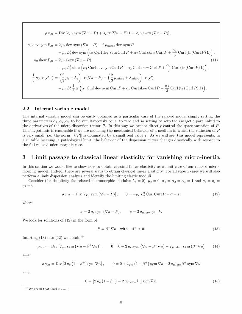
2.2 Internal variable modelThe internal variable model can be easily obtained as a particular case of the relaxed model simply setting thethree parameters α1, α2, α3 to be simultaneously equal to zero and so setting to zero the energetic part linked tothe derivatives of the micro-distortion tensor P . In this way we cannot directly control the space variation of P .This hypothesis is reasonable if we are modeling the mechanical behavior of a medium in which the variation of Pis very small, i.e. the norm ‖∇P‖ is dominated by a small real value ε. As we will see, this model represents, ina suitable meaning, a pathological limit: the behavior of the dispersion curves changes drastically with respect tothe full relaxed micromorphic case.

3 Limit passage to classical linear elasticity for vanishing micro-inertiaIn this section we would like to show how to obtain classical linear elasticity as a limit case of our relaxed micro-morphic model. Indeed, there are several ways to obtain classical linear elasticity. For all shown cases we will alsoperform a limit dispersion analysis and identify the limiting elastic moduli.

Consider (for simplicity the relaxed micromorphic modulus λe = 0), µc = 0, α1 = α2 = α3 = 1 and η1 = η2 =η3 = 0.

ρ u,tt = Div [2µe sym (∇u− P )] , 0 = −µe L2c CurlCurlP + σ − s, (12)

where

σ = 2µe sym (∇u− P ) , s = 2µmicro symP.

We look for solutions of (12) in the form of

P = β+∇u with β+ > 0. (13)

Inserting (13) into (12) we obtain10

ρ u,tt = Div[2µe sym

(∇u− β+∇u

)], 0 = 0 + 2µe sym

(∇u− β+∇u

)− 2µmicro sym

(β+∇u

)(14)

⇐⇒

ρ u,tt = Div[2µe

(1− β+

)sym∇u

], 0 = 0 + 2µe

(1− β+

)sym∇u− 2µmicro β

+ sym∇u

⇐⇒

0 =[2µe

(1− β+

)− 2µmicro β

+]sym∇u. (15)

10We recall that Curl∇u = 0.

8

Since sym∇u 6= 0 by assumption, equation (15) is verified if and only if

2µe(1− β+

)− 2µmicro β

+ = 0,

this means

µe(1− β+

)= µmicro β

+ ⇐⇒ µeµmicro

=β+

1− β+⇐⇒ β+ =

µeµe + µmicro

. (16)

Assuming generically that µe < µmicro, we find the following inequalities

β+

1− β+=

µeµmicro

< 1 ⇔ β+ < 1− β+ ⇔ 2β+ < 1 ⇔ β+ <1

2.

Inserting the last expression of β+ in (16) we find

ρ u,tt = Div[2µe(1− β+

)︸︷︷︸=

µmicro

µe +µmicro

sym∇u]

and therefore

ρ u,tt = Div[2

µe µmicro

µe + µmicrosym∇u

]= Div [2µmacro sym∇u] , (17)

where we have setµmacro :=

µe µmicro

µe + µmicro(harmonic mean),

according to formula (50) in [1]. This analysis can be repeated with λe 6= 0 such that 2µe + 3λe > 0. In this casewe obtain as limit model

ρ u,tt = Div [2µmacro sym∇u+ λmacro tr (∇u)1] (18)

withµmacro :=

µe µmicro

µe + µmicro, λmacro =

1

3

(2µe + 3λe) (2µmicro + 3λmicro)

2 (µe + µmicro) + 3 (λe + λmicro)− 2

3

µe µmicro

µe + µmicro

being consistent with

κmacro =2µmacro + 3λmacro

3

from [1]. Thus the relaxed micromorphic model with µc = 0 and η ≡ 0 provides a classical macroscopic, first gradientsolution with µmacro, λmacro as elastic moduli, provided that the micro-inertia is identically zero (or η → 0).

4 Plane wave propagation in isotropic relaxed micromorphic mediaIn this section we introduce the plane wave ansatz on the unknown kinematical fields. This hypothesis allows tostudy the main characteristics of wave propagation of relaxed micromorphic media in the simplest possible way.The problem of wave propagation still remains 3D (all the components of the introduced unknown fields are nonvanishing), while the space dependence is only on one scalar direction x1 which is also the direction of propagationof the plane wave. Under this assumption, the bulk equations (11) take a simplified form because all the partialderivatives in x2, x3-direction are zero.

Moreover, thanks to an opportune change of variables, we can completely uncouple the system of PDE in (11)as done in [25]. In order to do this, we project also the micro-distortion tensor P on the component spaces of theCartan-Lie decomposition of R3×3. We set for the deviatoric - symmetric part

dev symP =1

2

(P + PT

)− 1

3tr (P )1 =

PD1 P(12) P(13)

P(12) PD2 P(23)

P(13) P(23) PD3

, (19)

where we have defined

PDα = Pαα −1

3trP, and P(αβ) = P(βα) =

1

2(Pαβ + Pβα) if α 6= β. (20)

9

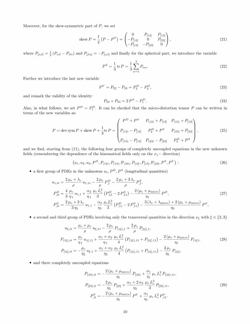
Moreover, for the skew-symmetric part of P , we set

skewP =1

2

(P − PT

)=

0 P[12] P[13]

−P[12] 0 P[23]

−P[13] −P[23] 0

, (21)

where P[αβ] = 12 (Pαβ − Pβα) and P[βα] = −P[αβ] and finally for the spherical part, we introduce the variable

PS =1

3trP =

1

3

3∑α=1

Pαα. (22)

Further we introduce the last new variable

PV = P22 − P33 = PD2 − PD3 , (23)

and remark the validity of the identityP22 + P33 = 2PS − PD1 . (24)

Also, in what follows, we set PD = PD1 . It can be checked that the micro-distortion tensor P can be written interms of the new variables as:

P = dev symP + skewP +1

3trP =

PD + PS P(12) + P[12] P(13) + P[13]

P(12) − P[12] PD2 + PS P(23) + P[23]

P(13) − P[13] P(23) − P[23] PD3 + PS

, (25)

and we find, starting from (11), the following four groups of completely uncoupled equations in the new unknownfields (remembering the dependence of the kinematical fields only on the x1− direction)(

u1, u2, u3, PD, P(12), P(13),P(23), P[12], P[13],P[23], P

S , PV)

: (26)

• a first group of PDEs in the unknowns u1, PD, PS (longitudinal quantities)

u1,tt =2µe + λe

ρu1,11 −

2µeρ

PD,1 −2µe + 3λe

ρPS,1,

PD,tt =4

3

µeη 1

u1,1 +α2

η 1

µe L2c

3

(PD,11 − 2PS,11

)− 2 (µe + µmicro)

η1PD, (27)

PS,tt =2µe + 3λe

3 η3u1,1 −

α2

η3

µeL2c

3

(PD,11 − 2PS,11

)− 3 (λe + λmicro) + 2 (µe + µmicro)

η3PS ,

• a second and third group of PDEs involving only the transversal quantities in the direction xξ with ξ ∈ 2, 3

uξ,tt =µe + µc

ρuξ,11 −

2µeρ

P(1ξ),1 +2µcρ

P[1ξ],1,

P(1ξ),tt =µeη 1

u(ξ,1) +α1 + α2

η 1

µe L2c

4

(P(1ξ),11 + P[1ξ],11

)− 2 (µe + µmicro)

η1P(1ξ), (28)

P[1ξ],tt = −µcη2uξ,1 +

α1 + α2

η2

µe L2c

4

(P(1ξ),11 + P[1ξ],11

)− 2µc

η2P[1ξ],

• and three completely uncoupled equations

P(23),tt = −2 (µe + µmicro)

η1P(23) +

α1

η1µe L

2c P(23),11,

P[23],tt = −2µcη2

P[23] +α1 + 2α3

η2

µe L2c

3P[23],11, (29)

PV,tt = −2 (µe + µmicro)

η1PV +

α1

η1µe L

2c P

V,11.

10

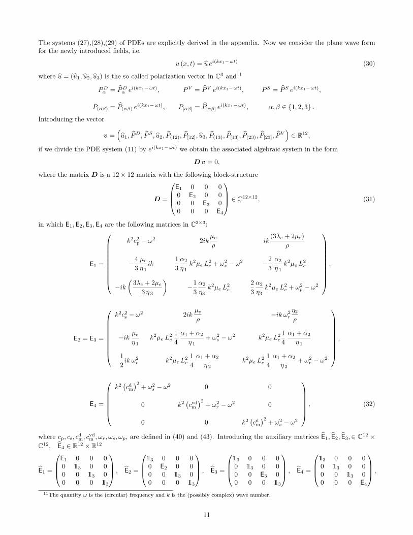
The systems (27),(28),(29) of PDEs are explicitly derived in the appendix. Now we consider the plane wave formfor the newly introduced fields, i.e.

u (x, t) = u ei(kx1−ωt) (30)

where u = (u1, u2, u3) is the so called polarization vector in C3 and11

PDα = PDα ei(kx1−ωt), PV = PV ei(kx1−ωt), PS = PS ei(kx1−ωt),

P(αβ) = P(αβ) ei(kx1−ωt), P[αβ] = P[αβ] e

i(kx1−ωt), α, β ∈ 1, 2, 3 .

Introducing the vector

v =(u1, P

D, PS , u2, P(12), P[12], u3, P(13), P[13], P(23), P[23], PV)∈ R12,

if we divide the PDE system (11) by ei(kx1−ωt) we obtain the associated algebraic system in the form

Dv = 0,

where the matrix D is a 12× 12 matrix with the following block-structure

D =

E1 0 0 00 E2 0 00 0 E3 00 0 0 E4

∈ C12×12, (31)

in which E1,E2,E3,E4 are the following matrices in C3×3:

E1 =

k2c2p − ω2 2ikµeρ

ik(3λe + 2µe)

ρ

−4

3

µeη 1ik

1

3

α2

η 1k2µe L

2c + ω2

s − ω2 −2

3

α2

η 1k2µe L

2c

−ik(

3λe + 2µe3 η 3

)−1

3

α2

η3k2µe L

2c

2

3

α2

η3k2µe L

2c + ω2

p − ω2

,

E2 = E3 =

k2c2s − ω2 2ikµeρ

−ik ω2r

η2

ρ

−ik µeη 1

k2µe L2c

1

4

α1 + α2

η 1+ ω2

s − ω2 k2µe L2c

1

4

α1 + α2

η 1

1

2ik ω2

r k2µe L2c

1

4

α1 + α2

η 2k2µe L

2c

1

4

α1 + α2

η 2+ ω2

r − ω2

,

E4 =

k2(cdm)2

+ ω2s − ω2 0 0

0 k2(cvdm)2

+ ω2r − ω2 0

0 0 k2(cdm)2

+ ω2s − ω2

, (32)

where cp, cs, cdm, cvdm , ωr, ωs, ωp, are defined in (40) and (43). Introducing the auxiliary matrices E1, E2, E3,∈ C12 ×

C12, E4 ∈ R12 × R12

E1 =

E1 0 0 00 13 0 00 0 13 00 0 0 13

, E2 =

13 0 0 00 E2 0 00 0 13 00 0 0 13

, E3 =

13 0 0 00 13 0 00 0 E3 00 0 0 13

, E4 =

13 0 0 00 13 0 00 0 13 00 0 0 E4

,

11The quantity ω is the (circular) frequency and k is the (possibly complex) wave number.

11

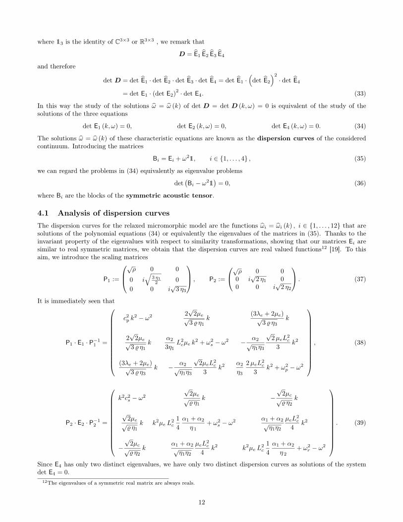
where 13 is the identity of C3×3 or R3×3 , we remark that

D = E1 E2 E3 E4

and therefore

det D = det E1 · det E2 · det E3 · det E4 = det E1 ·(

det E2

)2

· det E4

= det E1 · (det E2)2 · det E4. (33)

In this way the study of the solutions ω = ω (k) of det D = det D (k, ω) = 0 is equivalent of the study of thesolutions of the three equations

det E1 (k, ω) = 0, det E2 (k, ω) = 0, det E4 (k, ω) = 0. (34)

The solutions ω = ω (k) of these characteristic equations are known as the dispersion curves of the consideredcontinuum. Introducing the matrices

Bi = Ei + ω21, i ∈ 1, . . . , 4 , (35)

we can regard the problems in (34) equivalently as eigenvalue problems

det(Bi − ω21

)= 0, (36)

where Bi are the blocks of the symmetric acoustic tensor.

4.1 Analysis of dispersion curvesThe dispersion curves for the relaxed micromorphic model are the functions ωi = ωi (k) , i ∈ 1, . . . , 12 that aresolutions of the polynomial equations (34) or equivalently the eigenvalues of the matrices in (35). Thanks to theinvariant property of the eigenvalues with respect to similarity transformations, showing that our matrices Ei aresimilar to real symmetric matrices, we obtain that the dispersion curves are real valued functions12 [19]. To thisaim, we introduce the scaling matrices

P1 :=

√ρ 0 0

0 i√

3 η12 0

0 0 i√

3 η3

, P2 :=

√ρ 0 00 i

√2 η1 0

0 0 i√

2 η2

. (37)

It is immediately seen that

P1 · E1 · P−11 =

c2p k2 − ω2 2

√2µe√

3 % η1k

(3λe + 2µe)√3 % η3

k

2√

2µe√3 % η1

kα2

3η1L2cµe k

2 + ω2s − ω2 − α2√

η1η3

√2µeL

2c

3k2

(3λe + 2µe)√3 % η3

k − α2√η1η3

√2µeL

2c

3k2 α2

η3

2µeL2c

3k2 + ω2

p − ω2

, (38)

P2 · E2 · P−12 =

k2c2s − ω2

√2µe√% η1

k −√

2µc√% η2

k

√2µe√% η1

k k2µe L2c

1

4

α1 + α2

η 1+ ω2

s − ω2 α1 + α2√η1η2

µeL2c

4k2

−√

2µc√% η2

kα1 + α2√η1η2

µeL2c

4k2 k2µe L

2c

1

4

α1 + α2

η 2+ ω2

r − ω2

. (39)

Since E4 has only two distinct eigenvalues, we have only two distinct dispersion curves as solutions of the systemdet E4 = 0.

12The eigenvalues of a symmetric real matrix are always reals.

12

4.1.1 Cut-off frequencies

The cut-off frequencies are the solutions of the equation detD (k, ω) = 0 when k = 0 and give us the values of thedispersion curves ωi (k) at k = 0. We find only three different non trivial solutions for the equation detD (0, ω) = 0 :

ωs (µe, µmicro, η1) =

√2 (µe + µmicro)

η1, ωr (µc, η2) =

√2µcη2

,

(40)

ωp (λe, λmicro, µe, µmicro, η3) =

√3 (λe + λmicro) + 2 (µe + µmicro)

η3,

with multiplicity of 5,3,1, respectively. The null solution has multiplicity 3. This means that if

• µc > 0 we have 3 acoustic curves, and 9 optic curves,

• µc = 0 we have 6 acoustic curves, and 6 optic curves.

The first novel result with respect to [25] is that the presence of three micro-inertia terms η1, η2, η3 makes the threecut-off frequencies completely independent. This means that having fixed the parameters (λe, λmicro, µe, µmicro, µc)we can obtain all positive values for the cut-offs by simply changing the values of the three inertia parametersη1, η2, η3. Whether the fact of having η1 6= η2 6= η3 may be interesting for applications on real band-gap metama-terials must be checked on real experiments. It will be the objective of a forthcoming paper to show that this isindeed the case.

4.1.2 Oblique asymptotes

In this sub-section we want to give a tool to determine the oblique asymptotes to the unbounded dispersion curvesω (k), solutions of the equation det D (k, ω) = 0. First of all, it is useful to notice that the matrix D can be writtenas:

D (k, ω) = A2 k2 + B2 ω

2 + A1 k + C0,

where A2,B2,A1 and C0 are suitable 12× 12 constant real matrices with B2 invertible. Thus we have that

det D (k, ω) = det(A2 k

2 + B2 ω2 + A1 k + C0

)= det B2 · det

(B−1

2 A2 k2 + ω21+ B−1

2 A1 k + B−12 C0

)= k24 detB2 · det

(B−1

2 A2 +ω2

k21+

1

kB−1

2 A1 +1

k2B−1

2 C0

).

Thus the equation det D (k, ω) = 0 is equivalent to

p (k, ω) = det

(B−1

2 A2 +ω2

k21+

1

kB−1

2 A1 +1

k2B−1

2 C0

)= 0. (41)

Proposition 1. Let us assume that the equation det D (k, ω) = 0 admits a non-empty set of solutions ∆ =

ωi (k)n∈Ni=1 . Let us consider the subset ∆∞ = ωjs≤nj=1 constituted by the solutions verifying the following conditions:

1. ωj is a monotonically increasing function of k for j = 1, . . . , s,

2. limk→∞ωj(k)k 6= 0 for j = 1, . . . , s, (which implies that ωj is unbounded and so without horizontal asymptote),

and we assume that ∆∞ 6= Ø. If we consider a reduced problem

q (k, ω) = det

(B−1

2 A2 +(ωk

)2

1

)= 0, (42)

then this problem (42) admits solutions ωj (k)sj=1 such that limk→∞ (ωj − ωj) = 0 for every j = 1, . . . , s.

Proof. This is a simple application of the property of the continuous dependence of the roots of a polynomial onits coefficients. We can remark that under condition 2 of the proposition, if we think the coefficients of p (k, ω) asfunctions of k (because we are looking for solutions of the type k 7→ (k, ω (k))), then due to the continuity of thedeterminant, they converge to the coefficients of q (k, ω) and so do its roots.

13

Remark 2. Proposition 1 does not work for the bounded dispersion curves because in this case also the term ω(k)k

converges to zero when k → ∞ because bounded curves violate the conditions 2 of proposition 1. It is for thisreason that we will give another argument to look for the horizontal asymptotes.

In our case the roots ωj (k) of the reduced polynomial (42) can be computed more easily and are found to bestraight lines with slopes:

cdm =

√α1 µe L2

c

η1, cvd

m =

√(α1 + 2α3) µe L2

c

3 η2, cdr

m =1

2

√(η1 + η2)

η1 η2(α1 + α2) µe L2

c ,

(43)

cs =

√µe + µc

ρ, cp =

√2µe + λe

ρ, crm =

√(2 η1 + η3)

3 η1 η3α2 µe L2

c .

4.1.3 Horizontal asymptotes

In this subsection we want to investigate the behavior at infinity of the dispersion curves that are bounded i.e.that have horizontal asymptote. Thus, let ω (k) be a bounded solution of the equation detD (k, ω) = 0. Under theassumption that this function is monotonically increasing in k, setting

ω∗ := supR+

ω (k) <∞,

it is straightforward to show that ω (k) admit a horizontal asymptote whose value is ω∗. Thanks to the particularexpression of the function detD (k, ω) we can find a necessary (and computable) condition on ω∗ both in the generalrelaxed micromorphic case and in the internal variable model. Indeed, in the general 12× 12 case it can be checkedthat the function detD (k, ω) is a polynomial of even order in the two variables k, ω, that can be written as

detD (k, ω) =

12∑h=0

c2h(ω2)k2h, with c2h : [0,+∞]→ [0,+∞] (44)

polynomial functions in ω2. Our calculation gives that

c24

(ω2)

= c22

(ω2)

= c20

(ω2)≡ 0 and c2h

(ω2)6= 0 if h < 10.

In order to compare our relaxed model to the internal variable one (which is obtained setting α1 = α2 = α3 = 0),we can regard the polynomials c2h

(ω2)as functions of the three parameters α1, α2 and α3. Our calculation shows

that the polynomials c2h(ω2)are zero for the following combinations of these three scalars:

c18 (ω) α1 = 0 or α2 = 0

c16 (ω) α1 = 0

c14 (ω) α1 = 0 and α2 = 0

c12 (ω) α1 = 0 and α2 = 0

c10 (ω) α1 = 0 and α2 = 0

c8 (ω) α1 = 0 and α2 = 0 and α3 = 0

c6 (ω) -

c4 (ω) -

c2 (ω) -

c0 (ω) -

Table 1: Effect of the parameters α1, α2, α3 on the order in k of the polynomial detD.

14

We can hence see that in the case of the internal variable model, the order of detD (k, ω) is smaller and

detID (k, ω) =

3∑h=0

c2h(ω2)k2h,

where the functions c2h(ω2)and detID (k, ω) are obtained from the c2h

(ω2)setting α1 = α2 = α3 = 0.

Whit the purpose of clarify the general tool that we will find to calculate the horizontal asymptote of detD (k, ω),we propose the following example.

Example 3. Let us consider the polynomial

detD (k, ω) = c0(ω2)

1 + c2(ω2)k2 + c4

(ω2)k4 + c6

(ω2)k6 = p (k, ω) ,

where we assume that c0, c2, c4, c6 : R+ → R+ are continuous. We look for solutions ω = ω (k) of

0 = p (k, ω (k))

⇐⇒0 = c0

((ω (k))

2)

+ c2

((ω (k))

2)k2 + c4

((ω (k))

2)k4 + c6

((ω (k))

2)k6. (45)

Dividing (45) by k6 we have equivalently

0 =c0

((ω (k))

2)

k6+c2

((ω (k))

2)

k4+c4

((ω (k))

2)

k2+ c6

((ω (k))

2). (46)

Since

limk→∞

c0

((ω (k))

2)

k6= limk→∞

c2

((ω (k))

2)

k4= limk→∞

c4

((ω (k))

2)

k2= 0,

and

0 = limk→∞

c6

((ω (k))

2)

= c6(ω2∗)

we obtain the necessary conditionc6(ω2∗)

= 0. (47)

Figure 1: A bounded solution ω and its horizontal asymptote ω∗.

The condition (47) is a necessary condition that the horizontal asymptote has to satisfy. Because in our situationwe can not find an explicit expression for the dispersion curves, the only possibility that we have to calculate thevalues of the horizontal asymptote is to test the necessary condition (47). Adopting the notations proposed here,we can so finally prove the following

Proposition 4. Let ω (k) be a bounded solution of the problem detD (k, ω) = 0 with horizontal asymptote ω∗.Then c18

(ω2∗)

= 0.

15

Proof. Being ω (k) a solution of detD (k, ω) = 0, we have detD (k, ω (k)) = 0 ∀ k ∈ (0,∞) , i.e.

9∑h=0

c2h

((ω (k))

2)k2h = 0 ∀ k ∈ (0,∞) .

Dividing by k18 we find9∑

h=0

c2h

((ω (k))

2)k2h−18 = 0 ∀ k ∈ (0,∞) . (48)

For the continuity of the ci functions we have

limk→+∞

c2h

((ω (k))

2)

= c2h(ω2∗)

∀h.

So passing to the limit in (48) we find

limk→+∞

9∑h=0

c2h

((ω (k))

2)k2h−18 = c18

(ω2∗)

= 0.

Corollary 5. If we have α1 = α2 = α3 = 0, and ω (k) is a solution of the problem detD (k, ω) = 0 with horizontalasymptote ω∗, then c6 (ω∗) = 0.

Performing the calculation for the general relaxed micromorphic model and the internal variable one, andconsidering only the positive roots, we find the following possible values ω∗ for the horizontal asymptotes

c18 (ω∗) = 0 ⇔ ω∗ ∈

√2 µmicro

η1 + η2,

√3 (λmicro + 2 µmicro)

2 η1 + η3

(49)

and

c6 (ω∗) = 0 ⇔ ω∗ ∈

√

2µcη2

,

√2 (µe + µc)

η1,

√q1 ±

√q2

η1η2 (µc + µe),

√√√√p1 ±√

(p2)2 − p3

6 η1η3 (λe + 2µe)

, (50)

where

q1 = η1µc µe + η2 (µc (µe + µmicro) + µe µmicro) ,

q2 = ((η1 + η2)µc µe + η2 µmicro (µc + µe))2 − 4 η1 η2 µc µe µmicro (µc + µe) ,

and

p1 = 2η3 (3λe (µe + µmicro) + 2µe (µe + 3µmicro)) + η1 (3λe (4µe + 3λmicro + 2µmicro))

+ 2η32µe (4µe + 9λmicro + 6µmicro) ,

p2 = 2η3 (3λe (µe + µmicro) + 2µe (µe + 3µmicro)) + η1 (3λe (4µe + 3λmicro + 2µmicro))

+ 2η32µe (4µe + 9λmicro + 6µmicro) ,

p3 = 72η1η3 (λe + 2µe)(λe (3λmicro (µe + µmicro) + 2µmicro (3µe + µmicro))

+ 2µe (λmicro (µe + 3µmicro) + 2µmicro (µe + µmicro))).

We set

ωintl =

√√√√p1 −√

(p2)2 − p3

6 η1η3 (λe + 2µe), ωintt =

√q1 −

√q2

η1η2 (µc + µe), ωint1 =

√√√√p1 +

√(p2)

2 − p3

6 η1η3 (λe + 2µe), ωint2 =

√q1 +

√q2

η1η2 (µc + µe).

Even if we leave not explicitly proven that the dispersion curves are monotonically increasing for all values ofthe constitutive parameters, we checked that it is indeed the case for a large number of numerical values of the

16

parameters respecting positive definiteness of the strain energy density. Moreover, for all the checked values of theparameters, the values of ω∗ computed by setting the coefficient of the higher order of k appearing in the polynomial(44) to be equal to zero, (see (49) for the relaxed micromorphic model and (50) for the internal variable one) arealways seen to be the values of the horizontal asymptotes of the bounded dispersion curves. Hence, even if wedo not have an explicit proof that setting c18 = 0 (or c6 = 0 for the internal variable model) is also a sufficientcondition for horizontal asymptotes, this is indeed the case for all combinations of the parameters which are sensibleto be interesting for applications. We explicitly remark that the horizontal asymptotes shown in (49) are thosefound for the relaxed micromorphic model with α1, α2, α3 6= 0, while those shown in (50) are relative to the internalvariable case α1, α2, α3 = 0. We notice that, as shown in [26], the horizontal asymptotes for the internal variablemodel significantly differ from those obtained with the full non-local model (with non-vanishing α1,α2 and α3).This means that the internal variable model is a pathological limit of the relaxed micromorphic model, in the sensethat setting to zero α1,α2 and α3 drastically changes the asymptotic properties of the dispersion curves.

4.1.4 Tangents in 0 to the acoustic curves

Another very important geometric characteristics of the dispersion curves are the slopes at the origin of the acousticbranches. In this way we can also directly compare our relaxed model to classical isotropic linear elasticity. In thecase that we are studying in this paper, the direct computation of these quantities, given the great complexity of theinvolved expressions, is impossible. Therefore we work with the implicit function theorem applied to the expressionof the determinant equation. First of all, we remark that the matrix E4 given in (32) cannot generate acousticbranches since det E4 (0, 0) 6= 0 (when13 µc > 0). Thus the two independent acoustic branches are generated by thematrices E1 and E2. The acoustic branches are those solutions ωaco,α (k) of the equations

detEα (k, ω) = 0, α = 1, 2,

such that ωaco (0) = 0. It can be checked that, for all k ≥ 0, the two independent acoustic curves ωaco;1 (k) andωaco;2 (k) verify the identities

0 = detEα (k, ωaco;α (k)) =

3∑p,q=1

ψ(α)pq (m) k2pω2q

aco;α (k) +

3∑p=1

ϕ(α)p (m) k2p +

3∑q=1

ζ(α)q (m) ω2q

aco;α (k) +σ(α) (m) (51)

for every k ≥ 0 and α ∈ 1, 2, where ψ(α)pq , ϕ

(α)p , ζ

(α)q , σ(α) are real scalar functions of the vector of material

parameters of the modelm = (µe, µmicro, λe, λmicro, ρ, η1, η2, η3, α1, α2, α3, Lc) . (52)

In order to isolate the quantity ω′aco;α (0), which is the slope of the acoustic curves in k = 0, we remark that

∀ k ≥ 0, 0 =d

dk[detEα (k, ωaco;α (k))] =

∂

∂k[detEα (k, ωaco;α (k))]+

∂

∂ω[detEα (k, ωaco;α (k))] · d ωaco;α

dk(k)︸︷︷︸

=ω′aco;α(k)

. (53)

However, since we compute that ∂∂ω detEα (k, ωaco;α (k))|k=0 = 0, the latter relation does not give any condition on

ω′aco;α (0) . For this reason we perform also the second derivative (the calculations are given in Appendix 3) findingthen

ω′aco;α (0) =

√√√√−ϕ(α)1 (m)

ζ(α)1 (m)

(54)

with

ϕ(1)1 (m) = 2λe (3λmicro (µe + µmicro) + 2µmicro (3µe + µmicro)) , (55)

+ 4µe (λmicro (µe + 3µmicro) + 2µmicro (µe + µmicro)) (56)

ζ(1)1 (m) = −2% (µe + µmicro) (2 (µe + µmicro) + 3λe + 3λmicro) , (57)

13If µc = 0, having that ωr = 0, one of the uncoupled branches becomes acoustic.

17

andζ

(2)1 (m)ϕ

(2)1 (m) = −4 %µc (µe + µmicro) , = 4µc µe µmicro. (58)

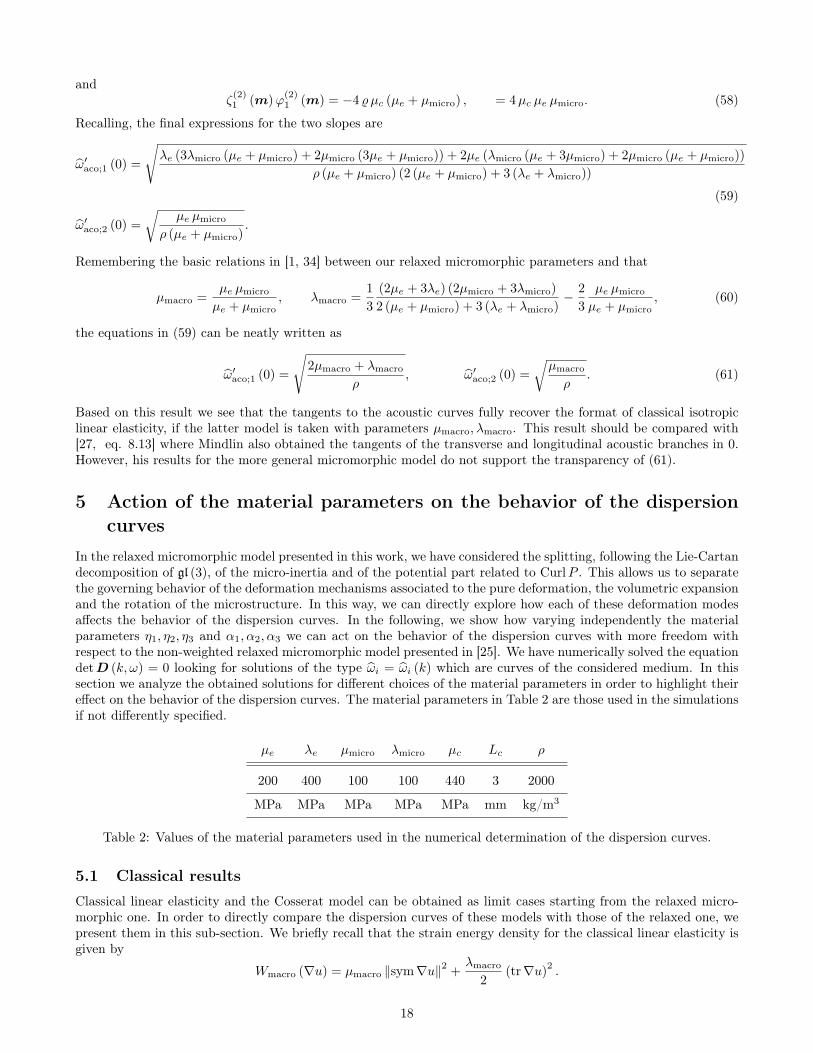
Recalling, the final expressions for the two slopes are

ω′aco;1 (0) =

√λe (3λmicro (µe + µmicro) + 2µmicro (3µe + µmicro)) + 2µe (λmicro (µe + 3µmicro) + 2µmicro (µe + µmicro))

ρ (µe + µmicro) (2 (µe + µmicro) + 3 (λe + λmicro))

(59)

ω′aco;2 (0) =

√µe µmicro

ρ (µe + µmicro).

Remembering the basic relations in [1, 34] between our relaxed micromorphic parameters and that

µmacro =µe µmicro

µe + µmicro, λmacro =

1

3

(2µe + 3λe) (2µmicro + 3λmicro)

2 (µe + µmicro) + 3 (λe + λmicro)− 2

3

µe µmicro

µe + µmicro, (60)

the equations in (59) can be neatly written as

ω′aco;1 (0) =

√2µmacro + λmacro

ρ, ω′aco;2 (0) =

√µmacro

ρ. (61)

Based on this result we see that the tangents to the acoustic curves fully recover the format of classical isotropiclinear elasticity, if the latter model is taken with parameters µmacro, λmacro. This result should be compared with[27, eq. 8.13] where Mindlin also obtained the tangents of the transverse and longitudinal acoustic branches in 0.However, his results for the more general micromorphic model do not support the transparency of (61).

5 Action of the material parameters on the behavior of the dispersioncurves

In the relaxed micromorphic model presented in this work, we have considered the splitting, following the Lie-Cartandecomposition of gl (3), of the micro-inertia and of the potential part related to CurlP . This allows us to separatethe governing behavior of the deformation mechanisms associated to the pure deformation, the volumetric expansionand the rotation of the microstructure. In this way, we can directly explore how each of these deformation modesaffects the behavior of the dispersion curves. In the following, we show how varying independently the materialparameters η1, η2, η3 and α1, α2, α3 we can act on the behavior of the dispersion curves with more freedom withrespect to the non-weighted relaxed micromorphic model presented in [25]. We have numerically solved the equationdetD (k, ω) = 0 looking for solutions of the type ωi = ωi (k) which are curves of the considered medium. In thissection we analyze the obtained solutions for different choices of the material parameters in order to highlight theireffect on the behavior of the dispersion curves. The material parameters in Table 2 are those used in the simulationsif not differently specified.

µe λe µmicro λmicro µc Lc ρ

200 400 100 100 440 3 2000

MPa MPa MPa MPa MPa mm kg/m3

Table 2: Values of the material parameters used in the numerical determination of the dispersion curves.

5.1 Classical resultsClassical linear elasticity and the Cosserat model can be obtained as limit cases starting from the relaxed micro-morphic one. In order to directly compare the dispersion curves of these models with those of the relaxed one, wepresent them in this sub-section. We briefly recall that the strain energy density for the classical linear elasticity isgiven by

Wmacro (∇u) = µmacro ‖sym∇u‖2 +λmacro

2(tr∇u)

2.

18

Moreover, the kinetic energy density used for the classical model is clearly

Jmacro =1

2ρ 〈u,t, u,t〉 .

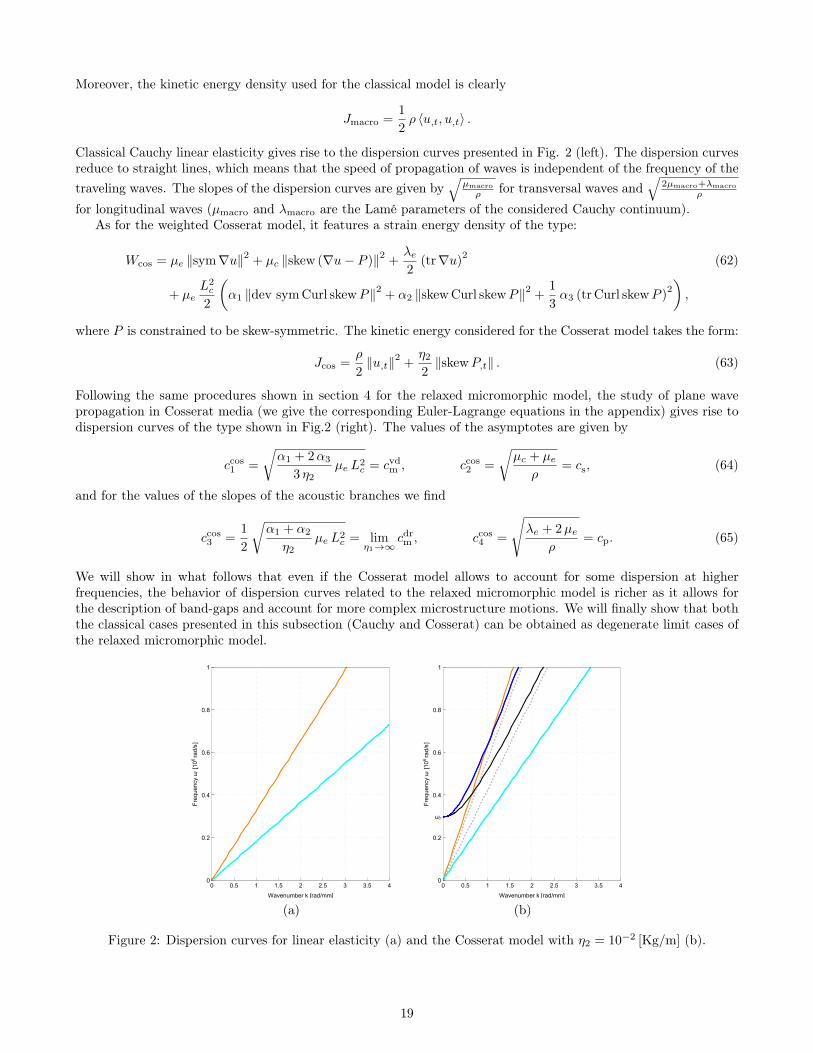
Classical Cauchy linear elasticity gives rise to the dispersion curves presented in Fig. 2 (left). The dispersion curvesreduce to straight lines, which means that the speed of propagation of waves is independent of the frequency of thetraveling waves. The slopes of the dispersion curves are given by

√µmacro

ρ for transversal waves and√

2µmacro+λmacro

ρ

for longitudinal waves (µmacro and λmacro are the Lamé parameters of the considered Cauchy continuum).As for the weighted Cosserat model, it features a strain energy density of the type:

Wcos = µe ‖sym∇u‖2 + µc ‖skew (∇u− P )‖2 +λe2

(tr∇u)2 (62)

+ µeL2c

2

(α1 ‖dev symCurl skewP‖2 + α2 ‖skewCurl skewP‖2 +

1

3α3 (tr Curl skewP )

2

),

where P is constrained to be skew-symmetric. The kinetic energy considered for the Cosserat model takes the form:

Jcos =ρ

2‖u,t‖2 +

η2

2‖skewP,t‖ . (63)

Following the same procedures shown in section 4 for the relaxed micromorphic model, the study of plane wavepropagation in Cosserat media (we give the corresponding Euler-Lagrange equations in the appendix) gives rise todispersion curves of the type shown in Fig.2 (right). The values of the asymptotes are given by

ccos1 =

√α1 + 2α3

3 η2µe L2

c = cvdm , ccos2 =

√µc + µe

ρ= cs, (64)

and for the values of the slopes of the acoustic branches we find

ccos3 =1

2

√α1 + α2

η2µe L2

c = limη1→∞

cdrm , ccos4 =

√λe + 2µe

ρ= cp. (65)

We will show in what follows that even if the Cosserat model allows to account for some dispersion at higherfrequencies, the behavior of dispersion curves related to the relaxed micromorphic model is richer as it allows forthe description of band-gaps and account for more complex microstructure motions. We will finally show that boththe classical cases presented in this subsection (Cauchy and Cosserat) can be obtained as degenerate limit cases ofthe relaxed micromorphic model.

0 0.5 1 1.5 2 2.5 3 3.5 40

0.2

0.4

0.6

0.8

1

Wavenumber k [rad/mm]

Frequency

ω[106rad/s]

0 0.5 1 1.5 2 2.5 3 3.5 40

0.2

0.4

0.6

0.8

ωr

1


Frequency

ω[106rad/s]

(a) (b)

Figure 2: Dispersion curves for linear elasticity (a) and the Cosserat model with η2 = 10−2 [Kg/m] (b).

19

5.2 The classical relaxed micromorphic model and the internal variable modelBefore proceeding, we report some results already available in the literature [25, 26] which we obtain from ourweighted model setting η1 = η2 = η3 and α1 = α2 = α3 (classical relaxed micromorphic case). Moreover, we alsostudy the limit case that is obtained setting α1 = α2 = α3 = 0, which is also known as internal variable model(no derivatives of the micro-distortion P appearing in the strain energy density). The dispersion curves for the twomodels are shown in Fig. 3.

0 0.5 1 1.5 2 2.5 3 3.5 40

0.2

0.4

0.6

0.8

ωl

ωp

ωr

ωs

1


Frequency

ω[106rad/s]

=

= =

μ+λρ

0 0.5 1 1.5 2 2.5 3 3.5 40

0.2

0.4

0.6

0.8

ωp

ωr

ωs

ωt

1


Frequency

ω[106rad/s]

=

= =

μ

ρ

0 0.5 1 1.5 2 2.5 3 3.5 40

0.2

0.4

0.6

0.8

ωp

ωr

ωs

1


Frequency

ω[106rad/s]

=

= =

-

(a1) longitudinal dispersion curves (a2) transversal dispersion curves (a3) uncoupled dispersion curves

0 0.5 1 1.5 2 2.5 3 3.5 40

0.2

0.4

0.6

0.8

ωlint

ωp

ωr

ωs

1


Frequency

ω[106rad/s]

0 0.5 1 1.5 2 2.5 3 3.5 40

0.2

0.4

0.6

0.8

ωp

ωr

ωs

ωtint

1


Frequency

ω[106rad/s]

0 0.5 1 1.5 2 2.5 3 3.5 40

0.2

0.4

0.6

0.8

ωp

ωr

ωs

1


Frequency

ω[106rad/s]

(b1) longitudinal dispersion curves (b2) transversal dispersion curves (b3) uncoupled dispersion curves

Figure 3: Dispersion curves for the classical relaxed micromorphic case α1 = α2 = α3 = 1 and η1 = η2 = η3 =10−2Kg/m (a1,a2,a3), and for the internal variable case: α1 = α2 = α3 = 0 and η1 = η2 = η3 = 10−2Kg/m(b1,b2,b3).

In both cases, we find 8 different dispersion curves instead of 12. Indeed, we would expect 12 curves since thekinematics is given by the 3 components of the displacement field u, plus the 9 components of the micro-distortionfield P . This means that there are overlapped curves (our check exhibits 4 couples of overlapping curves). Theband-gap region is clearly present in both models. These results are fully compatible with what has been found in[25] and in [26]. In particular, we find the same behavior presented in [25] and [26], where sufficient conditions onthe constitutive parameters have been found that guarantee the existence of band gaps. Moreover, for the internal-variable case, it has been shown in [26] that two optic branches become horizontal and four horizontal asymptotescan be found which are not related with the two horizontal asymptotes of the case α1 = α2 = α3 6= 0.

In the present work, in order to present a parametric study on the behavior of the dispersion curves varying agreat number of material parameters, we have decided to represent, in the newly studied cases, all the dispersion

20

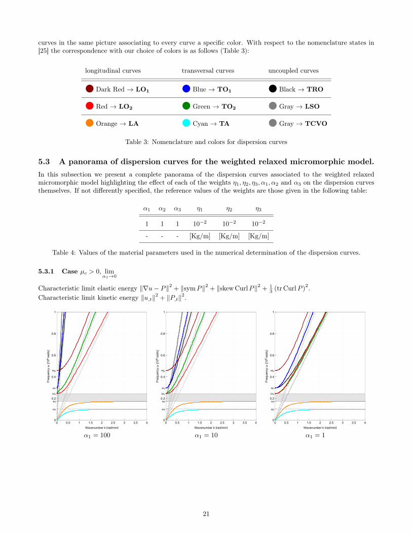
curves in the same picture associating to every curve a specific color. With respect to the nomenclature states in[25] the correspondence with our choice of colors is as follows (Table 3):

longitudinal curves transversal curves uncoupled curves

Dark Red → LO1 Blue → TO1 Black → TRO

Red → LO2 Green → TO2 Gray → LSO

Orange → LA Cyan → TA Gray → TCVO

Table 3: Nomenclature and colors for dispersion curves

5.3 A panorama of dispersion curves for the weighted relaxed micromorphic model.In this subsection we present a complete panorama of the dispersion curves associated to the weighted relaxedmicromorphic model highlighting the effect of each of the weights η1, η2, η3, α1, α2 and α3 on the dispersion curvesthemselves. If not differently specified, the reference values of the weights are those given in the following table:

α1 α2 α3 η1 η2 η3

1 1 1 10−2 10−2 10−2

- - - [Kg/m] [Kg/m] [Kg/m]

Table 4: Values of the material parameters used in the numerical determination of the dispersion curves.

5.3.1 Case µc > 0, limα1→0

Characteristic limit elastic energy ‖∇u− P‖2 + ‖symP‖2 + ‖skewCurlP‖2 + 13 (tr CurlP )

2.Characteristic limit kinetic energy ‖u,t‖2 + ‖P,t‖2.

0 0.5 1 1.5 2 2.5 3 3.5 40

0.2

0.4

0.6

0.8

ωl

ωp

ωr

ωs

ωt

1


Frequency

ω[106rad/s]

0 0.5 1 1.5 2 2.5 3 3.5 40

0.2

0.4

0.6

0.8

ωl

ωp

ωr

ωs

ωt

1


Frequency

ω[106rad/s]

0 0.5 1 1.5 2 2.5 3 3.5 40

0.2

0.4

0.6

0.8

ωl

ωp

ωr

ωs

ωt

1


Frequency

ω[106rad/s]

α1 = 100 α1 = 10 α1 = 1

21

0 0.5 1 1.5 2 2.5 3 3.5 40

0.2

0.4

0.6

0.8

ωl

ωp

ωr

ωs

ωt

1


Frequency

ω[106rad/s]

0 0.5 1 1.5 2 2.5 3 3.5 40

0.2

0.4

0.6

0.8

ωl

ωp

ωr

ωs

ωt

1

Wavenumber k [rad/mm]Frequency

ω[106rad/s]

0 0.5 1 1.5 2 2.5 3 3.5 40

0.2

0.4

0.6

0.8

ωl

ωp

ωr

ωs

ωt

1


Frequency

ω[106rad/s]

α1 = 0.05 α1 = 0.01 α1 = 0

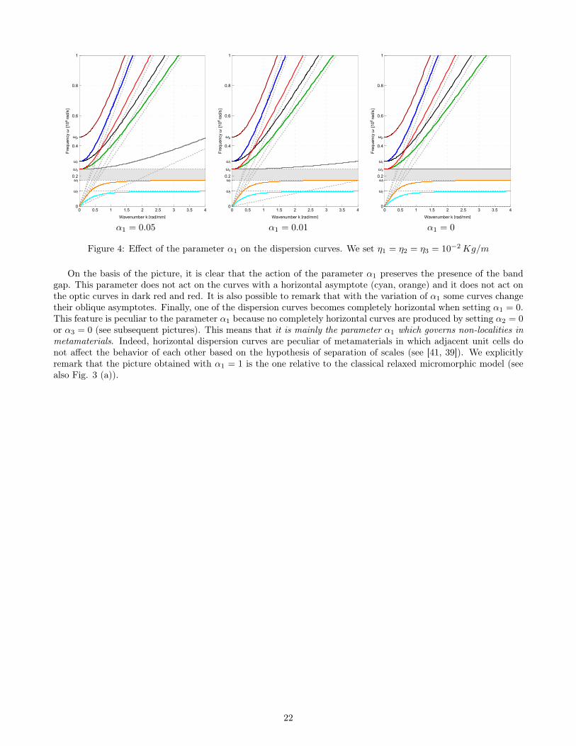
Figure 4: Effect of the parameter α1 on the dispersion curves. We set η1 = η2 = η3 = 10−2Kg/m

On the basis of the picture, it is clear that the action of the parameter α1 preserves the presence of the bandgap. This parameter does not act on the curves with a horizontal asymptote (cyan, orange) and it does not act onthe optic curves in dark red and red. It is also possible to remark that with the variation of α1 some curves changetheir oblique asymptotes. Finally, one of the dispersion curves becomes completely horizontal when setting α1 = 0.This feature is peculiar to the parameter α1 because no completely horizontal curves are produced by setting α2 = 0or α3 = 0 (see subsequent pictures). This means that it is mainly the parameter α1 which governs non-localities inmetamaterials. Indeed, horizontal dispersion curves are peculiar of metamaterials in which adjacent unit cells donot affect the behavior of each other based on the hypothesis of separation of scales (see [41, 39]). We explicitlyremark that the picture obtained with α1 = 1 is the one relative to the classical relaxed micromorphic model (seealso Fig. 3 (a)).

22

5.3.2 Case µc > 0, limα2→0

Characteristic limit elastic energy ‖∇u− P‖2 + ‖symP‖2 + ‖symCurlP‖2.Characteristic limit kinetic energy ‖u,t‖2 + ‖P,t‖2.

0 0.5 1 1.5 2 2.5 3 3.5 40

0.2

0.4

0.6

0.8

ωl

ωp

ωr

ωs

ωt

1


Frequency

ω[106rad/s]

0 0.5 1 1.5 2 2.5 3 3.5 40

0.2

0.4

0.6

0.8

ωl

ωp

ωr

ωs

ωt

1


Frequency

ω[106rad/s]

0 0.5 1 1.5 2 2.5 3 3.5 40

0.2

0.4

0.6

0.8

ωl

ωp

ωr

ωs

ωt

1


Frequency

ω[106rad/s]

α2 = 100 α2 = 10 α2 = 1

0 0.5 1 1.5 2 2.5 3 3.5 40

0.2

0.4

0.6

0.8

ωl

ωp

ωr

ωs

ωt

1


Frequency

ω[106rad/s]

0 0.5 1 1.5 2 2.5 3 3.5 40

0.2

0.4

0.6

0.8

ωl

ωp

ωr

ωs

ωt

1


Frequency

ω[106rad/s]

0 0.5 1 1.5 2 2.5 3 3.5 40

0.2

0.4

0.6

0.8

ω1

ω2

ωp

ωr

ωs

ωt

1


Frequency

ω[106rad/s]

α2 = 0.05 α2 = 0.01 α2 = 0

Figure 5: Effect of the parameter α2 on the dispersion curves.

On the basis of the picture, it is clear that the action of the parameter α2 preserves the presence of the bandgap. Varying the values of this parameter, we have an action only on the curves in black and gray. The parameterα2 is also seen to have some direct influence on the horizontal asymptotes for the orange optic wave. In fact ifα2 = 0 the value of this horizontal asymptote changes and we can calculate it solving the equation

c16

(ω2∗)

= 0 (66)

with respect to ω∗. This is exactly the direct application of the proposition 4 in the case in which the coefficientc18

(ω2)is not present. Between the solutions of the eq.(66) we find

ω1 =

√√√√ q1

3η1η3 (λe + 2µe)−

√(q2)

2 − 4 (3η1η3λe + 6η1η3µe) q3

6η1η3 (λe + 2µe)+

9η1λeλh6η1η3 (λe + 2µe)

ω2 =

√√√√ q1

3η1η3 (λe + 2µe)+

√(q2)

2 − 4 (3η1η3λe + 6η1η3µe) q3

6η1η3 (λe + 2µe)+

9η1λeλh6η1η3 (λe + 2µe)

23

where

q1 = 4η1µ2e + 2η3µ

2e + 6η1λeµe + 3η3λeµe + 6η1µeµmicro + 6η3µeµmicro + 9η1µeλh + 3η1λeµmicro + 3η3λeµmicro

q2 = −12η1λeµe − 6η3λeµe − 8η1µ2e − 4η3µ

2e − 18η1µeλmicro − 6η1λeµmicro − 6η3λeµmicroµmicro

− 9η1λeλmicro − 12η1µeµmicro − 12η3µe,

q3 = 12µ2eλmicro + 18λeµeλmicro + 36λeµeµmicro + 36µeλhµmicro + 12λeµ

2micro

+ 18λeλmicroµmicro + 24µ2eµmicro + 24µeµ

2micro.

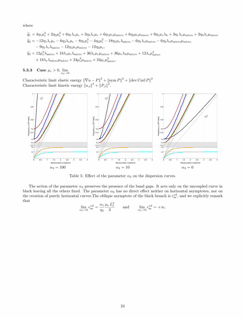
5.3.3 Case µc > 0, limα3→0

Characteristic limit elastic energy ‖∇u− P‖2 + ‖symP‖2 + ‖devCurlP‖2

Characteristic limit kinetic energy ‖u,t‖2 + ‖P,t‖2.

0 0.5 1 1.5 2 2.5 3 3.5 4

0.2

0.4

0.6

0.8

ωl

ωp

ωr

ωs

ωt

1


Frequency

ω[106rad/s]

0 0.5 1 1.5 2 2.5 3 3.5 4

0.2

0.4

0.6

0.8

ωl

ωp

ωr

ωs

ωt

1


Frequency

ω[106rad/s]

0 0.5 1 1.5 2 2.5 3 3.5 4

0.2

0.4

0.6

0.8

ωl

ωp

ωr

ωs

ωt

1


Frequency

ω[106rad/s]

α3 = 100 α3 = 10 α3 = 0

Table 5: Effect of the parameter α3 on the dispersion curves.

The action of the parameter α3 preserves the presence of the band gaps. It acts only on the uncoupled curve inblack leaving all the others fixed. The parameter α3 has no direct effect neither on horizontal asymptotes, nor onthe creation of purely horizontal curves.The oblique asymptote of the black branch is cvd

m , and we explicitly remarkthat

limα3→0

cvdm =

α1

η3

µe L2c

3and lim

α3→0cvdm = +∞.

24

5.3.4 Case µc > 0, limα2,α3→0

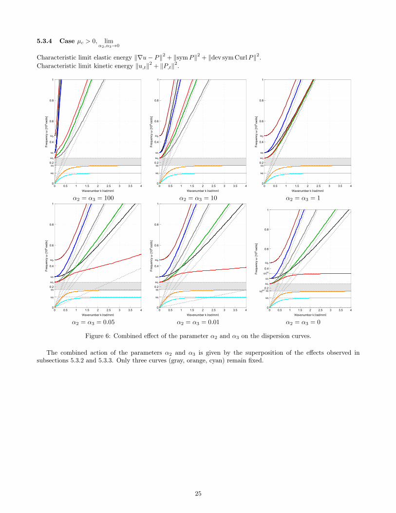
Characteristic limit elastic energy ‖∇u− P‖2 + ‖symP‖2 + ‖dev symCurlP‖2.Characteristic limit kinetic energy ‖u,t‖2 + ‖P,t‖2.

0 0.5 1 1.5 2 2.5 3 3.5 40

0.2

0.4

0.6

0.8

ωl

ωp

ωr

ωs

ωt

1


Frequency

ω[106rad/s]

0 0.5 1 1.5 2 2.5 3 3.5 40

0.2

0.4

0.6

0.8

ωl

ωp

ωr

ωs

ωt

1


Frequency

ω[106rad/s]

0 0.5 1 1.5 2 2.5 3 3.5 40

0.2

0.4

0.6

0.8

ωl

ωp

ωr

ωs

ωt

1


Frequency

ω[106rad/s]

α2 = α3 = 100 α2 = α3 = 10 α2 = α3 = 1

0 0.5 1 1.5 2 2.5 3 3.5 40

0.2

0.4

0.6

0.8

ωl

ωp

ωr

ωs

ωt

1


Frequency

ω[106rad/s]

0 0.5 1 1.5 2 2.5 3 3.5 40

0.2

0.4

0.6

0.8

ωl

ωp

ωr

ωs

ωt

1


Frequency

ω[106rad/s]

0 0.5 1 1.5 2 2.5 3 3.5 40

0.2

0.4

0.6

0.8

ωlint

ω1int

ωl

ωp

ωr

ωs

ωt

1


Frequency

ω[106rad/s]

α2 = α3 = 0.05 α2 = α3 = 0.01 α2 = α3 = 0

Figure 6: Combined effect of the parameter α2 and α3 on the dispersion curves.

The combined action of the parameters α2 and α3 is given by the superposition of the effects observed insubsections 5.3.2 and 5.3.3. Only three curves (gray, orange, cyan) remain fixed.

25

5.3.5 Vanishing Cosserat couple modulus µc = 0 and limα1→0

Characteristic limit elastic energy ‖sym (∇u− P )‖2 + ‖symP‖2 + ‖skewCurlP‖2 + 13 (tr CurlP )

2.

Characteristic limit kinetic energy ‖u,t‖2 + ‖P,t‖2.

0 0.5 1 1.5 2 2.5 3 3.5 4

0.2

0.4

0.6

0.8

ωl

ωp

ωr

ωs

ωt

1


Frequency

ω[106rad/s]

0 0.5 1 1.5 2 2.5 3 3.5 4

0.2

0.4

0.6

0.8

ωl

ωp

ωr

ωs

ωt

1


Frequency

ω[106rad/s]

0 0.5 1 1.5 2 2.5 3 3.5 4

0.2

0.4

0.6

0.8

ωl

ωp

ωr

ωs

ωt

1


Frequency

ω[106rad/s]

α1 = 100 α1 = 10 α1 = 1

0 0.5 1 1.5 2 2.5 3 3.5 4

0.2

0.4

0.6

0.8

ωl

ωp

ωr

ωs

ωt

1


Frequency

ω[106rad/s]

0 0.5 1 1.5 2 2.5 3 3.5 4

0.2

0.4

0.6

0.8

ωl

ωp

ωr

ωs

ωt

1


Frequency

ω[106rad/s]

0 0.5 1 1.5 2 2.5 3 3.5 4

0.2

0.4

0.6

0.8

ωl

ωp

ωr

ωs

ωt

1


Frequency

ω[106rad/s]

α1 = 0.05 α1 = 0.01 α1 = 0

Figure 7: Effect of the parameter α1 on the dispersion curves for the case µc = 0. Higher values of α1 have somenon-negligible effects on the new extra acoustic curves.

In this case we see that two curves (black and green) become acoustic. As a consequence, there is no completeband gap. This is coherent with the results of [25] in which the existence of 2 complete band-gaps is directly relatedto a non-vanishing Cosserat couple modulus µc > 0. The particular effect of the parameter α1 = 0 on the existenceof a horizontal curve is preserved (see also Fig.4).

We explicitly mention that the presence of 4 acoustic curves is not observed in any known pattern of dispersioncurves for real metamaterials. This means that such metamaterials need to have a non-vanishing Cosserat couplemodulus µc > 0 which allows for the description of rotational micro-motions at higher frequencies.

26


Characteristic limit elastic energy ‖sym (∇u− P )‖2 + ‖symP‖2 + ‖symCurlP‖2.Characteristic limit kinetic energy ‖u,t‖2 + ‖P,t‖2.

0 0.5 1 1.5 2 2.5 3 3.5 4

0.2

0.4

0.6

0.8

ωl

ωp

ωr

ωs

ωt

1


Frequency

ω[106rad/s]

0 0.5 1 1.5 2 2.5 3 3.5 4

0.2

0.4

0.6

0.8

ωl

ωp

ωr

ωs

ωt

1


Frequency

ω[106rad/s]

0 0.5 1 1.5 2 2.5 3 3.5 4

0.2

0.4

0.6

0.8

ωl

ωp

ωr

ωs

ωt

1


Frequency

ω[106rad/s]

α2 = 100 α2 = 10 α2 = 1

0 0.5 1 1.5 2 2.5 3 3.5 4

0.2

0.4

0.6

0.8

ωl

ωp

ωr

ωs

ωt

1


Frequency

ω[106rad/s]

0 0.5 1 1.5 2 2.5 3 3.5 4

0.2

0.4

0.6

0.8

ωl

ωp

ωr

ωs

ωt

1


Frequency

ω[106rad/s]

0 0.5 1 1.5 2 2.5 3 3.5 4

0.2

0.4

0.6

0.8

ω1

ω2

ωp

ωr

ωs

ωt

1


Frequency

ω[106rad/s]

α2 = 0.05 α2 = 0.01 α2 = 0

Figure 8: Effect of the parameter α2 on the dispersion curves for the case µc = 0.

Again, the two extra characteristic acoustic curves that arise when setting µc = 0 are recovered again. An effectof the parameter α2 similar to the one shown in Fig. 5 is also found for the optic wave which becomes horizontal.A high value of α2 has also a visible effect on one of the two extra acoustic curves.

27


Characteristic limit elastic energy ‖sym (∇u− P )‖2 + ‖symP‖2 + ‖devCurlP‖2.Characteristic limit kinetic energy ‖u,t‖2 + ‖P,t‖2.

0 0.5 1 1.5 2 2.5 3 3.5 4

0.2

0.4

0.6

0.8

ωl

ωp

ωr

ωs

ωt

1


Frequency

ω[106rad/s]

0 0.5 1 1.5 2 2.5 3 3.5 4

0.2

0.4

0.6

0.8

ωl

ωp

ωr

ωs

ωt

1


Frequency

ω[106rad/s]

0 0.5 1 1.5 2 2.5 3 3.5 4

0.2

0.4

0.6

0.8

ωl

ωp

ωr

ωs

ωt

1


Frequency

ω[106rad/s]

α3 = 100 α3 = 10 α3 = 0

Table 6: Effect of the parameter α3 on the dispersion curves for the case µc = 0.

In this case we see again that two curves (blue and black) become acoustic. There is no complete band gap. Thisconfirms once again the need of having µc > 0 as a necessary condition for the existence of complete band-gaps.The effect of the parameter α3 is limited to the control of the slope of one of the two extra acoustic curves whoseonset is related to the fact of setting µc = 0.

28

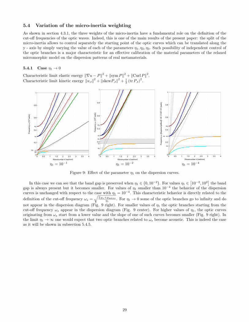
5.4 Variation of the micro-inertia weightingAs shown in section 4.3.1, the three weights of the micro-inertia have a fundamental role on the definition of thecut-off frequencies of the optic waves. Indeed, this is one of the main results of the present paper: the split of themicro-inertia allows to control separately the starting point of the optic curves which can be translated along they - axis by simply varying the value of each of the parameters η1, η2, η3. Such possibility of independent control ofthe optic branches is a major characteristic for an effective calibration of the material parameters of the relaxedmicromorphic model on the dispersion patterns of real metamaterials.

5.4.1 Case η1 → 0

Characteristic limit elastic energy ‖∇u− P‖2 + ‖symP‖2 + ‖CurlP‖2.Characteristic limit kinetic energy ‖u,t‖2 + ‖skewP,t‖2 + 1

3 (trP,t)2.

0 0.5 1 1.5 2 2.5 3 3.5 40

0.2

0.4

0.6

0.8

ωl

ωp

ωr

ωs

ωt

1


Frequency

ω[106rad/s]

0 0.5 1 1.5 2 2.5 3 3.5 40

0.2

0.4

0.6

0.8

ωl

ωp

ωr

ωs

ωt

1


Frequency

ω[106rad/s]

0 0.5 1 1.5 2 2.5 3 3.5 40

0.2

0.4

0.6

0.8

ωl

ωp

ωr

ωt

1


ω[SuperscriptBox

[\(10\),\(\(6\)\(\\)\)]rad/s]

η1 = 10−1 η1 = 10−2 η1 = 10−4

Figure 9: Effect of the parameter η1 on the dispersion curves.

In this case we can see that the band gap is preserved when η1 ∈(0, 10−2

). For values η1 ∈

[10−2, 102

]the band

gap is always present but it becomes smaller. For values of η1 smaller than 10−4 the behavior of the dispersioncurves is unchanged with respect to the case with η1 = 10−4. This characteristic behavior is directly related to thedefinition of the cut-off frequency ωs =

√2µe+µmicro

η1. For η1 → 0 some of the optic branches go to infinity and do

not appear in the dispersion diagram (Fig. 9 right). For smaller values of η1 the optic branches starting from thecut-off frequency ωs appear in the dispersion diagram (Fig. 9 center). For higher values of η1, the optic curvesoriginating from ωs start from a lower value and the slope of one of such curves becomes smaller (Fig. 9 right). Inthe limit η1 →∞ one would expect that two optic branches related to ωs become acoustic. This is indeed the caseas it will be shown in subsection 5.4.5.

29

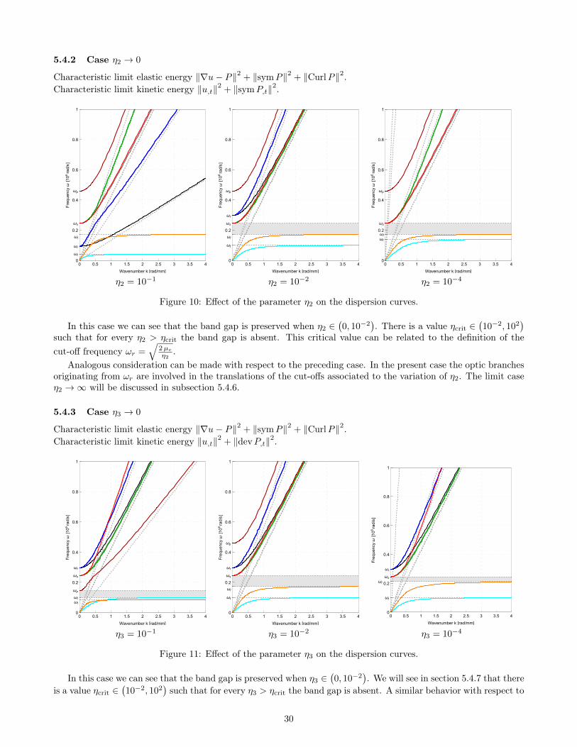
5.4.2 Case η2 → 0

Characteristic limit elastic energy ‖∇u− P‖2 + ‖symP‖2 + ‖CurlP‖2.Characteristic limit kinetic energy ‖u,t‖2 + ‖symP,t‖2.

0 0.5 1 1.5 2 2.5 3 3.5 40

0.2

0.4

0.6

0.8

ωl

ωp

ωr

ωs

ωt

1


Frequency

ω[106rad/s]

0 0.5 1 1.5 2 2.5 3 3.5 40

0.2

0.4

0.6

0.8

ωl

ωp

ωr

ωs

ωt

1


Frequency

ω[106rad/s]

0 0.5 1 1.5 2 2.5 3 3.5 40

0.2

0.4

0.6

0.8

ωl

ωp

ωs

ωt

1


Frequency

ω[106rad/s]

η2 = 10−1 η2 = 10−2 η2 = 10−4



). There is a value ηcrit ∈

(10−2, 102

)such that for every η2 > ηcrit the band gap is absent. This critical value can be related to the definition of thecut-off frequency ωr =

√2µcη2

.Analogous consideration can be made with respect to the preceding case. In the present case the optic branches

originating from ωr are involved in the translations of the cut-offs associated to the variation of η2. The limit caseη2 →∞ will be discussed in subsection 5.4.6.

5.4.3 Case η3 → 0

Characteristic limit elastic energy ‖∇u− P‖2 + ‖symP‖2 + ‖CurlP‖2.Characteristic limit kinetic energy ‖u,t‖2 + ‖devP,t‖2.

0 0.5 1 1.5 2 2.5 3 3.5 40

0.2

0.4

0.6

0.8

ωl

ωp

ωr

ωs

ωt

1


Frequency

ω[106rad/s]

0 0.5 1 1.5 2 2.5 3 3.5 40

0.2

0.4

0.6

0.8

ωl

ωp

ωr

ωs

ωt

1


Frequency

ω[106rad/s]

0 0.5 1 1.5 2 2.5 3 3.5 40

0.2

0.4

0.6

0.8

ωl

ωr

ωs

ωt

1


Frequency

ω[106rad/s]

η3 = 10−1 η3 = 10−2 η3 = 10−4



). We will see in section 5.4.7 that there

is a value ηcrit ∈(10−2, 102

)such that for every η3 > ηcrit the band gap is absent. A similar behavior with respect to

30

the previous two cases is observed for what concerns the optic wave originating from ωp =√

3(λe+λmicro)+2(µe+µmicro)η3

.The limit case η3 →∞ will be described in section 5.4.7.

5.4.4 Cases η1,η2, η3 → 0: the fundamental role of the micro-inertia for enriched continuum mechan-ics

Characteristic limit elastic energy ‖∇u− P‖2 + ‖symP‖2 + ‖CurlP‖2.Characteristic limit kinetic energy ‖u,t‖2.

0 0.5 1 1.5 2 2.5 3 3.5 40

0.2

0.4

0.6

0.8

ωl

ωp

ωr ωs

ωt

1


Frequency

ω[106rad/s]

0 0.5 1 1.5 2 2.5 3 3.5 40

0.2

0.4

0.6

0.8

ωl

ωp

ωr

ωs

ωt

1


Frequency

ω[106rad/s]

0 0.5 1 1.5 2 2.5 3 3.5 40

0.2

0.4

0.6

0.8

ωl

ωp

ωr

ωs

ωt

1


Frequency

ω[106rad/s]

η1 = η2 = η3 = 10−1 η1 = η2 = η3 = 10−2 η1 = η2 = η3 = 5 · 10−3

0 0.5 1 1.5 2 2.5 3 3.5 40

0.2

0.4

0.6

0.8

ωl

ωr

ωs

ωt

1


Frequency

ω[106rad/s]

0 0.5 1 1.5 2 2.5 3 3.5 40

0.2

0.4

0.6

0.8

ωt1


Frequency

ω[106rad/s]

0 0.5 1 1.5 2 2.5 3 3.5 40

0.2

0.4

0.6

0.8

1


Frequency

ω[106rad/s]

η1 = η2 = η3 = 10−3 η1 = η2 = η3 = 10−4 η1 = η2 = η3 = 10−5

Figure 12: Combined effect of the parameter η1, η2, η3 on the dispersion curves.

In Figure 12 we show the combined effect of the micro-inertia parameters on the behavior of the dispersion curves.When letting the three parameters tend to zero with the same speed, one ends up with a dispersion diagram whichis peculiar of the classical linear elastic Cauchy media (Fig.12 bottom right).

This is a fundamental result of the present study which is not exhaustively treated in the literature: if oneconsiders a continuum with enriched kinematic (u, P ), if no micro-inertia is considered to complement the macro-inertia ρ ‖u,t‖2, then the dispersion curves will not be different from those of the classical Cauchy continuum (Fig.2 (a)). In order to activate the micro-motions associated to the micro-distortion tensor P a micro-inertia η ‖P,t‖2is needed.

31

5.4.5 Case η1 → +∞

Characteristic limit elastic energy ‖sym (∇u− P )‖2 + ‖symP‖2 + ‖CurlP‖2.Characteristic limit kinetic energy ‖u,t‖2 + ‖skewP,t‖2 + 1

3 (trP,t)2, dev symP,t = 0.

0 0.5 1 1.5 2 2.5 3 3.5 4

0.2

0.4

0.6

0.8

ωl

ωp

ωr

ωsωt

1


Frequency

ω[106rad/s]

0 0.5 1 1.5 2 2.5 3 3.5 4

0.2

0.4

0.6

0.8

ωl

ωp

ωr

ωsωt

1


Frequency

ω[106rad/s]

0 0.5 1 1.5 2 2.5 3 3.5 4

0.2

0.4

0.6

0.8

ωl

ωp

ωr

ωsωt

1


Frequency

ω[106rad/s]

η1 = 10 η1 = 103 η1 = 105


We complete here the case treated in subsection 3.4.1, by describing the behavior of the dispersion curves whenletting η1 →∞.

As expected, the optic branches originating from the cut-off ωs become acoustic and, moreover, they are non-dispersive. What is more surprising is that the original acoustic branches flatten to zero and hence disappear fromthe dispersion diagram.

This means that, in the limit, we are constraining the system to have less degrees of freedom by artificiallyimposing an infinite inertia that does not allow some specific micro-vibrations.

0 0.5 1 1.5 2 2.5 3 3.5 40

0.01

0.02

0.03

0.04

0.05

ωlωs

ωt


Frequency

ω[106rad/s]

0 0.5 1 1.5 2 2.5 3 3.5 40

0.001

0.002

ωl

ωs

ωt


Frequency

ω[106rad/s]

0 0.5 1 1.5 2 2.5 3 3.5 40

0.0001

0.0002

ωl

ωs

ωt


Frequency

ω[106rad/s]

η1 = 101 η1 = 103 η1 = 105

Figure 14: Zoom on the acoustic branches.

In Fig. 14 we make a zoom on the acoustic curves that are flattening to zero.

32

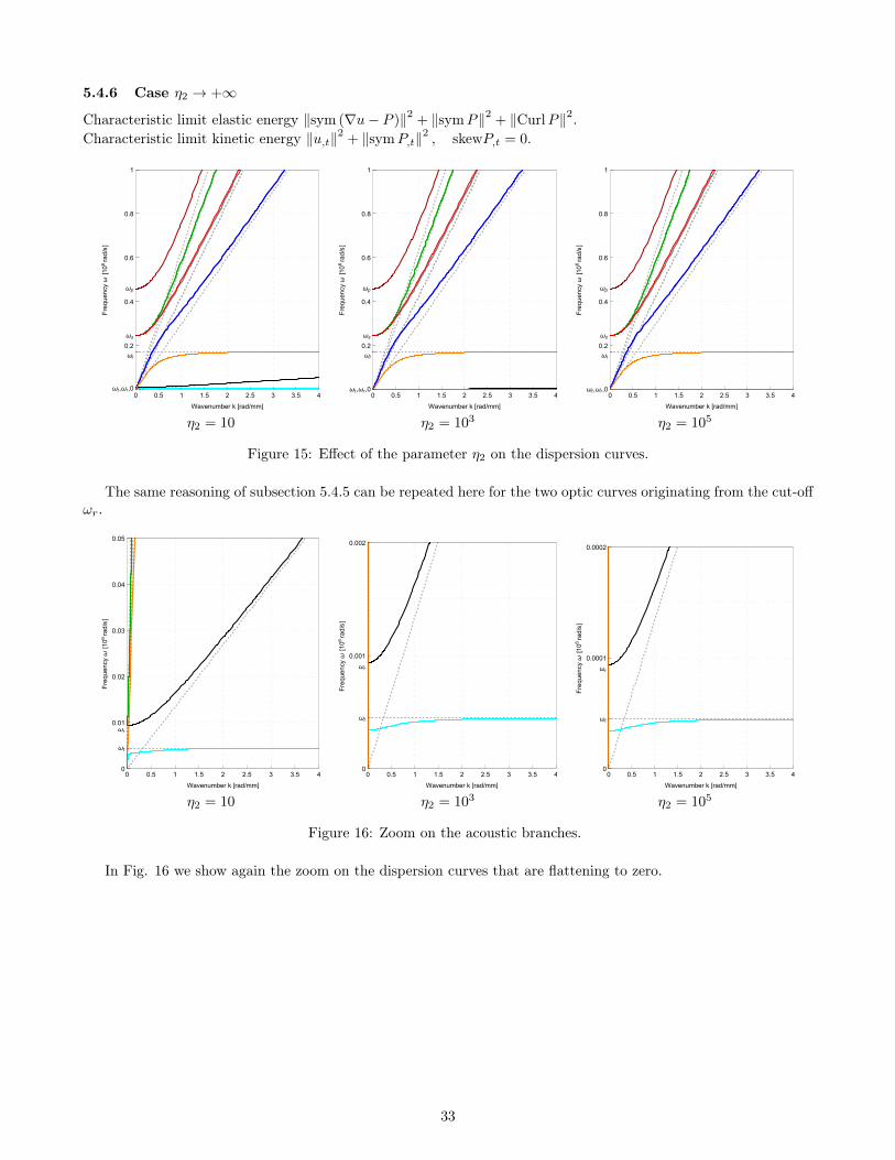
5.4.6 Case η2 → +∞

Characteristic limit elastic energy ‖sym (∇u− P )‖2 + ‖symP‖2 + ‖CurlP‖2.Characteristic limit kinetic energy ‖u,t‖2 + ‖symP,t‖2 , skewP,t = 0.

0 0.5 1 1.5 2 2.5 3 3.5 4

0.2

0.4

0.6

0.8

ωl

ωp

ωs

ωt ,ωr,0

1


Frequency

ω[106rad/s]

0 0.5 1 1.5 2 2.5 3 3.5 4

0.2

0.4

0.6

0.8

ωl

ωp

ωs

ωt ,ωr,0

1


Frequency

ω[106rad/s]

0 0.5 1 1.5 2 2.5 3 3.5 4

0.2

0.4

0.6

0.8

ωl

ωp

ωs

ωt ,ωr,0

1


Frequency

ω[106rad/s]

η2 = 10 η2 = 103 η2 = 105


The same reasoning of subsection 5.4.5 can be repeated here for the two optic curves originating from the cut-offωr.

0 0.5 1 1.5 2 2.5 3 3.5 40

0.01

0.02

0.03

0.04

0.05

ωr

ωt


Frequency

ω[106rad/s]

0 0.5 1 1.5 2 2.5 3 3.5 40

0.001

0.002

ωr

ωt


Frequency

ω[106rad/s]

0 0.5 1 1.5 2 2.5 3 3.5 40

0.0001

0.0002

ωr

ωt


Frequency

ω[106rad/s]

η2 = 10 η2 = 103 η2 = 105


In Fig. 16 we show again the zoom on the dispersion curves that are flattening to zero.

33

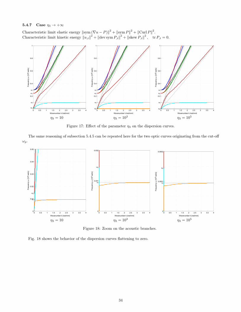
5.4.7 Case η3 → +∞

Characteristic limit elastic energy ‖sym (∇u− P )‖2 + ‖symP‖2 + ‖CurlP‖2.Characteristic limit kinetic energy ‖u,t‖2 + ‖dev symP,t‖2 + ‖skewP,t‖2 , trP,t = 0.

0 0.5 1 1.5 2 2.5 3 3.5 4

0.2

0.4

0.6

0.8

ωp

ωr

ωs

ωt

1


Frequency

ω[106rad/s]

0 0.5 1 1.5 2 2.5 3 3.5 4

0.2

0.4

0.6

0.8

ωp

ωr

ωs

ωt

1


Frequency

ω[106rad/s]

0 0.5 1 1.5 2 2.5 3 3.5 4

0.2

0.4

0.6

0.8

ωp

ωr

ωs

ωt

1


Frequency

ω[106rad/s]

η3 = 10 η3 = 103 η3 = 105


The same reasoning of subsection 5.4.5 can be repeated here for the two optic curves originating from the cut-offωp.

0 0.5 1 1.5 2 2.5 3 3.5 40

0.01

0.02

0.03

0.04

0.05

ωl

ωp


Frequency

ω[106rad/s]

0 0.5 1 1.5 2 2.5 3 3.5 40

0.001

0.002

ωl

ωp


Frequency

ω[106rad/s]

0 0.5 1 1.5 2 2.5 3 3.5 40

0.0001

0.0002

ωl

ωp


Frequency

ω[106rad/s]

η3 = 10 η3 = 103 η3 = 105


Fig. 18 shows the behavior of the dispersion curves flattening to zero.

34

5.4.8 Cases η1,η2, η3 → +∞: a rigidified Cauchy material

Characteristic limit elastic energy ‖sym (∇u− P )‖2 + ‖symP‖2 + ‖devCurlP‖2.Characteristic limit kinetic energy ‖u,t‖2 , P,t = 0.

0 0.5 1 1.5 2 2.5 3 3.5 40

0.2

0.4

0.6

0.8

1


Frequency

ω[106rad/s]

0 0.5 1 1.5 2 2.5 3 3.5 40

0.2

0.4

0.6

0.8

1


Frequency

ω[106rad/s]

0 0.5 1 1.5 2 2.5 3 3.5 40

0.2

0.4

0.6

0.8

1


Frequency

ω[106rad/s]

η1 = η2 = η3 = 10 η1 = η2 = η3 = 103 η1 = η2 = η3 = 105

Figure 19: Combined effect of the parameters η1, η2η3 → 0 on the dispersion curves.

This particular case, obtained letting simultaneously η1, η2 and η3 tend to infinity, gives rise to a Cauchy-likematerial behavior. Nevertheless, the physical meaning attached to this phenomenon is drastically different from theresult obtained in section 5.4.4 when setting η1 = η2 = η3 = 0.

Indeed, in that case, considering an enriched kinematics (u, P ) without the micro-inertia ‖P,t‖2 did not allow tosuch microstructure to manifest itself. It is as if one introduces a complex constitutive behavior for a metamaterial,but does not allow to investigate its dynamical behavior. Indeed, the result was the same obtained for the classicalCauchy medium as if it did not have any underlying microstructure.

On the other hand, the case considered here is quite different: we are indeed introducing the inertia of themicrostructure in the model, but such inertia is so high that the microstructure is “frozen” and cannot vibratelocally. We thus end-up with a Cauchy material which is more rigid than the original one (slope of the acousticcurves is bigger than that in Fig. 1(a)).

35

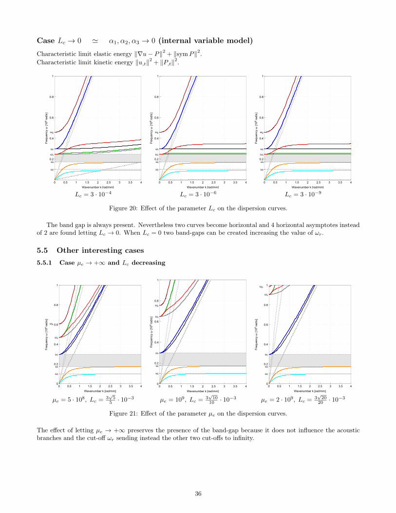
Case Lc → 0 ' α1, α2, α3 → 0 (internal variable model)

Characteristic limit elastic energy ‖∇u− P‖2 + ‖symP‖2.Characteristic limit kinetic energy ‖u,t‖2 + ‖P,t‖2.

0 0.5 1 1.5 2 2.5 3 3.5 4

0.2

0.4

0.6

0.8

ωl

ωp

ωr

ωs

ωt

1


Frequency

ω[106rad/s]

0 0.5 1 1.5 2 2.5 3 3.5 4

0.2

0.4

0.6

0.8

ωl

ωp

ωr

ωs

ωt

1


Frequency

ω[106rad/s]

0 0.5 1 1.5 2 2.5 3 3.5 4

0.2

0.4

0.6

0.8

ωl

ωp

ωr

ωs

ωt

1


Frequency

ω[106rad/s]

Lc = 3 · 10−4 Lc = 3 · 10−6 Lc = 3 · 10−9

Figure 20: Effect of the parameter Lc on the dispersion curves.

The band gap is always present. Nevertheless two curves become horizontal and 4 horizontal asymptotes insteadof 2 are found letting Lc → 0. When Lc = 0 two band-gaps can be created increasing the value of ωr.

5.5 Other interesting cases5.5.1 Case µe → +∞ and Lc decreasing

0 0.5 1 1.5 2 2.5 3 3.5 40

0.2

0.4

0.6

0.8

ωl

ωp

ωr

ωs

ωt

1


Frequency

ω[106rad/s]

0 0.5 1 1.5 2 2.5 3 3.5 40

0.2

0.4

0.6

0.8

ωl

ωp

ωr

ωs

ωt

1


Frequency

ω[106rad/s]

0 0.5 1 1.5 2 2.5 3 3.5 40

0.2

0.4

0.6

0.8

ωl

ωp

ωr

ωs

ωt

1


Frequency

ω[106rad/s]

µe = 5 · 108, Lc = 3√

55 · 10−3 µe = 109, Lc = 3

√10

10 · 10−3 µe = 2 · 109, Lc = 3√

2020 · 10−3

Figure 21: Effect of the parameter µe on the dispersion curves.

The effect of letting µe → +∞ preserves the presence of the band-gap because it does not influence the acousticbranches and the cut-off ωr sending instead the other two cut-offs to infinity.

36

5.5.2 Case µe, µmicro, µc → +∞

0 0.5 1 1.5 2 2.5 3 3.5 40

0.2

0.4

0.6

0.8

ωl

ωp

ωr

ωs

ωt

1


Frequency

ω[106rad/s]

0 0.5 1 1.5 2 2.5 3 3.5 40

0.2

0.4

0.6

0.8

ωl

ωp ωr

ωs

ωt

1


Frequency

ω[106rad/s]

0 0.5 1 1.5 2 2.5 3 3.5 40

0.2

0.4

0.6

0.8

ωl

ωp

ωr

ωs

ωt

1


Frequency

ω[106rad/s]

µe = 2 · 108, µmicro = 108, µc = 4.4 · 108 µe = 109, µmicro = 5 · 108, µc = 22 · 108 µe = 2 · 109, µmicro = 109, µc = 4.4 · 109

Figure 22: Effect of the parameters µe, µmicro and µc on the dispersion curves.

5.5.3 Case µmicro → +∞ “Cosserat limit”

0 0.5 1 1.5 2 2.5 3 3.5 40

0.2

0.4

0.6

0.8

ωl

ωp

ωr

ωs

ωt

1


Frequency

ω[106rad/s]

0 0.5 1 1.5 2 2.5 3 3.5 40

0.2

0.4

0.6

0.8

ωr

1


Frequency

ω[106rad/s]

0 0.5 1 1.5 2 2.5 3 3.5 40

0.2

0.4

0.6

0.8

ωr

1


Frequency

ω[106rad/s]

µmicro = 109 µmicro = 1010 µmicro = 2 · 1011

Figure 23: Effect of the parameter µmicro on the dispersion curves.

The effect of letting µmicro → +∞ is equivalent to let symP → 0. This means that only the skew-symmetric partskewP of the micro-distortion tensor remains both in the elastic and kinetic energies that thus tend to the Cosseratenergies given in eqs. (62) and (63).

It is clearly seen from Fig. 23 that an increasing value of µmicro directly acts on the acoustic dispersion curveswhich become straight lines. Moreover, the optic curves originating from ωs and ωp disappear from the dispersiondiagrams since the two cut-offs tend to infinity. If we compare this limit case with the Cosserat model that we havegiven in (2) we can remark a perfect concordance.

5.5.4 Case µmicro, µc → +∞ and η → 0 “indeterminate couple stress theory”

Letting µmicro, µc → +∞ is equivalent to set symP → 0, and P → skewP and skewP → skew∇u. The corre-sponding strain energy density gives rise to the so called indeterminate couple stress model [36, 29]: since there are

37

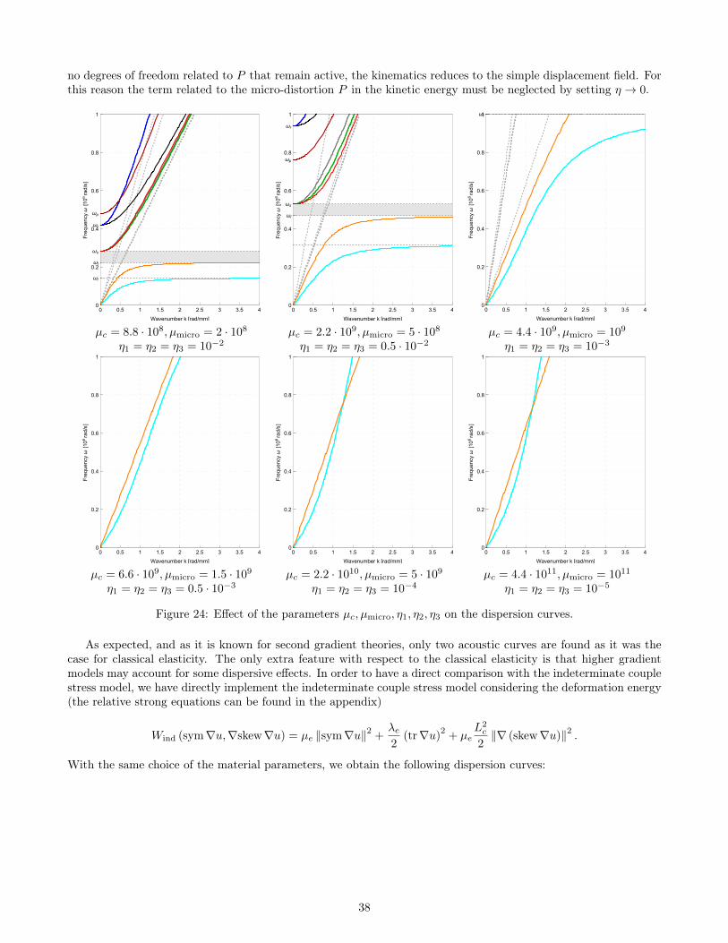
no degrees of freedom related to P that remain active, the kinematics reduces to the simple displacement field. Forthis reason the term related to the micro-distortion P in the kinetic energy must be neglected by setting η → 0.

0 0.5 1 1.5 2 2.5 3 3.5 40

0.2

0.4

0.6

0.8

ωl

ωp

ωr

ωs

ωt

1


Frequency

ω[106rad/s]

0 0.5 1 1.5 2 2.5 3 3.5 40

0.2

0.4

0.6

0.8

ωl

ωp

ωr

ωs

1


Frequency

ω[106rad/s]

0 0.5 1 1.5 2 2.5 3 3.5 40

0.2

0.4

0.6

0.8

ωt1


Frequency

ω[106rad/s]

µc = 8.8 · 108, µmicro = 2 · 108 µc = 2.2 · 109, µmicro = 5 · 108 µc = 4.4 · 109, µmicro = 109

η1 = η2 = η3 = 10−2 η1 = η2 = η3 = 0.5 · 10−2 η1 = η2 = η3 = 10−3

0 0.5 1 1.5 2 2.5 3 3.5 40

0.2

0.4

0.6

0.8

1


Frequency

ω[106rad/s]

0 0.5 1 1.5 2 2.5 3 3.5 40

0.2

0.4

0.6

0.8

1


Frequency

ω[106rad/s]

0 0.5 1 1.5 2 2.5 3 3.5 40

0.2

0.4

0.6

0.8

1


Frequency

ω[106rad/s]

µc = 6.6 · 109, µmicro = 1.5 · 109 µc = 2.2 · 1010, µmicro = 5 · 109 µc = 4.4 · 1011, µmicro = 1011

η1 = η2 = η3 = 0.5 · 10−3 η1 = η2 = η3 = 10−4 η1 = η2 = η3 = 10−5

Figure 24: Effect of the parameters µc, µmicro, η1, η2, η3 on the dispersion curves.

As expected, and as it is known for second gradient theories, only two acoustic curves are found as it was thecase for classical elasticity. The only extra feature with respect to the classical elasticity is that higher gradientmodels may account for some dispersive effects. In order to have a direct comparison with the indeterminate couplestress model, we have directly implement the indeterminate couple stress model considering the deformation energy(the relative strong equations can be found in the appendix)

Wind (sym∇u,∇skew∇u) = µe ‖sym∇u‖2 +λe2

(tr∇u)2

+ µeL2c

2‖∇ (skew∇u)‖2 .

With the same choice of the material parameters, we obtain the following dispersion curves:

38

0 0.5 1 1.5 2 2.5 3 3.5 40

0.2

0.4

0.6

0.8

1


ω[106rad/s]

Figure 25: Dispersion curves indeterminate couple stress model.

ConclusionIn this paper we present for the first time the “weighted” relaxed micromorphic model, by introducing the Cartan-Liedecomposition of the second order tensors P,t and CurlP in the kinetic and elastic energies, respectively. It is foundthat the split of the tensor P,t in the micro-inertia provides a unique feature to the model, namely the possibilityof separately controlling the cut-offs of the optic curves in the dispersion diagram. This is an essential feature inview of the calibration of the relaxed micromorphic parameters on real band-gap metamaterials. The split of thesecond order tensor CurlP presents some effects on the dispersion curves which are less clearly related to possiblephysical situations. In general, we can say that the term dev symCurlP governs, to a large extent, the non-localityin the considered metamaterials since it is able to give rise to a horizontal optic curve. On the other hand, the termskewCurlP is able to grant the onset of (extra) horizontal asymptotes for some optic curves. No specific effect canbe attributed to the term tr (CurlP ).

Another important result of the present paper is that of showing the fundamental role of micro-inertia termswhen dealing with enriched continua. It is shown that both the cases η → 0 and η → ∞ give rise to a Cauchy-type situation in which only 2 straight acoustic branches can be recognized. Nevertheless, the physical meaningassociated to such two cases is completely different. Indeed, setting η = 0 in a model with enriched kinematics canbe considered to be a mistake since one gives a complex and rich behavior to the elastic energy (through a particulardependence on P ), but one does not allow the exploitation of such constitutive behavior due to the absence of theassociated micro-inertia. It is hence not astonishing that, no matter how complex is the constitutive choice for theelastic energy (Mindlin, relaxed micromorphic, Cauchy, second gradient, etc.), the resulting dispersion curves arebasically those of classical elasticity: two straight lines starting from the origin. The problem is simply that we donot give to the model the possibility to express its dynamical behavior since there is no micro-inertia that is ableto trigger micro-vibrations.

On the other hand, the case η → ∞ is phenomenologically different: we introduce the micro-inertia in themodel, but it is so “high” that the microstructure is “frozen” and this results in Cauchy-like materials. We leave toa forthcoming paper the task of studying in greater detail the importance of the role of micro-inertia in enrichedcontinuum mechanics. Finally, some parametric studies on all of the introduced constitutive parameters are per-formed, thus giving a complete panorama of all possible dispersion patterns which are attainable in the relaxedmicromorphic framework.

6 AcknowledgmentsAngela Madeo thanks INSA-Lyon for the funding of the BQR 2016 "Caractérisation mécanique inverse des mé-tamatériaux: modélisation, identification expérimentale des paramètres et évolutions possibles", as well as theCNRS-INSIS for the funding of the PEPS project.

39

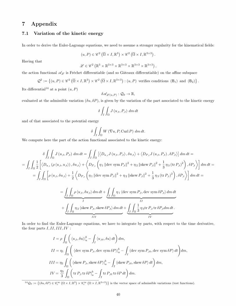
7 Appendix

7.1 Variation of the kinetic energy

In order to derive the Euler-Lagrange equations, we need to assume a stronger regularity for the kinematical fields:

(u, P ) ∈ C 2(Ω× I,R3

)× C 2

(Ω× I,R3×3

).

Having thatL ∈ C 2

(R3 × R3×3 × R3×3 × R3×3 × R3×3

),

the action functional AL is Fréchet differentiable (and so Gâteaux differentiable) on the affine subspace

Q2 :=

(u, P ) ∈ C 2(Ω× I,R3

)× C 2

(Ω× I,R3×3

): (u, P ) verifies conditions (B1) and (B2)

.

Its differential14 at a point (u, P )δAL (u,P ) : Q0 → R,

evaluated at the admissible variation (δu, δP ), is given by the variation of the part associated to the kinetic energy

δ

∫I

∫Ω

J (u,t, P,t) dmdt

and of that associated to the potential energy

δ

∫I

∫Ω

W (∇u, P,CurlP ) dmdt.

We compute here the part of the action functional associated to the kinetic energy:

δ

∫I

∫Ω

J (u,t, P,t) dmdt =

∫I

∫Ω

[⟨Du,tJ (u,t, P,t) , δu,t

⟩+⟨DP,tJ (u,t, P,t) , δP,t

⟩]dmdt =

=

∫I

∫Ω

1

2

[⟨Du,t (ρ 〈u,t, u,t〉) , δu,t

⟩+

⟨DP,t


1

3η 3 (trP,t)

2

), δP,t

⟩]dmdt =

=

∫I

∫Ω

[ρ 〈u,t, δu,t〉+

1

2

⟨DP,t


1

3η 3 (trP,t)

2

), δP,t

⟩]dmdt =

=

∫I

∫Ω

ρ 〈u,t, δu,t〉 dmdt︸︷︷︸I

+

∫I

∫Ω

η 1 〈dev symP,t, dev sym δP,t〉 dmdt︸︷︷︸II

+

∫I

∫Ω

η 2 〈skewP,t, skew δP,t〉 dmdt︸︷︷︸III

+

∫I

∫Ω

1

3η 3trP,t tr δP,tdmdt︸︷︷︸

IV

.

In order to find the Euler-Lagrange equations, we have to integrate by parts, with respect to the time derivative,the four parts I, II, III, IV :

I = ρ

∫Ω

(〈u,t, δu〉|ba −

∫I

〈u,tt, δu〉 dt)dm,

II = η1

∫Ω

(〈dev symP,t, dev sym δP 〉|ba −

∫I

〈dev symP,tt, dev sym δP 〉 dt

)dm,

III = η2

∫Ω

(〈skewP,t, skew δP 〉|ba −

∫I

〈skewP,tt, skew δP 〉 dt)dm,

IV =η3

3

∫Ω

(trP,t tr δP |ba −

∫I

trP,tt tr δP dt)dm.

14Q0 :=

(δu, δP ) ∈ C∞c(Ω× I,R3

)× C∞c

(Ω× I,R3×3

)is the vector space of admissible variations (test functions).

40

Considering that

〈dev symP,tt, dev sym δP 〉 = 〈dev symP,tt, δP 〉 ,〈skewP,tt, skew δP 〉 = 〈skewP,tt, δP 〉 ,

trP,tt tr δP =

⟨tr (P,tt)1,

1

3tr (δP )1

⟩= 〈tr (P,tt)1, δP 〉 , (67)

we find that

I = ρ

∫Ω

(〈u,t, δu〉|ba −

∫I

〈u,tt, δu〉 dt)dm,

II = η1

∫Ω

(〈dev symP,t, δP 〉|ba −

∫I

〈dev symP,tt, δP 〉 dt)dm,

III = η2

∫Ω

(〈skewP,t, δP 〉|ba −

∫I

〈skewP,tt, δP 〉 dt)dm,

IV =η3

3

∫Ω

(〈tr (P,t)1, δP 〉|ba −

∫I

〈tr (P,tt)1, δP 〉 dt)dm.

So considering only the bulk part , we have

δ

∫I

∫Ω

J (u,t, P,t) dmdt = −∫

Ω

∫I

(〈u,tt, δu〉+

⟨η 1 dev symP,tt + η 2 skewP,tt +

1

3η 3 tr (P,tt)1, δP

⟩)dt dm.

7.2 Variation of the part B of the potential energy

Remembering (4), the first variation of the action functional is computed thanks to the following identities:

〈dev symCurlP, δ dev symCurlP 〉 = 〈dev symCurlP,Curl δP 〉R3×3 =

3∑i=1

〈(dev symCurlP )i , (Curl δP )i〉R3

=

3∑i=1

〈(dev symCurlP )i , curl (δP )i〉R3

= −3∑i=1

(div ((dev symCurlP )i × (δP )i) + 〈curl (dev symCurlP )i , (δP )i〉R3

)= −

3∑i=1

div ((dev symCurlP )i × (δP )i) + 〈Curl dev symCurlP, δP 〉R3×3 ,

〈skewCurlP, δ skewCurlP 〉 = 〈skewCurlP,Curl δP 〉 =

3∑i=1

〈(skewCurlP )i , (Curl δP )i〉R3

= −3∑i=1

div ((skewCurlP )i × (δP )i) + 〈Curl skewCurlP, δP 〉R3×3 (68)

1

3tr (CurlP ) δtr (CurlP ) =

⟨1

3tr (CurlP )1,Curl δP

⟩=

3∑i=1

⟨(1

3tr (CurlP )1

)i

, (Curl δP )i

⟩R3

= −3∑i=1

div((

1

3tr (CurlP )1

)i

× (δP )i

)+

⟨Curl

1

3tr (CurlP )1, δP

⟩R3×3

.

7.3 Derivation of PDEs in the new variablesThe following identities will be useful in the following.

41

(Curl dev symCurlP )ij = εjmn (dev symCurlP )in,m = εjmn

(1

2εnpqPiq,p +

1

2εipqPnq,p −

1

3δin (CurlP )kk

),m

=1

2(εjmnεnpqPiq,pm + εjmnεipqPnq,pm)− 1

3εjmiεkpqPkq,pm,

(Curl skewCurlP )ij = εjmn (skewCurlP )in,m = εjmn1

2(εnpqPiq,p − εipqPnq,p),m (69)

=1

2(εjmnεnpqPiq,pm − εjmnεipqPnq,pm) ,(

Curl(

1

3tr (CurlP )1

))ij

= εjmn

(1

3tr (CurlP )1

)in,m

=1

3εjmn ((CurlP )kk δin)

,m

=1

3εjmnδin (εkpqPkq,pm) =

1

3εjmiεkpqPkq,pm.

We set∆ :=

(α1 Curl dev symCurlP + α2 Curl skewCurlP + α3 Curl

(1

3tr (CurlP )1

)). (70)

Equations in u,tt

ρ u,tt = Div [2µe sym (∇u− P ) + λe tr (∇u− P )1+ 2µc skew (∇u− P )] ,

This set of equations can be rewrite as follows:

ρ u,tt = Div [2µe sym (∇u− P ) + λe tr (∇u− P )1+ 2µc skew (∇u− P )]

= Div[2µe dev sym (∇u− P ) +

(2

3µe + λe

)tr (∇u− P )1+ 2µc skew (∇u− P )

]= Div

[2µe dev sym∇u+

(2

3µe + λe

)tr (∇u)1+ 2µc skew (∇u)

](71)

−Div[2µe dev symP +

(2

3µe + λe

)tr (P )1+ 2µc skew (P )

].

Remembering the definitions of u(1,k), P(1k), PD, PS , u[1,k] − P[1k] given in (20),(21),(22), the scalar components of

this vectorial system are therefore

ρ u1,tt = div

2µe

13 (2u1,1 − u2,2 − u3,3)− PD

u(1,2) − P(12)

u(1,3) − P(13)

+

(2

3µe + λe

)∑α uα,α − 3PS

00

+ 2µc

0u[1,2] − P[12]

u[1,3] − P[13]

,

ρ u2,tt = div

2µe

u(1,2) − P(12)13 (2u2,2 − u1,1 − u3,3)− PD2

u(2,3) − P(23)

+

(2

3µe + λe

) 0∑α uα,α − 3PS

0

+ 2µc

−u[1,2] + P[12]

0u[1,3] − P[13]

,

(72)

ρ u3,tt = div

2µe

u(1,3) − P(13)

u(2,3) − P(23)13 (2u1,1 − u2,2 − u3,3)− PD3

+

(2

3µe + λe

) 00∑

α uα,α − 3PS

+ 2µc

−u[1,3] + P[13]

−u[2,3] + P[23]

0

.

Thanks to the hypothesis of dependence only on x1, we have that u2,2, u3,3, u3,2, u2,3 are zero and u(1,2) =12 u2,1, u(1,3) = 1

2 u3,1, u[1,2] = − 12 u2,1, u[1,3] = − 1

2 u3,1. Thus the first equation of (72) becomes

ρ u1,tt =

(2µe

(2

3u1,1 − PD

)+

(2

3µe + λe

)(u1,1 − 3PS

)),1

+

(2µe

(1

2u2,1 − P(12)

)+ 2µc

(−1

2u2,1 − P[12]

)),2︸︷︷︸

=0 (plane wave)

+

(2µe

(1

2u3,1 − P(13)

)+ 2µc

(−1

2u3,1 − P[13]

)),3︸︷︷︸

=0 (plane wave)

= (2µe + λe)u1,11 − 2µe PD,1 − 3

(2

3µe + λe

)PS,1.

42

Dividing by ρ and remembering the definition of cp given in (43) we can rewrite this equation as:

u1,tt = c2p u1,11 −2µeρ

PD,1 −2µe + 3λe

ρPS,1. (73)

Repeating the same calculation for the other two equations, and remembering the definition of cs and ωr given in(43) and (40), we find

uξ,tt = c2s uξ,11 −2µeρ

P(1ξ),1 + ω2r

η2

ρP[1ξ],1, ξ ∈ 2, 3 . (74)

Equations in dev symP,tt

The PDEs system

η 1 dev symP,tt = 2µe dev sym (∇u− P )− 2µmicro dev symP (75)

− µe L2c dev sym


(1

3tr (CurlP )1

)),

has only five independent equations. Setting Eq1 for the system (75) of PDEs, the five independent equations thatwe will take are (Eq1)11 ,(Eq1)12 ,(Eq1)13 ,(Eq1)23 and (Eq1)22 − (Eq1)33 . In order to find the desired PDEs, weneed the following calculations: we have

(sym∆)11 = ∆11 = α1

1

2(ε1mnεnpqP1q,pm + ε1mnε1pqPnq,pm)− 1

3ε1m1︸︷︷︸

0

εkpqPkq,pm

(76)

+ α21

2(ε1mnεnpqP1q,pm − ε1mnε1pqPnq,pm) + α3

1

3ε1m1︸︷︷︸

0

εkpqPkq,pm ,

where ∆ is defined in (70), and remembering that Phk,pq = 0 for every p, q 6= 1 we find

(sym∆)11 = α11

2(ε11nεn1qP1q,11 + ε11nε11qPnq,11) + α2

1

2(ε11nεn1qP1q,11 − ε11nε11qPnq,11) ≡ 0.

For the trace we find

tr∆ =1

2[α1 (εkmnεnpqPkq,pm + εkmnεkpqPnq,pm) + α2 (εkmnεnpqPkq,pm − εkmnεkpqPnq,pm)]

=α1 + α2

2εkmnεnpqPkq,pm +

α1 − α2

2εkmnεkpqPnq,pm

=α1 + α2

2εk1nεn1qPkq,11 +

α1 − α2

2εk1nεk1qPnq,11

=α1 + α2

2(ε213ε312P22,11 + ε312ε213P33,11) +

α1 − α2

2(ε213ε213P33,11 + ε312ε312P22,11)

=α1 + α2

2(−P22,11 − P33,11) +

α1 − α2

2(P33,11 + P22,11)

= −α2 (P22,11 + P33,11) = −α2

(2PS,11 − PD,11

). (77)

Equation 1

We have

(dev sym∆)11 = (sym∆)11 −1

3tr∆ =

α2

3

(2PS,11 − PD,11

).

Thus the first equation is

η 1PD,tt = 2µe

(2

3u1,1 − PD

)− 2µmicroP

D − µeL2c

α2

3

(2PS,11 − PD,11

),

and remembering the definitions of ωs and cm given in (40) and (43) we find

PD,tt =4

3

µeη 1

u1,1 +1

3

α2

η 1µeL

2c P

D,11 −

2

3

α2

η 1µeL

2c P

S,11 − ω2

s PD. (78)

43

Equations 2,3

η 1P(1ξ),tt = 2µe(u(1,ξ) − P(1ξ)

)− 2µmicroP(1ξ) − µeL2

c ∆(1ξ) (79)

= µe uξ,1 − 2 (µe + µmicro)P(1ξ) − µeL2c ∆(1ξ).

We have to calculate the term ∆(1ξ):

(Curl dev symCurlP )(1ξ) =1

4(εξmnεnpqP1q,pm + εξmnε1pqPnq,pm + ε1mnεnpqPξq,pm + ε1mnεξpqPnq,pm)

=1

4(εξ1nεn1qP1q,11 + εξ1nε11qPnq,11 + ε11nεn1qPξq,11 + ε11nεξ1qPnq,11)

=1

4(εξ1nεn1qP1q,11) = −1

4

(P(1ξ),11 + P[1ξ],11

),

(Curl skewCurlP )(1ξ) = −1

4

(P(1ξ),11 + P[1ξ],11

),(

Curl(

1

3tr (CurlP )1

))(1ξ)

=1

2

(1

3εξm1εkpqPkq,pm +

1

3ε1mξεkpqPkq,pm

)=

1

2

(1

3εξ11εk1qPkq,11 +

1

3ε11ξεk1qPkq,11

)= 0.

So we have

η 1P(1ξ),tt = 2µe(u(1,ξ) − P(1ξ)

)− 2µmicroP(1ξ) + µeL

2c

α1 + α2

4

(P(1ξ),11 + P[1ξ],11

)(80)

P(1ξ),tt =µeη 1

u(1,ξ) + µeL2c

α1 + α2

4P(1ξ),11 + µeL

2c

α1 + α2

4P[1ξ],11 − ω2

sP(1ξ).

Equation 4

η 1P(23),tt = 2µe(u(2,3) − P(23)

)− 2µmicroP(23) − µeL2

c ∆(23) (81)

= −2 (µe + µmicro)P(23) − µeL2c ∆(23).

We have to calculate the term ∆(23):

(Curl dev symCurlP )(23) =1

4(ε3mnεnpqP2q,pm + ε3mnε2pqPnq,pm + ε2mnεnpqP3q,pm + ε2mnε3pqPnq,pm)

=1

4(ε31nεn1qP2q,11 + ε31nε21qPnq,11 + ε21nεn1qP3q,11 + ε21nε31qPnq,11)

=1

4(ε312ε213P23,11 + ε312ε213P23,11 + ε213ε312P32,11 + ε213ε312P32,11)

= −1

2(P23,11 + P32,11) = −P(23),11,

(Curl skewCurlP )(23) =1

4(ε312ε213P23,11 − ε312ε213P23,11 + ε213ε312P32,11 − ε213ε312P32,11) = 0,(

Curl(

1

3tr (CurlP )1

))(23)

=1

2

(1

3ε3m2εkpqPkq,pm +

1

3ε2m3εkpqPkq,pm

)=

1

2

(1

3ε312εk1qPkq,11 +

1

3ε213εk1qPkq,11

)= 0.

Thus we have

η 1P(23),tt = −2 (µe + µmicro)P(23) + µeL2c α1P(23),11

P(23),tt = −ω2s P(23) +

(cdm)2P(23),11 . (82)

Equation 5

We have to determine (Eq1)22 − (Eq1)33 . So

η 1PD2,tt = 2µe

(u2,2 −

1

3uk,k − PD2

)− 2µmicroP

D2 − µeL2

c

(∆22 −

1

3tr (∆)

)=

2

3µeu1,1 − (2µe + 2µmicro)PD2 − µeL2

c

(∆22 −

1

3tr (∆)

),

44

and

η 1PD3,tt = 2µe

(u3,3 −

1

3uk,k − PD3

)− 2µmicroP

D3 − µeL2

c

(∆33 −

1

3tr (∆)

)=

2

3µeu1,1 − (2µe + 2µmicro)PD3 − µeL2

c

(∆33 −

1

3tr (∆)

).

Thus, for (Eq1)22 − (Eq1)33 we find

η 1PV,tt = − (2µe + 2µmicro)PV − µeL2

c (∆22 −∆33) (83)

and having that

(Curl dev symCurlP )22 =1

2(ε2mnεnpqP2q,pm + ε2mnε2pqPnq,pm)− 1

3ε2m2εkpqPkq,pm

=1

2(ε21nεn1qP2q,11 + ε21nε21qPnq,11)

=1

2(ε213ε312P22,11 + ε213ε213P33,11)

=1

2(−P22,11 + P33,11) = −1

2PV,11 (84)

= − (Curl dev symCurlP )33 ,

(Curl skewCurlP )22 =1

2(ε2mnεnpqP2q,pm − ε2mnε2pqPnq,pm)

=1

2(ε213ε312P22,11 − ε213ε213P33,11)

= −1

2(P22,11 + P33,11) = (Curl skewCurlP )33 ,(

Curl(

1

3tr (CurlP )1

))22

= 0 =

(Curl

(1

3tr (CurlP )1

))33

.

Thus we have

η 1PV,tt = − (2µe + 2µmicro)PV + µeL

2c α1 P

V,11

PV,tt = −ω2sP

V +(cdm)2PV,11. (85)

Equations in skewP,tt

The PDEs system

η 2 skewP,tt = 2µc skew (∇u− P )

− µe L2c skew


(1

3tr (CurlP )1

)),

has only three independent equations.

Equations 1,2

η 2P[1ξ],tt = 2µc(u[1,ξ] − P[1ξ]

)− µe L2

c ∆[1ξ] (86)

= 2µc(−uξ,1 − P[1ξ]

)− µe L2

c ∆[1ξ], ξ ∈ 2, 3

45

we have to calculate the term ∆[1ξ]:

(Curl dev symCurlP )[1ξ] =1

4(εξmnεnpqP1q,pm + εξmnε1pqPnq,pm − ε1mnεnpqPξq,pm − ε1mnεξpqPnq,pm)

=1

4(εξ1nεn1qP1q,11 + εξ1nε11qPnq,11 − ε11nεn1qPξq,11 − ε11nεξ1qPnq,11)

=1

4(εξ1nεn1qP1q,11) = −1

4

(P(1ξ),11 + P[1ξ],11

),

(Curl skewCurlP )[1ξ] = −1

4

(P(1ξ),11 + P[1ξ],11

),(

Curl(

1

3tr (CurlP )1

))[1ξ]

=1

2

(1

3εξm1εkpqPkq,pm −

1

3ε1mξεkpqPkq,pm

)=

1

2

(1

3εξ11εk1qPkq,11 −

1

3ε11ξεk1qPkq,11

)= 0.

So we have

η 2P[1ξ],tt = 2µc(u[1,ξ] − P[1ξ]

)− µe L2

c ∆[1ξ]

P[1ξ],tt = −1

2ω2r uξ,1 − ω2

r P[1ξ] + µe L2c

α1 + α2

4 η2

(P(1ξ),11 + P[1ξ],11

).

Equation 3

η 2P[23],tt = 2µc(u[2,3] − P[23]

)− µeL2

c ∆[23] = −2µc P[23] − µeL2c ∆[23]. (87)

We have to calculate the term ∆[23]:

(Curl dev symCurlP )[23] =1

4(ε3mnεnpqP2q,pm + ε3mnε2pqPnq,pm − ε2mnεnpqP3q,pm − ε2mnε3pqPnq,pm)

− 1

3ε3m2εkpqPkq,pm

=1

4(ε31nεn1qP2q,11 + ε31nε21qPnq,11 − ε21nεn1qP3q,11 − ε21nε31qPnq,11)

− 1

3ε312εk1qPkq,11

=1

4(ε312ε213P23,11 + ε312ε213P23,11 − ε213ε312P32,11 − ε213ε312P32,11)

− 1

3(ε213P23,11 + ε312P32,11)

=1

2(−P23,11 + P32,11)− 1

3(−P23,11 + P32,11) = −1

3P[23],11,

(Curl skewCurlP )[23] =1

4(ε312ε213P23,11 − ε312ε213P23,11 + ε213ε312P32,11 − ε213ε312P32,11) = 0,(

Curl(

1

3tr (CurlP )1

))[23]

=1

2

(1

3ε3m2εkpqPkq,pm −

1

3ε2m3εkpqPkq,pm

)=

1

2

(1

3ε312εk1qPkq,11 −

1

3ε213εk1qPkq,11

)=

1

6(ε213P23,11 + ε312P32,11 + ε213P23,11 + ε312P32,11) = −2

3P[23],11.

So we have

η 2P[23],tt = −2µc P[23] + µeL2c

(α1 + 2α3

3

)P[23],11

P[23],tt = −ω2r P[23] +

(cvdm

)2P[23],11.

Equations in the spherical part of P,tt

1

3η 3 tr (P,tt) =

(2

3µe + λe

)tr (∇u− P )−

(2

3µmicro + λmicro

)tr (P )

− µe L2c

1

3tr(α1 Curl dev symCurlP + α2 Curl skewCurlP +

α3


).

46

Considering the expression (77) for the tr (∆), we have

PS,tt =2µe + 3λe

3 η3u1,1 − ω2

p PS +

µe L2c α2

η3

(2

3PS,11 −

1

3PD,11

).

7.4 Determination of slopes of the acoustic branchesWe want to evaluate the first and second derivative in 0 of the expressions

detEα (k, ωaco;α (k)) =

3∑p,q=1

ψ(α)pq (m) k2pω2q

aco;α (k) +

3∑p=1

ϕ(α)p (m) k2p +

3∑q=1

ζ(α)q (m) ω2q

aco;α (k) + σ(α) (m) ,

with α ∈ 1, 2. In order to work with a more readable notation, in what follows we suppress the dependence bym and k of the relative functions. The derivative of ωaco;α with respect to k is denoted by ω′aco;α . We have

d

dkdetEα (k, ωaco;α) =

3∑p,q=1

ψ(α)pq

(2p k2p−1ω2q

aco;α + 2q k2pω2q−1aco;α ω

′aco;α

)+

3∑p=1

2pϕ(α)p k2p−1 +

3∑q=1

2q ζ(α)q ω2q−1

aco;α ω′aco;α,

and so, remembering that ωaco;α (0) = 0, this condition does not give any information on the value of ω′aco;α (0).For this reason, we continue with the second derivative. We compute separately the derivative of the four terms ofthe first derivative of detEα (k, ωaco;α (k)) obtaining:

d

dk

3∑p,q=1

2pψ(α)pq k

2p−1ω2qaco;α =

3∑p,q=1

2pψ(α)pq

((2p− 1) k2p−2ω2q

aco;α + 2q k2p−1ω2q−1aco;αω

′aco;α

),

d

dk

3∑p,q=1

2q ψ(α)pq k

2pω2q−1aco;α ω

′aco;α =

3∑p,q=1

2q ψ(α)pq

(2p k2p−1ω2q−1

aco;α ω′aco;α + k2p

((2q − 1) ω2q−2

aco;α

(ω′aco;α

)2+ ω2q−1

aco;α ω′′aco;α

)),

d

dk

3∑p=1

2pϕ(α)p k2p−1 =

3∑p=2

2p (2p− 1)ϕ(α)p k2p−2 + 2ϕ

(α)1 ,

d

dk

3∑q=1

2q ζ(α)q ω2q−1

aco;α ω′aco;α =

3∑p=2

2p ζ(α)q

((2q − 1) ω2q−2

aco;α

(ω′aco;α

)2+ ω2q−1

aco;α ω′′aco;α

)+ 2 ζ

(α)1

((ω′aco;α

)2+ ωaco;α ω

′′aco;α

).

Thus

0 =d2

dk2detEα (k, ωaco;α (k))|k=0 = 2 ζ

(α)1

(ω′aco;α (0)

)2+ 2ϕ

(α)1 . (88)

Solving the equations (88) we find

2 ζ(α)2

(ω′aco;α (0)

)2+ 2ϕ

(α)1 = 0 ⇐⇒

(ω′aco;α (0)

)2=−ϕ(α)

1

ζ(α)1

and so, considering only the positive roots,

ω′aco;1 (0) =

√√√√−ϕ(1)1

ζ(1)1

, and ω′aco;2 (0) =

√√√√−ϕ(2)1

ζ(2)1

.

7.5 Derivation of strong equations for the Cosserat model and indeterminate couplestress model

In this appendix we give the strong field equations for the Cosserat model and the indeterminate couple stressmodel.

47

Cosserat model

The potential weighted energy for the Cosserat model is the following

Wcos = µe ‖sym∇u‖2 + µc ‖skew (∇u− P )‖2 +λe2

(tr∇u)2 (89)

+ µeL2c

2

(α1 ‖dev symCurl skewP‖2 + α2 ‖skewCurl skewP‖2 +

1

3α3 (tr Curl skewP )

2

).

The first variation is computed exactly in the same way as in (11), giving the following system of PDEs:

ρ u,tt = Div [2µe sym∇u+ λe tr (∇u)1 + 2µc skew (∇u− P )] , (90)

η2 skewP,tt = −µe L2c skewCurl

[α1dev symCurl skewP + α2 skewCurl skewP +

α3

3tr (Curl skewP )1

]+ 2µc skew (∇u− P ) .

The system of PDEs (90) is not really suitable for the numerical implementation. Working only with the skewsymmetric part of the micro-distortion tensor P , it is more convenient to see skewP like a vector thanks to theidentification of the Lie algebra so (3) with R3 by means of the axl-operator. In this way we can work only withthe six independent equations of the system (90). We remember that for

A =

0 −a3 a2

a3 0 −a1

−a2 a1 0

∈ so (3)

the axl : so (3)→ R3 operator is defined as follows:

axlA := (a1, a2, a3) , (axlA)k = −1

2εijkAij .

Thanks to the identities [37]

−CurlA = (∇axlA)T − tr

[(∇axlA)

T]1,

∇axlA = − (CurlA)T

+1

2tr[(CurlA)

T]1,

verified for every A ∈ so (3), the system of PDEs (90) can be rewritten in a completely equivalent form as

ρ u,tt = Div [2µe sym∇u+ λe tr (∇u)1+ 2µc skew (∇u− P )] ,

η2 (axl skewP ),tt = µe L2c Div

[α1

2dev sym∇ (axl skewP ) +

α2

2skew∇ (axl skewP ) +

2α3

3tr (∇ (axl skewP ))1

]+ 2µc axl skew (∇u− P ) .

Indeterminate couple stress model

The potential weighted energy for the indeterminate couple stress model is the following [14]

Wind 1 (sym∇u,Curl sym∇u) = µe ‖sym∇u‖2 +λe2

(tr∇u)2 (91)

+ µeL2c

2

(α1 ‖dev symCurl sym∇u‖2 + α2 ‖skewCurl sym∇u‖2

).

The first variation of this energy density gives the following system of PDEs:

ρ u,tt = Div [2µe sym∇u+ λe tr (∇u)1]

+ Div[µe L

2c symCurl (2α1 dev symCurl sym∇u+ 2α2 skewCurl sym∇u)

].

The problem can be completely reformulated in terms of the gradient of the skew symmetric part of ∇u. Indeed,thanks to the equivalence

∇ (axl skew∇u) = (Curl sym∇u)T,

48

the following energy density

Wind 2 (sym∇u,∇ (axl skew∇u)) = µe ‖sym∇u‖2 +λe2

(tr∇u)2 (92)

+ µeL2c

2

(α1 ‖dev sym∇ (axl skew∇u)‖2 + α2 ‖skew∇ (axl skew∇u)‖2

).

is completely equivalent to (91). The associated system of Euler- Lagrange equations is

ρ u,tt = Div [2µe sym∇u+ λe tr (∇u)1]

−Div[µe L

2c anti Div (α1 dev sym∇ (axl skew∇u) + α2 skew∇ (axl skew∇u))

],

where anti is the inverse operator of axl defined as follows

anti : R3 → so (3) , (anti (u))ij = −εijkuk.

References[1] Gabriele Barbagallo, Marco Valerio d’Agostino, Rafael Abreu, Ionel-Dumitrel Ghiba, Angela Madeo, and Patrizio Neff. Transparent

anisotropy for the relaxed micromorphic model: macroscopic consistency conditions and long wave length asymptotics. arXivpreprint arXiv:1601.03667, to appear in Int. J. Solids Struct., 2016.

[2] VL Berdichevskii and LI Sedov. Dynamic theory of continuously distributed dislocations. its relation to plasticity theory:vol. 31,no. 6, 1967, pp. 981–1000. Journal of Applied Mathematics and Mechanics, 31(6):989–1006, 1967.

[3] Mircea Birsan and Patrizio Neff. On the dislocation density tensor in the Cosserat theory of elastic shells. arXiv preprintarXiv:1602.03421, 2016.

[4] William D. Claus and Ahmed Cemal Eringen. Three dislocation concepts and micromorphic mechanics. Developments in Mechanics,6:349–358, 1969.

[5] William D. Claus and Ahmed Cemal Eringen. Dislocation dispersion of elastic waves. International Journal of Engineering Science,9(7):605–610, 1971.

[6] NM Cordero, Anais Gaubert, Samuel Forest, Esteban P Busso, F Gallerneau, and S Kruch. Size effects in generalised continuumcrystal plasticity for two-phase laminates. Journal of the Mechanics and Physics of Solids, 58(11):1963–1994, 2010.

[7] François Ebobisse, Klaus Hackl, and Patrizio Neff. A canonical rate-independent model of geometrically linear isotropic gradientplasticity with isotropic hardening and plastic spin accounting for the burgers vector. arXiv preprint arXiv:1603.00271, 2016.

[8] François Ebobisse and Patrizio Neff. Existence and uniqueness for rate-independent infinitesimal gradient plasticity with isotropichardening and plastic spin. Mathematics and Mechanics of Solids, 15(6):691–703, 2010.

[9] François Ebobisse, Patrizio Neff, and Daya Reddy. Existence results in dislocation based rate-independent isotropic gradientplasticity with kinematical hardening and plastic spin: The case with symmetric local backstress. arXiv preprint arXiv:1504.01973,2015.

[10] Ahmed Cemal Eringen. Microcontinuum field theories: I. Foundations and Solids. Springer Science & Business Media, 2012.

[11] Ahmed Cemal Eringen and William D. Claus. A micromorphic approach to dislocation theory and its relation to several existingtheories. Technical report, DTIC Document, 1969.

[12] Samuel Forest. Micromorphic approach for gradient elasticity, viscoplasticity, and damage. Journal of Engineering Mechanics,135(3):117–131, 2009.

[13] Samuel Forest. Nonlinear regularization operators as derived from the micromorphic approach to gradient elasticity, viscoplasticityand damage. In Proc. R. Soc. A, volume 472. The Royal Society, 2016.

[14] Ionel-Dumitrel Ghiba, Patrizio Neff, Angela Madeo, and Ingo Münch. A variant of the linear isotropic indeterminate couple-stressmodel with symmetric local force-stress, symmetric nonlocal force-stress, symmetric couple-stresses and orthogonal boundaryconditions. Mathematics and Mechanics of Solids, page 1081286515625535, 2016.

[15] Ionel-Dumitrel Ghiba, Patrizio Neff, Angela Madeo, Luca Placidi, and Giuseppe Rosi. The relaxed linear micromorphic continuum:existence, uniqueness and continuous dependence in dynamics. Mathematics and Mechanics of Solids, 20(10):1171–1197, 2015.

[16] Elena F. Grekova. Linear reduced Cosserat medium with spherical tensor of inertia, where rotations are not observed in experiment.Mechanics of Solids, 47(5):538–543, 2012.

[17] Ekkehart Kröner. Discussion on papers by A.C. Eringen and W.D. Claus, Jr, and N. Fox. Fundamental Aspects of DislocationTheory, 1:1054–1059.

[18] MA Kulesh, Elena F. Grekova, and IN Shardakov. The problem of surface wave propagation in a reduced Cosserat medium.Acoustical Physics, 55(2):218–226, 2009.

[19] Angela Madeo, Gabriele Barbagallo, Marco Valerio D’Agostino, Rafael Abreu, Ionel-Dumitrel Ghiba, and Patrizio Neff. Real wavepropagation in the isotropic relaxed micromorphic model. accepted Proc. R. Soc. A, 2016.

49

[20] Angela Madeo, Gabriele Barbagallo, Marco Valerio d’Agostino, Luca Placidi, and Patrizio Neff. First evidence of non-locality inreal band-gap metamaterials: determining parameters in the relaxed micromorphic model. In Proc. R. Soc. A, volume 472, page20160169. The Royal Society, 2016.

[21] Angela Madeo, Patrizio Neff, Elias C Aifantis, Gabriele Barbagallo, and Marco Valerio d’Agostino. On the role of micro-inertia inenriched continuum mechanics. arXiv preprint arXiv:1607.07385, 2016.

[22] Angela Madeo, Patrizio Neff, Gabriele Barbagallo, Marco Valerio d’Agostino, and Ionel-Dumitrel Ghiba. A review on wavepropagation modeling in band-gap metamaterials via enriched continuum models. arXiv preprint arXiv:1609.01073, 2016.

[23] Angela Madeo, Patrizio Neff, Marco Valerio d’Agostino, and Gabriele Barbagallo. Complete band gaps including non-local effectsoccur only in the relaxed micromorphic model. arXiv preprint arXiv:1602.04315, 2016.

[24] Angela Madeo, Patrizio Neff, I-D Ghiba, Luca Placidi, and Giuseppe Rosi. Band gaps in the relaxed linear micromorphic continuum.Zeitschrift für Angewandte Mathematik und Mechanik, 95(9):880–887, 2015.

[25] Angela Madeo, Patrizio Neff, Ionel-Dumitrel Ghiba, Luca Placidi, and Giuseppe Rosi. Wave propagation in relaxed micromorphiccontinua: modeling metamaterials with frequency band-gaps. Continuum Mechanics and Thermodynamics, 27(4-5):551–570, 2015.

[26] Angela Madeo, Patrizio Neff, Ionel-Dumitrel Ghiba, and Giuseppe Rosi. Reflection and transmission of elastic waves in non-localband-gap metamaterials: A comprehensive study via the relaxed micromorphic model. Journal of the Mechanics and Physics ofSolids, 95:441 – 479, 2016.

[27] Raymond David Mindlin. Microstructure in linear elasticity. Technical report, Office of Naval Research, 1963.

[28] Raymond David Mindlin. Micro-structure in linear elasticity. Archive for Rational Mechanics and Analysis, 16(1):51–78, 1964.

[29] Ingo Münch and Patrizio Neff. A nonlinear micropolar continuum theory for initial plasticity. Advances and Trends in StructuralEngineering, Mechanics and Computation, pages 269–272, 2010.

[30] Patrizio Neff. On material constants for micromorphic continua. Trends in Applications of Mathematics to Mechanics, STAMMProceedings, Seeheim, pages 337–348, 2004.

[31] Patrizio Neff. Existence of minimizers for a finite-strain micromorphic elastic solid. Proceedings of the Royal Society of Edinburgh:Section A Mathematics, 136(05):997–1012, 2006.

[32] Patrizio Neff. Existence of minimizers in nonlinear elastostatics of micromorphic solids. In Encyclopedia of Thermal Stresses, pages1475–1485. Springer, 2014.

[33] Patrizio Neff, Krzysztof Chełmiński, and Hans-Dieter Alber. Notes on strain gradient plasticity: finite strain covariant modellingand global existence in the infinitesimal rate-independent case. Mathematical Models and Methods in Applied Sciences, 19(02):307–346, 2009.

[34] Patrizio Neff and Samuel Forest. A geometrically exact micromorphic model for elastic metallic foams accounting for affinemicrostructure. modelling, existence of minimizers, identification of moduli and computational results. Journal of Elasticity,87(2-3):239–276, 2007.

[35] Patrizio Neff, Ionel-Dumitrel Ghiba, Markus Lazar, and Angela Madeo. The relaxed linear micromorphic continuum: well-posedness of the static problem and relations to the gauge theory of dislocations. The Quarterly Journal of Mechanics and AppliedMathematics, pages 53–84, 2015.

[36] Patrizio Neff, Ionel-Dumitrel Ghiba, Angela Madeo, Luca Placidi, and Giuseppe Rosi. A unifying perspective: the relaxed linearmicromorphic continuum. Continuum Mechanics and Thermodynamics, 26(5):639–681, 2014.

[37] Patrizio Neff and Ingo Münch. Curl bounds grad on so (3). ESAIM: Control, Optimisation and Calculus of Variations, 14(1):148–159, 2008.

[38] Sergiy Nesenenko and Patrizio Neff. Well-posedness for dislocation based gradient viscoplasticity i: Subdifferential case. SIAMJournal on Mathematical Analysis, 44(3):1694–1712, 2012.

[39] Kim Pham, Varvara G. Kouznetsova, and Marc G. D. Geers. Transient computational homogenization for heterogeneous materialsunder dynamic excitation. Journal of the Mechanics and Physics of Solids, 61(11):2125–2146, 2013.

[40] Valentin L. Popov. Dynamics of plastic rotations in a medium with dislocations and disclinations. Technical Physics Letters,20:576–577, 1994.

[41] Ashwin Sridhar, Varvara G. Kouznetsova, and Marc G.D. Geers. Homogenization of locally resonant acoustic metamaterialstowards an emergent enriched continuum. Computational Mechanics, 57(3):423–435, 2016.

[42] Bob Svendsen, Patrizio Neff, and Andreas Menzel. On constitutive and configurational aspects of models for gradient continuawith microstructure. Zeitschrift für Angewandte Mathematik und Mechanik, 89(8):687–697, 2009.

50

Documents

micromorphic model - arxiv.org