Embed Size (px)
Citation preview
MICROGRIDS OVERVIEW AND
RESEARCH
Claudio Cañizares D e p a r t m e n t o f E l e c t r i c a l & C o m p u t e r E n g i n e e r i n g P o w e r & E n e r g y S y s t e m s ( w w w . p o w e r . u w a t e r l o o . c a )
W I S E ( w w w . w i s e . u w a t e r l o o . c a )
W i t h c o n t e n t a n d s l i d e s f r o m P h D s t u d e n t s D a n i e l O l i v a r e s , M a r i a n o A r r i a g a a n d E h s a n N a s r .
OUTLINE
• Definition and motivations
• Distributed generation (DG): Definition
Technologies
• Optimal planning: Sizing and site selection
• Microgrid control: Voltage and frequency control
Energy management problem
• Stability
2
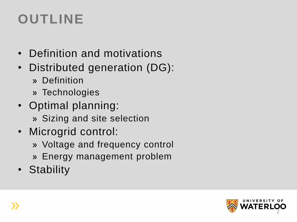
MICROGRID DEFINITION
• There is no “standard” definition, but there is general agreement on what a microgrid is:
A “small” grid from some kW to a few MW.
A “local” grid serving a well-identified, “contained” region.
Operates at distribution system voltage levels, i.e., medium voltage (a few kV).
Contains “various” DG units and possibly some energy storage.
Has enough capacity to supply all or at least most of the loads of the local grid.
Grid connected: has one well-identifiable point of connection to the transmission system or “rest” of the distribution grid (Point of Common Coupling or PCC).
Isolated (islanded): operates independently of the “large” grid.
3
MICROGRID DEFINITION
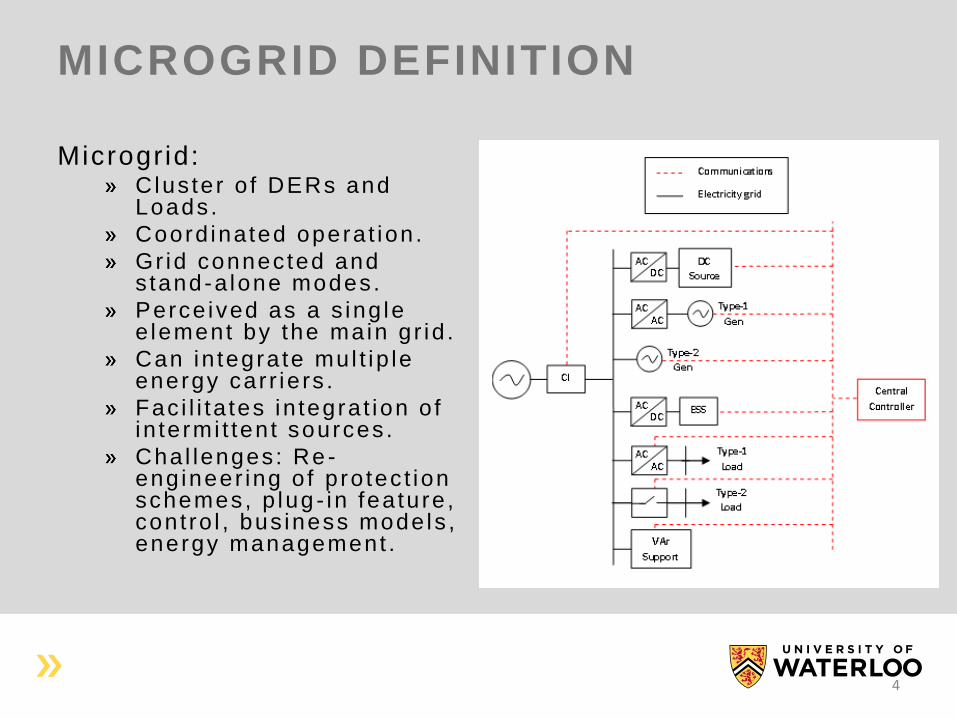
Microgrid: Clus ter o f DERs and Loads .
Coord inated opera t ion .
Gr id connected and s tand-a lone modes.
Perce ived as a s ing le e lement by the main gr id .
Can in tegra te mul t ip le energy car r ie rs .
Fac i l i ta tes in tegra t ion o f in te rmi t ten t sources .
Cha l lenges: Re -eng ineer ing o f p ro tec t ion schemes, p lug - in fea ture , cont ro l , bus iness mode ls , energy management .
4
MICROGRID MOTIVATIONS
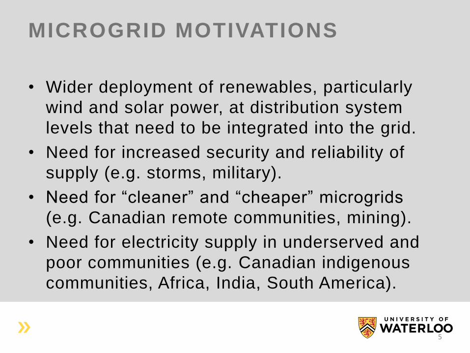
• Wider deployment of renewables, particularly
wind and solar power, at distribution system
levels that need to be integrated into the grid.
• Need for increased security and reliability of
supply (e.g. storms, military).
• Need for “cleaner” and “cheaper” microgrids
(e.g. Canadian remote communities, mining).
• Need for electricity supply in underserved and
poor communities (e.g. Canadian indigenous
communities, Africa, India, South America).
5
DG DEFINITION
• A generation plant connected to the grid at distribution level voltage or on the customer’s side of the meter.
• Integral part of Distributed Energy Resources (DERs).
• No generally accepted definition regarding DG capacity:
DoE: less than a kW to tens of MW.
IEEE: less than 10 MW.
CIGRE: less than 100 MW.
EPRI: a few kW to 50 MW.
6
DG TECHNOLOGIES: RENEWABLE
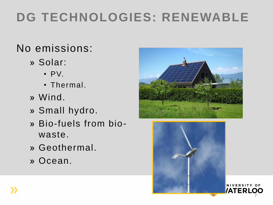
No emissions:
Solar:
• PV.
• Thermal.
Wind.
Small hydro.
Bio-fuels from bio-
waste.
Geothermal.
Ocean.
7
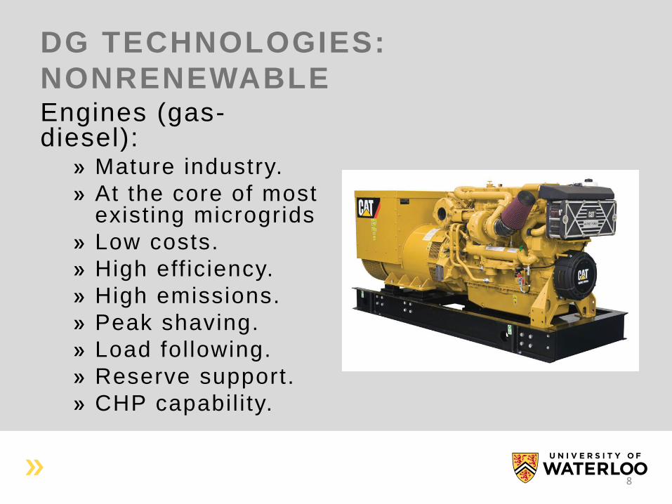
DG TECHNOLOGIES:
NONRENEWABLE Engines (gas-diesel):
Mature industry.
At the core of most exist ing microgrids
Low costs.
High eff iciency.
High emissions.
Peak shaving.
Load following.
Reserve support.
CHP capabil i ty.
8
DG TECHNOLOGIES:
NONRENEWABLE
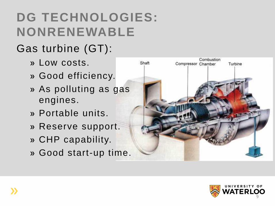
Gas turbine (GT):
Low costs.
Good eff iciency.
As polluting as gas
engines.
Portable units.
Reserve support.
CHP capabil i ty.
Good start-up t ime.
9
DG TECHNOLOGIES:
NONRENEWABLE
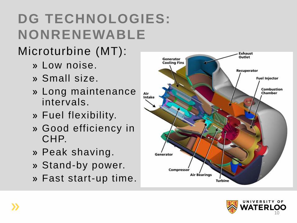
Microturbine (MT): Low noise.
Small size.
Long maintenance intervals.
Fuel f lexibil i ty.
Good eff iciency in CHP.
Peak shaving.
Stand-by power.
Fast start-up t ime.
10
DG TECHNOLOGIES:
RENEWABLE/NONRENEWABLE Fuel cell (FC):
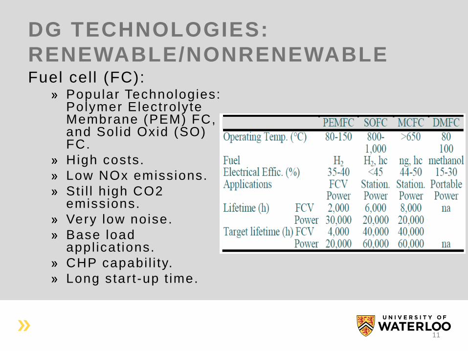
Popular Technologies: Polymer Electrolyte Membrane (PEM) FC, and Sol id Oxid (SO) FC.
High costs.
Low NOx emissions.
Sti l l h igh CO2 emissions.
Very low noise.
Base load appl icat ions.
CHP capabi l i ty.
Long star t -up t ime.
11
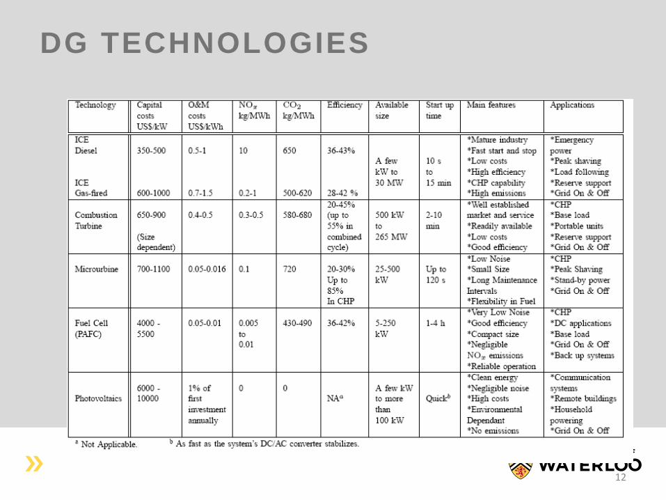
DG TECHNOLOGIES
12
OPTIMAL PLANNING
• Feasibility of installing RE capacity:
Decide most appropriate location(s). • Start with the location(s) with high wind/solar energy
resources (high capacity factors).
• Move then to sites with “less” RE resources.
Optimize for overall project and O&M costs.
Constraints: • Sites with capacity factor above certain level.
• Maximum allowed RE penetration level.
13
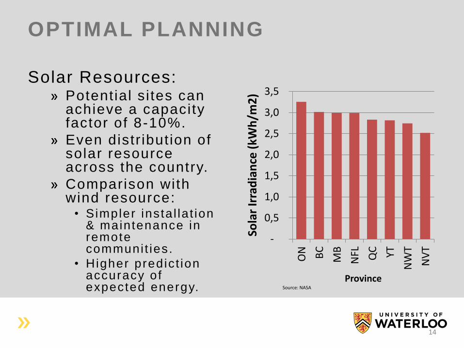
OPTIMAL PLANNING
Solar Resources: Potential s i tes can achieve a capacity factor of 8-10%.
Even distr ibut ion of solar resource across the country.
Comparison with wind resource:
• Simpler insta l la t ion & maintenance in remote communi t ies.
• Higher predic t ion accuracy of expected energy. Source: NASA
-
0,5
1,0
1,5
2,0
2,5
3,0
3,5
ON BC
MB
NFL QC YT
NW
T
NV
T
Sola
r Ir
rad
ian
ce (
kWh
/m2
)
Province
14
OPTIMAL PLANNING
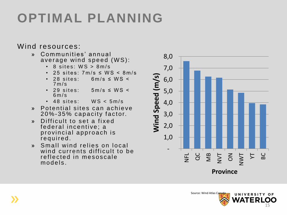
Wind resources: Commun i t i es ’ annua l ave rage w ind speed (W S) :
• 8 s i t e s : W S > 8 m / s
• 2 5 s i t e s : 7 m / s ≤ W S < 8 m / s
• 2 8 s i t e s : 6 m / s ≤ W S < 7 m / s
• 2 9 s i t e s : 5 m / s ≤ W S < 6 m / s
• 4 8 s i t e s : W S < 5 m / s
Po ten t i a l s i t es can ach ieve 2 0 %-35% capac i t y f ac to r.
D i f f i cu l t t o se t a f i xed f ede ra l i n cen t i ve ; a p rov i nc i a l app roach i s r equ i r ed .
Sma l l w ind r e l i e s on l oca l w ind cu r ren ts d i f f i cu l t t o be r e f l ec ted i n mesosca le mode l s .
-
1,0
2,0
3,0
4,0
5,0
6,0
7,0
8,0
NFL QC
MB
NV
T
ON
NW
T YT BC
Win
d S
pe
ed
(m
/s)
Province
Source: Wind Atlas Canada
15
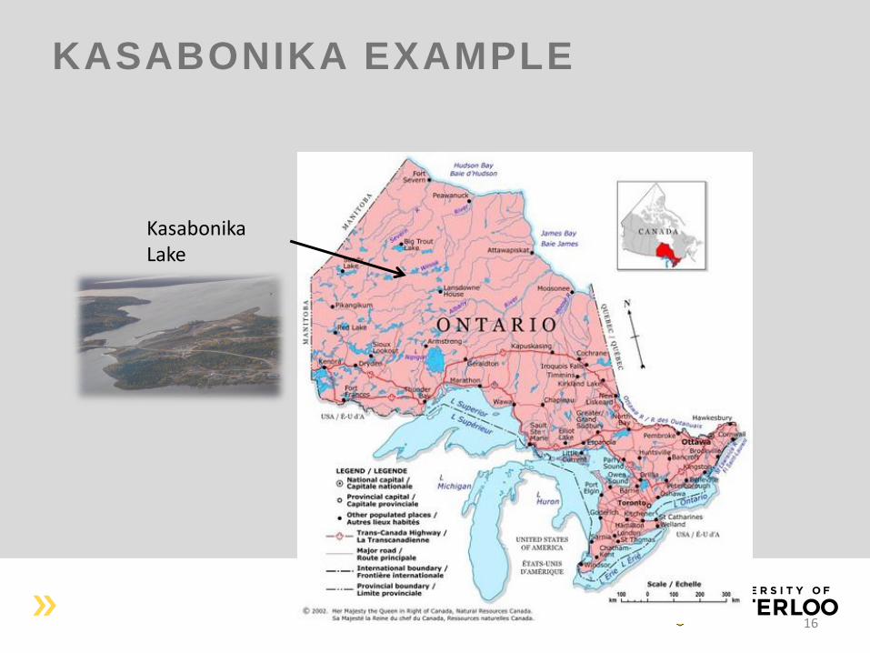
KASABONIKA EXAMPLE
Kasabonika Lake
16
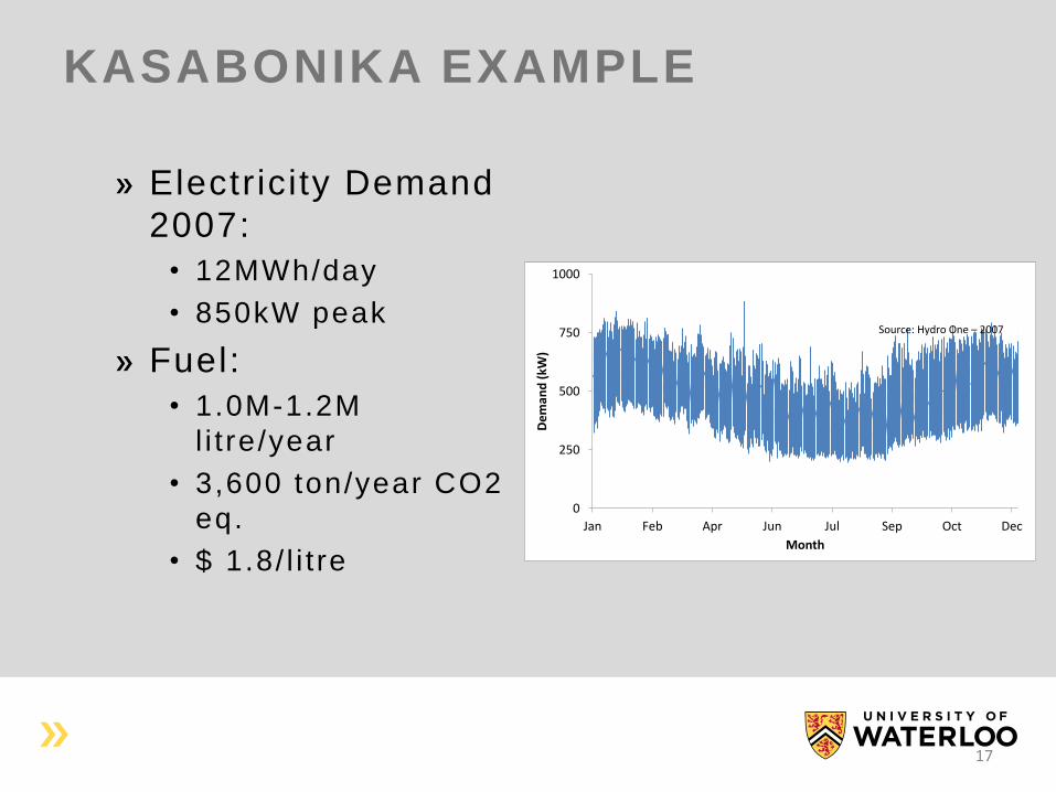
KASABONIKA EXAMPLE
Electricity Demand
2007:
• 12MWh/day
• 850kW peak
Fuel:
• 1.0M-1.2M
l i t re/year
• 3,600 ton/year CO2
eq.
• $ 1.8/ l i t re
0
250
500
750
1000
Jan Feb Apr Jun Jul Sep Oct DecD
em
and
(kW
)Month
Source: Hydro One – 2007
17
KASABONIKA EXAMPLE
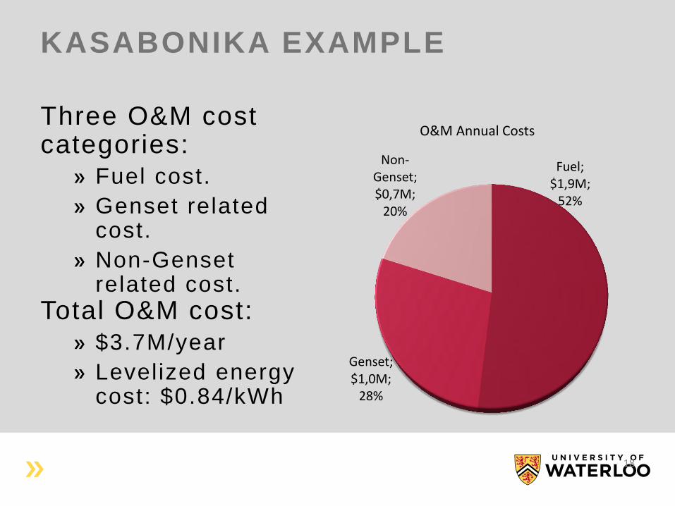
Three O&M cost categories:
Fuel cost.
Genset related cost.
Non-Genset related cost.
Total O&M cost: $3.7M/year
Levelized energy cost: $0.84/kWh
18
Fuel; $1,9M;
52%
Genset; $1,0M;
28%
Non-Genset; $0,7M;
20%
O&M Annual Costs
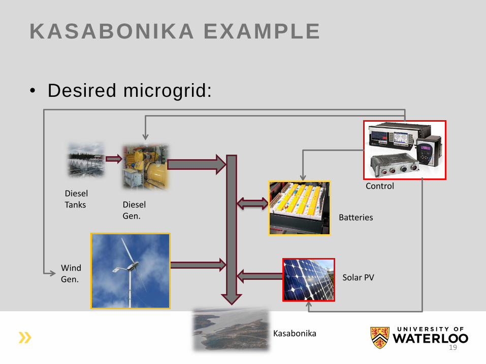
KASABONIKA EXAMPLE
• Desired microgrid:
Diesel Gen.
Diesel Tanks
Wind Gen.
Kasabonika
Solar PV
Batteries
Control
19
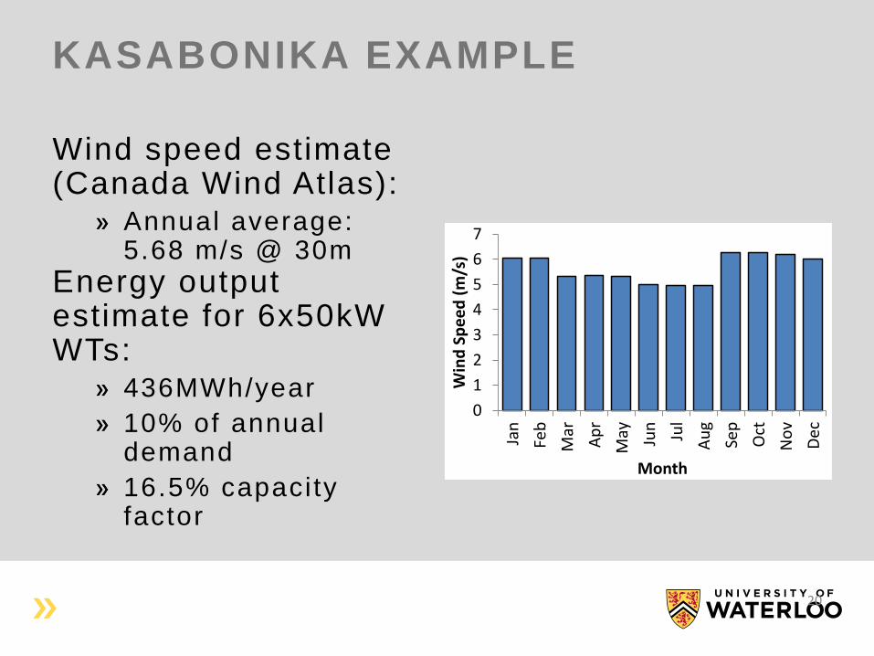
KASABONIKA EXAMPLE
Wind speed estimate (Canada Wind Atlas):
Annual average: 5.68 m/s @ 30m
Energy output estimate for 6x50kW WTs:
436MWh/year
10% of annual demand
16.5% capacity factor
20
0
1
2
3
4
5
6
7
Jan
Feb
Mar
Ap
r
May Jun
Jul
Au
g
Sep
Oct
No
v
Dec
Win
d S
pe
ed
(m
/s)
Month
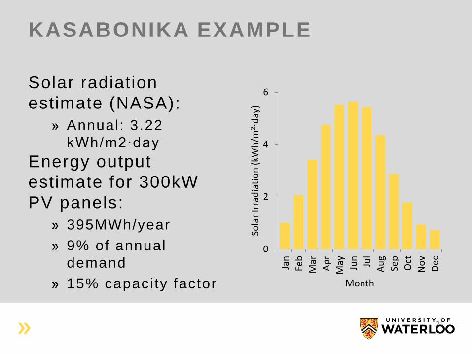
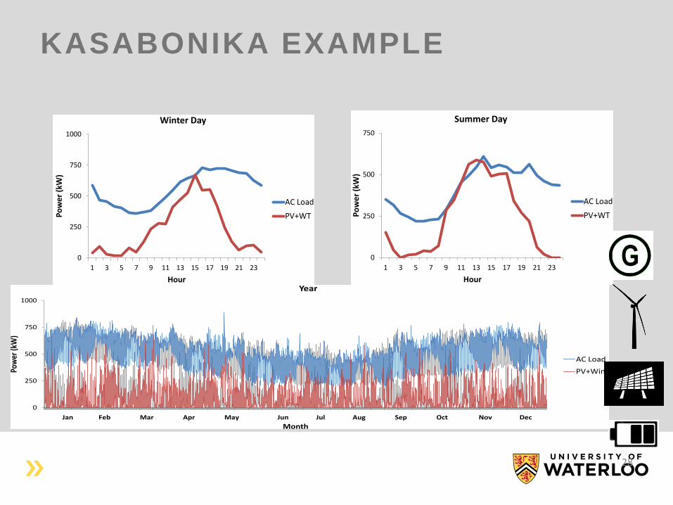
KASABONIKA EXAMPLE
Solar radiation
estimate (NASA):
Annual: 3.22
kWh/m2∙day
Energy output
estimate for 300kW
PV panels:
395MWh/year
9% of annual
demand
15% capacity factor
21
0
2
4
6
Jan
Feb
Mar
Ap
r
May Jun
Jul
Au
g
Sep
Oct
No
v
Dec
Sola
r Ir
rad
iati
on
(kW
h/m
2∙d
ay)
Month
KASABONIKA EXAMPLE
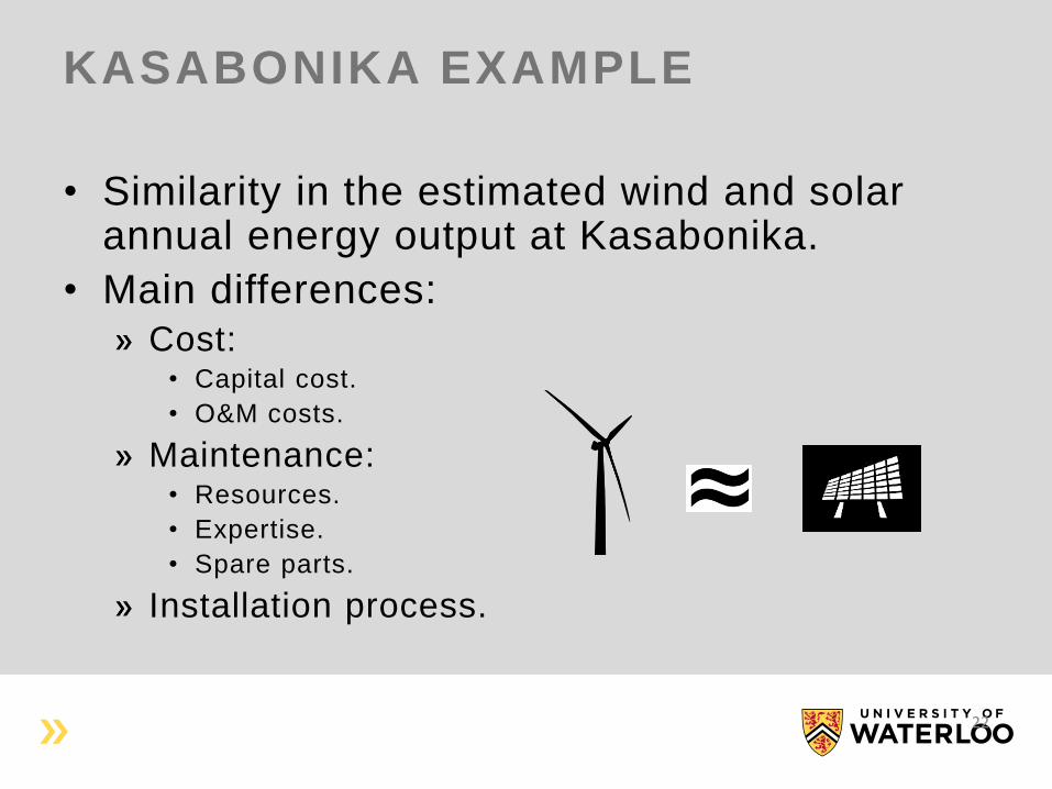
• Similarity in the estimated wind and solar annual energy output at Kasabonika.
• Main differences: Cost:
• Capital cost.
• O&M costs.
Maintenance: • Resources.
• Expertise.
• Spare parts.
Installation process.
22
KASABONIKA EXAMPLE
• Ranked sizing criteria for Wind/PV/DGS
option:
1. Wind/PV generation mix.
2. High RE penetration without excess energy.
3. Lower O&M costs within RE penetration range.
4. Lower capital cost than DGS upgrade.
23
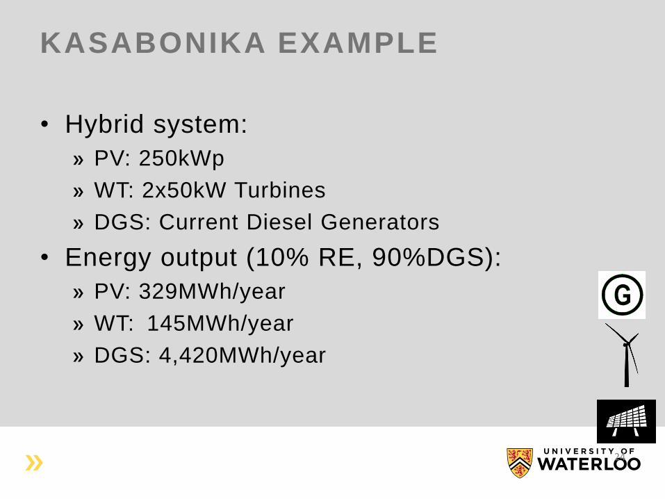
KASABONIKA EXAMPLE
• Hybrid system:
PV: 250kWp
WT: 2x50kW Turbines
DGS: Current Diesel Generators
• Energy output (10% RE, 90%DGS):
PV: 329MWh/year
WT: 145MWh/year
DGS: 4,420MWh/year
24
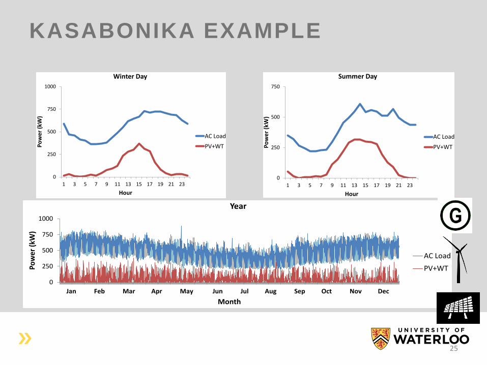
KASABONIKA EXAMPLE
25
0
250
500
750
1000
1 3 5 7 9 11 13 15 17 19 21 23
Po
we
r (k
W)
Hour
Winter Day
AC Load
PV+WT
0
250
500
750
1 3 5 7 9 11 13 15 17 19 21 23
Po
we
r (k
W)
Hour
Summer Day
AC Load
PV+WT
0
250
500
750
1000
Jan Sep Jun Mar Dec Sep Jun Mar Nov
Po
wer
(kW
)
Month
Year
AC Load
PV+WT
Jan Feb Mar Apr May Jun Jul Aug Sep Oct Nov Dec
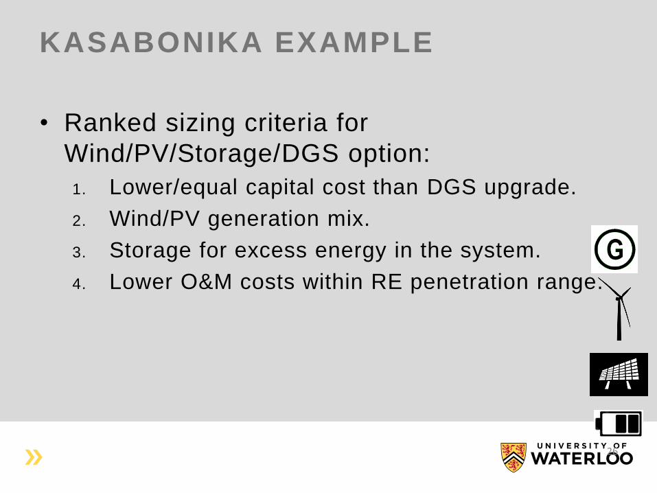
KASABONIKA EXAMPLE
• Ranked sizing criteria for
Wind/PV/Storage/DGS option:
1. Lower/equal capital cost than DGS upgrade.
2. Wind/PV generation mix.
3. Storage for excess energy in the system.
4. Lower O&M costs within RE penetration range.
26
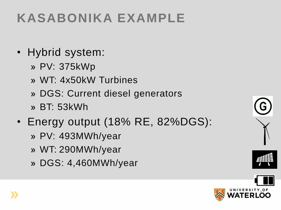
KASABONIKA EXAMPLE
• Hybrid system:
PV: 375kWp
WT: 4x50kW Turbines
DGS: Current diesel generators
BT: 53kWh
• Energy output (18% RE, 82%DGS):
PV: 493MWh/year
WT: 290MWh/year
DGS: 4,460MWh/year
27
0
250
500
750
1 3 5 7 9 11 13 15 17 19 21 23
Po
we
r (k
W)
Hour
Summer Day
AC Load
PV+WT
KASABONIKA EXAMPLE
0
250
500
750
1000
1 3 5 7 9 11 13 15 17 19 21 23
Po
we
r (k
W)
Hour
Winter Day
AC Load
PV+WT
0
250
500
750
1000
1 1001 2001 3001 4001 5001 6001 7001 8001
Pow
er (k
W)
Month
Year
AC Load
PV+Wind
Jan Feb Mar Apr May Jun Jul Aug Sep Oct Nov Dec
28
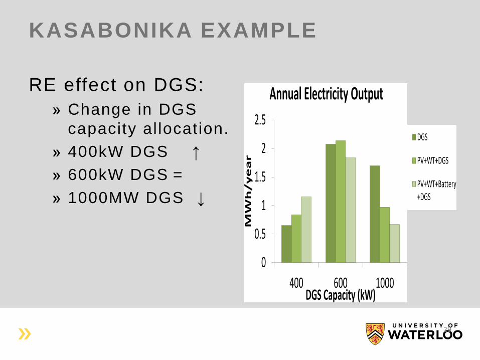
KASABONIKA EXAMPLE
RE effect on DGS:
Change in DGS
capacity allocation.
400kW DGS ↑
600kW DGS =
1000MW DGS ↓
29
0
500
1000
1500
2000
2500
400 600 1000
kW
h/y
ea
r
DGS Capacity (kW)
Annual Electricity Output
DGS
PV+WT+DGS
PV+WT+Battery+DGS
0
0.5
1
1.5
2
2.5
400 600 1000
MW
h/y
ea
r
DGS Capacity (kW)
Annual Electricity Output
KASABONIKA EXAMPLE
30
0
500
1000
1500
2000
2500
400 600 1000
kWh
/ye
ar
DGS Capacity (kW)
Annual Electricity Output
DGS
PV+WT+DGS
PV+WT+Battery+DGS
0
5
10
15
20
25
30
400 600 1000
Year
s
DGS Capacity (kW)
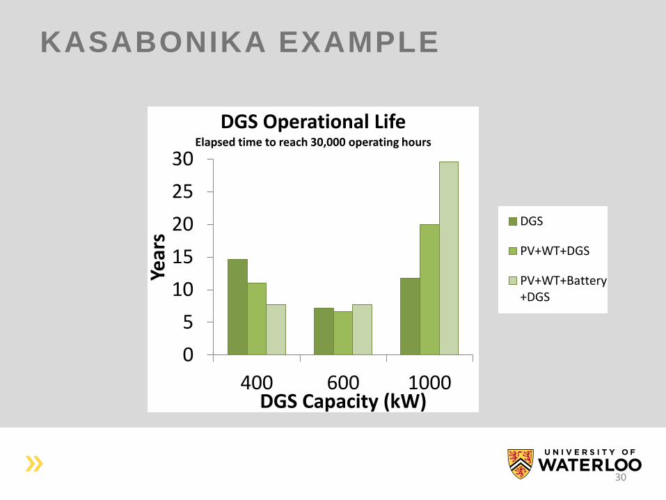
DGS Operational LifeElapsed time to reach 30,000 operating hours
KASABONIKA EXAMPLE
WT cost estimate:
Capital cost:
$9,250/kW
O&M cost:
$250/kW·year
3.5% of capital
cost
31
Turbine 59%
Foundation, electrical
installation, control
13%
Others 6%
Transport. 6%
Installation 3%
Conting. 13%
Capital Cost Breakdown
KASABONIKA EXAMPLE
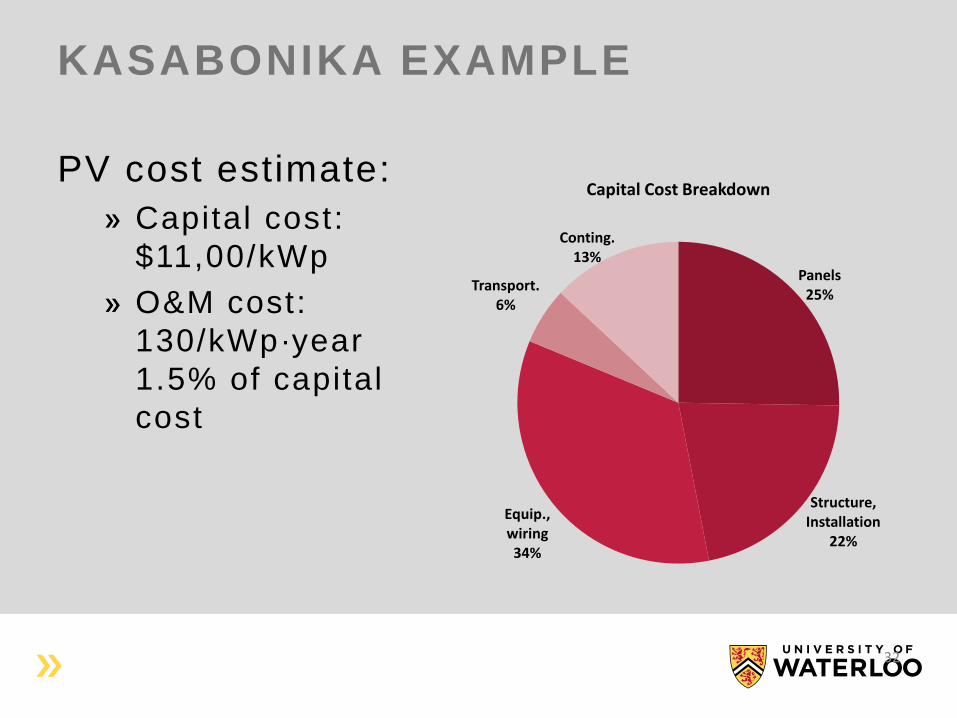
PV cost estimate:
Capital cost:
$11,00/kWp
O&M cost:
130/kWp·year
1.5% of capital
cost
32
Panels 25%
Structure, Installation
22%
Equip., wiring 34%
Transport. 6%
Conting. 13%
Capital Cost Breakdown
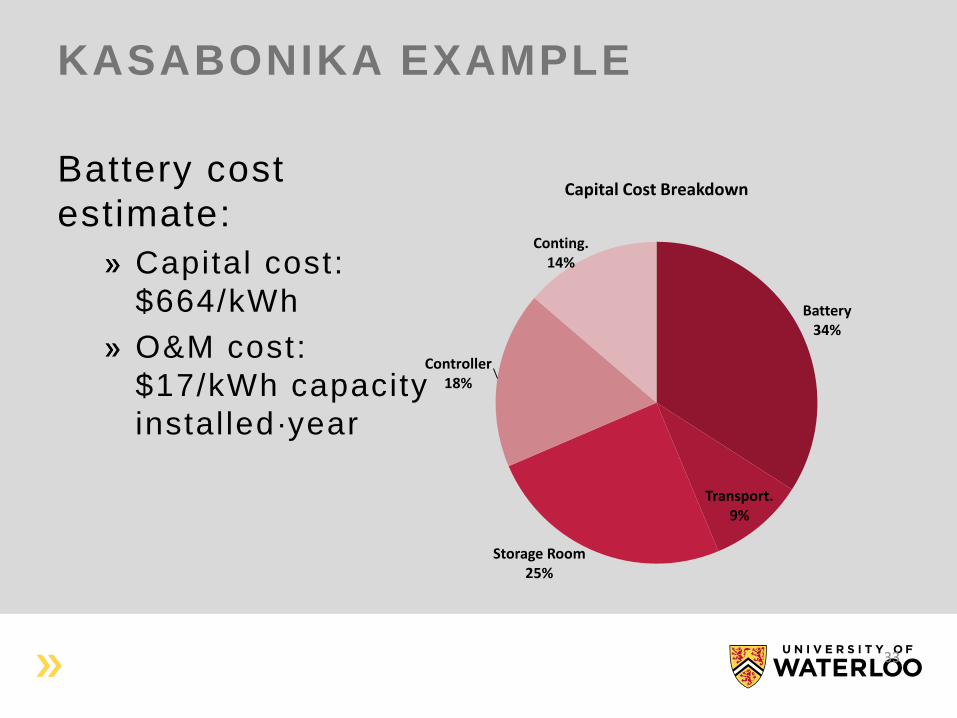
KASABONIKA EXAMPLE
Battery cost
estimate:
Capital cost:
$664/kWh
O&M cost:
$17/kWh capacity
installed·year
Battery 34%
Transport. 9%
Storage Room 25%
Controller 18%
Conting. 14%
Capital Cost Breakdown
33
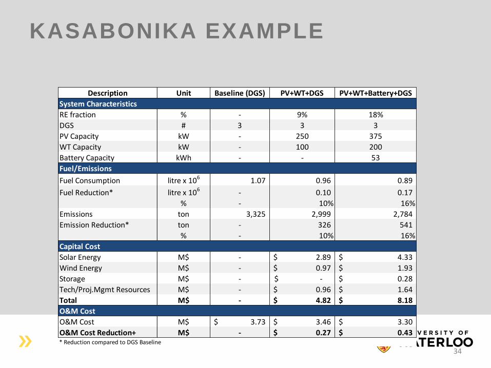
KASABONIKA EXAMPLE
34
Description Unit Baseline (DGS) PV+WT+DGS PV+WT+Battery+DGS
System Characteristics
RE fraction % - 9% 18%
DGS # 3 3 3
PV Capacity kW - 250 375
WT Capacity kW - 100 200
Battery Capacity kWh - - 53
Fuel/Emissions
Fuel Consumption litre x 106 1.07 0.96 0.89
Fuel Reduction* litre x 106 - 0.10 0.17
% - 10% 16%
Emissions ton 3,325 2,999 2,784
Emission Reduction* ton - 326 541
% - 10% 16%
Capital Cost
Solar Energy M$ - 2.89$ 4.33$
Wind Energy M$ - 0.97$ 1.93$
Storage M$ - -$ 0.28$
Tech/Proj.Mgmt Resources M$ - 0.96$ 1.64$
Total M$ - 4.82$ 8.18$
O&M Cost
O&M Cost M$ 3.73$ 3.46$ 3.30$
O&M Cost Reduction+ M$ - 0.27$ 0.43$ * Reduction compared to DGS Baseline
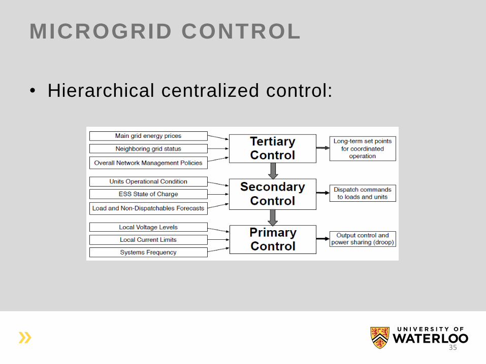
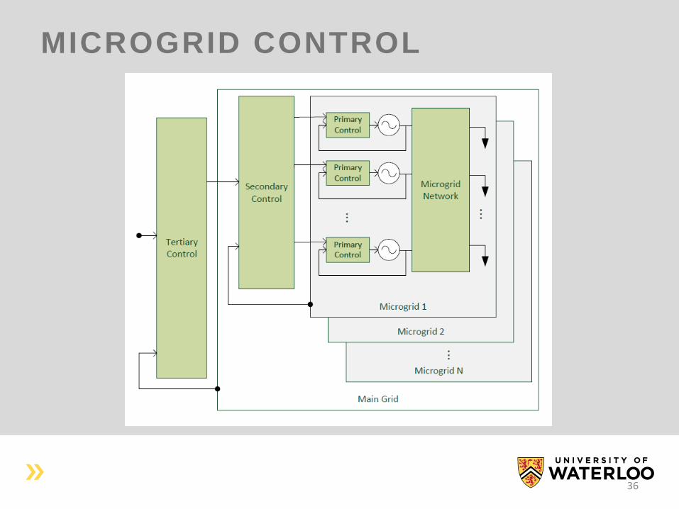
MICROGRID CONTROL
• Hierarchical centralized control:
35
MICROGRID CONTROL
36
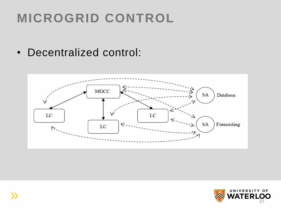
MICROGRID CONTROL
• Decentralized control:
37
MICROGRID CONTROL
• Grid-connected microgrids:
V and particularly f control is not a major issue,
as the grid provides these “services”.
DGs on PQ control mode is the current
“standard” in this case, including non-
dispatchable DGs (solar PV and some wind
generators).
V control is being considered/implemented by
LDCs when DGs allow (e.g. solar PV).
38
MICROGRID CONTROL
• Isolated (e.g. remote) microgrids:
V and f control are a major issue and must be
implemented.
V control is prevalent in most DG technologies.
F control is available and “dependable” only in
diesel generators, microturbines/CHP turbines
and energy (battery) storage systems.
39
MICROGRID CONTROL
• As more DGs of various technologies are
added to microgrids (on- or off-grid), the
need to coordinate controls is important:
Primary controls are based on droops to
“allocate” control, as in large grids.
Secondary controls: • Hierarchical, centralized controls similar to those found in
large grids (e.g. SVR, AGC).
• Distributed controls: – Agent based controls.
– Distributed OPF approaches.
40
MICROGRID CONTROL
Tertiary controls: • The main objective is to optimize the control with an
“overall” (central or distributed) optimization of the grid.
• Not widely implemented in large grids in practice, where is
only applied to V control.
• It can be viewed as optimal control coordination of multiple
microgrids and their common grid.
41
MICROGRID CONTROL
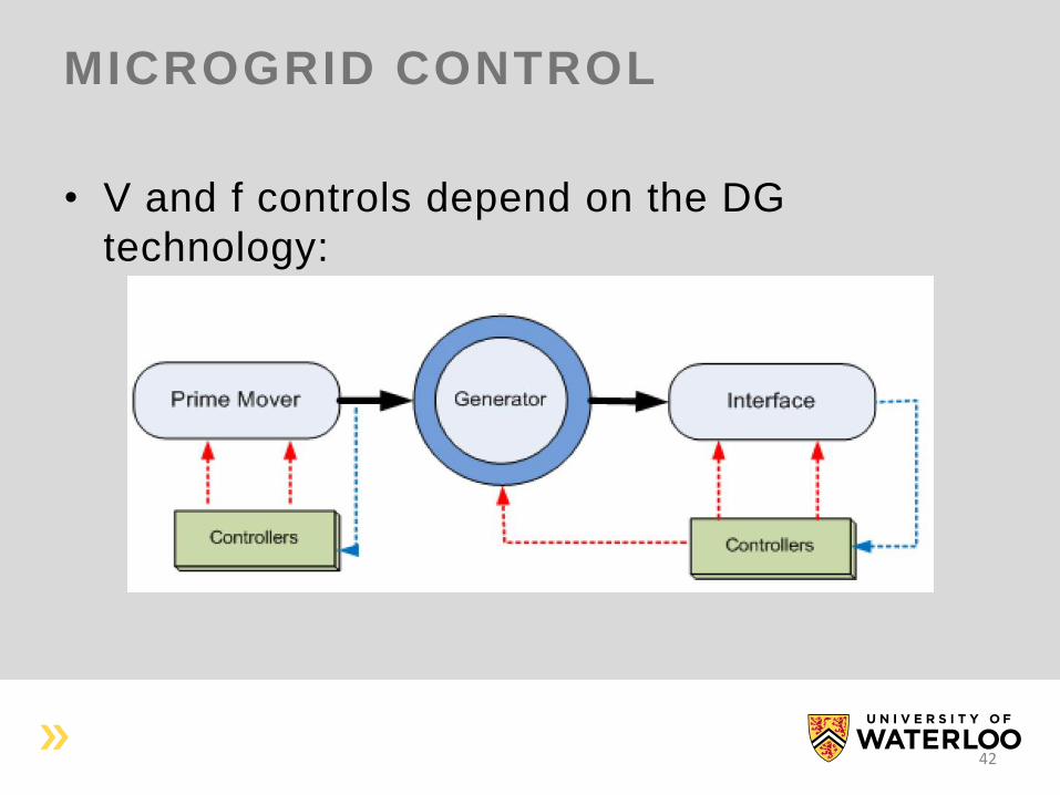
• V and f controls depend on the DG
technology:
42
MICROGRID CONTROL
• V controls:
Available in diesel gen. sets, microturbines, CHP
turbines, VSC-based DGs (solar PV, some wind
generators, fuel cells), DFIG-based wind
generators (usually found in farms and not
“individually” as part of microgrids), battery
storage systems.
Not available in IM-based wind turbines (old, but
somewhat prevalent technology in remote, small
microgrids).
43
V AND F CONTROL
• F controls:
Available and dependable in diesel gen. sets,
microturbines/CHP turbines and battery storage
systems, given their dispatchability and relatively
fast response.
Not available in non-dispatchable sources, i.e.
solar PV, wind, small hydro.
44
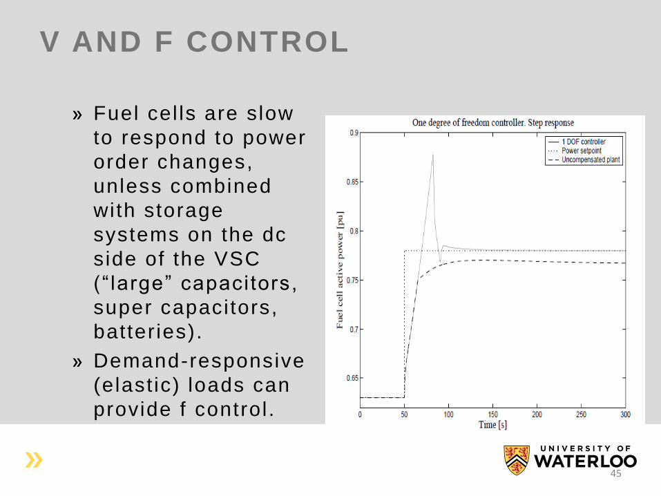
V AND F CONTROL
Fuel cel ls are slow
to respond to power
order changes,
unless combined
with storage
systems on the dc
side of the VSC
(“ large” capacitors,
super capacitors,
batter ies).
Demand-responsive
(elast ic) loads can
provide f control .
45
V AND F CONTROL
46
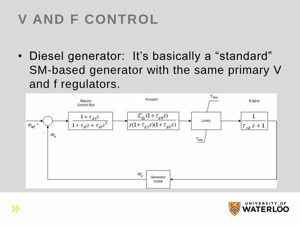
• Diesel generator: It’s basically a “standard”
SM-based generator with the same primary V
and f regulators.
V AND F CONTROL
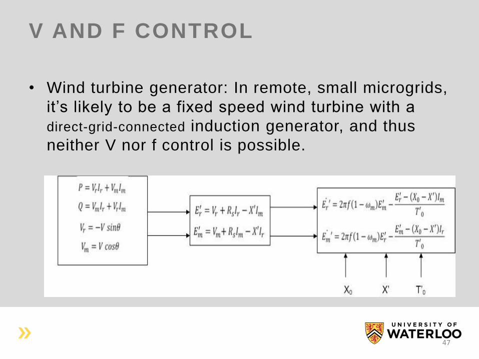
• Wind turbine generator: In remote, small microgrids,
it’s likely to be a fixed speed wind turbine with a
direct-grid-connected induction generator, and thus
neither V nor f control is possible.
47
V AND F CONTROL
48
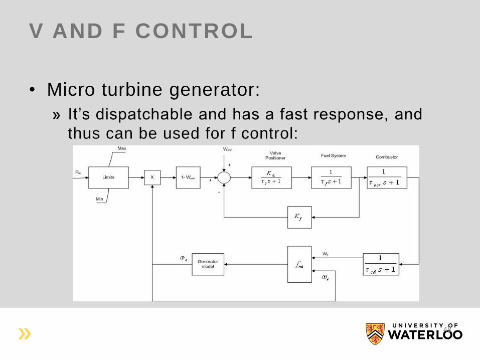
• Micro turbine generator:
It’s dispatchable and has a fast response, and
thus can be used for f control:
V AND F CONTROL
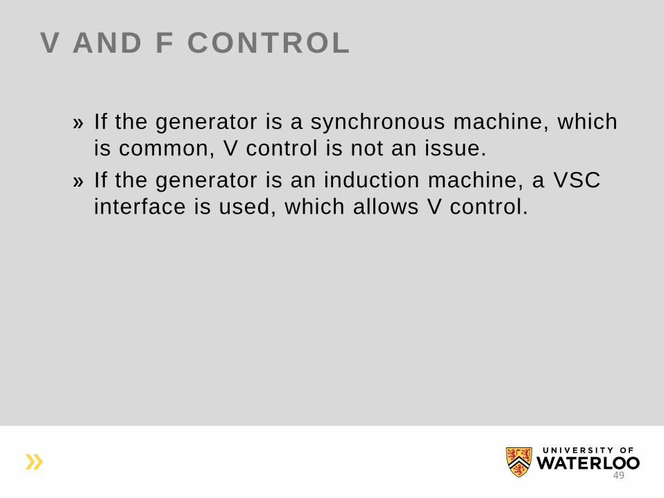
If the generator is a synchronous machine, which
is common, V control is not an issue.
If the generator is an induction machine, a VSC
interface is used, which allows V control.
49
V AND F CONTROL
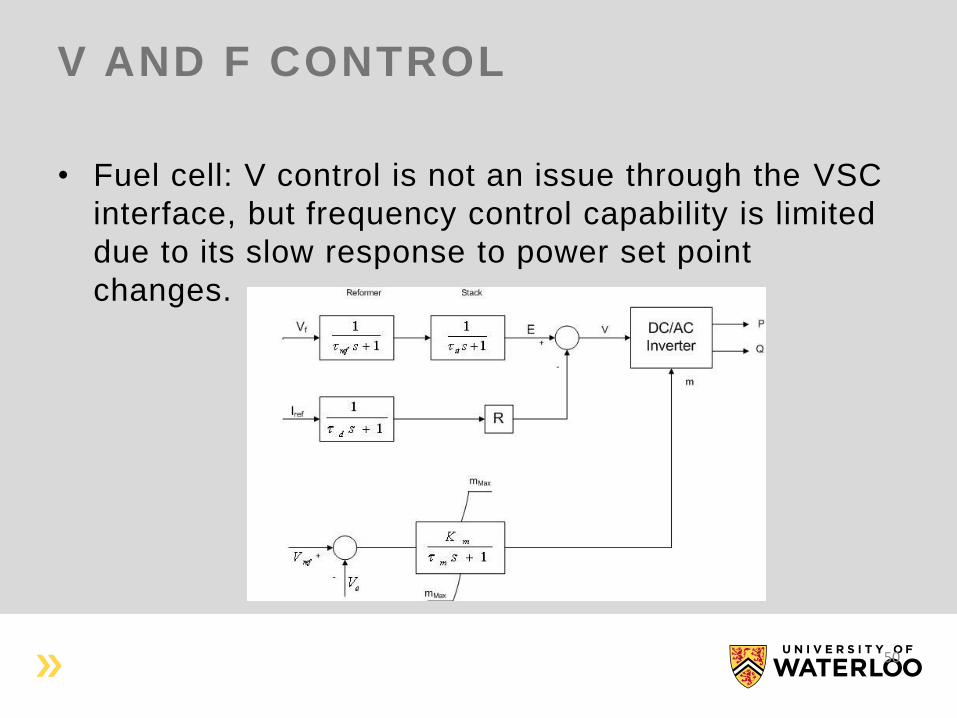
• Fuel cell: V control is not an issue through the VSC
interface, but frequency control capability is limited
due to its slow response to power set point
changes.
50
V AND F CONTROL
51
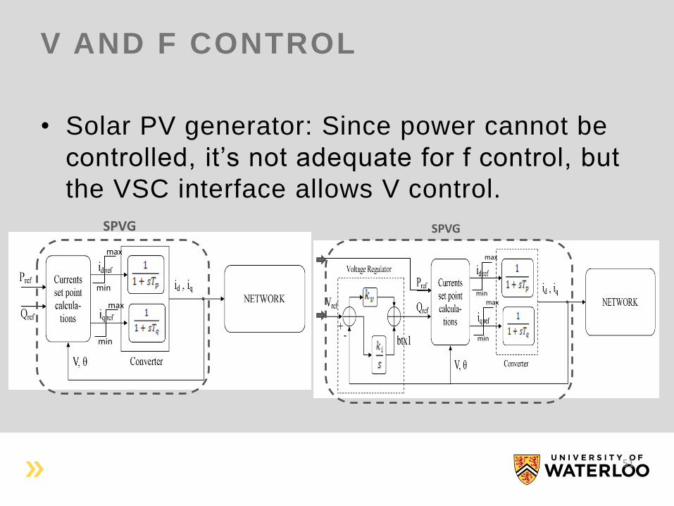
• Solar PV generator: Since power cannot be
controlled, it’s not adequate for f control, but
the VSC interface allows V control.
SPVG
max
min
max
min
max
min max
min
SPVG
ENERGY MANAGEMENT PROBLEM
• An Energy Management System (EMS) is a set of protocols and computer applications designed to assist power system operators in the operation of the grid.
• There computer applications incorporate online data analysis and include:
State estimation.
OPF.
Voltage control/reactive power optimization.
Security assessment.
Load forecasting.
52
ENERGY MANAGEMENT PROBLEM
• In microgrids, all the EMS applications must
be performed by an autonomous automated
system as part of the secondary control
level.
• The operation of an EMS in a microgrid
becomes more challenging due to the critical
demand-supply balance, low inertia of the
system and the presence of energy storage
systems.
53
ENERGY MANAGEMENT PROBLEM
• The general EMS case: Find the optimal or near optimal unit commitment of units.
Find the optimal or near optimal dispatch of units.
Find the optimal or near optimal voltage settings.
• Challenges for EMS in microgrids: Intermittent and hard to predict generation.
System states are coupled in time due to Unit Commitment (UC) decisions and Energy Storage Systems (ESS).
Multiple objectives (e.g. total cost, GHG emissions)
Multiple owners and sometimes conflicting objectives.
54
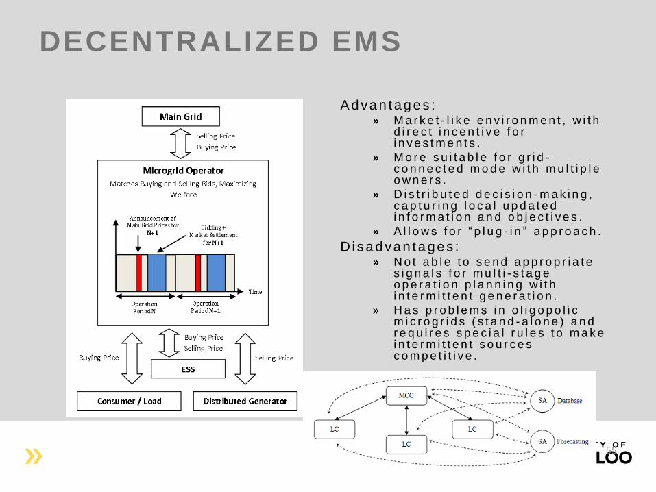
DECENTRALIZED EMS
Ad va n ta g e s : M a r k e t - l i k e e n v i r o n m e n t , w i t h d i r e c t i n c e n t i v e f o r i n v e s t m e n t s .
M o r e s u i t a b l e f o r g r i d -c o n n e c t e d m o d e w i t h m u l t i p l e o w n e r s .
D i s t r i b u t e d d e c i s i o n - m a k i n g , c a p t u r i n g l o c a l u p d a t e d i n f o r m a t i o n a n d o b j e c t i v e s .
A l l o w s f o r “ p l u g - i n ” a p p r o a c h .
Dis advan tages : N o t a b l e t o s e n d a p p r o p r i a t e s i g n a l s f o r m u l t i - s t a g e o p e r a t i o n p l a n n i n g w i t h i n t e r m i t t e n t g e n e r a t i o n .
H a s p r o b l e m s i n o l i g o p o l i c m i c r o g r i d s ( s t a n d - a l o n e ) a n d r e q u i r e s s p e c i a l r u l e s t o m a k e i n t e r m i t t e n t s o u r c e s c o m p e t i t i v e .
55
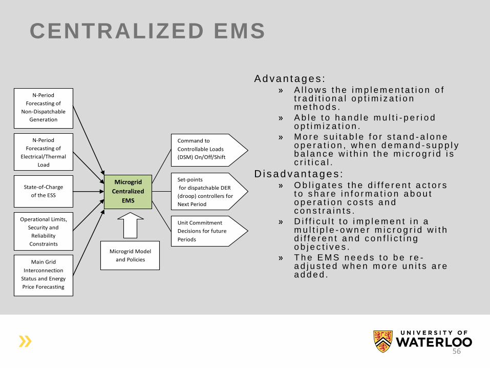
CENTRALIZED EMS
N-Period
Forecasting of
Non-Dispatchable
Generation
Microgrid
Centralized
EMS
State-of-Charge
of the ESS
Microgrid Model
and Policies
N-Period
Forecasting of
Electrical/Thermal
Load
Operational Limits,
Security and
Reliability
Constraints
Command to
Controllable Loads
(DSM) On/Off/Shift
Set-points
for dispatchable DER
(droop) controllers for
Next Period
Unit Commitment
Decisions for future
Periods
Main Grid
Interconnection
Status and Energy
Price Forecasting
Ad va n ta g e s : A l l o w s t h e i m p l e m e n t a t i o n o f t r a d i t i o n a l o p t i m i z a t i o n m e t h o d s .
A b l e t o h a n d l e m u l t i - p e r i o d o p t i m i z a t i o n .
M o r e s u i t a b l e f o r s t a n d - a l o n e o p e r a t i o n , w h e n d e m a n d - s u p p l y b a l a n c e w i t h i n t h e m i c r o g r i d i s c r i t i c a l .
Dis a d va n ta ge s : O b l i g a t e s t h e d i f f e r e n t a c t o r s t o s h a r e i n f o r m a t i o n a b o u t o p e r a t i o n c o s t s a n d c o n s t r a i n t s .
D i f f i c u l t t o i m p l e m e n t i n a m u l t i p l e - o w n e r m i c r o g r i d w i t h d i f f e r e n t a n d c o n f l i c t i n g o b j e c t i v e s .
T h e E M S n e e d s t o b e r e -a d j u s t e d w h e n m o r e u n i t s a r e a d d e d .
56
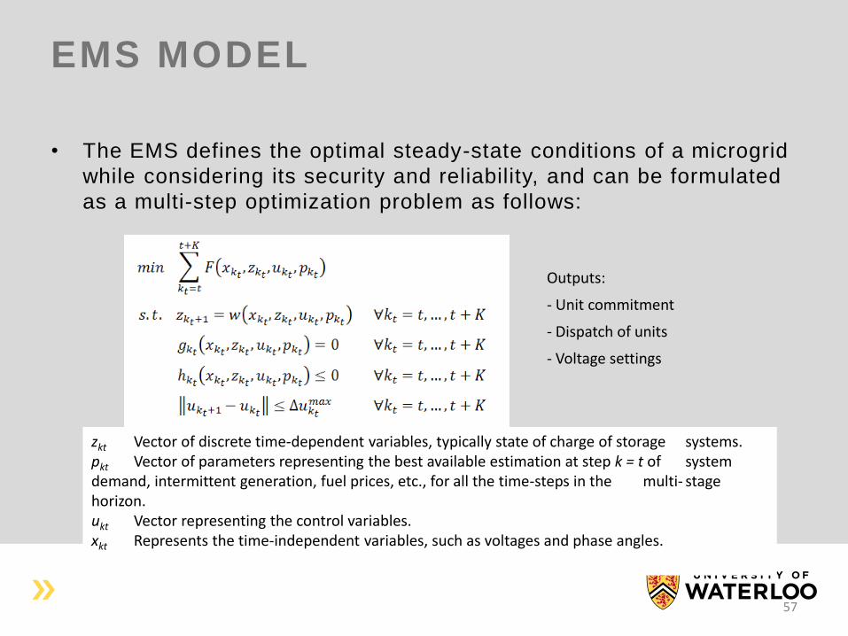
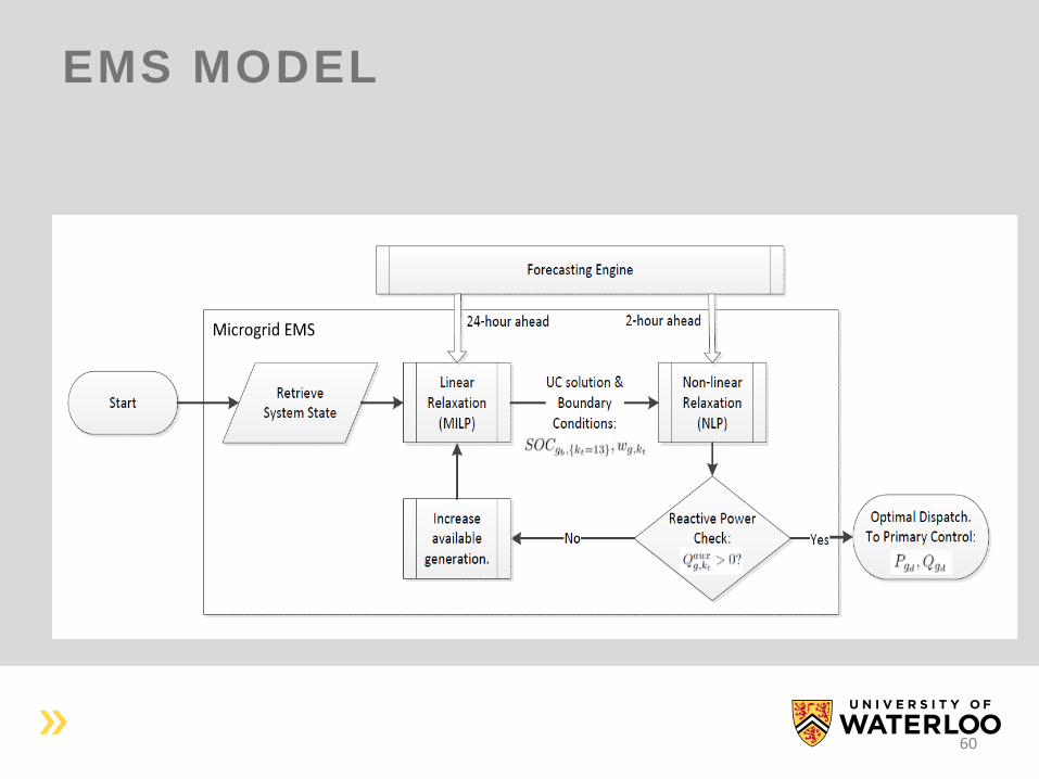
EMS MODEL
• The EMS defines the optimal steady-state conditions of a microgrid
while considering its security and reliability, and can be formulated
as a multi-step optimization problem as follows:
zkt Vector of discrete time-dependent variables, typically state of charge of storage systems. pkt Vector of parameters representing the best available estimation at step k = t of system demand, intermittent generation, fuel prices, etc., for all the time-steps in the multi- stage horizon. ukt Vector representing the control variables. xkt Represents the time-independent variables, such as voltages and phase angles.
Outputs:
- Unit commitment
- Dispatch of units
- Voltage settings
57
EMS MODEL
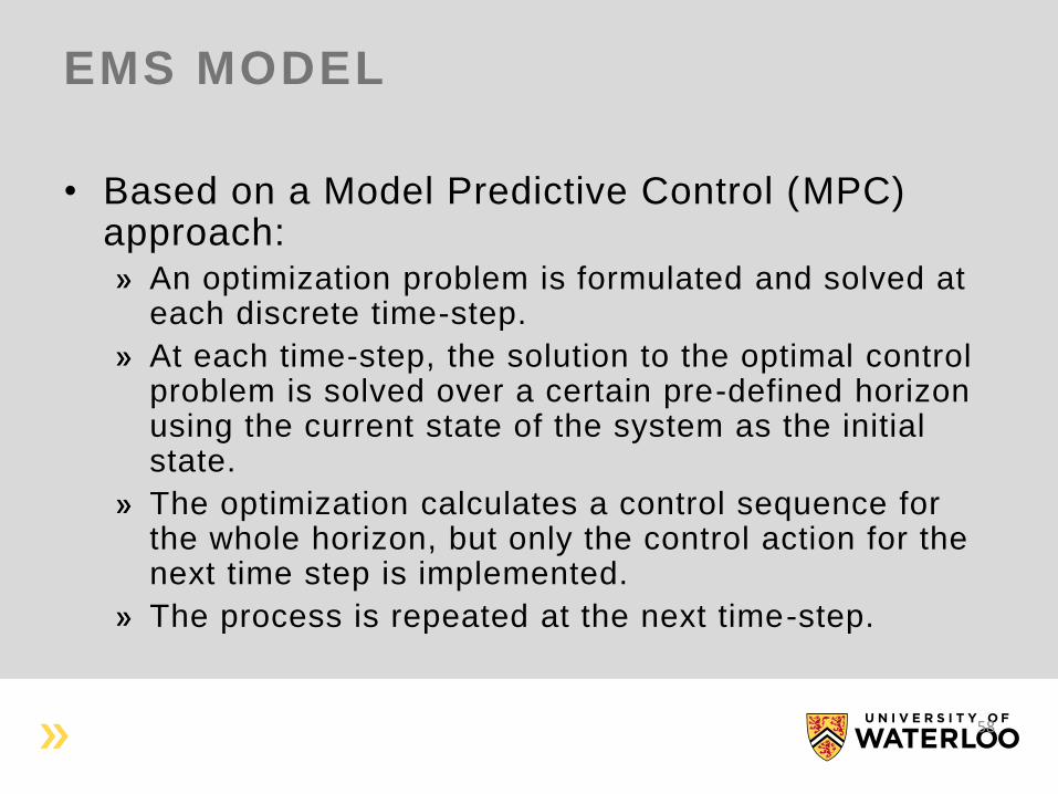
• Based on a Model Predictive Control (MPC) approach:
An optimization problem is formulated and solved at each discrete time-step.
At each time-step, the solution to the optimal control problem is solved over a certain pre-defined horizon using the current state of the system as the initial state.
The optimization calculates a control sequence for the whole horizon, but only the control action for the next time step is implemented.
The process is repeated at the next time-step.
58
EMS MODEL
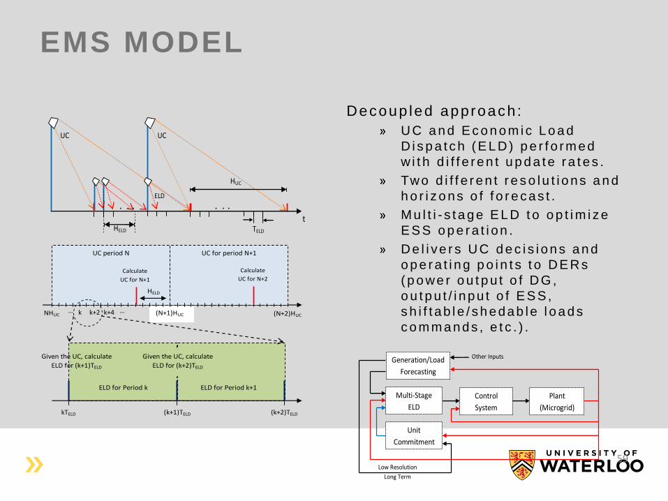
Decoup led approach:
U C a n d E c o n om i c L o a d
D i s p a t c h ( E L D ) p e r f o rm ed
w i t h d i f f e ren t u p d a t e r a t es .
Two d i f f e r en t r e s o lu t i o ns a n d
h o r i z o ns o f f o r e c as t .
M u l t i - s t a ge E L D t o o p t i m i z e
E S S o p e r a t i on .
D e l i ve r s U C d e c i s i on s a n d
o p e r a t i ng p o i n t s t o D E R s
( p o we r o u t p u t o f D G ,
o u t p u t / i npu t o f E S S ,
s h i f t ab l e / s h edab le l o a d s
c o m m a nds , e t c . ) .
59
Unit
Commitment
Multi-Stage
ELD
Control
System
Plant
(Microgrid)
Generation/Load
Forecasting
Other Inputs
Low Resolution
Long Term
ELD
t
UC UC
. . . . . .
HELD
HUC
TELD
k
ELD for Period k ELD for Period k+1
Given the UC, calculate
ELD for (k+2)TELD
Given the UC, calculate
ELD for (k+1)TELD
kTELD (k+1)TELD (k+2)TELD
(N+2)HUC NHUC (N+1)HUC
UC period N UC for period N+1
Calculate
UC for N+1
Calculate
UC for N+2
HELD
k+4 k+2 … …
EMS MODEL
60
EMS MODEL
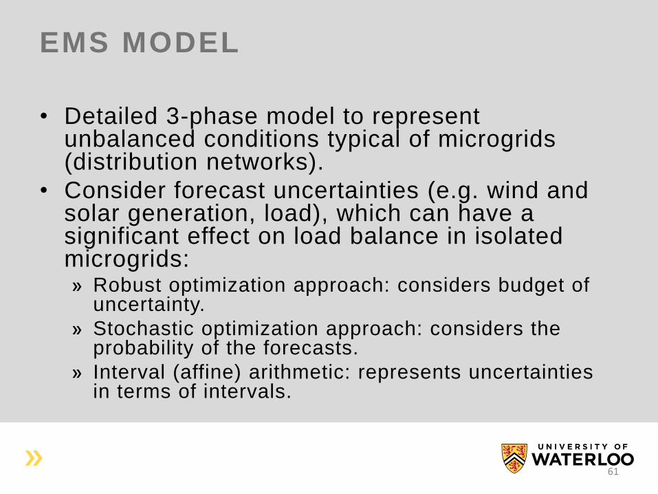
• Detailed 3-phase model to represent unbalanced conditions typical of microgrids (distribution networks).
• Consider forecast uncertainties (e.g. wind and solar generation, load), which can have a significant effect on load balance in isolated microgrids:
Robust optimization approach: considers budget of uncertainty.
Stochastic optimization approach: considers the probability of the forecasts.
Interval (affine) arithmetic: represents uncertainties in terms of intervals.
61
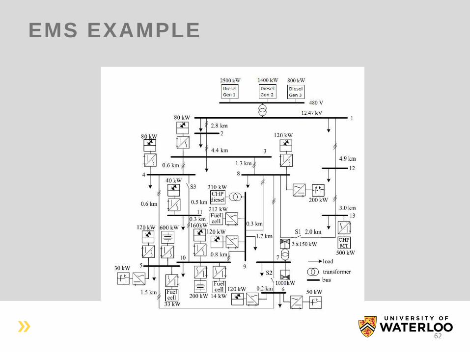
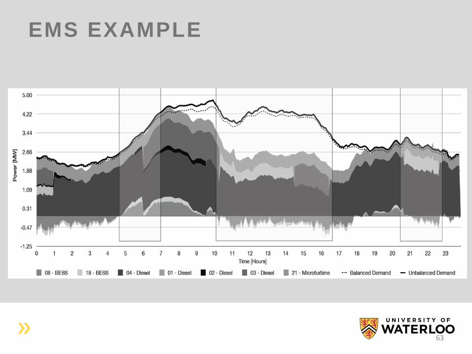
EMS EXAMPLE
62
EMS EXAMPLE
63
STABILITY
• There is a lack of understanding of the
dynamics of DGs under unbalanced
conditions.
• A full characterization of the unbalanced
system in stability analyses allows a better
understanding of dynamic behaviour of DGs.
• Most DGs nowadays are equipped with small
synchronous generators (e.g., diesel
generators, microturbines)
64
STABILITY
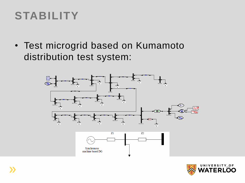
• Test microgrid based on Kumamoto
distribution test system:
65
Bus9Bus8Bus7
Bus6
Bus5
Bus4
Bus3
Bus2
Bus16
Bus15
Bus14
Bus13
Bus12
Bus11
Bus10
Bus1
STABILITY
• Stability studies:
Voltage stability studies based on P-V and P-L
curves.
Transient stability studies based on time domain
simulations to study contingencies.
Small perturbation stability studies using a model
identification approach to compute the
eigenvalues.
66
VOLTAGE STABILITY
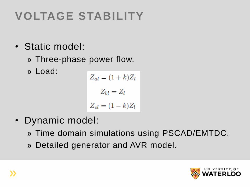
• Static model:
Three-phase power flow.
Load:
• Dynamic model:
Time domain simulations using PSCAD/EMTDC.
Detailed generator and AVR model.
67
VOLTAGE STABILITY
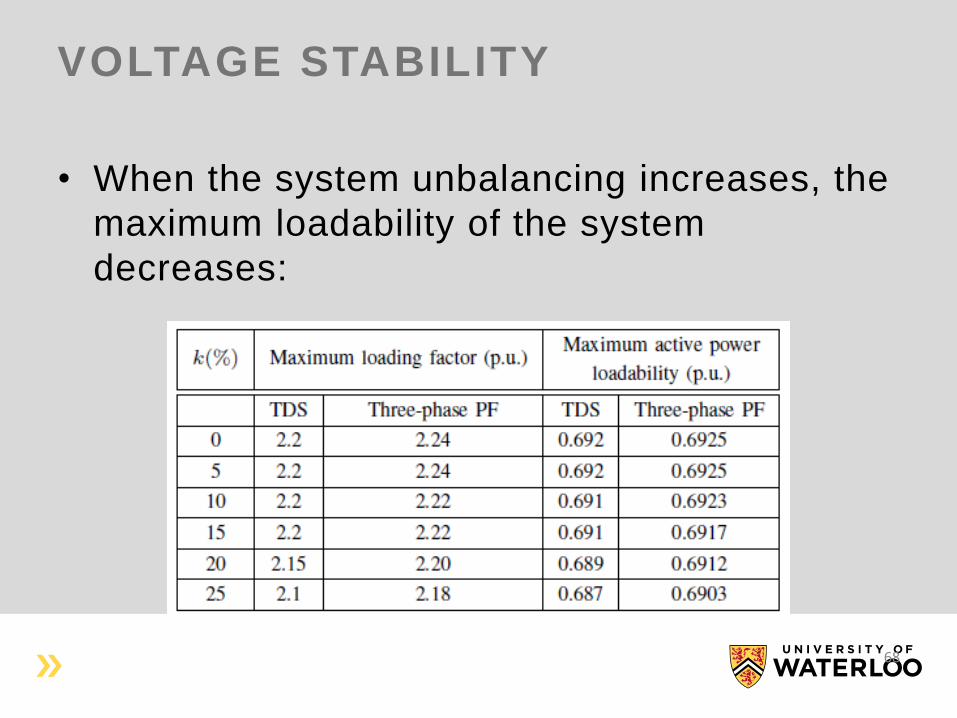
• When the system unbalancing increases, the
maximum loadability of the system
decreases:
68
VOLTAGE STABILITY
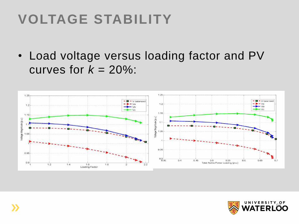
• Load voltage versus loading factor and PV
curves for k = 20%:
69
TRANSIENT STABILITY
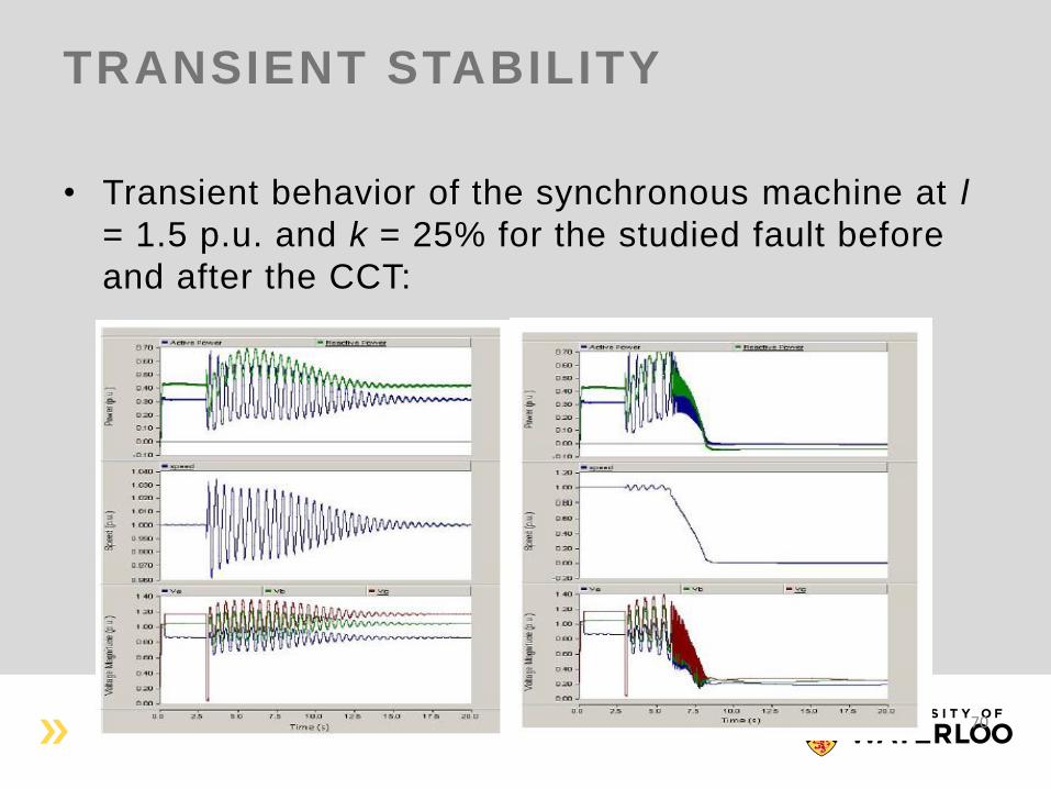
• Transient behavior of the synchronous machine at l
= 1.5 p.u. and k = 25% for the studied fault before
and after the CCT:
70
TRANSIENT STABILITY
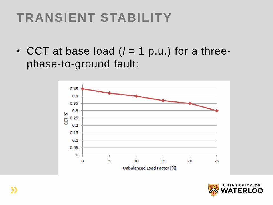
• CCT at base load (l = 1 p.u.) for a three-
phase-to-ground fault:
71
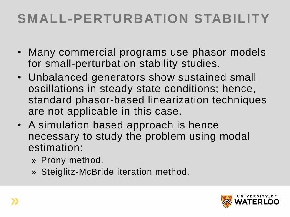
SMALL-PERTURBATION STABILITY
• Many commercial programs use phasor models for small-perturbation stability studies.
• Unbalanced generators show sustained small oscillations in steady state conditions; hence, standard phasor-based linearization techniques are not applicable in this case.
• A simulation based approach is hence necessary to study the problem using modal estimation:
Prony method.
Steiglitz-McBride iteration method.
72
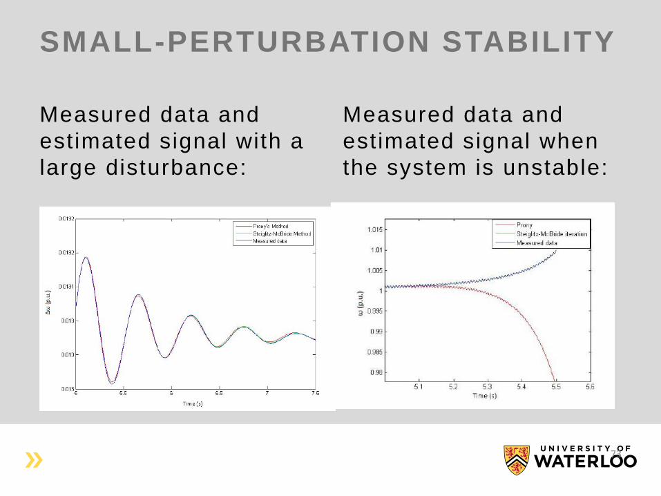
SMALL-PERTURBATION STABILITY
Measured data and
estimated signal with a
large disturbance:
Measured data and
estimated signal when
the system is unstable:
73
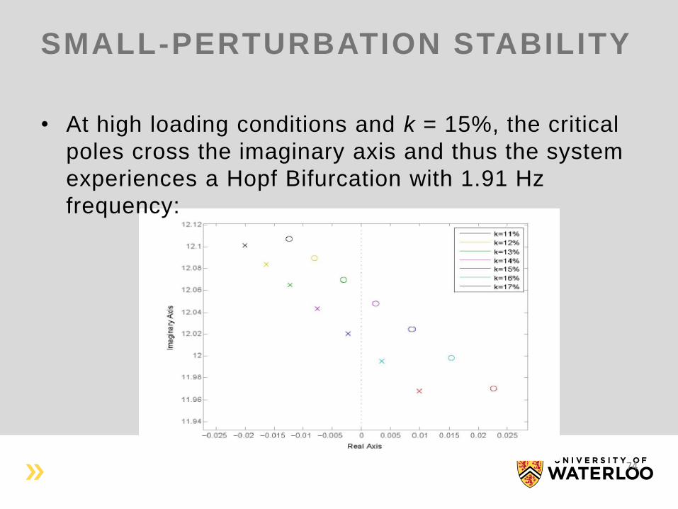
SMALL-PERTURBATION STABILITY
• At high loading conditions and k = 15%, the critical
poles cross the imaginary axis and thus the system
experiences a Hopf Bifurcation with 1.91 Hz
frequency:
74
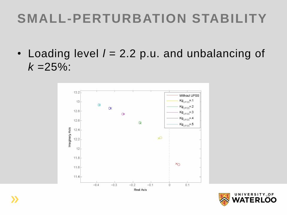
SMALL-PERTURBATION STABILITY
• Loading level l = 2.2 p.u. and unbalancing of
k =25%:
75
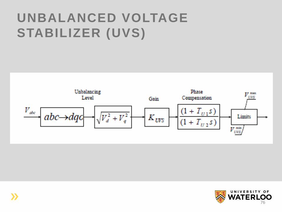
UNBALANCED VOLTAGE
STABILIZER (UVS)
76
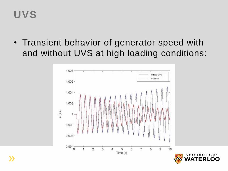
UVS
• Transient behavior of generator speed with
and without UVS at high loading conditions:
77


![Coordination Control Strategy for AC/DC Hybrid Microgrids in ......AC and DC microgrids is proposed, and this emerges the concept of hybrid AC/DC microgrids [5,6]. Control of microgrids](https://img.pdfslide.us/doc/110x75/61032ae7c5c5ba536268cbac/coordination-control-strategy-for-acdc-hybrid-microgrids-in-ac-and-dc-microgrids.jpg)