Embed Size (px)
Citation preview
HAL Id: tel-02077668https://tel.archives-ouvertes.fr/tel-02077668
Submitted on 23 Mar 2019
HAL is a multi-disciplinary open accessarchive for the deposit and dissemination of sci-entific research documents, whether they are pub-lished or not. The documents may come fromteaching and research institutions in France orabroad, or from public or private research centers.
L’archive ouverte pluridisciplinaire HAL, estdestinée au dépôt et à la diffusion de documentsscientifiques de niveau recherche, publiés ou non,émanant des établissements d’enseignement et derecherche français ou étrangers, des laboratoirespublics ou privés.
Sizing and Operation of Multi-Energy Hydrogen-BasedMicrogrids
Bei Li
To cite this version:Bei Li. Sizing and Operation of Multi-Energy Hydrogen-Based Microgrids. Electric power. UniversitéBourgogne Franche-Comté, 2018. English. �NNT : 2018UBFCA021�. �tel-02077668�
THESE DE DOCTORAT DE L’ETABLISSEMENT UNIVERSITE BOURGOGNE FRANCHE-COMTE
PREPAREE A L’UNIVERSITE DE TECHNOLOGIE DE BELFORT-MONTBELIARD
Ecole doctorale n°37
Sciences Pour l’Ingenieur et Microtechniques
Doctorat de Genie Electrique
par
BEI LI
Sizing and Operation of Multi-Energy Hydrogen-Based Microgrids
These presentee et soutenue a Belfort, le 24 septembre 2018
Composition du Jury :
IDOUMGHAR LHASSANE Professeur a l’Universite de HauteAlsace
President
ROBOAM XAVIER Directeur de Recherche CNRS al’Universite de Toulouse
Rapporteur
PIERFEDERICI SERGE Professeur a l’Universite de Lorraine RapporteurPRODAN IONELA Maıtre de Conferences a Grenoble INP ExaminatriceMIRAOUI ABDELLATIF Professeur a l’Universite de Technologie
de Belfort-MontbeliardDirecteur de these
ROCHE ROBIN Maıtre de Conferences a l’Universite deTechnologie de Belfort-Montbeliard
Co-encadrant
PAIRE DAMIEN Maıtre de Conferences a l’Universite deTechnologie de Belfort-Montbeliard
Co-encadrant


école doctorale sciences pour l ’ingénieur et microtechniques
Universite Bourgogne Franche-Comte32, avenue de l’Observatoire25000 Besanon, France

ABSTRACT
With the development of distributed, renewable energy sources, microgrids can be ex-pected to play an important role in future power systems, not only to reduce emissionsand maximize local energy use, but also to improve system resilience. Due to the inter-mittence and uncertainty of renewable sources (such as photovoltaics or wind turbines),energy storage systems should also be integrated. However, determining their size andhow to operate them remains challenging, especially as the adopted control strategyimpacts sizing results, and for systems considering multiple, interdependent forms of en-ergy. This thesis therefore contributes to solving the sizing and operation problems offull-electric and multi-energy (electricity, gas, heat, cooling and/or hydrogen) microgridsintegrating storage systems.
First, based on the characteristics of different components, a mathematical model of amicrogrid is built. Then, the operation problem is formulated as a mixed integer linearproblem (MILP), based on an objective function (minimize the operation cost) and dif-ferent constraints (maximum power, startup/shutdown times, state-of-charge limits, etc.).Next, a co-optimization structure is presented to solve the sizing problem using a ge-netic algorithm. This specific structure enables to search for sizing values based on theoperation results, which enables determining the best sizing for the selected operationstrategy.
Using the above method, four specific problems are then studied. The first one focuses onsizing a full-electric islanded microgrid combining battery and hydrogen storage systemsfor short and long-term storage, respectively. Results for two types of operation strategiesare compared: the MILP approach and a rule-based strategy. A one-hour one-year rollinghorizon simulation is used to check the validity of the sizing results.
Second, a multi-energy islanded microgrid with different types of loads is studied. Specif-ically, the influence of three factors on sizing results is analyzed: the operation strategy,the accuracy of load and renewable generation forecasts, and the degradation of energystorage systems.
Third, the work focuses on a grid-connected microgrid attached to a gas, electricity andheat hybrid network. Specifically, the resilience of the network is considered in order tomaximize resistance to contingency events. Betweenness centrality is used to find theworst case under contingency events and analyze their impact on sizing results. Two testsystems of different sizes are used with the proposed method and a study of its sensitivityto various parameters is carried out.
Fourth, a structure with multiple grid-connected multi-energy-supply microgrids is consid-ered, and an algorithm for determining electricity prices is developed. This price is usedfor energy exchanges between microgrids and load service entities interacting with theutility. The proposed co-optimization method is deployed to search for the best price thatmaximizes benefits to all players. Simulations on a large system show that the obtainedprice returns better results than a basic time-of-use price and helps reduce the operation
v

vi
cost of the whole system. To reduce the computation time, a neural network is presentedto estimate the operation of the whole system and enable obtaining results faster with alimited impact on performance. At last, a sizing algorithm for grid-connected multi-energysupply microgrids operating under different prices is presented.
The obtained results on these different applications show the usefulness of the proposedmethod, which is a promising contribution toward the creation of advanced design toolsfor such microgrids.
Keywords: microgrid, hydrogen, optimization, sizing, multi-energy, price.
RESUME
Avec le developpement de la production decentralisee d’electricite a partir de sourcesrenouvelables, il est fort probable que les micro-reseaux joueront un role central dans lesreseaux du futur, non seulement pour reduire les emissions de gaz a effet de serre etmaximiser l’utilisation d’energie produite localement, mais egalement pour ameliorer laresilience du systeme global. Du fait de l’intermittence et de l’incertitude sur la produc-tion renouvelable (par exemple, photovoltaıque ou eolien), des systemes de stockage del’energie doivent etre integres. Cependant, determiner leur dimensionnement et commentles controler pose plusieurs defis, en particulier parce que le dimensionnement optimaldepend de la strategie de gestion utilisee, ou encore lorsque differents types d’energiesont utilises. Cette these contribue a resoudre les problemes de dimensionnement etde gestion de micro-reseaux electriques et multi-energies (electricite, gaz, chaleur, froidet/ou hydrogene) integrant du stockage.
Tout d’abord, a l’aide des caracteristiques des differents composants, un modelemathematique de micro-reseau est developpe. Le probleme de sa gestion est ensuiteformule comme un probleme de programmation lineaire (MILP), utilisant une fonctionobjectif (minimiser le cout de fonctionnement) et differentes contraintes (puissance max-imum, duree de demarrage/arret, limites d’etat de charge, etc.). Ensuite, une structurepermettant une co-optimisation est presentee pour resoudre le probleme du dimension-nement a l’aide d’un algorithme genetique. Cette structure permet de explorer l’espacedes valeurs de dimensionnement en fonction des resultats de la strategie de gestion,ce qui permet de tendre vers le meilleur dimensionnement possible pour la strategieselectionnee.
A l’aide de la methode ci-dessus, quatre problemes specifiques sont etudies. Le premiers’interesse au dimensionnement d’un micro-reseau ılote entierement electrique, combi-nant stockage par batteries et hydrogene-energie pour du stockage a court et long terme,respectivement. Les resultats pour deux strategies de gestion sont compares : l’approcheproposee (MILP) et une strategie basee sur des regles. Une simulation a horizon glissantd’une heure sur un an est ensuite utilisee pour verifier la validite du dimensionnementobtenu.
Un second probleme s’interesse un a micro-reseau multi-energies ılote avec differentstypes de charges. L’influence de trois facteurs sur les resultats du dimensionnement esten particulier etudiee : la strategie de gestion, la precision des previsions de consomma-tion et de production renouvelable, ainsi que la degradation des moyens de stockage.
Une troisieme partie de la these traite du dimensionnement d’un micro-reseau connecteaux reseaux de gaz, electricite et chaleur. La resilience du reseau est etudiee de facon amaximiser la resistance a une panne ou un defaut. La notion de centralite intermediaireest utilisee pour determiner le cas le plus defavorable pour une contingence et analyserson impact sur le dimensionnement. Deux systemes de test de tailles differentes sontutilises pour valider l’application de la methode proposee et sa sensibilite a differents
vii

viii
parametres.
Enfin, une quatrieme application s’interesse a un ensemble de micro-reseaux multi-energies connectes entre eux et a un reseau principal. L’algorithme propose estalors applique a la determination du prix utilise pour les echanges d’energie entre lesmicro-reseaux et des fournisseurs de service en interaction avec le reseau principal.L’algorithme determine alors le prix qui maximise les benefices pour l’ensemble desparticipants. Des simulations sur un reseau montrent que le prix obtenu retourne demeilleurs resultats qu’une tarification classique de type heures creuses-heures pleineset permet de reduire le cout global de fonctionnement. Pour reduire le temps de cal-cul, un reseau de neurones est propose pour accelerer la modelisation de la gestion dusysteme et permet d’obtenir un gain de temps tout en ayant un impact limtie sur la perfor-mance. Enfin, un algorithme de dimensionnement pour les micro-reseaux multi-energiesconnectes au reseau a differents prix est presente.
Les resultats obtenus sur ces differentes applications montrent l’utilite de la methode pro-posee, qui constitue une contribution prometteuse pour la creation d’outils de conceptionavancee de tels micro-reseaux.
Mots-cles: micro-reseau, hydrogene, optimisation, dimensionnement, multi-energies,prix.

ACKNOWLEDGEMENTS
The thesis is prepared at the FEMTO-ST laboratory and the FCLAB research federation.
This work was supported by many researchers, collegues and friends.
Firstly, I would like to thank my advisor, Dr. Robin Roche, who gave me research guidanceand helped me revise the papers. Without his help, I would not have finished this work,and published papers in journals. Dr. Roche can always put forward valuable advices,which enlightened me on the research project. Dr. Roche always fed me back his reviewcomments in time, and encouraged me to go forward. Thanks Dr. Robin Roche for hisguidance, support, valuable advices, and encouragements.
Secondly, I would like to thank my supervisor Prof. Abdellatif Miraoui, who gave me thisPhD position. Thanks to Dr. Damien Paire for helping me revise papers and this thesis.Also thanks to Prof. Fei Gao for his support and help.
Then, I would like to thank my colleague Dr. Berk Celik, who gave me encouragementand provided valuable advices on market problem. Thanks to my friends Mr. Hailong Wu,Mr. Hanqing Wang, Mr. Rui Ma, Mr. Chen Liu, Mr. Huan Li, and Ms. Suyao Kong for theirhelp and support.
Then, I would like to thank the China Scholarship Council (CSC), which funded me tostudy and live in France. With the funding, I could concentrate on my research project,and could also travel around Europe to explore a new world.
At last, I would like to thank my parents and relatives for supporting and encouraging meto go forward.
Belfort, 20 July, 2018.
ix

CONTENTS
I Context and Objectives 1
1 Introduction 3
1.1 Introduction . . . . . . . . . . . . . . . . . . . . . . . . . . . . . . . . . . . . 3
1.2 Objectives of the Dissertation . . . . . . . . . . . . . . . . . . . . . . . . . . 6
1.3 Outline of the Dissertation . . . . . . . . . . . . . . . . . . . . . . . . . . . . 7
2 Related works 11
2.1 Hydrogen-Based Microgrid . . . . . . . . . . . . . . . . . . . . . . . . . . . 11
2.2 Operation strategy of microgrid . . . . . . . . . . . . . . . . . . . . . . . . . 12
2.2.1 Operation of full-electric microgrid . . . . . . . . . . . . . . . . . . . 13
2.2.2 Operation of multi-energy supply microgrid . . . . . . . . . . . . . . 16
2.3 Sizing method of microgrid . . . . . . . . . . . . . . . . . . . . . . . . . . . 17
2.3.1 Sizing of full-electric microgrid . . . . . . . . . . . . . . . . . . . . . 18
2.3.2 Sizing of multi-energy supply microgrid . . . . . . . . . . . . . . . . 19
2.3.3 Sizing of multi-energy supply microgrid considering utility grids . . . 20
2.4 Price decision algorithm for grid-connected microgrids . . . . . . . . . . . . 23
2.4.1 Game theory approach . . . . . . . . . . . . . . . . . . . . . . . . . 23
2.4.2 Bilevel approach . . . . . . . . . . . . . . . . . . . . . . . . . . . . . 25
2.5 Conclusion . . . . . . . . . . . . . . . . . . . . . . . . . . . . . . . . . . . . 26
II Contribution 29
3 Microgrid modeling 31
3.1 Solar generation components . . . . . . . . . . . . . . . . . . . . . . . . . . 31
3.2 Fuel cell model . . . . . . . . . . . . . . . . . . . . . . . . . . . . . . . . . . 31
3.3 Electrolyzer model . . . . . . . . . . . . . . . . . . . . . . . . . . . . . . . . 35
3.4 Hydrogen tank model . . . . . . . . . . . . . . . . . . . . . . . . . . . . . . 38
3.5 Battery . . . . . . . . . . . . . . . . . . . . . . . . . . . . . . . . . . . . . . . 38
3.6 Thermal components . . . . . . . . . . . . . . . . . . . . . . . . . . . . . . . 38
xi

xii CONTENTS
3.7 Conclusion . . . . . . . . . . . . . . . . . . . . . . . . . . . . . . . . . . . . 39
4 Sizing of a full-electric islanded microgrid 41
4.1 Scheduling strategy . . . . . . . . . . . . . . . . . . . . . . . . . . . . . . . 42
4.1.1 Cost function . . . . . . . . . . . . . . . . . . . . . . . . . . . . . . . 43
4.1.2 Constraints . . . . . . . . . . . . . . . . . . . . . . . . . . . . . . . . 44
4.1.3 Problem formulation . . . . . . . . . . . . . . . . . . . . . . . . . . . 45
4.2 Sizing algorithm . . . . . . . . . . . . . . . . . . . . . . . . . . . . . . . . . 45
4.2.1 Leader-follower structure . . . . . . . . . . . . . . . . . . . . . . . . 45
4.2.2 Leader problem objective function . . . . . . . . . . . . . . . . . . . 45
4.2.3 Simulation process . . . . . . . . . . . . . . . . . . . . . . . . . . . . 46
4.3 Simulation results . . . . . . . . . . . . . . . . . . . . . . . . . . . . . . . . 47
4.3.1 Simulation setup . . . . . . . . . . . . . . . . . . . . . . . . . . . . . 47
4.3.2 Cases overview . . . . . . . . . . . . . . . . . . . . . . . . . . . . . 48
4.3.3 Results for Case 1 . . . . . . . . . . . . . . . . . . . . . . . . . . . . 48
4.3.4 Results for Case 2 . . . . . . . . . . . . . . . . . . . . . . . . . . . . 50
4.3.5 Results for Case 3 . . . . . . . . . . . . . . . . . . . . . . . . . . . . 52
4.3.6 Discussion of Cases 1 to 3 . . . . . . . . . . . . . . . . . . . . . . . 53
4.3.7 Comparison with a rule-based operation strategy . . . . . . . . . . . 55
4.3.8 Influence of time resolution . . . . . . . . . . . . . . . . . . . . . . . 56
4.3.9 Influence of uncertainty . . . . . . . . . . . . . . . . . . . . . . . . . 59
4.4 Conclusion . . . . . . . . . . . . . . . . . . . . . . . . . . . . . . . . . . . . 61
5 Sizing of multi-energy-supply islanded microgrids 63
5.1 Operation strategy for multi-enegy-supply microgrid . . . . . . . . . . . . . 64
5.1.1 Cost function . . . . . . . . . . . . . . . . . . . . . . . . . . . . . . . 64
5.1.2 Operation cost function . . . . . . . . . . . . . . . . . . . . . . . . . 65
5.1.3 Constraints . . . . . . . . . . . . . . . . . . . . . . . . . . . . . . . . 66
5.2 Sizing methodology . . . . . . . . . . . . . . . . . . . . . . . . . . . . . . . 67
5.3 Simulation results . . . . . . . . . . . . . . . . . . . . . . . . . . . . . . . . 69
5.3.1 System setup . . . . . . . . . . . . . . . . . . . . . . . . . . . . . . . 69
5.3.2 GA-based sizing results . . . . . . . . . . . . . . . . . . . . . . . . . 70
5.3.3 1-hour rolling horizon simulation . . . . . . . . . . . . . . . . . . . . 73
5.3.4 Influence of the degradation of the fuel cell, the electrolyzer andbattery . . . . . . . . . . . . . . . . . . . . . . . . . . . . . . . . . . . 76
5.3.5 Influence of uncertainty . . . . . . . . . . . . . . . . . . . . . . . . . 78
CONTENTS xiii
5.4 Conclusion . . . . . . . . . . . . . . . . . . . . . . . . . . . . . . . . . . . . 80
6 Sizing of grid-connected multi-energy-supply microgrids 81
6.1 Problem formulation . . . . . . . . . . . . . . . . . . . . . . . . . . . . . . . 83
6.1.1 Operation problem . . . . . . . . . . . . . . . . . . . . . . . . . . . . 83
6.1.2 Sizing problem . . . . . . . . . . . . . . . . . . . . . . . . . . . . . . 85
6.1.3 Considering the contingency events . . . . . . . . . . . . . . . . . . 86
6.2 Simulation results for Case I . . . . . . . . . . . . . . . . . . . . . . . . . . . 88
6.2.1 System setup . . . . . . . . . . . . . . . . . . . . . . . . . . . . . . . 88
6.2.2 Genetic algorithm based sizing results . . . . . . . . . . . . . . . . . 90
6.2.3 Influence of contingencies on the sizing results . . . . . . . . . . . . 95
6.2.4 Discussion . . . . . . . . . . . . . . . . . . . . . . . . . . . . . . . . 97
6.3 Simulation results Case II . . . . . . . . . . . . . . . . . . . . . . . . . . . . 97
6.4 Conclusion . . . . . . . . . . . . . . . . . . . . . . . . . . . . . . . . . . . . 99
7 Sizing and price decision algorithm for grid-connected microgrids 105
7.1 Problem formulation . . . . . . . . . . . . . . . . . . . . . . . . . . . . . . . 107
7.1.1 Operation of the load service entity . . . . . . . . . . . . . . . . . . . 107
7.1.2 Operation of microgrid . . . . . . . . . . . . . . . . . . . . . . . . . . 109
7.1.3 Conflicting goals of load service entity and microgrids . . . . . . . . 111
7.1.4 GA search for the price . . . . . . . . . . . . . . . . . . . . . . . . . 112
7.1.5 Equilibrium of the above method . . . . . . . . . . . . . . . . . . . . 114
7.1.6 Comparison with the Cournot model . . . . . . . . . . . . . . . . . . 114
7.2 Simulation results . . . . . . . . . . . . . . . . . . . . . . . . . . . . . . . . 116
7.2.1 System setup . . . . . . . . . . . . . . . . . . . . . . . . . . . . . . . 116
7.2.2 Simulation results . . . . . . . . . . . . . . . . . . . . . . . . . . . . 117
7.2.3 Simulation results based on the Cournot model . . . . . . . . . . . . 120
7.3 Simulation results for case II . . . . . . . . . . . . . . . . . . . . . . . . . . . 121
7.4 Simulation based on the neural network model . . . . . . . . . . . . . . . . 125
7.5 Discussion . . . . . . . . . . . . . . . . . . . . . . . . . . . . . . . . . . . . 129
7.6 Sizing of grid-connected microgrid considering price . . . . . . . . . . . . . 130
7.6.1 Problem formulation . . . . . . . . . . . . . . . . . . . . . . . . . . . 130
7.6.2 Simulation results . . . . . . . . . . . . . . . . . . . . . . . . . . . . 131
7.7 Conclusion . . . . . . . . . . . . . . . . . . . . . . . . . . . . . . . . . . . . 133
xiv CONTENTS
III Conclusion 135
8 Conclusion 137
8.1 Summary . . . . . . . . . . . . . . . . . . . . . . . . . . . . . . . . . . . . . 137
8.2 List of contributions . . . . . . . . . . . . . . . . . . . . . . . . . . . . . . . . 138
8.3 Practical applications . . . . . . . . . . . . . . . . . . . . . . . . . . . . . . . 139
8.4 Future work . . . . . . . . . . . . . . . . . . . . . . . . . . . . . . . . . . . . 139
IV Appendix 159
A List of publications by the author 161
NOMENCLATURE
Acronyms
ABSO artificial bee swarm optimization
ACO ant colony optimization
BSS battery storage systems
CCHP combined cooling heat and power
CHP combined heat and power
DG distributed generation
DR demand response
EA evolutionary algorithms
EH energy hub
EMS energy management systems
ESS energy storage system
FC fuel cell
FCL following the cooling load
FEL following the electric load
FTL following the thermal load
GA genetic algorithm
HSS hydrogen storage systems
ISO independent system operator
LF load following
LOH level-of-hydrogen
LSE load service entity
MES multi-energy-supply
MG microgrid
MILP mixed integer linear programming
xv

xvi CONTENTS
MINLP mixed integer nonlinear problem
MIP mixed integer problem
MRM maximum rectangle method
NN neural network
PSO particle swarm optimization
PV photovoltaic
RBS rule-based strategies
RES renewable energy sources
SOC state-of-charge
TOU time of use price
UC unit commitment
UG utility grid
WT wind turbine

ICONTEXT AND OBJECTIVES
1

1INTRODUCTION
1.1/ INTRODUCTION
Power systems are increasingly suffering from damage caused by natural disasters (e.g.,hurricanes, storms, floods, earthquakes), which often result in blackouts and power inter-ruptions [1]. In traditional centralized power supply systems, no alternative power sourcecan be used if the main distribution network is damaged by a natural disaster, whichmakes traditional power systems fragile. Through distributed generation (DG), loads canbe powered by local resources, and reduce the dependence on the rest of the systemand improve overall power system resilience. Local DG and loads can be combined tobuild a microgrid (MG), with multiple benefits such as the ability to enhance resistance tonatural disasters [1, 2].
We should however notice that, for local DG, diesel gensets are conventional sourcesand have some drawbacks such as the emissions resulting from their operation, as wellas dependence on fuel supply [1, 2]. Generation from renewable energy sources (RES)can also be considered to form renewable energy-based MGs. Due to the intermittenceand uncertainty on energy output (such as for photovoltaics and wind turbines), energystorage systems should also be integrated into MG systems.
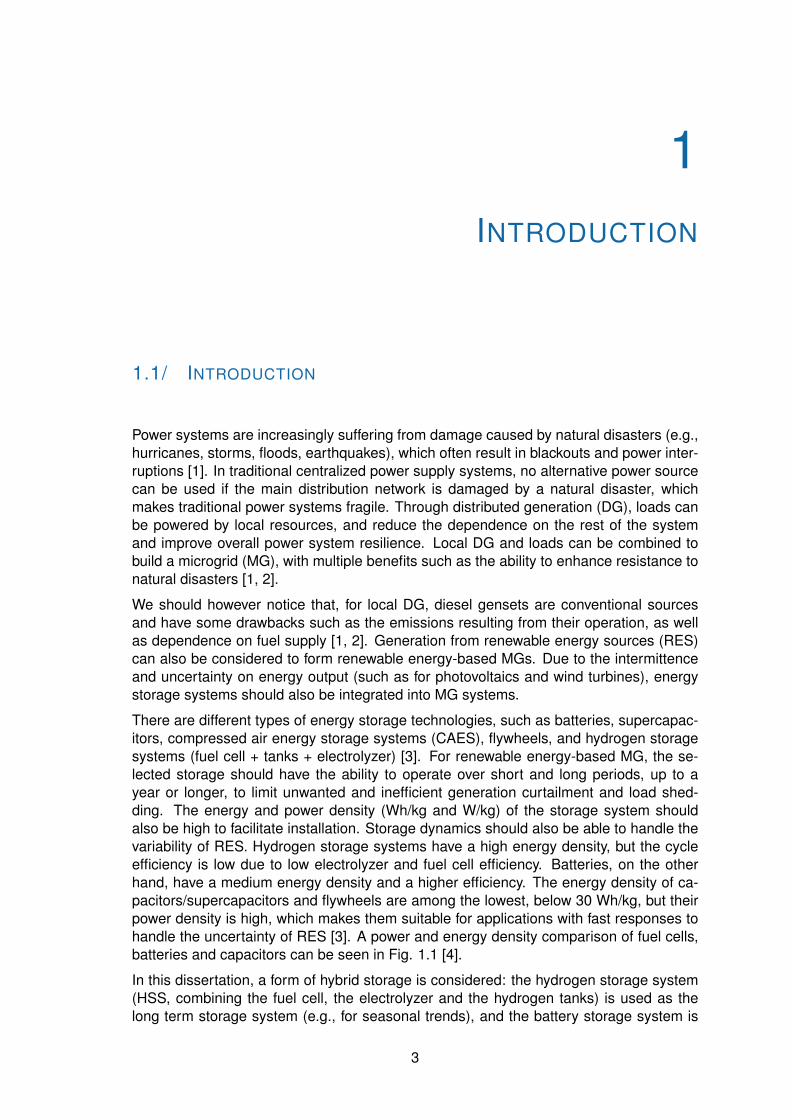
There are different types of energy storage technologies, such as batteries, supercapac-itors, compressed air energy storage systems (CAES), flywheels, and hydrogen storagesystems (fuel cell + tanks + electrolyzer) [3]. For renewable energy-based MG, the se-lected storage should have the ability to operate over short and long periods, up to ayear or longer, to limit unwanted and inefficient generation curtailment and load shed-ding. The energy and power density (Wh/kg and W/kg) of the storage system shouldalso be high to facilitate installation. Storage dynamics should also be able to handle thevariability of RES. Hydrogen storage systems have a high energy density, but the cycleefficiency is low due to low electrolyzer and fuel cell efficiency. Batteries, on the otherhand, have a medium energy density and a higher efficiency. The energy density of ca-pacitors/supercapacitors and flywheels are among the lowest, below 30 Wh/kg, but theirpower density is high, which makes them suitable for applications with fast responses tohandle the uncertainty of RES [3]. A power and energy density comparison of fuel cells,batteries and capacitors can be seen in Fig. 1.1 [4].
In this dissertation, a form of hybrid storage is considered: the hydrogen storage system(HSS, combining the fuel cell, the electrolyzer and the hydrogen tanks) is used as thelong term storage system (e.g., for seasonal trends), and the battery storage system is
3
4 CHAPTER 1. INTRODUCTION
Figure 1.1: Power and energy density comparison of fuel cell, battery and capacitor [4].
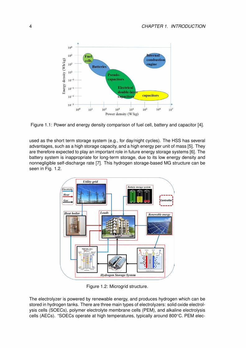
used as the short term storage system (e.g., for day/night cycles). The HSS has severaladvantages, such as a high storage capacity, and a high energy per unit of mass [5]. Theyare therefore expected to play an important role in future energy storage systems [6]. Thebattery system is inappropriate for long-term storage, due to its low energy density andnonnegligible self-discharge rate [7]. This hydrogen storage-based MG structure can beseen in Fig. 1.2.
Figure 1.2: Microgrid structure.
The electrolyzer is powered by renewable energy, and produces hydrogen which can bestored in hydrogen tanks. There are three main types of electrolyzers: solid oxide electrol-ysis cells (SOECs), polymer electrolyte membrane cells (PEM), and alkaline electrolysiscells (AECs). “SOECs operate at high temperatures, typically around 800oC. PEM elec-
1.1. INTRODUCTION 5
trolysis cells typically operate below 100oC and are becoming increasingly available com-mercially. AECs optimally operate at high concentrations of electrolyte (KOH or potassiumcarbonate) and at high temperatures, often near 200oC” [8]. A comparison of the differentelectrolyzer types can be found in [8, 9]. In this dissertation, an alkaline electrolyzer isused to convert the renewable energy output to hydrogen.
Hydrogen can then be supplied to a fuel cell to produce electricity and heat. There arefive main types of fuel cells: proton exchange membrane fuel cells (PEMFC), alkalinefuel cells (AFC), phosphoric acid fuel cells (PAFC), molten carbonate fuel cells (MCFC),and solid oxide fuel cells (SOFC). PEMFCs operate below 120oC, and use a proton-conducting polymer membrane containing the electrolyte solution that separates the an-ode and cathode sides [10]. AFCs, for which “the space between the two electrodesis filled with a concentrated solution of KOH or NaOH which serves as an electrolyte”,operate below 100oC [10]. PAFCs operate between 150oC and 200oC. “In these cellsphosphoric acid is used as a non-conductive electrolyte to pass positive hydrogen ionsfrom the anode to the cathode” [10]. MCFCs require a high operating temperature, typi-cally 650-700oC. “MCFCs use lithium potassium carbonate salt as an electrolyte, and thissalt liquefies at high temperatures, allowing for the movement of charge within the cell”[10]. Finally, SOFCs require high operating temperatures (800–1000oC) and can be runon a variety of fuels including natural gas. “SOFCs use a solid material, most commonlya ceramic material called yttria-stabilized zirconia (YSZ), as the electrolyte” [10]. A com-parison of different fuel cell can be found in [10, 11]. In this dissertation, a PEMFC isused to produce electricity and heat.
By enabling high penetration levels of RES, hydrogen-based MGs can be expected to playan important role in future smart grids, not only to friendly integrate RES (based on theenergy storage system to reduce the intermittence influence of renewable energy sourceson the utility grid and the demands), but also to resist to natural disasters (islanded op-eration ability under disasters). Moreover, integrating electricity supply with other formsof energy, such as gas or heat, can help further improve resilience as well as emissionsreduction.
In this thesis, we focus on the planning (sizing) and operation of hydrogen storage-based and multi-energy microgrids.
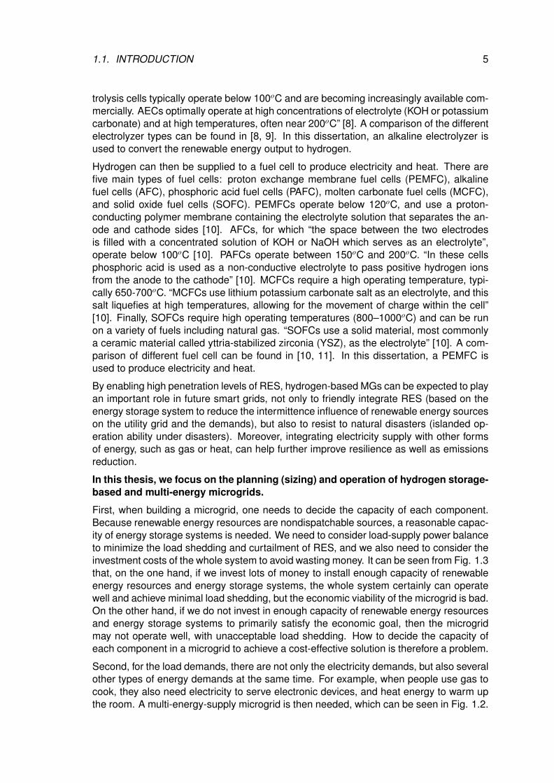
First, when building a microgrid, one needs to decide the capacity of each component.Because renewable energy resources are nondispatchable sources, a reasonable capac-ity of energy storage systems is needed. We need to consider load-supply power balanceto minimize the load shedding and curtailment of RES, and we also need to consider theinvestment costs of the whole system to avoid wasting money. It can be seen from Fig. 1.3that, on the one hand, if we invest lots of money to install enough capacity of renewableenergy resources and energy storage systems, the whole system certainly can operatewell and achieve minimal load shedding, but the economic viability of the microgrid is bad.On the other hand, if we do not invest in enough capacity of renewable energy resourcesand energy storage systems to primarily satisfy the economic goal, then the microgridmay not operate well, with unacceptable load shedding. How to decide the capacity ofeach component in a microgrid to achieve a cost-effective solution is therefore a problem.
Second, for the load demands, there are not only the electricity demands, but also severalother types of energy demands at the same time. For example, when people use gas tocook, they also need electricity to serve electronic devices, and heat energy to warm upthe room. A multi-energy-supply microgrid is then needed, which can be seen in Fig. 1.2.
6 CHAPTER 1. INTRODUCTION
Figure 1.3: Sizing values vs. Costs.
For such a microgrid, more components are needed, with for example, heating devicesto cover heat demands, and cooling devices to cover cooling demands. How to decidethe capacity of each component in the microgrid to achieve a cost-effective solution istherefore another, more complex problem. Additionally, for the energy storage system,long term running and frequent charging-discharging cause degradation over time. So,how the degradation of energy storage system will influence the sizing results is also aproblem.
Third, a multi-energy-supply microgrid can connect to the electricity/heat/gas utility grids.For this case, we need to consider the operation of the utility grid, because the microgridcan import energy from the utility grid, which will influence the energy flow of the wholesystem. So how to decide the capacity of each component in such a microgrid whenconsidering the utility grid is a also problem. In fact, for a large-node utility grid, the impactof contingency events (such as the destruction of the power lines) must be considered.When the utility grid is severely damaged under natural disasters, the islanded MG canstill operate to supply the load demands using the local renewable energy and the storagesystems. If the utility grid is partially destroyed, the MG power imports from the utility gridare limited, due to damage on transmission lines or pipelines. This means that the impactof contingency events will influence the MG power imports from the utility grid, and theninfluence the power flow inside the MG. At last, the sizing results of the components aredifferent.
Finally, when large amounts of multi-energy-supply microgrids are interconnected to theutility grid, how to operate this system well is another complex problem. Because of theprivacy concerns of each microgrid, centralized control (requiring to collect all informa-tion from all microgrids) is not practical. If the number of microgrids is in the hundreds,centralized control will also be impossible. So, how to operate a large numbers of multi-energy-supply microgrids interconnected with utility grid is a challenging problem.
1.2/ OBJECTIVES OF THE DISSERTATION
In this thesis, we therefore focus on microgrid sizing and operation problems. We explorethis problem from four perspectives:
1.3. OUTLINE OF THE DISSERTATION 7
1. Sizing of a full-electric hydrogen storage-based islanded microgrid.
2. Sizing of a multi-energy-supply islanded microgrid considering the degradation ofenergy storage systems.
3. Sizing of multi-energy-supply microgrids considering the gas/electricity/heat utilitygrid.
4. Sizing and price decision algorithm for multiple grid-connected multi-energy-supplymicrogrids.
In short, we first research about the sizing problem of a full-electric hydrogen-based islanded MG. Then, we expand the load demands to several types (electric-ity/heat/cooling/hydrogen), and research about the sizing problem of such a multi-energy-supply islanded microgrid. After that, we interconnect the microgrid into the utility grid,and research about the sizing problem of the grid-connected microgrid. Then, for thegrid-connected microgrid, the price must be considered, and we research about the pricedecision algorithm for multiple grid-connected multi-energy-supply microgrids. Also, thesizing algorithm for grid-connected MES MGs based on the different prices is presented.
Based on the above specific aspects, the detailed objectives of the dissertation can belisted as the following:
• Develop a strategy to control the operation of a microgrid.
• Develop a co-optimization-based sizing method.
• Present a rolling-horizon optimization method to check the sizing results.
• Integrate the degradation of energy storage systems in the sizing method.
• Consider the impact of contingency events on the sizing results of a micro-grid.
• Develop a price decision approach for multiple grid-connected microgrids.
• Develop a sizing algorithm for grid-connected MES MGs based on the differ-ent prices.
1.3/ OUTLINE OF THE DISSERTATION
The rest of this dissertation is structured as follows. Chapter 2 is contains a state-of-the-art review. The sizing and operation problem of hydrogen-based microgrids is introducedfrom four aspects: the model of the hydrogen-based microgrid, the operation strategy ofthe microgrid, the sizing method of the microgrid and the price decision algorithm for agrid-connected microgrid.
Chapter 3 presents the microgrid model. Two types of hydrogen-based microgrids aremodeled: the full-electric microgrid and the multi-energy supply microgrid.
Chapter 4 presents the sizing of a full-electric hydrogen storage system basedislanded microgrid. In this islanded microgrid, two storage systems are considered

8 CHAPTER 1. INTRODUCTION
(battery storage system and hydrogen storage system). A combined sizing and energymanagement methodology, formulated as a leader-follower problem, is presented. Theleader problem focuses on sizing and aims at selecting the optimal size for the microgridcomponents. It is solved using a genetic algorithm (GA). The follower problem, i.e., theenergy management issue, is formulated as a unit commitment problem and is solvedwith a mixed integer linear program (MILP). Uncertainties are considered using a formof robust optimization method. Several scenarios are modeled and compared in simula-tions to show the effectiveness of the proposed method, especially compared to a simplerule-based strategy.
Chapter 5 presents the sizing of a multi-energy-supply islanded microgrid consid-ering the degradation of energy storage system. A stand-alone microgrid consideringelectric power, cooling/heating and hydrogen consumption is built. A unit commitment al-gorithm, formulated as a MILP problem, is used to determine the best operation strategyfor the system. A GA is used to search for the best size of each component. The influenceof three factors (operation strategy, accuracy of load and renewable generation forecasts,and degradation of fuel cell, electrolyzer and battery) on sizing results is discussed. A1-h rolling horizon simulation is used to check the validity of the sizing results. A robustoptimization method is also used to handle the uncertainties and evaluate their impact onresults.
Chapter 6 presents the sizing of multi-energy-supply microgrids consideringgas/electric/heat utility grid. We focus on a gas/electricity/heat hybrid network. A hy-drogen storage system is used as the main electricity storage system. MILP is used todetermine the optimal operation of the multi-energy hybrid system, where the goal is tominimize shed load. A GA is used to search for the best size of each component, withthe goal to minimize the investment costs. In order to resist to contingency events, be-tweenness centrality (describing the relative importance of each node in a graph) is thenused to find the worst case under contingency events. This worst case scenario is usedto research about the influence of contingencies on the sizing results. At last, two cases(modified 13-node network and IEEE 30+Gas20+Heat14-nodes system) are tested usingthe proposed sizing method. The results show that the renewable energy location, in-vestment cost of components, and the structure of the whole system influence the sizingvalues of each component.
Chapter 7 presents the sizing and price decision algorithm for multiple grid-connected multi-energy-supply microgrids. Local generation, energy storage sys-tems, and renewable energy sources can form load service entities (LSE), which canprovide ancillary services to the utility grid and consumers. On the other hand, the mi-crogrids can also sell energy to load service entities/utility grid to obtain profits. But howthe load service entities can decide the selling electricity price to multiple microgrids, andhow the microgrids can decide the selling electricity price to load service entities are prob-lems. In this chapter, we present a guidance price decision method for multiple microgridsconsidering demand response. MILP is used to control the operation of each microgrid,and also used to operate the load service entities. GA is used to search for the best pricefor each microgrid and the load service entities. The simulation results show that thenew searched price works better than a time-of-use (TOU) price, which can reduce theoperation cost of the whole system. Also with higher penetration of renewable energy inMGs, the energy bought from the utility grid is reduced. At last, a large system is tested,in which 4 LSEs, 16 MGs and the IEEE 30-node network are considered. The simula-tion results show the feasibility of the presented pricing method. After then, in order to

1.3. OUTLINE OF THE DISSERTATION 9
reduce the GA searching time, a neural network (NN) model is presented to estimate theoperation of the whole system. Based on the NN model, the prices are obtained, andthe results show that the searching prices based on the NN model are better than withthe TOU price. After that, we present the sizing algorithm for grid-connected MES MGsbased on the different prices.
Finally, chapter 8 concludes on the thesis, by summarizing the main contributions andhighlighting possible future research areas.

2RELATED WORKS
In this chapter, related works about the sizing and operation problem of microgrids arereviewed. Three specific aspects are considered: 1) hydrogen-based microgrid; 2)
operation strategy of microgrid; 3) sizing method of microgrid. At last, when we considerthe grid-connected microgrid, the prices are often considered, then the related work aboutthe price decision approach in multiple multi-energy supply microgrids are reviewed.
2.1/ HYDROGEN-BASED MICROGRID
In order to limit global warming and reduce fossil fuel consumption, renewable energysources such as photovoltaic panels (PV) and wind turbines (WT) are more and morecommonly used to generate electricity. The integration of such intermittent sources isa challenge for grid operators, as the balance between generation and demand must bemet in real-time. This is especially a concern for small power systems such as microgrids,that can operate islanded, i.e., not connected to the main grid. Microgrids typically includedistributed generation and storage [12, 13], and are increasingly found in remote areas[14, 15] or where power system resilience is a crucial concern [1, 16].
To enable RES integration, energy storage systems are considered as a key solution,as they enable storing excess generation for later use [17]. Battery storage systems(BSS) are typically used for short-term storage [18], but seem inappropriate for long-termstorage [7]. Hydrogen storage systems (HSS) have a high energy density [3], and areused for long-term storage, such as seasonal storage. HSSs combine an electrolyzer toproduce hydrogen from electricity, a hydrogen storage tank and a fuel cell (FC) to produceelectricity from hydrogen.
Works about hydrogen-based full-electric microgrid have been presented in the liter-ature. For example, [19] discusses FC systems, while [20] researches about the controlstrategy of PV/FC hybrid systems. In [21], a Matlab/Simulink model is built to simulatea grid-connected PV/FC hybrid system. [22] also builds a simulation model of anotherPV/FC/ultacapacitors stand-alone microgrid.
On the other hand, when there are different types of load demands, such as electricity,heat, cooling or hydrogen, “combined cooling heat and power systems” are typically usedto form multi-energy-supply microgrids. Different devices can be chosen to build a multi-energy-supply microgrid. The main component is the prime mover (the combined heatand power plant). For a traditional system, there are several types of prime movers, suchas internal combustion engine, combustion turbine, steam turbine, micro-turbine, stirling
11
12 CHAPTER 2. RELATED WORKS
engine, etc. A comparison of these prime movers can be seen in [23].
Fuel cells are a promising technology for efficient and sustainable energy conversion[24], and are expected to play an important role in future distributed energy generation[6]. Xe adopt the fuel cell as the equivalent of a “prime mover” that produces electricityand heat. The fuel cell consumes hydrogen, which is emissions-free when it is generatedfrom renewable energy and water electrolysis.
Thus, a hydrogen-based multi-energy-supply microgrid can be built. Some worksabout fuel cell based multi-energy-supply microgrid have been presented. For example,[25] investigates the feasibility of combining an SOFC and a gas turbine system for marineapplications. The efficiency of the configuration with double-effect absorption chiller canachieve 43.2% compared to 12% for the conventional system. In [26], an SOFC witha capacity of 215 kW is combined with a recovery cycle and is used to meet the loaddemand in a hotel. The results show that based on fuel lower heating value, a maximumefficiency of 83% for simultaneous energy generation and heat recovery cycle can beachieved.
According to industry analysts Delta-ee, fuel cell CHP units represent 64% of the CHPunit sale market, which doubles the results from 2011. It is becoming the most commontechnology employed in micro-CHP systems [23].
The above papers show that hydrogen-based microgrids are expected to play an impor-tant role in future smart grids. The structure of such hydrogen-based microgrid can beseen in Fig.1.2. In the following section, the operation strategy of hydrogen-based micro-grids is introduced.
2.2/ OPERATION STRATEGY OF MICROGRID
The operation strategy of an MG system needs to be considered from two aspects: timescale and solution method.
Based on the selected time scale, two strategies can be considered: day-ahead schedul-ing and short term dispatching. A day-ahead scheduler provides unit commitment solu-tions aiming to find cost-effective combinations of generating units output, while a shortterm dispatcher returns the economic dispatch aiming to minimize the operation cost ofthe committed assets based on short term forecasts.
In [27], authors review the energy management of a microgrid, and point out that basedon the time scale, two scheduling strategies (unit commitment and economic dispatch)are used together. In [28], a multi-timescale MG scheduling and dispatching strategy isdeveloped for the coupled multi-type energy supply in an MG. In day-ahead scheduling,the objective function is to minimize the operation cost, and the objective of real-timedispatching is to make the real-time actual electricity power exchange between the MGand to make the main grid follow its day-ahead schedules as close as possible. In [29],authors present a two-stage coordinated control approach for CCHP microgrid energymanagement. The first stage is a rolling-horizon economic dispatch. The second stageis a real-time adjustment stage, which adjusts the controllable sources to make the real-time energy exchanged with the main grid and the state of the battery follow its economicdispatch as closely as possible.
In our sizing problem, our goal is to decide the sizing value of each component in the MG
2.2. OPERATION STRATEGY OF MICROGRID 13
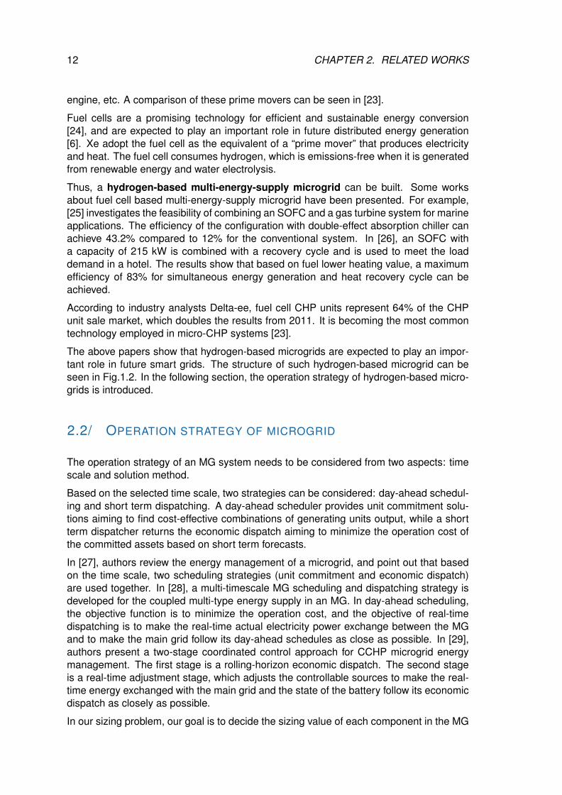
system. So we not only need to consider the long-term planning (e.g. one year), namelyto make the MG system cost-effective, but we also need to consider the short-term oper-ation (e.g. 1 hour) to make the MG system operate normally, as illustrated in Fig. 2.1. Ifthe selected time scale is small (such as 1 minute), the short-term operation will be moreprecise, but the long-term planning will cause lots of computation burden. On the otherhand, if the selected time scale is large (such as 1 day), the short-term operation checkwill be not precise, but the long-term planning will cause a small computation burden.This relationship can be seen in Fig. 2.2.
Figure 2.1: Sizing and operation.
Figure 2.2: Computation burden, operation error vs. time scale.
Based on the above analysis, considering the tradeoff between accuracy and the compu-tation burden, hourly profiles are adopted in the operation strategy [30].
In the following subsections, we mainly introduce the solution method of the operationproblem. We classify this from two specific aspects: 1) the operation of full-electric mi-crogrid; 2) the operation of multi-energy supply microgrid.
2.2.1/ OPERATION OF FULL-ELECTRIC MICROGRID
In this section, we review related works about the operation problem of full-electric micro-grids.
A simple operation strategy is often selected to operate the full-electric microgrid, namely,the load following (LF) strategy: when there is surplus power, the excess energy is storedin the ESS, and when there is a shortage of power, the ESS discharges, or controllablegenerators (diesel gensets or FC) are turned on. Economic criteria are not considered inmost cases.
14 CHAPTER 2. RELATED WORKS
For example, [31, 32] compare several EA for the optimal sizing of a hybrid MG system,where the objective function is the total annual cost, and the operation strategy is theLF strategy. Other papers use various metaheuristics to search for the sizing values fordifferent MG cases, and the operation principle is also LF. [33] uses ant colony optimiza-tion (ACO) to determine the size values of a PV/wind hybrid system, where the objectivefuntion is the sum of the total capital cost and total maintenance cost. In [34], artificialbee swarm optimization (ABSO) is used to solve the sizing problem of PV/WT/FC hybridsystem considering the loss of power supply probability (LPSP). [35] studies the perfor-mance of different particle swarm optimization (PSO) algorithm variants to determine thesize results of a hybrid (PV/wind/Batt) system.
Some papers use more advanced strategies based on rules (rule-based strategies (RBS))to control energy flows. For example, in [36], the operation mode of the islanded MG isdetermined by the SOC of the battery storage. Three operation modes are set basedon different rules to achieve the goals, such as maximize the utilization of the RES units,or ensure the reliability and longevity of the battery storage. In [37], the energy flow iscontrolled depending on the charge and discharge states, different rules are built basedon the preset parameters. In [38], authors set knowledge-based rules to control theoperation of a diesel generator for an isolated MG with diesel-wind-ESS resources. Theobjective of this rule-based strategy is to minimize the diesel generation by minimizingthe power wasted through the dump load for every hour.
The main advantage of using an RBS is that it can optimize the system performance with-out requiring an optimization function or tools, thus reducing computational complexity[38]. However, the limits of RBS are quickly reached when more than a few componentsare included in the system, as the number of required rules significantly increases. More-over, these strategies cannot provide optimal results regarding how the state-of-chargeof storage units is controlled over time.
More advanced energy management systems (EMS) that primarily focus on economicdispatch with EA, are also presented in the literature. [39] proposes a bilevel optimizationenergy management approach of multiple microgrids. Economic dispatch is solved ineach microgrid, and then a secondary-level optimization is used to seek the minimumoperation cost for the set of microgrids. Multiperiod ABCO [40], multi-layer ACO [41] arealso used for economic dispatch applications. The objective of the economic dispatchproblem is to minimize the total production cost while satisfying generation resourcesconstraints.
EA-based optimization relies on stochastic search, which can give a satisfatory solutionwith a reasonable computation time, but it does not guarantee obtaining an optimal solu-tion.
An improved method for energy management that can take into account multiple objec-tives and constraints is thus required. Model-predictive control (MPC) offers a solution,and is commonly used in power systems in the form of unit commitment (UC). UC en-ables scheduling the use of multiple generation units over a given time horizon [42], forexample over a day. It can also be extended to consider storage units and other devices.For example, in [7], authors present a UC optimization method to economically scheduleBSS and HSS. [43] studies the thermal power plant UC problem integrated with a largescale ESS. In [44], an integrated framework for a stand-alone microgrid with objectivesof increasing stability and reliability and reducing costs is described. The UC method isused to determine generators outputs for the next day. [45] presents a two-stage planning
2.2. OPERATION STRATEGY OF MICROGRID 15
and design method for microgrids. GA is used to solve the optimal design problem and aMILP algorithm enables determining the optimal operation strategy.In [46], a mixed inte-ger nonlinear programming (MINLP) approach for day-ahead scheduling of a combinedheat and power plant is proposed. Another MINLP-based EMS algorithm is presentedin [47]. [48] describes an approach for security-constrained UC with integrated ESS andwind turbines.
Overall, the above research papers show that the UC method is commonly used andadequate for scheduling the use of microgrid components, including energy storage units.The advantage and disadvantage of UC optimization-based EMS can be concluded asfollows:
• Advantages:
1. compared to EA algorithms, UC optimization can simply consider varieties ofconstraints, e.g., binary variable constraints (ON/OFF state of battery, etc.),continuous variable constraints (ouput power of fuel cell, etc.), logical con-straints (charging and discharging can not occur at the same time, etc.), andso on;
2. compared to RBS strategy, UC optimization can simply set the operation pri-ority of each component by adjusting parameters in the objective function, andcan also consider the economic criteria and different constraints as in 1).
• Disadvantages:
1. require an optimization function or tools;
2. the computation complexity and time burden is increasing as the number ofvariables increases;
3. especially, when there are nonlinear constraints or variables, the UC problemcauses lots of computation burden.
A UC algorithm does however rely on forecast data to compute schedules. As forecastingerrors are inevitable, the scheduling algorithm must consider these errors. In the casestudied in this paper, errors on PV output and load impact schedules as well as sizingresults. Two main approaches to consider forcasting uncertainty are found in the litera-ture: the scenario-based method [49, 50, 51] and robust optimization [52, 53, 54, 55]. [49]presents a stochastic method based on cloud theory to handle uncertainty, and uses a krillherd algorithm to solve the optimization problem. [50] describes a stochastic optimizationfor microgrid energy and reserve scheduling. Wind and PV generation fluctuations foreach hour are represented by 5 interval discrete probability distribution functions. A sce-nario tree technique is then used to combine different states of wind and PV fluctuations.[51] presents a scenario-based robust energy management method. Taguchi’s orthogo-nal array testing method is used to provide possible testing scenarios, and determine theworst-case scenario. At last, the Monte Carlo method is used to verify the robustnessof the approach. In [52], uncertainty is quantified in terms of prediction intervals by anon-dominated sorting genetic algorithm (NSGA-II) trained by a neural network. Robustoptimization is then used to seek the optimal solution to the problem. [53] uses robustoptimization-based scheduling for multiple microgrids considering uncertainty. The prob-lem is transformed into a min-max robust problem, and is then solved using linear dualitytheory and the Karush-Kuhn-Tucker (KKT) optimality conditions. [55] presents a robust
16 CHAPTER 2. RELATED WORKS
EMS for microgrids. Authors use a fuzzy prediction interval model to obtain the uncer-tainty boundary of wind output, and then the upper and lower boundaries of wind energyare interpreted as the best and worst-case operating conditions.
In the above papers, scenario-based methods usually require generating many scenarios,which can take a lot of time to simulate. On the other hand, robust methods are usedto find the worst case, which requires less computation time although results are moreconservative. As a consequence, in this thesis, a robust optimization method is selectedto find the worst case and best case based on the forecasting error.
In this section, different operation strategies are presented for full-electric MG, includ-ing LF-EMS, RBS-EMS, EA-EMS, and UC-EMS. In the following section, the operationstrategy for CCHP MG is presented.
2.2.2/ OPERATION OF MULTI-ENERGY SUPPLY MICROGRID
Regarding the solution method (i.e., decision-making), the operation strategies of a CCHPsystem can be also divided into two main types: rule-based strategies and optimization-based strategies.
In a multi-energy system, several loads must be satisfied. This means that some priorityrules must be set, leading to traditional rule-based strategies: following the electric load(FEL), following the thermal load (FTL) or following the cooling load (FCL). In [56], authorsreview different optimization operation strategies, including basic operation strategies andhybrid operation strategies. [57] presents a novel optimal operational strategy for a CCHPsystem based on two typical operating modes: FEL and FTL. An integrated performancecriterion which considers primary energy consumption, carbon dioxide emissions andoperational cost, is used to decide which operating mode is chosen. In [58], authorscompare five strategies: electrical-equivalent load following, continuous operation, peakshaving, and base load. In [59], five operation strategies are compared: FCL, FTL, FEL,maximum power output, and waste heat allocation proportion. [60] presents a multi-agent-based demand-side energy management system for autonomous polygenerationmicrogrids. With three types of demands (electricity, hydrogen, potable water). The goalsare to have no potable water and hydrogen shortages, and to prevent the battery fromdeep discharging. The activation of each agent is based on rules. These rule-based op-eration strategies are however difficult to use for complex systems, where a large numberof rules are needed, especially in multiple energy system.
Due to the drawbacks of rule-based strategies, optimization methods are also commonlyused. A first category includes heuristic optimization methods, which are adequate tosolve non-linear and non-convex problems. [61] proposes a time-varying accelerationcoefficient particle swarm optimization (PSO) algorithm to solve the non-linear and non-convex CHP economic dispatch problem. The objective is to minimize the total heat andpower production cost. [62] presents an artificial immune system algorithm for solving theCHP economic dispatch problem. The objective is to minimize the total fuel cost. [63]proposes a bacterial foraging-based fuzzy satisfactory optimization algorithm to solvethe multi-objective energy management problem for a CHP-based microgrid. The ob-jectives are to minimize the total operating cost and the emissions. [64] introduces amulti-objective PSO economic dispatch optimization method for a system that incorpo-rates CHP and wind power units. [65] proposes a multi-objective optimization modelwhich aims to maximize the energy-saving ratio and minimize the energy costs of a micro-
2.3. SIZING METHOD OF MICROGRID 17
CCHP system. [66] presents a scenario-based scheduling method for a fuel cell-basedCHP microgrid, which aims at maximizing the expected profit. A modified firefly algorithmis used to solve the problem.
As discussed in section 2.2.1, “EA-based optimization relies on stochastic search, whichcan give a satisfatory solution with a reasonable computation time, but it does not guar-antee obtaining an optimal solution”.
The second category corresponds to mixed integer programming optimization (MIP),which uses deterministic methods. [67] explores opportunities for increasing the flexi-bility of CHP units using electrical boilers and heat storage tanks for better integration ofwind power. A linear model is proposed for the centralized dispatch of integrated energysystems. [68] presents an MILP optimization model for combined cooling, heat and powersystem operation. The objective is to minimize the total operation and maintenance costs.[69] presents the optimization of a CCHP system using MILP to determine the preliminarydesign of such systems with thermal storage. The objective function is to minimize thetotal annual cost. The effect of legal constraints in the design and operation of CCHPsystems is highlighted in this study. In [70], the objective of the operation strategy is tomaximize the gross operational margin and net present value, and the problem is formu-lated as an MIP model. In [71], the optimal control problem is formulated as an MINLP,and is solved using discrete dynamic programming. In [45], an MILP algorithm is used tosolve the optimal dispatch problem, and the objective function is to minimize the operationcost. In [72], an operation strategy is formulated as an MILP problem aiming to maximizegreenhouse gas emissions reductions.
UC optimization, formulated as an MILP problem, can be solved using a linear-programming based branch-and-bound algorithm [73], which is appropriate to solve en-ergy management problems in CCHP systems. The optimal sheduling set points aredetermined based on current and future conditions, which can guarantee obtaining theglobal optimal results.
In a CCHP system, a rule-based operation strategy is difficult to use, because a largenumber of rules would need to be built to satisfy the power flow and system constraints.In EA operation strategies, premature convergence and reasonable computation timesneed to be considered. In this thesis, we adopt the UC method to control the operation ofthe CCHP microgrid system. The optimization problem is formulated as an MILP problem,and several constraints are used to describe different operation strategies.
2.3/ SIZING METHOD OF MICROGRID
The above section 2.2 introduced the operation strategy for different types of MGs. Asshown in Fig. 2.1, after we know the operation strategy of the MGs, then we canfind a method to size the MGs. For the sizing problem, the goal is to achieve cost-effectiveness, namely, minimize the total costs (including investment, maintenance, op-eration and penalty costs) of the system, and at same time, satisfy different constraints(e.g. technical criteria, logical constraints etc.).
In this section, sizing methods of microgrids are introduced. We also introduce this prob-lem from three aspects:
1. the sizing of a full-electric microgrid;
18 CHAPTER 2. RELATED WORKS
2. sizing of a multi-energy supply microgrid;
3. sizing of a multi-energy supply microgrid considering utility grids.
2.3.1/ SIZING OF FULL-ELECTRIC MICROGRID
The optimal sizing problem is a non-convex and non-linear combinatorial optimizationproblem [32], and for the solution of this problem, various optimization methods havebeen presented in [74].
Firstly, there are large numbers of simulation tools to solve the combination sizing prob-lem. In [75], authors review 68 computer tools which can be used for analyzing RESintegration, but the results show that there is no tool that can address all aspects of hy-brid microgrid systems.
The conventional method is the trial-and-error method: firstly, list all combinations of thesizing values; after that, deploy these combinations in the simulation model to calculatethe annual total cost of the system; at last, the solution with the lowest annual total costcontains the optimum sizing values. This method will be impossible to deploy, becausethe combination of sizing values will be large when there are several sizing variables,which leads to lots of computation time.
At last, the most appropriate method to solve the combination sizing problem is the evo-lutionary algorithm (EA) [32, 74].
For example, [31, 32] compare several EAs for the optimal sizing of a hybrid system,where the objective function is the total annual cost. Other papers use various meta-heuristics, such as [33] which uses ACO to get size values of a PV/wind hybrid system.In [34], ABSO is used to solve the sizing problem of a PV/WT/FC hybrid system consider-ing loss of power supply probability. Simulated annealing and tabu search (TS) are usedin [14]. [35] studies the performance of different PSO algorithm variants to determine thesize results of a hybrid (PV/wind/battery) system.
In section 2.2.1, the operation strategy of the full-electric MG has been presented. Thenwith the EA method, the sizing problem considering energy management of a full-electricMG can be solved. This co-optimization algorithm considering the combinations of sizingand energy management is shown in Fig. 2.1.
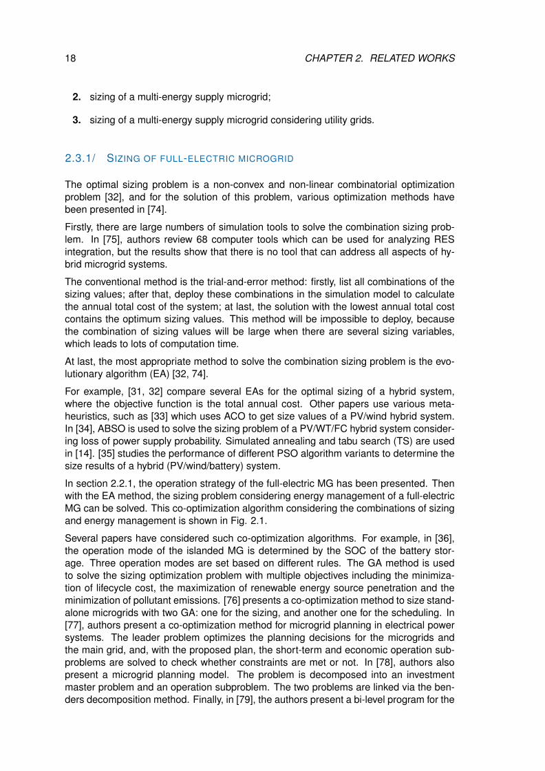
Several papers have considered such co-optimization algorithms. For example, in [36],the operation mode of the islanded MG is determined by the SOC of the battery stor-age. Three operation modes are set based on different rules. The GA method is usedto solve the sizing optimization problem with multiple objectives including the minimiza-tion of lifecycle cost, the maximization of renewable energy source penetration and theminimization of pollutant emissions. [76] presents a co-optimization method to size stand-alone microgrids with two GA: one for the sizing, and another one for the scheduling. In[77], authors present a co-optimization method for microgrid planning in electrical powersystems. The leader problem optimizes the planning decisions for the microgrids andthe main grid, and, with the proposed plan, the short-term and economic operation sub-problems are solved to check whether constraints are met or not. In [78], authors alsopresent a microgrid planning model. The problem is decomposed into an investmentmaster problem and an operation subproblem. The two problems are linked via the ben-ders decomposition method. Finally, in [79], the authors present a bi-level program for the
2.3. SIZING METHOD OF MICROGRID 19
sizing of islanded microgrids with an integrated compressed air energy storage (CAES).The upper level problem is solved using GA, and the lower level problem is solved usingthe MILP technique.
2.3.2/ SIZING OF MULTI-ENERGY SUPPLY MICROGRID
The above section presented the sizing method of the full-electric MG, and the co-optimization method is often adopted. In this section, the sizing method of multi-energysupply MG is presented.
The traditional sizing method for CCHP systems is the maximum rectangle method(MRM) which uses the hourly load curve and finds the rectangle area under this curve[80], [81]. But this method cannot represent the dynamic, changing performance of thesystem.
Co-optimization methods are also adopted to search for the optimal sizing values inCCHP MGs. Based on different sizing methods and different operation strategies, theco-optimization methods can be classified as the following types:
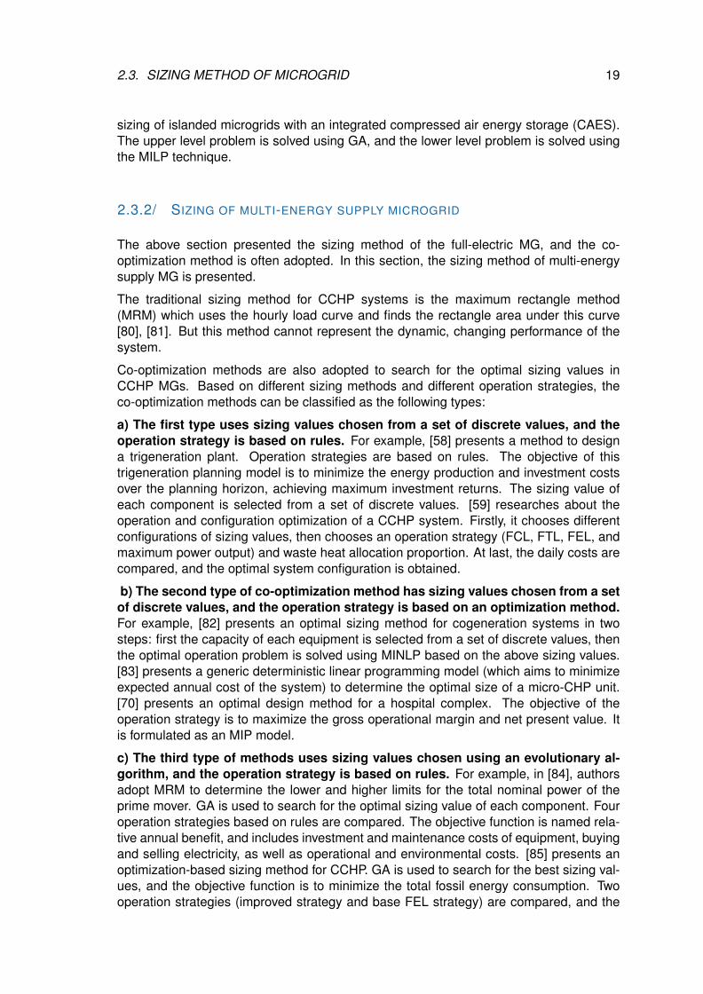
a) The first type uses sizing values chosen from a set of discrete values, and theoperation strategy is based on rules. For example, [58] presents a method to designa trigeneration plant. Operation strategies are based on rules. The objective of thistrigeneration planning model is to minimize the energy production and investment costsover the planning horizon, achieving maximum investment returns. The sizing value ofeach component is selected from a set of discrete values. [59] researches about theoperation and configuration optimization of a CCHP system. Firstly, it chooses differentconfigurations of sizing values, then chooses an operation strategy (FCL, FTL, FEL, andmaximum power output) and waste heat allocation proportion. At last, the daily costs arecompared, and the optimal system configuration is obtained.
b) The second type of co-optimization method has sizing values chosen from a setof discrete values, and the operation strategy is based on an optimization method.For example, [82] presents an optimal sizing method for cogeneration systems in twosteps: first the capacity of each equipment is selected from a set of discrete values, thenthe optimal operation problem is solved using MINLP based on the above sizing values.[83] presents a generic deterministic linear programming model (which aims to minimizeexpected annual cost of the system) to determine the optimal size of a micro-CHP unit.[70] presents an optimal design method for a hospital complex. The objective of theoperation strategy is to maximize the gross operational margin and net present value. Itis formulated as an MIP model.
c) The third type of methods uses sizing values chosen using an evolutionary al-gorithm, and the operation strategy is based on rules. For example, in [84], authorsadopt MRM to determine the lower and higher limits for the total nominal power of theprime mover. GA is used to search for the optimal sizing value of each component. Fouroperation strategies based on rules are compared. The objective function is named rela-tive annual benefit, and includes investment and maintenance costs of equipment, buyingand selling electricity, as well as operational and environmental costs. [85] presents anoptimization-based sizing method for CCHP. GA is used to search for the best sizing val-ues, and the objective function is to minimize the total fossil energy consumption. Twooperation strategies (improved strategy and base FEL strategy) are compared, and the
20 CHAPTER 2. RELATED WORKS
primary energy saving ratio is employed to evaluate the strategy. [86] describes a thermo-dynamic performance analysis to optimize the configurations of a hybrid CCHP systemincorporating solar energy and natural gas. GA is used to search for the best configura-tion, and the operation strategy is based on rules. The objective function is to maximizethe annual primary energy savings and the annual total cost savings.
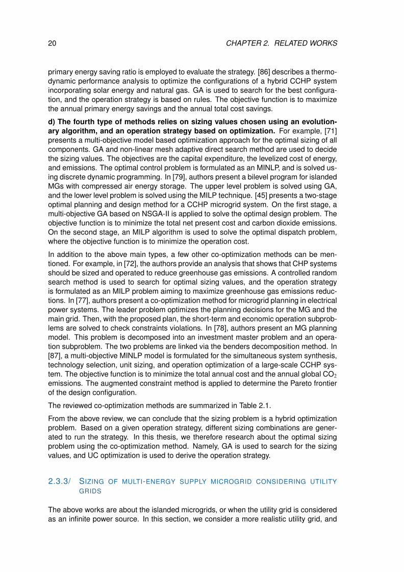
d) The fourth type of methods relies on sizing values chosen using an evolution-ary algorithm, and an operation strategy based on optimization. For example, [71]presents a multi-objective model based optimization approach for the optimal sizing of allcomponents. GA and non-linear mesh adaptive direct search method are used to decidethe sizing values. The objectives are the capital expenditure, the levelized cost of energy,and emissions. The optimal control problem is formulated as an MINLP, and is solved us-ing discrete dynamic programming. In [79], authors present a bilevel program for islandedMGs with compressed air energy storage. The upper level problem is solved using GA,and the lower level problem is solved using the MILP technique. [45] presents a two-stageoptimal planning and design method for a CCHP microgrid system. On the first stage, amulti-objective GA based on NSGA-II is applied to solve the optimal design problem. Theobjective function is to minimize the total net present cost and carbon dioxide emissions.On the second stage, an MILP algorithm is used to solve the optimal dispatch problem,where the objective function is to minimize the operation cost.
In addition to the above main types, a few other co-optimization methods can be men-tioned. For example, in [72], the authors provide an analysis that shows that CHP systemsshould be sized and operated to reduce greenhouse gas emissions. A controlled randomsearch method is used to search for optimal sizing values, and the operation strategyis formulated as an MILP problem aiming to maximize greenhouse gas emissions reduc-tions. In [77], authors present a co-optimization method for microgrid planning in electricalpower systems. The leader problem optimizes the planning decisions for the MG and themain grid. Then, with the proposed plan, the short-term and economic operation subprob-lems are solved to check constraints violations. In [78], authors present an MG planningmodel. This problem is decomposed into an investment master problem and an opera-tion subproblem. The two problems are linked via the benders decomposition method. In[87], a multi-objective MINLP model is formulated for the simultaneous system synthesis,technology selection, unit sizing, and operation optimization of a large-scale CCHP sys-tem. The objective function is to minimize the total annual cost and the annual global CO2emissions. The augmented constraint method is applied to determine the Pareto frontierof the design configuration.
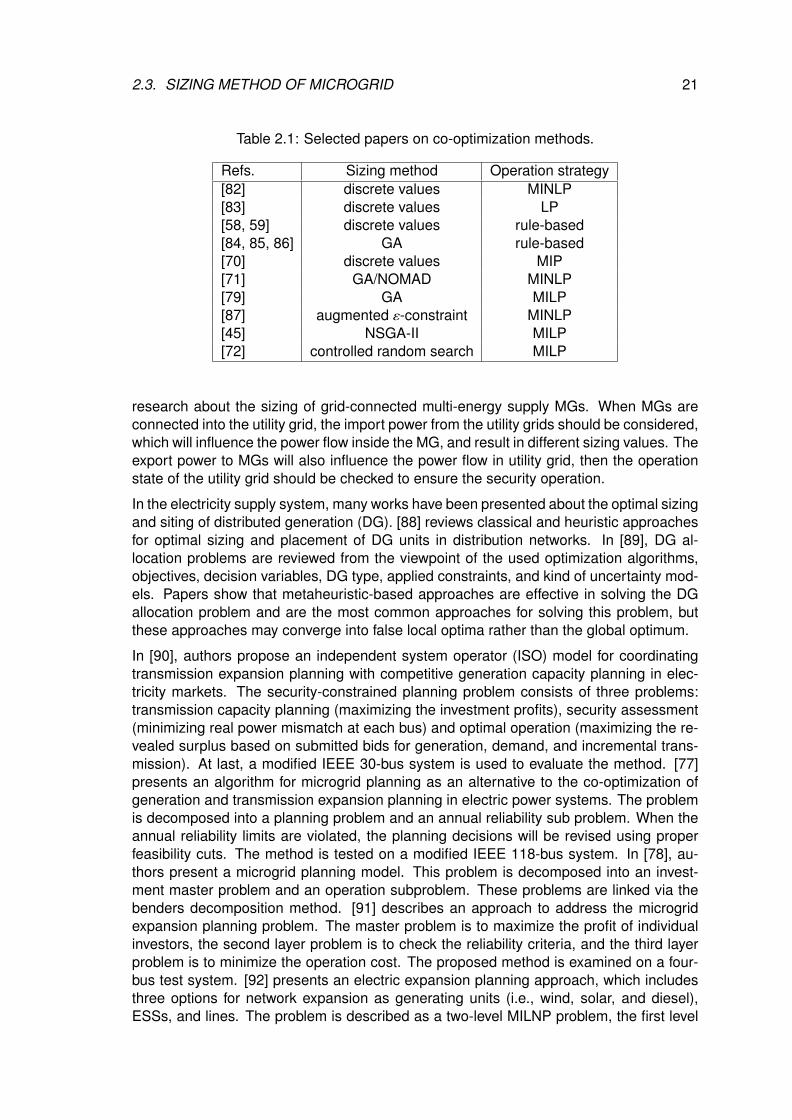
The reviewed co-optimization methods are summarized in Table 2.1.
From the above review, we can conclude that the sizing problem is a hybrid optimizationproblem. Based on a given operation strategy, different sizing combinations are gener-ated to run the strategy. In this thesis, we therefore research about the optimal sizingproblem using the co-optimization method. Namely, GA is used to search for the sizingvalues, and UC optimization is used to derive the operation strategy.
2.3.3/ SIZING OF MULTI-ENERGY SUPPLY MICROGRID CONSIDERING UTILITYGRIDS
The above works are about the islanded microgrids, or when the utility grid is consideredas an infinite power source. In this section, we consider a more realistic utility grid, and
2.3. SIZING METHOD OF MICROGRID 21
Table 2.1: Selected papers on co-optimization methods.
Refs. Sizing method Operation strategy[82] discrete values MINLP[83] discrete values LP[58, 59] discrete values rule-based[84, 85, 86] GA rule-based[70] discrete values MIP[71] GA/NOMAD MINLP[79] GA MILP[87] augmented ε-constraint MINLP[45] NSGA-II MILP[72] controlled random search MILP
research about the sizing of grid-connected multi-energy supply MGs. When MGs areconnected into the utility grid, the import power from the utility grids should be considered,which will influence the power flow inside the MG, and result in different sizing values. Theexport power to MGs will also influence the power flow in utility grid, then the operationstate of the utility grid should be checked to ensure the security operation.
In the electricity supply system, many works have been presented about the optimal sizingand siting of distributed generation (DG). [88] reviews classical and heuristic approachesfor optimal sizing and placement of DG units in distribution networks. In [89], DG al-location problems are reviewed from the viewpoint of the used optimization algorithms,objectives, decision variables, DG type, applied constraints, and kind of uncertainty mod-els. Papers show that metaheuristic-based approaches are effective in solving the DGallocation problem and are the most common approaches for solving this problem, butthese approaches may converge into false local optima rather than the global optimum.
In [90], authors propose an independent system operator (ISO) model for coordinatingtransmission expansion planning with competitive generation capacity planning in elec-tricity markets. The security-constrained planning problem consists of three problems:transmission capacity planning (maximizing the investment profits), security assessment(minimizing real power mismatch at each bus) and optimal operation (maximizing the re-vealed surplus based on submitted bids for generation, demand, and incremental trans-mission). At last, a modified IEEE 30-bus system is used to evaluate the method. [77]presents an algorithm for microgrid planning as an alternative to the co-optimization ofgeneration and transmission expansion planning in electric power systems. The problemis decomposed into a planning problem and an annual reliability sub problem. When theannual reliability limits are violated, the planning decisions will be revised using properfeasibility cuts. The method is tested on a modified IEEE 118-bus system. In [78], au-thors present a microgrid planning model. This problem is decomposed into an invest-ment master problem and an operation subproblem. These problems are linked via thebenders decomposition method. [91] describes an approach to address the microgridexpansion planning problem. The master problem is to maximize the profit of individualinvestors, the second layer problem is to check the reliability criteria, and the third layerproblem is to minimize the operation cost. The proposed method is examined on a four-bus test system. [92] presents an electric expansion planning approach, which includesthree options for network expansion as generating units (i.e., wind, solar, and diesel),ESSs, and lines. The problem is described as a two-level MILNP problem, the first level
22 CHAPTER 2. RELATED WORKS
is to minimize the planning cost, and the second level is to minimize the operation cost.Both problems are solved by a hybrid meta-heuristic optimization technique which collectsthe benefits of particle swarm optimization (PSO), cultural algorithm, and co-evolutionaryalgorithms at the same time.
The above papers use the co-optimization methods to solve the microgrid planning prob-lem. The co-optimization method decomposes the planning problem into a master prob-lem and a subproblem which can consider two time scales: long term planning and shortterm operation. The master problem aims to search for the planning results, and thesubproblem is to evaluate the correctness of the operation problem.
Some works about the sizing problem of multi-energy microgrids have also been pub-lished, as shown in section 2.3.2. Also the sizing problem of multi-energy microgridsconsidering utility grid are presented. For example, in [93], authors present an MILPmodel for the optimal design of DG systems coupled with heating, cooling, and powerdistribution networks, aiming to minimize the annual overall cost. [94] presents a multi-objective optimization approach based on GA for CHP system within microgrid system.The two objectives are to minimize the total cost and the total gas emissions from themain grid, boiler and DG units. The operation strategies are “following electrical load”and “following thermal load”.
Works about the co-planning of natural gas and power electric systems are also re-searched. For example, in [95], an integrated electricity and natural gas transportationsystem planning algorithm is proposed for enhancing the power grid resilience in extremeconditions. The first stage problem is to minimize the investment and the operation costsfor the integrated electricity and natural gas, the second stage problem is to minimize loadcurtailment after the occurrence of the most severe event. The test results on the IEEE-RTS1979 point out that the integrated planning of electricity and natural gas can improvethe power system resilience. [96] proposes a long-term co-optimization planning modelwhich incorporates the natural gas infrastructure planning in power system planning. Theinvestment problem is formulated to optimally determine appropriate candidates for gen-erating units, transmission lines, and natural gas pipelines. The second subproblem isthe power system feasibility and optimality (minimizing the load curtailment). The thirdsubproblem is the natural gas transportation feasibility (minimizing the nodal natural gasload imbalance). At last, the power system reliability is evaluated. [97] proposes an in-tegrated expansion planning framework for gas and power systems. The model aimsto maximize the benefit/cost ratio by calculating benefits in operation reduction, carbonemissions reduction and reliability improvement against augmentation investment costs.[98] presents a long-term, multiarea, and multistage model for supply/interconnectionsexpansion planning of an integrated electricity and natural gas system. The proposedmodel is formulated as an optimization problem, which minimizes the investment and op-eration costs to determine the optimal location, technologies, and installation times of anynew facility for power generation, power interconnections, and the complete natural gaschain value (supply/transmission/storage) as well as the optimal dispatch of existing andnew facilities over a long range planning horizon.
The co-planning method can consider the characteristics of the power system and thenatural gas system at the same time, which includes the interactions between both sys-tems on supply and demand sides, and help achieve higher market efficiency in the costbenefit analysis [97].
However research works about the sizing problem of gas/electricity/heat hybrid systems
2.4. PRICE DECISION ALGORITHM FOR GRID-CONNECTED MICROGRIDS 23
have not been given a lot of attention so far. [30] researched about the sizing problem ofan electricity/heat system, and showed that a single-node aggregate approach (namely,ignore the interconnection structure inside the microgrid) cannot capture the internal en-ergy transfers and the limitations of the electrical/thermal networks.
2.4/ PRICE DECISION ALGORITHM FOR GRID-CONNECTED MICRO-GRIDS
When the MGs are connected into the utility grid, the prices must be considered. MGscan buy energy from the utility grid, and also can sell energy to utility grid. So how todecide the selling prices of utility grid, and selling prices of MGs are essential problems.
Then in this section, we review related works about the price decision method for MGs.The price decision approaches can be classified into two main categories: 1) game theoryapproaches; 2) bilevel approaches.
2.4.1/ GAME THEORY APPROACH
In this subsection, we introduce price decision using the game theory approach. Onefunction of the price is to guide the consumers to arrange their demands with the help ofdemand response (DR). Based on game theory, there exists an optimal price which canmake both the supplier and demander maximize profits. So how is game theory used toobtain the best price?
FOR PRICE-BASED DR
[99] presents a Stackelberg game-based demand response model between one utilitycompany and multiple users, aiming at flattening the aggregated load in the system. Theutility company acts as the leader, updates the price based on the marginal cost, and theusers play as the followers, and update the load demand based on the received price. Atlast, the Stackelberg equilibrium is reached. [100] develops a model to optimize individualstorage device control in response to prices. Optimization is achieved as a function of costsavings versus customer comfort. Two models, Cournot and supply function equilibriumare used to describe the market competition and determine the market clearing price.
[101] presents an energy management scheme for a smart community consisting of alarge number of residential units (RUs) and a shared facility controller (SFC) using anon-cooperative Stackelberg game. Firstly, RUs change their own energy consumptionbased on the selling price to SFC, then the SFC optimizes its cost function, until thecost of SFC is lower than the purchasing from utility grid, the optimal selling price is thenobtained. [102] presents a dispatch and bidding strategy for multiple virtual power plants(VPP). Firstly, linear programming is used to dispatch the output of each VPP to minimizethe operation cost, then GA is used to decide the bidding price of each VPP, aiming atminimizing the variance of profit of per kWh.
[103] develops an integrated DR program for multiple energy carriers fed into an energyhub in a smart grid. The IDR program is formulated for the electricity and natural gas
24 CHAPTER 2. RELATED WORKS
networks. The interaction among the hubs is modeled as an ordinal potential game witha unique Nash equilibrium. Electricity and gas utility companies update the electric andgas prices to maximize the potential function until the stopping criterion is reached, atlast, the Nash equilibrium is obtained. Results show that when the gas price is high,customers prefer to shift their loads. However, when the gas price is low, they convertgas to electricity using the micro turbines to reduce the peak demand on the supplierside.
[104] proposes a DR algorithm for customers in a smart grid to reduce the peak load of thesystem. The problem is formulated as two games to maximize the utility companies profitand customers payoff. Electricity suppliers update the bids based on the load demands,then calculate the market clearing price; customers receive the market clearing price,and update the load profile. This process is repeated until the stopping criterion for thealgorithm is met. Simulation results show that the algorithm increases the customerspayoff and reduces the peak load by shifting the load demand to off-peak periods. Theutility companies’ profits are also increased by participating in the DR game.
FOR INCENTIVE-BASED DR
[105] proposes a novel type of DR program. This scheme is referred as coupon incentive-based demand response (CIDR). When a wholesale price spike is expected, the loadservice entities (LSEs) offer coupon incentives to retail customers, and then consumersrespond to the coupon incentives and submit their binding demand reduction offers to theLSEs. If the LSEs profit no longer increases (or equivalently the LSE financial loss nolonger decreases) from the previous iteration, the convergence criterion stops; otherwise,LSEs increase the coupon price by a price step. Results show that CIDR can effectivelyinduce inherent demand flexibility and reduce system-wide operational cost while main-taining a basic flat rate structure on the retail level.
[106] proposes a bidding approach for LSEs with coupon demand response consideringwind power uncertainty and customers behavior patterns toward different coupon prices.The forecasted wind power production is expressed as a set of probabilistic scenarios. Apractical probabilistic model of demand reduction under different coupon prices is estab-lished based on a residential energy consumption survey. The simulation steps can beconcluded as:
1. the LSE offers a coupon price to its customers;
2. the customers provide the range of corresponding demand reduction to the LSE;
3. the LSE calculates its expected net revenue through bidding this revised demand inthe ISO electricity market;
4. steps 1)-3) are repeated with different coupon prices.
[107] proposes a novel incentive-based demand response model. It includes three hierar-chical levels of a grid operator, multiple service providers, and corresponding customers.A two-loop Stackelberg game is proposed to capture interactions among different actorsspanning from the generators, grid operator, service providers, to end consumers.
Based on the above researches, we can see that, for the game theory model, the followingsteps are often adopted. The leader proposes a price, then followers adjust their load
2.4. PRICE DECISION ALGORITHM FOR GRID-CONNECTED MICROGRIDS 25
profiles using DR strategies according to the price. After that, the leader updates a newprice, then followers adjust their load profiles again. This process is repeated until astopping criterion is satisfied. The game theory model proves that there is a best strategyfor both the leader and the followers, namely, the Nash equilibrium.
2.4.2/ BILEVEL APPROACH
The above section discusses about the price decision based on game theory. In thissubsection, the bilevel approach is introduced.
Because the price is the link between the upper-level problem (the LSE operation is theupper-level problem) and the lower-level problem (the MGs operation is the lower-levelproblem), this means that price is often the decision variable in the upper-level problem,and is treated as a parameter in the lower-level problem. Then how to solve this problem?
Two specific problems are presented here to introduce the bilevel approach: the marketproblem and the scheduling problem.
FOR THE TRADING MARKET PROBLEM
[108] presents a real-time market concept architecture for EcoGrid EU. In it, small-scaleDERs and small end-consumers can actively participate in a new real-time electricity mar-ket by responding to 5-min. real-time electricity prices. The TSO uses a single-period op-timization model for the deployment of up and down regulating power and determinationof real-time price. The objective function of the problem aims to minimize the regulat-ing power cost while taking into account the prosumer response (demand and DERs) toreal-time price signals.
[109] proposes a hierarchical market structure for the smart grid paradigm which is com-posed of a wholesale electricity market (WEM) and a distribution network electricity mar-ket. A new load aggregator is used as the middle agent to participate in the distributionnetwork and the WEMs competing with microgrids and generation companies. The bid-ding strategy chosen by each market participant is procured using bi-level problem withthe upper-level problem representing the market participant’s payoff maximization and thelower-level problem minimizing the operation cost of the network.
[110] presents an optimal pricing design for DR integration in the distribution network.An LSE is used to serve two types of loads, namely inflexible and flexible loads. Theinteraction between the LSE and the customers is formulated as a bilevel optimizationproblem where the LSE is the leader and DR aggregators are the followers. The goal ofthe LSE is to maximize the profit; while the goal of the DR aggregators is to maximize thepayoff function. The bilevel problem is transferred to an MILP formulation and solved bya branch and bound algorithm.
[111] presents a bilevel problem to decide the dynamic price for the retailer, whose goalis to maximize the profits. The consumers shift their demands based on the dynamicprice given by the retailer. The goal is a utility function trading-off the cost of electricityprocurement and the discomfort for deviating from the reference temperature band. Theproblem is reformulated as a single-level MILP.
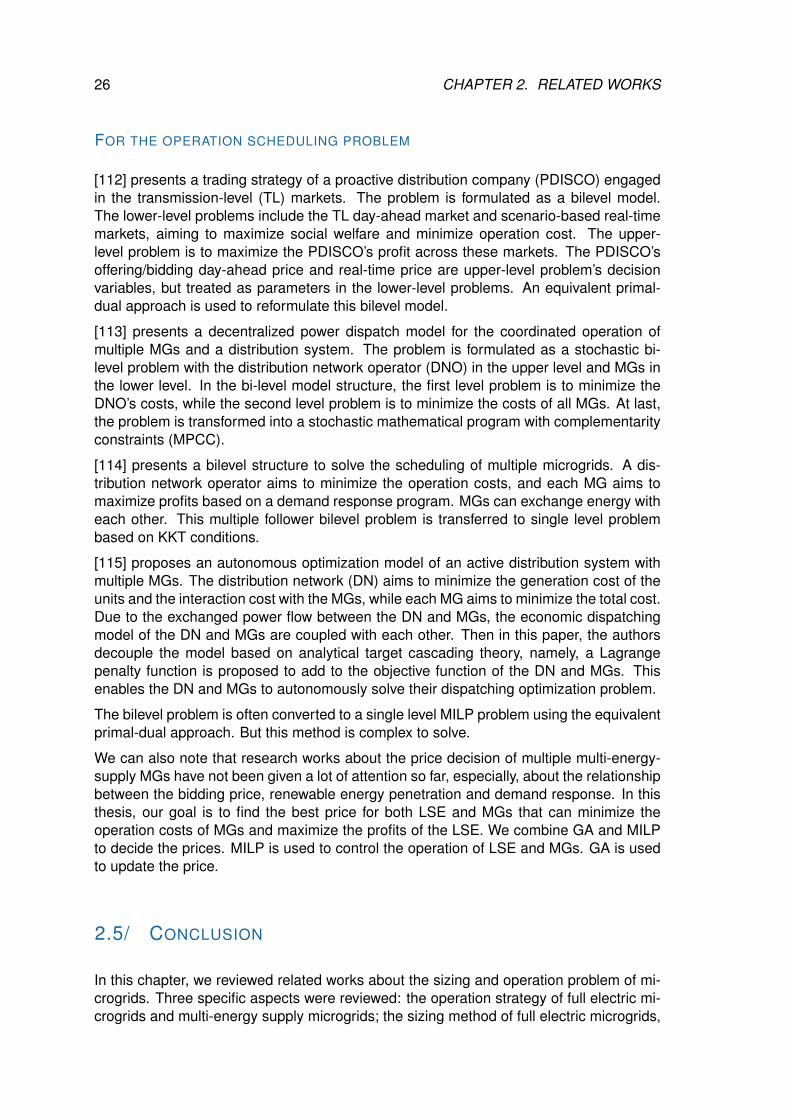
26 CHAPTER 2. RELATED WORKS
FOR THE OPERATION SCHEDULING PROBLEM
[112] presents a trading strategy of a proactive distribution company (PDISCO) engagedin the transmission-level (TL) markets. The problem is formulated as a bilevel model.The lower-level problems include the TL day-ahead market and scenario-based real-timemarkets, aiming to maximize social welfare and minimize operation cost. The upper-level problem is to maximize the PDISCO’s profit across these markets. The PDISCO’soffering/bidding day-ahead price and real-time price are upper-level problem’s decisionvariables, but treated as parameters in the lower-level problems. An equivalent primal-dual approach is used to reformulate this bilevel model.
[113] presents a decentralized power dispatch model for the coordinated operation ofmultiple MGs and a distribution system. The problem is formulated as a stochastic bi-level problem with the distribution network operator (DNO) in the upper level and MGs inthe lower level. In the bi-level model structure, the first level problem is to minimize theDNO’s costs, while the second level problem is to minimize the costs of all MGs. At last,the problem is transformed into a stochastic mathematical program with complementarityconstraints (MPCC).
[114] presents a bilevel structure to solve the scheduling of multiple microgrids. A dis-tribution network operator aims to minimize the operation costs, and each MG aims tomaximize profits based on a demand response program. MGs can exchange energy witheach other. This multiple follower bilevel problem is transferred to single level problembased on KKT conditions.
[115] proposes an autonomous optimization model of an active distribution system withmultiple MGs. The distribution network (DN) aims to minimize the generation cost of theunits and the interaction cost with the MGs, while each MG aims to minimize the total cost.Due to the exchanged power flow between the DN and MGs, the economic dispatchingmodel of the DN and MGs are coupled with each other. Then in this paper, the authorsdecouple the model based on analytical target cascading theory, namely, a Lagrangepenalty function is proposed to add to the objective function of the DN and MGs. Thisenables the DN and MGs to autonomously solve their dispatching optimization problem.
The bilevel problem is often converted to a single level MILP problem using the equivalentprimal-dual approach. But this method is complex to solve.
We can also note that research works about the price decision of multiple multi-energy-supply MGs have not been given a lot of attention so far, especially, about the relationshipbetween the bidding price, renewable energy penetration and demand response. In thisthesis, our goal is to find the best price for both LSE and MGs that can minimize theoperation costs of MGs and maximize the profits of the LSE. We combine GA and MILPto decide the prices. MILP is used to control the operation of LSE and MGs. GA is usedto update the price.
2.5/ CONCLUSION
In this chapter, we reviewed related works about the sizing and operation problem of mi-crogrids. Three specific aspects were reviewed: the operation strategy of full electric mi-crogrids and multi-energy supply microgrids; the sizing method of full electric microgrids,

2.5. CONCLUSION 27
multi-energy supply microgrids and grid-connected microgrids; and the price decisionapproach for grid-connected multiple multi-energy-supply microgrids.
We found that although a large number of papers have been presented to solve themicrogrid sizing problem, there are still some problems that need to be solved. Theseproblems can be concluded as:
1. How to size and operate hydrogen-based microgrids (combining hydrogen storageand battery storage);
2. How to size and operate multi-energy supply microgrids (considering electric-ity/heating/cooling/hydrogen demands);
3. How to size and operate multi-energy supply microgrid considering the electric-ity/gas/heat utility grid;
4. How to decide the prices for grid-connected multiple multi-energy-supply microgrids.
In the following chapters, the solutions to the above problems will be discussed and ex-plained in details.


IICONTRIBUTION
29

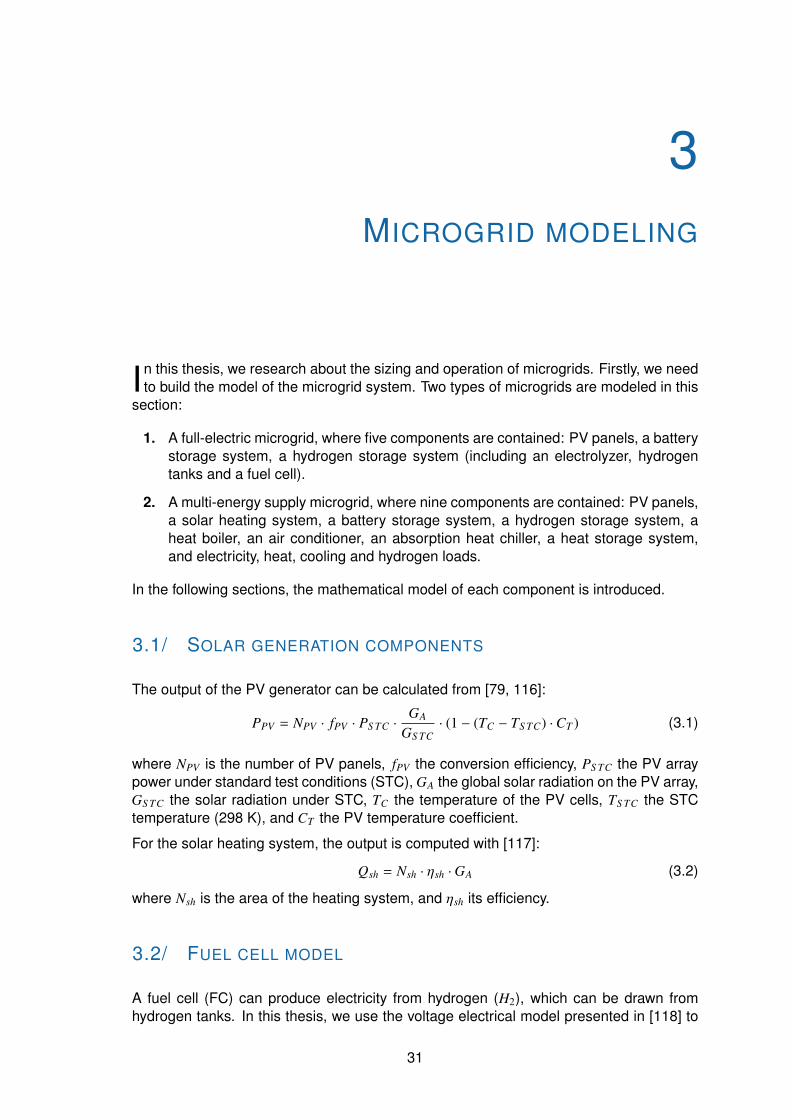
3MICROGRID MODELING
In this thesis, we research about the sizing and operation of microgrids. Firstly, we needto build the model of the microgrid system. Two types of microgrids are modeled in this
section:
1. A full-electric microgrid, where five components are contained: PV panels, a batterystorage system, a hydrogen storage system (including an electrolyzer, hydrogentanks and a fuel cell).
2. A multi-energy supply microgrid, where nine components are contained: PV panels,a solar heating system, a battery storage system, a hydrogen storage system, aheat boiler, an air conditioner, an absorption heat chiller, a heat storage system,and electricity, heat, cooling and hydrogen loads.
In the following sections, the mathematical model of each component is introduced.
3.1/ SOLAR GENERATION COMPONENTS
The output of the PV generator can be calculated from [79, 116]:
PPV = NPV · fPV · PS TC ·GA
GS TC· (1 − (TC − TS TC) ·CT ) (3.1)
where NPV is the number of PV panels, fPV the conversion efficiency, PS TC the PV arraypower under standard test conditions (STC), GA the global solar radiation on the PV array,GS TC the solar radiation under STC, TC the temperature of the PV cells, TS TC the STCtemperature (298 K), and CT the PV temperature coefficient.
For the solar heating system, the output is computed with [117]:
Qsh = Nsh · ηsh ·GA (3.2)
where Nsh is the area of the heating system, and ηsh its efficiency.
3.2/ FUEL CELL MODEL
A fuel cell (FC) can produce electricity from hydrogen (H2), which can be drawn fromhydrogen tanks. In this thesis, we use the voltage electrical model presented in [118] to
31

32 CHAPTER 3. MICROGRID MODELING
describe the characteristic of FC:
V f c = (EOC − r f c · i f c − A · ln(i f c) − m · en·i f c) · N f c (3.3)
where V f c is the FC voltage, EOC is the open-circuit voltage of one cell, i f c is the cur-rent density in one cell, N f c is the number of cells, and n, r f c, A, and m are empiricalcoefficients.
As an PEM FC generates electricity and heat at the same time, the produced heat canbe calculated as in [119]:
Q f c = N f c · (1.48 −V f c
N f c) · I f c (3.4)
Then the hydrogen consumed by the FC is computed using:
nconH2 =
N f cI f c
2FU(3.5)
where F is the Faraday constant, and U is the utilization efficiency of hydrogen in the FC.
From the above equations, we can derive that P f c = f (nconH2 ), where f (.) is a nonlinear
function. In order to reduce the calculation time and obtain a linear model, we use lin-ear regression to simplify this function, without significant loss of model accuracy in thenormal operation zones:
nconH2 = k f c · P f c (3.6)
where k f c is a constant.
In the following, we give an example of PEM FC model based on the above analysis. Themain parameters of the PEM FC model is shown in Tab. 3.1.
Table 3.1: PEM FC parameters.
Fuel cell [19, 21, 118, 76]A 0.03
r f c 2.45 × 10⁻⁴
m 2.11 × 10⁻⁵
n 0.008
The voltage and current characteristic curve of one fuel cell can be seen in Fig. 3.1.
The voltage and power characteristic curve of one fuel cell stack can be seen in Fig.3.2.
The relationship between output power and consumed hydrogen of one fuel cell stackcan be seen in Fig.3.3.
The FC operates as the main power source, which means that it will run for a largenumber of hours, and over time, its performance will decrease. The degradation of thefuel cell must thus be considered [120, 121]. Here, we consider a steady-state lifetimeFC model, where the output current is a constant value, which reduces the degradationof fuel cell. As the FC operates as a long term storage system, cycling loads (loadchanges, start-stop, idling, and high power) will be the main load demands, which willaccelerate the degradation of the fuel cell [122]. But in this first planning stage, the futureoperation states of the fuel cell are unknown, which means that the accelerated factorsof degradation are unknown. In other words, the future operation states can only be
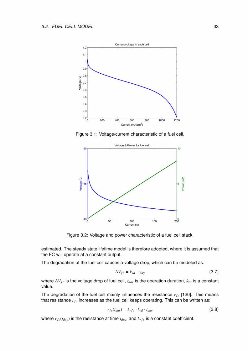
3.2. FUEL CELL MODEL 33
Figure 3.1: Voltage/current characteristic of a fuel cell.
Figure 3.2: Voltage and power characteristic of a fuel cell stack.
estimated. The steady state lifetime model is therefore adopted, where it is assumed thatthe FC will operate at a constant output.
The degradation of the fuel cell causes a voltage drop, which can be modeled as:
∆V f c = kvd · tday (3.7)
where ∆V f c is the voltage drop of fuel cell, tday is the operation duration, kvd is a constantvalue.
The degradation of the fuel cell mainly influences the resistance r f c [120]. This meansthat resistance r f c increases as the fuel cell keeps operating. This can be written as:
r f c(tday) = kr f c · kvd · tday (3.8)
where r f c(tday) is the resistance at time tday, and kr f c is a constant coefficient.
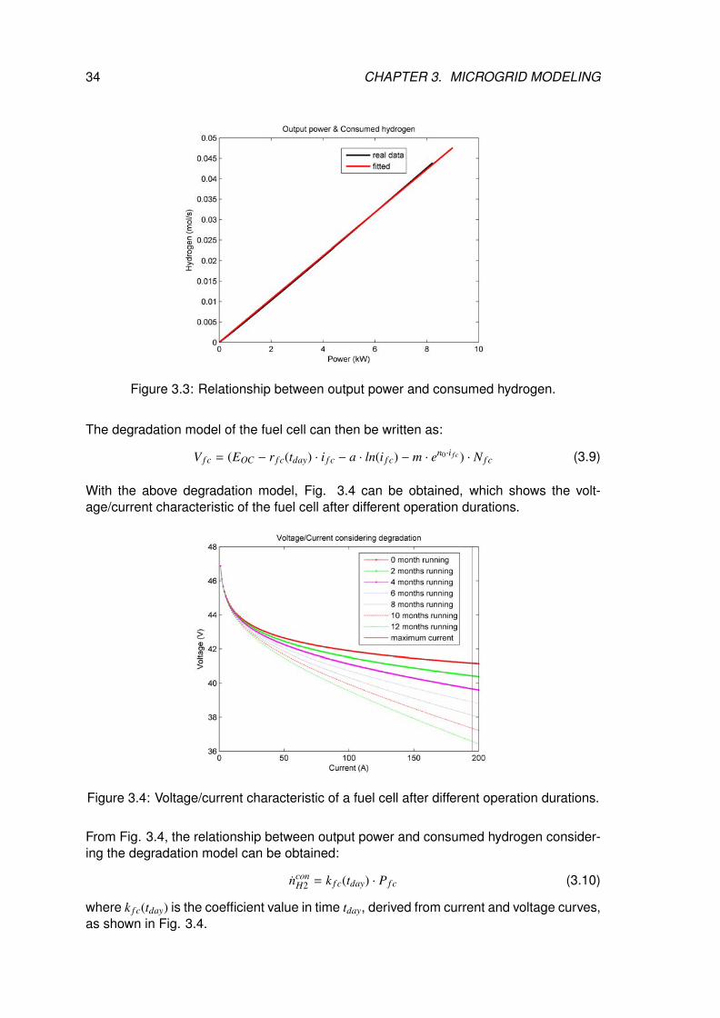
34 CHAPTER 3. MICROGRID MODELING
Figure 3.3: Relationship between output power and consumed hydrogen.
The degradation model of the fuel cell can then be written as:
V f c = (EOC − r f c(tday) · i f c − a · ln(i f c) − m · en0·i f c) · N f c (3.9)
With the above degradation model, Fig. 3.4 can be obtained, which shows the volt-age/current characteristic of the fuel cell after different operation durations.
Figure 3.4: Voltage/current characteristic of a fuel cell after different operation durations.
From Fig. 3.4, the relationship between output power and consumed hydrogen consider-ing the degradation model can be obtained:
nconH2 = k f c(tday) · P f c (3.10)
where k f c(tday) is the coefficient value in time tday, derived from current and voltage curves,as shown in Fig. 3.4.
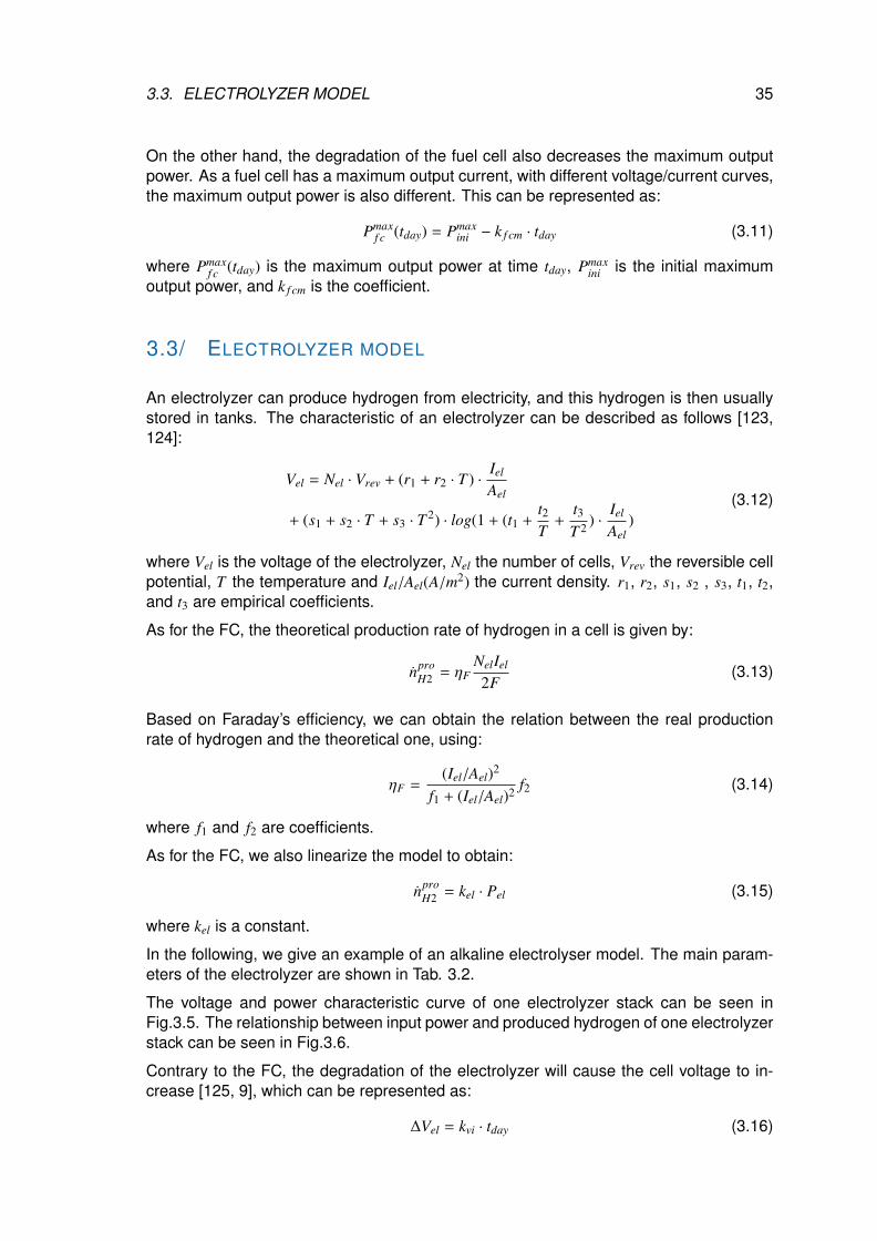
3.3. ELECTROLYZER MODEL 35
On the other hand, the degradation of the fuel cell also decreases the maximum outputpower. As a fuel cell has a maximum output current, with different voltage/current curves,the maximum output power is also different. This can be represented as:
Pmaxf c (tday) = Pmax
ini − k f cm · tday (3.11)
where Pmaxf c (tday) is the maximum output power at time tday, Pmax
ini is the initial maximumoutput power, and k f cm is the coefficient.
3.3/ ELECTROLYZER MODEL
An electrolyzer can produce hydrogen from electricity, and this hydrogen is then usuallystored in tanks. The characteristic of an electrolyzer can be described as follows [123,124]:
Vel = Nel · Vrev + (r1 + r2 · T ) ·Iel
Ael
+ (s1 + s2 · T + s3 · T 2) · log(1 + (t1 +t2T
+t3T 2 ) ·
Iel
Ael)
(3.12)
where Vel is the voltage of the electrolyzer, Nel the number of cells, Vrev the reversible cellpotential, T the temperature and Iel/Ael(A/m2) the current density. r1, r2, s1, s2 , s3, t1, t2,and t3 are empirical coefficients.
As for the FC, the theoretical production rate of hydrogen in a cell is given by:
nproH2 = ηF
NelIel
2F(3.13)
Based on Faraday’s efficiency, we can obtain the relation between the real productionrate of hydrogen and the theoretical one, using:
ηF =(Iel/Ael)2
f1 + (Iel/Ael)2 f2 (3.14)
where f1 and f2 are coefficients.
As for the FC, we also linearize the model to obtain:
nproH2 = kel · Pel (3.15)
where kel is a constant.
In the following, we give an example of an alkaline electrolyser model. The main param-eters of the electrolyzer are shown in Tab. 3.2.
The voltage and power characteristic curve of one electrolyzer stack can be seen inFig.3.5. The relationship between input power and produced hydrogen of one electrolyzerstack can be seen in Fig.3.6.
Contrary to the FC, the degradation of the electrolyzer will cause the cell voltage to in-crease [125, 9], which can be represented as:
∆Vel = kvi · tday (3.16)
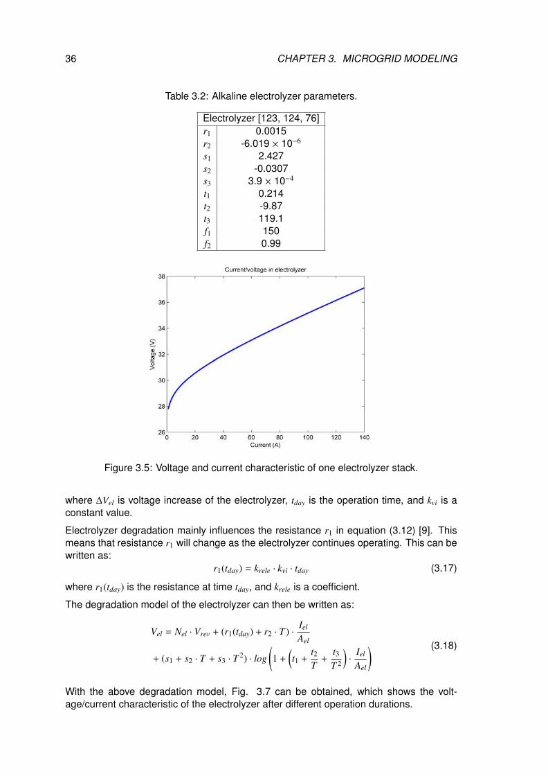
36 CHAPTER 3. MICROGRID MODELING
Table 3.2: Alkaline electrolyzer parameters.
Electrolyzer [123, 124, 76]r1 0.0015r2 -6.019 × 10⁻⁶
s1 2.427s2 -0.0307s3 3.9 × 10⁻⁴
t1 0.214t2 -9.87t3 119.1f1 150f2 0.99
Figure 3.5: Voltage and current characteristic of one electrolyzer stack.
where ∆Vel is voltage increase of the electrolyzer, tday is the operation time, and kvi is aconstant value.
Electrolyzer degradation mainly influences the resistance r1 in equation (3.12) [9]. Thismeans that resistance r1 will change as the electrolyzer continues operating. This can bewritten as:
r1(tday) = krele · kvi · tday (3.17)
where r1(tday) is the resistance at time tday, and krele is a coefficient.
The degradation model of the electrolyzer can then be written as:
Vel = Nel · Vrev + (r1(tday) + r2 · T ) ·Iel
Ael
+ (s1 + s2 · T + s3 · T 2) · log(1 +
(t1 +
t2T
+t3T 2
)·
Iel
Ael
) (3.18)
With the above degradation model, Fig. 3.7 can be obtained, which shows the volt-age/current characteristic of the electrolyzer after different operation durations.
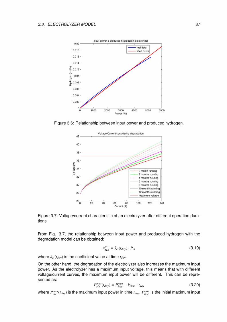
3.3. ELECTROLYZER MODEL 37
Figure 3.6: Relationship between input power and produced hydrogen.
Figure 3.7: Voltage/current characteristic of an electrolyzer after different operation dura-tions.
From Fig. 3.7, the relationship between input power and produced hydrogen with thedegradation model can be obtained:
nproH2 = kel(tday) · Pel (3.19)
where kel(tday) is the coefficient value at time tday.
On the other hand, the degradation of the electrolyzer also increases the maximum inputpower. As the electrolyzer has a maximum input voltage, this means that with differentvoltage/current curves, the maximum input power will be different. This can be repre-sented as:
Pmaxele (tday) = Pmax
inie − kelem · tday (3.20)
where Pmaxele (tday) is the maximum input power in time tday, Pmax
inie is the initial maximum input
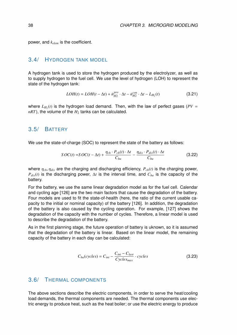
38 CHAPTER 3. MICROGRID MODELING
power, and kelem is the coefficient.
3.4/ HYDROGEN TANK MODEL
A hydrogen tank is used to store the hydrogen produced by the electrolyzer, as well asto supply hydrogen to the fuel cell. We use the level of hydrogen (LOH) to represent thestate of the hydrogen tank:
LOH(t) = LOH(t − ∆t) + nproH2 · ∆t − ncon
H2 · ∆t − LH2(t) (3.21)
where LH2(t) is the hydrogen load demand. Then, with the law of perfect gases (PV =
nRT ), the volume of the H2 tanks can be calculated.
3.5/ BATTERY
We use the state-of-charge (SOC) to represent the state of the battery as follows:
S OC(t) =S OC(t − ∆t) +ηch · Pch(t) · ∆t
Cba−ηdis · Pdis(t) · ∆t
Cba(3.22)
where ηch, ηdis are the charging and discharging efficiency, Pch(t) is the charging power,Pdis(t) is the discharging power, ∆t is the interval time, and Cba is the capacity of thebattery.
For the battery, we use the same linear degradation model as for the fuel cell. Calendarand cycling age [126] are the two main factors that cause the degradation of the battery.Four models are used to fit the state-of-health (here, the ratio of the current usable ca-pacity to the initial or nominal capacity) of the battery [126]. In addition, the degradationof the battery is also caused by the cycling operation. For example, [127] shows thedegradation of the capacity with the number of cycles. Therefore, a linear model is usedto describe the degradation of the battery.
As in the first planning stage, the future operation of battery is uknown, so it is assumedthat the degradation of the battery is linear. Based on the linear model, the remainingcapacity of the battery in each day can be calculated:
Cba(cycles) = Cini −Cini −Clast
Cyclesmax· cycles (3.23)
3.6/ THERMAL COMPONENTS
The above sections describe the electric components, in order to serve the heat/coolingload demands, the thermal components are needed. The thermal components use elec-tric energy to produce heat, such as the heat boiler; or use the electric energy to produce
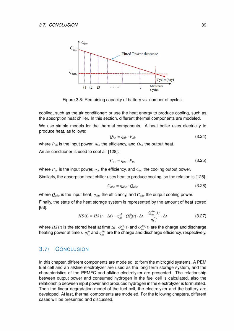
3.7. CONCLUSION 39
Figure 3.8: Remaining capacity of battery vs. number of cycles.
cooling, such as the air conditioner; or use the heat energy to produce cooling, such asthe absorption heat chiller. In this section, different thermal components are modeled.
We use simple models for the thermal components. A heat boiler uses electricity toproduce heat, as follows:
Qhb = ηhb · Phb (3.24)
where Phb is the input power, ηhb the efficiency, and Qhb the output heat.
An air conditioner is used to cool air [128]:
Cac = ηac · Pac (3.25)
where Pac is the input power, ηac the efficiency, and Cac the cooling output power.
Similarly, the absorption heat chiller uses heat to produce cooling, so the relation is [128]:
Cahc = ηahc · Qahc (3.26)
where Qahc is the input heat, ηahc the efficiency, and Cahc the output cooling power.
Finally, the state of the heat storage system is represented by the amount of heat stored[63]:
HS (t) = HS (t − ∆t) + ηchhs · Q
chhs(t) · ∆t −
Qdishs (t)
ηdishs
· ∆t (3.27)
where HS (t) is the stored heat at time ∆t. Qchhs(t) and Qdis
hs (t) are the charge and dischargeheating power at time t. ηch
hs and ηdishs are the charge and discharge efficiency, respectively.
3.7/ CONCLUSION
In this chapter, different components are modeled, to form the microgrid systems. A PEMfuel cell and an alkline electrolyzer are used as the long term storage system, and thecharacteristics of the PEMFC and alkline electrolyzer are presented. The relationshipbetween output power and consumed hydrogen in the fuel cell is calculated, also therelationship between input power and produced hydrogen in the electrolyzer is formulated.Then the linear degradation model of the fuel cell, the electrolyzer and the battery aredeveloped. At last, thermal components are modeled. For the following chapters, differentcases will be presented and discussed.

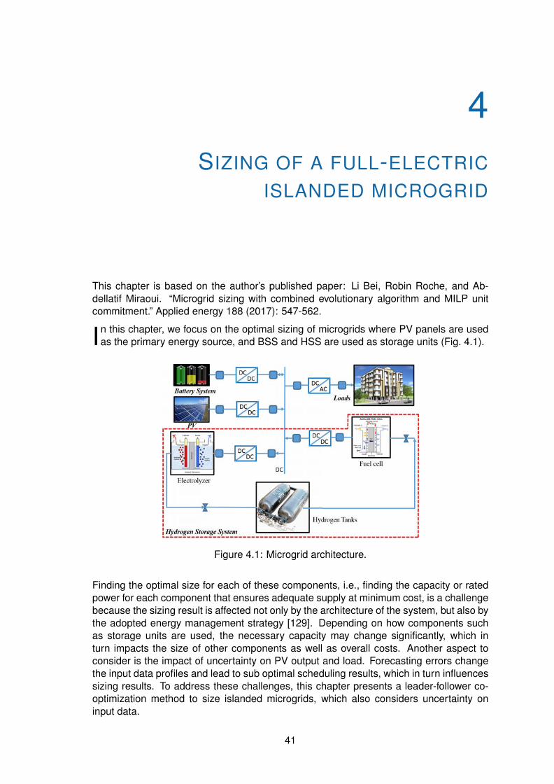
4SIZING OF A FULL-ELECTRIC
ISLANDED MICROGRID
This chapter is based on the author’s published paper: Li Bei, Robin Roche, and Ab-dellatif Miraoui. “Microgrid sizing with combined evolutionary algorithm and MILP unitcommitment.” Applied energy 188 (2017): 547-562.
In this chapter, we focus on the optimal sizing of microgrids where PV panels are usedas the primary energy source, and BSS and HSS are used as storage units (Fig. 4.1).
Figure 4.1: Microgrid architecture.
Finding the optimal size for each of these components, i.e., finding the capacity or ratedpower for each component that ensures adequate supply at minimum cost, is a challengebecause the sizing result is affected not only by the architecture of the system, but also bythe adopted energy management strategy [129]. Depending on how components suchas storage units are used, the necessary capacity may change significantly, which inturn impacts the size of other components as well as overall costs. Another aspect toconsider is the impact of uncertainty on PV output and load. Forecasting errors changethe input data profiles and lead to sub optimal scheduling results, which in turn influencessizing results. To address these challenges, this chapter presents a leader-follower co-optimization method to size islanded microgrids, which also considers uncertainty oninput data.
41
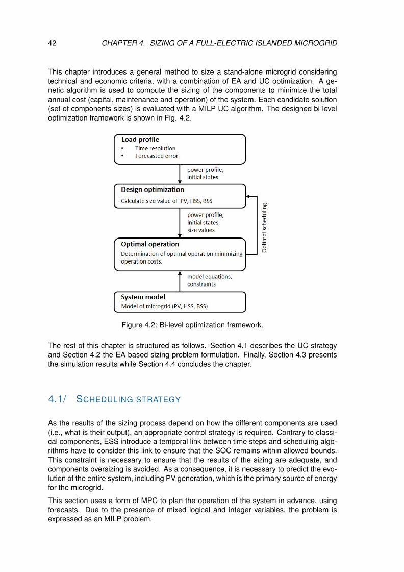
42 CHAPTER 4. SIZING OF A FULL-ELECTRIC ISLANDED MICROGRID
This chapter introduces a general method to size a stand-alone microgrid consideringtechnical and economic criteria, with a combination of EA and UC optimization. A ge-netic algorithm is used to compute the sizing of the components to minimize the totalannual cost (capital, maintenance and operation) of the system. Each candidate solution(set of components sizes) is evaluated with a MILP UC algorithm. The designed bi-leveloptimization framework is shown in Fig. 4.2.
Figure 4.2: Bi-level optimization framework.
The rest of this chapter is structured as follows. Section 4.1 describes the UC strategyand Section 4.2 the EA-based sizing problem formulation. Finally, Section 4.3 presentsthe simulation results while Section 4.4 concludes the chapter.
4.1/ SCHEDULING STRATEGY
As the results of the sizing process depend on how the different components are used(i.e., what is their output), an appropriate control strategy is required. Contrary to classi-cal components, ESS introduce a temporal link between time steps and scheduling algo-rithms have to consider this link to ensure that the SOC remains within allowed bounds.This constraint is necessary to ensure that the results of the sizing are adequate, andcomponents oversizing is avoided. As a consequence, it is necessary to predict the evo-lution of the entire system, including PV generation, which is the primary source of energyfor the microgrid.
This section uses a form of MPC to plan the operation of the system in advance, usingforecasts. Due to the presence of mixed logical and integer variables, the problem isexpressed as an MILP problem.
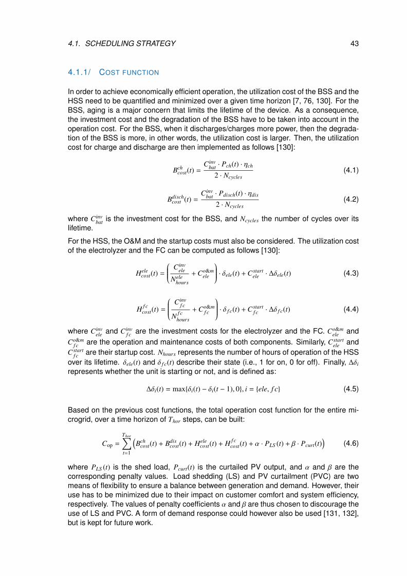
4.1. SCHEDULING STRATEGY 43
4.1.1/ COST FUNCTION
In order to achieve economically efficient operation, the utilization cost of the BSS and theHSS need to be quantified and minimized over a given time horizon [7, 76, 130]. For theBSS, aging is a major concern that limits the lifetime of the device. As a consequence,the investment cost and the degradation of the BSS have to be taken into account in theoperation cost. For the BSS, when it discharges/charges more power, then the degrada-tion of the BSS is more, in other words, the utilization cost is larger. Then, the utilizationcost for charge and discharge are then implemented as follows [130]:
Bchcost(t) =
Cinvbat · Pch(t) · ηch
2 · Ncycles(4.1)
Bdischcost (t) =
Cinvbat · Pdisch(t) · ηdis
2 · Ncycles(4.2)
where Cinvbat is the investment cost for the BSS, and Ncycles the number of cycles over its
lifetime.
For the HSS, the O&M and the startup costs must also be considered. The utilization costof the electrolyzer and the FC can be computed as follows [130]:
Helecost(t) =
Cinvele
Nelehours
+ Co&mele
· δele(t) + Cstartele · ∆δele(t) (4.3)
H f ccost(t) =
Cinvf c
N f chours
+ Co&mf c
· δ f c(t) + Cstartf c · ∆δ f c(t) (4.4)
where Cinvele and Cinv
f c are the investment costs for the electrolyzer and the FC. Co&mele and
Co&mf c are the operation and maintenance costs of both components. Similarly, Cstart
ele andCstart
f c are their startup cost. Nhours represents the number of hours of operation of the HSSover its lifetime. δele(t) and δ f c(t) describe their state (i.e., 1 for on, 0 for off). Finally, ∆δi
represents whether the unit is starting or not, and is defined as:
∆δi(t) = max{δi(t) − δi(t − 1), 0}, i = {ele, f c} (4.5)
Based on the previous cost functions, the total operation cost function for the entire mi-crogrid, over a time horizon of Thor steps, can be built:
Cop =
Thor∑t=1
(Bch
cost(t) + Bdiscost(t) + Hele
cost(t) + H f ccost(t) + α · PLS (t) + β · Pcurt(t)
)(4.6)
where PLS (t) is the shed load, Pcurt(t) is the curtailed PV output, and α and β are thecorresponding penalty values. Load shedding (LS) and PV curtailment (PVC) are twomeans of flexibility to ensure a balance between generation and demand. However, theiruse has to be minimized due to their impact on customer comfort and system efficiency,respectively. The values of penalty coefficients α and β are thus chosen to discourage theuse of LS and PVC. A form of demand response could however also be used [131, 132],but is kept for future work.
44 CHAPTER 4. SIZING OF A FULL-ELECTRIC ISLANDED MICROGRID
4.1.2/ CONSTRAINTS
The operation of the various components is subject to several constraints, as is theislanded operation of the system. In the following equations, i = {ele, f c} and j =
{ele, f c, ch, disch}. First, all component outputs have to be between their minimum andmaximum values:
Pminj ≤ P j(t) ≤ Pmax
j (4.7)
In order to consider the status of each device (on or off), the above equation becomes:
δ j(t) · Pminj ≤Z j(t) ≤ δ j(t) · Pmax
j
Z j(t) = δ j(t) · P j(t)(4.8)
where Z j(t) represents actual outputs of component j at time t.
Due to linearity constraints, this equation can then in turn be transformed into the followingtwo inequalities:
Z j(t) ≤ P j(t) − (1 − δ j(t)) · Pminj
Z j(t) ≥ P j(t) − (1 − δ j(t)) · Pmaxj
(4.9)
Another constraint is that the electrolyzer and the FC should not be working at the sametime, as this would mean charging and discharging at the same time. The HSS is thuseither charging or discharging:
δele(t) + δ f c(t) ≤ 1 (4.10)
A similar constraint is used for the BSS:
δch(t) + δdisch(t) ≤ 1 (4.11)
The SOC and LOH constraints also have to be verified:
S OCmin ≤ S OC(t) ≤ S OCmax (4.12)
LOHminH2≤ LOHH2(t) ≤ LOHmax
H2(4.13)
Then, equation (4.5) can be rewritten as:
∆δi(t) = δi(t) · (1 − δi(t − 1)), i = {ele, f c} (4.14)
From [133], the above nonlinear equation can be transformed into the following linearconstraints:
−δi(t) + ∆δi(t) ≤ 0 (4.15)−(1 − δi(t − 1)) + ∆δi(t) ≤ 0 (4.16)
δi(t) + (1 − δi(t − 1)) − ∆δi(t) ≤ 1 (4.17)
Finally, as the system is islanded, the balance between generation and demand has tobe met at all time steps, so:
PPV (t) − Pcurt(t) − (Pload(t) − PLS (t)) = Zele(t) − Z f c(t) + Zch(t) − Zdis(t) (4.18)
4.2. SIZING ALGORITHM 45
4.1.3/ PROBLEM FORMULATION
Using the above cost function and constraints, the microgrid UC problem can be summa-rized as follows, where S is the set of variables:
minS{Cop} s.t. (3.22), (3.15), (3.6), (3.21), (4.7) − (4.18) (4.19)
4.2/ SIZING ALGORITHM
The scheduling strategy presented in the previous section requires several input vari-ables. Some of these variables correspond to the maximum rating or capacity of eachcomponent, which are the results of the sizing algorithm. Other inputs are parameters setby the user, such as the initial SOC and LOH values, and the penalty coefficients α andβ. The impact of these parameters on results will be discussed in Section 4.3.
4.2.1/ LEADER-FOLLOWER STRUCTURE
The sizing problem aims at finding the optimal size of the PV, BSS, electrolyzer and FCcomponents to achieve the most cost-effective solution over a given time period. LetNPV ∈ NPV, Cbat ∈ Cbat, Vmax
H2∈ VH2 , Pmax
el ∈ Pel, Pmaxf c ∈ Pfc. Set U represent the whole set
of sizing variables, namely, U = NPV ∪ Cbat ∪ VH2 ∪ Pel ∪ Pfc, and U ∈ U.
The problem can be formulated as a leader-follower problem [134]. The leader problem(the sizing problem) is as follows:
minU∈U{F(U)} (4.20)
where F(.) is a function representing the total cost of the system over the simulationduration.
The follower problem (the scheduling problem), is defined as:
minU∗,S{Cop} s.t. (3.22), (3.15), (3.6), (3.21), (4.7) − (4.18) (4.21)
where U∗ is the set of sizing values obtained from the leader.
In other words, the leader first returns a candidate set of values for NPV , Cbat, VmaxH2
, Pmaxel ,
and Pmaxf c . Then the follower uses these values to calculate the total operation cost using
the algorithm described in Section 4.1. Based on this cost information, the leader adjuststhe sizing values until an optimal value that minimizes the overall cost is found.
4.2.2/ LEADER PROBLEM OBJECTIVE FUNCTION
To obtain a valid estimate of the actual cost of the system, operation cost is insufficient ascapital and maintenance costs must also be considered [32, 31, 76]. In order to convertthe initial capital cost to an annual capital cost, the capital recovery factor (CRF) is used[32]:
CRF =r(1 + r)ninv
(1 + r)ninv − 1(4.22)
46 CHAPTER 4. SIZING OF A FULL-ELECTRIC ISLANDED MICROGRID
where r is the real interest rate and ninv is the expected life span of the microgrid.
The total capital cost corresponds to the cost of buying the equipment, given by:
Ccap = CRF · (NPV ·CinvPV + Pmax
f c ·Cinvf c + Pmax
el ·Cinvele + VH2 ·C
invtank + Cbat ·Cinv
bat) (4.23)
where Cinv variables represent the costs of the PV, FC, electrolyzer, hydrogen tanks andbattery components.
Similarly, the annual maintenance cost is given by:
Cmnt = NPV ·CmntPV + VH2 ·C
mnttank + Cbat ·Cmnt
bat (4.24)
where Cmnt variables represent the annual maintenance costs of the PV, hydrogen tanksand battery components. As the O&M cost of the FC and the electrolyzer are consideredin the operation strategy equations (4.3) to (4.4), they are not included in the annual cost.
The fitness function of the leader problem is thus the total cost function F(.) given by:
F = Ccap + Cop + Cmnt (4.25)
Finally, the overall sizing problem can be formulated as:
minU∈U{Ccap + min
U∗,S{Cop} + Cmnt}
s.t. (3.22), (3.15), (3.6), (3.21), (4.7) − (4.18)(4.26)
4.2.3/ SIMULATION PROCESS
In order to obtain the optimal sizing for the system, an MILP-based scheduling algorithmand an EA-based sizing algorithm are combined.
A GA [37, 135] is used to solve the leader problem. GA are based on the natural selec-tion process similar to biological evolution. Operators such as selection, crossover andmutation enable generating candidate solutions. The decision variables of the GA arerounded to the nearest higher value, namely sizing values, and are then used in the MILPalgorithm.
The simulation process is shown in Fig. 4.3
1. A population of N candidate solutions for the GA is randomly initialized.
2. Each of these solutions is then used with the follower problem. The UC MILP op-timization is run. If the solution is infeasible (namely, the MILP problem can not besolved), a new candidate solution is generated.
3. The GA fitness function value is then computed to determine the total cost of eachcandidate solution.
4. The process continues until any stopping criterion is met. An adaptive method isselected for this. Firstly, if the fitness function values for two consecutive steps arethe same, then counter Num is incremented. If Num exceeds a given maximumvalue, the simulation stops as the fitness function is not improving anymore. Thesecond criterion is on the number of iterations, for which a maximum number is set.
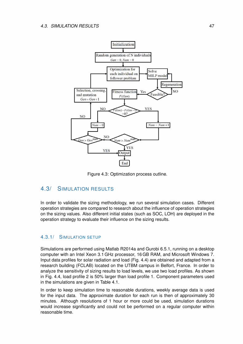
4.3. SIMULATION RESULTS 47
Figure 4.3: Optimization process outline.
4.3/ SIMULATION RESULTS
In order to validate the sizing methodology, we run several simulation cases. Differentoperation strategies are compared to research about the influence of operation strategieson the sizing values. Also different initial states (such as SOC, LOH) are deployed in theoperation strategy to evaluate their influence on the sizing results.
4.3.1/ SIMULATION SETUP
Simulations are performed using Matlab R2014a and Gurobi 6.5.1, running on a desktopcomputer with an Intel Xeon 3.1 GHz processor, 16 GB RAM, and Microsoft Windows 7.Input data profiles for solar radiation and load (Fig. 4.4) are obtained and adapted from aresearch building (FCLAB) located on the UTBM campus in Belfort, France. In order toanalyze the sensitivity of sizing results to load levels, we use two load profiles. As shownin Fig. 4.4, load profile 2 is 50% larger than load profile 1. Component parameters usedin the simulations are given in Table 4.1.
In order to keep simulation time to reasonable durations, weekly average data is usedfor the input data. The approximate duration for each run is then of approximately 30minutes. Although resolutions of 1 hour or more could be used, simulation durationswould increase significantly and could not be performed on a regular computer withinreasonable time.
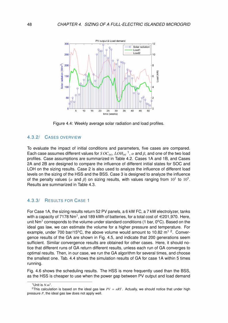
48 CHAPTER 4. SIZING OF A FULL-ELECTRIC ISLANDED MICROGRID
Figure 4.4: Weekly average solar radiation and load profiles.
4.3.2/ CASES OVERVIEW
To evaluate the impact of initial conditions and parameters, five cases are compared.Each case assumes different values for S OCini, LOHini
1, α and β, and one of the two loadprofiles. Case assumptions are summarized in Table 4.2. Cases 1A and 1B, and Cases2A and 2B are designed to compare the influence of different initial states for SOC andLOH on the sizing results. Case 2 is also used to analyze the influence of different loadlevels on the sizing of the HSS and the BSS. Case 3 is designed to analyze the influenceof the penalty values (α and β) on sizing results, with values ranging from 101 to 105.Results are summarized in Table 4.3.
4.3.3/ RESULTS FOR CASE 1
For Case 1A, the sizing results return 52 PV panels, a 6 kW FC, a 7 kW electrolyzer, tankswith a capacity of 7178 Nm3, and 189 kWh of batteries, for a total cost of e201,970. Here,unit Nm3 corresponds to the volume under standard conditions (1 bar, 0oC). Based on theideal gas law, we can estimate the volume for a higher pressure and temperature. Forexample, under 700 bar/15oC, the above volume would amount to 10.82 m3 2. Conver-gence results of the GA are shown in Fig. 4.5, and indicate that 200 generations seemsufficient. Similar convergence results are obtained for other cases. Here, it should no-tice that different runs of GA return different results, unless each run of GA converges tooptimal results. Then, in our case, we run the GA algorithm for several times, and choosethe smallest one. Tab. 4.4 shows the simulation results of GA for case 1A within 5 timesrunning.
Fig. 4.6 shows the scheduling results. The HSS is more frequently used than the BSS,as the HSS is cheaper to use when the power gap between PV output and load demand
1Unit is N.m3.2This calculation is based on the ideal gas law PV = nRT . Actually, we should notice that under high
pressure P, the ideal gas law does not apply well.
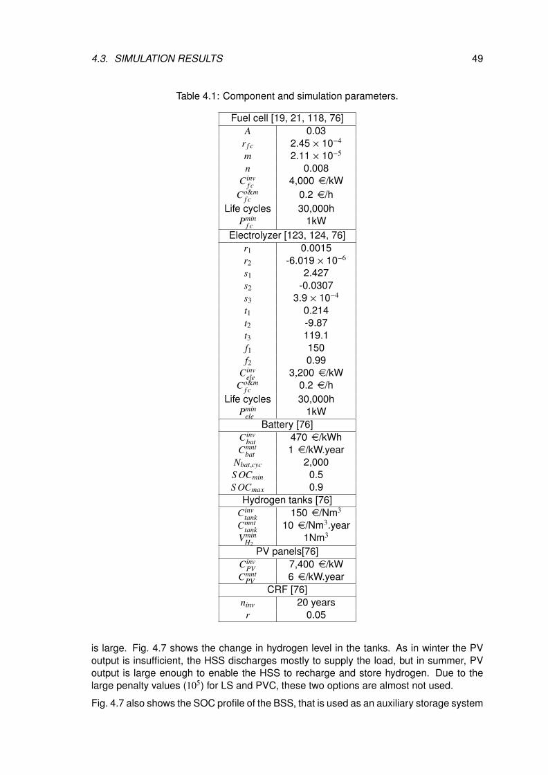
4.3. SIMULATION RESULTS 49
Table 4.1: Component and simulation parameters.
Fuel cell [19, 21, 118, 76]A 0.03
r f c 2.45 × 10⁻⁴
m 2.11 × 10⁻⁵
n 0.008Cinv
f c 4,000 e/kWCo&m
f c 0.2 e/hLife cycles 30,000h
Pminf c 1kW
Electrolyzer [123, 124, 76]r1 0.0015r2 -6.019 × 10⁻⁶
s1 2.427s2 -0.0307s3 3.9 × 10⁻⁴
t1 0.214t2 -9.87t3 119.1f1 150f2 0.99
Cinvele 3,200 e/kW
Co&mf c 0.2 e/h
Life cycles 30,000hPmin
ele 1kWBattery [76]
Cinvbat 470 e/kWh
Cmntbat 1 e/kW.year
Nbat,cyc 2,000S OCmin 0.5S OCmax 0.9
Hydrogen tanks [76]Cinv
tank 150 e/Nm3
Cmnttank 10 e/Nm3.year
VminH2
1Nm3
PV panels[76]Cinv
PV 7,400 e/kWCmnt
PV 6 e/kW.yearCRF [76]
ninv 20 yearsr 0.05
is large. Fig. 4.7 shows the change in hydrogen level in the tanks. As in winter the PVoutput is insufficient, the HSS discharges mostly to supply the load, but in summer, PVoutput is large enough to enable the HSS to recharge and store hydrogen. Due to thelarge penalty values (105) for LS and PVC, these two options are almost not used.
Fig. 4.7 also shows the SOC profile of the BSS, that is used as an auxiliary storage system
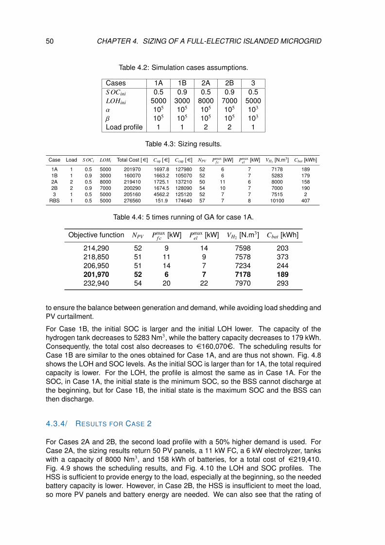
50 CHAPTER 4. SIZING OF A FULL-ELECTRIC ISLANDED MICROGRID
Table 4.2: Simulation cases assumptions.
Cases 1A 1B 2A 2B 3S OCini 0.5 0.9 0.5 0.9 0.5LOHini 5000 3000 8000 7000 5000α 105 105 105 105 103
β 105 105 105 105 103
Load profile 1 1 2 2 1
Table 4.3: Sizing results.
Case Load S OCi LOHi Total Cost [e] Cop [e] Ccap [e] NPV Pmaxf c [kW] Pmax
el [kW] VH2 [N.m3] Cbat [kWh]
1A 1 0.5 5000 201970 1697.8 127980 52 6 7 7178 1891B 1 0.9 3000 160070 1663.2 105070 52 6 7 5283 1792A 2 0.5 8000 219410 1725.1 137210 50 11 6 8000 1582B 2 0.9 7000 200290 1674.5 128090 54 10 7 7000 1903 1 0.5 5000 205160 4562.2 125120 52 7 7 7515 2
RBS 1 0.5 5000 276560 151.9 174640 57 7 8 10100 407
Table 4.4: 5 times running of GA for case 1A.
Objective function NPV Pmaxf c [kW] Pmax
el [kW] VH2 [N.m3] Cbat [kWh]
214,290 52 9 14 7598 203218,850 51 11 9 7578 373206,950 51 14 7 7234 244201,970 52 6 7 7178 189232,940 54 20 22 7970 293
to ensure the balance between generation and demand, while avoiding load shedding andPV curtailment.
For Case 1B, the initial SOC is larger and the initial LOH lower. The capacity of thehydrogen tank decreases to 5283 Nm3, while the battery capacity decreases to 179 kWh.Consequently, the total cost also decreases to e160,070C. The scheduling results forCase 1B are similar to the ones obtained for Case 1A, and are thus not shown. Fig. 4.8shows the LOH and SOC levels. As the initial SOC is larger than for 1A, the total requiredcapacity is lower. For the LOH, the profile is almost the same as in Case 1A. For theSOC, in Case 1A, the initial state is the minimum SOC, so the BSS cannot discharge atthe beginning, but for Case 1B, the initial state is the maximum SOC and the BSS canthen discharge.
4.3.4/ RESULTS FOR CASE 2
For Cases 2A and 2B, the second load profile with a 50% higher demand is used. ForCase 2A, the sizing results return 50 PV panels, a 11 kW FC, a 6 kW electrolyzer, tankswith a capacity of 8000 Nm3, and 158 kWh of batteries, for a total cost of e219,410.Fig. 4.9 shows the scheduling results, and Fig. 4.10 the LOH and SOC profiles. TheHSS is sufficient to provide energy to the load, especially at the beginning, so the neededbattery capacity is lower. However, in Case 2B, the HSS is insufficient to meet the load,so more PV panels and battery energy are needed. We can also see that the rating of
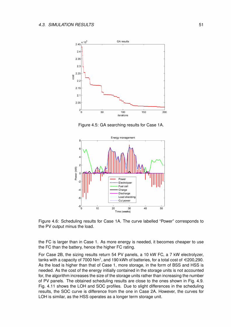
4.3. SIMULATION RESULTS 51
Figure 4.5: GA searching results for Case 1A.
Figure 4.6: Scheduling results for Case 1A. The curve labelled “Power” corresponds tothe PV output minus the load.
the FC is larger than in Case 1. As more energy is needed, it becomes cheaper to usethe FC than the battery, hence the higher FC rating.
For Case 2B, the sizing results return 54 PV panels, a 10 kW FC, a 7 kW electrolyzer,tanks with a capacity of 7000 Nm3, and 190 kWh of batteries, for a total cost of e200,290.As the load is higher than that of Case 1, more storage, in the form of BSS and HSS isneeded. As the cost of the energy initially contained in the storage units is not accountedfor, the algorithm increases the size of the storage units rather than increasing the numberof PV panels. The obtained scheduling results are close to the ones shown in Fig. 4.9.Fig. 4.11 shows the LOH and SOC profiles. Due to slight differences in the schedulingresults, the SOC curve is difference from the one in Case 2A. However, the curves forLOH is similar, as the HSS operates as a longer term storage unit.
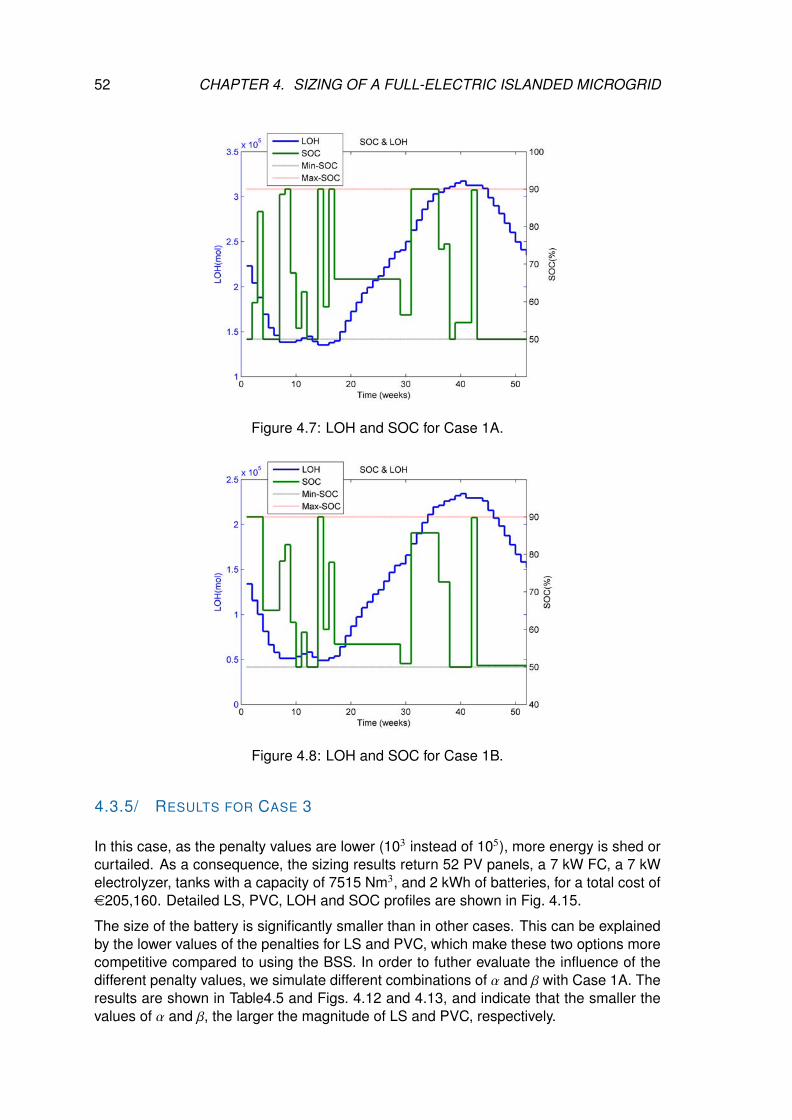
52 CHAPTER 4. SIZING OF A FULL-ELECTRIC ISLANDED MICROGRID
Figure 4.7: LOH and SOC for Case 1A.
Figure 4.8: LOH and SOC for Case 1B.
4.3.5/ RESULTS FOR CASE 3
In this case, as the penalty values are lower (103 instead of 105), more energy is shed orcurtailed. As a consequence, the sizing results return 52 PV panels, a 7 kW FC, a 7 kWelectrolyzer, tanks with a capacity of 7515 Nm3, and 2 kWh of batteries, for a total cost ofe205,160. Detailed LS, PVC, LOH and SOC profiles are shown in Fig. 4.15.
The size of the battery is significantly smaller than in other cases. This can be explainedby the lower values of the penalties for LS and PVC, which make these two options morecompetitive compared to using the BSS. In order to futher evaluate the influence of thedifferent penalty values, we simulate different combinations of α and β with Case 1A. Theresults are shown in Table4.5 and Figs. 4.12 and 4.13, and indicate that the smaller thevalues of α and β, the larger the magnitude of LS and PVC, respectively.
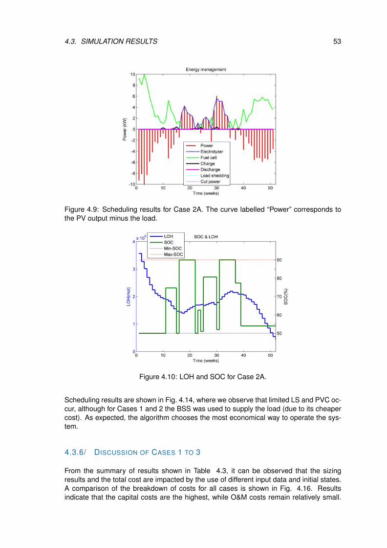
4.3. SIMULATION RESULTS 53
Figure 4.9: Scheduling results for Case 2A. The curve labelled “Power” corresponds tothe PV output minus the load.
Figure 4.10: LOH and SOC for Case 2A.
Scheduling results are shown in Fig. 4.14, where we observe that limited LS and PVC oc-cur, although for Cases 1 and 2 the BSS was used to supply the load (due to its cheapercost). As expected, the algorithm chooses the most economical way to operate the sys-tem.
4.3.6/ DISCUSSION OF CASES 1 TO 3
From the summary of results shown in Table 4.3, it can be observed that the sizingresults and the total cost are impacted by the use of different input data and initial states.A comparison of the breakdown of costs for all cases is shown in Fig. 4.16. Resultsindicate that the capital costs are the highest, while O&M costs remain relatively small.
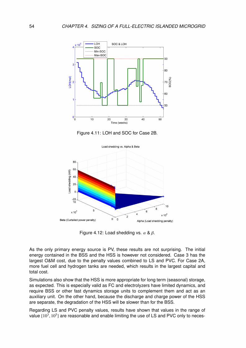
54 CHAPTER 4. SIZING OF A FULL-ELECTRIC ISLANDED MICROGRID
Figure 4.11: LOH and SOC for Case 2B.
Figure 4.12: Load shedding vs. α & β.
As the only primary energy source is PV, these results are not surprising. The initialenergy contained in the BSS and the HSS is however not considered. Case 3 has thelargest O&M cost, due to the penalty values combined to LS and PVC. For Case 2A,more fuel cell and hydrogen tanks are needed, which results in the largest capital andtotal cost.
Simulations also show that the HSS is more appropriate for long term (seasonal) storage,as expected. This is especially valid as FC and electrolyzers have limited dynamics, andrequire BSS or other fast dynamics storage units to complement them and act as anauxiliary unit. On the other hand, because the discharge and charge power of the HSSare separate, the degradation of the HSS will be slower than for the BSS.
Regarding LS and PVC penalty values, results have shown that values in the range ofvalue [103, 105] are reasonable and enable limiting the use of LS and PVC only to neces-
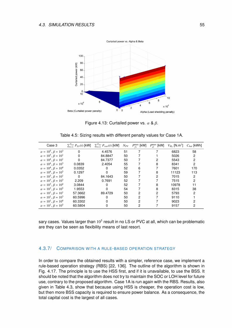
4.3. SIMULATION RESULTS 55
Figure 4.13: Curtailed power vs. α & β.
Table 4.5: Sizing results with different penalty values for Case 1A.
Case 3∑Thor
t=1 PLS (t) [kW]∑Thor
t=1 Pcurt(t) [kW] NPV Pmaxf c [kW] Pmax
el [kW] VH2 [N.m3] Cbat [kWh]
α = 105, β = 103 0 4.4576 51 7 7 6823 58α = 105, β = 101 0 84.8847 50 7 1 5026 2α = 104, β = 101 0 84.7377 50 7 2 5543 2α = 104, β = 103 0.0839 2.4054 55 7 8 8341 2α = 104, β = 104 0.0352 0 52 6 7 7601 170α = 104, β = 105 0.1297 0 59 7 8 11123 113α = 103, β = 101 0 84.1643 50 7 2 7015 2α = 103, β = 103 2.209 0.7691 52 7 7 7515 2α = 103, β = 104 3.0844 0 52 7 8 10978 11α = 103, β = 105 1.9553 0 54 7 8 8315 38α = 101, β = 101 57.3662 89.4729 50 2 2 5793 2α = 101, β = 103 60.5996 0 50 2 7 9110 1α = 101, β = 104 60.3302 0 50 2 7 9023 2α = 101, β = 105 60.5804 0 50 2 7 9157 2
sary cases. Values larger than 105 result in no LS or PVC at all, which can be problematicare they can be seen as flexibility means of last resort.
4.3.7/ COMPARISON WITH A RULE-BASED OPERATION STRATEGY
In order to compare the obtained results with a simpler, reference case, we implement arule-based operation strategy (RBS) [22, 136]. The outline of the algorithm is shown inFig. 4.17. The principle is to use the HSS first, and if it is unavailable, to use the BSS. Itshould be noted that the algorithm does not try to maintain the SOC or LOH level for futureuse, contrary to the proposed algorithm. Case 1A is run again with the RBS. Results, alsogiven in Table 4.3, show that because using HSS is cheaper, the operation cost is low,but then more BSS capacity is required to ensure power balance. As a consequence, thetotal capital cost is the largest of all cases.
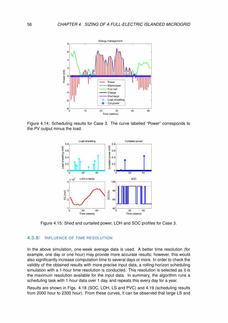
56 CHAPTER 4. SIZING OF A FULL-ELECTRIC ISLANDED MICROGRID
Figure 4.14: Scheduling results for Case 3. The curve labelled “Power” corresponds tothe PV output minus the load.
Figure 4.15: Shed and curtailed power, LOH and SOC profiles for Case 3.
4.3.8/ INFLUENCE OF TIME RESOLUTION
In the above simulation, one-week average data is used. A better time resolution (forexample, one day or one hour) may provide more accurate results; however, this wouldalso significantly increase computation time to several days or more. In order to check thevalidity of the obtained results with more precise input data, a rolling-horizon schedulingsimulation with a 1-hour time resolution is conducted. This resolution is selected as it isthe maximum resolution available for the input data. In summary, the algorithm runs ascheduling task with 1-hour data over 1 day, and repeats this every day for a year.
Results are shown in Figs. 4.18 (SOC, LOH, LS and PVC) and 4.19 (scheduling resultsfrom 2000 hour to 2300 hour). From these curves, it can be observed that large LS and
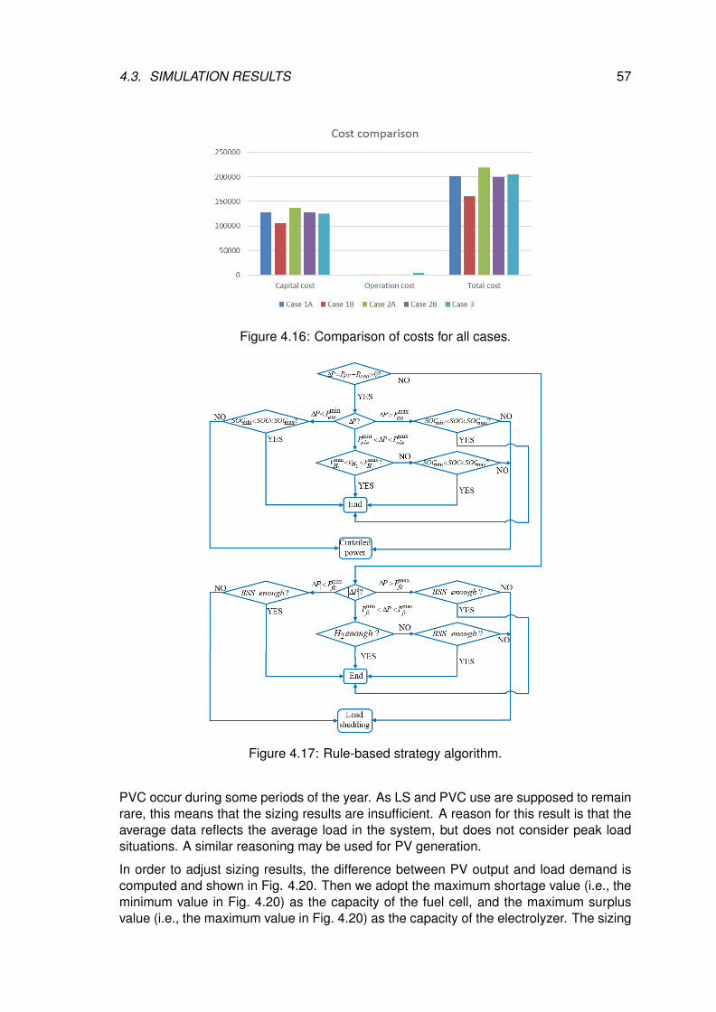
4.3. SIMULATION RESULTS 57
Figure 4.16: Comparison of costs for all cases.
Figure 4.17: Rule-based strategy algorithm.
PVC occur during some periods of the year. As LS and PVC use are supposed to remainrare, this means that the sizing results are insufficient. A reason for this result is that theaverage data reflects the average load in the system, but does not consider peak loadsituations. A similar reasoning may be used for PV generation.
In order to adjust sizing results, the difference between PV output and load demand iscomputed and shown in Fig. 4.20. Then we adopt the maximum shortage value (i.e., theminimum value in Fig. 4.20) as the capacity of the fuel cell, and the maximum surplusvalue (i.e., the maximum value in Fig. 4.20) as the capacity of the electrolyzer. The sizing
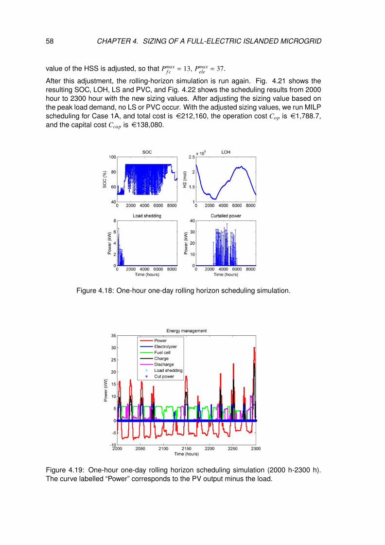
58 CHAPTER 4. SIZING OF A FULL-ELECTRIC ISLANDED MICROGRID
value of the HSS is adjusted, so that Pmaxf c = 13, Pmax
ele = 37.
After this adjustment, the rolling-horizon simulation is run again. Fig. 4.21 shows theresulting SOC, LOH, LS and PVC, and Fig. 4.22 shows the scheduling results from 2000hour to 2300 hour with the new sizing values. After adjusting the sizing value based onthe peak load demand, no LS or PVC occur. With the adjusted sizing values, we run MILPscheduling for Case 1A, and total cost is e212,160, the operation cost Cop is e1,788.7,and the capital cost Ccap is e138,080.
Figure 4.18: One-hour one-day rolling horizon scheduling simulation.
Figure 4.19: One-hour one-day rolling horizon scheduling simulation (2000 h-2300 h).The curve labelled “Power” corresponds to the PV output minus the load.
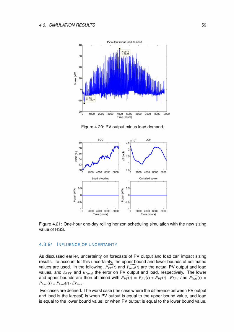
4.3. SIMULATION RESULTS 59
Figure 4.20: PV output minus load demand.
Figure 4.21: One-hour one-day rolling horizon scheduling simulation with the new sizingvalue of HSS.
4.3.9/ INFLUENCE OF UNCERTAINTY
As discussed earlier, uncertainty on forecasts of PV output and load can impact sizingresults. To account for this uncertainty, the upper bound and lower bounds of estimatedvalues are used. In the following, ˜PPV (t) and ˜Pload(t) are the actual PV output and loadvalues, and ErPV and Erload the error on PV output and load, respectively. The lowerand upper bounds are then obtained with ˜PPV (t) = PPV (t) ± PPV (t) · ErPV and ˜Pload(t) =
Pload(t) ± Pload(t) · Erload.
Two cases are defined. The worst case (the case where the difference between PV outputand load is the largest) is when PV output is equal to the upper bound value, and loadis equal to the lower bound value; or when PV output is equal to the lower bound value,
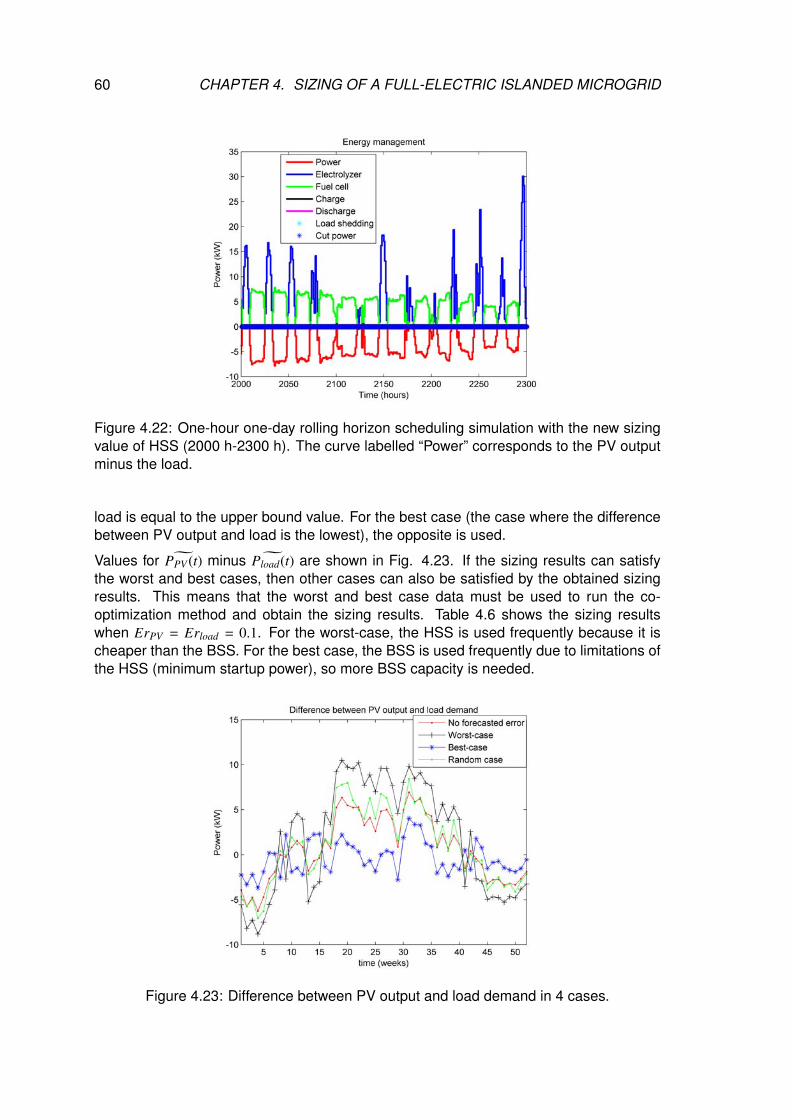
60 CHAPTER 4. SIZING OF A FULL-ELECTRIC ISLANDED MICROGRID
Figure 4.22: One-hour one-day rolling horizon scheduling simulation with the new sizingvalue of HSS (2000 h-2300 h). The curve labelled “Power” corresponds to the PV outputminus the load.
load is equal to the upper bound value. For the best case (the case where the differencebetween PV output and load is the lowest), the opposite is used.
Values for ˜PPV (t) minus ˜Pload(t) are shown in Fig. 4.23. If the sizing results can satisfythe worst and best cases, then other cases can also be satisfied by the obtained sizingresults. This means that the worst and best case data must be used to run the co-optimization method and obtain the sizing results. Table 4.6 shows the sizing resultswhen ErPV = Erload = 0.1. For the worst-case, the HSS is used frequently because it ischeaper than the BSS. For the best case, the BSS is used frequently due to limitations ofthe HSS (minimum startup power), so more BSS capacity is needed.
Figure 4.23: Difference between PV output and load demand in 4 cases.

4.4. CONCLUSION 61
Table 4.6: Sizing results considering uncertainty. The worst case is defined as the casewhere the difference between PV output and load is the largest, and the lowest for thebest case.
Case Total Cost [e] Cop [e] Ccap [e] NPV Pmaxf c [kW] Pmax
el [kW] VH2 [N.m3] Cbat [kWh]
Worst case 279270 1761.7 166960 50 8 8 11022 11Best case 174400 1617.2 113450 50 6 6 5875 269
4.4/ CONCLUSION
In this chapter, we presented a methodology to determine the optimal sizing for a stand-alone microgrid. This methodology combines an EA for sizing and MILP for scheduling,and enables considering advanced energy management strategies, capable of antici-pating decisions (especially with respect to storage), compared to classical rule-basedapproaches. Results showed that the operation strategy, initial conditions, time resolutionas well as uncertainty on input data influence the sizing of the components, and conse-quently the total cost of the microgrid. A comparison with a rule-based operation strategywas run, and sizing results show that co-optimization method performs better. A rolling-horizon simulation was used to adjust the sizing values due to the influence of input datatime resolution. At last, forecasting errors are taken into account using a robust method,to further adjust sizing results. With the proposed method and complements, the pro-posed method can therefore be used for economically sizing a microgrid containing PVpanels, a BSS and an HSS.
For the co-optimization sizing method, the main limitation is the run time when the timeresolution of forecasted load profiles is increasing. For example, when the time resolutionincreases from one week to one hour, then the time horizon of the operation optimizationincreases from 52 to 8760 3. It will take much time to solve this large optimization problem.
3In our sizing problem, the time range is one year, so there are 52 weeks, 365 days, 8760 hours.

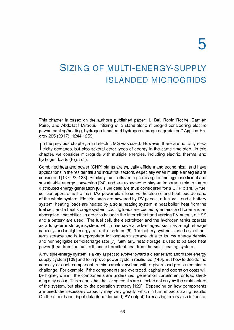
5SIZING OF MULTI-ENERGY-SUPPLY
ISLANDED MICROGRIDS
This chapter is based on the author’s published paper: Li Bei, Robin Roche, DamienPaire, and Abdellatif Miraoui. “Sizing of a stand-alone microgrid considering electricpower, cooling/heating, hydrogen loads and hydrogen storage degradation.” Applied En-ergy 205 (2017): 1244-1259.
In the previous chapter, a full electric MG was sized. However, there are not only elec-tricity demands, but also several other types of energy in the same time step. In this
chapter, we consider microgrids with multiple energies, including electric, thermal andhydrogen loads (Fig. 5.1).
Combined heat and power (CHP) plants are typically efficient and economical, and haveapplications in the residential and industrial sectors, especially when multiple energies areconsidered [137, 23, 138]. Similarly, fuel cells are a promising technology for efficient andsustainable energy conversion [24], and are expected to play an important role in futuredistributed energy generation [6]. Fuel cells are thus considered for a CHP plant. A fuelcell can operate as the main MG power plant to serve the electric and heat load demandof the whole system. Electric loads are powered by PV panels, a fuel cell, and a batterysystem; heating loads are heated by a solar heating system, a heat boiler, heat from thefuel cell, and a heat storage system; cooling loads are cooled by an air conditioner and anabsorption heat chiller. In order to balance the intermittent and varying PV output, a HSSand a battery are used. The fuel cell, the electrolyzer and the hydrogen tanks operateas a long-term storage system, which has several advantages, such as a high storagecapacity, and a high energy per unit of volume [5]. The battery system is used as a short-term storage and is inappropriate for long-term storage, due to its low energy densityand nonnegligible self-discharge rate [7]. Similarly, heat storage is used to balance heatpower (heat from the fuel cell, and intermittent heat from the solar heating system).
A multiple-energy system is a key aspect to evolve toward a cleaner and affordable energysupply system [139] and to improve power system resilience [140]. But how to decide thecapacity of each component in this complex system with a given load profile remains achallenge. For example, if the components are oversized, capital and operation costs willbe higher, while if the components are undersized, generation curtailment or load shed-ding may occur. This means that the sizing results are affected not only by the architectureof the system, but also by the operation strategy [129]. Depending on how componentsare used, the necessary capacity may vary greatly, which in turn impacts sizing results.On the other hand, input data (load demand, PV output) forecasting errors also influence
63
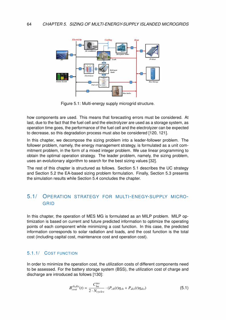
64 CHAPTER 5. SIZING OF MULTI-ENERGY-SUPPLY ISLANDED MICROGRIDS
Figure 5.1: Multi-energy supply microgrid structure.
how components are used. This means that forecasting errors must be considered. Atlast, due to the fact that the fuel cell and the electrolyzer are used as a storage system, asoperation time goes, the performance of the fuel cell and the electrolyzer can be expectedto decrease, so this degradation process must also be considered [120, 121].
In this chapter, we decompose the sizing problem into a leader-follower problem. Thefollower problem, namely, the energy management strategy, is formulated as a unit com-mitment problem, in the form of a mixed integer problem. We use linear programming toobtain the optimal operation strategy. The leader problem, namely, the sizing problem,uses an evolutionary algorithm to search for the best sizing values [32].
The rest of this chapter is structured as follows. Section 5.1 describes the UC strategyand Section 5.2 the EA-based sizing problem formulation. Finally, Section 5.3 presentsthe simulation results while Section 5.4 concludes the chapter.
5.1/ OPERATION STRATEGY FOR MULTI-ENEGY-SUPPLY MICRO-GRID
In this chapter, the operation of MES MG is formulated as an MILP problem. MILP op-timization is based on current and future predicted information to optimize the operatingpoints of each component while minimizing a cost function. In this case, the predictedinformation corresponds to solar radiation and loads, and the cost function is the totalcost (including capital cost, maintenance cost and operation cost).
5.1.1/ COST FUNCTION
In order to minimize the operation cost, the utilization costs of different components needto be assessed. For the battery storage system (BSS), the utilization cost of charge anddischarge are introduced as follows [130]:
Bch,discost (t) =
Cinvba
2 · Ncycles· (Pch(t)ηch + Pdis(t)ηdis) (5.1)
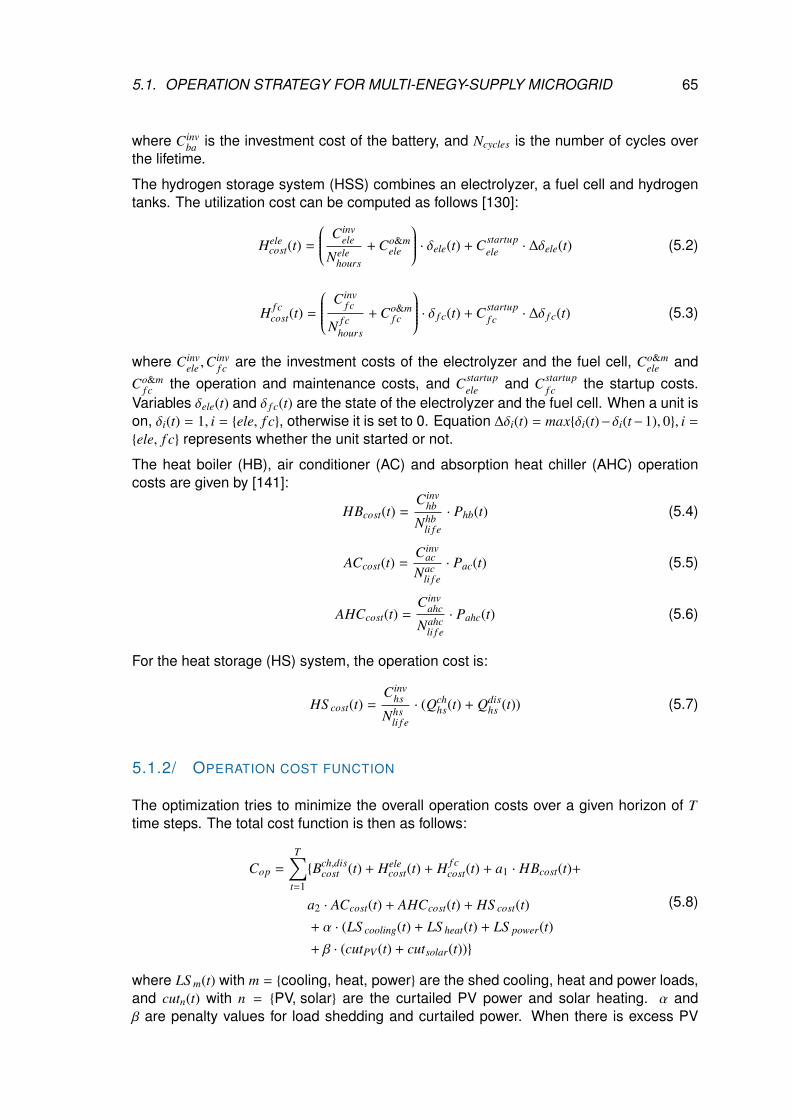
5.1. OPERATION STRATEGY FOR MULTI-ENEGY-SUPPLY MICROGRID 65
where Cinvba is the investment cost of the battery, and Ncycles is the number of cycles over
the lifetime.
The hydrogen storage system (HSS) combines an electrolyzer, a fuel cell and hydrogentanks. The utilization cost can be computed as follows [130]:
Helecost(t) =
Cinvele
Nelehours
+ Co&mele
· δele(t) + Cstartupele · ∆δele(t) (5.2)
H f ccost(t) =
Cinvf c
N f chours
+ Co&mf c
· δ f c(t) + Cstartupf c · ∆δ f c(t) (5.3)
where Cinvele ,C
invf c are the investment costs of the electrolyzer and the fuel cell, Co&m
ele andCo&m
f c the operation and maintenance costs, and Cstartupele and Cstartup
f c the startup costs.Variables δele(t) and δ f c(t) are the state of the electrolyzer and the fuel cell. When a unit ison, δi(t) = 1, i = {ele, f c}, otherwise it is set to 0. Equation ∆δi(t) = max{δi(t)−δi(t−1), 0}, i =
{ele, f c} represents whether the unit started or not.
The heat boiler (HB), air conditioner (AC) and absorption heat chiller (AHC) operationcosts are given by [141]:
HBcost(t) =Cinv
hb
Nhbli f e
· Phb(t) (5.4)
ACcost(t) =Cinv
ac
Nacli f e· Pac(t) (5.5)
AHCcost(t) =Cinv
ahc
Nahcli f e
· Pahc(t) (5.6)
For the heat storage (HS) system, the operation cost is:
HS cost(t) =Cinv
hs
Nhsli f e
· (Qchhs(t) + Qdis
hs (t)) (5.7)
5.1.2/ OPERATION COST FUNCTION
The optimization tries to minimize the overall operation costs over a given horizon of Ttime steps. The total cost function is then as follows:
Cop =
T∑t=1
{Bch,discost (t) + Hele
cost(t) + H f ccost(t) + a1 · HBcost(t)+
a2 · ACcost(t) + AHCcost(t) + HS cost(t)
+ α · (LS cooling(t) + LS heat(t) + LS power(t)
+ β · (cutPV (t) + cutsolar(t))}
(5.8)
where LS m(t) with m = {cooling, heat, power} are the shed cooling, heat and power loads,and cutn(t) with n = {PV, solar} are the curtailed PV power and solar heating. α andβ are penalty values for load shedding and curtailed power. When there is excess PV
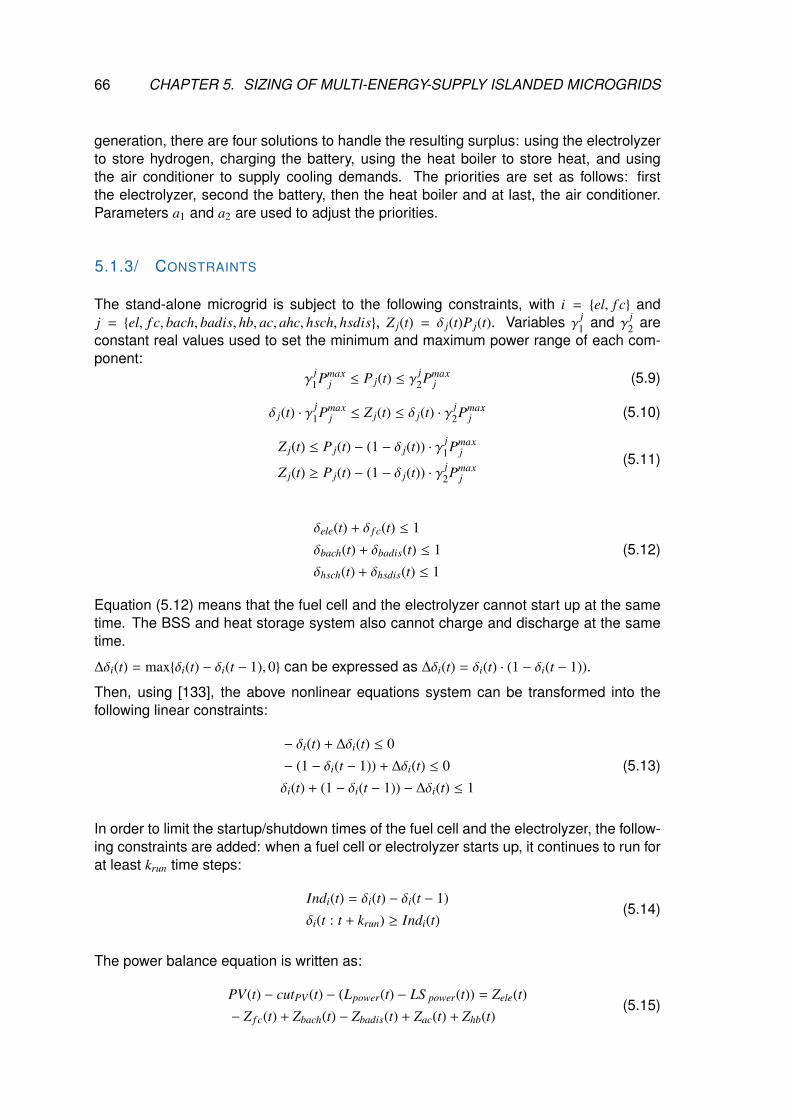
66 CHAPTER 5. SIZING OF MULTI-ENERGY-SUPPLY ISLANDED MICROGRIDS
generation, there are four solutions to handle the resulting surplus: using the electrolyzerto store hydrogen, charging the battery, using the heat boiler to store heat, and usingthe air conditioner to supply cooling demands. The priorities are set as follows: firstthe electrolyzer, second the battery, then the heat boiler and at last, the air conditioner.Parameters a1 and a2 are used to adjust the priorities.
5.1.3/ CONSTRAINTS
The stand-alone microgrid is subject to the following constraints, with i = {el, f c} andj = {el, f c, bach, badis, hb, ac, ahc, hsch, hsdis}, Z j(t) = δ j(t)P j(t). Variables γ
j1 and γ
j2 are
constant real values used to set the minimum and maximum power range of each com-ponent:
γj1Pmax
j ≤ P j(t) ≤ γj2Pmax
j (5.9)
δ j(t) · γj1Pmax
j ≤ Z j(t) ≤ δ j(t) · γj2Pmax
j (5.10)
Z j(t) ≤ P j(t) − (1 − δ j(t)) · γj1Pmax
j
Z j(t) ≥ P j(t) − (1 − δ j(t)) · γj2Pmax
j
(5.11)
δele(t) + δ f c(t) ≤ 1
δbach(t) + δbadis(t) ≤ 1
δhsch(t) + δhsdis(t) ≤ 1
(5.12)
Equation (5.12) means that the fuel cell and the electrolyzer cannot start up at the sametime. The BSS and heat storage system also cannot charge and discharge at the sametime.
∆δi(t) = max{δi(t) − δi(t − 1), 0} can be expressed as ∆δi(t) = δi(t) · (1 − δi(t − 1)).
Then, using [133], the above nonlinear equations system can be transformed into thefollowing linear constraints:
− δi(t) + ∆δi(t) ≤ 0
− (1 − δi(t − 1)) + ∆δi(t) ≤ 0
δi(t) + (1 − δi(t − 1)) − ∆δi(t) ≤ 1
(5.13)
In order to limit the startup/shutdown times of the fuel cell and the electrolyzer, the follow-ing constraints are added: when a fuel cell or electrolyzer starts up, it continues to run forat least krun time steps:
Indi(t) = δi(t) − δi(t − 1)
δi(t : t + krun) ≥ Indi(t)(5.14)
The power balance equation is written as:
PV(t) − cutPV (t) − (Lpower(t) − LS power(t)) = Zele(t)
− Z f c(t) + Zbach(t) − Zbadis(t) + Zac(t) + Zhb(t)(5.15)
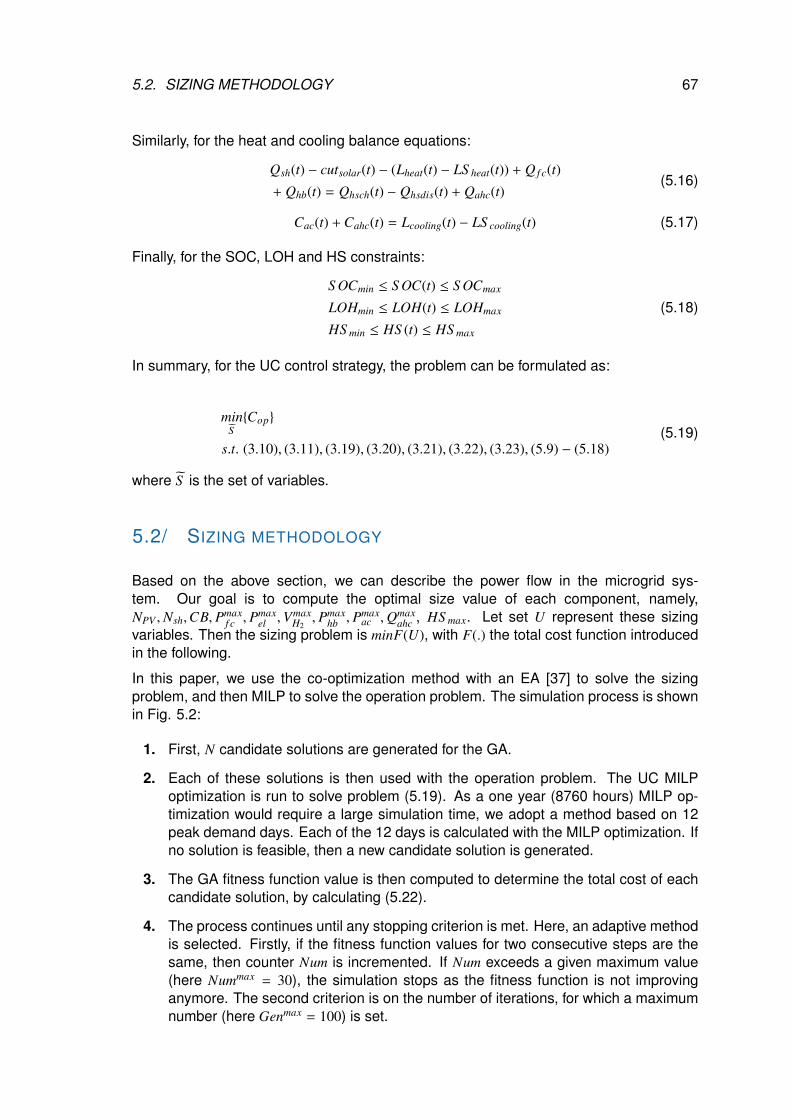
5.2. SIZING METHODOLOGY 67
Similarly, for the heat and cooling balance equations:
Qsh(t) − cutsolar(t) − (Lheat(t) − LS heat(t)) + Q f c(t)
+ Qhb(t) = Qhsch(t) − Qhsdis(t) + Qahc(t)(5.16)
Cac(t) + Cahc(t) = Lcooling(t) − LS cooling(t) (5.17)
Finally, for the SOC, LOH and HS constraints:
S OCmin ≤ S OC(t) ≤ S OCmax
LOHmin ≤ LOH(t) ≤ LOHmax
HS min ≤ HS (t) ≤ HS max
(5.18)
In summary, for the UC control strategy, the problem can be formulated as:
minS{Cop}
s.t. (3.10), (3.11), (3.19), (3.20), (3.21), (3.22), (3.23), (5.9) − (5.18)(5.19)
where S is the set of variables.
5.2/ SIZING METHODOLOGY
Based on the above section, we can describe the power flow in the microgrid sys-tem. Our goal is to compute the optimal size value of each component, namely,NPV ,Nsh,CB, Pmax
f c , Pmaxel ,Vmax
H2, Pmax
hb , Pmaxac ,Qmax
ahc , HS max. Let set U represent these sizingvariables. Then the sizing problem is minF(U), with F(.) the total cost function introducedin the following.
In this paper, we use the co-optimization method with an EA [37] to solve the sizingproblem, and then MILP to solve the operation problem. The simulation process is shownin Fig. 5.2:
1. First, N candidate solutions are generated for the GA.
2. Each of these solutions is then used with the operation problem. The UC MILPoptimization is run to solve problem (5.19). As a one year (8760 hours) MILP op-timization would require a large simulation time, we adopt a method based on 12peak demand days. Each of the 12 days is calculated with the MILP optimization. Ifno solution is feasible, then a new candidate solution is generated.
3. The GA fitness function value is then computed to determine the total cost of eachcandidate solution, by calculating (5.22).
4. The process continues until any stopping criterion is met. Here, an adaptive methodis selected. Firstly, if the fitness function values for two consecutive steps are thesame, then counter Num is incremented. If Num exceeds a given maximum value(here Nummax = 30), the simulation stops as the fitness function is not improvinganymore. The second criterion is on the number of iterations, for which a maximumnumber (here Genmax = 100) is set.
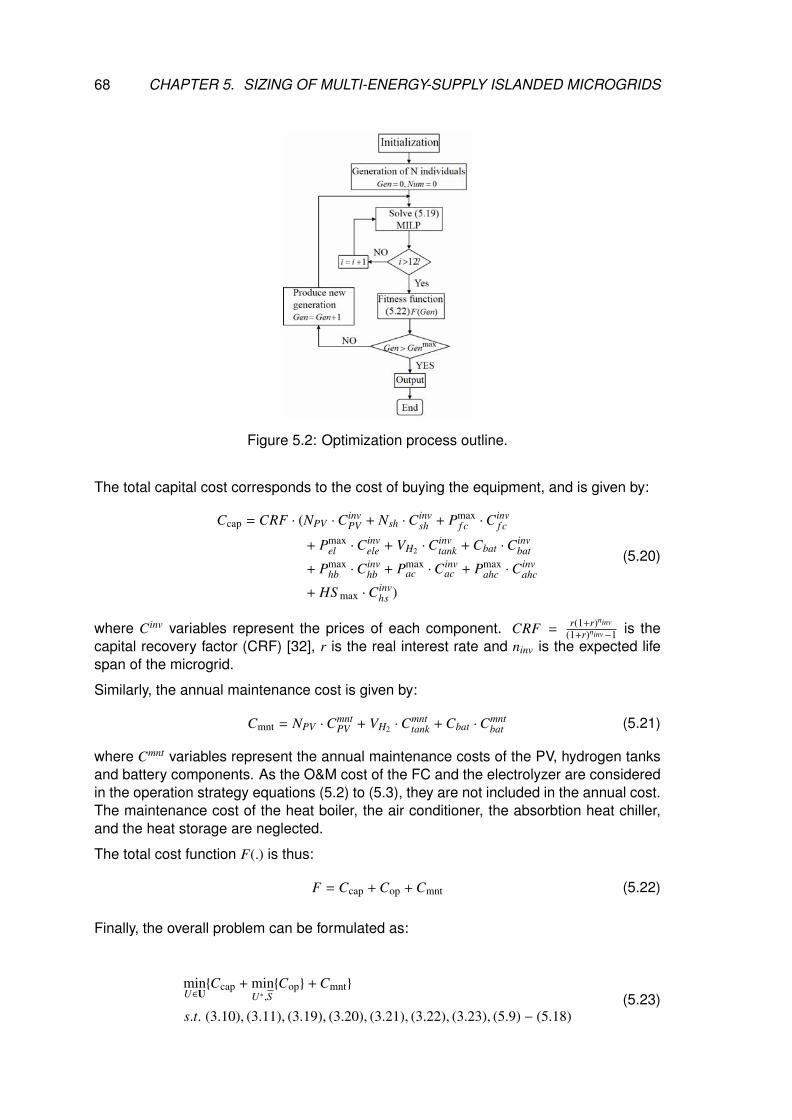
68 CHAPTER 5. SIZING OF MULTI-ENERGY-SUPPLY ISLANDED MICROGRIDS
Figure 5.2: Optimization process outline.
The total capital cost corresponds to the cost of buying the equipment, and is given by:
Ccap = CRF · (NPV ·CinvPV + Nsh ·Cinv
sh + Pmaxf c ·C
invf c
+ Pmaxel ·C
invele + VH2 ·C
invtank + Cbat ·Cinv
bat
+ Pmaxhb ·C
invhb + Pmax
ac ·Cinvac + Pmax
ahc ·Cinvahc
+ HS max ·Cinvhs )
(5.20)
where Cinv variables represent the prices of each component. CRF =r(1+r)ninv
(1+r)ninv−1 is thecapital recovery factor (CRF) [32], r is the real interest rate and ninv is the expected lifespan of the microgrid.
Similarly, the annual maintenance cost is given by:
Cmnt = NPV ·CmntPV + VH2 ·C
mnttank + Cbat ·Cmnt
bat (5.21)
where Cmnt variables represent the annual maintenance costs of the PV, hydrogen tanksand battery components. As the O&M cost of the FC and the electrolyzer are consideredin the operation strategy equations (5.2) to (5.3), they are not included in the annual cost.The maintenance cost of the heat boiler, the air conditioner, the absorbtion heat chiller,and the heat storage are neglected.
The total cost function F(.) is thus:
F = Ccap + Cop + Cmnt (5.22)
Finally, the overall problem can be formulated as:
minU∈U{Ccap + min
U∗,S{Cop} + Cmnt}
s.t. (3.10), (3.11), (3.19), (3.20), (3.21), (3.22), (3.23), (5.9) − (5.18)(5.23)
5.3. SIMULATION RESULTS 69
5.3/ SIMULATION RESULTS
5.3.1/ SYSTEM SETUP
In order to research about the influence of different operation strategies, we set up threedifferent strategies, shown in Table 5.1. Strategies S1 and S3 are used to compare theinfluence of minimum startup power of the fuel cell, the electrolyzer and the heat boiler onthe sizing results. Strategies S2 and S3 are used to compare different operation durationsof the fuel cell and the electrolyzer on the sizing results.
Table 5.1: Three different operation strategies.
Strategy γ{ f c,ele}1 γ
{ f c,ele}2 krun[h]
S1 0.1 1 3S2 0.5 1 5S3 0.5 1 3
The other main operation parameters are shown in Table 5.2, where ”hb” means heatboiler, ”ac” means air conditioner, ”ahc” means absorbtion heat chiller, ”hy” means hydro-gen tanks, and ”hs” means heat storage system.
Table 5.2: Simulation parameters.
Components γ1 γ2
hb 0 1ac 0.1 0.9ahc 0 0.9Components min maxbattery S OCmin = 0.5 S OCmax = 0.9hy LOHmin = 1N.m3 –hs HS min = 0 –
We also set α = β = 1010. The initial state of hydrogen in tanks is LOHini = 106 N.m3. Thislarge value is chosen in order to make sure there is enough hydrogen to run the fuel cell,and will be adjusted in the following. The initial state of the heat storage is HS ini = 3 · 103
kWh. The cost parameters are taken from [142, 128, 76]. The degradation parametersare calculated based on [120, 121, 125, 9] and are shown in Table 5.3.
Table 5.3: Degradation parameters.
kvd[V/h] k f cm[kW/d] kvi[V/h] kelem[kW/d]3.736 · 10−6 0.002582 3 · 10−5 0.004933
Load demand data (for cooling, heat, electric power and hydrogen) and solar radiation areobtainted from a research building, located in Belfort, France. The 1-h one year profilesof load demands and solar radiation are shown in Figs. 5.3 and 5.4. In order to make thefigures readable, the corresponding one day average profiles are shown in Figs. 5.5 and5.6. Hydrogen is used to run fuel cell research experiments. As no direct data is available,
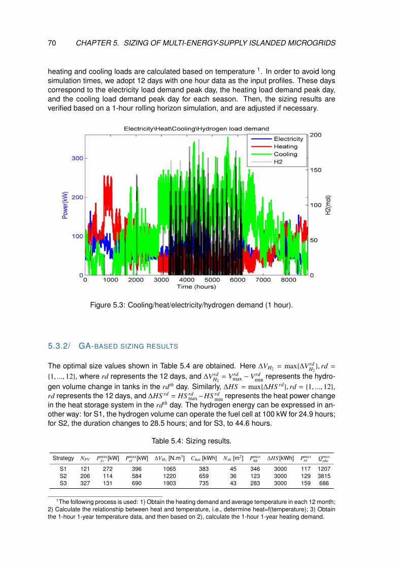
70 CHAPTER 5. SIZING OF MULTI-ENERGY-SUPPLY ISLANDED MICROGRIDS
heating and cooling loads are calculated based on temperature 1. In order to avoid longsimulation times, we adopt 12 days with one hour data as the input profiles. These dayscorrespond to the electricity load demand peak day, the heating load demand peak day,and the cooling load demand peak day for each season. Then, the sizing results areverified based on a 1-hour rolling horizon simulation, and are adjusted if necessary.
Figure 5.3: Cooling/heat/electricity/hydrogen demand (1 hour).
5.3.2/ GA-BASED SIZING RESULTS
The optimal size values shown in Table 5.4 are obtained. Here ∆VH2 = max{∆VrdH2}, rd =
{1, ..., 12}, where rd represents the 12 days, and ∆VrdH2
= Vrdmax − Vrd
min represents the hydro-gen volume change in tanks in the rdth day. Similarly, ∆HS = max{∆HS rd}, rd = {1, ..., 12},rd represents the 12 days, and ∆HS rd = HS rd
max−HS rdmin represents the heat power change
in the heat storage system in the rdth day. The hydrogen energy can be expressed in an-other way: for S1, the hydrogen volume can operate the fuel cell at 100 kW for 24.9 hours;for S2, the duration changes to 28.5 hours; and for S3, to 44.6 hours.
Table 5.4: Sizing results.
Strategy NPV Pmaxf c [kW] Pmax
el [kW] ∆VH2 [N.m3] Cbat [kWh] Nsh [m2] Pmaxhb ∆HS [kWh] Pmax
ac Qmaxahc
S1 121 272 396 1065 383 45 346 3000 117 1207S2 206 114 584 1220 659 36 123 3000 129 3815S3 327 131 690 1903 735 43 283 3000 159 686
1The following process is used: 1) Obtain the heating demand and average temperature in each 12 month;2) Calculate the relationship between heat and temperature, i.e., determine heat=f(temperature); 3) Obtainthe 1-hour 1-year temperature data, and then based on 2), calculate the 1-hour 1-year heating demand.
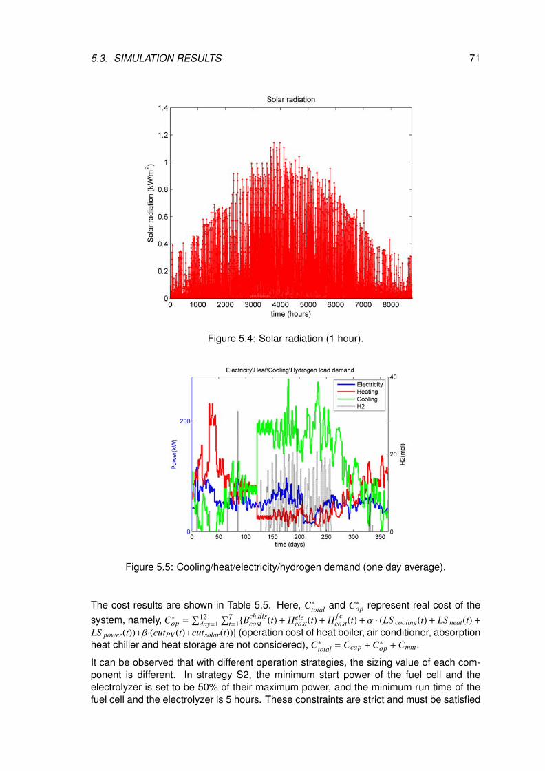
5.3. SIMULATION RESULTS 71
Figure 5.4: Solar radiation (1 hour).
Figure 5.5: Cooling/heat/electricity/hydrogen demand (one day average).
The cost results are shown in Table 5.5. Here, C∗total and C∗op represent real cost of thesystem, namely, C∗op =
∑12day=1
∑Tt=1{B
ch,discost (t) + Hele
cost(t) + H f ccost(t) + α · (LS cooling(t) + LS heat(t) +
LS power(t))+β·(cutPV (t)+cutsolar(t))} (operation cost of heat boiler, air conditioner, absorptionheat chiller and heat storage are not considered), C∗total = Ccap + C∗op + Cmnt.
It can be observed that with different operation strategies, the sizing value of each com-ponent is different. In strategy S2, the minimum start power of the fuel cell and theelectrolyzer is set to be 50% of their maximum power, and the minimum run time of thefuel cell and the electrolyzer is 5 hours. These constraints are strict and must be satisfied
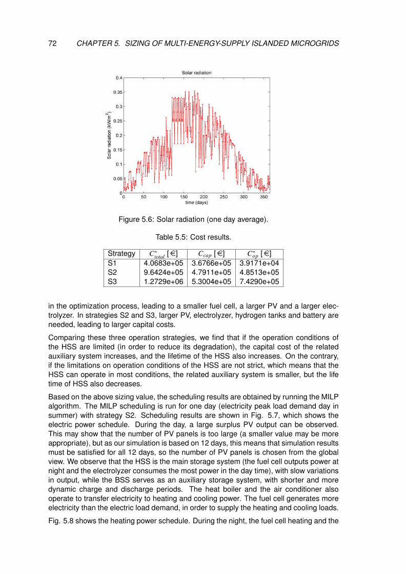
72 CHAPTER 5. SIZING OF MULTI-ENERGY-SUPPLY ISLANDED MICROGRIDS
Figure 5.6: Solar radiation (one day average).
Table 5.5: Cost results.
Strategy C∗total [e] Ccap [e] C∗op [e]S1 4.0683e+05 3.6766e+05 3.9171e+04S2 9.6424e+05 4.7911e+05 4.8513e+05S3 1.2729e+06 5.3004e+05 7.4290e+05
in the optimization process, leading to a smaller fuel cell, a larger PV and a larger elec-trolyzer. In strategies S2 and S3, larger PV, electrolyzer, hydrogen tanks and battery areneeded, leading to larger capital costs.
Comparing these three operation strategies, we find that if the operation conditions ofthe HSS are limited (in order to reduce its degradation), the capital cost of the relatedauxiliary system increases, and the lifetime of the HSS also increases. On the contrary,if the limitations on operation conditions of the HSS are not strict, which means that theHSS can operate in most conditions, the related auxiliary system is smaller, but the lifetime of HSS also decreases.
Based on the above sizing value, the scheduling results are obtained by running the MILPalgorithm. The MILP scheduling is run for one day (electricity peak load demand day insummer) with strategy S2. Scheduling results are shown in Fig. 5.7, which shows theelectric power schedule. During the day, a large surplus PV output can be observed.This may show that the number of PV panels is too large (a smaller value may be moreappropriate), but as our simulation is based on 12 days, this means that simulation resultsmust be satisfied for all 12 days, so the number of PV panels is chosen from the globalview. We observe that the HSS is the main storage system (the fuel cell outputs power atnight and the electrolyzer consumes the most power in the day time), with slow variationsin output, while the BSS serves as an auxiliary storage system, with shorter and moredynamic charge and discharge periods. The heat boiler and the air conditioner alsooperate to transfer electricity to heating and cooling power. The fuel cell generates moreelectricity than the electric load demand, in order to supply the heating and cooling loads.
Fig. 5.8 shows the heating power schedule. During the night, the fuel cell heating and the
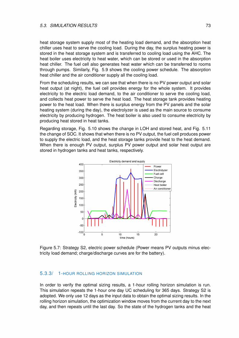
5.3. SIMULATION RESULTS 73
heat storage system supply most of the heating load demand, and the absorption heatchiller uses heat to serve the cooling load. During the day, the surplus heating power isstored in the heat storage system and is transferred to cooling load using the AHC. Theheat boiler uses electricity to heat water, which can be stored or used in the absorptionheat chiller. The fuel cell also generates heat water which can be transferred to roomsthrough pumps. Similarly, Fig. 5.9 shows the cooling power schedule. The absorptionheat chiller and the air conditioner supply all the cooling load.
From the scheduling results, we can see that when there is no PV power output and solarheat output (at night), the fuel cell provides energy for the whole system. It provideselectricity to the electric load demand, to the air conditioner to serve the cooling load,and collects heat power to serve the heat load. The heat storage tank provides heatingpower to the heat load. When there is surplus energy from the PV panels and the solarheating system (during the day), the electrolyzer is used as the main source to consumeelectricity by producing hydrogen. The heat boiler is also used to consume electricity byproducing heat stored in heat tanks.
Regarding storage, Fig. 5.10 shows the change in LOH and stored heat, and Fig. 5.11the change of SOC. It shows that when there is no PV output, the fuel cell produces powerto supply the electric load, and the heat storage tanks provide heat to the heat demand.When there is enough PV output, surplus PV power output and solar heat output arestored in hydrogen tanks and heat tanks, respectively.
Figure 5.7: Strategy S2, electric power schedule (Power means PV outputs minus elec-tricity load demand; charge/discharge curves are for the battery).
5.3.3/ 1-HOUR ROLLING HORIZON SIMULATION
In order to verify the optimal sizing results, a 1-hour rolling horizon simulation is run.This simulation repeats the 1-hour one day UC scheduling for 365 days. Strategy S2 isadopted. We only use 12 days as the input data to obtain the optimal sizing results. In therolling horizon simulation, the optimization window moves from the current day to the nextday, and then repeats until the last day. So the state of the hydrogen tanks and the heat
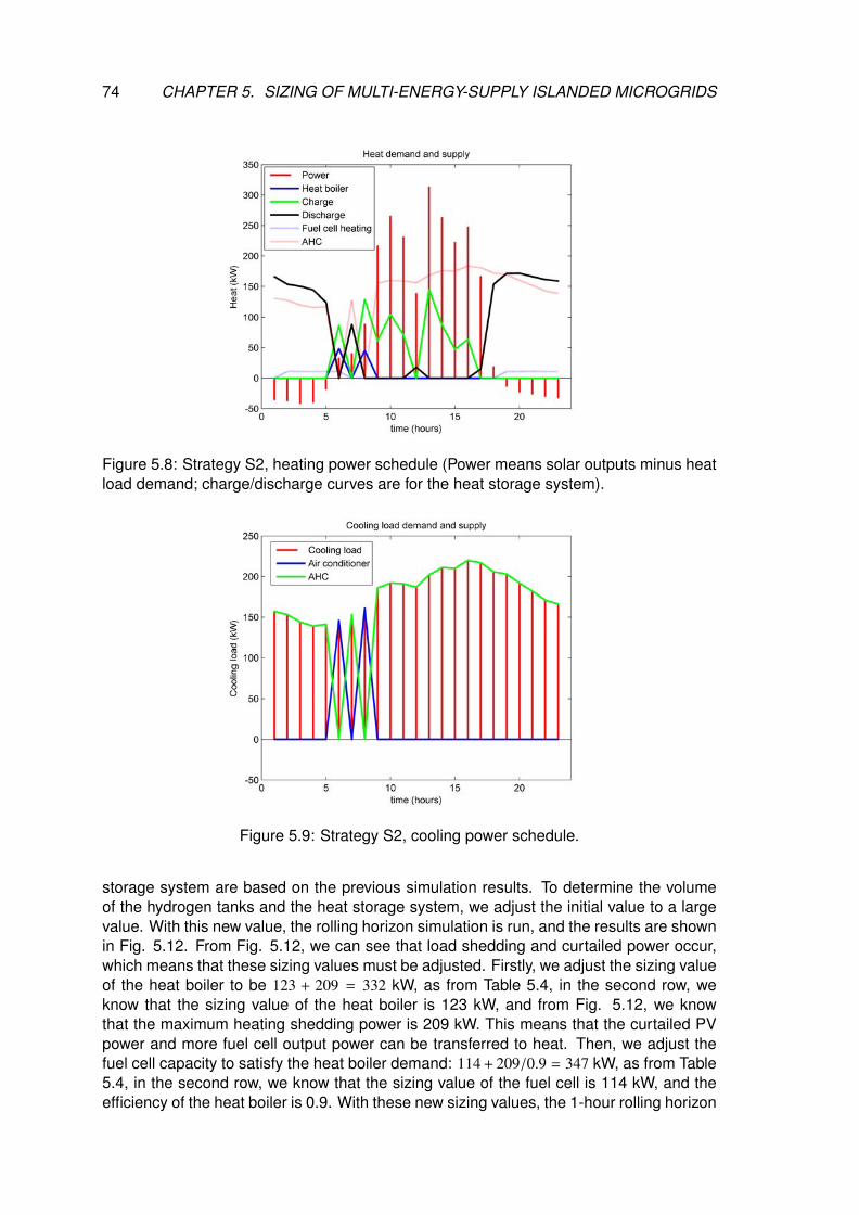
74 CHAPTER 5. SIZING OF MULTI-ENERGY-SUPPLY ISLANDED MICROGRIDS
Figure 5.8: Strategy S2, heating power schedule (Power means solar outputs minus heatload demand; charge/discharge curves are for the heat storage system).
Figure 5.9: Strategy S2, cooling power schedule.
storage system are based on the previous simulation results. To determine the volumeof the hydrogen tanks and the heat storage system, we adjust the initial value to a largevalue. With this new value, the rolling horizon simulation is run, and the results are shownin Fig. 5.12. From Fig. 5.12, we can see that load shedding and curtailed power occur,which means that these sizing values must be adjusted. Firstly, we adjust the sizing valueof the heat boiler to be 123 + 209 = 332 kW, as from Table 5.4, in the second row, weknow that the sizing value of the heat boiler is 123 kW, and from Fig. 5.12, we knowthat the maximum heating shedding power is 209 kW. This means that the curtailed PVpower and more fuel cell output power can be transferred to heat. Then, we adjust thefuel cell capacity to satisfy the heat boiler demand: 114 + 209/0.9 = 347 kW, as from Table5.4, in the second row, we know that the sizing value of the fuel cell is 114 kW, and theefficiency of the heat boiler is 0.9. With these new sizing values, the 1-hour rolling horizon
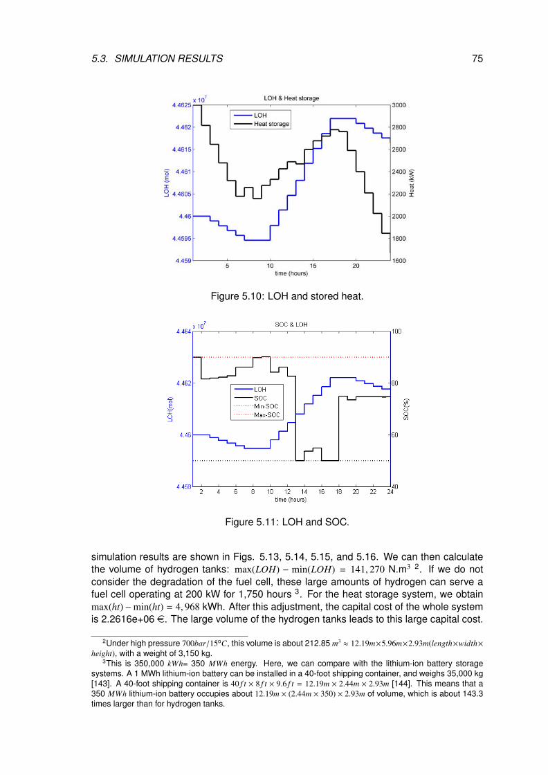
5.3. SIMULATION RESULTS 75
Figure 5.10: LOH and stored heat.
Figure 5.11: LOH and SOC.
simulation results are shown in Figs. 5.13, 5.14, 5.15, and 5.16. We can then calculatethe volume of hydrogen tanks: max(LOH) − min(LOH) = 141, 270 N.m3 2. If we do notconsider the degradation of the fuel cell, these large amounts of hydrogen can serve afuel cell operating at 200 kW for 1,750 hours 3. For the heat storage system, we obtainmax(ht)−min(ht) = 4, 968 kWh. After this adjustment, the capital cost of the whole systemis 2.2616e+06 e. The large volume of the hydrogen tanks leads to this large capital cost.
2Under high pressure 700bar/15oC, this volume is about 212.85 m3 ≈ 12.19m×5.96m×2.93m(length×width×height), with a weight of 3,150 kg.
3This is 350,000 kWh= 350 MWh energy. Here, we can compare with the lithium-ion battery storagesystems. A 1 MWh lithium-ion battery can be installed in a 40-foot shipping container, and weighs 35,000 kg[143]. A 40-foot shipping container is 40 f t × 8 f t × 9.6 f t = 12.19m × 2.44m × 2.93m [144]. This means that a350 MWh lithium-ion battery occupies about 12.19m × (2.44m × 350) × 2.93m of volume, which is about 143.3times larger than for hydrogen tanks.
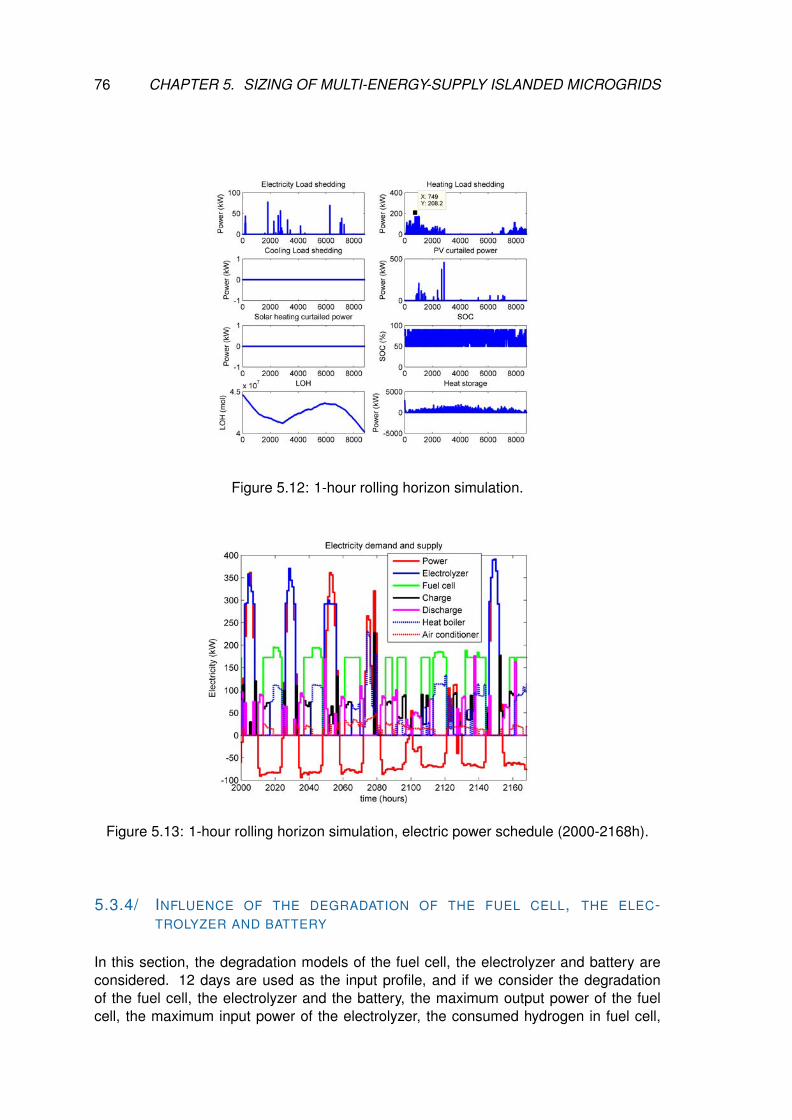
76 CHAPTER 5. SIZING OF MULTI-ENERGY-SUPPLY ISLANDED MICROGRIDS
Figure 5.12: 1-hour rolling horizon simulation.
Figure 5.13: 1-hour rolling horizon simulation, electric power schedule (2000-2168h).
5.3.4/ INFLUENCE OF THE DEGRADATION OF THE FUEL CELL, THE ELEC-TROLYZER AND BATTERY
In this section, the degradation models of the fuel cell, the electrolyzer and battery areconsidered. 12 days are used as the input profile, and if we consider the degradationof the fuel cell, the electrolyzer and the battery, the maximum output power of the fuelcell, the maximum input power of the electrolyzer, the consumed hydrogen in fuel cell,
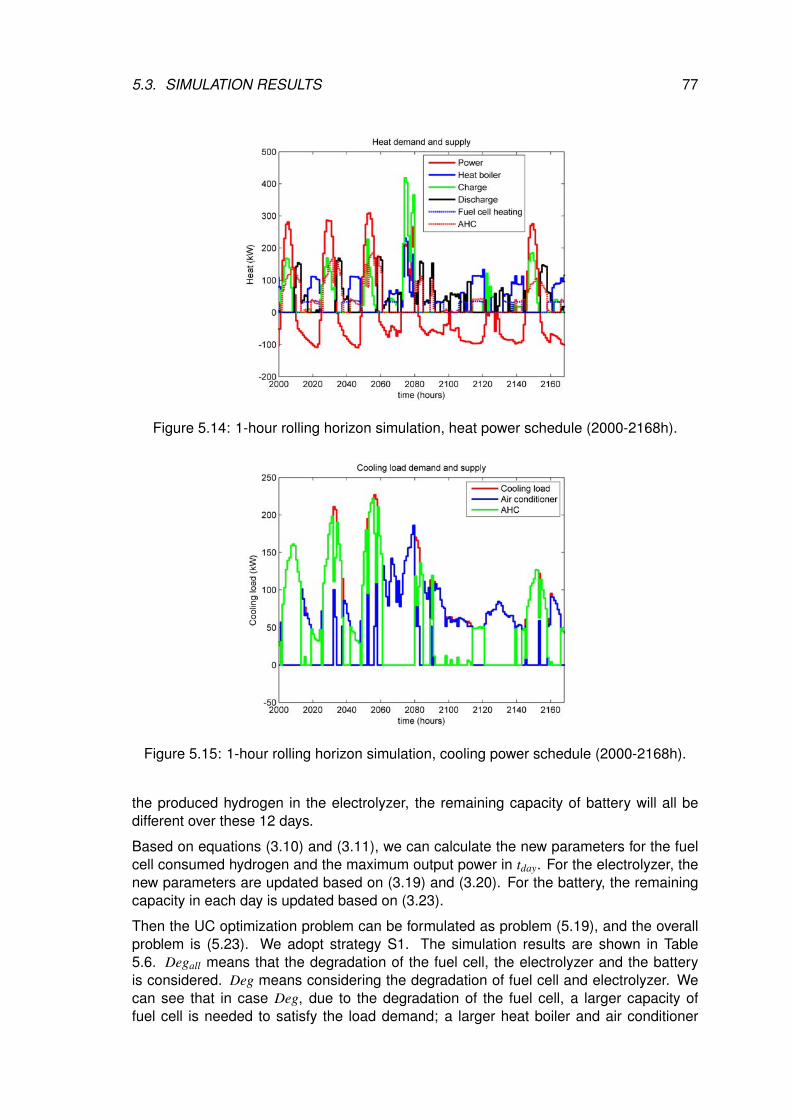
5.3. SIMULATION RESULTS 77
Figure 5.14: 1-hour rolling horizon simulation, heat power schedule (2000-2168h).
Figure 5.15: 1-hour rolling horizon simulation, cooling power schedule (2000-2168h).
the produced hydrogen in the electrolyzer, the remaining capacity of battery will all bedifferent over these 12 days.
Based on equations (3.10) and (3.11), we can calculate the new parameters for the fuelcell consumed hydrogen and the maximum output power in tday. For the electrolyzer, thenew parameters are updated based on (3.19) and (3.20). For the battery, the remainingcapacity in each day is updated based on (3.23).
Then the UC optimization problem can be formulated as problem (5.19), and the overallproblem is (5.23). We adopt strategy S1. The simulation results are shown in Table5.6. Degall means that the degradation of the fuel cell, the electrolyzer and the batteryis considered. Deg means considering the degradation of fuel cell and electrolyzer. Wecan see that in case Deg, due to the degradation of the fuel cell, a larger capacity offuel cell is needed to satisfy the load demand; a larger heat boiler and air conditioner
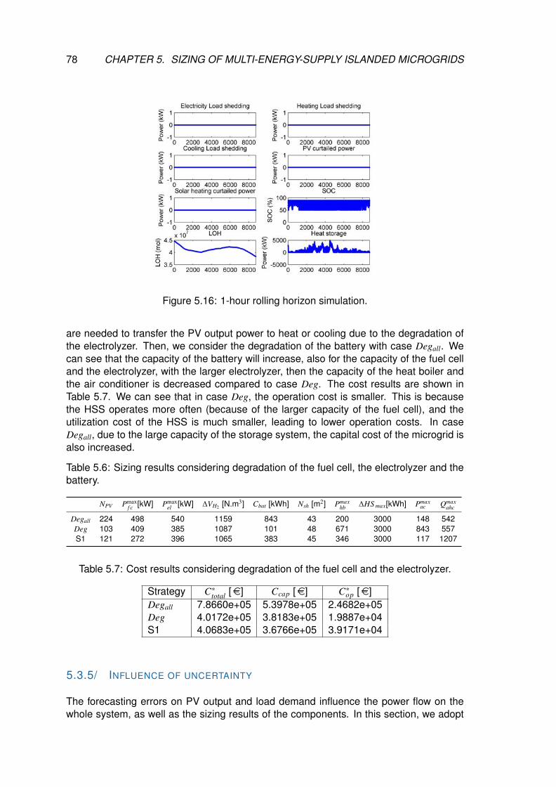
78 CHAPTER 5. SIZING OF MULTI-ENERGY-SUPPLY ISLANDED MICROGRIDS
Figure 5.16: 1-hour rolling horizon simulation.
are needed to transfer the PV output power to heat or cooling due to the degradation ofthe electrolyzer. Then, we consider the degradation of the battery with case Degall. Wecan see that the capacity of the battery will increase, also for the capacity of the fuel celland the electrolyzer, with the larger electrolyzer, then the capacity of the heat boiler andthe air conditioner is decreased compared to case Deg. The cost results are shown inTable 5.7. We can see that in case Deg, the operation cost is smaller. This is becausethe HSS operates more often (because of the larger capacity of the fuel cell), and theutilization cost of the HSS is much smaller, leading to lower operation costs. In caseDegall, due to the large capacity of the storage system, the capital cost of the microgrid isalso increased.
Table 5.6: Sizing results considering degradation of the fuel cell, the electrolyzer and thebattery.
NPV Pmaxf c [kW] Pmax
el [kW] ∆VH2 [N.m3] Cbat [kWh] Nsh [m2] Pmaxhb ∆HS max[kWh] Pmax
ac Qmaxahc
Degall 224 498 540 1159 843 43 200 3000 148 542Deg 103 409 385 1087 101 48 671 3000 843 557S1 121 272 396 1065 383 45 346 3000 117 1207
Table 5.7: Cost results considering degradation of the fuel cell and the electrolyzer.
Strategy C∗total [e] Ccap [e] C∗op [e]Degall 7.8660e+05 5.3978e+05 2.4682e+05Deg 4.0172e+05 3.8183e+05 1.9887e+04S1 4.0683e+05 3.6766e+05 3.9171e+04
5.3.5/ INFLUENCE OF UNCERTAINTY
The forecasting errors on PV output and load demand influence the power flow on thewhole system, as well as the sizing results of the components. In this section, we adopt
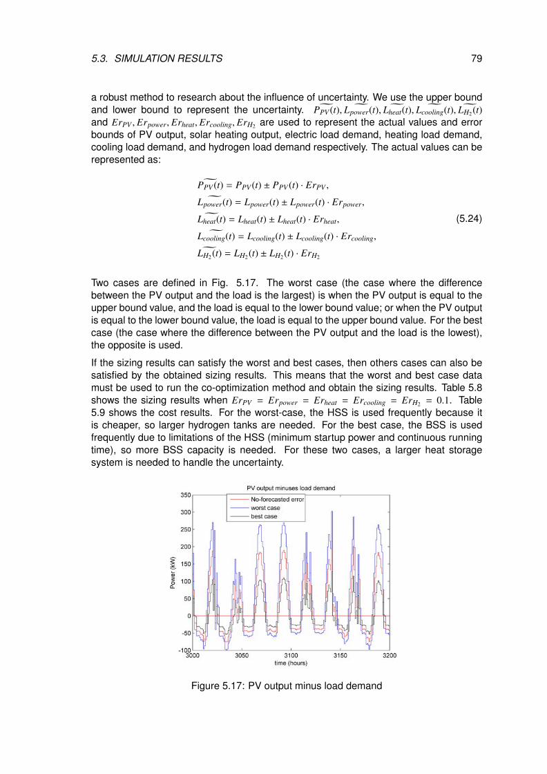
5.3. SIMULATION RESULTS 79
a robust method to research about the influence of uncertainty. We use the upper boundand lower bound to represent the uncertainty. ˜PPV (t), ˜Lpower(t), ˜Lheat(t), ˜Lcooling(t), ˜LH2(t)and ErPV , Erpower, Erheat, Ercooling, ErH2 are used to represent the actual values and errorbounds of PV output, solar heating output, electric load demand, heating load demand,cooling load demand, and hydrogen load demand respectively. The actual values can berepresented as:
˜PPV (t) = PPV (t) ± PPV (t) · ErPV ,˜Lpower(t) = Lpower(t) ± Lpower(t) · Erpower,˜Lheat(t) = Lheat(t) ± Lheat(t) · Erheat,˜Lcooling(t) = Lcooling(t) ± Lcooling(t) · Ercooling,˜LH2(t) = LH2(t) ± LH2(t) · ErH2
(5.24)
Two cases are defined in Fig. 5.17. The worst case (the case where the differencebetween the PV output and the load is the largest) is when the PV output is equal to theupper bound value, and the load is equal to the lower bound value; or when the PV outputis equal to the lower bound value, the load is equal to the upper bound value. For the bestcase (the case where the difference between the PV output and the load is the lowest),the opposite is used.
If the sizing results can satisfy the worst and best cases, then others cases can also besatisfied by the obtained sizing results. This means that the worst and best case datamust be used to run the co-optimization method and obtain the sizing results. Table 5.8shows the sizing results when ErPV = Erpower = Erheat = Ercooling = ErH2 = 0.1. Table5.9 shows the cost results. For the worst-case, the HSS is used frequently because itis cheaper, so larger hydrogen tanks are needed. For the best case, the BSS is usedfrequently due to limitations of the HSS (minimum startup power and continuous runningtime), so more BSS capacity is needed. For these two cases, a larger heat storagesystem is needed to handle the uncertainty.
Figure 5.17: PV output minus load demand
80 CHAPTER 5. SIZING OF MULTI-ENERGY-SUPPLY ISLANDED MICROGRIDS
Table 5.8: Sizing results considering uncertainty. The worst case is defined as the casewhere the difference between PV output and load is the largest, and the lowest for thebest case.
Strategy NPV Pmaxf c [kW] Pmax
el [kW] ∆VH2 [N.m3] Cbat [kWh] Nsh [m2] Pmaxhb ∆HS max[kWh] Pmax
ac Qmaxahc
Worst case 109 169 307 1199 437 105 323 9072 81 531Best case 107 191 247 952 652 124 324 8219 337 2728
S1 121 272 396 1065 383 45 346 3000 117 1207
Table 5.9: Cost results considering uncertainty.
Strategy C∗total [e] Ccap [e] C∗op [e]Worst case 3.9060e+05 3.7248e+05 1.8123e+04Best case 4.5288e+05 4.2616e+05 2.6729e+04S1 4.0683e+05 3.6766e+05 3.9171e+04
5.4/ CONCLUSION
In this chapter, we introduced a co-optimization method to size the components of arenewable energy based stand-alone microgrid which combines cooling, heat, electricpower and hydrogen loads. The UC optimization method was used for defining the op-eration strategy, which aims at minimizing the operation cost through an MILP algorithm.A GA was used to compute the sizing value of each component, aiming to minimize thetotal cost. Three operation strategies were compared, which showed that sizing valuesare different with different strategies. Then a 1-hour rolling horizon simulation was usedto adjust the sizing values of several components. The degradation of the fuel cell, theelectrolyzer and the battery was also considered and showed that the sizing values ofthe fuel cell and the battery increases when considering the degradation. Uncertaintyon PV output and load demand was addressed using robust optimization, and resultsshowed that larger volumes of hydrogen tanks and heat storage are needed to tacklethese uncertainty factors. This co-optimization method is useful to size complex islandedmicrogrids, and results show that the optimal size value and operation algorithms arecapable of scheduling multiple components and managing flows from different natures(heat/cooling, electricity and hydrogen).
The above two chapters are discussing islanded microgrids, but do not consider the influ-ence of the utility grid. Then, in next chapter, grid-connected microgrids are considered,and the sizing and operation of grid-connected microgrids are presented.
6SIZING OF GRID-CONNECTED
MULTI-ENERGY-SUPPLY MICROGRIDS
This chapter is based on the author’s published paper: Li Bei, Robin Roche,Damien Paire, and Abdellatif Miraoui. “Optimal sizing of distributed generation ingas/electricity/heat supply networks.” Energy 151 (2018): 675-688.
Today’s energy supply systems are large transmission networks, such as the electric-ity network and gas supply network. Normally, these energy supply networks are
planned separately. However, load demands are often with several types of energy in thesame time step. For example, when people use gas to cook, people also need electricityto serve electronic devices, and heat energy to heat the room. When these large energysupply systems co-operate together, it can improve the efficiency of the whole energysupply system, because co-operating can make the whole system operate in an optimalstate, and in the same time, ensure the power balance of different energy supplies.
On the other hand, at each interconnection node, different types of energy can be con-verted to each other through power devices. For example, fuel cells can be used to con-vert H2 to electricity, electrolyzers can be used to convert electricity to H2, gas turbinescan be used to convert gas to heat, etc. At each node, renewable energy can also beconnected, such as with photovoltaic (PV) panels and wind turbines. In this chapter, thefocus is on the following problem: how to determine the capacity of these power devicesand renewable energy sources at each interconnection node, based on the given hybridenergy network configuration?
In this work, a modified 13-node network is considered (the electricity network is theIEEE 13-node network [145], and the gas and heating networks are assumed to havethe same structure as the electricity network, as shown in Fig. 6.1, and three types ofgas/electricity/heat load demands are served. In this figure, HS represents a hydrogenstorage system (fuel cell + electrolyzer + tanks), which has several advantages, such asa high storage capacity, and a high energy per unit of volume [5]; CHP is a combinedheat and power device; ETH is a device that converts electricity to heat, for example, aheat boiler; GTH is a device that converts gas to heat, for example, a gas boiler heater.Black lines represent the gas supply system, blue lines are the electricity supply system,red lines are the heat supply system.
At each node, the devices and load demands can be formed as an MG or an energyhub (EH). In [146], authors design a combined cooling/heat/power and hydrogen MGsystem, and present a combined GA and MILP method to size such MES MG. GA isused to search for the sizing values, MILP is used to control the operation of MG. In
81
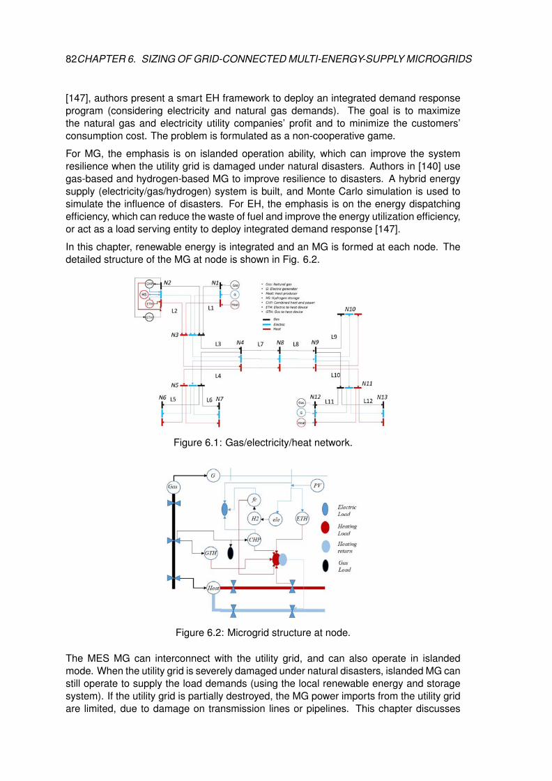
82CHAPTER 6. SIZING OF GRID-CONNECTED MULTI-ENERGY-SUPPLY MICROGRIDS
[147], authors present a smart EH framework to deploy an integrated demand responseprogram (considering electricity and natural gas demands). The goal is to maximizethe natural gas and electricity utility companies’ profit and to minimize the customers’consumption cost. The problem is formulated as a non-cooperative game.
For MG, the emphasis is on islanded operation ability, which can improve the systemresilience when the utility grid is damaged under natural disasters. Authors in [140] usegas-based and hydrogen-based MG to improve resilience to disasters. A hybrid energysupply (electricity/gas/hydrogen) system is built, and Monte Carlo simulation is used tosimulate the influence of disasters. For EH, the emphasis is on the energy dispatchingefficiency, which can reduce the waste of fuel and improve the energy utilization efficiency,or act as a load serving entity to deploy integrated demand response [147].
In this chapter, renewable energy is integrated and an MG is formed at each node. Thedetailed structure of the MG at node is shown in Fig. 6.2.
Figure 6.1: Gas/electricity/heat network.
Figure 6.2: Microgrid structure at node.
The MES MG can interconnect with the utility grid, and can also operate in islandedmode. When the utility grid is severely damaged under natural disasters, islanded MG canstill operate to supply the load demands (using the local renewable energy and storagesystem). If the utility grid is partially destroyed, the MG power imports from the utility gridare limited, due to damage on transmission lines or pipelines. This chapter discusses
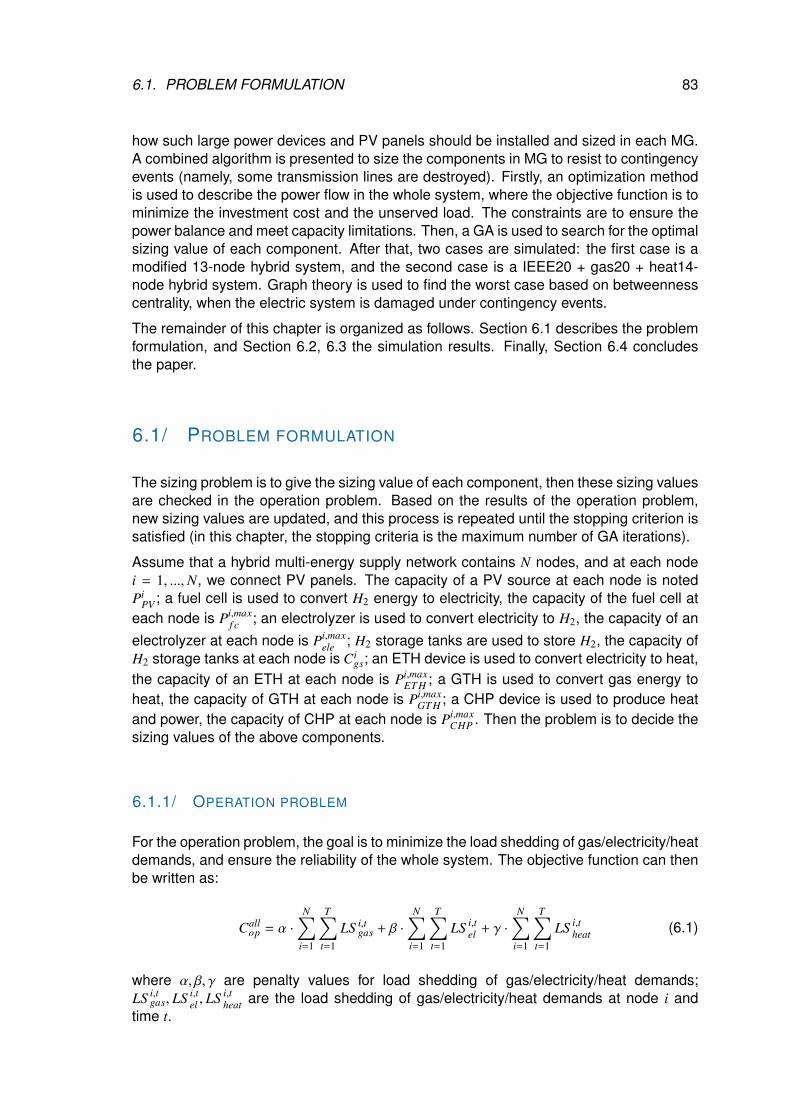
6.1. PROBLEM FORMULATION 83
how such large power devices and PV panels should be installed and sized in each MG.A combined algorithm is presented to size the components in MG to resist to contingencyevents (namely, some transmission lines are destroyed). Firstly, an optimization methodis used to describe the power flow in the whole system, where the objective function is tominimize the investment cost and the unserved load. The constraints are to ensure thepower balance and meet capacity limitations. Then, a GA is used to search for the optimalsizing value of each component. After that, two cases are simulated: the first case is amodified 13-node hybrid system, and the second case is a IEEE20 + gas20 + heat14-node hybrid system. Graph theory is used to find the worst case based on betweennesscentrality, when the electric system is damaged under contingency events.
The remainder of this chapter is organized as follows. Section 6.1 describes the problemformulation, and Section 6.2, 6.3 the simulation results. Finally, Section 6.4 concludesthe paper.
6.1/ PROBLEM FORMULATION
The sizing problem is to give the sizing value of each component, then these sizing valuesare checked in the operation problem. Based on the results of the operation problem,new sizing values are updated, and this process is repeated until the stopping criterion issatisfied (in this chapter, the stopping criteria is the maximum number of GA iterations).
Assume that a hybrid multi-energy supply network contains N nodes, and at each nodei = 1, ...,N, we connect PV panels. The capacity of a PV source at each node is notedPi
PV ; a fuel cell is used to convert H2 energy to electricity, the capacity of the fuel cell ateach node is Pi,max
f c ; an electrolyzer is used to convert electricity to H2, the capacity of anelectrolyzer at each node is Pi,max
ele ; H2 storage tanks are used to store H2, the capacity ofH2 storage tanks at each node is Ci
gs; an ETH device is used to convert electricity to heat,the capacity of an ETH at each node is Pi,max
ET H ; a GTH is used to convert gas energy toheat, the capacity of GTH at each node is Pi,max
GT H ; a CHP device is used to produce heatand power, the capacity of CHP at each node is Pi,max
CHP . Then the problem is to decide thesizing values of the above components.
6.1.1/ OPERATION PROBLEM
For the operation problem, the goal is to minimize the load shedding of gas/electricity/heatdemands, and ensure the reliability of the whole system. The objective function can thenbe written as:
Callop = α ·
N∑i=1
T∑t=1
LS i,tgas + β ·
N∑i=1
T∑t=1
LS i,tel + γ ·
N∑i=1
T∑t=1
LS i,theat (6.1)
where α, β, γ are penalty values for load shedding of gas/electricity/heat demands;LS i,t
gas, LS i,tel , LS i,t
heat are the load shedding of gas/electricity/heat demands at node i andtime t.
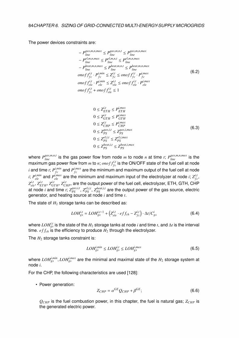
84CHAPTER 6. SIZING OF GRID-CONNECTED MULTI-ENERGY-SUPPLY MICROGRIDS
The power devices constraints are:
− Pgas,m,n,maxline ≤ Pgas,m,n,t
line ≤ Pgas,m,n,maxline
− Pel,m,n,maxline ≤ Pel,m,n,t
line ≤ Pel,m,n,maxline
− Pheat,m,n,maxline ≤ Pheat,m,n,t
line ≤ Pheat,m,n,maxline
ono f f i,tf c · P
i,minf c ≤ Zi,t
f c ≤ ono f f i,tf c · P
i,maxf c
ono f f i,tele · P
i,minele ≤ Zi,t
ele ≤ ono f f i,tele · P
i,maxele
ono f f i,tf c + ono f f i,t
ele ≤ 1
(6.2)
0 ≤ Zi,tET H ≤ Pi,max
ET H
0 ≤ Zi,tGT H ≤ Pi,max
GT H
0 ≤ Zi,tCHP ≤ Pi,max
CHP
0 ≤ Zgas,i,tPS ≤ Zgas,i,max
PS
0 ≤ Zel,i,tPS ≤ Zel,i,max
PS
0 ≤ Zheat,i,tPS ≤ Zheat,i,max
PS
(6.3)
where Pgas,m,n,tline is the gas power flow from node m to node n at time t; Pgas,m,n,max
line is themaximum gas power flow from m to n; ono f f i,t
f c is the ON/OFF state of the fuel cell at nodei and time t; Pi,min
f c and Pi,maxf c are the minimum and maximum output of the fuel cell at node
i; Pi,minele and Pi,max
ele are the minimum and maximum input of the electrolyzer at node i; Zi,tf c,
Zi,tele, Zi,t
ET H, Zi,tGT H, Zi,t
CHP, are the output power of the fuel cell, electrolyzer, ETH, GTH, CHPat node i and time t; Zgas,i,t
PS , Zel,i,tPS , Zheat,i,t
PS are the output power of the gas source, electricgenerator, and heating source at node i and time t.
The state of H2 storage tanks can be described as:
LOHi,tgs = LOHi,t−1
gs +(Zi,t
ele · e f fch − Zi,tf c
)· ∆t/Ci
gs (6.4)
where LOHi,tgs is the state of the H2 storage tanks at node i and time t, and ∆t is the interval
time. e f fch is the efficiency to produce H2 through the electrolyzer.
The H2 storage tanks constraint is:
LOHi,mings ≤ LOHi,t
gs ≤ LOHi,maxgs (6.5)
where LOHi,mings , LOHi,max
gs are the minimal and maximal state of the H2 storage system atnode i.
For the CHP, the following characteristics are used [128]:
• Power generation:ZCHP = αGEQCHP + βGE; (6.6)
QCHP is the fuel combustion power, in this chapter, the fuel is natural gas; ZCHP isthe generated electric power.
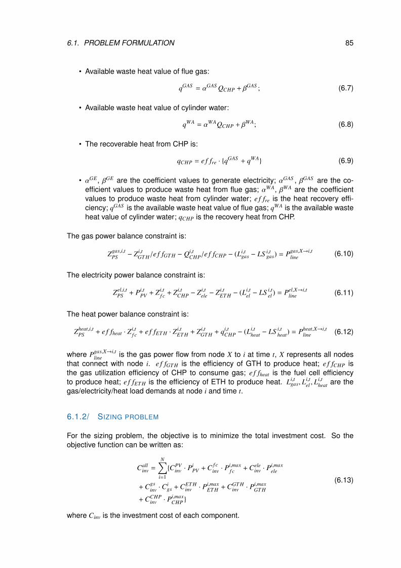
6.1. PROBLEM FORMULATION 85
• Available waste heat value of flue gas:
qGAS = αGAS QCHP + βGAS ; (6.7)
• Available waste heat value of cylinder water:
qWA = αWAQCHP + βWA; (6.8)
• The recoverable heat from CHP is:
qCHP = e f fre · {qGAS + qWA} (6.9)
• αGE, βGE are the coefficient values to generate electricity; αGAS , βGAS are the co-efficient values to produce waste heat from flue gas; αWA, βWA are the coefficientvalues to produce waste heat from cylinder water; e f fre is the heat recovery effi-ciency; qGAS is the available waste heat value of flue gas; qWA is the available wasteheat value of cylinder water; qCHP is the recovery heat from CHP.
The gas power balance constraint is:
Zgas,i,tPS − Zi,t
GT H/e f fGT H − Qi,tCHP/e f fCHP − (Li,t
gas − LS i,tgas) = Pgas,X→i,t
line (6.10)
The electricity power balance constraint is:
Zel,i,tPS + Pi,t
PV + Zi,tf c + Zi,t
CHP − Zi,tele − Zi,t
ET H − (Li,tel − LS i,t
el ) = Pel,X→i,tline (6.11)
The heat power balance constraint is:
Zheat,i,tPS + e f fheat · Z
i,tf c + e f fET H · Z
i,tET H + Zi,t
GT H + qi,tCHP − (Li,t
heat − LS i,theat) = Pheat,X→i,t
line (6.12)
where Pgas,X→i,tline is the gas power flow from node X to i at time t, X represents all nodes
that connect with node i. e f fGT H is the efficiency of GTH to produce heat; e f fCHP isthe gas utilization efficiency of CHP to consume gas; e f fheat is the fuel cell efficiencyto produce heat; e f fET H is the efficiency of ETH to produce heat. Li,t
gas, Li,tel , L
i,theat are the
gas/electricity/heat load demands at node i and time t.
6.1.2/ SIZING PROBLEM
For the sizing problem, the objective is to minimize the total investment cost. So theobjective function can be written as:
Callinv =
N∑i=1
{CPVinv · P
iPV + C f c
inv · Pi,maxf c + Cele
inv · Pi,maxele
+ Cgsinv ·C
igs + CET H
inv · Pi,maxET H + CGT H
inv · Pi,maxGT H
+ CCHPinv · Pi,max
CHP }
(6.13)
where Cinv is the investment cost of each component.

86CHAPTER 6. SIZING OF GRID-CONNECTED MULTI-ENERGY-SUPPLY MICROGRIDS
U is used to represent the set of the sizing problem variables, namely, U ={Pi
PV , Pi,maxf c , Pi,max
ele ,Cigs, P
i,maxET H , P
i,maxGT H , P
i,maxCHP
}, i = 1, ...,N. S represents the set of the opera-
tion problem variables. At last, the sizing problem of the hybrid gas/electricity/heat systemcan be written as:
minU
{Call
inv + minU∗,S
{Call
op
}}s.t. (6.2), (6.3), (6.4), (6.5), (6.6), (6.7), (6.8), (6.9), (6.10), (6.11), (6.12)
(6.14)
6.1.3/ CONSIDERING THE CONTINGENCY EVENTS
In large nodes hybrid network, contingency events must be considered. In this section,the influence of contingency events on the sizing results are developed. A large numberof contingency events can be listed, and it is impossible to consider all cases. So a robustmethod can be used to find the worst case. The sizing problem can then be describedas:
minU
{Call
inv + mV
ax minU∗,S
{Call
op
}}s.t. (6.2), (6.3), (6.4), (6.5), (6.6), (6.7), (6.8), (6.9), (6.10), (6.11), (6.12)
(6.15)
where V represents the contingency events set.
Then the problem can be described as: search for the best sizing values U∗ from U, whichcan make the whole system operate with minimal costs, and at the same time, ensure thewhole system resists the worst contingency event.
For this two stage optimization problem, the column-and-constraint generation method[148] is used. In [149], authors use this method to solve a robust microgrid planningproblem. In [150], authors solve a distribution network planning problem to minimize thesystem damage against natural disasters.
For example, in [150], the problem can be summarized as follows:
minh∈Y
maxu∈U
minz∈f(h,u)
∑pld (6.16)
h ∈ Y is the hardening plans to resist to natural disasters; u ∈ U is the natural disastersscenarios; z ∈ f(h, u) is the disruption with feasible power flow decisions;
∑pld is the load
shedding.
Then the problem can be described as: search for the hardening plans h∗ from Y, whichcan make the whole system operate with minimal load shedding, and at the same time,ensure the whole system resists the worst natural disasters.
Load shedding of the distribution network after hardening lines and DG placement plan-ning (h) and disaster impact (u) can be formulated as: z = (p, q, v) ∈ f(h, u). Using anabstract form to describe this feasible set, we have:
f(h, u) = {z : Ah + Bu + Cz ≥ e} (6.17)
Problem 6.16 is a two stage robust optimization problem that can be transferred into twooptimization problems, namely, a master problem and a subproblem. The master problem
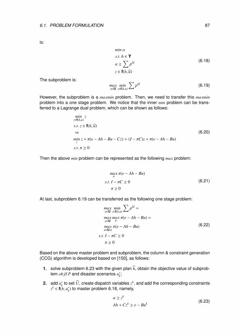
6.1. PROBLEM FORMULATION 87
is:
min α
s.t. h ∈ Y
α ≥∑
pld
z ∈ f(h, u)
(6.18)
The subproblem is:maxu∈U
minz∈f(h,u)
∑pld (6.19)
However, the subproblem is a maxmin problem. Then, we need to transfer this maxminproblem into a one stage problem. We notice that the inner min problem can be trans-ferred to a Lagrange dual problem, which can be shown as follows:
minz∈f(h,u)
z
s.t. z ∈ f(h, u)
⇒
minz
z + π(e − Ah − Bu −Cz) = (I − πC)z + π(e − Ah − Bu)
s.t. π ≥ 0
(6.20)
Then the above min problem can be represented as the following max problem:
maxπ
π(e − Ah − Bu)
s.t. I − πC ≥ 0
π ≥ 0
(6.21)
At last, subproblem 6.19 can be transferred as the following one stage problem:
maxu∈U
minz∈f(h,u)
∑pld =
maxu∈U
maxπ
π(e − Ah − Bu) =
maxu∈U,π
π(e − Ah − Bu)
s.t. I − πC ≥ 0
π ≥ 0
(6.22)
Based on the above master problem and subproblem, the column & constraint generation(CCG) algorithm is developed based on [150], as follows:
1. solve subproblem 6.23 with the given plan h, obtain the objective value of subprob-lem ob jS P and disaster scenarios u∗k;
2. add u∗k to set U, create dispatch variables zk, and add the corresponding constraintszk ∈ f(h, u∗k) to master problem 6.18, namely,
α ≥ zk
Ah + Czk ≥ e − Buk (6.23)

88CHAPTER 6. SIZING OF GRID-CONNECTED MULTI-ENERGY-SUPPLY MICROGRIDS
3. solve master problem 6.18, obtain the objective value of master problem ob jMP andupdate the planning plan h;
4. repeat this process until the gap between ob jMP and ob jS P is less than a smallvalue.
We can see that with the CCG algorithm, the uncertainty set is transferred based onLagrange dual problem, and two stage optimization is decomposed into a master and asubproblem.
In this chapter, the uncertainty set of disasters is described based on graph theory, anda two stage sizing problem is decomposed into a leader and a follower problem. A com-parison between the CCG method and the presented method is summarized in Tab. 6.1.
Table 6.1: Comparison between the CCG method and our method.
Method Disasters scenarios Two stage problem Running ComplexityCCG [150] Lagrange dual problem master & sub problem iteration repeat highProposed graph theory leader & follower problem iteration repeat medium
In our method, the worst case is obtained based on graph theory. For the large nodeshybrid network system, the relative importance of each node is ranked. The case wherethe most important node is destroyed under the contingency event, is the worst case. Therelative importance of each node in the graph is described using betweenness centrality[151] of the node:
CB(i) =∑
ni,nk,nl
nk → nl, ni
nk → nl(6.24)
where nk → nl, ni is 1 if the shortest path between nodes nk to nl goes through ni, and 0 ifnk to nl does not pass through ni.
Under the worst case, the new structure of the whole system can be obtained. Then thesizing problem (7.31) is solved based on this new structure, and new sizing values canbe obtained.
6.2/ SIMULATION RESULTS FOR CASE I
In this section, the modified 13-node case is tested. Three cases are compared. For theoperation problem, the time step is 1 hour, and time horizon is one day (24h).
6.2.1/ SYSTEM SETUP
The penalty values are arbitrarily chosen as α = β = γ = 1010 to make sure that thepenalty cost of load shedding is larger than that of the total investment cost. Investmentcosts are shown in Tab. 6.2. The cost parameters are adopted from [145, 142]. The modelis implemented in MATLAB and solved with YALMIP [152] and Gurobi. Simulations wererun on a computer with an Intel Xeon CPU [email protected].
Load demands (peak load) at each node are shown in Tab. 6.3. Source data is shown inTab. 6.4. The capacity of transportation lines is shown in Tab. 6.5, where the unit is MW.
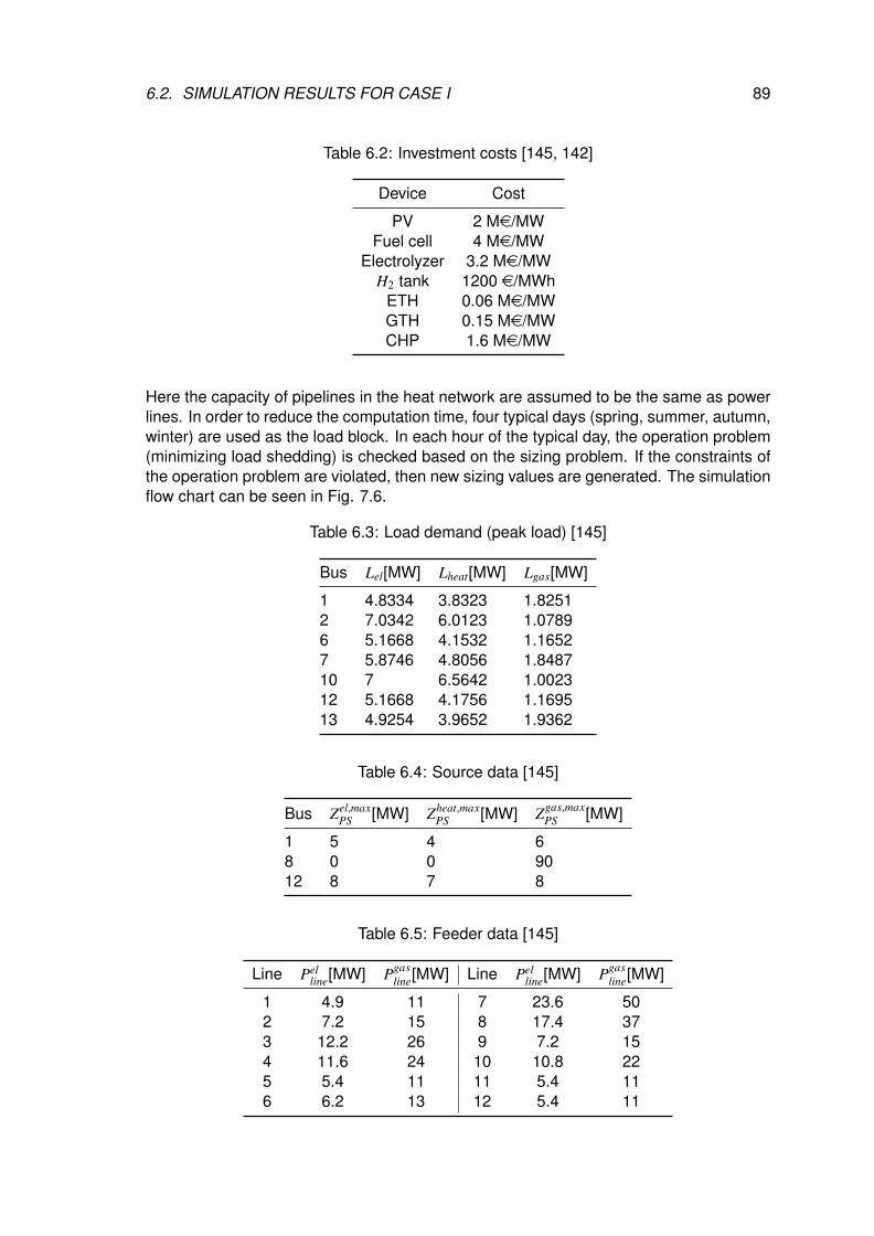
6.2. SIMULATION RESULTS FOR CASE I 89
Table 6.2: Investment costs [145, 142]
Device Cost
PV 2 Me/MWFuel cell 4 Me/MW
Electrolyzer 3.2 Me/MWH2 tank 1200 e/MWh
ETH 0.06 Me/MWGTH 0.15 Me/MWCHP 1.6 Me/MW
Here the capacity of pipelines in the heat network are assumed to be the same as powerlines. In order to reduce the computation time, four typical days (spring, summer, autumn,winter) are used as the load block. In each hour of the typical day, the operation problem(minimizing load shedding) is checked based on the sizing problem. If the constraints ofthe operation problem are violated, then new sizing values are generated. The simulationflow chart can be seen in Fig. 7.6.
Table 6.3: Load demand (peak load) [145]
Bus Lel[MW] Lheat[MW] Lgas[MW]
1 4.8334 3.8323 1.82512 7.0342 6.0123 1.07896 5.1668 4.1532 1.16527 5.8746 4.8056 1.848710 7 6.5642 1.002312 5.1668 4.1756 1.169513 4.9254 3.9652 1.9362
Table 6.4: Source data [145]
Bus Zel,maxPS [MW] Zheat,max
PS [MW] Zgas,maxPS [MW]
1 5 4 68 0 0 9012 8 7 8
Table 6.5: Feeder data [145]
Line Pelline[MW] Pgas
line[MW] Line Pelline[MW] Pgas
line[MW]
1 4.9 11 7 23.6 502 7.2 15 8 17.4 373 12.2 26 9 7.2 154 11.6 24 10 10.8 225 5.4 11 11 5.4 116 6.2 13 12 5.4 11
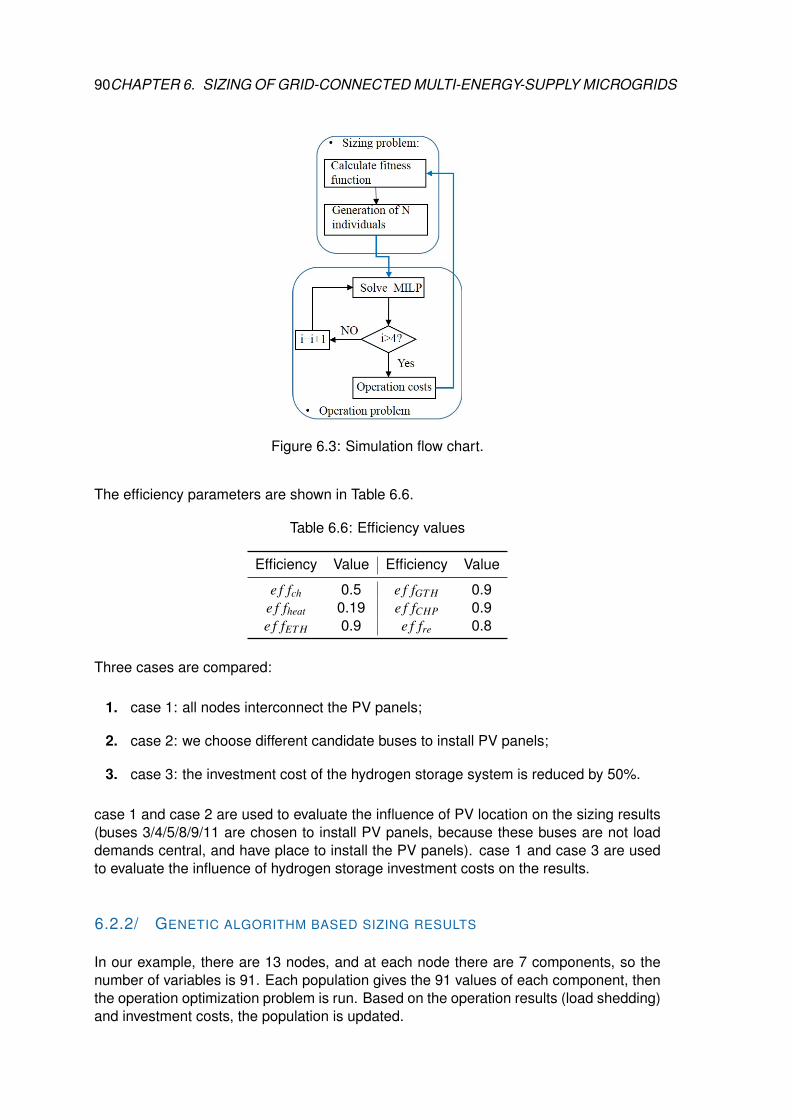
90CHAPTER 6. SIZING OF GRID-CONNECTED MULTI-ENERGY-SUPPLY MICROGRIDS
Figure 6.3: Simulation flow chart.
The efficiency parameters are shown in Table 6.6.
Table 6.6: Efficiency values
Efficiency Value Efficiency Value
e f fch 0.5 e f fGT H 0.9e f fheat 0.19 e f fCHP 0.9e f fET H 0.9 e f fre 0.8
Three cases are compared:
1. case 1: all nodes interconnect the PV panels;
2. case 2: we choose different candidate buses to install PV panels;
3. case 3: the investment cost of the hydrogen storage system is reduced by 50%.
case 1 and case 2 are used to evaluate the influence of PV location on the sizing results(buses 3/4/5/8/9/11 are chosen to install PV panels, because these buses are not loaddemands central, and have place to install the PV panels). case 1 and case 3 are usedto evaluate the influence of hydrogen storage investment costs on the results.
6.2.2/ GENETIC ALGORITHM BASED SIZING RESULTS
In our example, there are 13 nodes, and at each node there are 7 components, so thenumber of variables is 91. Each population gives the 91 values of each component, thenthe operation optimization problem is run. Based on the operation results (load shedding)and investment costs, the population is updated.
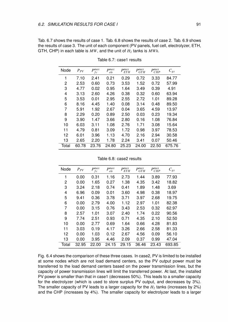
6.2. SIMULATION RESULTS FOR CASE I 91
Tab. 6.7 shows the results of case 1. Tab. 6.8 shows the results of case 2. Tab. 6.9 showsthe results of case 3. The unit of each component (PV panels, fuel cell, electrolyzer, ETH,GTH, CHP) in each table is MW, and the unit of H2 tanks is MWh.
Table 6.7: case1 results
Node PPV Pmaxf c Pmax
ele PmaxET H Pmax
GT H PmaxCHP Cgs
1 7.10 2.41 0.21 0.29 0.72 3.33 84.772 2.53 0.60 0.73 3.53 1.52 0.72 57.993 4.77 0.02 0.95 1.64 3.49 0.39 4.914 3.13 2.60 4.26 0.38 0.32 0.60 63.945 3.53 0.01 2.95 2.55 2.72 1.01 89.286 8.16 4.45 1.40 0.08 3.14 0.48 89.507 5.91 1.92 2.67 0.04 3.65 4.59 13.978 2.29 0.20 0.89 2.50 0.03 0.23 19.349 3.90 1.47 3.66 2.80 0.16 1.08 76.84
10 6.03 3.11 1.08 2.76 1.71 3.08 15.6411 4.79 0.81 3.09 1.72 0.98 3.97 78.5312 6.01 3.96 1.13 4.70 2.16 2.94 30.5813 2.65 2.20 1.78 2.24 3.41 0.07 50.46
Total 60.78 23.76 24.80 25.23 24.00 22.50 675.76
Table 6.8: case2 results
Node PPV Pmaxf c Pmax
ele PmaxET H Pmax
GT H PmaxCHP Cgs
1 0.00 0.31 1.16 2.73 1.44 3.89 77.932 0.00 1.65 0.27 1.38 4.35 3.42 18.823 3.24 2.18 0.74 0.41 1.89 1.48 3.694 6.96 0.09 0.01 3.60 4.98 0.38 18.975 9.41 0.36 3.78 3.71 3.97 2.68 19.756 0.00 2.79 4.00 1.12 2.97 1.01 82.387 0.00 3.15 0.76 3.43 2.53 0.32 62.978 2.57 1.01 3.07 2.40 1.74 0.22 90.569 7.74 2.51 0.93 0.71 4.35 2.10 52.50
10 0.00 2.77 0.69 1.64 0.66 4.28 81.8311 3.03 0.19 4.17 3.26 2.66 2.58 81.3312 0.00 1.03 0.12 2.67 4.56 0.09 56.1013 0.00 3.95 4.46 2.09 0.37 0.99 47.04
Total 32.95 22.00 24.15 29.15 36.46 23.43 693.85
Fig. 6.4 shows the comparison of these three cases. In case2, PV is limited to be installedat some nodes which are not load demand centers, so the PV output power must betransferred to the load demand centers based on the power transmission lines, but thecapacity of power transmission lines will limit the transferred power. At last, the installedPV power is smaller than that in case1 (decreases 50%). This leads to a smaller capacityfor the electrolyzer (which is used to store surplus PV output, and decreases by 3%).The smaller capacity of PV leads to a larger capacity for the H2 tanks (increases by 2%)and the CHP (increases by 4%). The smaller capacity for electrolyzer leads to a larger
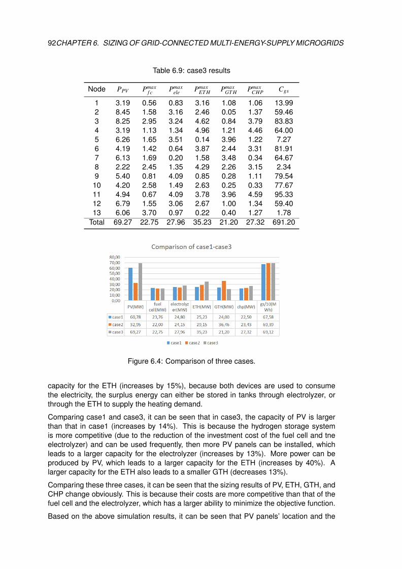
92CHAPTER 6. SIZING OF GRID-CONNECTED MULTI-ENERGY-SUPPLY MICROGRIDS
Table 6.9: case3 results
Node PPV Pmaxf c Pmax
ele PmaxET H Pmax
GT H PmaxCHP Cgs
1 3.19 0.56 0.83 3.16 1.08 1.06 13.992 8.45 1.58 3.16 2.46 0.05 1.37 59.463 8.25 2.95 3.24 4.62 0.84 3.79 83.834 3.19 1.13 1.34 4.96 1.21 4.46 64.005 6.26 1.65 3.51 0.14 3.96 1.22 7.276 4.19 1.42 0.64 3.87 2.44 3.31 81.917 6.13 1.69 0.20 1.58 3.48 0.34 64.678 2.22 2.45 1.35 4.29 2.26 3.15 2.349 5.40 0.81 4.09 0.85 0.28 1.11 79.54
10 4.20 2.58 1.49 2.63 0.25 0.33 77.6711 4.94 0.67 4.09 3.78 3.96 4.59 95.3312 6.79 1.55 3.06 2.67 1.00 1.34 59.4013 6.06 3.70 0.97 0.22 0.40 1.27 1.78
Total 69.27 22.75 27.96 35.23 21.20 27.32 691.20
Figure 6.4: Comparison of three cases.
capacity for the ETH (increases by 15%), because both devices are used to consumethe electricity, the surplus energy can either be stored in tanks through electrolyzer, orthrough the ETH to supply the heating demand.
Comparing case1 and case3, it can be seen that in case3, the capacity of PV is largerthan that in case1 (increases by 14%). This is because the hydrogen storage systemis more competitive (due to the reduction of the investment cost of the fuel cell and tneelectrolyzer) and can be used frequently, then more PV panels can be installed, whichleads to a larger capacity for the electrolyzer (increases by 13%). More power can beproduced by PV, which leads to a larger capacity for the ETH (increases by 40%). Alarger capacity for the ETH also leads to a smaller GTH (decreases 13%).
Comparing these three cases, it can be seen that the sizing results of PV, ETH, GTH, andCHP change obviously. This is because their costs are more competitive than that of thefuel cell and the electrolyzer, which has a larger ability to minimize the objective function.
Based on the above simulation results, it can be seen that PV panels’ location and the
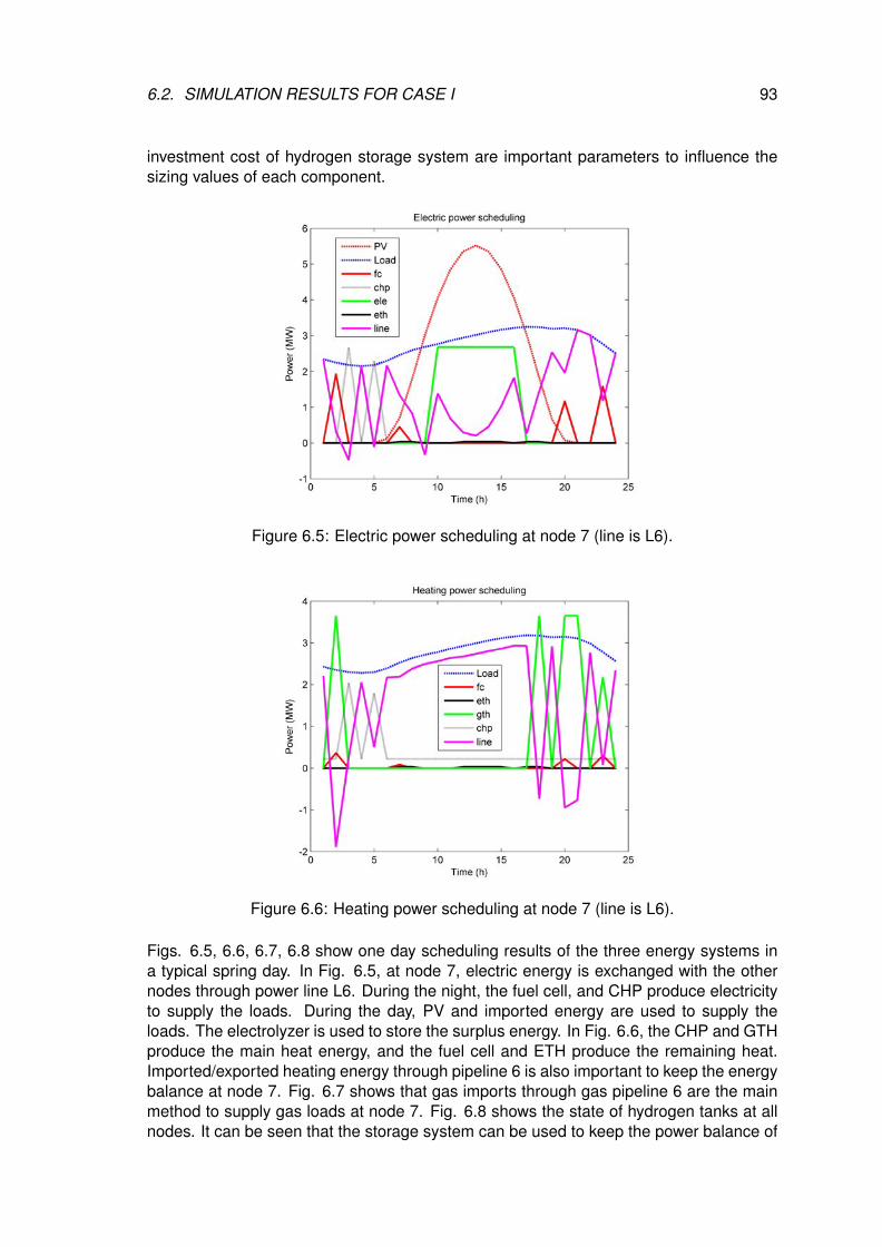
6.2. SIMULATION RESULTS FOR CASE I 93
investment cost of hydrogen storage system are important parameters to influence thesizing values of each component.
Figure 6.5: Electric power scheduling at node 7 (line is L6).
Figure 6.6: Heating power scheduling at node 7 (line is L6).
Figs. 6.5, 6.6, 6.7, 6.8 show one day scheduling results of the three energy systems ina typical spring day. In Fig. 6.5, at node 7, electric energy is exchanged with the othernodes through power line L6. During the night, the fuel cell, and CHP produce electricityto supply the loads. During the day, PV and imported energy are used to supply theloads. The electrolyzer is used to store the surplus energy. In Fig. 6.6, the CHP and GTHproduce the main heat energy, and the fuel cell and ETH produce the remaining heat.Imported/exported heating energy through pipeline 6 is also important to keep the energybalance at node 7. Fig. 6.7 shows that gas imports through gas pipeline 6 are the mainmethod to supply gas loads at node 7. Fig. 6.8 shows the state of hydrogen tanks at allnodes. It can be seen that the storage system can be used to keep the power balance of
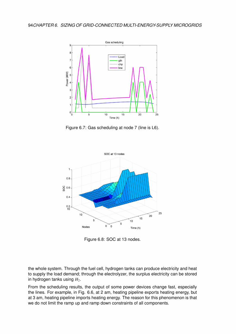
94CHAPTER 6. SIZING OF GRID-CONNECTED MULTI-ENERGY-SUPPLY MICROGRIDS
Figure 6.7: Gas scheduling at node 7 (line is L6).
Figure 6.8: SOC at 13 nodes.
the whole system. Through the fuel cell, hydrogen tanks can produce electricity and heatto supply the load demand; through the electrolyzer, the surplus electricity can be storedin hydrogen tanks using H2.
From the scheduling results, the output of some power devices change fast, especiallythe lines. For example, in Fig. 6.6, at 2 am, heating pipeline exports heating energy, butat 3 am, heating pipeline imports heating energy. The reason for this phenomenon is thatwe do not limit the ramp up and ramp down constraints of all components.
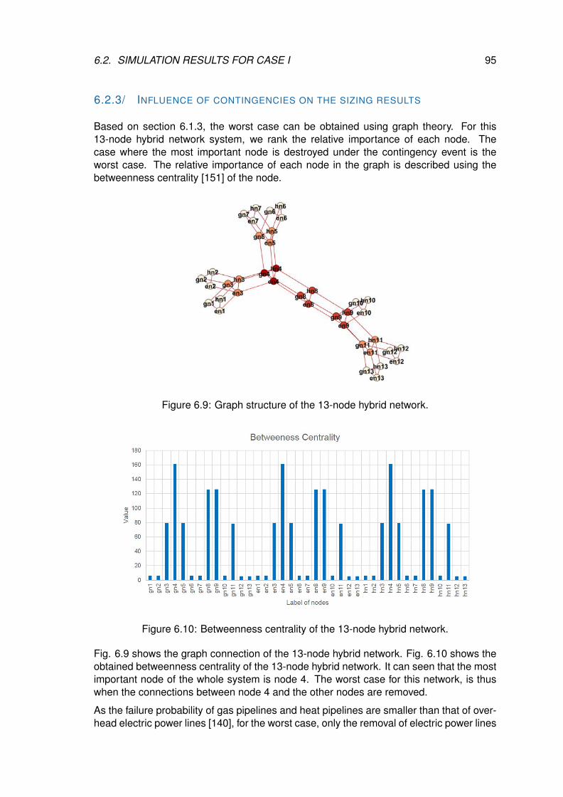
6.2. SIMULATION RESULTS FOR CASE I 95
6.2.3/ INFLUENCE OF CONTINGENCIES ON THE SIZING RESULTS
Based on section 6.1.3, the worst case can be obtained using graph theory. For this13-node hybrid network system, we rank the relative importance of each node. Thecase where the most important node is destroyed under the contingency event is theworst case. The relative importance of each node in the graph is described using thebetweenness centrality [151] of the node.
Figure 6.9: Graph structure of the 13-node hybrid network.
Figure 6.10: Betweenness centrality of the 13-node hybrid network.
Fig. 6.9 shows the graph connection of the 13-node hybrid network. Fig. 6.10 shows theobtained betweenness centrality of the 13-node hybrid network. It can seen that the mostimportant node of the whole system is node 4. The worst case for this network, is thuswhen the connections between node 4 and the other nodes are removed.
As the failure probability of gas pipelines and heat pipelines are smaller than that of over-head electric power lines [140], for the worst case, only the removal of electric power lines
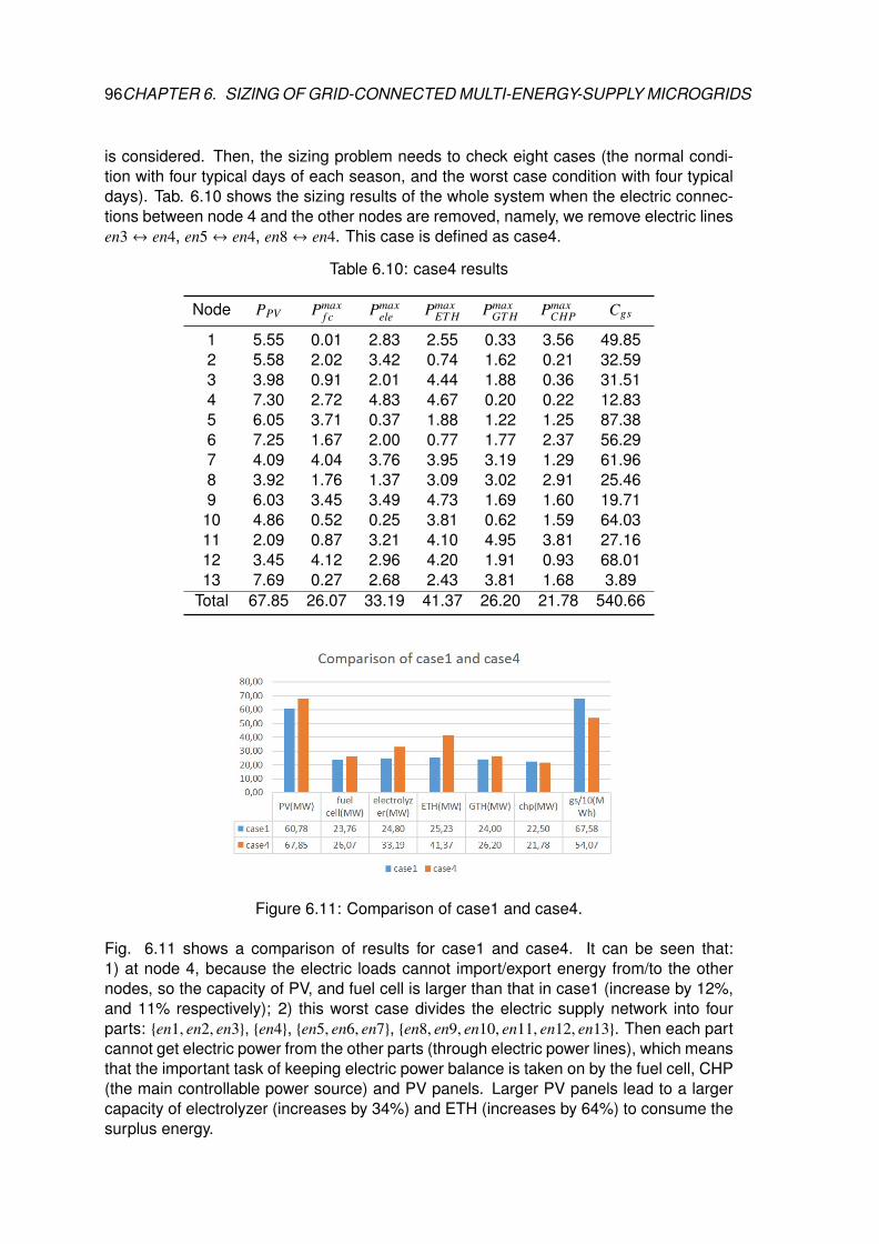
96CHAPTER 6. SIZING OF GRID-CONNECTED MULTI-ENERGY-SUPPLY MICROGRIDS
is considered. Then, the sizing problem needs to check eight cases (the normal condi-tion with four typical days of each season, and the worst case condition with four typicaldays). Tab. 6.10 shows the sizing results of the whole system when the electric connec-tions between node 4 and the other nodes are removed, namely, we remove electric linesen3↔ en4, en5↔ en4, en8↔ en4. This case is defined as case4.
Table 6.10: case4 results
Node PPV Pmaxf c Pmax
ele PmaxET H Pmax
GT H PmaxCHP Cgs
1 5.55 0.01 2.83 2.55 0.33 3.56 49.852 5.58 2.02 3.42 0.74 1.62 0.21 32.593 3.98 0.91 2.01 4.44 1.88 0.36 31.514 7.30 2.72 4.83 4.67 0.20 0.22 12.835 6.05 3.71 0.37 1.88 1.22 1.25 87.386 7.25 1.67 2.00 0.77 1.77 2.37 56.297 4.09 4.04 3.76 3.95 3.19 1.29 61.968 3.92 1.76 1.37 3.09 3.02 2.91 25.469 6.03 3.45 3.49 4.73 1.69 1.60 19.71
10 4.86 0.52 0.25 3.81 0.62 1.59 64.0311 2.09 0.87 3.21 4.10 4.95 3.81 27.1612 3.45 4.12 2.96 4.20 1.91 0.93 68.0113 7.69 0.27 2.68 2.43 3.81 1.68 3.89
Total 67.85 26.07 33.19 41.37 26.20 21.78 540.66
Figure 6.11: Comparison of case1 and case4.
Fig. 6.11 shows a comparison of results for case1 and case4. It can be seen that:1) at node 4, because the electric loads cannot import/export energy from/to the othernodes, so the capacity of PV, and fuel cell is larger than that in case1 (increase by 12%,and 11% respectively); 2) this worst case divides the electric supply network into fourparts: {en1, en2, en3}, {en4}, {en5, en6, en7}, {en8, en9, en10, en11, en12, en13}. Then each partcannot get electric power from the other parts (through electric power lines), which meansthat the important task of keeping electric power balance is taken on by the fuel cell, CHP(the main controllable power source) and PV panels. Larger PV panels lead to a largercapacity of electrolyzer (increases by 34%) and ETH (increases by 64%) to consume thesurplus energy.
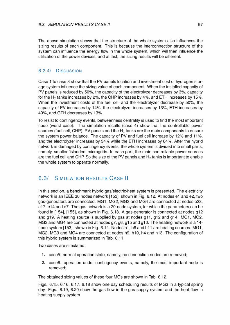
6.3. SIMULATION RESULTS CASE II 97
The above simulation shows that the structure of the whole system also influences thesizing results of each component. This is because the interconnection structure of thesystem can influence the energy flow in the whole system, which will then influence theutilization of the power devices, and at last, the sizing results will be different.
6.2.4/ DISCUSSION
Case 1 to case 3 show that the PV panels location and investment cost of hydrogen stor-age system influence the sizing value of each component. When the installed capacity ofPV panels is reduced by 50%, the capacity of the electrolyzer decreases by 3%, capacityfor the H2 tanks increases by 2%, the CHP increases by 4%, and ETH increases by 15%.When the investment costs of the fuel cell and the electrolyzer decrease by 50%, thecapacity of PV increases by 14%, the electrolyzer increases by 13%, ETH increases by40%, and GTH decreases by 13%.
To resist to contingency events, betweenness centrality is used to find the most importantnode (worst case). The simulation results (case 4) show that the controllable powersources (fuel cell, CHP), PV panels and the H2 tanks are the main components to ensurethe system power balance. The capacity of PV and fuel cell increase by 12% and 11%,and the electrolyzer increases by 34% while the ETH increases by 64%. After the hybridnetwork is damaged by contingency events, the whole system is divided into small parts,namely, smaller ’islanded’ microgrids. In each part, the main controllable power sourcesare the fuel cell and CHP. So the size of the PV panels and H2 tanks is important to enablethe whole system to operate normally.
6.3/ SIMULATION RESULTS CASE II
In this section, a benchmark hybrid gas/electric/heat system is presented. The electricitynetwork is an IEEE 30 nodes network [153], shown in Fig. 6.12. At nodes e1 and e2, twogas-generators are connected. MG1, MG2, MG3 and MG4 are connected at nodes e23,e17, e14 and e7. The gas network is a 20-node system, for which the parameters can befound in [154], [155], as shown in Fig. 6.13. A gas-generator is connected at nodes g12and g19. A heating source is supplied by gas at nodes g11, g12 and g14. MG1, MG2,MG3 and MG4 are connected at nodes g7, g6, g15 and g10. The heating network is a 14-node system [153], shown in Fig. 6.14. Nodes h1, h6 and h11 are heating sources. MG1,MG2, MG3 and MG4 are connected at nodes h9, h10, h4 and h13. The configuration ofthis hybrid system is summarized in Tab. 6.11.
Two cases are simulated:
1. case5: normal operation state, namely, no connection nodes are removed;
2. case6: operation under contingency events, namely, the most important node isremoved;
The obtained sizing values of these four MGs are shown in Tab. 6.12.
Figs. 6.15, 6.16, 6.17, 6.18 show one day scheduling results of MG3 in a typical springday. Figs. 6.19, 6.20 show the gas flow in the gas supply system and the heat flow inheating supply system.
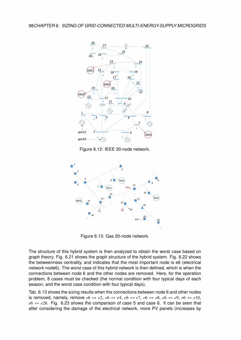
98CHAPTER 6. SIZING OF GRID-CONNECTED MULTI-ENERGY-SUPPLY MICROGRIDS
Figure 6.12: IEEE 30-node network.
Figure 6.13: Gas 20-node network.
The structure of this hybrid system is then analyzed to obtain the worst case based ongraph theory. Fig. 6.21 shows the graph structure of the hybrid system. Fig. 6.22 showsthe betweenness centrality, and indicates that the most important node is e6 (electricalnetwork node6). The worst case of this hybrid network is then defined, which is when theconnections between node 6 and the other nodes are removed. Here, for the operationproblem, 8 cases must be checked (the normal condition with four typical days of eachseason, and the worst case condition with four typical days).
Tab. 6.13 shows the sizing results when the connections between node 6 and other nodesis removed, namely, remove e6 ↔ e2, e6 ↔ e4, e6 ↔ e7, e6 ↔ e8, e6 ↔ e9, e6 ↔ e10,e6 ↔ e28. Fig. 6.23 shows the comparison of case 5 and case 6. It can be seen thatafter considering the damage of the electrical network, more PV panels (increases by
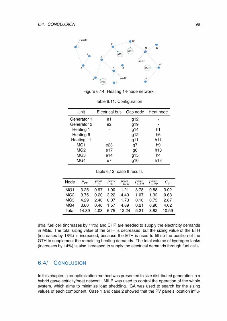
6.4. CONCLUSION 99
Figure 6.14: Heating 14-node network.
Table 6.11: Configuration
Unit Electrical bus Gas node Heat node
Generator 1 e1 g12 -Generator 2 e2 g19 -Heating 1 - g14 h1Heating 6 - g12 h6
Heating 11 - g11 h11MG1 e23 g7 h9MG2 e17 g6 h10MG3 e14 g15 h4MG4 e7 g10 h13
Table 6.12: case II results
Node PPV Pmaxf c Pmax
ele PmaxET H Pmax
GT H PmaxCHP Cgs
MG1 3.25 0.97 1.90 1.21 3.78 0.88 3.02MG2 3.75 0.20 3.22 4.40 1.07 1.32 0.68MG3 4.29 2.40 0.07 1.73 0.16 0.73 2.87MG4 3.60 0.46 1.57 4.89 0.21 0.90 4.02Total 14.89 4.03 6.75 12.24 5.21 3.82 10.59
8%), fuel cell (increases by 11%) and CHP are needed to supply the electricity demandsin MGs. The total sizing value of the GTH is decreased, but the sizing value of the ETH(increases by 18%) is increased, because the ETH is used to fill up the position of theGTH to supplement the remaining heating demands. The total volume of hydrogen tanks(increases by 14%) is also increased to supply the electrical demands through fuel cells.
6.4/ CONCLUSION
In this chapter, a co-optimization method was presented to size distributed generation in ahybrid gas/electricity/heat network. MILP was used to control the operation of the wholesystem, which aims to minimize load shedding. GA was used to search for the sizingvalues of each component. Case 1 and case 2 showed that the PV panels location influ-
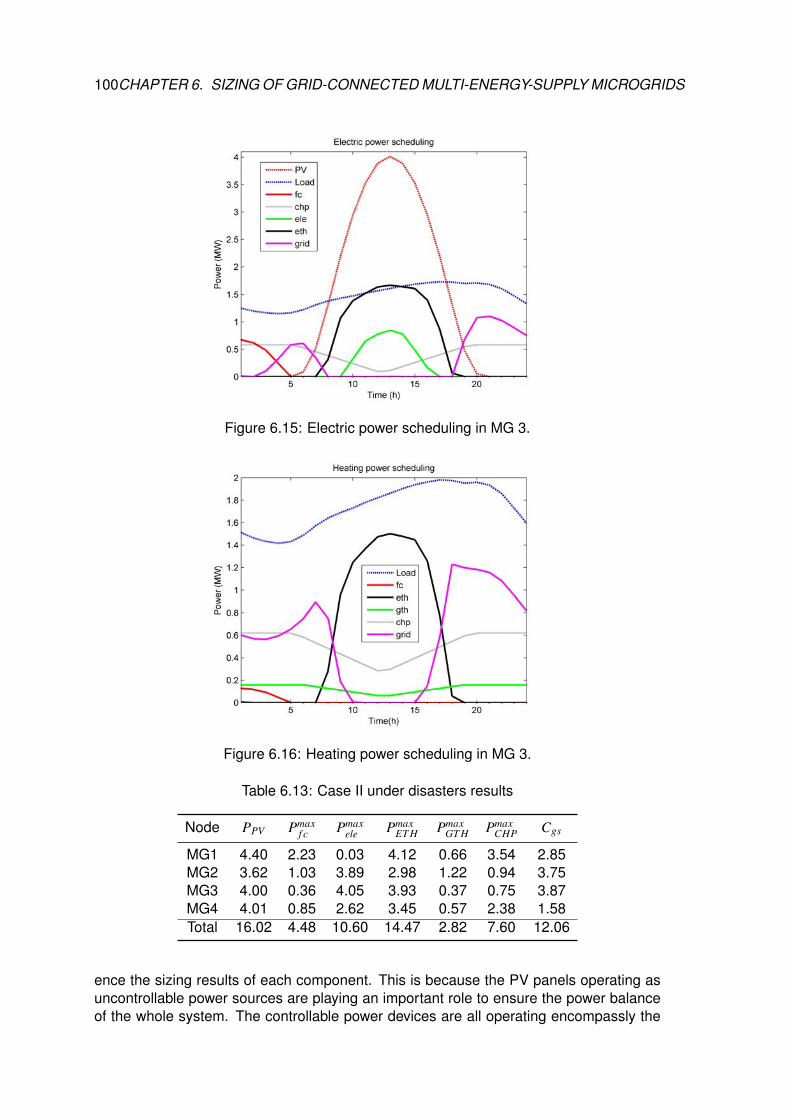
100CHAPTER 6. SIZING OF GRID-CONNECTED MULTI-ENERGY-SUPPLY MICROGRIDS
Figure 6.15: Electric power scheduling in MG 3.
Figure 6.16: Heating power scheduling in MG 3.
Table 6.13: Case II under disasters results
Node PPV Pmaxf c Pmax
ele PmaxET H Pmax
GT H PmaxCHP Cgs
MG1 4.40 2.23 0.03 4.12 0.66 3.54 2.85MG2 3.62 1.03 3.89 2.98 1.22 0.94 3.75MG3 4.00 0.36 4.05 3.93 0.37 0.75 3.87MG4 4.01 0.85 2.62 3.45 0.57 2.38 1.58Total 16.02 4.48 10.60 14.47 2.82 7.60 12.06
ence the sizing results of each component. This is because the PV panels operating asuncontrollable power sources are playing an important role to ensure the power balanceof the whole system. The controllable power devices are all operating encompassly the
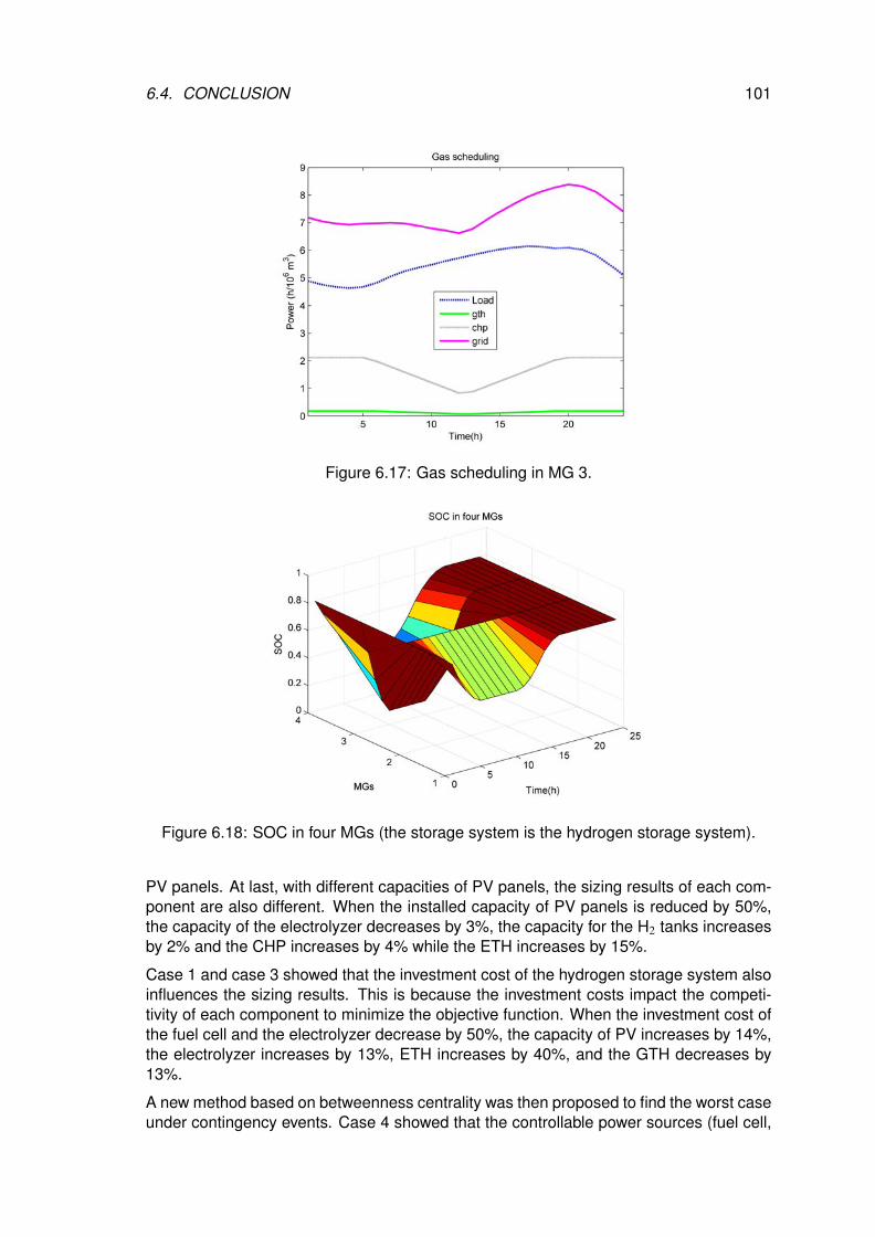
6.4. CONCLUSION 101
Figure 6.17: Gas scheduling in MG 3.
Figure 6.18: SOC in four MGs (the storage system is the hydrogen storage system).
PV panels. At last, with different capacities of PV panels, the sizing results of each com-ponent are also different. When the installed capacity of PV panels is reduced by 50%,the capacity of the electrolyzer decreases by 3%, the capacity for the H2 tanks increasesby 2% and the CHP increases by 4% while the ETH increases by 15%.
Case 1 and case 3 showed that the investment cost of the hydrogen storage system alsoinfluences the sizing results. This is because the investment costs impact the competi-tivity of each component to minimize the objective function. When the investment cost ofthe fuel cell and the electrolyzer decrease by 50%, the capacity of PV increases by 14%,the electrolyzer increases by 13%, ETH increases by 40%, and the GTH decreases by13%.
A new method based on betweenness centrality was then proposed to find the worst caseunder contingency events. Case 4 showed that the controllable power sources (fuel cell,
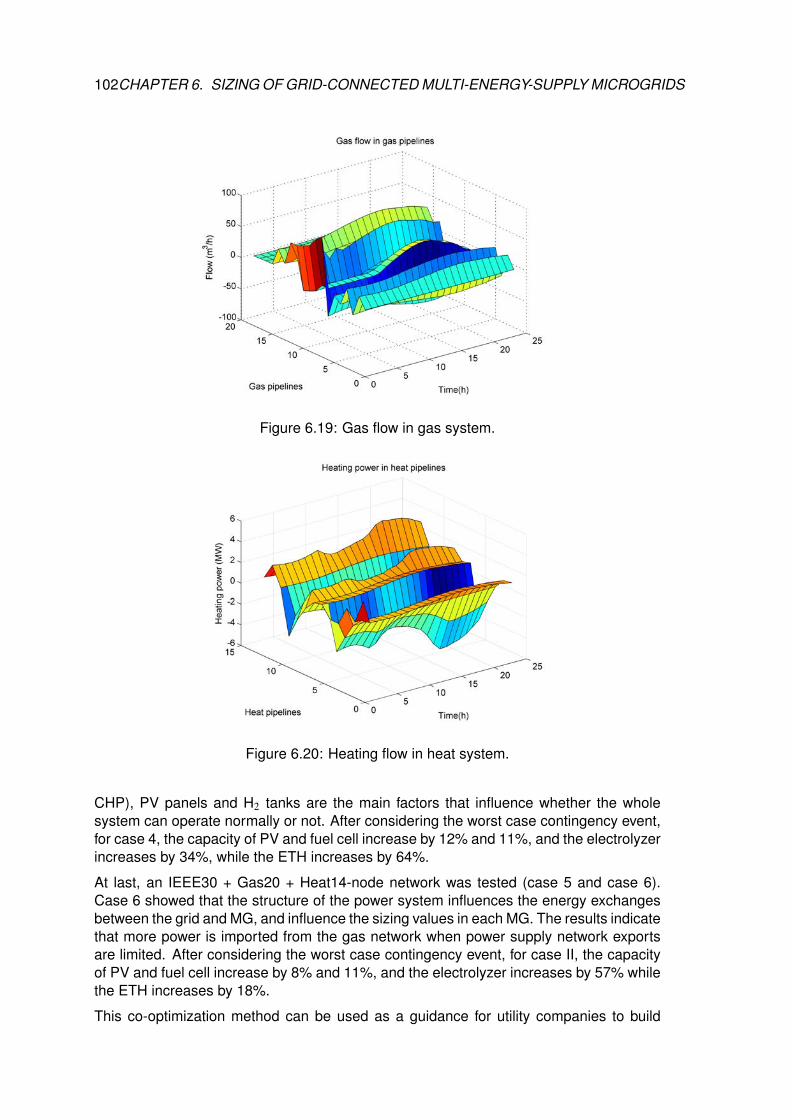
102CHAPTER 6. SIZING OF GRID-CONNECTED MULTI-ENERGY-SUPPLY MICROGRIDS
Figure 6.19: Gas flow in gas system.
Figure 6.20: Heating flow in heat system.
CHP), PV panels and H2 tanks are the main factors that influence whether the wholesystem can operate normally or not. After considering the worst case contingency event,for case 4, the capacity of PV and fuel cell increase by 12% and 11%, and the electrolyzerincreases by 34%, while the ETH increases by 64%.
At last, an IEEE30 + Gas20 + Heat14-node network was tested (case 5 and case 6).Case 6 showed that the structure of the power system influences the energy exchangesbetween the grid and MG, and influence the sizing values in each MG. The results indicatethat more power is imported from the gas network when power supply network exportsare limited. After considering the worst case contingency event, for case II, the capacityof PV and fuel cell increase by 8% and 11%, and the electrolyzer increases by 57% whilethe ETH increases by 18%.
This co-optimization method can be used as a guidance for utility companies to build
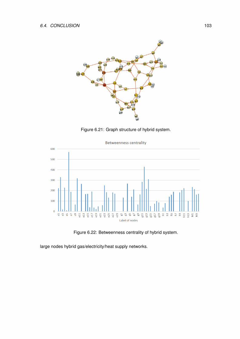
6.4. CONCLUSION 103
Figure 6.21: Graph structure of hybrid system.
Figure 6.22: Betweenness centrality of hybrid system.
large nodes hybrid gas/electricity/heat supply networks.
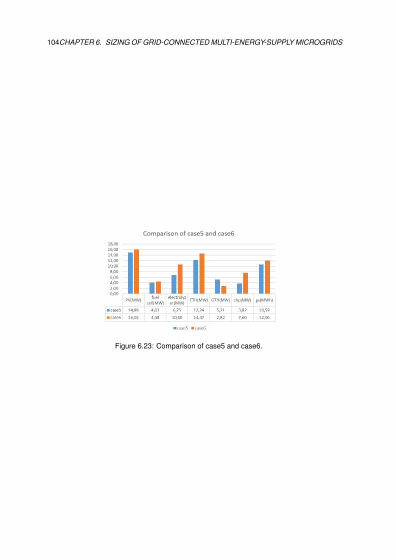
104CHAPTER 6. SIZING OF GRID-CONNECTED MULTI-ENERGY-SUPPLY MICROGRIDS
Figure 6.23: Comparison of case5 and case6.
7SIZING AND PRICE DECISION
ALGORITHM FOR GRID-CONNECTEDMICROGRIDS
The previous chapter discussed about the sizing problem of grid-connected microgrids.But we did not consider the electricity price. Actually, when microgrids interconnect
with the utility grid, microgrids will exchange energy with it based on the price. In thischapter, we research about the price decision approach for multiple grid-connected MESMGs. After that, we present a sizing algorithm for grid-connected MES MGs based onthe different prices.
Firstly, we introduce the load service entity (LSE) definition. Local generation, local stor-age systems and renewable energy sources can form an LSE, which can provide ancillaryservices to the utility grid (UG) and consumers. For example, when there is unbalancepower in the regulating power market, an LSE can provide upward/downward power tocompensate the imbalances. An LSE can also provide an incentive price to consumersto encourage them to participate in the market [131]. On the other hand, an MG can alsosell energy to the UG or LSE to earn profits. Then how the LSE can decide the electricityselling price to multiple MGs, and how the MGs can decide the selling price to LSE areproblems. The goal of deciding the prices for LSE and MGs is because prices are theonly way to guide the operation of LSE and UGs to arrange their energy scheduling. Theoperation of the LSE and MGs are significantly influenced by the prices. This meansthat different goals (such as shifting peak load, or improving the efficiency of the wholesystem) can be achieved by deploying different prices.
For an LSE, the goal is to maximize the profits, which includes local storage operationcosts, electricity buying costs from UG and MGs, and the profit earnings from MGs. Foreach MG, the goal is to minimize the costs, which includes the operation cost of eachcomponent, the electricity buying cost from the UG, and the profit earnings from an LSE.In this chapter, we present a price decision method for multiple MGs considering demandresponse. MILP is used to control the operation of each MG, and also used to operate theLSE. A GA is used to search for the best price for each MG and the LSE. This combinedmethod is deployed in a decentralized way, namely, each MG runs its own operationproblem. Compared to centralized control, the privacy of consumers can be protected.
The structure of the UG-LSE-MGs system is shown in Fig. 7.1. The LSE can purchaseelectricity from the utility grid, and with local generation and local storage systems, it canalso provide services to multiple MGs. In an LSE, renewable energy (PV) is integrated,
105
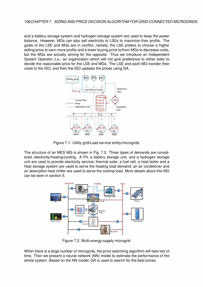
106CHAPTER 7. SIZING AND PRICE DECISION ALGORITHM FOR GRID-CONNECTED MICROGRIDS
and a battery storage system and hydrogen storage system are used to keep the powerbalance. However, MGs can also sell electricity to LSEs to maximize their profits. Thegoals of the LSE and MGs are in conflict, namely, the LSE prefers to choose a higherselling price to earn more profits and a lower buying price to/from MGs to decrease costs,but the MGs are actually aiming for the opposite. Thus we introduce an IndependentSystem Operator (i.e., an organization which will not give preference to either side) todecide the reasonable price for the LSE and MGs. The LSE and each MG transfer theircosts to the ISO, and then the ISO updates the prices using GA.
Figure 7.1: Utility grid/Load service entity/microgrids.
The structure of an MES MG is shown in Fig. 7.2. Three types of demands are consid-ered, electricity/heating/cooling. A PV, a battery storage unit, and a hydrogen storageunit are used to provide electricity service; thermal solar, a fuel cell, a heat boiler and aheat storage system are used to serve the heating load demand; an air conditioner andan absorption heat chiller are used to serve the cooling load. More details about this MGcan be seen in section 5.
Figure 7.2: Multi-energy-supply microgrid.
When there is a large number of microgrids, the price searching algorithm will take lots oftime. Then we present a neural network (NN) model to estimate the performance of thewhole system. Based on the NN model, GA is used to search for the best prices.
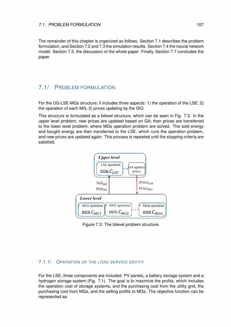
7.1. PROBLEM FORMULATION 107
The remainder of this chapter is organized as follows. Section 7.1 describes the problemformulation, and Section 7.2 and 7.3 the simulation results. Section 7.4 the neural networkmodel. Section 7.5, the discussion of the whole paper. Finally, Section 7.7 concludes thepaper.
7.1/ PROBLEM FORMULATION
For the UG-LSE-MGs structure, it includes three aspects: 1) the operation of the LSE; 2)the operation of each MG; 3) prices updating by the ISO.
This structure is formulated as a bilevel structure, which can be seen in Fig. 7.3. In theupper level problem, new prices are updated based on GA; then prices are transferredto the lower level problem, where MGs operation problem are solved. The sold energyand bought energy are then transferred to the LSE, which runs the operation problem,and new prices are updated again. This process is repeated until the stopping criteria aresatisfied.
Figure 7.3: The bilevel problem structure.
7.1.1/ OPERATION OF THE LOAD SERVICE ENTITY
For the LSE, three components are included: PV panels, a battery storage system and ahydrogen storage system (Fig. 7.1). The goal is to maximize the profits, which includesthe operation cost of storage systems, and the purchasing cost from the utility grid, thepurchasing cost from MGs, and the selling profits to MGs. The objective function can berepresented as:
108CHAPTER 7. SIZING AND PRICE DECISION ALGORITHM FOR GRID-CONNECTED MICROGRIDS
min CLS E =
minT∑
t=1
{Bch,discost (t) + Hele
cost(t) + H f ccost(t)
+ Priceug(t) · ug(t) +
N∑MGi=1
PriceMGi(t) · BuyMGi(t)
− PriceLS E(t) ·N∑
MGi=1
ZS ellMGi(t)
+ α · (LS ex(t)) + β · (cutPV (t))}
(7.1)
where the PriceLS E(t) is the selling price of LSE, PriceMGi(t) is the selling price of the ith
MG. ug(t) is the purchased energy from the utility grid, BuyMGi(t) is the bought energy fromthe ith MG. ZS ellMGi
(t) is the sold energy to the ith MG. LS ex(t) is the demands that cannotbe supplied by the LSE. cutPV (t) is the curtailed power of PV in the LSE.
For the battery storage system, the utilization cost of charge and discharge can be de-scribed as follows [142]:
Bch,discost (t) =
Cinvba
2 · Ncycles· (Pch(t) + Pdis(t)) (7.2)
where Cinvba is the investment cost of the battery, and Ncycles is the number of cycles over
the lifetime.
We use the state-of-charge (SOC) to represent the state of the battery as follows:
S OC(t) =S OC(t − ∆t)
+ηch · Pch(t) · ∆t
CB−ηdis · Pdis(t) · ∆t
CB
(7.3)
where ηch is the charging efficiency, ηdis is the discharging efficiency, Pch(t) is the chargingpower, Pdis(t) is the discharging power, ∆t is the interval time, and CB is the capacity ofthe battery.
The hydrogen storage system includes an electrolyzer, a fuel cell and hydrogen tanks. Asfor the battery storage system, its utilization cost can be computed as follows [142]:
Helecost(t) =
Cinvele
Nelehours
+ Co&mele
· δele(t) + Cstartupele · ∆δele(t) (7.4)
H f ccost(t) =
Cinvf c
N f chours
+ Co&mf c
· δ f c(t) + Cstartupf c · ∆δ f c(t) (7.5)
where Cinvele ,C
invf c are the investment costs of the electrolyzer and the fuel cell, Co&m
ele andCo&m
f c the operation and maintenance costs, and Cstartupele and Cstartup
f c the startup costs.Variables δele(t) and δ f c(t) are the state of the electrolyzer and the fuel cell. When a unit ison, δi(t) = 1, i = {ele, f c}, otherwise it is set to 0. Equation ∆δi(t) = max{δi(t)−δi(t−1), 0}, i =
{ele, f c} represents whether the unit started or not.
7.1. PROBLEM FORMULATION 109
A hydrogen tank is used to store the hydrogen produced by the electrolyzer, as well asto supply hydrogen to the fuel cell. We use the level of hydrogen (LOH) to represent thestate of the hydrogen tank:
LOH(t) = LOH(t − ∆t) + nproH2 · ∆t − ncon
H2 · ∆t (7.6)
where nproH2 is the hydrogen produced by electrolyzer. ncon
H2 is the hydrogen consumed byfuel cell. They can be calculated based on the method described in [142].
The electricity power balance equation is:
ug(t) +
N∑MGi=1
BuyMGi(t) + PV(t) − cutPV (t)
−
N∑MGi=1
ZS ellMGi(t) − LS ex(t)
= Zele(t) − Z f c(t) + Zbach(t) − Zbadis(t)
(7.7)
0 ≤ BuyMGi(t) ≤ ZBuyMGi(t) (7.8)
where ZBuyMGi(t) is the maximum selling energy of the ith MG at time t, which is obtained
from the results of problem (7.9). This means that at time t, an MG can sell ZBuyMGi(t)
amounts of energy, but for the LSE, how much it wants to buy is a variable, namelyBuyMGi(t).
At last, we need to decide the prices of PriceLS E(t) and PriceMGi(t), i = 1, ...,N.
7.1.2/ OPERATION OF MICROGRID
For each MG, the goal is to minimize the operation costs, which include the operationcosts of its own components, the purchasing cost from the LSE, and the selling profits tothe LSE. The objective function can be formulated as:
min CMGi =
minT∑
t=1
{Bch,discost (t) + Hele
cost(t) + H f ccost(t) + a1 · HBcost(t)+
a2 · ACcost(t) + AHCcost(t) + HS cost(t)
+ ω · (ZDRout (t) + ZDRin(t))
+ PriceLS E(t) · ZS ellMGi(t) − PriceMGi(t) · ZBuyMGi
(t)
+ α · (LS cooling(t) + LS heat(t) + LS power(t))
+ β · (cutPV (t) + cutsolar(t))}
(7.9)
where HBcost(t), ACcost(t), AHCcost(t),HS cost(t) are the utilization cost of the heat boiler, theair conditioner, the absorption heat chiller, and heat storage. ZDRout (t),ZDRin(t) are the shiftout power and shift in power, and ω is the DR cost. LS j(t), j = {cooling, heat, power} arethe load shedding of cooling, heating and electricity. cutPV (t), cutsolar(t) are the curtailed
110CHAPTER 7. SIZING AND PRICE DECISION ALGORITHM FOR GRID-CONNECTED MICROGRIDS
power of PV and thermal solar. α, β are the penalty values of load shedding and curtailedpower.
A heat boiler uses electricity to produce heat, as follows:
Qhb = ηhb · Phb (7.10)
where Phb is the input power, ηhb the efficiency, and Qhb the output heat.
An air conditioner is used to cool air [128]:
Cac = ηac · Pac (7.11)
where Pac is the input power, ηac the efficiency, and Cac the cooling output cooling power.
Similarly, the absorption heat chiller uses heat to produce cooling, so the relation is [128]:
Cahc = ηahc · Qahc (7.12)
where Qahc is the input heat, ηahc the efficiency, and Cahc the output cooling power.
The state of the heat storage system is represented by the amount of heat stored [63]:
HS (t) = HS (t − ∆t) + ηchhs · Q
chhs(t) · ∆t −
Qdishs (t)
ηdishs
· ∆t (7.13)
where HS (t) is the stored heat at time ∆t. Qchhs(t) and Qdis
hs (t) are the charge and dischargeheating power at time t. ηch
hs and ηdishs are the charge and discharge efficiency, respectively.
The heat boiler, air conditioner and absoption heat chiller operation costs are given by[141]:
HBcost(t) =Cinv
hb
Nhbli f e
· Phb(t) (7.14)
ACcost(t) =Cinv
ac
Nacli f e· Pac(t) (7.15)
AHCcost(t) =Cinv
ahc
Nahcli f e
· Pahc(t) (7.16)
For the heat storage system, the operation cost is:
HS cost(t) =Cinv
hs
Nhsli f e
· (Qchhs(t) + Qdis
hs (t)) (7.17)
The demand response model can be written as:
0 ≤ ZDRout (t) = δDRout (t) · PDRout (t) ≤ δDRout (t) · Pmaxload(t)
0 ≤ ZDRin(t) = δDRin(t) · PDRin(t) ≤ δDRin(t) · Pmaxin (t)
δDRout (t) + δDRin(t) ≤ 1
(7.18)
Shift-out power in each time step PDRout (t) is limited to Pmaxload(t); and shift-in power PDRin(t) is
limited to Pmaxin (t). δDRout (t) and δDRin(t) are binary variables that represent whether shift-out
power/shift-in power in this step is allowed or not.
7.1. PROBLEM FORMULATION 111
The electricity selling and buying in MG can be written as:
0 ≤ ZS ellMGi(t) ≤ δS ellMGi
(t) · S ellmax(t)
0 ≤ ZBuyMGi(t) ≤ δBuyMGi
(t) · Buymax(t)
δS ellMGi(t) + δBuyMGi
(t) ≤ 1
(7.19)
where ZS ellMGi(t) = δS ellMGi
(t) ·S ellMGi(t), ZBuyMGi(t) = δBuyMGi
(t) ·BuyMGi(t). δS ellMGi(t), δBuyMGi
(t)are binary variables that represent the state of buying energy and selling energy.
The electricity power balance in an MG can be described as:
ZS ellMGi(t) − ZBuyMGi
(t) + PV(t) − cutPV (t)
− (Lpower(t) − ZDRout (t) + ZDRin(t))
= Zele(t) − Z f c(t) + Zbach(t) − Zbadis(t)
+ Zac(t) + Zhb(t)
(7.20)
The shift-out power should be equal to the shift-in power:
T∑t=1
ZDRout (t) =
T∑t=1
ZDRin(t) (7.21)
Similarly, for the heat and cooling balance equations:
Qsh(t) − cutsolar(t) − (Lheat(t) − LS heat(t)) + Q f c(t)
+ Qhb(t) = Qhsch(t) − Qhsdis(t) + Qahc(t)(7.22)
Cac(t) + Cahc(t) = Lcooling(t) − LS cooling(t) (7.23)
Finally, for the SOC, LOH and HS constraints:
S OCmin ≤ S OC(t) ≤ S OCmax
LOHmin ≤ LOH(t) ≤ LOHmax
HS min ≤ HS (t) ≤ HS max
(7.24)
7.1.3/ CONFLICTING GOALS OF LOAD SERVICE ENTITY AND MICROGRIDS
Based on the above, the objective functions of LSE and MGs are all to minimize the op-eration cost. But from problem (7.1) and problem (7.9), we can see that the decision vari-ables PriceLS E(t) and PriceMGi(t), i = 1, ...,N are conflicting variables from the LSE’s viewand MGs’ view. This means that the LSE prefers a higher LSE selling price PriceLS E(t)and a lower MGs selling price PriceMGi(t), i = 1, ...,N. But MGs prefer a lower LSE sellingprice PriceLS E(t) and a higher MGs selling price PriceMGi(t), i = 1, ...,N.
Here, a simulation example is adopted to describe the relationship between price(PriceLS E(t), PriceMGi(t), i = 1, ...,N) and operation cost. The results can be seen in Fig.
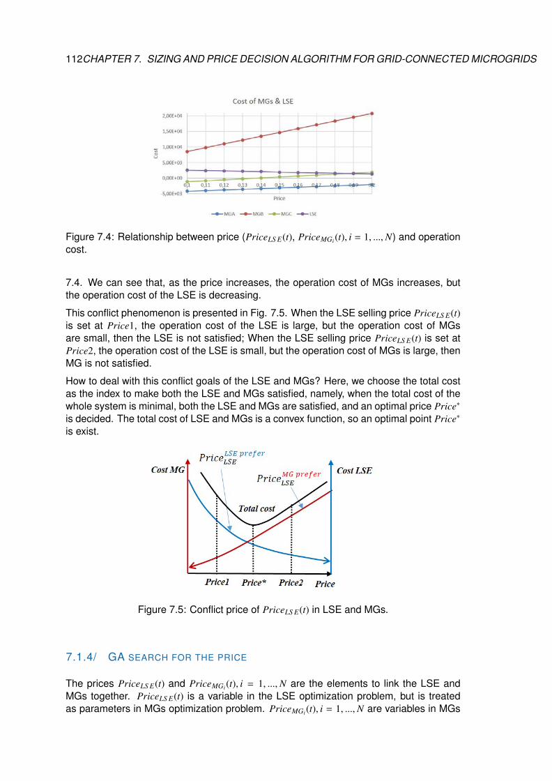
112CHAPTER 7. SIZING AND PRICE DECISION ALGORITHM FOR GRID-CONNECTED MICROGRIDS
Figure 7.4: Relationship between price (PriceLS E(t), PriceMGi(t), i = 1, ...,N) and operationcost.
7.4. We can see that, as the price increases, the operation cost of MGs increases, butthe operation cost of the LSE is decreasing.
This conflict phenomenon is presented in Fig. 7.5. When the LSE selling price PriceLS E(t)is set at Price1, the operation cost of the LSE is large, but the operation cost of MGsare small, then the LSE is not satisfied; When the LSE selling price PriceLS E(t) is set atPrice2, the operation cost of the LSE is small, but the operation cost of MGs is large, thenMG is not satisfied.
How to deal with this conflict goals of the LSE and MGs? Here, we choose the total costas the index to make both the LSE and MGs satisfied, namely, when the total cost of thewhole system is minimal, both the LSE and MGs are satisfied, and an optimal price Price∗
is decided. The total cost of LSE and MGs is a convex function, so an optimal point Price∗
is exist.
Figure 7.5: Conflict price of PriceLS E(t) in LSE and MGs.
7.1.4/ GA SEARCH FOR THE PRICE
The prices PriceLS E(t) and PriceMGi(t), i = 1, ...,N are the elements to link the LSE andMGs together. PriceLS E(t) is a variable in the LSE optimization problem, but is treatedas parameters in MGs optimization problem. PriceMGi(t), i = 1, ...,N are variables in MGs
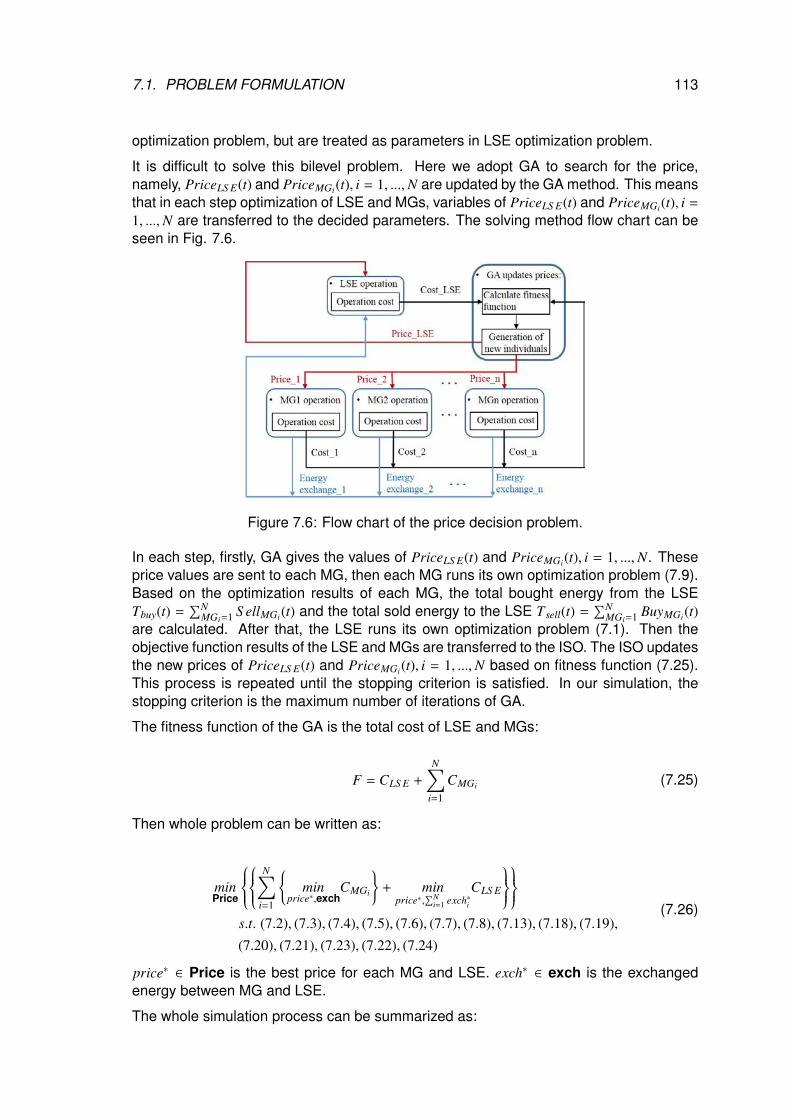
7.1. PROBLEM FORMULATION 113
optimization problem, but are treated as parameters in LSE optimization problem.
It is difficult to solve this bilevel problem. Here we adopt GA to search for the price,namely, PriceLS E(t) and PriceMGi(t), i = 1, ...,N are updated by the GA method. This meansthat in each step optimization of LSE and MGs, variables of PriceLS E(t) and PriceMGi(t), i =
1, ...,N are transferred to the decided parameters. The solving method flow chart can beseen in Fig. 7.6.
Figure 7.6: Flow chart of the price decision problem.
In each step, firstly, GA gives the values of PriceLS E(t) and PriceMGi(t), i = 1, ...,N. Theseprice values are sent to each MG, then each MG runs its own optimization problem (7.9).Based on the optimization results of each MG, the total bought energy from the LSETbuy(t) =
∑NMGi=1 S ellMGi(t) and the total sold energy to the LSE Tsell(t) =
∑NMGi=1 BuyMGi(t)
are calculated. After that, the LSE runs its own optimization problem (7.1). Then theobjective function results of the LSE and MGs are transferred to the ISO. The ISO updatesthe new prices of PriceLS E(t) and PriceMGi(t), i = 1, ...,N based on fitness function (7.25).This process is repeated until the stopping criterion is satisfied. In our simulation, thestopping criterion is the maximum number of iterations of GA.
The fitness function of the GA is the total cost of LSE and MGs:
F = CLS E +
N∑i=1
CMGi (7.25)
Then whole problem can be written as:
minPrice
N∑
i=1
{min
price∗,exchCMGi
}+ min
price∗,∑N
i=1 exch∗iCLS E
s.t. (7.2), (7.3), (7.4), (7.5), (7.6), (7.7), (7.8), (7.13), (7.18), (7.19),
(7.20), (7.21), (7.23), (7.22), (7.24)
(7.26)
price∗ ∈ Price is the best price for each MG and LSE. exch∗ ∈ exch is the exchangedenergy between MG and LSE.
The whole simulation process can be summarized as:
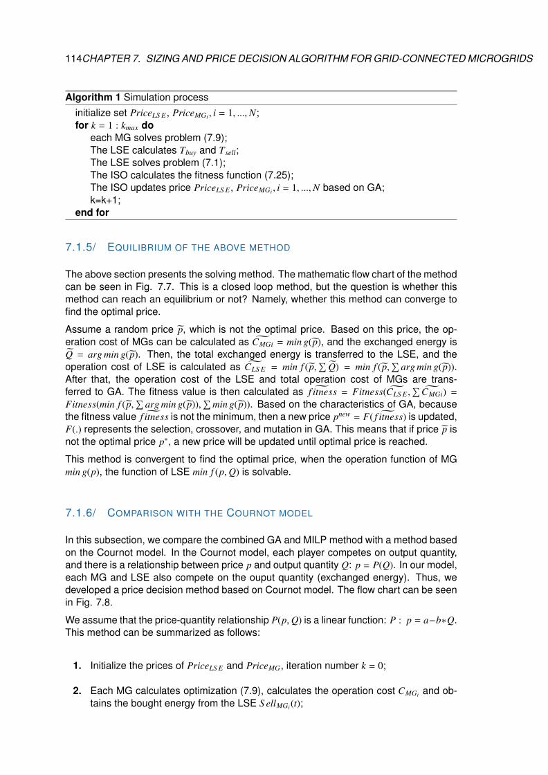
114CHAPTER 7. SIZING AND PRICE DECISION ALGORITHM FOR GRID-CONNECTED MICROGRIDS
Algorithm 1 Simulation processinitialize set PriceLS E, PriceMGi , i = 1, ...,N;for k = 1 : kmax do
each MG solves problem (7.9);The LSE calculates Tbuy and Tsell;The LSE solves problem (7.1);The ISO calculates the fitness function (7.25);The ISO updates price PriceLS E, PriceMGi , i = 1, ...,N based on GA;k=k+1;
end for
7.1.5/ EQUILIBRIUM OF THE ABOVE METHOD
The above section presents the solving method. The mathematic flow chart of the methodcan be seen in Fig. 7.7. This is a closed loop method, but the question is whether thismethod can reach an equilibrium or not? Namely, whether this method can converge tofind the optimal price.
Assume a random price p, which is not the optimal price. Based on this price, the op-eration cost of MGs can be calculated as CMGi = min g(p), and the exchanged energy isQ = arg min g( p). Then, the total exchanged energy is transferred to the LSE, and theoperation cost of LSE is calculated as CLS E = min f ( p,
∑Q) = min f ( p,
∑arg min g( p)).
After that, the operation cost of the LSE and total operation cost of MGs are trans-ferred to GA. The fitness value is then calculated as ˜f itness = Fitness(CLS E ,
∑CMGi) =
Fitness(min f ( p,∑
arg min g( p)),∑
min g(p)). Based on the characteristics of GA, becausethe fitness value ˜f itness is not the minimum, then a new price pnew = F( ˜f itness) is updated,F(.) represents the selection, crossover, and mutation in GA. This means that if price p isnot the optimal price p∗, a new price will be updated until optimal price is reached.
This method is convergent to find the optimal price, when the operation function of MGmin g(p), the function of LSE min f (p,Q) is solvable.
7.1.6/ COMPARISON WITH THE COURNOT MODEL
In this subsection, we compare the combined GA and MILP method with a method basedon the Cournot model. In the Cournot model, each player competes on output quantity,and there is a relationship between price p and output quantity Q: p = P(Q). In our model,each MG and LSE also compete on the ouput quantity (exchanged energy). Thus, wedeveloped a price decision method based on Cournot model. The flow chart can be seenin Fig. 7.8.
We assume that the price-quantity relationship P(p,Q) is a linear function: P : p = a−b∗Q.This method can be summarized as follows:
1. Initialize the prices of PriceLS E and PriceMG, iteration number k = 0;
2. Each MG calculates optimization (7.9), calculates the operation cost CMGi and ob-tains the bought energy from the LSE S ellMGi(t);
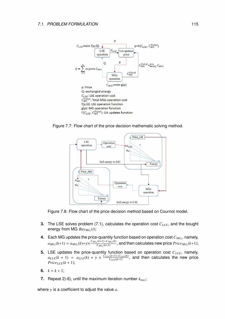
7.1. PROBLEM FORMULATION 115
Figure 7.7: Flow chart of the price decision mathematic solving method.
Figure 7.8: Flow chart of the price decision method based on Cournot model.
3. The LSE solves problem (7.1), calculates the operation cost CLS E, and the boughtenergy from MG BuyMGi(t);
4. Each MG updates the price-quantity function based on operation cost CMGi , namely,aMGi(k+1) = aMGi(k)+γ×
CMGi (k+1)−CMGi (k)CMGi (k+1) , and then calculates new price PriceMGi(k+1);
5. LSE updates the price-quantity function based on operation cost CLS E, namely,aLS E(k + 1) = aLS E(k) + γ × CLS E(k+1)−CLS E(k)
CLS E(k+1) , and then calculates the new pricePriceLS E(k + 1);
6. k = k + 1;
7. Repeat 2)-6), until the maximum iteration number kmax;
where γ is a coefficient to adjust the value a.
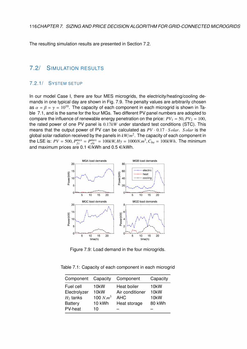
116CHAPTER 7. SIZING AND PRICE DECISION ALGORITHM FOR GRID-CONNECTED MICROGRIDS
The resulting simulation results are presented in Section 7.2.
7.2/ SIMULATION RESULTS
7.2.1/ SYSTEM SETUP
In our model Case I, there are four MES microgrids, the electricity/heating/cooling de-mands in one typical day are shown in Fig. 7.9. The penalty values are arbitrarily chosenas α = β = γ = 1010. The capacity of each component in each microgrid is shown in Ta-ble 7.1, and is the same for the four MGs. Two different PV panel numbers are adopted tocompare the influence of renewable energy penetration on the price: PV1 = 50, PV2 = 100,the rated power of one PV panel is 0.17kW under standard test conditions (STC). Thismeans that the output power of PV can be calculated as PV · 0.17 · S olar. S olar is theglobal solar radiation received by the panels in kW/m2. The capacity of each component inthe LSE is: PV = 500, Pmax
f c = Pmaxele = 100kW,Hy = 1000N.m3,Cba = 100kWh. The minimum
and maximum prices are 0.1 e/kWh and 0.5 e/kWh.
Figure 7.9: Load demand in the four microgrids.
Table 7.1: Capacity of each component in each microgrid
Component Capacity Component Capacity
Fuel cell 10kW Heat boiler 10kWElectrolyzer 10kW Air conditioner 10kWH2 tanks 100 N.m3 AHC 10kWBattery 10 kWh Heat storage 80 kWhPV-heat 10 – –
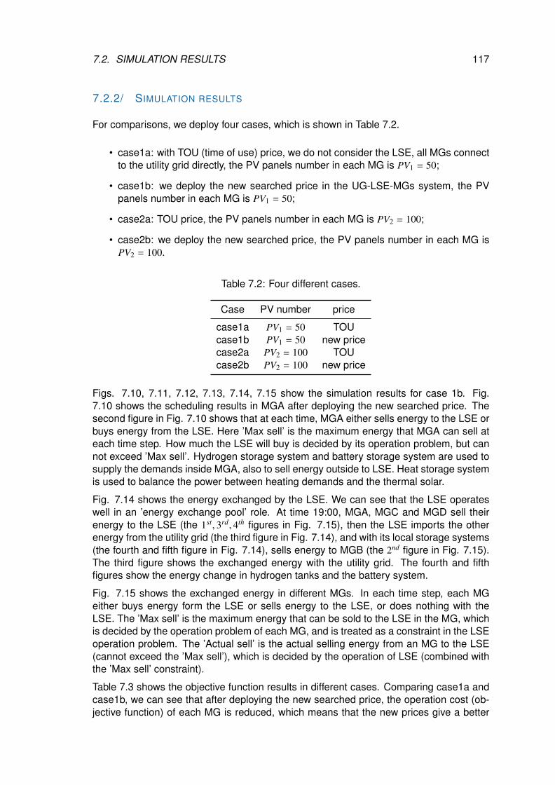
7.2. SIMULATION RESULTS 117
7.2.2/ SIMULATION RESULTS
For comparisons, we deploy four cases, which is shown in Table 7.2.
• case1a: with TOU (time of use) price, we do not consider the LSE, all MGs connectto the utility grid directly, the PV panels number in each MG is PV1 = 50;
• case1b: we deploy the new searched price in the UG-LSE-MGs system, the PVpanels number in each MG is PV1 = 50;
• case2a: TOU price, the PV panels number in each MG is PV2 = 100;
• case2b: we deploy the new searched price, the PV panels number in each MG isPV2 = 100.
Table 7.2: Four different cases.
Case PV number price
case1a PV1 = 50 TOUcase1b PV1 = 50 new pricecase2a PV2 = 100 TOUcase2b PV2 = 100 new price
Figs. 7.10, 7.11, 7.12, 7.13, 7.14, 7.15 show the simulation results for case 1b. Fig.7.10 shows the scheduling results in MGA after deploying the new searched price. Thesecond figure in Fig. 7.10 shows that at each time, MGA either sells energy to the LSE orbuys energy from the LSE. Here ’Max sell’ is the maximum energy that MGA can sell ateach time step. How much the LSE will buy is decided by its operation problem, but cannot exceed ’Max sell’. Hydrogen storage system and battery storage system are used tosupply the demands inside MGA, also to sell energy outside to LSE. Heat storage systemis used to balance the power between heating demands and the thermal solar.
Fig. 7.14 shows the energy exchanged by the LSE. We can see that the LSE operateswell in an ’energy exchange pool’ role. At time 19:00, MGA, MGC and MGD sell theirenergy to the LSE (the 1st, 3rd, 4th figures in Fig. 7.15), then the LSE imports the otherenergy from the utility grid (the third figure in Fig. 7.14), and with its local storage systems(the fourth and fifth figure in Fig. 7.14), sells energy to MGB (the 2nd figure in Fig. 7.15).The third figure shows the exchanged energy with the utility grid. The fourth and fifthfigures show the energy change in hydrogen tanks and the battery system.
Fig. 7.15 shows the exchanged energy in different MGs. In each time step, each MGeither buys energy form the LSE or sells energy to the LSE, or does nothing with theLSE. The ’Max sell’ is the maximum energy that can be sold to the LSE in the MG, whichis decided by the operation problem of each MG, and is treated as a constraint in the LSEoperation problem. The ’Actual sell’ is the actual selling energy from an MG to the LSE(cannot exceed the ’Max sell’), which is decided by the operation of LSE (combined withthe ’Max sell’ constraint).
Table 7.3 shows the objective function results in different cases. Comparing case1a andcase1b, we can see that after deploying the new searched price, the operation cost (ob-jective function) of each MG is reduced, which means that the new prices give a better
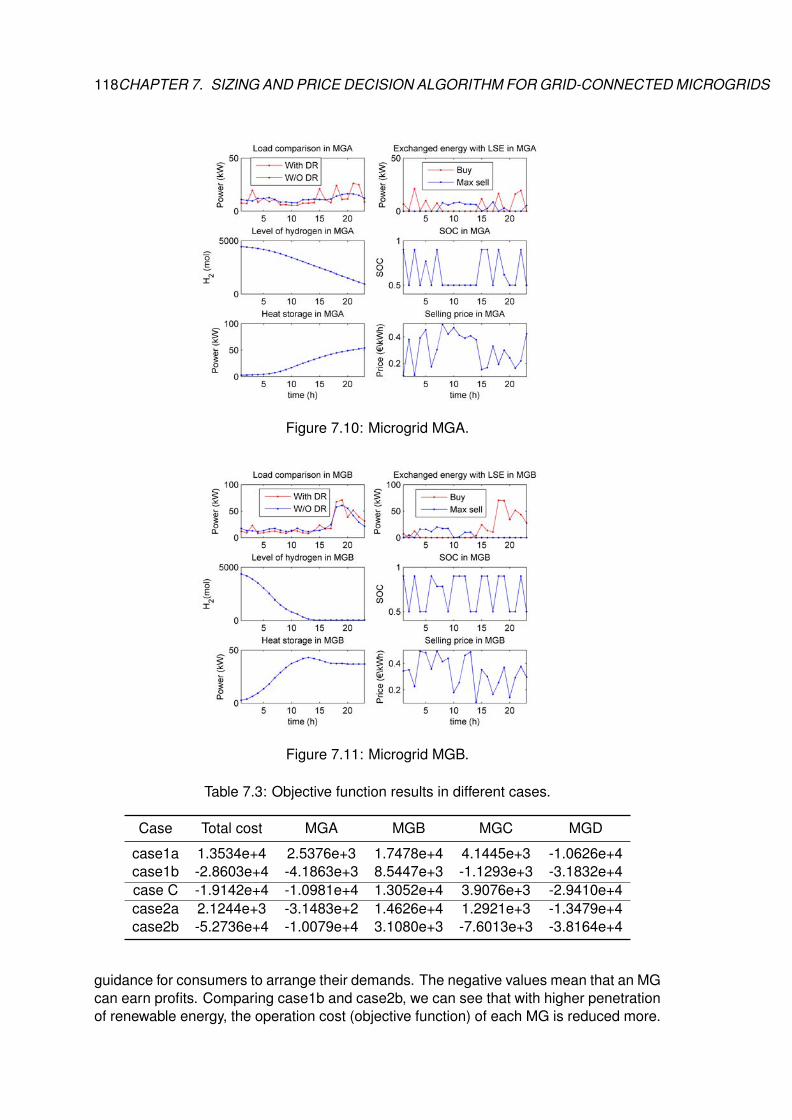
118CHAPTER 7. SIZING AND PRICE DECISION ALGORITHM FOR GRID-CONNECTED MICROGRIDS
Figure 7.10: Microgrid MGA.
Figure 7.11: Microgrid MGB.
Table 7.3: Objective function results in different cases.
Case Total cost MGA MGB MGC MGD
case1a 1.3534e+4 2.5376e+3 1.7478e+4 4.1445e+3 -1.0626e+4case1b -2.8603e+4 -4.1863e+3 8.5447e+3 -1.1293e+3 -3.1832e+4case C -1.9142e+4 -1.0981e+4 1.3052e+4 3.9076e+3 -2.9410e+4case2a 2.1244e+3 -3.1483e+2 1.4626e+4 1.2921e+3 -1.3479e+4case2b -5.2736e+4 -1.0079e+4 3.1080e+3 -7.6013e+3 -3.8164e+4
guidance for consumers to arrange their demands. The negative values mean that an MGcan earn profits. Comparing case1b and case2b, we can see that with higher penetrationof renewable energy, the operation cost (objective function) of each MG is reduced more.
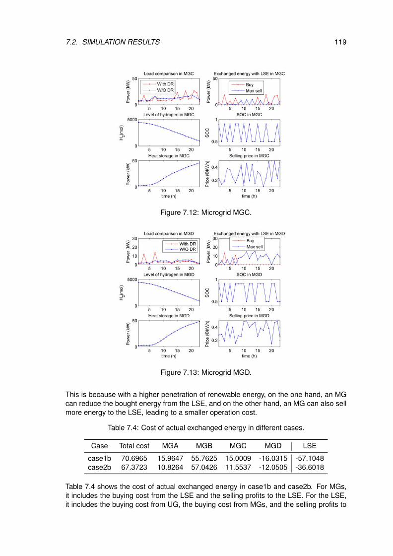
7.2. SIMULATION RESULTS 119
Figure 7.12: Microgrid MGC.
Figure 7.13: Microgrid MGD.
This is because with a higher penetration of renewable energy, on the one hand, an MGcan reduce the bought energy from the LSE, and on the other hand, an MG can also sellmore energy to the LSE, leading to a smaller operation cost.
Table 7.4: Cost of actual exchanged energy in different cases.
Case Total cost MGA MGB MGC MGD LSE
case1b 70.6965 15.9647 55.7625 15.0009 -16.0315 -57.1048case2b 67.3723 10.8264 57.0426 11.5537 -12.0505 -36.6018
Table 7.4 shows the cost of actual exchanged energy in case1b and case2b. For MGs,it includes the buying cost from the LSE and the selling profits to the LSE. For the LSE,it includes the buying cost from UG, the buying cost from MGs, and the selling profits to
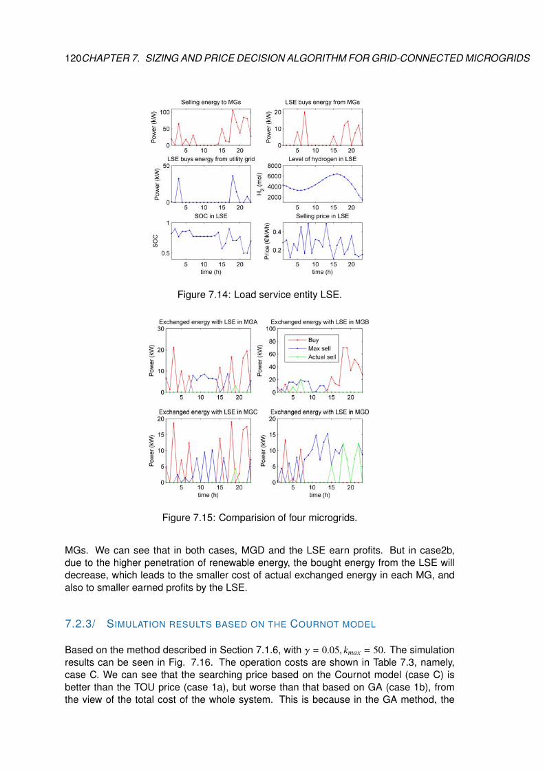
120CHAPTER 7. SIZING AND PRICE DECISION ALGORITHM FOR GRID-CONNECTED MICROGRIDS
Figure 7.14: Load service entity LSE.
Figure 7.15: Comparision of four microgrids.
MGs. We can see that in both cases, MGD and the LSE earn profits. But in case2b,due to the higher penetration of renewable energy, the bought energy from the LSE willdecrease, which leads to the smaller cost of actual exchanged energy in each MG, andalso to smaller earned profits by the LSE.
7.2.3/ SIMULATION RESULTS BASED ON THE COURNOT MODEL
Based on the method described in Section 7.1.6, with γ = 0.05, kmax = 50. The simulationresults can be seen in Fig. 7.16. The operation costs are shown in Table 7.3, namely,case C. We can see that the searching price based on the Cournot model (case C) isbetter than the TOU price (case 1a), but worse than that based on GA (case 1b), fromthe view of the total cost of the whole system. This is because in the GA method, the
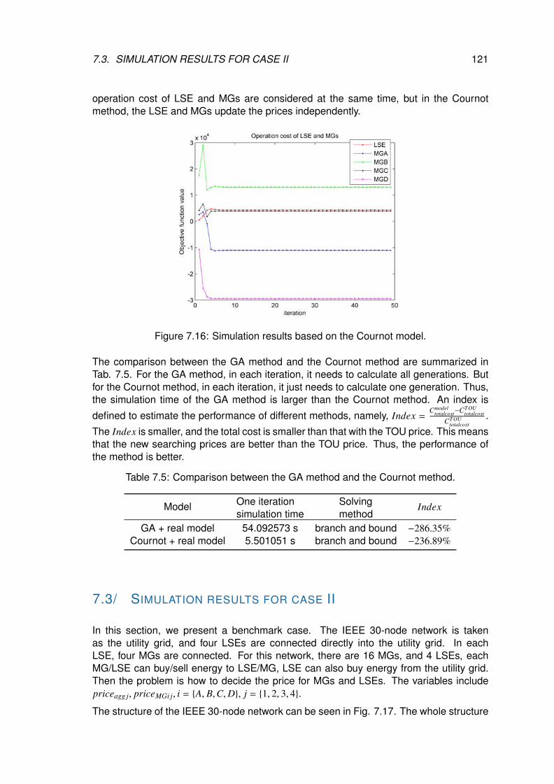
7.3. SIMULATION RESULTS FOR CASE II 121
operation cost of LSE and MGs are considered at the same time, but in the Cournotmethod, the LSE and MGs update the prices independently.
Figure 7.16: Simulation results based on the Cournot model.
The comparison between the GA method and the Cournot method are summarized inTab. 7.5. For the GA method, in each iteration, it needs to calculate all generations. Butfor the Cournot method, in each iteration, it just needs to calculate one generation. Thus,the simulation time of the GA method is larger than the Cournot method. An index is
defined to estimate the performance of different methods, namely, Index =Cmodel
totalcost−CTOUtotalcost
CTOUtotalcost
.
The Index is smaller, and the total cost is smaller than that with the TOU price. This meansthat the new searching prices are better than the TOU price. Thus, the performance ofthe method is better.
Table 7.5: Comparison between the GA method and the Cournot method.
Model One iterationsimulation time
Solvingmethod
Index
GA + real model 54.092573 s branch and bound −286.35%Cournot + real model 5.501051 s branch and bound −236.89%
7.3/ SIMULATION RESULTS FOR CASE II
In this section, we present a benchmark case. The IEEE 30-node network is takenas the utility grid, and four LSEs are connected directly into the utility grid. In eachLSE, four MGs are connected. For this network, there are 16 MGs, and 4 LSEs, eachMG/LSE can buy/sell energy to LSE/MG, LSE can also buy energy from the utility grid.Then the problem is how to decide the price for MGs and LSEs. The variables includepriceagg j, priceMGi j, i = {A, B,C,D}, j = {1, 2, 3, 4}.
The structure of the IEEE 30-node network can be seen in Fig. 7.17. The whole structure
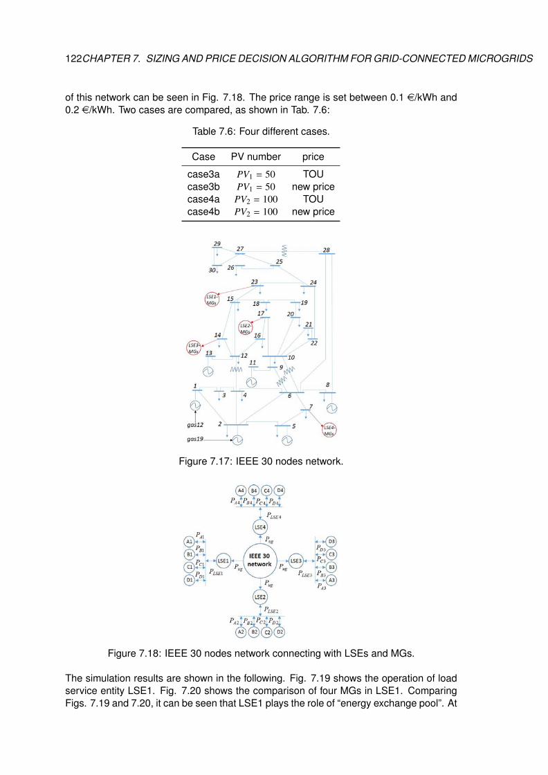
122CHAPTER 7. SIZING AND PRICE DECISION ALGORITHM FOR GRID-CONNECTED MICROGRIDS
of this network can be seen in Fig. 7.18. The price range is set between 0.1 e/kWh and0.2 e/kWh. Two cases are compared, as shown in Tab. 7.6:
Table 7.6: Four different cases.
Case PV number price
case3a PV1 = 50 TOUcase3b PV1 = 50 new pricecase4a PV2 = 100 TOUcase4b PV2 = 100 new price
Figure 7.17: IEEE 30 nodes network.
Figure 7.18: IEEE 30 nodes network connecting with LSEs and MGs.
The simulation results are shown in the following. Fig. 7.19 shows the operation of loadservice entity LSE1. Fig. 7.20 shows the comparison of four MGs in LSE1. ComparingFigs. 7.19 and 7.20, it can be seen that LSE1 plays the role of “energy exchange pool”. At
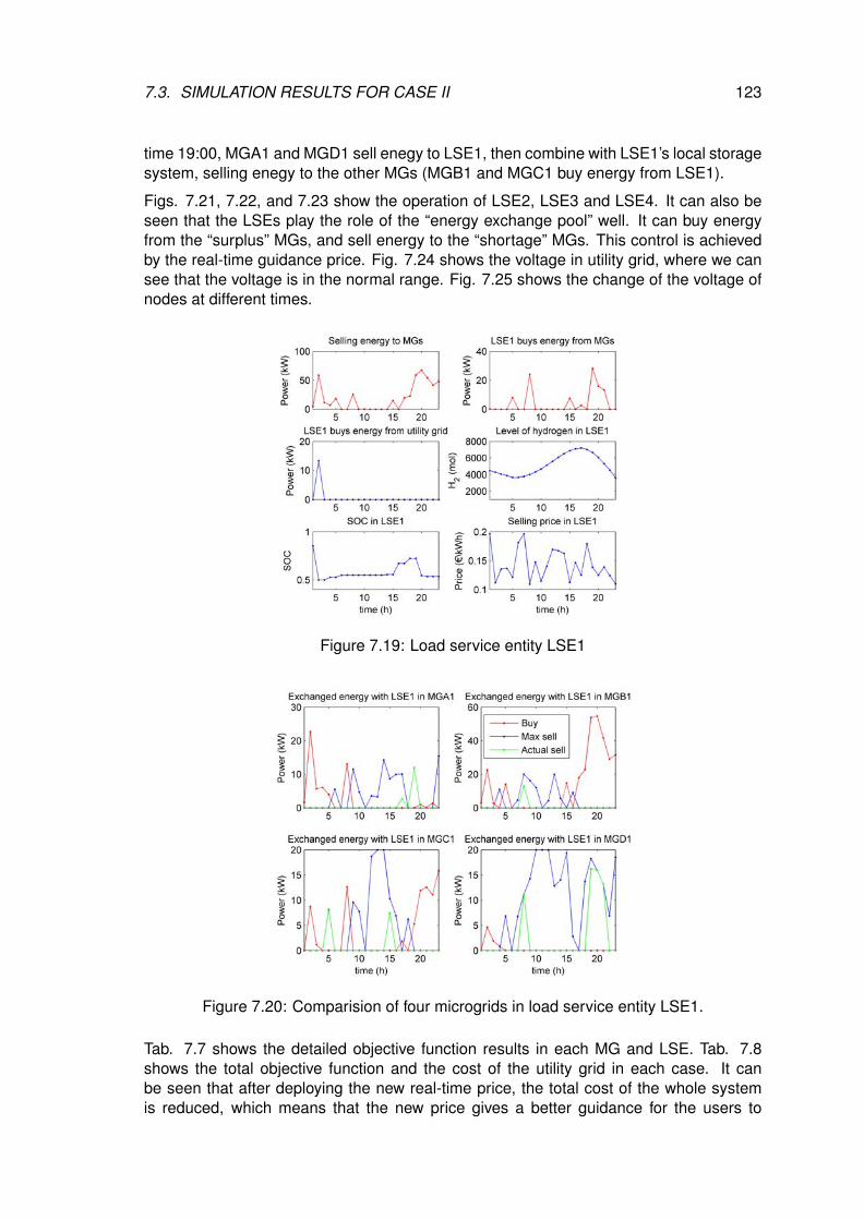
7.3. SIMULATION RESULTS FOR CASE II 123
time 19:00, MGA1 and MGD1 sell enegy to LSE1, then combine with LSE1’s local storagesystem, selling enegy to the other MGs (MGB1 and MGC1 buy energy from LSE1).
Figs. 7.21, 7.22, and 7.23 show the operation of LSE2, LSE3 and LSE4. It can also beseen that the LSEs play the role of the “energy exchange pool” well. It can buy energyfrom the “surplus” MGs, and sell energy to the “shortage” MGs. This control is achievedby the real-time guidance price. Fig. 7.24 shows the voltage in utility grid, where we cansee that the voltage is in the normal range. Fig. 7.25 shows the change of the voltage ofnodes at different times.
Figure 7.19: Load service entity LSE1
Figure 7.20: Comparision of four microgrids in load service entity LSE1.
Tab. 7.7 shows the detailed objective function results in each MG and LSE. Tab. 7.8shows the total objective function and the cost of the utility grid in each case. It canbe seen that after deploying the new real-time price, the total cost of the whole systemis reduced, which means that the new price gives a better guidance for the users to
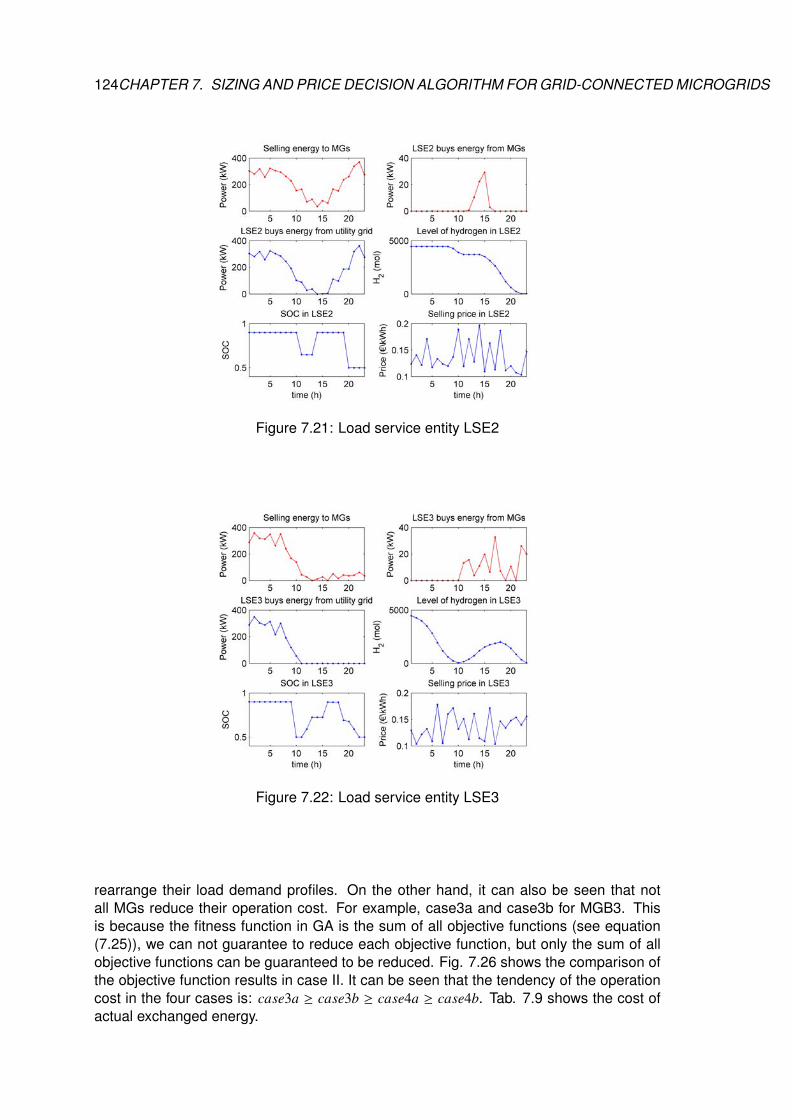
124CHAPTER 7. SIZING AND PRICE DECISION ALGORITHM FOR GRID-CONNECTED MICROGRIDS
Figure 7.21: Load service entity LSE2
Figure 7.22: Load service entity LSE3
rearrange their load demand profiles. On the other hand, it can also be seen that notall MGs reduce their operation cost. For example, case3a and case3b for MGB3. Thisis because the fitness function in GA is the sum of all objective functions (see equation(7.25)), we can not guarantee to reduce each objective function, but only the sum of allobjective functions can be guaranteed to be reduced. Fig. 7.26 shows the comparison ofthe objective function results in case II. It can be seen that the tendency of the operationcost in the four cases is: case3a ≥ case3b ≥ case4a ≥ case4b. Tab. 7.9 shows the cost ofactual exchanged energy.
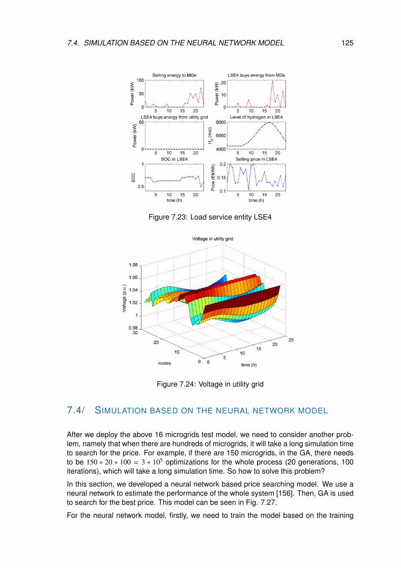
7.4. SIMULATION BASED ON THE NEURAL NETWORK MODEL 125
Figure 7.23: Load service entity LSE4
Figure 7.24: Voltage in utility grid
7.4/ SIMULATION BASED ON THE NEURAL NETWORK MODEL
After we deploy the above 16 microgrids test model, we need to consider another prob-lem, namely that when there are hundreds of microgrids, it will take a long simulation timeto search for the price. For example, if there are 150 microgrids, in the GA, there needsto be 150 ∗ 20 ∗ 100 = 3 ∗ 105 optimizations for the whole process (20 generations, 100iterations), which will take a long simulation time. So how to solve this problem?
In this section, we developed a neural network based price searching model. We use aneural network to estimate the performance of the whole system [156]. Then, GA is usedto search for the best price. This model can be seen in Fig. 7.27.
For the neural network model, firstly, we need to train the model based on the training
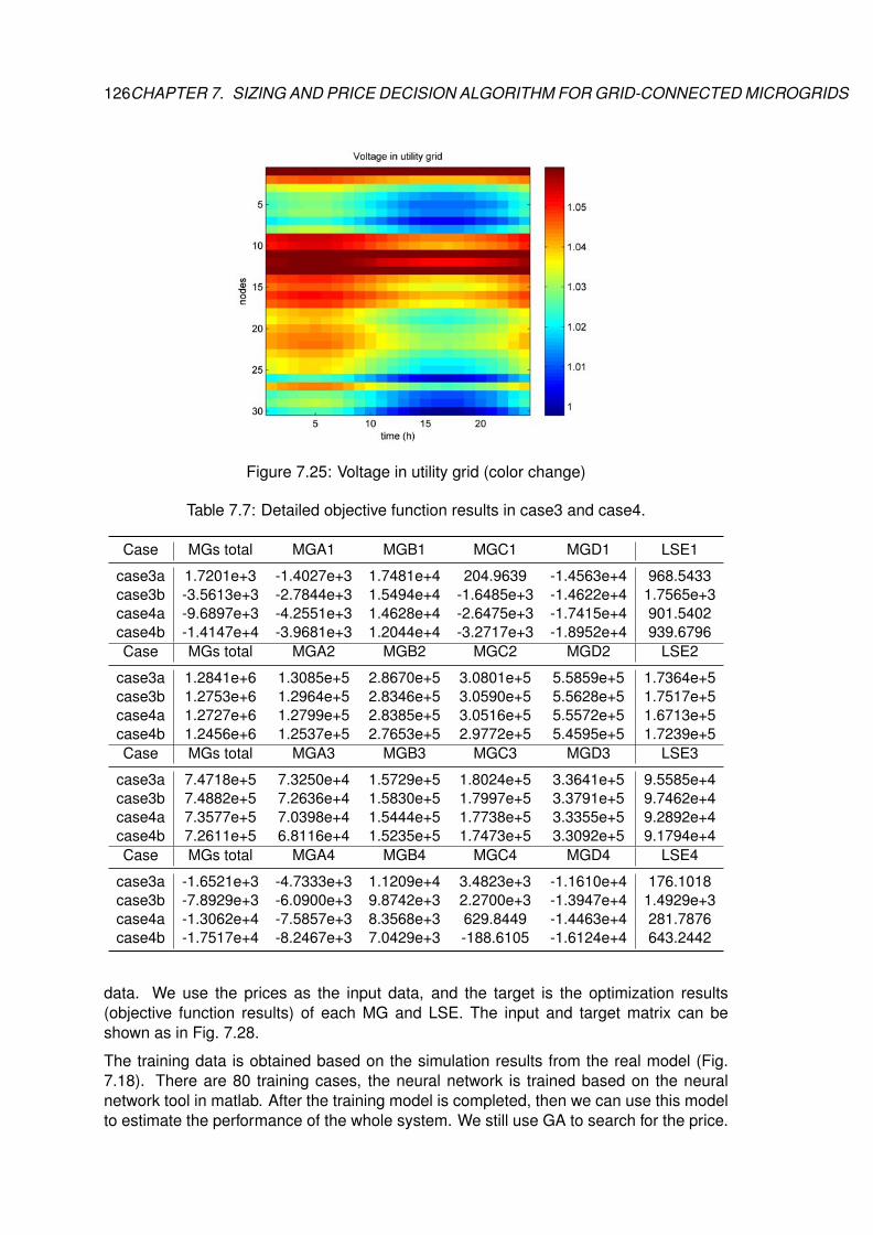
126CHAPTER 7. SIZING AND PRICE DECISION ALGORITHM FOR GRID-CONNECTED MICROGRIDS
Figure 7.25: Voltage in utility grid (color change)
Table 7.7: Detailed objective function results in case3 and case4.
Case MGs total MGA1 MGB1 MGC1 MGD1 LSE1
case3a 1.7201e+3 -1.4027e+3 1.7481e+4 204.9639 -1.4563e+4 968.5433case3b -3.5613e+3 -2.7844e+3 1.5494e+4 -1.6485e+3 -1.4622e+4 1.7565e+3case4a -9.6897e+3 -4.2551e+3 1.4628e+4 -2.6475e+3 -1.7415e+4 901.5402case4b -1.4147e+4 -3.9681e+3 1.2044e+4 -3.2717e+3 -1.8952e+4 939.6796Case MGs total MGA2 MGB2 MGC2 MGD2 LSE2
case3a 1.2841e+6 1.3085e+5 2.8670e+5 3.0801e+5 5.5859e+5 1.7364e+5case3b 1.2753e+6 1.2964e+5 2.8346e+5 3.0590e+5 5.5628e+5 1.7517e+5case4a 1.2727e+6 1.2799e+5 2.8385e+5 3.0516e+5 5.5572e+5 1.6713e+5case4b 1.2456e+6 1.2537e+5 2.7653e+5 2.9772e+5 5.4595e+5 1.7239e+5Case MGs total MGA3 MGB3 MGC3 MGD3 LSE3
case3a 7.4718e+5 7.3250e+4 1.5729e+5 1.8024e+5 3.3641e+5 9.5585e+4case3b 7.4882e+5 7.2636e+4 1.5830e+5 1.7997e+5 3.3791e+5 9.7462e+4case4a 7.3577e+5 7.0398e+4 1.5444e+5 1.7738e+5 3.3355e+5 9.2892e+4case4b 7.2611e+5 6.8116e+4 1.5235e+5 1.7473e+5 3.3092e+5 9.1794e+4Case MGs total MGA4 MGB4 MGC4 MGD4 LSE4
case3a -1.6521e+3 -4.7333e+3 1.1209e+4 3.4823e+3 -1.1610e+4 176.1018case3b -7.8929e+3 -6.0900e+3 9.8742e+3 2.2700e+3 -1.3947e+4 1.4929e+3case4a -1.3062e+4 -7.5857e+3 8.3568e+3 629.8449 -1.4463e+4 281.7876case4b -1.7517e+4 -8.2467e+3 7.0429e+3 -188.6105 -1.6124e+4 643.2442
data. We use the prices as the input data, and the target is the optimization results(objective function results) of each MG and LSE. The input and target matrix can beshown as in Fig. 7.28.
The training data is obtained based on the simulation results from the real model (Fig.7.18). There are 80 training cases, the neural network is trained based on the neuralnetwork tool in matlab. After the training model is completed, then we can use this modelto estimate the performance of the whole system. We still use GA to search for the price.
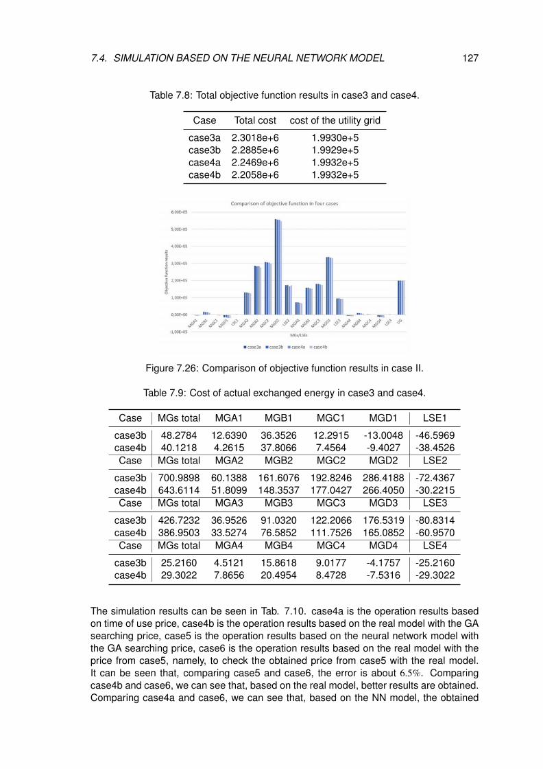
7.4. SIMULATION BASED ON THE NEURAL NETWORK MODEL 127
Table 7.8: Total objective function results in case3 and case4.
Case Total cost cost of the utility grid
case3a 2.3018e+6 1.9930e+5case3b 2.2885e+6 1.9929e+5case4a 2.2469e+6 1.9932e+5case4b 2.2058e+6 1.9932e+5
Figure 7.26: Comparison of objective function results in case II.
Table 7.9: Cost of actual exchanged energy in case3 and case4.
Case MGs total MGA1 MGB1 MGC1 MGD1 LSE1
case3b 48.2784 12.6390 36.3526 12.2915 -13.0048 -46.5969case4b 40.1218 4.2615 37.8066 7.4564 -9.4027 -38.4526Case MGs total MGA2 MGB2 MGC2 MGD2 LSE2
case3b 700.9898 60.1388 161.6076 192.8246 286.4188 -72.4367case4b 643.6114 51.8099 148.3537 177.0427 266.4050 -30.2215Case MGs total MGA3 MGB3 MGC3 MGD3 LSE3
case3b 426.7232 36.9526 91.0320 122.2066 176.5319 -80.8314case4b 386.9503 33.5274 76.5852 111.7526 165.0852 -60.9570Case MGs total MGA4 MGB4 MGC4 MGD4 LSE4
case3b 25.2160 4.5121 15.8618 9.0177 -4.1757 -25.2160case4b 29.3022 7.8656 20.4954 8.4728 -7.5316 -29.3022
The simulation results can be seen in Tab. 7.10. case4a is the operation results basedon time of use price, case4b is the operation results based on the real model with the GAsearching price, case5 is the operation results based on the neural network model withthe GA searching price, case6 is the operation results based on the real model with theprice from case5, namely, to check the obtained price from case5 with the real model.It can be seen that, comparing case5 and case6, the error is about 6.5%. Comparingcase4b and case6, we can see that, based on the real model, better results are obtained.Comparing case4a and case6, we can see that, based on the NN model, the obtained
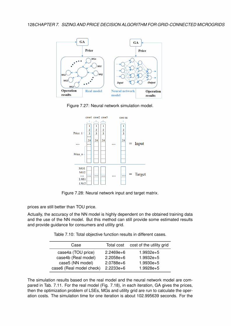
128CHAPTER 7. SIZING AND PRICE DECISION ALGORITHM FOR GRID-CONNECTED MICROGRIDS
Figure 7.27: Neural network simulation model.
Figure 7.28: Neural network input and target matrix.
prices are still better than TOU price.
Actually, the accuracy of the NN model is highly dependent on the obtained training dataand the use of the NN model. But this method can still provide some estimated resultsand provide guidance for consumers and utility grid.
Table 7.10: Total objective function results in different cases.
Case Total cost cost of the utility grid
case4a (TOU price) 2.2469e+6 1.9932e+5case4b (Real model) 2.2058e+6 1.9932e+5
case5 (NN model) 2.0788e+6 1.9930e+5case6 (Real model check) 2.2233e+6 1.9928e+5
The simulation results based on the real model and the neural network model are com-pared in Tab. 7.11. For the real model (Fig. 7.18), in each iteration, GA gives the prices,then the optimization problem of LSEs, MGs and utility grid are run to calculate the oper-ation costs. The simulation time for one iteration is about 102.995639 seconds. For the
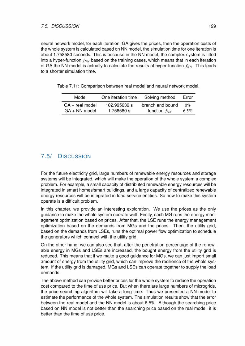
7.5. DISCUSSION 129
neural network model, for each iteration, GA gives the prices, then the operation costs ofthe whole system is calculated based on NN model, the simulation time for one iteration isabout 1.758580 seconds. This is because in the NN model, the complex system is fittedinto a hyper-function fNN based on the training cases, which means that in each iterationof GA,the NN model is actually to calculate the results of hyper-function fNN . This leadsto a shorter simulation time.
Table 7.11: Comparison between real model and neural network model.
Model One iteration time Solving method Error
GA + real model 102.995639 s branch and bound 0%GA + NN model 1.758580 s function fNN 6.5%
7.5/ DISCUSSION
For the future electricity grid, large numbers of renewable energy resources and storagesystems will be integrated, which will make the operation of the whole system a complexproblem. For example, a small capacity of distributed renewable energy resources will beintegrated in smart homes/smart buildings, and a large capacity of centralized renewableenergy resources will be integrated in load service entities. So how to make this systemoperate is a difficult problem.
In this chapter, we provide an interesting exploration. We use the prices as the onlyguidance to make the whole system operate well. Firstly, each MG runs the energy man-agement optimization based on prices. After that, the LSE runs the energy managementoptimization based on the demands from MGs and the prices. Then, the utility grid,based on the demands from LSEs, runs the optimal power flow optimization to schedulethe generators which connect with the utility grid.
On the other hand, we can also see that, after the penetration percentage of the renew-able energy in MGs and LSEs are increased, the bought energy from the utility grid isreduced. This means that if we make a good guidance for MGs, we can just import smallamount of energy from the utility grid, which can improve the resilience of the whole sys-tem. If the utility grid is damaged, MGs and LSEs can operate together to supply the loaddemands.
The above method can provide better prices for the whole system to reduce the operationcost compared to the time of use price. But when there are large numbers of microgrids,the price searching algorithm will take a long time. Thus we presented a NN model toestimate the performance of the whole system. The simulation results show that the errorbetween the real model and the NN model is about 6.5%. Although the searching pricebased on NN model is not better than the searching price based on the real model, it isbetter than the time of use price.
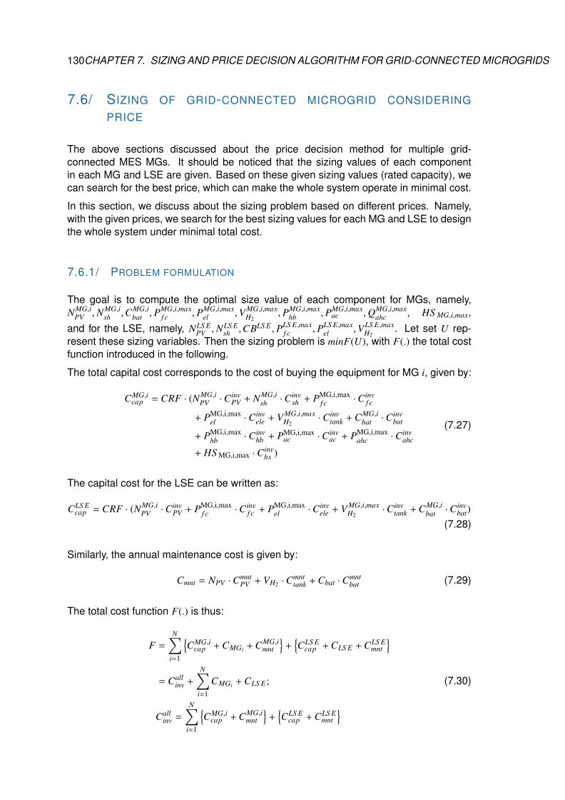
130CHAPTER 7. SIZING AND PRICE DECISION ALGORITHM FOR GRID-CONNECTED MICROGRIDS
7.6/ SIZING OF GRID-CONNECTED MICROGRID CONSIDERING
PRICE
The above sections discussed about the price decision method for multiple grid-connected MES MGs. It should be noticed that the sizing values of each componentin each MG and LSE are given. Based on these given sizing values (rated capacity), wecan search for the best price, which can make the whole system operate in minimal cost.
In this section, we discuss about the sizing problem based on different prices. Namely,with the given prices, we search for the best sizing values for each MG and LSE to designthe whole system under minimal total cost.
7.6.1/ PROBLEM FORMULATION
The goal is to compute the optimal size value of each component for MGs, namely,NMG,i
PV ,NMG,ish ,CMG,i
bat , PMG,i,maxf c , PMG,i,max
el ,V MG,i,maxH2
, PMG,i,maxhb , PMG,i,max
ac ,QMG,i,maxahc , HS MG,i,max,
and for the LSE, namely, NLS EPV ,NLS E
sh ,CBLS E , PLS E,maxf c , PLS E,max
el ,VLS E,maxH2
. Let set U rep-resent these sizing variables. Then the sizing problem is minF(U), with F(.) the total costfunction introduced in the following.
The total capital cost corresponds to the cost of buying the equipment for MG i, given by:
CMG,icap = CRF · (NMG,i
PV ·CinvPV + NMG,i
sh ·Cinvsh + PMG,i,max
f c ·Cinvf c
+ PMG,i,maxel ·Cinv
ele + V MG,i,maxH2
·Cinvtank + CMG,i
bat ·Cinvbat
+ PMG,i,maxhb ·Cinv
hb + PMG,i,maxac ·Cinv
ac + PMG,i,maxahc ·Cinv
ahc
+ HS MG,i,max ·Cinvhs )
(7.27)
The capital cost for the LSE can be written as:
CLS Ecap = CRF · (NMG,i
PV ·CinvPV + PMG,i,max
f c ·Cinvf c + PMG,i,max
el ·Cinvele + V MG,i,max
H2·Cinv
tank + CMG,ibat ·C
invbat)
(7.28)
Similarly, the annual maintenance cost is given by:
Cmnt = NPV ·CmntPV + VH2 ·C
mnttank + Cbat ·Cmnt
bat (7.29)
The total cost function F(.) is thus:
F =
N∑i=1
{CMG,i
cap + CMGi + CMG,imnt
}+
{CLS E
cap + CLS E + CLS Emnt
}= Call
inv +
N∑i=1
CMGi + CLS E;
Callinv =
N∑i=1
{CMG,i
cap + CMG,imnt
}+
{CLS E
cap + CLS Emnt
}(7.30)
7.6. SIZING OF GRID-CONNECTED MICROGRID CONSIDERING PRICE 131
Then the whole problem can be written as:
minU
Callinv +
N∑i=1
{min
U∗,price∗,exchCMGi
}+ min
U∗,price∗,∑N
i=1 exch∗iCLS E
s.t. (7.2), (7.3), (7.4), (7.5), (7.6), (7.7), (7.8), (7.13), (7.18), (7.19),
(7.20), (7.21), (7.23), (7.22), (7.24)
(7.31)
U∗ ∈ U is the best sizing values for each MG and LSE. price∗ is the given price. exch∗ ∈exch is the exchanged energy between MG and LSE.
This sizing problem can be described as: under the given price price∗, searching for thebest sizing values U∗ ∈ U which can make the whole system operate under minimal totalcost, and at the same time, ensure the energy exchange between MGs and LSE. It shouldbe pointed out that the price is a given parameter. This is because only with the givenprice, the energy flow in the whole system can be decided, then the sizing values can besearched.
The simulation flow chart can be seen in Fig. 7.29.
Figure 7.29: Flow chart for sizing problem considering price.
With the given sizing values from the GA algorithm, firstly, each MG runs its operationproblem (7.9). Then, the total bought energy Tbuy and sold energy Tsell are transferred tothe LSE. Next, the LSE runs its operation problem (7.1). After that, the fitness functions(total cost) 7.30 are calculated; and at last, GA updates the new population of sizingvalues. This process is repeated until the stopping criteria are satisfied.
7.6.2/ SIMULATION RESULTS
We take Case I as the example. In Case I, there are 4 MGs and 1 LSE. GA generates thesizing values for 4 MG and 1 LSE, there are 45 variables (10 components in each MG, 5components in the LSE). Two cases are compared:
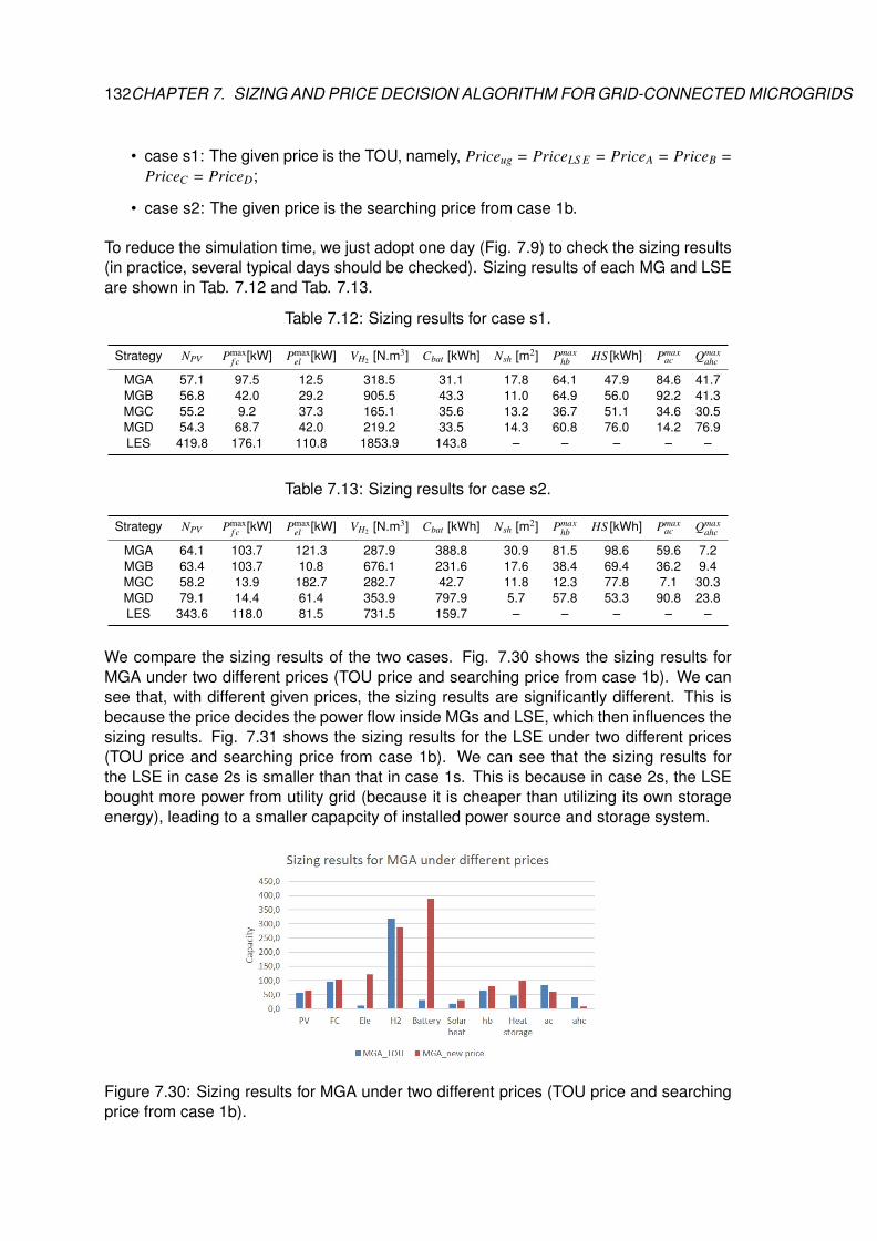
132CHAPTER 7. SIZING AND PRICE DECISION ALGORITHM FOR GRID-CONNECTED MICROGRIDS
• case s1: The given price is the TOU, namely, Priceug = PriceLS E = PriceA = PriceB =
PriceC = PriceD;
• case s2: The given price is the searching price from case 1b.
To reduce the simulation time, we just adopt one day (Fig. 7.9) to check the sizing results(in practice, several typical days should be checked). Sizing results of each MG and LSEare shown in Tab. 7.12 and Tab. 7.13.
Table 7.12: Sizing results for case s1.
Strategy NPV Pmaxf c [kW] Pmax
el [kW] VH2 [N.m3] Cbat [kWh] Nsh [m2] Pmaxhb HS [kWh] Pmax
ac Qmaxahc
MGA 57.1 97.5 12.5 318.5 31.1 17.8 64.1 47.9 84.6 41.7MGB 56.8 42.0 29.2 905.5 43.3 11.0 64.9 56.0 92.2 41.3MGC 55.2 9.2 37.3 165.1 35.6 13.2 36.7 51.1 34.6 30.5MGD 54.3 68.7 42.0 219.2 33.5 14.3 60.8 76.0 14.2 76.9LES 419.8 176.1 110.8 1853.9 143.8 – – – – –
Table 7.13: Sizing results for case s2.
Strategy NPV Pmaxf c [kW] Pmax
el [kW] VH2 [N.m3] Cbat [kWh] Nsh [m2] Pmaxhb HS [kWh] Pmax
ac Qmaxahc
MGA 64.1 103.7 121.3 287.9 388.8 30.9 81.5 98.6 59.6 7.2MGB 63.4 103.7 10.8 676.1 231.6 17.6 38.4 69.4 36.2 9.4MGC 58.2 13.9 182.7 282.7 42.7 11.8 12.3 77.8 7.1 30.3MGD 79.1 14.4 61.4 353.9 797.9 5.7 57.8 53.3 90.8 23.8LES 343.6 118.0 81.5 731.5 159.7 – – – – –
We compare the sizing results of the two cases. Fig. 7.30 shows the sizing results forMGA under two different prices (TOU price and searching price from case 1b). We cansee that, with different given prices, the sizing results are significantly different. This isbecause the price decides the power flow inside MGs and LSE, which then influences thesizing results. Fig. 7.31 shows the sizing results for the LSE under two different prices(TOU price and searching price from case 1b). We can see that the sizing results forthe LSE in case 2s is smaller than that in case 1s. This is because in case 2s, the LSEbought more power from utility grid (because it is cheaper than utilizing its own storageenergy), leading to a smaller capapcity of installed power source and storage system.
Figure 7.30: Sizing results for MGA under two different prices (TOU price and searchingprice from case 1b).
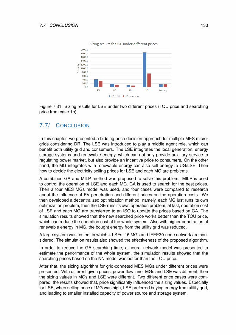
7.7. CONCLUSION 133
Figure 7.31: Sizing results for LSE under two different prices (TOU price and searchingprice from case 1b).
7.7/ CONCLUSION
In this chapter, we presented a bidding price decision approach for multiple MES micro-grids considering DR. The LSE was introduced to play a middle agent role, which canbenefit both utility grid and consumers. The LSE integrates the local generation, energystorage systems and renewable energy, which can not only provide auxiliary service toregulating power market, but also provide an incentive price to consumers. On the otherhand, the MG integrates with renewable energy can also sell energy to UG/LSE. Thenhow to decide the electricity selling prices for LSE and each MG are problems.
A combined GA and MILP method was proposed to solve this problem. MILP is usedto control the operation of LSE and each MG. GA is used to search for the best prices.Then a four MES MGs model was used, and four cases were compared to researchabout the influence of PV penetration and different prices on the operation costs. Wethen developed a decentralized optimization method, namely, each MG just runs its ownoptimization problem, then the LSE runs its own operation problem, at last, operation costof LSE and each MG are transferred to an ISO to update the prices based on GA. Thesimulation results showed that the new searched price works better than the TOU price,which can reduce the operation cost of the whole system. Also with higher penetration ofrenewable energy in MG, the bought energy from the utility grid was reduced.
A large system was tested, in which 4 LSEs, 16 MGs and IEEE30-node network are con-sidered. The simulation results also showed the effectiveness of the proposed algorithm.
In order to reduce the GA searching time, a neural network model was presented toestimate the performance of the whole system, the simulation results showed that thesearching prices based on the NN model was better than the TOU price.
After that, the sizing algorithm for grid-conneted MES MGs under different prices werepresented. With different given prices, power flow inner MGs and LSE was different, thenthe sizing values in MGs and LSE were different. Two different price cases were com-pared, the results showed that, price significantly influenced the sizing values. Especiallyfor LSE, when selling price of MG was high, LSE preferred buying energy from utility grid,and leading to smaller installed capacity of power source and storage system.


IIICONCLUSION
135

8CONCLUSION
This chapter is the conclusion of the whole dissertation. It discusses four aspects: 1) asummary of this dissertation; 2) the list of contributions; 3) the practical application of
the proposed co-optimization sizing method; and 4) future works.
8.1/ SUMMARY
In this dissertation, we focused on the sizing and operation problem of hydrogen-basedmicrogrids. We considered islanded microgrids (sections 4 and 5), and grid-connectedmicrogrids (section 6). Then we solved this problem while considering different specificaspects, including the operation strategy (2.2), the sizing method (2.3), the uncertainty onload demands (2.2.1), the degradation of energy storage system (5.3.4), and the resultsvalidation (4.3.8, 5.3.3). For grid-connected microgrids, we also considered the influenceof contingency events on the utility grid (sections 6.2.3, 6.3). Finally, a prices decisionapproach was also studied (section 7).
Firstly, for the operation strategies, we determined that three methods are often used:the rule-based strategy, the evolutionary algorithm, and the deterministic algorithm (suchas LP, MILP). We reviewed related operation strategies of microgrids in section 2.2. Inthis thesis, the MILP operation strategy was adopted to control the operation of microgridmodels.
Secondly, for the sizing method, the leader-follower (co-optimization) structure is oftenadopted. Related works about sizing methods was summarized in section 2.3. Theleader is typically the sizing problem, which uses a searching algorithm to search for thebest sizing values. The follower is the operation problem, which uses a deterministicalgorithm to solve the operation problem based on the sizing values from the leader. Inthis thesis, GA was used as the searching algorithm, and MILP was used to control theoperation of the microgrid, solved by a branch-and-bound algorithm.
Thirdly, for the uncertainty on the load demands and PV output, robust optimization wasadopted, namely, to find the worst and the best case based on the uncertainty level, whichis presented in section 2.2.1. The worst case (the case where the difference between thePV output and the load is the largest) is when the PV output is equal to the upper boundvalue, and the load is equal to the lower bound value. For the best case (the case wherethe difference between the PV output and the load is the lowest), when the PV output isequal to the lower bound value, the load is equal to the upper bound value.
137
138 CHAPTER 8. CONCLUSION
The degradation of the energy storage system was discussed in section 5.3.4. We consid-ered the degradation model of hydrogen storage system and the battery storage system.The simulation results showed that after we consider the degradation model, the sizingvalues were significantly influenced. We especially notice an increase in the capacity ofhydrogen storage and battery storage systems.
For the sizing results check, one-hour one-day rolling horizon optimization was adopted,as discussed in sections 4.3.8 and 5.3.3. As in the co-optimization, we often chooseseveral typical days to check whether sizing values are appropriate or not. We used rollinghorizon optimization to check these obtained results, and test whether there was anynecessary load shedding or curtailed power. In cases where these occured, adjustmentsto the sizing values were required.
Sixth, we looked at the influence of contingency events on the utility grid, as shown insections 6.2.3 and 6.3. We used the betweenness centrality index to describe the relativeimportance of each node for the whole system. Then we defined a worst case, namely,when the most important node was destroyed. We included the worst case in the sizingproblem to research about the influence of utility grid contingency events on the sizingvalues.
After that, for the price decision approach, we adopted the combined GA and MILPmethod to obtain the best prices to reduce the operation cost of the whole system, whichcan be found in section 7. MILP was used to control the operation of the microgrid andthe load service entity, and GA was used to search for the best price. At last, a neu-ral network was also developed to estimate the performance of the whole system andaccelerate computation time.
At last, a sizing algorithm for grid-connected MES MGs under different prices was pre-sented, as shown in section 7.6. With different given prices, power flow between MGs andLSE was different, and so the sizing values in MGs and LSE were different. Two differentprice cases were compared, and the results showed that price significantly influenced thesizing values.
8.2/ LIST OF CONTRIBUTIONS
Based on the previous elements, we list the main contributions of this thesis as follows:
1. A bi-level optimization method to perform microgrid sizing. A genetic algorithm isused to compute the sizing of the components to minimize the total annual cost(capital, maintenance and operation) of the system. Each candidate solution (set ofcomponents sizes) is evaluated with an MILP algorithm for scheduling validation;
2. A study on two types of microgrid architectures: a full-electric hydrogen-based mi-crogrid and a multi-energy supply hydrogen-based microgrid;
3. A model of the hydrogen storage system, integrating a degradation model for thefuel cell and the electrolyzer;
4. An MILP model to control energy flows, which considers technical and economiccriteria, such as the operation costs of the components, the startup costs of the fuelcell and the electrolyzer, the state-of-charge of the BSS, and the level-of-hydrogenof hydrogen tanks.
8.3. PRACTICAL APPLICATIONS 139
5. A 1-h resolution rolling-horizon simulation used to verify the validity of the obtainedsizing solutions, and to adjust the sizing values if required;
6. A multi-node gas/electricity/heat network model, where a hydrogen storage systemis used to keep the power balance;
7. In order to resist to contingency events, the use of betweenness centrality to findthe worst case under contingency events, and research about the influence of con-tingencies on the sizing results;
8. A decentralized price decision approach for UG-LSE-MGs, in which each MG andLSE runs its own operation problem;
9. A neural network model to estimate the performance (operation cost) of the wholesystem;
10. A sizing algorithm for grid-connected MES MGs under different prices is presented.
8.3/ PRACTICAL APPLICATIONS
In this section, we discuss how to use the proposed combined GA and MILP algorithm inpractical applications. It can be used in two aspects: the planning problem and the bilevelprice decision problem.
For the planning problem, we need to find the best values of each component to make thewhole system cost-effective. This is a non-convex combinational optimization problem,where we need to consider not only the long term planning period (such as 1 year), butalso the short term operation period (such as 1 hour), which makes the planning problemchallenging. Then we can use the presented combined planning algorithm, namely, usingGA to search for the sizing values, and the MILP (or the other operation strategy) tocontrol the operation of the whole system. After that, we can use the 1-hour one dayrolling horizon optimization to check the obtained sizing results, and to adjust the sizingvalues if required.
For the price decision problem. We need to consider both suppliers and consumers in-terests. The price is the link between suppliers and consumers. This is a bilevel problem,namely, the upper-level problem (the supplier operation is the upper-level problem) andthe lower-level problem (the MGs operation is the lower-level problem), which means thatprice is often the decision variable in the upper-level problem, and is treated as a pa-rameter in the lower-level problem. We can use the presented combined GA and MILPalgorithm to solve the price decision problem. GA is used to search for the prices, and theMILP is used to control the operation of suppliers and consumers. Based on this com-bined method, we can obtain the best prices, which can both benefit the energy suppliersand the consumers.
8.4/ FUTURE WORK
In this thesis, we have presented a combined GA and MILP algorithm to solve the plan-ning and price decision problem. But there are still many problems to be solved in thefuture, which can be concluded in as follows:
140 CHAPTER 8. CONCLUSION
1. The modeling of the hydrogen storage system. The consumed hydrogen of thefuel cell and produced hydrogen of electrolyzer will influence the sizing volume ofhydrogen tanks. In this thesis, we use a linear model to describe the consumedhydrogen of a fuel cell and the produced hydrogen of a electrolyzer. However, moreprecise models can be built, such as nonlinear models, which will be a future work;
2. The running time of the combined algorithm. Evolutionary algorithms need tosearch the “optimal” points in a large searching space, which makes the combinedalgorithm cost lots of time. Especially, when the inner operation problem is complexto solve, such as the MINLP operation problem, the whole simulation time will bevery long. Then, in the future, how to reduce the simulation time is a problem;
3. Other methods to solve the bilevel sizing problem. Two stage sizing optimizationproblem can be solved based on Benders decomposition method [157]. The innerproblem is the operation MILP problem, which can be transferred into a Lagrangedual problem. Solving the inner Lagrange dual problem, a Benders type cutting plancan be generated based on dual variables. Then, these Benders cuts are addedto the outer level problem. Using the Benders decomposition method to solve thesizing problem will be a future work;
4. The uncertainty of the load demands, renewable energy sources (such as PV, WT),and failure of power devices. In this thesis, we just consider the forecasted errorof the electricity load demands and PV generation, but actually, in the multi-energysupply microgrid, there are different types of load demands. This means that whenwe consider multiple forecasted error from different types of loads, the problem isharder to solve;
5. The artificial intelligence model to estimate the performance of the power systemintegrating large numbers of renewable energy resources. In the last sections ofthis thesis, we presented a neural network to estimate the performance of the IEEE30 network integrating microgrids. The error is about 6.5%, and how to reduce theerror will be researched in the future work.
BIBLIOGRAPHY
[1] WANG, Y., CHEN, C., WANG, J., AND BALDICK, R. Research on resilience ofpower systems under natural disasters-a review. IEEE Transactions on PowerSystems 31, 2 (2016), 1604–1613.
[2] CHEN, C., WANG, J., QIU, F., AND ZHAO, D. Resilient distribution system bymicrogrids formation after natural disasters. IEEE Transactions on Smart Grid7, 2 (March 2016), 958–966.
[3] CHEN, H., CONG, T. N., YANG, W., TAN, C., LI, Y., AND DING, Y. Progress inelectrical energy storage system: A critical review. Progress in Natural Science19, 3 (2009), 291–312.
[4] SHUKLA, A., AND PREM KUMAR, T. Nanostructured electrode materials for elec-trochemical energy storage and conversion. Wiley Interdisciplinary Reviews:Energy and Environment 2, 1 (2013), 14–30.
[5] JARAMILLO, L. B., AND WEIDLICH, A. Optimal microgrid scheduling with peakload reduction involving an electrolyzer and flexible loads. Applied Energy 169(2016), 857–865.
[6] KAZEMPOOR, P., DORER, V., AND OMMI, F. Evaluation of hydrogen andmethane-fuelled solid oxide fuel cell systems for residential applications:system design alternative and parameter study. international journal of hydro-gen energy 34, 20 (2009), 8630–8644.
[7] CAU, G., COCCO, D., PETROLLESE, M., KÆR, S. K., AND MILAN, C. Energymanagement strategy based on short-term generation scheduling for a re-newable microgrid using a hydrogen storage system. Energy Conversion andManagement 87 (2014), 820–831.
[8] WIKIPEDIA. Hydrogen production, 2018.
[9] BERTUCCIOLI, L., CHAN, A., HART, D., LEHNER, F., MADDEN, B., AND STANDEN,E. Development of water electrolysis in the european union. Fuel Cells andHydrogen Joint Undertaking (2014), 83.
[10] WIKIPEDIA. Fuel cell, 2018.
[11] DEPARTMENT OF ENERGY, U. fuel cells comparison, 2018.
[12] LIDULA, N., AND RAJAPAKSE, A. Microgrids research: A review of experimentalmicrogrids and test systems. Renewable and Sustainable Energy Reviews 15, 1(2011), 186–202.
[13] HATZIARGYRIOU, N., ASANO, H., IRAVANI, R., AND MARNAY, C. Microgrids. IEEEpower and energy magazine 5, 4 (2007), 78–94.
141
142 BIBLIOGRAPHY
[14] KATSIGIANNIS, Y. A., GEORGILAKIS, P. S., AND KARAPIDAKIS, E. S. Hybrid simu-lated annealing–tabu search method for optimal sizing of autonomous powersystems with renewables. IEEE Transactions on Sustainable Energy 3, 3 (2012),330–338.
[15] KYRIAKARAKOS, G., DOUNIS, A. I., ROZAKIS, S., ARVANITIS, K. G., AND PA-PADAKIS, G. Polygeneration microgrids: a viable solution in remote areas forsupplying power, potable water and hydrogen as transportation fuel. AppliedEnergy 88, 12 (2011), 4517–4526.
[16] ABBEY, C., CORNFORTH, D., HATZIARGYRIOU, N., HIROSE, K., KWASINSKI, A.,KYRIAKIDES, E., PLATT, G., REYES, L., AND SURYANARAYANAN, S. Poweringthrough the storm: microgrids operation for more efficient disaster recovery.IEEE power and energy magazine 12, 3 (2014), 67–76.
[17] AKHIL, A. A., HUFF, G., CURRIER, A. B., KAUN, B. C., RASTLER, D. M., CHEN,S. B., COTTER, A. L., BRADSHAW, D. T., AND GAUNTLETT, W. D. Electricitystorage handbook. Tech. rep., DOE/EPRI in collaboration with NRECA, 2013.
[18] KYRIAKARAKOS, G., PIROMALIS, D. D., ARVANITIS, K. G., DOUNIS, A. I., AND
PAPADAKIS, G. On battery-less autonomous polygeneration microgrids: In-vestigation of the combined hybrid capacitors/hydrogen alternative. EnergyConversion and Management 91 (2015), 405–415.
[19] LARMINIE, J., DICKS, A., AND MCDONALD, M. S. Fuel cell systems explained,vol. 2. Wiley New York, 2003.
[20] TESFAHUNEGN, S. G. Fuel cell assisted photovoltaic power systems.
[21] LAJNEF, T., ABID, S., AND AMMOUS, A. Modeling, control, and simulation ofa solar hydrogen/fuel cell hybrid energy system for grid-connected applica-tions. Advances in Power Electronics 2013 (2013).
[22] UZUNOGLU, M., ONAR, O., AND ALAM, M. Modeling, control and simulation of apv/fc/uc based hybrid power generation system for stand-alone applications.Renewable Energy 34, 3 (2009), 509–520.
[23] LIU, M., SHI, Y., AND FANG, F. Combined cooling, heating and power systems:A survey. Renewable and Sustainable Energy Reviews 35 (2014), 1–22.
[24] FACCI, A. L., CIGOLOTTI, V., JANNELLI, E., AND UBERTINI, S. Technical andeconomic assessment of a sofc-based energy system for combined cooling,heating and power. Applied Energy (2016).
[25] TSE, L. K. C., WILKINS, S., MCGLASHAN, N., URBAN, B., AND MARTINEZ-BOTAS,R. Solid oxide fuel cell/gas turbine trigeneration system for marine applica-tions. Journal of Power Sources 196, 6 (2011), 3149 – 3162.
[26] BANIASADI, E., AND ALEMRAJABI, A. A. Fuel cell energy generation and recov-ery cycle analysis for residential application. International Journal of HydrogenEnergy 35, 17 (2010), 9460 – 9467.
BIBLIOGRAPHY 143
[27] MENG, L., SANSEVERINO, E. R., LUNA, A., DRAGICEVIC, T., VASQUEZ, J. C., AND
GUERRERO, J. M. Microgrid supervisory controllers and energy managementsystems: A literature review. Renewable and Sustainable Energy Reviews 60(2016), 1263–1273.
[28] BAO, Z., ZHOU, Q., YANG, Z., YANG, Q., XU, L., AND WU, T. A multi time-scale and multi energy-type coordinated microgrid scheduling solution—parti: Model and methodology. IEEE Transactions on Power Systems 30, 5 (2015),2257–2266.
[29] LUO, Z., WU, Z., LI, Z., CAI, H., LI, B., AND GU, W. A two-stage optimizationand control for cchp microgrid energy management. Applied Thermal Engi-neering (2017).
[30] MASHAYEKH, S., STADLER, M., CARDOSO, G., AND HELENO, M. A mixed integerlinear programming approach for optimal der portfolio, sizing, and placementin multi-energy microgrids. Applied Energy 187 (2017), 154–168.
[31] MALEKI, A., AND ASKARZADEH, A. Comparative study of artificial intelligencetechniques for sizing of a hydrogen-based stand-alone photovoltaic/wind hy-brid system. international journal of hydrogen energy 39, 19 (2014), 9973–9984.
[32] MALEKI, A., AND POURFAYAZ, F. Optimal sizing of autonomous hybrid photo-voltaic/wind/battery power system with lpsp technology by using evolution-ary algorithms. Solar Energy 115 (2015), 471–483.
[33] FETANAT, A., AND KHORASANINEJAD, E. Size optimization for hybridphotovoltaic–wind energy system using ant colony optimization for contin-uous domains based integer programming. Applied Soft Computing 31 (2015),196–209.
[34] MALEKI, A., AND ASKARZADEH, A. Artificial bee swarm optimization for op-timum sizing of a stand-alone pv/wt/fc hybrid system considering lpsp con-cept. Solar Energy 107 (2014), 227–235.
[35] MALEKI, A., AMERI, M., AND KEYNIA, F. Scrutiny of multifarious particle swarmoptimization for finding the optimal size of a pv/wind/battery hybrid system.Renewable Energy 80 (2015), 552–563.
[36] ZHAO, B., ZHANG, X., LI, P., WANG, K., XUE, M., AND WANG, C. Optimal sizing,operating strategy and operational experience of a stand-alone microgrid ondongfushan island. Applied Energy 113 (2014), 1656–1666.
[37] ATIA, R., AND YAMADA, N. Optimization of a pv-wind-diesel system using ahybrid genetic algorithm. In Electrical Power and Energy Conference (EPEC),2012 IEEE (2012), IEEE, pp. 80–85.
[38] ROSS, M., HIDALGO, R., ABBEY, C., AND JOOS, G. Energy storage systemscheduling for an isolated microgrid. IET renewable power generation 5, 2(2011), 117–123.
[39] MARZBAND, M., PARHIZI, N., SAVAGHEBI, M., AND GUERRERO, J. M. Distributedsmart decision-making for a multimicrogrid system based on a hierarchicalinteractive architecture. IEEE Transactions on Energy Conversion 31, 2 (2016),637–648.
144 BIBLIOGRAPHY
[40] MARZBAND, M., AZARINEJADIAN, F., SAVAGHEBI, M., AND GUERRERO, J. M. Anoptimal energy management system for islanded microgrids based on mul-tiperiod artificial bee colony combined with markov chain. IEEE SYSTEMSJOURNAL (2015).
[41] MARZBAND, M., YOUSEFNEJAD, E., SUMPER, A., AND DOMINGUEZ-GARCIA, J. L.Real time experimental implementation of optimum energy management sys-tem in standalone microgrid by using multi-layer ant colony optimization. In-ternational Journal of Electrical Power & Energy Systems 75 (2016), 265–274.
[42] MURTY, P. Operation and control in power systems. BS Publications, 2011.
[43] HEMMATI, R., AND SABOORI, H. Short-term bulk energy storage systemscheduling for load leveling in unit commitment: modeling, optimization, andsensitivity analysis. Journal of advanced research 7, 3 (2016), 360–372.
[44] DETROJA, K. P. Optimal autonomous microgrid operation: A holistic view.Applied Energy 173 (2016), 320–330.
[45] GUO, L., LIU, W., CAI, J., HONG, B., AND WANG, C. A two-stage optimal plan-ning and design method for combined cooling, heat and power microgridsystem. Energy Conversion and Management 74 (2013), 433–445.
[46] KIM, J. S., AND EDGAR, T. F. Optimal scheduling of combined heat and powerplants using mixed-integer nonlinear programming. Energy 77 (2014), 675–690.
[47] MARZBAND, M., SUMPER, A., DOMINGUEZ-GARCIA, J. L., AND GUMARA-FERRET,R. Experimental validation of a real time energy management system formicrogrids in islanded mode using a local day-ahead electricity market andminlp. Energy Conversion and Management 76 (2013), 314–322.
[48] DANESHI, H., AND SRIVASTAVA, A. K. Security-constrained unit commitmentwith wind generation and compressed air energy storage. Generation, Trans-mission & Distribution, IET 6, 2 (2012), 167–175.
[49] PARHOUDEH, S., BAZIAR, A., MAZAREIE, A., AND KAVOUSI-FARD, A. A novelstochastic framework based on fuzzy cloud theory for modeling uncertaintyin the micro-grids. International Journal of Electrical Power & Energy Systems 80(2016), 73–80.
[50] ZAKARIAZADEH, A., JADID, S., AND SIANO, P. Smart microgrid energy and re-serve scheduling with demand response using stochastic optimization. Inter-national Journal of Electrical Power & Energy Systems 63 (2014), 523–533.
[51] XIANG, Y., LIU, J., AND LIU, Y. Robust energy management of microgrid withuncertain renewable generation and load. IEEE Transactions on Smart Grid 7,2 (2016), 1034–1043.
[52] KUZNETSOVA, E., LI, Y.-F., RUIZ, C., AND ZIO, E. An integrated frameworkof agent-based modelling and robust optimization for microgrid energy man-agement. Applied Energy 129 (2014), 70–88.
BIBLIOGRAPHY 145
[53] HUSSAIN, A., BUI, V.-H., AND KIM, H.-M. Robust optimization-based schedul-ing of multi-microgrids considering uncertainties. Energies 9, 4 (2016), 278.
[54] LIU, G., AND TOMSOVIC, K. Robust unit commitment considering uncertaindemand response. Electric Power Systems Research 119 (2015), 126–137.
[55] VALENCIA, F., COLLADO, J., SAEZ, D., AND MARIN, L. G. Robust energy man-agement system for a microgrid based on a fuzzy prediction interval model.IEEE Transactions on Smart Grid 7, 3 (2016), 1486–1494.
[56] JAYASEKARA, S., AND HALGAMUGE, S. A review on optimization strategies ofcombined cooling heating and power generation. In 2012 IEEE 6th Interna-tional Conference on Information and Automation for Sustainability (2012), IEEE,pp. 302–307.
[57] FANG, F., WANG, Q. H., AND SHI, Y. A novel optimal operational strategy forthe cchp system based on two operating modes. IEEE Transactions on PowerSystems 27, 2 (2012), 1032–1041.
[58] KAVVADIAS, K., TOSIOS, A., AND MAROULIS, Z. Design of a combined heating,cooling and power system: Sizing, operation strategy selection and paramet-ric analysis. Energy Conversion and Management 51, 4 (2010), 833–845.
[59] CHANG, L., WENG, G., HU, J., AND MAO, M. Operation and configuration op-timization of a cchp system for general building load. In Power Electronicsand Motion Control Conference (IPEMC-ECCE Asia), 2016 IEEE 8th International(2016), IEEE, pp. 1799–1805.
[60] KYRIAKARAKOS, G., PIROMALIS, D. D., DOUNIS, A. I., ARVANITIS, K. G., AND
PAPADAKIS, G. Intelligent demand side energy management system for au-tonomous polygeneration microgrids. Applied Energy 103 (2013), 39–51.
[61] MOHAMMADI-IVATLOO, B., MORADI-DALVAND, M., AND RABIEE, A. Combinedheat and power economic dispatch problem solution using particle swarmoptimization with time varying acceleration coefficients. Electric Power Sys-tems Research 95 (2013), 9–18.
[62] BASU, M. Artificial immune system for combined heat and power economicdispatch. International Journal of Electrical Power & Energy Systems 43, 1 (2012),1–5.
[63] MOTEVASEL, M., SEIFI, A. R., AND NIKNAM, T. Multi-objective energy manage-ment of chp (combined heat and power)-based micro-grid. Energy 51 (2013),123–136.
[64] PIPERAGKAS, G., ANASTASIADIS, A., AND HATZIARGYRIOU, N. Stochastic pso-based heat and power dispatch under environmental constraints incorporat-ing chp and wind power units. Electric Power Systems Research 81, 1 (2011),209–218.
[65] WEI, D., CHEN, A., SUN, B., AND ZHANG, C. Multi-objective optimal opera-tion and energy coupling analysis of combined cooling and heating system.Energy 98 (2016), 296–307.
146 BIBLIOGRAPHY
[66] BORNAPOUR, M., HOOSHMAND, R.-A., KHODABAKHSHIAN, A., AND PARASTE-GARI, M. Optimal stochastic coordinated scheduling of proton exchangemembrane fuel cell-combined heat and power, wind and photovoltaic unitsin micro grids considering hydrogen storage. Applied Energy 202 (2017), 308–322.
[67] CHEN, X., KANG, C., O’MALLEY, M., XIA, Q., BAI, J., LIU, C., SUN, R., WANG,W., AND LI, H. Increasing the flexibility of combined heat and power for windpower integration in china: Modeling and implications. IEEE Transactions onPower Systems 30, 4 (2015), 1848–1857.
[68] BISCHI, A., TACCARI, L., MARTELLI, E., AMALDI, E., MANZOLINI, G., SILVA, P.,CAMPANARI, S., AND MACCHI, E. A detailed milp optimization model for com-bined cooling, heat and power system operation planning. Energy 74 (2014),12–26.
[69] LOZANO, M. A., RAMOS, J. C., AND SERRA, L. M. Cost optimization of thedesign of chcp (combined heat, cooling and power) systems under legal con-straints. Energy 35, 2 (2010), 794–805.
[70] ARCURI, P., FLORIO, G., AND FRAGIACOMO, P. A mixed integer programmingmodel for optimal design of trigeneration in a hospital complex. Energy 32, 8(2007), 1430–1447.
[71] SACHS, J., AND SAWODNY, O. Multi-objective three stage design optimizationfor island microgrids. Applied Energy 165 (2016), 789–800.
[72] HOWARD, B., AND MODI, V. Examination of the optimal operation of buildingscale combined heat and power systems under disparate climate and ghgemissions rates. Applied Energy 185 (2017), 280–293.
[73] GUROBI. gurobi, 2018.
[74] ZHOU, W., LOU, C., LI, Z., LU, L., AND YANG, H. Current status of research onoptimum sizing of stand-alone hybrid solar–wind power generation systems.Applied Energy 87, 2 (2010), 380–389.
[75] CONNOLLY, D., LUND, H., MATHIESEN, B. V., AND LEAHY, M. A review of com-puter tools for analysing the integration of renewable energy into various en-ergy systems. Applied Energy 87, 4 (2010), 1059–1082.
[76] DUFO-LOPEZ, R., BERNAL-AGUSTIN, J. L., AND CONTRERAS, J. Optimization ofcontrol strategies for stand-alone renewable energy systems with hydrogenstorage. Renewable energy 32, 7 (2007), 1102–1126.
[77] KHODAEI, A., AND SHAHIDEHPOUR, M. Microgrid-based co-optimization of gen-eration and transmission planning in power systems. IEEE transactions onpower systems 28, 2 (2013), 1582–1590.
[78] KHODAEI, A., BAHRAMIRAD, S., AND SHAHIDEHPOUR, M. Microgrid planningunder uncertainty. IEEE Transactions on Power Systems 30, 5 (2015), 2417–2425.
BIBLIOGRAPHY 147
[79] ZHANG, J., LI, K.-J., WANG, M., LEE, W.-J., AND GAO, H. A bi-level program forthe planning of an islanded microgrid including caes. In Industry ApplicationsSociety Annual Meeting, 2015 IEEE (2015), IEEE, pp. 1–8.
[80] EBRAHIMI, M., AND KESHAVARZ, A. Climate impact on the prime mover sizeand design of a cchp system for the residential building. Energy and Buildings54 (2012), 283–289.
[81] RUAN, Y., LIU, Q., LI, Z., AND WU, J. Optimization and analysis of buildingcombined cooling, heating and power (bchp) plants with chilled ice thermalstorage system. Applied Energy 179 (2016), 738–754.
[82] BEIHONG, Z., AND WEIDING, L. An optimal sizing method for cogenerationplants. Energy and Buildings 38, 3 (2006), 189–195.
[83] SHANEB, O., COATES, G., AND TAYLOR, P. Sizing of residential µchp systems.Energy and Buildings 43, 8 (2011), 1991–2001.
[84] SANAYE, S., AND KHAKPAAY, N. Simultaneous use of mrm (maximum rectanglemethod) and optimization methods in determining nominal capacity of gasengines in cchp (combined cooling, heating and power) systems. Energy 72(2014), 145–158.
[85] WANG, J., SUI, J., AND JIN, H. An improved operation strategy of combinedcooling heating and power system following electrical load. Energy 85 (2015),654–666.
[86] WANG, J., LU, Y., YANG, Y., AND MAO, T. Thermodynamic performance analy-sis and optimization of a solar-assisted combined cooling, heating and powersystem. Energy 115 (2016), 49–59.
[87] ZHU, Q., LUO, X., ZHANG, B., AND CHEN, Y. Mathematical modelling and op-timization of a large-scale combined cooling, heat, and power system thatincorporates unit changeover and time-of-use electricity price. Energy Con-version and Management (2016).
[88] PRAKASH, P., AND KHATOD, D. K. Optimal sizing and siting techniques fordistributed generation in distribution systems: A review. Renewable and Sus-tainable Energy Reviews 57 (2016), 111–130.
[89] JORDEHI, A. R. Allocation of distributed generation units in electric powersystems: A review. Renewable and Sustainable Energy Reviews 56 (2016), 893–905.
[90] ROH, J. H., SHAHIDEHPOUR, M., AND FU, Y. Market-based coordination oftransmission and generation capacity planning. IEEE Transactions on PowerSystems 22, 4 (2007), 1406–1419.
[91] KHAYATIAN, A., BARATI, M., AND LIM, G. J. Market-based and resilient coordi-nated microgrid planning under uncertainty. In Transmission and DistributionConference and Exposition (T&D), 2016 IEEE/PES (2016), IEEE, pp. 1–5.
[92] HEMMATI, R., SABOORI, H., AND SIANO, P. Coordinated short-term schedul-ing and long-term expansion planning in microgrids incorporating renewableenergy resources and energy storage systems. Energy (2017).
148 BIBLIOGRAPHY
[93] YANG, Y., ZHANG, S., AND XIAO, Y. Optimal design of distributed energy re-source systems coupled with energy distribution networks. Energy 85 (2015),433–448.
[94] ZIDAN, A., GABBAR, H. A., AND ELDESSOUKY, A. Optimal planning of combinedheat and power systems within microgrids. Energy 93 (2015), 235–244.
[95] SHAO, C., SHAHIDEHPOUR, M., WANG, X., WANG, X., AND WANG, B. Integratedplanning of electricity and natural gas transportation systems for enhancingthe power grid resilience. IEEE Transactions on Power Systems (2017).
[96] ZHANG, X., SHAHIDEHPOUR, M., ALABDULWAHAB, A. S., AND ABUSORRAH, A.Security-constrained co-optimization planning of electricity and natural gastransportation infrastructures. IEEE Transactions on Power Systems 30, 6(2015), 2984–2993.
[97] QIU, J., DONG, Z. Y., ZHAO, J. H., MENG, K., ZHENG, Y., AND HILL, D. J. Lowcarbon oriented expansion planning of integrated gas and power systems.IEEE Transactions on Power Systems 30, 2 (2015), 1035–1046.
[98] UNSIHUAY-VILA, C., MARANGON-LIMA, J., DE SOUZA, A. Z., PEREZ-ARRIAGA,I. J., AND BALESTRASSI, P. P. A model to long-term, multiarea, multistage, andintegrated expansion planning of electricity and natural gas systems. IEEETransactions on Power Systems 25, 2 (2010), 1154–1168.
[99] YU, M., AND HONG, S. H. Supply–demand balancing for power managementin smart grid: A stackelberg game approach. Applied Energy 164 (2016), 702–710.
[100] REIHANI, E., MOTALLEB, M., THORNTON, M., AND GHORBANI, R. A novel ap-proach using flexible scheduling and aggregation to optimize demand re-sponse in the developing interactive grid market architecture. Applied Energy183 (2016), 445–455.
[101] TUSHAR, W., CHAI, B., YUEN, C., SMITH, D. B., WOOD, K. L., YANG, Z., AND
POOR, H. V. Three-party energy management with distributed energy re-sources in smart grid. IEEE Transactions on Industrial Electronics 62, 4 (2015),2487–2498.
[102] WANG, Y., AI, X., TAN, Z., YAN, L., AND LIU, S. Interactive dispatch modes andbidding strategy of multiple virtual power plants based on demand responseand game theory. IEEE Transactions on Smart Grid 7, 1 (2016), 510–519.
[103] BAHRAMI, S., AND SHEIKHI, A. From demand response in smart grid towardintegrated demand response in smart energy hub. IEEE Transactions on SmartGrid 7, 2 (2016), 650–658.
[104] KAMYAB, F., AMINI, M., SHEYKHHA, S., HASANPOUR, M., AND JALALI, M. M. De-mand response program in smart grid using supply function bidding mecha-nism. IEEE Transactions on Smart Grid 7, 3 (2016), 1277–1284.
[105] ZHONG, H., XIE, L., AND XIA, Q. Coupon incentive-based demand response:Theory and case study. IEEE Transactions on Power Systems 28, 2 (2013), 1266–1276.
BIBLIOGRAPHY 149
[106] FANG, X., HU, Q., LI, F., WANG, B., AND LI, Y. Coupon-based demand re-sponse considering wind power uncertainty: A strategic bidding model forload serving entities. IEEE Transactions on Power Systems 31, 2 (2016), 1025–1037.
[107] YU, M., AND HONG, S. H. Incentive-based demand response considering hier-archical electricity market: A stackelberg game approach. Applied Energy 203(2017), 267–279.
[108] DING, Y., PINEDA, S., NYENG, P., ØSTERGAARD, J., LARSEN, E. M., AND WU,Q. Real-time market concept architecture for ecogrid eu—a prototype foreuropean smart grids. IEEE Transactions on Smart Grid 4, 4 (2013), 2006–2016.
[109] MANSHADI, S. D., AND KHODAYAR, M. E. A hierarchical electricity market struc-ture for the smart grid paradigm. IEEE Transactions on Smart Grid 7, 4 (2016),1866–1875.
[110] NGUYEN, D. T., NGUYEN, H. T., AND LE, L. B. Dynamic pricing design for de-mand response integration in power distribution networks. IEEE Transactionson Power Systems 31, 5 (2016), 3457–3472.
[111] ZUGNO, M., MORALES, J. M., PINSON, P., AND MADSEN, H. A bilevel model forelectricity retailers’ participation in a demand response market environment.Energy Economics 36 (2013), 182–197.
[112] ZHANG, C., WANG, Q., WANG, J., KORPS, M., PINSON, P., ØSTERGAARD, J., AND
KHODAYAR, M. E. Trading strategies for distribution company with stochasticdistributed energy resources. Applied Energy 177 (2016), 625–635.
[113] WANG, Z., CHEN, B., WANG, J., BEGOVIC, M. M., AND CHEN, C. Coordinatedenergy management of networked microgrids in distribution systems. IEEETransactions on Smart Grid 6, 1 (2015), 45–53.
[114] JALALI, M., ZARE, K., AND SEYEDI, H. Strategic decision-making of distribu-tion network operator with multi-microgrids considering demand responseprogram. Energy 141 (2017), 1059–1071.
[115] XIE, M., JI, X., HU, X., CHENG, P., DU, Y., AND LIU, M. Autonomous optimizedeconomic dispatch of active distribution system with multi-microgrids. En-ergy (2018).
[116] TESFAHUNEGN, S. G. Fuel Cell Assisted PhotoVoltaic Power Systems. PhDthesis, 2012.
[117] LAZAAR, M., BOUADILA, S., KOOLI, S., AND FARHAT, A. Comparative study ofconventional and solar heating systems under tunnel tunisian greenhouses:Thermal performance and economic analysis. Solar Energy 120 (2015), 620–635.
[118] LAURENCELLE, F., CHAHINE, R., HAMELIN, J., AGBOSSOU, K., FOURNIER, M.,BOSE, T., AND LAPERRIERE, A. Characterization of a ballard mk5-e protonexchange membrane fuel cell stack. Fuel Cells 1, 1 (2001), 66–71.
150 BIBLIOGRAPHY
[119] SHABANI, B., ANDREWS, J., AND WATKINS, S. Energy and cost analysis of asolar-hydrogen combined heat and power system for remote power supplyusing a computer simulation. Solar Energy 84, 1 (2010), 144–155.
[120] LI, J., HU, Z., XU, L., OUYANG, M., FANG, C., HU, J., CHENG, S., PO, H., ZHANG,W., AND JIANG, H. Fuel cell system degradation analysis of a chinese plug-inhybrid fuel cell city bus. International Journal of Hydrogen Energy 41, 34 (2016),15295–15310.
[121] MAMAGHANI, A. H., NAJAFI, B., CASALEGNO, A., AND RINALDI, F. Predictivemodelling and adaptive long-term performance optimization of an ht-pem fuelcell based micro combined heat and power (chp) plant. Applied Energy (2016).
[122] PEI, P., AND CHEN, H. Main factors affecting the lifetime of proton exchangemembrane fuel cells in vehicle applications: A review. Applied Energy 125(2014), 60–75.
[123] DIEGUEZ, P., URSUA, A., SANCHIS, P., SOPENA, C., GUELBENZU, E., AND
GANDIA, L. Thermal performance of a commercial alkaline water electrolyzer:experimental study and mathematical modeling. international journal of hydro-gen energy 33, 24 (2008), 7338–7354.
[124] ULLEBERG, Ø. Modeling of advanced alkaline electrolyzers: a system simula-tion approach. International journal of hydrogen energy 28, 1 (2003), 21–33.
[125] TIETZ, F., SEBOLD, D., BRISSE, A., AND SCHEFOLD, J. Degradation phenomenain a solid oxide electrolysis cell after 9000 h of operation. Journal of PowerSources 223 (2013), 129–135.
[126] KRUGER, E., AND TRAN, Q. T. Minimal aging operating strategies for batteryenergy storage systems in photovoltaic applications. In PES Innovative SmartGrid Technologies Conference Europe (ISGT-Europe), 2016 IEEE (2016), IEEE,pp. 1–6.
[127] OMAR, N., MONEM, M. A., FIROUZ, Y., SALMINEN, J., SMEKENS, J., HEGAZY,O., GAULOUS, H., MULDER, G., VAN DEN BOSSCHE, P., COOSEMANS, T., AND
OTHERS. Lithium iron phosphate based battery–assessment of the aging pa-rameters and development of cycle life model. Applied Energy 113 (2014),1575–1585.
[128] XINWEI, S., YINGDUO, H., SHOUZHEN, Z., ZHENG, J., QINGSHENG, L., AND JING,N. Comprehensive power-supply planning for active distribution system con-sidering cooling, heating and power load balance. Journal of Modern PowerSystems and Clean Energy 3, 4 (2015), 485–493.
[129] MENON, R. P., PAOLONE, M., AND MARECHAL, F. Study of optimal design ofpolygeneration systems in optimal control strategies. Energy 55 (2013), 134–141.
[130] GARCIA, F., AND BORDONS, C. Optimal economic dispatch for renewable en-ergy microgrids with hybrid storage using model predictive control. In Indus-trial Electronics Society, IECON 2013-39th Annual Conference of the IEEE (2013),IEEE, pp. 7932–7937.
BIBLIOGRAPHY 151
[131] HANSEN, T. M., ROCHE, R., SURYANARAYANAN, S., MACIEJEWSKI, A. A., AND
SIEGEL, H. J. Heuristic optimization for an aggregator-based resource alloca-tion in the smart grid. IEEE Transactions on Smart Grid 6, 4 (2015), 1785–1794.
[132] ROCHE, R., SURYANARAYANAN, S., HANSEN, T. M., KILICCOTE, S., AND MIRAOUI,A. A multi-agent model and strategy for residential demand response coordi-nation. In PowerTech, 2015 IEEE Eindhoven (June 2015), pp. 1–6.
[133] FERRARI-TRECATE, G., GALLESTEY, E., LETIZIA, P., SPEDICATO, M., MORARI,M., AND ANTOINE, M. Modeling and control of co-generation power plants: ahybrid system approach. IEEE Transactions on Control Systems Technology 12,5 (2004), 694–705.
[134] COLSON, B., MARCOTTE, P., AND SAVARD, G. An overview of bilevel optimiza-tion. Annals of operations research 153, 1 (2007), 235–256.
[135] LAGORSE, J., PAIRE, D., AND MIRAOUI, A. Sizing optimization of a stand-alonestreet lighting system powered by a hybrid system using fuel cell, {PV} andbattery. Renewable Energy 34, 3 (2009), 683 – 691.
[136] CASTANEDA, M., CANO, A., JURADO, F., SANCHEZ, H., AND FERNANDEZ, L. M.Sizing optimization, dynamic modeling and energy management strategies ofa stand-alone pv/hydrogen/battery-based hybrid system. International journalof hydrogen energy 38, 10 (2013), 3830–3845.
[137] WU, D., AND WANG, R. Combined cooling, heating and power: a review.progress in energy and combustion science 32, 5 (2006), 459–495.
[138] GU, W., WU, Z., BO, R., LIU, W., ZHOU, G., CHEN, W., AND WU, Z. Modeling,planning and optimal energy management of combined cooling, heating andpower microgrid: A review. International Journal of Electrical Power & EnergySystems 54 (2014), 26–37.
[139] MANCARELLA, P. Mes (multi-energy systems): An overview of concepts andevaluation models. Energy 65 (2014), 1–17.
[140] LI, B., ROCHE, R., AND MIRAOUI, A. System resilience improvement usingmultiple energy supply systems under natural disasters. In Industrial Elec-tronics Society, IECON 2016-42nd Annual Conference of the IEEE (2016), IEEE,pp. 3912–3917.
[141] REN, H., GAO, W., AND RUAN, Y. Optimal sizing for residential chp system.Applied Thermal Engineering 28, 5 (2008), 514–523.
[142] LI, B., ROCHE, R., AND MIRAOUI, A. Microgrid sizing with combined evolution-ary algorithm and milp unit commitment. Applied Energy 188 (2017), 547–562.
[143] WESOFF, E. Update: Ionex has a 1 mw battery ready for the grid, epri issuesess rfi, 2011.
[144] CONTAINERS, S. High cube shipping containers, 2018.
[145] MITRA, J., VALLEM, M. R., AND SINGH, C. Optimal deployment of distributedgeneration using a reliability criterion. IEEE Transactions on Industry Applica-tions 52, 3 (2016), 1989–1997.
152 BIBLIOGRAPHY
[146] LI, B., ROCHE, R., PAIRE, D., AND MIRAOUI, A. Sizing of a stand-alone micro-grid considering electric power, cooling/heating, hydrogen loads and hydro-gen storage degradation. Applied Energy 205 (2017), 1244–1259.
[147] SHEIKHI, A., BAHRAMI, S., AND RANJBAR, A. M. An autonomous demandresponse program for electricity and natural gas networks in smart energyhubs. Energy 89 (2015), 490–499.
[148] ZENG, B., AND ZHAO, L. Solving two-stage robust optimization problems usinga column-and-constraint generation method. Operations Research Letters 41,5 (2013), 457–461.
[149] WANG, Z., CHEN, B., WANG, J., KIM, J., AND BEGOVIC, M. M. Robust optimiza-tion based optimal dg placement in microgrids. IEEE Transactions on SmartGrid 5, 5 (2014), 2173–2182.
[150] YUAN, W., WANG, J., QIU, F., CHEN, C., KANG, C., AND ZENG, B. Robustoptimization-based resilient distribution network planning against naturaldisasters. IEEE Transactions on Smart Grid 7, 6 (2016), 2817–2826.
[151] CHANDA, S., AND SRIVASTAVA, A. K. Defining and enabling resiliency of elec-tric distribution systems with multiple microgrids. IEEE Transactions on SmartGrid 7, 6 (2016), 2859–2868.
[152] LOFBERG, J. Automatic robust convex programming. Optimization methodsand software 27, 1 (2012), 115–129.
[153] SHABANPOUR-HAGHIGHI, A., AND SEIFI, A. R. Simultaneous integrated optimalenergy flow of electricity, gas, and heat. Energy Conversion and Management101 (2015), 579–591.
[154] DE WOLF, D., AND SMEERS, Y. The gas transmission problem solved by anextension of the simplex algorithm. Management Science 46, 11 (2000), 1454–1465.
[155] MARTINEZ-MARES, A., AND FUERTE-ESQUIVEL, C. R. A unified gas and powerflow analysis in natural gas and electricity coupled networks. IEEE Transac-tions on Power Systems 27, 4 (2012), 2156–2166.
[156] XIA, L., MA, Z., KOKOGIANNAKIS, G., WANG, Z., AND WANG, S. A model-baseddesign optimization strategy for ground source heat pump systems with in-tegrated photovoltaic thermal collectors. Applied Energy 214 (2018), 178–190.
[157] ZHAO, L., AND ZENG, B. Robust unit commitment problem with demand re-sponse and wind energy. In Power and Energy Society General Meeting, 2012IEEE (2012), IEEE, pp. 1–8.
LIST OF FIGURES
1.1 Power and energy density comparison of fuel cell, battery and capacitor [4]. 4
1.2 Microgrid structure. . . . . . . . . . . . . . . . . . . . . . . . . . . . . . . . . 4
1.3 Sizing values vs. Costs. . . . . . . . . . . . . . . . . . . . . . . . . . . . . . 6
2.1 Sizing and operation. . . . . . . . . . . . . . . . . . . . . . . . . . . . . . . . 13
2.2 Computation burden, operation error vs. time scale. . . . . . . . . . . . . . 13
3.1 Voltage/current characteristic of a fuel cell. . . . . . . . . . . . . . . . . . . 33
3.2 Voltage and power characteristic of a fuel cell stack. . . . . . . . . . . . . . 33
3.3 Relationship between output power and consumed hydrogen. . . . . . . . . 34
3.4 Voltage/current characteristic of a fuel cell after different operation durations. 34
3.5 Voltage and current characteristic of one electrolyzer stack. . . . . . . . . . 36
3.6 Relationship between input power and produced hydrogen. . . . . . . . . . 37
3.7 Voltage/current characteristic of an electrolyzer after different operation du-rations. . . . . . . . . . . . . . . . . . . . . . . . . . . . . . . . . . . . . . . 37
3.8 Remaining capacity of battery vs. number of cycles. . . . . . . . . . . . . . 39
4.1 Microgrid architecture. . . . . . . . . . . . . . . . . . . . . . . . . . . . . . . 41
4.2 Bi-level optimization framework. . . . . . . . . . . . . . . . . . . . . . . . . . 42
4.3 Optimization process outline. . . . . . . . . . . . . . . . . . . . . . . . . . . 47
4.4 Weekly average solar radiation and load profiles. . . . . . . . . . . . . . . . 48
4.5 GA searching results for Case 1A. . . . . . . . . . . . . . . . . . . . . . . . 51
4.6 Scheduling results for Case 1A. The curve labelled “Power” corresponds tothe PV output minus the load. . . . . . . . . . . . . . . . . . . . . . . . . . . 51
4.7 LOH and SOC for Case 1A. . . . . . . . . . . . . . . . . . . . . . . . . . . . 52
4.8 LOH and SOC for Case 1B. . . . . . . . . . . . . . . . . . . . . . . . . . . . 52
4.9 Scheduling results for Case 2A. The curve labelled “Power” corresponds tothe PV output minus the load. . . . . . . . . . . . . . . . . . . . . . . . . . . 53
4.10 LOH and SOC for Case 2A. . . . . . . . . . . . . . . . . . . . . . . . . . . . 53
4.11 LOH and SOC for Case 2B. . . . . . . . . . . . . . . . . . . . . . . . . . . . 54
4.12 Load shedding vs. α & β. . . . . . . . . . . . . . . . . . . . . . . . . . . . . 54
153
154 LIST OF FIGURES
4.13 Curtailed power vs. α & β. . . . . . . . . . . . . . . . . . . . . . . . . . . . . 55
4.14 Scheduling results for Case 3. The curve labelled “Power” corresponds tothe PV output minus the load. . . . . . . . . . . . . . . . . . . . . . . . . . . 56
4.15 Shed and curtailed power, LOH and SOC profiles for Case 3. . . . . . . . . 56
4.16 Comparison of costs for all cases. . . . . . . . . . . . . . . . . . . . . . . . 57
4.17 Rule-based strategy algorithm. . . . . . . . . . . . . . . . . . . . . . . . . . 57
4.18 One-hour one-day rolling horizon scheduling simulation. . . . . . . . . . . . 58
4.19 One-hour one-day rolling horizon scheduling simulation (2000 h-2300 h).The curve labelled “Power” corresponds to the PV output minus the load. . 58
4.20 PV output minus load demand. . . . . . . . . . . . . . . . . . . . . . . . . . 59
4.21 One-hour one-day rolling horizon scheduling simulation with the new sizingvalue of HSS. . . . . . . . . . . . . . . . . . . . . . . . . . . . . . . . . . . . 59
4.22 One-hour one-day rolling horizon scheduling simulation with the new sizingvalue of HSS (2000 h-2300 h). The curve labelled “Power” corresponds tothe PV output minus the load. . . . . . . . . . . . . . . . . . . . . . . . . . . 60
4.23 Difference between PV output and load demand in 4 cases. . . . . . . . . . 60
5.1 Multi-energy supply microgrid structure. . . . . . . . . . . . . . . . . . . . . 64
5.2 Optimization process outline. . . . . . . . . . . . . . . . . . . . . . . . . . . 68
5.3 Cooling/heat/electricity/hydrogen demand (1 hour). . . . . . . . . . . . . . . 70
5.4 Solar radiation (1 hour). . . . . . . . . . . . . . . . . . . . . . . . . . . . . . 71
5.5 Cooling/heat/electricity/hydrogen demand (one day average). . . . . . . . . 71
5.6 Solar radiation (one day average). . . . . . . . . . . . . . . . . . . . . . . . 72
5.7 Strategy S2, electric power schedule (Power means PV outputs minuselectricity load demand; charge/discharge curves are for the battery). . . . 73
5.8 Strategy S2, heating power schedule (Power means solar outputs minusheat load demand; charge/discharge curves are for the heat storage sys-tem). . . . . . . . . . . . . . . . . . . . . . . . . . . . . . . . . . . . . . . . 74
5.9 Strategy S2, cooling power schedule. . . . . . . . . . . . . . . . . . . . . . 74
5.10 LOH and stored heat. . . . . . . . . . . . . . . . . . . . . . . . . . . . . . . 75
5.11 LOH and SOC. . . . . . . . . . . . . . . . . . . . . . . . . . . . . . . . . . . 75
5.12 1-hour rolling horizon simulation. . . . . . . . . . . . . . . . . . . . . . . . . 76
5.13 1-hour rolling horizon simulation, electric power schedule (2000-2168h). . . 76
5.14 1-hour rolling horizon simulation, heat power schedule (2000-2168h). . . . 77
5.15 1-hour rolling horizon simulation, cooling power schedule (2000-2168h). . . 77
5.16 1-hour rolling horizon simulation. . . . . . . . . . . . . . . . . . . . . . . . . 78
5.17 PV output minus load demand . . . . . . . . . . . . . . . . . . . . . . . . . 79
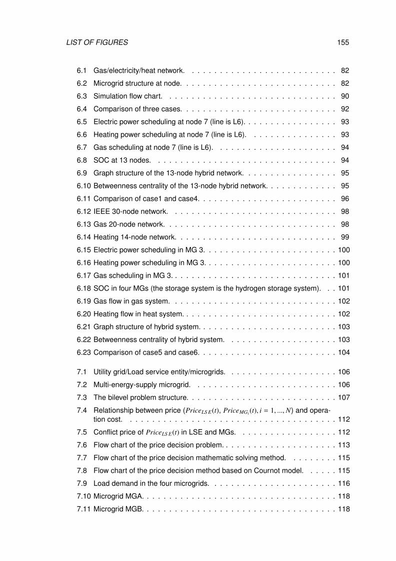
LIST OF FIGURES 155
6.1 Gas/electricity/heat network. . . . . . . . . . . . . . . . . . . . . . . . . . . 82
6.2 Microgrid structure at node. . . . . . . . . . . . . . . . . . . . . . . . . . . . 82
6.3 Simulation flow chart. . . . . . . . . . . . . . . . . . . . . . . . . . . . . . . 90
6.4 Comparison of three cases. . . . . . . . . . . . . . . . . . . . . . . . . . . . 92
6.5 Electric power scheduling at node 7 (line is L6). . . . . . . . . . . . . . . . . 93
6.6 Heating power scheduling at node 7 (line is L6). . . . . . . . . . . . . . . . 93
6.7 Gas scheduling at node 7 (line is L6). . . . . . . . . . . . . . . . . . . . . . 94
6.8 SOC at 13 nodes. . . . . . . . . . . . . . . . . . . . . . . . . . . . . . . . . 94
6.9 Graph structure of the 13-node hybrid network. . . . . . . . . . . . . . . . . 95
6.10 Betweenness centrality of the 13-node hybrid network. . . . . . . . . . . . . 95
6.11 Comparison of case1 and case4. . . . . . . . . . . . . . . . . . . . . . . . . 96
6.12 IEEE 30-node network. . . . . . . . . . . . . . . . . . . . . . . . . . . . . . 98
6.13 Gas 20-node network. . . . . . . . . . . . . . . . . . . . . . . . . . . . . . . 98
6.14 Heating 14-node network. . . . . . . . . . . . . . . . . . . . . . . . . . . . . 99
6.15 Electric power scheduling in MG 3. . . . . . . . . . . . . . . . . . . . . . . . 100
6.16 Heating power scheduling in MG 3. . . . . . . . . . . . . . . . . . . . . . . . 100
6.17 Gas scheduling in MG 3. . . . . . . . . . . . . . . . . . . . . . . . . . . . . . 101
6.18 SOC in four MGs (the storage system is the hydrogen storage system). . . 101
6.19 Gas flow in gas system. . . . . . . . . . . . . . . . . . . . . . . . . . . . . . 102
6.20 Heating flow in heat system. . . . . . . . . . . . . . . . . . . . . . . . . . . . 102
6.21 Graph structure of hybrid system. . . . . . . . . . . . . . . . . . . . . . . . . 103
6.22 Betweenness centrality of hybrid system. . . . . . . . . . . . . . . . . . . . 103
6.23 Comparison of case5 and case6. . . . . . . . . . . . . . . . . . . . . . . . . 104
7.1 Utility grid/Load service entity/microgrids. . . . . . . . . . . . . . . . . . . . 106
7.2 Multi-energy-supply microgrid. . . . . . . . . . . . . . . . . . . . . . . . . . 106
7.3 The bilevel problem structure. . . . . . . . . . . . . . . . . . . . . . . . . . . 107
7.4 Relationship between price (PriceLS E(t), PriceMGi(t), i = 1, ...,N) and opera-tion cost. . . . . . . . . . . . . . . . . . . . . . . . . . . . . . . . . . . . . . 112
7.5 Conflict price of PriceLS E(t) in LSE and MGs. . . . . . . . . . . . . . . . . . 112
7.6 Flow chart of the price decision problem. . . . . . . . . . . . . . . . . . . . . 113
7.7 Flow chart of the price decision mathematic solving method. . . . . . . . . 115
7.8 Flow chart of the price decision method based on Cournot model. . . . . . 115
7.9 Load demand in the four microgrids. . . . . . . . . . . . . . . . . . . . . . . 116
7.10 Microgrid MGA. . . . . . . . . . . . . . . . . . . . . . . . . . . . . . . . . . . 118
7.11 Microgrid MGB. . . . . . . . . . . . . . . . . . . . . . . . . . . . . . . . . . . 118
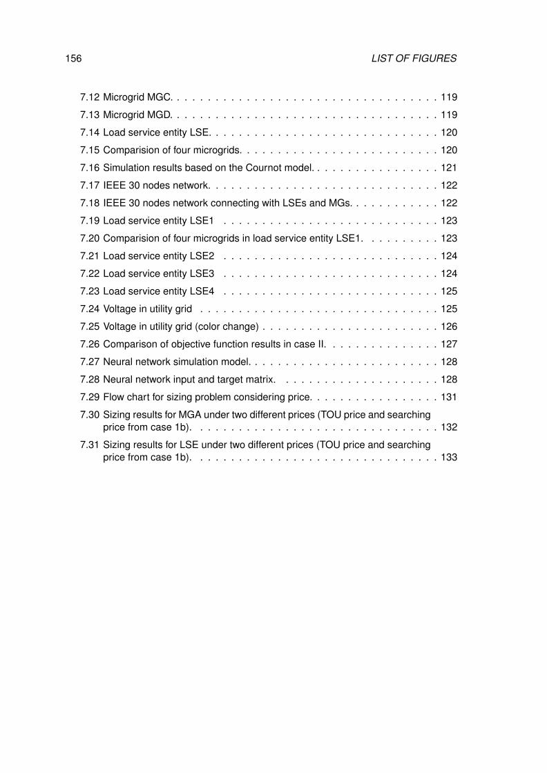
156 LIST OF FIGURES
7.12 Microgrid MGC. . . . . . . . . . . . . . . . . . . . . . . . . . . . . . . . . . . 119
7.13 Microgrid MGD. . . . . . . . . . . . . . . . . . . . . . . . . . . . . . . . . . . 119
7.14 Load service entity LSE. . . . . . . . . . . . . . . . . . . . . . . . . . . . . . 120
7.15 Comparision of four microgrids. . . . . . . . . . . . . . . . . . . . . . . . . . 120
7.16 Simulation results based on the Cournot model. . . . . . . . . . . . . . . . . 121
7.17 IEEE 30 nodes network. . . . . . . . . . . . . . . . . . . . . . . . . . . . . . 122
7.18 IEEE 30 nodes network connecting with LSEs and MGs. . . . . . . . . . . . 122
7.19 Load service entity LSE1 . . . . . . . . . . . . . . . . . . . . . . . . . . . . 123
7.20 Comparision of four microgrids in load service entity LSE1. . . . . . . . . . 123
7.21 Load service entity LSE2 . . . . . . . . . . . . . . . . . . . . . . . . . . . . 124
7.22 Load service entity LSE3 . . . . . . . . . . . . . . . . . . . . . . . . . . . . 124
7.23 Load service entity LSE4 . . . . . . . . . . . . . . . . . . . . . . . . . . . . 125
7.24 Voltage in utility grid . . . . . . . . . . . . . . . . . . . . . . . . . . . . . . . 125
7.25 Voltage in utility grid (color change) . . . . . . . . . . . . . . . . . . . . . . . 126
7.26 Comparison of objective function results in case II. . . . . . . . . . . . . . . 127
7.27 Neural network simulation model. . . . . . . . . . . . . . . . . . . . . . . . . 128
7.28 Neural network input and target matrix. . . . . . . . . . . . . . . . . . . . . 128
7.29 Flow chart for sizing problem considering price. . . . . . . . . . . . . . . . . 131
7.30 Sizing results for MGA under two different prices (TOU price and searchingprice from case 1b). . . . . . . . . . . . . . . . . . . . . . . . . . . . . . . . 132
7.31 Sizing results for LSE under two different prices (TOU price and searchingprice from case 1b). . . . . . . . . . . . . . . . . . . . . . . . . . . . . . . . 133
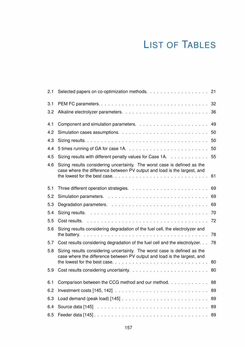
LIST OF TABLES
2.1 Selected papers on co-optimization methods. . . . . . . . . . . . . . . . . . 21
3.1 PEM FC parameters. . . . . . . . . . . . . . . . . . . . . . . . . . . . . . . . 32
3.2 Alkaline electrolyzer parameters. . . . . . . . . . . . . . . . . . . . . . . . . 36
4.1 Component and simulation parameters. . . . . . . . . . . . . . . . . . . . . 49
4.2 Simulation cases assumptions. . . . . . . . . . . . . . . . . . . . . . . . . . 50
4.3 Sizing results. . . . . . . . . . . . . . . . . . . . . . . . . . . . . . . . . . . . 50
4.4 5 times running of GA for case 1A. . . . . . . . . . . . . . . . . . . . . . . . 50
4.5 Sizing results with different penalty values for Case 1A. . . . . . . . . . . . 55
4.6 Sizing results considering uncertainty. The worst case is defined as thecase where the difference between PV output and load is the largest, andthe lowest for the best case. . . . . . . . . . . . . . . . . . . . . . . . . . . . 61
5.1 Three different operation strategies. . . . . . . . . . . . . . . . . . . . . . . 69
5.2 Simulation parameters. . . . . . . . . . . . . . . . . . . . . . . . . . . . . . 69
5.3 Degradation parameters. . . . . . . . . . . . . . . . . . . . . . . . . . . . . 69
5.4 Sizing results. . . . . . . . . . . . . . . . . . . . . . . . . . . . . . . . . . . 70
5.5 Cost results. . . . . . . . . . . . . . . . . . . . . . . . . . . . . . . . . . . . 72
5.6 Sizing results considering degradation of the fuel cell, the electrolyzer andthe battery. . . . . . . . . . . . . . . . . . . . . . . . . . . . . . . . . . . . . 78
5.7 Cost results considering degradation of the fuel cell and the electrolyzer. . . 78
5.8 Sizing results considering uncertainty. The worst case is defined as thecase where the difference between PV output and load is the largest, andthe lowest for the best case. . . . . . . . . . . . . . . . . . . . . . . . . . . . 80
5.9 Cost results considering uncertainty. . . . . . . . . . . . . . . . . . . . . . . 80
6.1 Comparison between the CCG method and our method. . . . . . . . . . . . 88
6.2 Investment costs [145, 142] . . . . . . . . . . . . . . . . . . . . . . . . . . . 89
6.3 Load demand (peak load) [145] . . . . . . . . . . . . . . . . . . . . . . . . . 89
6.4 Source data [145] . . . . . . . . . . . . . . . . . . . . . . . . . . . . . . . . 89
6.5 Feeder data [145] . . . . . . . . . . . . . . . . . . . . . . . . . . . . . . . . . 89
157
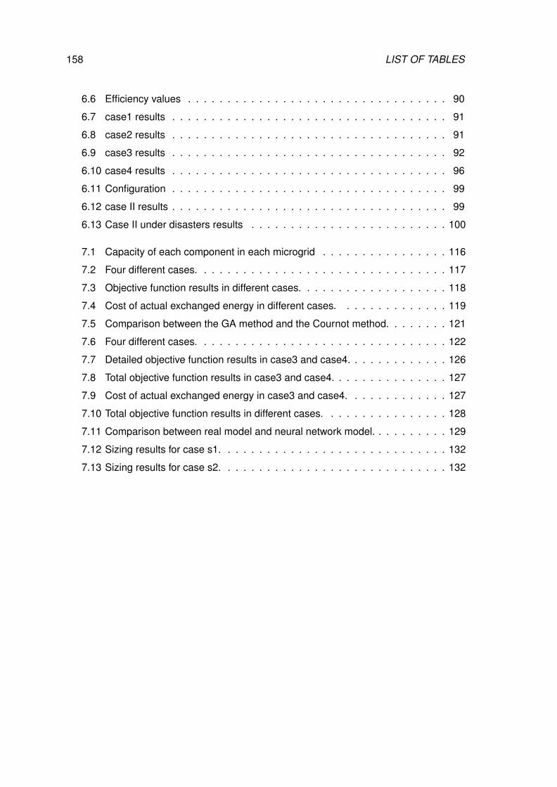
158 LIST OF TABLES
6.6 Efficiency values . . . . . . . . . . . . . . . . . . . . . . . . . . . . . . . . . 90
6.7 case1 results . . . . . . . . . . . . . . . . . . . . . . . . . . . . . . . . . . . 91
6.8 case2 results . . . . . . . . . . . . . . . . . . . . . . . . . . . . . . . . . . . 91
6.9 case3 results . . . . . . . . . . . . . . . . . . . . . . . . . . . . . . . . . . . 92
6.10 case4 results . . . . . . . . . . . . . . . . . . . . . . . . . . . . . . . . . . . 96
6.11 Configuration . . . . . . . . . . . . . . . . . . . . . . . . . . . . . . . . . . . 99
6.12 case II results . . . . . . . . . . . . . . . . . . . . . . . . . . . . . . . . . . . 99
6.13 Case II under disasters results . . . . . . . . . . . . . . . . . . . . . . . . . 100
7.1 Capacity of each component in each microgrid . . . . . . . . . . . . . . . . 116
7.2 Four different cases. . . . . . . . . . . . . . . . . . . . . . . . . . . . . . . . 117
7.3 Objective function results in different cases. . . . . . . . . . . . . . . . . . . 118
7.4 Cost of actual exchanged energy in different cases. . . . . . . . . . . . . . 119
7.5 Comparison between the GA method and the Cournot method. . . . . . . . 121
7.6 Four different cases. . . . . . . . . . . . . . . . . . . . . . . . . . . . . . . . 122
7.7 Detailed objective function results in case3 and case4. . . . . . . . . . . . . 126
7.8 Total objective function results in case3 and case4. . . . . . . . . . . . . . . 127
7.9 Cost of actual exchanged energy in case3 and case4. . . . . . . . . . . . . 127
7.10 Total objective function results in different cases. . . . . . . . . . . . . . . . 128
7.11 Comparison between real model and neural network model. . . . . . . . . . 129
7.12 Sizing results for case s1. . . . . . . . . . . . . . . . . . . . . . . . . . . . . 132
7.13 Sizing results for case s2. . . . . . . . . . . . . . . . . . . . . . . . . . . . . 132

IVAPPENDIX
159

ALIST OF PUBLICATIONS BY THE
AUTHOR
Journal:
• Li Bei, Robin Roche, and Abdellatif Miraoui. “Microgrid sizing with combined evolu-tionary algorithm and MILP unit commitment.” Applied energy 188 (2017): 547-562.
• Li Bei, Robin Roche, Damien Paire, and Abdellatif Miraoui. “Sizing of a stand-alonemicrogrid considering electric power, cooling/heating, hydrogen loads and hydrogenstorage degradation.” Applied Energy 205 (2017): 1244-1259.
• Li Bei, Robin Roche, Damien Paire, and Abdellatif Miraoui. “Optimal sizing of dis-tributed generation in gas/electricity/heat supply networks.” Energy 151 (2018): 675-688.
Conference:
• Li Bei, Robin Roche, Damien Paire, and Abdellatif Miraoui. “A price decision ap-proach for multiple multi-energy-supply microgrids considering demand response.”In EnergyCon, 2018 IEEE Cyprus. IEEE, 2018.
• Li Bei, Robin Roche, and Abdellatif Miraoui. “A temporal-spatial natural disastermodel for power system resilience improvement using DG and lines hardening.” InPowerTech, 2017 IEEE Manchester, pp. 1-6. IEEE, 2017.
• Li Bei, Robin Roche, and Abdellatif Miraoui. “Sizing of a stand-alone microgrid con-sidering electric power, cooling/heating and hydrogen.” In PowerTech, 2017 IEEEManchester, pp. 1-6. IEEE, 2017.
• Li Bei, Robin Roche, and Abdellatif Miraoui. “System resilience improvement usingmultiple energy supply systems under natural disasters.” In Industrial ElectronicsSociety, IECON 2016-42nd Annual Conference of the IEEE, pp. 3912-3917. IEEE,2016.
161


Document generated with LATEX and:the LATEX style for PhD Thesis created by S. Galland — http://www.multiagent.fr/ThesisStyle
the tex-upmethodology package suite — http://www.arakhne.org/tex-upmethodology/


![Coordination Control Strategy for AC/DC Hybrid Microgrids in ......AC and DC microgrids is proposed, and this emerges the concept of hybrid AC/DC microgrids [5,6]. Control of microgrids](https://img.pdfslide.us/doc/110x75/61032ae7c5c5ba536268cbac/coordination-control-strategy-for-acdc-hybrid-microgrids-in-ac-and-dc-microgrids.jpg)