HAL Id: hal-02525557https://hal.univ-angers.fr/hal-02525557

Submitted on 31 Mar 2020

HAL is a multi-disciplinary open accessarchive for the deposit and dissemination of sci-entific research documents, whether they are pub-lished or not. The documents may come fromteaching and research institutions in France orabroad, or from public or private research centers.

L’archive ouverte pluridisciplinaire HAL, estdestinée au dépôt et à la diffusion de documentsscientifiques de niveau recherche, publiés ou non,émanant des établissements d’enseignement et derecherche français ou étrangers, des laboratoirespublics ou privés.

Micro-mixing measurement by chemical probe inhomogeneous and isotropic turbulence

T. Lemenand, Dominique Della Valle, Charbel Habchi, Hassan Peerhossaini

To cite this version:T. Lemenand, Dominique Della Valle, Charbel Habchi, Hassan Peerhossaini. Micro-mixing measure-ment by chemical probe in homogeneous and isotropic turbulence. Chemical Engineering Journal,Elsevier, 2017, 314, pp.453-465. �10.1016/j.cej.2016.12.001�. �hal-02525557�

Chemical Engineering Journal 314 (2017) 453–465

Contents lists available at ScienceDirect

Chemical Engineering Journal

journal homepage: www.elsevier .com/locate /cej

Micro-mixing measurement by chemical probe in homogeneous andisotropic turbulence

http://dx.doi.org/10.1016/j.cej.2016.12.0011385-8947/� 2016 Elsevier B.V. All rights reserved.

⇑ Corresponding author.E-mail address: thierry.lemenand@univ-angers.fr (T. Lemenand).

T. Lemenand a,⇑, D. Della Valle b, C. Habchi c, H. Peerhossaini d

a LARIS EA 7315, ISTIA, Université d’Angers, FrancebONIRIS, Nantes, FrancecNotre Dame University-Louaize, Mechanical Engineering Dept., Zouk Mikael, LebanondUniv. Paris Diderot, Université Sorbonne Paris Cité, Energy Physics Group – Astroparticle and Cosmology Laboratory, Paris, France

h i g h l i g h t s

� Validation of a micro-mixing model under homogeneous and isotropic turbulence (HIT).� HIT is obtained by a system of oscillating grids placed in a vessel.� Chemical probe measurements are carried out by the iodide/iodate reaction system.� IEM and EDD models are tested.� EDD model provides the more accurate quantitative characterization of micro-mixing.

a r t i c l e i n f o

Article history:Received 7 June 2016Received in revised form 19 October 2016Accepted 1 December 2016Available online 2 December 2016

Keywords:Active grid turbulenceChemical probeIEM (Interaction by Exchange with theMean) modelEDD (Engulfment, Deformation andDiffusion) modelHomogeneous and isotropic turbulenceMicro-mixingLDV

a b s t r a c t

The chemical probe is commonly used to evaluate the performance of chemical reactors. By a localizedinjection of chemical reagents, it is possible to measure the local micro-mixing, which is readily relatedto the selectivity of chemical reactions, since mixing at the molecular scale is the limiting factor for awide range of chemical systems. The raw result of the chemical-probe method is a segregation index thatallows comparison of different situations (various locations in the reactor, various Reynolds numbers,various geometries, etc.). Beyond the qualitative assessment provided by this segregation index, it is pos-sible to obtain the intrinsic micro-mixing time by means of a micro-mixing model, describing the tem-poral evolution of a chemical reaction whose rate is governed by the micro-mixing. Here a key step isthe choice of micro-mixing model. Several micro-mixing models available in the literature have beenused in some specific cases without evaluating their appropriateness for the problem in hand. The maindifficulty in this evaluation is that the real flows often do not fully satisfy the basic model assumptions, inparticular the condition of homogeneous and isotropic turbulence (HIT).The present work aims at assessing the validity of a micro-mixing model under ‘‘ideal” experimental

conditions, i.e. HIT with no mean flow, to avoid the bias due to the flow gradients. The HIT is obtainedhere by a system of oscillating grids placed in a vessel. The chemical probe measurements carried outby the iodide/iodate reaction system are applied to the two most commonly used phenomenologicalmodels in the literature: the IEM (Interaction by Exchange with the Mean) and the EDD (Engulfment,Deformation and Diffusion) models. The benchmark for the micro-mixing models is based on comparisonof the local turbulent kinetic energy (TKE) dissipation rate both drawn from the micro-mixing time by thetheoretical model of Bałdyga and the reference direct experimental determination by laser Dopplervelocimetry measurements. It is shown that the engulfment model EDD seems the more appropriateto analyze the chemical data and provide a quantitative characterization of micro-mixing.

� 2016 Elsevier B.V. All rights reserved.

0. Introduction

Understanding of the mechanisms that underlie turbulent mix-ing and convective transfer is fundamental in many technologicalapplications – chemical, pharmaceutical, food, and cosmetic, for

454 T. Lemenand et al. / Chemical Engineering Journal 314 (2017) 453–465

example [1]. Indeed, the selectivity of the fast chemical reactionsdepends strongly on the way in which the reagents are mixed ona molecular scale [2]. This mechanism is called micro-mixing, theultimate scale of mixing by the flow before molecular diffusioncomes to action. The kinetic of micro-mixing is a key parameterfor the selectivity of the chemical reactions: micro-mixing mustbe ‘‘faster” than the chemical reaction to let the intrinsic reactionrate be effective [3].

Three parallel mechanisms can be distinguished in turbulent-mode mixing: macro-mixing, meso-mixing, and micro-mixing[4]. Macro-mixing takes place at the mixer scale and representsthe fluid dispersion by the mean velocity fields. A fluid in a mixerdisperses under the effect of the mean flow and is finally dis-tributed in the whole mixer volume. This stage of mixing is influ-enced by longitudinal or transverse swirls that contribute toconvective mass transfer and macro-mixing is characterized bythe residence time distribution (RTD). In laminar flow macro-mixing can be improved by geometries that induce a chaoticadvection, which makes the flow irregular [5,6].

In the presence of velocity fluctuations with no mean value,meso-mixing is related to the ‘‘random-path” turbulent agitationof fluid particles, analogous to a Brownian macroscopic motion.Nevertheless, it is governed not by a Boltzman statistics, but by amechanism of scale reduction by the energy cascade in theinertial-convective subrange of the turbulent spectrum – wavenumbers ranging between the integral and the Kolmogorov scaleg (see Fig. 1). Thus, meso-mixing is a homogenization process byadvection due to velocity fluctuations. It can be characterized bythe TKE k (namely turbulent kinetic energy), a turbulent diffusionconcept, or a dominant component of the Reynolds tensor uiuj . Inlaminar flow, the meso-mixing – on intermediate scales – is relatedto the possible ‘‘mesoscopic” fractal structures of the flow [7].

Micro-mixing is the ultimate mixing scale in the flow; it takesplace in the viscous-convective subrange, defined by jg < j < jB

where j is the wave number, jB is the wave number on the Batch-elor scale, especially for high-Schmidt-number fluids (liquid phase)when these scales are very different. In this range, turbulent fluc-tuation has already vanished and mixing is due to laminar stretch-

ing proportional to ðe=vÞ1=2, with e the dissipation rate of theturbulent kinetic energy and v the kinematic viscosity, thatreduces the species clusters on the molecular diffusion scale[8–10]. At the Batchelor scale, the molecular diffusion quickly

Fig. 1. Spectra of turbulent kinetic energy EðjÞ and scalar G

dissipates the concentration variance, permitting homogenizationof the reagents at molecular scale. The limiting stretching mecha-nism is related to engulfment in the small vortices near the Kol-mogorov scale [4]. Consequently, the micro-mixing depends onthe dissipation rate of the turbulent kinetic energy e, or equiva-lently on the Kolmogorov scale g .

Actually, if the reaction kinetics is faster than the micro-mixing,the reaction yield is reduced by an insufficient reagent feeding, andthe production of by-products is favored; that is why micro-mixingis straightforwardly related to reaction selectivity. In some cases,micro-mixing also affects product quality: for instance, precipita-tion reaction [11–13] and polymerization reactions [14].

Micro-mixing is responsible for the global performance of mul-tifunctional heat exchanger reactors (MHER) when the mixingmechanisms on the larger scales � macro and meso-mixing �are not limiting.

Several methods have been reported for characterizing micro-mixing [15]; functional methods fall into three main categories.The first is based on color modification in a solution containing areacting system directly injected in the flow, such as a pH indicatorof an acid-base solution. To obtain quantitative information onmixing efficiency, mixing time is estimated by the ratio of thelength of the color variation to the mean flow velocity [16]. Thesecond method involves a spatiotemporal recording of the concen-trations to determine a coefficient of variance (COV) and then thesegregation index [17]. The third technique, developed by Viller-maux [18] and reviewed by Fournier et al. [19] and Guichardonet al. [20,21], entails competitive-consecutive or competitive-parallel reactions that are based on the chemical result of the localinjection of a reagent in stoichiometric deficit in the main flow. Themain reaction is quasi-instantaneous with a characteristic time tr1;the side reaction is slower with characteristic time tr2 that must beclose to the mixing time, so that micro-mixing is limiting for thisreaction.

Among these methods, the last-named has been successfullyused to evaluate micro-mixing in batch and open-loop reactorswith different chemical systems; most of them are consecutive-competing reactions, such as the diazo-coupling test [22], whileothers are competitive-parallel reactions, such as the iodide/iodatechemical test [19,20,23,24], the method used in the present study.

The principle of the chemical probe is to measure the propor-tion of the by-products produced due to the secondary slower

ðjÞ versus wave number j (for Schmidt numbers �1).

T. Lemenand et al. / Chemical Engineering Journal 314 (2017) 453–465 455

reaction, which is a signature of imperfect mixing and insufficientrenewal of the primary-reaction reagents: it leads to the definitionof a segregation index XS in the range [0–1]. In perfect mixing, thecommon reagent is totally consumed by the quasi-instantaneousreaction so that XS ¼ 0 . In total segregation, an over-concentrated zone of the injected common reagent occurs andthe slower reaction can react with this common reagent, so thatXS ¼ 1 . To obtain this value accurately, a series of conditions andhypotheses are necessary: i) the reaction is fully achieved locally,ii) the measurement is objective, i.e. there is no interference withthe injection hydrodynamics, and iii) the need to target values ofXS ‘‘far” from 0 and 1 requires adapting concentrations to the flowturbulence level [25].

Nevertheless, XS always depends on the concentrations and theprotocol used, and hence can offer a comparative criterion only insimilar situations. The intrinsic parameter characterizing the abso-lute magnitude of the reaction apparent kinetics is the micro-mixing time tm (the inverse of a mixing rate), which can be consid-ered the key parameter of chemical reactor performance for rapidreactions. The mixing time can be related to the segregation indexby using physical models [26–29].

The relevant micro-mixing model for deducing tm from XS mea-surements is the focus of the present work. Micro-mixing modelsare built on the local consumption of the species, and transfersby diffusion or by convection are basically not taken into account.At this level, rigorous application of the micro-mixing modelsneeds to be handled in a batch, and moreover in zero-gradient con-ditions, that is homogeneous.

The micro-mixing models in the literature for large-Schmidt-number fluids (Sc � 1000) are in general of two kinds: determinis-tic models, in which the concentrations are computed by the spe-cies concentrations at a given rate [4], and stochastic models, inwhich the concentration evolution is modeled by an Eulerian PDF(probability density function) approach (from given statistics ofthe velocity fluctuations) associated with a Monte-Carlo method[30]. It can be noticed that a PDF transform of the mass balanceequation can also be useful in treating fast reactions in CFD (com-putational fluid dynamics) models [8] for its ability to handle thediscrepancy between momentum and mass transfer time-scales,and also because in this formulation the chemical diffusive termdoes not need a closure hypothesis.

This study is aimed to test two deterministic models: the IEM(Interaction by Exchange with the Mean) and EDD (Engulfment,Deformation and Diffusion) models. Then, the major issue in vali-dating a micro-mixing model is to compare the micro-mixing timeobtained from chemical reaction measurements (chemical probe)with the measurements obtained by a model-independent (direct)method. The way to work this out is to use Baldyga’s model, whichrelates tm to the turbulent kinetic energy (TKE) dissipation rate e,established for isotropic and homogeneous turbulence from theanalysis of the more energetic Kolmogorov vortices [4]:

tm ¼ 17:24ve

� �1=2ð1Þ

The chemical measurements processed with the micro-mixingmodels lead to e values that can then be compared with thoseobtained from laser Doppler velocimetry (LDV) measurements inthe same vessel where the homogeneous isotropic turbulence(HIT) is generated by two vertically oscillating grids. This type ofturbulence generator is frequently used for studying mixing andchemical reactions [31].

The paper is organized as follows. Section 1 presents thedescription and validation of the HIT generation system. Thepurpose is at first to verify the homogeneity and the isotropy of

turbulence by LDV measurements, at least in a significant zone ofthe vessel core, i.e. in the central part where the injection is carriedout. The experimental TKE dissipation rate is also determined atthis stage. Section 2 presents the chemical probe data leading tothe segregation index, in various conditions of stroke and fre-quency of the grid oscillations. Section 3 provides a descriptionof micro-mixing models and discusses their application to the data,by comparison between e resulted from micro-mixing time tm, andthe reference value obtained by optical measurement. Concludingremarks are given in Section 4.

1. Homogeneous and isotropic turbulence

1.1. Active grid apparatus

Two general types of devices are used to generate (approxi-mately) the ideal case of homogeneous and isotropic turbulence:the flow behind a grid in a channel [32] or the oscillation of oneor more grids in a tank [33]. The first experimental system con-ducted in wind and water tunnels had a mean flow componentacross the grid. However, turbulence decays rapidly, and thus theirpractical utility is limited. An alternative is vibrating grid turbu-lence generated in a water tank by a planar grid vibrating verticallyto the observation plane. This flow has commonly been used toinvestigate entrainment and mixing mechanisms. A verticallyoscillating grid can generate nearly zero-mean-velocity turbulenceover a wide area with turbulence characteristics (velocity andlength scales) determined by the grid geometry, the stroke S andfrequency f of oscillation, and the vertical distance z from the grid.

The experimental system designed and constructed in this workis shown in Fig. 2. The apparatus is a transparent rectangular glasstank of inner dimensions 130 � 130 � 330 mm allowing opticalmeasurements such as LDV and PIV, including a pair of horizon-tally oriented grids and an associated vertically oscillated drivingdevice.

Each grid is composed of ten square-cross-section bars arrangedin a square array with M=d ¼ 5, where M is the grid mesh size andd the bar width. In order to minimize tank wall effects (reflectionby the walls of the large flow structures produced by the grids),the grid outer extremities are equipped with half-meshes [34], asshown in Fig. 2(a). The grid dimensions define its compactness ordensity d:

d ¼ 2Md� 1

� �Md

� ��2

ð2Þ

The grids are manufactured by laser cutting in a 5-mm-thickstainless steel plate. At each tank corner, four vertical rods allowgrid actuation and guidance. The grids are fixed on two threadedrods by means of nuts and two copper spacers corresponding tothe height H . The two other rods are smooth and are fixed at thebottom of the tank. They allow guidance of the grids by a slidingsleeve of minimal friction. A transmission chain transforms therotational movement of the electric motor into translation move-ment thanks to a ‘‘rod-crank” system, shown in Fig. 2(c). The ratioof the rod length to the crank radius is at least twenty in order toensure satisfactory sinusoidal oscillation. The oscillation frequencycan be adjusted by the variable speed of the electric motor. Thestroke is regulated by modifying the rod eccentricity. The dimen-sions of the tank and the grids and other technical data are pre-sented in Table 1.

The grid compactness defined by Eq. (2) is 36%. It is lower thanthe stability threshold of the grid wake which is 40%, in order toavoid strong non-homogeneity and secondary circulation flows[34].

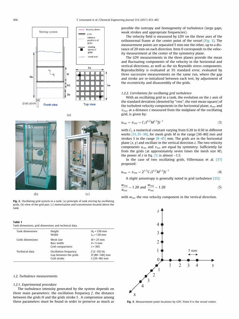
Fig. 2. Oscillating grid system in a tank: (a) principle of tank stirring by oscillatinggrids, (b) view of the grid pair, (c) motorization and transmission located above thetank.

Table 1Tank dimensions, grid dimensions and technical data.

Tank dimensions Height H0 = 330 mmWidth L0 = 130 mm

Grids dimensions Mesh size M = 25 mmBars width d = 5 mmGrid compactness d = 36%

Technical data Oscillation frequency f [2–10] HzGap between the grids H [80–140] mmGrid stroke S [20–40] mm

Fig. 3. Measurement point locations by LDV. Point 0 is the vessel center.

456 T. Lemenand et al. / Chemical Engineering Journal 314 (2017) 453–465

1.2. Turbulence measurements

1.2.1. Experimental procedureThe turbulence intensity generated by the system depends on

three main parameters: the oscillation frequency f , the distancebetween the grids H and the grids stroke S . A compromise amongthese parameters must be found in order to preserve as much as

possible the isotropy and homogeneity of turbulence (large gaps,weak strokes and appropriate frequencies).

The velocity field is measured by LDV on the three axes of theorthonormal frame at the center point of the vessel (Fig. 3). Themeasurement points are separated 5 mm one the other, up to a dis-tance of 20 mm on each direction. Item 0 corresponds to the veloc-ity measurement at the center of the symmetry plane.

The LDV measurements in the three planes provide the meanand fluctuating components of the velocity in the horizontal andvertical directions, as well as the six Reynolds stress components.Reproducibility is evaluated at 5% standard error, evaluated bythree successive measurements on the same run, where the gapand stroke are re-initialized between each test, by adjustment ofthe eccentricity and disassembly of the grids.

1.2.2. Correlations for oscillating grid turbulenceWith an oscillating grid in a tank, the evolution on the z axis of

the standard deviation (denoted by ‘‘rms”, the root mean square) ofthe turbulent velocity components in the horizontal plane, urms andvrms, at a distance z measured from the midplane of the oscillatinggrid, is given by:

urms ¼ v rms ¼ C1S3=2M1=2fz�1 ð3Þ

with C1 a numerical constant varying from 0.20 to 0.50 in differentworks [31,35–38], for mesh grids M in the range [30–80] mm andstrokes S in the range [8–45] mm. The grids are in the horizontalplane (x, y) and oscillate in the vertical direction z. The two velocitycomponents urms and v rms are equal by symmetry. Sufficiently farfrom the grids (at approximately seven times the mesh size M),the power of z in Eq. (3) is almost –1.5.

In the case of two oscillating grids, Villermaux et al. [37]proposed:

urms ¼ v rms ¼ 21=3C1S3=2M1=2fz�1 ð4Þ

A slight anisotropy is generally noted in grid turbulence [35]:

wrms

urms� 1:20 and

wrms

v rms� 1:20 ð5Þ

with wrms the rms velocity component in the vertical direction.

T. Lemenand et al. / Chemical Engineering Journal 314 (2017) 453–465 457

1.3. Homogeneity and isotropy in the vessel core

1.3.1. LDV measurements in the vessel center and vicinityTemporal signals of the longitudinal velocity fluctuations are

recorded using LDV at the locations marked in Fig. 3. The spectraare presented in pre-multiplied format, i.e. based on the powerspectral density multiplied by the frequency plotted versus fre-quency on a semi-log scale. The turbulent kinetic energy (TKE) kis hence visualized by the area below the curve [39,40]. As anexample, the pre-multiplied spectra of velocity fluctuations for afrequency of 6 Hz, a gap of 120 mm, and a stroke of 40 mm, forthe two velocity components u and w on the x and z coordinatesare shown in Fig. 4 (the horizontal velocity component v is notshown because it is identical to u for symmetry reasons).

A satisfactory homogeneity (spatial invariance) is observed onthe (x, y) plane since (as shown in Fig. 4(a) and Fig. 4(c)) all profilesmerge to a single curve. An energy peak appears at grid oscillationfrequency 6 Hz, which corresponds to the flow structures releasedby the grid; however, this remains a weak contribution to the glo-bal kinetic energy. The homogeneity on the vertical axis can beobserved in Fig. 4(b) and Fig. 4(d) and is valid up to z ¼ 10 mm.This implies that a zone of 10 mm around the central point 0 canbe considered homogeneous.

The root mean square values of the turbulent velocity compo-nents are in fair agreement with the theoretical model in Eq. (4)

Fig. 4. Pre-multiplied energy spectra for horizontal velocity component u: (a) along x, (bH = 120 mm, S = 40 mm.

as shown in Fig. 5; the deviation between theory and measure-ments is less than 6%. In this case, the constant C1 ¼ 0:233.

1.3.2. IsotropyThe ratio of fluctuating velocity components for the vertical and

horizontal directions wrms=urms shown in Fig. 6 characterizes theisotropy provided by the active grid system at the center of thevessel, and lies at around 1.30 ± 6%, of the same order found inthe literature (Eq. (5)). The isotropy is better for the smaller strokes(S ¼ 20 mm) and the larger distances between the grids(H ¼ 100 and 120 mm), but no general law seems to emerge. Forexample, the isotropy is excellent (wrms=urms � 1:00) for a fre-quency f ¼ 4 Hz, a height of H ¼ 100 mm, and a strokeS ¼ 20 mm, and also for f ¼ 8 Hz, H ¼ 120 mm, S ¼ 20 mm.

1.3.3. HomogeneityThe main advantage of using two active grids is that the central

point is a zero-gradient location for symmetry reasons [37]. Theissue is the robustness of this feature in the vicinity of the point0; that is, to ensure a reliable 0-dimensional situation regardlessof any inaccuracy in the central location. The horizontal and verti-cal fluctuating velocities u and w appear to be quite constant in thehorizontal plane ðx; yÞ, with a measurement error of 6%. Fig. 7 and

Fig. 8 show the dimensionless group k1=2=fS calculated based on the

) along z, and for vertical velocity component w: (c) along x, (d) along z, for f = 6 Hz,

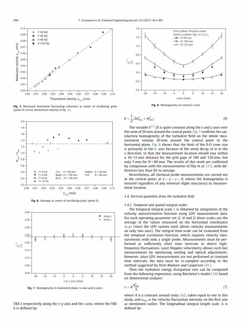
Fig. 5. Measured horizontal fluctuating velocities at center of oscillating grids(point 0) versus theoretical velocity of Eq. (4).

Fig. 6. Isotropy at center of oscillating grids (point 0).

Fig. 7. Homogeneity in horizontal plane (x-axis and y-axis).

Fig. 8. Homogeneity on vertical z-axis.

458 T. Lemenand et al. / Chemical Engineering Journal 314 (2017) 453–465

TKE k respectively along the x /y axis and the z axis, where the TKEk is defined by:

k ¼ 12ð2u2

rms þw2rmsÞ ð6Þ

The variable k1=2=fS is quite constant along the x and y axes overthe zone of 20 mm around the central point. Fig. 7 confirms the sat-isfactory homogeneity of the turbulent field on the whole mea-surement volume 20 mm around the central point in thehorizontal plane. Fig. 8 shows that the limit of the 0-D zone sizeis primarily in the z -axis because of the steep decay of w in thez direction, so that the measurement location should stay withina 10–15 mm distance for the grid gaps of 100 and 120 mm, butonly 5 mm for H = 80 mm. The results of this work are confirmedby comparison with the measurements of Shy et al. [31], with dif-ferences less than 9% in average.

Nevertheless, all chemical probe measurements are carried outat the central point, at x ¼ y ¼ z ¼ 0, where the homogeneity isensured regardless of any eventual slight inaccuracy in measure-ment location.

1.4. Derived quantities from the turbulent field

1.4.1. Temporal and spatial integral scalesThe temporal integral scale s is obtained by integration of the

velocity autocorrelation function using LDV measurement data.For each operating parameter set (f , H and S) these scales are theaverage of the values measured on the horizontal coordinatesðx; yÞ (since the LDV system used allows velocity measurementson only two axes). The integral time-scale can be evaluated fromthe temporal correlation function, which requires velocity mea-surements with only a single probe. Measurements must be per-formed at sufficiently short time intervals to detect high-frequency fluctuations. Laser Doppler velocimetry allows such fastmeasurements by optimizing seeding and optical adjustments.However, since LDV measurements are not performed at constanttime intervals, the data must be re-sampled according to themethod suggested by Host-Madsen and Caspersen [41].

Then the turbulent energy dissipation rate can be computedfrom the following expression, using Batchelor’s model [10] basedon dimensional analysis:

e ¼ Au3rms

Kð7Þ

where A is a constant around unity [42], taken equal to one in thisstudy, and urms is the velocity fluctuation intensity on the first axisas mentioned earlier. The longitudinal integral length scale K isdefined by:

T. Lemenand et al. / Chemical Engineering Journal 314 (2017) 453–465 459

K ¼Z 1

0

u0ðxÞu0ðxþ rÞu02ðxÞ

dr ð8Þ

Here u0 refers to the instantaneous fluctuating velocity. The spa-tial autocorrelation, which is not accessible by LDV measurement,is deduced from the temporal macro scale, determined by the tem-poral autocorrelation:

s ¼Z 1

0

u0ðtÞu0ðt þ TÞu02ðtÞ dT ð9Þ

with the Taylor assumption of frozen turbulence:

K ¼ urmss ð10ÞValues of K reported in Fig. 9 are consistent with the orders of

magnitude quoted in similar flow [31]. Values of K are representedin comparison with the Taylor micro-scale k versus the Reynoldsnumber based on the Taylor scale Rek, which is commonly usedto characterize grid turbulence. The ratio k=urms characterizes thetime-scale of the small eddies. For homogenous and isotropicturbulence:

k ¼ 30vu2rms

e

� �1=2

ð11Þ

and

Rek ¼ urmskv ð12Þ

In the range of parameters of Reynolds number Rek [15–80], theintegral scale K increases with Rek while the Taylor micro-scale kdecreases, indicating the extension of the inertial range.

1.4.2. TKE dissipation rateTwo models to estimate the TKE dissipation rate e, valid for an

oscillating grid, are used. The first, due to Kit et al. [36], is sug-gested for an oscillating grid at frequencies 2–4 Hz, a mesh sizeof 80 mm, and a stroke of 32 mm, in a vessel of 450 mm. It shouldbe noted that the fluctuating velocity used in this paper is the ver-tical velocity component wrms:

e ¼ 0:75w3

rms

Kð13Þ

The second model was proposed by Bache et al. [43] with anempirical correlation based on measurement of the power injectedin the fluid by the grid, in the case of a fine mesh (10 mm) and highfrequencies (15–40 Hz):

Fig. 9. Spatial integral scale K and Taylor micro-scale k.

e ¼ 2:40u2rms

sð14Þ

The TKE dissipation rates e are plotted in Fig. 10 as a function ofthe TKE k . Values obtained by the two above methods are alsoplotted on the same figure; they are in relatively good agreementwith the order of magnitude of the present measurements, partic-ularly for high TKE levels. The TKE dissipation rates measured inthis study appear to be underestimated compared to the literature,by a factor of 1.50 compared to the results of Kit et al. [36] and 1.94compared to those of Bache et al. [43]. This may be due to the valueof the constant A in Eq. (7) (taken equal to 1 in this study), which isnot an absolute constant: the constant can be greater than one,especially when turbulence is relatively weak [42]; for instance,Mohand Kaci et al. [44,45] reported A = 1.85 in a tube equippedwith vortex generators at the wall.

2. Chemical probe measurements

2.1. Principle of the chemical probe - iodure/iodate system

An increasing literature proposes the use of chemical reactionsfor local measurement of micro-mixing in a turbulent flow [46–48]. The chemical probe is generally based on the measurementof the S species of the secondary reaction in a parallel-competitive system:

Aþ B ! R ð15Þ

C þ B ! S ð16ÞFor this, the reaction (15) is fast compared to the reaction (16),

and the characteristic time tr2 of reaction (16) must be of the sameorder of magnitude as that of the micro-mixing tm wewant to mea-sure (the ‘‘local” mixing must be limiting). Reagents A and C arepreviously diluted in the main flow in stoichiometric excess. Asmall quantity of reagent B (in stoichiometric deficit) is injectedlocally into the flow. The reaction rate is hence governed by themicro-mixing, as shown in Fig. 11. The composition of the chemi-cals at the exit determines the segregation index XS, which is theratio between the quantity of B transformed into S and the initialquantity of B.

Previous work of Fournier et al. [19] and Guichardon and Falk[20] have detailed an experimental procedure for using the

Fig. 10. TKE dissipation rate versus TKE in grid turbulence measured at point 0 –comparison of present results with those of Bache et al. [43] and Kit et al. [36].

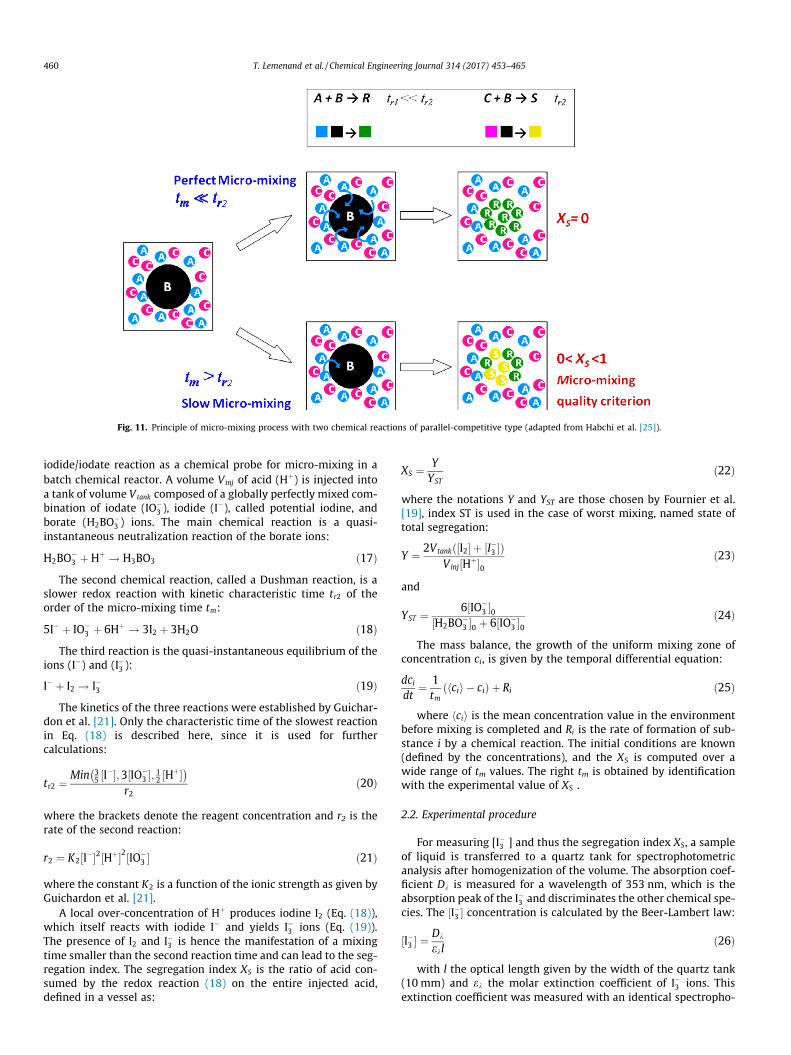
Fig. 11. Principle of micro-mixing process with two chemical reactions of parallel-competitive type (adapted from Habchi et al. [25]).

460 T. Lemenand et al. / Chemical Engineering Journal 314 (2017) 453–465

iodide/iodate reaction as a chemical probe for micro-mixing in abatch chemical reactor. A volume Vinj of acid (Hþ) is injected intoa tank of volume Vtank composed of a globally perfectly mixed com-bination of iodate (IO�

3 ), iodide (I�), called potential iodine, andborate (H2BO

�3 ) ions. The main chemical reaction is a quasi-

instantaneous neutralization reaction of the borate ions:

H2BO�3 þHþ ! H3BO3 ð17Þ

The second chemical reaction, called a Dushman reaction, is aslower redox reaction with kinetic characteristic time tr2 of theorder of the micro-mixing time tm:

5I� þ IO�3 þ 6Hþ ! 3I2 þ 3H2O ð18Þ

The third reaction is the quasi-instantaneous equilibrium of theions (I�) and (I�3 ):

I� þ I2 ! I�3 ð19ÞThe kinetics of the three reactions were established by Guichar-

don et al. [21]. Only the characteristic time of the slowest reactionin Eq. (18) is described here, since it is used for furthercalculations:

tr2 ¼ Min 35 ½I��;3½IO�

3 �; 12 ½Hþ�� �r2

ð20Þ

where the brackets denote the reagent concentration and r2 is therate of the second reaction:

r2 ¼ K2½I��2½Hþ�2½IO�3 � ð21Þ

where the constant K2 is a function of the ionic strength as given byGuichardon et al. [21].

A local over-concentration of Hþ produces iodine I2 (Eq. (18)),which itself reacts with iodide I� and yields I�3 ions (Eq. (19)).The presence of I2 and I�3 is hence the manifestation of a mixingtime smaller than the second reaction time and can lead to the seg-regation index. The segregation index XS is the ratio of acid con-sumed by the redox reaction (18) on the entire injected acid,defined in a vessel as:

XS ¼ YYST

ð22Þ

where the notations Y and YST are those chosen by Fournier et al.[19], index ST is used in the case of worst mixing, named state oftotal segregation:

Y ¼ 2Vtankð½I2� þ ½I�3 �ÞVinj½Hþ�0

ð23Þ

and

YST ¼ 6½IO�3 �0

½H2BO�3 �0 þ 6½IO�

3 �0ð24Þ

The mass balance, the growth of the uniform mixing zone ofconcentration ci, is given by the temporal differential equation:

dcidt

¼ 1tm

ðhcii � ciÞ þ Ri ð25Þ

where hcii is the mean concentration value in the environmentbefore mixing is completed and Ri is the rate of formation of sub-stance i by a chemical reaction. The initial conditions are known(defined by the concentrations), and the XS is computed over awide range of tm values. The right tm is obtained by identificationwith the experimental value of XS .

2.2. Experimental procedure

For measuring [I�3 ] and thus the segregation index XS, a sampleof liquid is transferred to a quartz tank for spectrophotometricanalysis after homogenization of the volume. The absorption coef-ficient Dk is measured for a wavelength of 353 nm, which is theabsorption peak of the I�3 and discriminates the other chemical spe-cies. The ½I�3 � concentration is calculated by the Beer-Lambert law:

½I�3 � ¼Dk

eklð26Þ

with l the optical length given by the width of the quartz tank(10 mm) and ek the molar extinction coefficient of I�3 ions. Thisextinction coefficient was measured with an identical spectropho-

Fig. 12. Segregation index XS according to Reynolds number based on Taylor micro-scale Rek .

T. Lemenand et al. / Chemical Engineering Journal 314 (2017) 453–465 461

tometer at 2606 m2 mol�1 by Ferrouillat et al. [48] and 2590 m2 -mol�1 by Fournier et al. [19]. By comparison, the extinction coeffi-cient of iodine at 353 nm is equal to 2 m2 mol�1 [49].

Once the adjustments are made, the experiment starts by set-ting the electric motor at a given oscillation frequency. After wait-ing several minutes to reach steady state, the sulphuric acid isinjected. For experimental reliability, the injection time must belong compared with the macro-mixing and meso-mixing time,and so that the injection flow is ensured not to perturb the localturbulence, by assessing the independence of XS with respect tothe flow-rate. Visual monitoring checks for the absence of struc-tures resulting from jet turbulence. The injected volume must beas small as possible to ensure local measurements; the volumesare respectively 5 mL and 10 mL for Run 5 and Run 6 during600 s, which provides smaller flow-rates than Fournier et al. [19],around 1 mL/min. The run identifications are those used by Four-nier et al. [19], details of which are reported in Table 2. Whenthe injection is completed, the agitation frequency is then regu-lated at its maximum for a duration of one minute in order tohomogenize the whole tank, and then the electric motor isstopped. A sample can now be taken by a 50 mL syringe foranalysis.

For each operating condition (frequency, height and stroke ofgrid), three successive injections of acid allow three measurementsof XS for the same initial solution. The first measurement of XS isdone knowing the initial concentrations. For the second injection,knowing the acid quantity that participated in the acid-base reac-tion and with the redox reaction during the first injection, all con-centrations are re-initialized to calculate new XS . This process isrepeated until the absorption measurement of I�3 becomes impos-sible in the spectrophotometer.

A matter balance from the stoichiometric Eqs. (17)–(19) is thenused to calculate XS . Finally, XS is determined with a relative pre-cision of 6%.

2.3. Segregation index measurements

Three series of measurements of the segregation index XS arecarried out for the different reagents concentrations shown inTable 2: first, a strong iodine concentration coupled with a weakacid concentration (Runs 5 and 6), and second, a weak iodine con-centration coupled with a strong acid concentration (Run 2). Thetwo first runs are the least economical solution because of the lar-ger quantity of iodized reagents used.

Experimental measurements of the segregation index XS

obtained in grid turbulence in this study (homogeneous case) aresummarized in Fig. 12. Following the acid concentration, the levelof XS is different for the same hydrodynamic conditions and thus isnot an intrinsic measurement of micro-mixing. Acid concentration½Hþ� ¼ 0:08 mol=L gives a segregation index greater than thoseobtained at ½Hþ� ¼ 0:04 mol=L, as confirmed by the results of Four-nier et al. (1996): the measured value of XS is directly influenced bythe acid concentration.

Fig. 12 also highlights a linear decrease of XS with the TaylorReynolds number Rek as observed in Fournier et al. [19]. The slopesof the segregation index as a function of Rek are almost the same

Table 2Concentrations used for the chemical probe.

Run* ½Hþ�0 (mol/L)

Fournier et al. [19] Run 5 0.08Run 6 0.04

Guichardon et al. [20] Run 2 1.00

* The runs identification used by Fournier et al. [19] and Guichardon et al. [20] are pr

for low acid concentrations ½Hþ� ¼ 0:08 mol=L and½Hþ� ¼ 0:04 mol=L. For these acid concentrations, potential iodineis the same, ½I2�potential ¼ 0:07 mol=L. On the other hand, for the

results obtained with ½Hþ� ¼ 1:00 mol=L, the slope is half as large:in this case, potential iodine is ten times lower,½I2�potential ¼ 0:007 mol=L. Thus the greater the iodine concentration,the greater the slope, and XS measurement is then more sensitiveto small turbulence variations.

3. Micro-mixing time

In order to quantify the micro-mixing independently of thechemical reaction, it must be modeled in a simple framework thatcan relate a measured segregation rate XS to a micro-mixing timetm . This time tm must depend only on the turbulence occurringat the position where the reactant B is injected. Interest is thusgrowing in modeling the micro-mixing to establish the linkbetween the progress of the chemical reaction and the micro-mixing process. These micro-mixing models quantify the share ofthe reagents perfectly mixed on a molecular scale – and thus avail-able for the reaction – by fitting a micro-mixing time associated tothe scalar exchange between a perfectly mixed fluid fraction andthe surrounding fluid in 0�dimensional flows. Here two determin-istic models are described and compared: IEM and EDD models.

3.1. IEM model

The IEM (Interaction Exchange with the Mean) model is a ‘‘two-environment” model developed on the basis of the coalescence re-dispersion model [50], which is a stochastic mixing model. Theauthors globalize the coalescence re-dispersion model to get adeterministic formulation that requires less computer capacity.The IEMmodel was validated for a chemical reaction in a dispersedphase in a reactor and extended to a single-phase flow. The authors

½I2�potential 0 (mol/L) ½H2BO�3 �0 (mol/L)

7 � 10�2 5.66 � 10�2

7 � 10�2 5.66 � 10�2

7 � 10�3 9.09 � 10�2

eserved for more clearness.

462 T. Lemenand et al. / Chemical Engineering Journal 314 (2017) 453–465

underline the difficulty of studying the micro-mixing indepen-dently from macro-mixing, and thus this model can include bothmacro- and micro-mixing, according to the objectives.

In this model it is assumed that at a given instant one chemicalspecies is concentrated in the b environment and mass transfertakes place with the chemical species in the a environment(Fig. 13). The respective volumes of a and b are constant over time.The intensity of the exchange is scaled by an exchange coefficientkm estimated from a characteristic frequency for isotropic turbu-lent flows [51] corresponding to the characteristic time of the tur-bulent cascade:

km ¼ 1tm IEM

¼ 1C1

ek

ð27Þ

where C1 is a constant of order 0.5 and tm IEM is the micro-mixingtime in the IEM model:

tm IEM ¼ C1ke

ð28Þ

The micro-mixing time tm IEM was experimentally confirmed inchemical reactors by several authors [52,53], and the IEM modelwas coupled with information from residence time distribution.This time-scale is generally used with two assumptions. First, thecascade of turbulent kinetic energy produced at large scales is inequilibrium, with its dissipation occurring around the Kolmogorovscale. Second, the cascade time (Corssin time scale) defined by

tt ¼ ke

ð29Þ

is proportional to the scalar variance dissipation time th:

th ¼ Rtt ð30Þwith R a constant. Several authors have shown that R in the

range 0.6–3.1 is not a universal constant and depends on the scalarscales [54]. The concentration evolution for the a and b environ-ments is given by:

dca or b

dt¼ kmðhci � ca or bÞ ð31Þ

where ca or b is the scalar concentration in the a or b environ-ment and hci the mean concentration of the scalar in the wholezone, given by:

hci ¼ Vaca þ VbcbVa þ Vb

ð32Þ

with Va the volume of a and Vb the volume of b . The advantageof the IEM model lies in its simplicity. Its principal disadvantage isthe lack of physical links with the mixing mechanism at smallscales. Moreover, its micro-mixing time is not clearly (experimen-tally) defined in relation to the turbulence properties.

Fig. 13. IEM model.

3.2. EDD model

The EDD (Engulfment, Deformation and Diffusion) model is a‘‘two-environment” model: blobs of one fluid environment erodeto the benefit of the second environment by fluid breakage anddeformation; the final mixing occurs by molecular diffusion.Bałdyga and Bourne [4] showed that in the first step, the blobsbreak up by turbulent cascade in the inertial zone and aredeformed in the second step by fine-scale turbulence; the thirdstep is laminar stretching at the Kolmogorov scale and the fourthis the engulfment process. The restrictive step for molecular mix-ing is this engulfment process: the engulfment mechanism reducesthe non-homogeneity scale by incorporation of the surroundingfluid A in the volume B by the most hydrodynamically active vor-tices (Fig. 14). These vortices produce a stretched and folded struc-ture of A and B that reduces the scale of A and B (striationthicknesses) until the Batchelor scale is reached; this permits themolecular diffusion mechanism to come to action at the interfacesbetween A and B.

During engulfment, the B environment is assumed to be wellmixed at all scales, even after the incorporation of a certain volumeof A. The growth of the volume VðtÞ of this perfectly mixed envi-ronment is given by an equation involving the characteristicgrowth time sw:

VðtÞ ¼ Vð0Þ2t=sw ð33Þidentified by

VðtÞ ¼ Vð0ÞeEt ð34Þto give E, the engulfment parameter. The micro-mixing time

tmEDD is then given by:

tmEDD ¼ 1E

ð35Þ

The evolution of the quantity n of scalar in the volume VðtÞ isgiven by q, the rate of incorporation:

dndt

¼ c0q ¼ dðcVÞdt

ð36Þ

where c0 is the concentration of the scalar outside the volumeVðtÞ and c the concentration inside VðtÞ . Defining a first orderlaw for the volume increase:

q ¼ dVdt

¼ EV ð37Þ

These two Eqs. (36) and (37) lead to the kinetic equation for thismicro-mixing model:

dcdt

¼ Eðc0 � cÞ ð38Þ

In the EDDmodel, the external concentration c0 is constant overtime but the reference volume grows. Thus the mean concentra-tion is given by:

hci ¼ VðtÞc þ ½Vt � VðtÞ�c0Vt

ð39Þ

where Vt is the total volume.

3.3. Micro-mixing time results

Experimental micro-mixing times are computed with a numer-ical model, by an ‘‘inverse method” that is applied to yield thesame segregation index XS as the experimental data. The numericalresolution is carried out by integration over time of the set of equa-tions (31) for IEM and (38) for EDD, for each chemical species of theiodide/iodate system.

Fig. 14. Schematic engulfment process of the engulfment model.

Fig. 16. Experimental micro-mixing time tmEDD using EDD model versus thedissipation rate e.

T. Lemenand et al. / Chemical Engineering Journal 314 (2017) 453–465 463

Fig. 15 shows the computed results of the IEM micro-mixingtime tm IEM plotted in log-log scale versus the turbulent dissipationrate e obtained by LDA. It is first observed that this model is highlysensitive to the acid concentration. On the one hand, no solutioncan be attained with ½Hþ� ¼ 1:00 mol=L. On the other, for½Hþ� ¼ 0:08 mol=L one notes that tm IEM exceeds 1 s for a turbulentenergy dissipation rate e in the range studied [5 � 10�4–10�1]m2 s�3, much more than Baldyga’s model predicts, and moreoverthe trend is not consistent with the �1=2 law power of e by thatsame model.

tm IEM ¼ CIEMte

� �1=2ð40Þ

Unfortunately, the value of the constant CIEM ¼ 32:4 is muchhigher than 17.24 given by Bałdyga and Bourne [4] in Eq. (1); evenin this case the error in the micro-mixing time is about 88%.

Fig. 16 shows the results of EDD micro-mixing time tmEDD in asimilar representation. It is first observed that the micro-mixingtimes appear rather independent of the operating conditions, evenwith an order-of-magnitude difference in the acid concentrations.In particular, the results are consistent for the more intense turbu-lence, that is for e > 10�2 m2 s�3 (i.e. Reynolds number Rek > 35).Moreover, the micro-mixing time tmEDD seems to be well scaledby the Kolmogorov time-scale with the �1/2 log-slope and has val-ues much closer to Baldyga’s model. By fitting the experimentalresults with the expression

tmEDD ¼ CEDDte

� �1=2ð41Þ

it is found that CEDD ¼ 12:7 for the whole set of experiments,which is in quite better agreement with the value of 17.24 reportedin Eq. (1). In greater detail, the results for the runs½Hþ� ¼ 0:04 mol=L and 0.08 mol/L are generally more satisfactoryfor the whole range of e . For ½Hþ� ¼ 1:00 mol=L, the results for

Fig. 15. Experimental micro-mixing time tmIEM using IEM model versus thedissipation rate e.

tmEDD are actually consistent with e > 10�2 m2 s�3 (i.e. Rek > 35),but for e < 10�2 m2 s�3 (i.e. Rek < 35) tmEDD seems to move awayfrom the prediction. For low turbulence levels, some limitationsin accuracy appear for the method, suggesting that the choice ofoperating concentration is important. By eliminating this fractionof the experiments, i.e. considering only the results for e > 10�2

m2s�3, the constant of Eq. (41) is CEDD ¼ 15:9 (bold line in Fig. 16).

4. Discussion

The IEM model is very sensitive to the change in species con-centration. For the higher acid concentration, i.e.½Hþ� ¼ 1:00 mol=L, the IEM model failed to reproduce the level ofXS . In this case, the simulated XS is below the experimental value,implying that the IEM model underestimates iodine production.Various features may explain this result.

Consider Eq. (42) representing the molar flux of acid that goesfrom a b environment where acid is predominant to an a environ-ment where borate ions predominate:

Acid fluxðbÞ!ðaÞ ¼Dttm

½Hþ� VtankVinj

Vtank þ Vinjð42Þ

This flux increases with acid concentration, and the acid trans-ferred in the a environment fully reacts with the borate ions. Thusthe higher this flux, the less can acid reacts with iodide and iodateto create iodine. For high acid concentration, the IEM model favorsthe reaction (15). Moreover, the volumes of a and b were chosen inorder to represent the acid volume and tank volume. Thus, theinteraction between the fraction of fluid where the chemical reac-tions occur and the fresh fluid is neglected, so that the IEM modelfails to describe the mixing process properly. For these reasons,this model cannot be used for local simulation of micro-mixingand must be modified to better account for the local aspect ofthe injection and limit its sensitivity to the concentrations.

464 T. Lemenand et al. / Chemical Engineering Journal 314 (2017) 453–465

A contrario, the construction of the EDD model can explain itsrobustness. Actually, EDD model ‘‘considers” a medium of acid inwhich the micro-mixing mechanism incorporates a fraction ofthe reagents of the surrounding medium, the buffer solution andpotential iodine. The acid is always dominating in a perfectly agi-tated medium, and thus the micro-mixing, which controls thequantity of incorporated matter, readily determines the quantityof iodine formed. It thus seems logical that the micro-mixing phe-nomenon primarily determines the segregation index XS .

This benchmarking shows that EDD model is more adapted tochemical probe analysis, unless the choice of the concentrationsis an issue. Moreover, this model consumes less machine timeand is simpler to implement since it requires few parameters.

5. Conclusions

The chemical probe is a series of reactions whose kinetics is ofthe order of the micro-mixing rate, which hence becomes indi-rectly observable. The general configuration in which the chemicalprobe method was used, like stirred vessels or static mixers, do notlet us assess the validity of micro-mixing models since the condi-tions are far from HIT turbulence, which is the grounding assump-tion of these models. This induces bias in the results because ofadvection and turbulent field gradients.

To the best of our knowledge, no earlier work reports on micro-mixing measurements in a turbulence approaching isotropy andhomogeneity with no mean flow. In the present work, chemicalprobe measurements are carried out in a stirred vessel with a pairof oscillating grids providing a satisfying HIT, for different operat-ing conditions (stroke and frequency) and reagent concentrations.The IEM and EDD micro-mixing models can hence be tested inclose to ideal conditions and their results can be compared withthe theory.

The IEM model appears to be highly sensitive to the acid con-centration and cannot be used with confidence for local measure-ment for intrinsic characterization of micro-mixing, while EDDmodel seems to deal consistently with the chemical probe data.The latter model can be taken as a reference among the determin-istic micro-mixing models in further experiments. Future work willfocus on investigation of the appropriate concentrations and on thedeviation of the chemical probe in non-ideal conditions of the com-plex geometries in real chemical reactors.

Acknowledgements

Authors would like to acknowledge C. Durandal for his implica-tion in the experimental work.

References

[1] A. Ghanem, T. Lemenand, D. Della Valle, H. Peerhossaini, Static mixers:mechanisms, applications, and characterization methods – a review, Chem.Eng. Res. Des. 92 (2014) 205–228.

[2] C. Habchi, T. Lemenand, D. Della Valle, M. Khaled, A. Elmarakbi, H.Peerhossaini, Mixing assessment by chemical probe, J. Ind. Eng. Chem. 20(2014) 1411–1420.

[3] H.J. Yang, G.W. Chu, Y. Xiang, J.F. Chen, Characterization of micromixingefficiency in rotating packed beds by chemical methods, Chem. Eng. J. 121(2006) 147–152.

[4] J. Baldyga, J.R. Bourne, Turbulent Mixing and Chemical Reactions, Wiley, 1999.[5] S.W. Jones, O.M. Thomas, H. Aref, Chaotic advection by laminar flow in a

twisted pipe, J. Fluid Mech. 29 (1989) 335–357.[6] C. Habchi, S. Ouarets, T. Lemenand, D. Della Valle, J. Bellettre, H. Peerhossaini,

Influence of viscosity ratio on droplets formation in a chaotic advection flow,Int. J. Chem. React. Eng. 7 (2009).

[7] F.J. Muzzio, C. Meneveau, P.D. Swanson, Scaling and multifractal properties ofmixing in chaotic flows, Phys. Fluids A Fluid (1992) 1439–1456.

[8] R.O. Fox, Computational Models for Turbulent Reacting Flows, CambridgeUniversity Press, 2003.

[9] J. Baldyga, R. Pohorecki, Turbulent micromixing in chemical reactors – areview, Chem. Eng. J. 58 (1995) 183–195.

[10] G.K. Batchelor, The Theory of Homogeneous Turbulence, Cambridge UniversityPress, 1953.

[11] J. Baldyga, W. Podgórska, R. Pohorecki, Mixing-precipitation model withapplication to double feed semibatch precipitation, Chem. Eng. Sci. 50 (1995)1281–1300.

[12] L. Falk, E. Schaer, A PDF modelling of precipitation reactors, Chem. Eng. Sci. 56(2001) 2445–2457.

[13] R. Pohorecki, J. Baldyga, The effects of micromixing and the manner of reactorfeeding on precipitation in stirred tank reactors, Chem. Eng. Sci. 43 (1988)1949–1954.

[14] G. Tosun, A mathematical model of mixing and polymerization in a semibatchstirred-tank reactor, AIChE J. 38 (1992) 425–437.

[15] J. Aubin, M. Ferrando, V. Jiricny, Current methods for characterising mixing andflow in microchannels, Chem. Eng. Sci. 65 (2010) 2065–2093.

[16] N. Kockmann, T. Kiefer, M. Engler, P. Woias, Silicon microstructures for highthroughput mixing devices, Microfluid. Nanofluid. 2 (2006) 327–335.

[17] V. Hessel, S. Hardt, H. Löwe, F. Schönfeld, Laminar mixing in differentinterdigital micromixers: I. Experimental characterization, AIChE J. 49 (2003)566–577.

[18] J. Villermaux (Ed.), Génie de la réaction chimique: conception etfonctionnement des réacteurs, Technique et Documentation, Lavoisier, Paris,1993.

[19] M.-C. Fournier, L. Falk, J. Villermaux, A new parallel competing reaction systemfor assessing micromixing efficiency—experimental approach, Chem. Eng. Sci.51 (1996) 5053–5064.

[20] P. Guichardon, L. Falk, Characterisation of micromixing efficiency by the iodide- iodate reaction system. Part I : experimental procedure, Chem. Eng. Sci. 55(2000) 4233–4243.

[21] P. Guichardon, L. Falk, J. Villermaux, Characterization of micromixingefficiency by the iodide-iodate reaction system. Part II: kinetic study, Chem.Eng. Sci. 55 (2000) 4245–4253.

[22] J.R. Bourne, M. Lips, Micromixing in grid-generated turbulence: theoreticalanalysis and experimental study, Chem. Eng. J. 47 (1991) 155–162.

[23] M. Assirelli, W. Bujalski, A. Eaglesham, A.W. Nienow, Study of micromixing in astirred tank using a rushton turbine, Chem. Eng. Res. Des. 80 (2002) 855–863.

[24] S. Ferrouillat, P. Tochon, C. Garnier, H. Peerhossaini, Intensification of heat-transfer and mixing in multifunctional heat exchangers by artificiallygenerated streamwise vorticity, Appl. Therm. Eng. 26 (2006) 1820–1829.

[25] C. Habchi, D. Della Valle, T. Lemenand, Z. Anxionnaz, P. Tochon, M. Cabassud,et al., A new adaptive procedure for using chemical probes to characterizemixing, Chem. Eng. Sci. 66 (2011) 3540–3550.

[26] J. Baldyga, J.R. Bourne, Simplification of micromixing calculations. I. Derivationand application of new model, Chem. Eng. J. 42 (1989) 83–92.

[27] J. Baldyga, J.R. Bourne, Comparison of the engulfment and the interaction-by-exchange- with-the-mean micromixing models, Chem. Eng. J. 45 (1990) 25–31.

[28] J. Baldyga, A. Rozen, F. Mostert, A model of laminar micromixing withapplication to parallel chemical reactions, Chem. Eng. J. 69 (1998) 7–20.

[29] C. Durandal, T. Lemenand, D. Della Valle, H. Peerhossaini, A chemical probe forcharacterizing turbulent micromixing, in: ASME Fluids Eng. Div. SummerMeet. Symp. Macro- Micromixing Single Phase Fluids, ASME, Miami, 2006, pp.1091–1099.

[30] S.B. Pope, Turbulent Flows, Cambridge University Press, 2000.[31] S.S. Shy, C.Y. Tang, S.Y. Fann, A nearly isotropic turbulence generated by a pair

of vibrating grids, Exp. Therm. Fluid Sci. 14 (1997) 251–262.[32] K. Abou Hweij, F. Azizi, Hydrodynamics and residence time distribution of

liquid flow in tubular reactors equipped with screen-type static mixers, Chem.Eng. J. 279 (2015) 948–963.

[33] Q. Zhou, N.S. Cheng, Experimental investigation of single particle settling inturbulence generated by oscillating grid, Chem. Eng. J. 149 (2009)289–300.

[34] H.J.S. Fernando, I.P.D. De Silva, Note on secondary flows in oscillating-grid,mixing-box experiments, Phys. Fluids A Fluid Dyn. 5 (1993) 1849.

[35] I.P.D. De Silva, H.J.S. Fernando, Oscillating grids as a source of nearly isotropicturbulence, Phys. Fluids 6 (1994) 2455.

[36] E.L.G. Kit, E.J. Strang, H.J.S. Fernando, Measurement of turbulence near shear-free density interfaces, J. Fluid Mech. 334 (1997) 293–314.

[37] E. Villermaux, B. Sixou, Y. Gagne, Intense vortical structures in grid-generatedturbulence, Phys. Fluids 7 (1995) 2008.

[38] Y. Zellouf, P. Dupont, H. Peerhossaini, Heat and mass fluxes across densityinterfaces in a grid-generated turbulence, Int. J. Heat Mass Transf. 48 (2005)3722–3735.

[39] K.C. Kim, R.J. Adrian, Very large-scale motion in the outer layer, Phys. Fluids 11(1999) 417.

[40] T. Lemenand, P. Dupont, D. Della Valle, H. Peerhossaini, Turbulent mixing oftwo immiscible fluids, J. Fluids Eng. 127 (2005) 1132.

[41] A. Host-Madsen, C. Caspersen, The limitations in high frequency turbulencespectrum estimation using the laser Doppler anemometer, in: Seventh Int.Symp. Appl. Laser Tech. to Fluid Mech., Lisbon, 1994.

[42] K.R. Sreenivasan, On the scaling of the turbulence energy dissipation rate,Phys. Fluids 27 (1984) 1048–1051.

[43] D.H. Bache, E. Rasool, Measurement of the rate of energy dissipation around anoscillating grid by an energy balance approach, Chem. Eng. J. Biochem. Eng. J.63 (1996) 105–115.

T. Lemenand et al. / Chemical Engineering Journal 314 (2017) 453–465 465

[44] H. Mohand Kaci, T. Lemenand, D. Della Valle, H. Peerhossaini, Effects ofembedded streamwise vorticity on turbulent mixing, Chem. Eng. Process.Process Intensif. 48 (2009) 1459–1476.

[45] H. Mohand Kaci, C. Habchi, T. Lemenand, D. Della Valle, H. Peerhossaini, Flowstructure and heat transfer induced by embedded vorticity, Int. J. Heat MassTransf. 53 (2010) 3575–3584.

[46] W. Jiao, Y. Liu, G. Qi, A new impinging stream–rotating packed bed reactor forimprovement of micromixing iodide and iodate, Chem. Eng. J. 157 (2010) 168–173.

[47] M. Bertrand, N. Lamarque, O. Lebaigue, E. Plasari, F. Ducros, Micromixingcharacterisation in rapid mixing devices by chemical methods and LESmodelling, Chem. Eng. J. 283 (2016) 462–475.

[48] S. Ferrouillat, P. Tochon, H. Peerhossaini, Micromixing enhancement byturbulence: application to multifunctional heat exchangers, Chem. Eng.Process. Process Intensif. 45 (2006) 633–640.

[49] T.L. Allen, R.M. Keefer, The formation of hypoiodous acid and hydrated iodinecation by the hydrolysis of iodine, J. Am. Chem. Soc. 77 (1955) 2957–2960.

[50] R.L. Curl, Dispersed phase mixing: I. Theory and effects in simple reactors,AIChE J. 9 (1963) 175–181.

[51] S.B. Pope, PDF methods for turbulent reactive flows, Prog. Energy Combust. Sci.11 (1985) 119–192.

[52] X. Guo, Y. Fan, L. Luo, Mixing performance assessment of a multi-channel miniheat exchanger reactor with arborescent distributor and collector, Chem. Eng.J. 227 (2013) 116–127.

[53] M. Kashid, A. Renken, L. Kiwi-Minsker, Mixing efficiency and energyconsumption for five generic microchannel designs, Chem. Eng. J. 167 (2011)436–443.

[54] M. Gonzalez, A. Fall, The approach to self-preservation of scalar fluctuationsdecay in isotropic turbulence, Phys. Fluids 10 (1998) 654.