Embed Size (px)
Citation preview
Micro-Macro-Relations in the Kirk-Coleman-Model
Gero Schwenk
24.05.2004


Abstract
The subject of this work is the analysis of level-transition and emergence prob-lems. Philosophical argument is basically grounded on concepts of object identityand manipulation. It is furthermore extended to criticism of the methodology ofbridge-hypotheses as proposed by methodological individualism in the social sciences. Inorder to provide an actual example, the proposed methodology is implemented: Area ofapplication is the classical Kirk-Coleman-Model, a simulation of interaction behavior ina three-person group. In order to meet the requirements of the proposed methodologyof level-transitory explanation the model is modified and implemented employing thepowerful Bayesian-Network formalism.
The author can be contacted by e-mail: [email protected]

Contents
List of Figures vii
1 Introduction 1
2 Level-Transitory Explanation and Emergence 32.1 Epistemic Account on Object Identity . . . . . . . . . . . . . . . . . . . . . 32.2 Realization of Macroscopic Properties . . . . . . . . . . . . . . . . . . . . . 42.3 Level-Transition . . . . . . . . . . . . . . . . . . . . . . . . . . . . . . . . . 5
2.3.1 Bridge Hypotheses and Violation of Object Identity . . . . . . . . . 52.3.2 Proxy-Descriptions . . . . . . . . . . . . . . . . . . . . . . . . . . . . 6
2.4 Reduction and Manipulation . . . . . . . . . . . . . . . . . . . . . . . . . . 62.4.1 Hypothesis or Definition? . . . . . . . . . . . . . . . . . . . . . . . . 7
2.5 Emergence . . . . . . . . . . . . . . . . . . . . . . . . . . . . . . . . . . . . . 82.6 Remarks on Complexity . . . . . . . . . . . . . . . . . . . . . . . . . . . . . 9
3 Aspects of Modelling 113.1 Model . . . . . . . . . . . . . . . . . . . . . . . . . . . . . . . . . . . . . . . 113.2 Model-Calculus . . . . . . . . . . . . . . . . . . . . . . . . . . . . . . . . . . 113.3 Modelling as a Mindset . . . . . . . . . . . . . . . . . . . . . . . . . . . . . 12
4 A Sketch of Bayesian Networks 134.1 Sketch of the Method . . . . . . . . . . . . . . . . . . . . . . . . . . . . . . 134.2 Definition of Bayesian Networks . . . . . . . . . . . . . . . . . . . . . . . . . 15
4.2.1 Decomposition of Joint Probability Distributions . . . . . . . . . . . 154.2.2 Graphs and Conditional Independence . . . . . . . . . . . . . . . . . 164.2.3 Inference in Bayesian Networks . . . . . . . . . . . . . . . . . . . . . 17
5 Probabilistic System Model 195.1 System . . . . . . . . . . . . . . . . . . . . . . . . . . . . . . . . . . . . . . . 19
5.1.1 Graphical Representation . . . . . . . . . . . . . . . . . . . . . . . . 205.1.2 Unfolding and Transition Representation . . . . . . . . . . . . . . . 205.1.3 Transition Graph . . . . . . . . . . . . . . . . . . . . . . . . . . . . . 215.1.4 Representation in Time: Temporal Graph . . . . . . . . . . . . . . . 22
5.2 Bayesian Network Representation . . . . . . . . . . . . . . . . . . . . . . . . 22
iii
6 Methodological Individualism 256.1 The Micro-Macro-Scheme and Methodological Individualism . . . . . . . . . 256.2 Explicit Application of the Micro-Macro-Scheme . . . . . . . . . . . . . . . 266.3 Macro-States and Initial Conditions . . . . . . . . . . . . . . . . . . . . . . 27
6.3.1 Semantics and Bridge-Hypotheses . . . . . . . . . . . . . . . . . . . 286.4 Deduction of Micro-Macro-Hypotheses . . . . . . . . . . . . . . . . . . . . 29
7 The Kirk-Coleman-Model 317.1 Simmel’s Remark . . . . . . . . . . . . . . . . . . . . . . . . . . . . . . . . . 327.2 The Homans-Hypotheses . . . . . . . . . . . . . . . . . . . . . . . . . . . . . 32
7.2.1 Social Behaviorism . . . . . . . . . . . . . . . . . . . . . . . . . . . . 327.2.2 Mutual Reward and Interaction . . . . . . . . . . . . . . . . . . . . . 337.2.3 Condensed Hypotheses . . . . . . . . . . . . . . . . . . . . . . . . . . 33
7.3 The Kirk-Coleman-Model . . . . . . . . . . . . . . . . . . . . . . . . . . . . 347.4 Various Group-Interaction Models . . . . . . . . . . . . . . . . . . . . . . . 35
8 Modification of the Kirk-Coleman-Model 378.1 Homans-Hypotheses and Expected Utility . . . . . . . . . . . . . . . . . . . 37
8.1.1 Subjective Expected Utility Theory . . . . . . . . . . . . . . . . . . 378.1.2 Adaptation . . . . . . . . . . . . . . . . . . . . . . . . . . . . . . . . 388.1.3 Optimality and Reinforcement Learning . . . . . . . . . . . . . . . . 398.1.4 Optimality and Expected Utility . . . . . . . . . . . . . . . . . . . . 408.1.5 Evaluation of the Theories . . . . . . . . . . . . . . . . . . . . . . . . 40
8.2 Similarity and Attraction . . . . . . . . . . . . . . . . . . . . . . . . . . . . 418.3 Feedback . . . . . . . . . . . . . . . . . . . . . . . . . . . . . . . . . . . . . 41
8.3.1 Social Impact Theory . . . . . . . . . . . . . . . . . . . . . . . . . . 428.4 Agent Level Theory: Action and Social Influence . . . . . . . . . . . . . . . 42
9 Declaration of the Modified Model 459.1 System Representation . . . . . . . . . . . . . . . . . . . . . . . . . . . . . . 459.2 Transition Graph . . . . . . . . . . . . . . . . . . . . . . . . . . . . . . . . . 47
9.2.1 Demonstration of Parentship Subgraphs . . . . . . . . . . . . . . . . 489.3 Functional Dependencies: Conditional Probability Tables . . . . . . . . . . 51
9.3.1 Subjective Expected Utility Theory . . . . . . . . . . . . . . . . . . 519.3.2 Social Impact Theory . . . . . . . . . . . . . . . . . . . . . . . . . . 529.3.3 Auxiliary Assumptions on Trust . . . . . . . . . . . . . . . . . . . . 53
10 Model Sensitivity 5510.1 Employed Soft- and Hardware . . . . . . . . . . . . . . . . . . . . . . . . . . 5510.2 Solving the Model . . . . . . . . . . . . . . . . . . . . . . . . . . . . . . . . 56
10.2.1 Stochastic Sampling . . . . . . . . . . . . . . . . . . . . . . . . . . . 5610.3 Monte-Carlo Parameter Study . . . . . . . . . . . . . . . . . . . . . . . . . . 57
10.3.1 Illustrations of the Monte-Carlo-Runs . . . . . . . . . . . . . . . . . 5810.3.2 Cluster-Analysis of the Monte-Carlo-Runs . . . . . . . . . . . . . . . 58
v
10.4 Interpretation of the Results . . . . . . . . . . . . . . . . . . . . . . . . . . . 6210.4.1 Comparison to the Original Model . . . . . . . . . . . . . . . . . . . 63
11 Level-Transition Instantiated 6511.1 Bridge Hypothesis: Balance Theory Classification . . . . . . . . . . . . . . . 65
11.1.1 Balance Theory . . . . . . . . . . . . . . . . . . . . . . . . . . . . . . 6611.1.2 Assignment of Model-Realizations to P-O-X Triples . . . . . . . . . 67
11.2 Aggregated Results of Lower Level Inference . . . . . . . . . . . . . . . . . . 68
12 Conclusion 7112.1 Summary: Problems and Solutions . . . . . . . . . . . . . . . . . . . . . . . 7112.2 Outlook . . . . . . . . . . . . . . . . . . . . . . . . . . . . . . . . . . . . . . 72
Bibliography 75
Appendix 79
A Online Provision 81
B Complete Monte-Carlo Results 83

vi
List of Figures
5.1 Example Drawing of a Graph . . . . . . . . . . . . . . . . . . . . . . . . . . 21
6.1 The Coleman-Micro-Macro-Scheme . . . . . . . . . . . . . . . . . . . . . . . 25
9.1 Parentship Subgraph of SEU-Template . . . . . . . . . . . . . . . . . . . . . 489.2 Parentship Subgraph of SIT-Template . . . . . . . . . . . . . . . . . . . . . 499.3 Parentship Subgraph of Trust-Template . . . . . . . . . . . . . . . . . . . . 499.4 Complete Transition Graph . . . . . . . . . . . . . . . . . . . . . . . . . . . 50
10.1 Expectation of Monte-Carlo runs of interaction choice Action1 of agent A1
against time. . . . . . . . . . . . . . . . . . . . . . . . . . . . . . . . . . . . 5910.2 Entropy of Monte-Carlo runs of interaction choice Action1 of agent A1
against time. . . . . . . . . . . . . . . . . . . . . . . . . . . . . . . . . . . . 5910.3 Expectation of Monte-Carlo runs of attitude Attitude1 of agent A1 against
time. . . . . . . . . . . . . . . . . . . . . . . . . . . . . . . . . . . . . . . . . 6010.4 Entropy of Monte-Carlo runs of attitude Attitude1 of agent A1 against time. 6010.5 Expectation of Monte-Carlo runs of Trust Trust1−2 of agent A1 against time. 6110.6 Entropy of Monte-Carlo runs of Trust Trust1−2 of agent A1 against time. . 6110.7 K-Means-Clustering of MC-parameter study results: Plot shows mean
silhouette-values for k-cluster solution. . . . . . . . . . . . . . . . . . . . . . 6210.8 K-Means-Clustering of MC-parameter study results: Plot shows gain in R2
for k-cluster solution as compared to (k − 1)-cluster solution. . . . . . . . . 63
11.1 The P-O-X Triple. . . . . . . . . . . . . . . . . . . . . . . . . . . . . . . . . 6611.2 Balanced Triads, (0 ≡ −, 1 ≡ +) . . . . . . . . . . . . . . . . . . . . . . . . 6711.3 Unbalanced Triads, (0 ≡ −, 1 ≡ +) . . . . . . . . . . . . . . . . . . . . . . . 67
B.1 Plot displaying dynamics of expectations and entropies of all variables si-multaneously. . . . . . . . . . . . . . . . . . . . . . . . . . . . . . . . . . . . 83
vii

Chapter 1
Introduction
The question of level-transitory explanation lies on the very core of both individualisticand collectivistic social science.
The possibility of individualistic sociology depends on a solution to this question,and this question is commonly answered by the famous “Micro-Macro-Scheme,” whichgoes back to McCLELLAND [36] and which is usually attributed to COLEMAN [12].The core concept is to explain collective behavior from individual actions, to name thelevels considered. The same question of level-transition is answered in a different wayby collectivistic sociology: It is taken for granted that properties of collectives cannotbe explained across levels, because of an irreducible process of “emergence”. A classicalpresentation of the positions is given by ALEXANDER et al. [1].
The continuing actuality of the question is reflected by recent works which discussthe issues of reduction and emergence with reference to new theoretical developmentsfrom the field of Philosophy of Mind, compare for example HEINTZ [20] and SAWYER[51] [52].
Both level-transitory explanation and emergence are possible, and the intention ofthis work is to provide a coherent philosophical treatment of the problem which is basedon new epistemological insights. Additionally, a further aim is to show an abstract butactual implementation of level-transitory explanation.
We will see that the answers to the philosophical question of emergence are not soeasily obtained as proposed by the popular schools of individualism and collectivism.In fact, the problem of level transition mixes ontology and epistemology, namely at theparticular definitions of object and level. Coherence of my treatment of this problem willcome at the cost of loss of sincerity in knowledge, namely in a way that compromisesboth Logical Positivism and Critical Rationalism by the introduction of decision andconsequently meaning1 to Theory of Science. Employing this account, a criticism of
1I will rather relate meaning to the concept of use than to the concept of truth, to name my viewpoint.
1

2 CHAPTER 1. INTRODUCTION
common individualistic methodology will follow. (The topics are treated in sections [2,3and 6].)
Since an actual implementation of the philosophic considerations is part of thiswork, employment of rather sophisticated mathematical methods is necessary. I will useand introduce the so called Bayesian Network Formalism, which is a variety of probabilitytheory. Furthermore I will declare a procedure to define system models in the languageof Bayesian Networks. (Sections [4 and 5];)
The actual modelling concentrates on reformulation of the classical Kirk-Coleman-model (KIRK / COLEMAN [29]) a simulation model of interaction in a three persongroup, developed in the late sixties. After introducing the original work, the theoreticcircumstances of its modifications will be sketched. Subsequently, the modified model isdeclared formally as a Bayesian Network. (These topics can be found in sections [7, 8 and9].) I should note that, because of its simplicity, the model should rather be consideredas a toy application.
After a conduction of a sensitivity analysis of the modified Kirk-Coleman-model(section [10]) a level transitional explanation is finally realized in accordance to theproposed methodology (section [11]).
I hope the reader will accommodate to my rather packed style of writing. Anapology in advance: My personal focus was rather on coherence and precision than onconvenient readability.
Chapter 2
Level-Transitory Explanation andEmergence
Within this section I will introduce my general approach to these subjects.
In both cases, level-transitory explanation and emergence, the task consists in de-livering conceptual coherent explanations when faced with a phenomenon which can bedescribed on different levels of organization. (For instance on an individual and a societallevel.)
I will not try to give a straight ontological solution: By definition, the problemposes that the different levels of the system assume the same status of reality. This raisesthe question of how their properties should relate to each other, which again instantlyyields the general question on nature of properties and objects themselves.
2.1 Epistemic Account on Object Identity
Trying to solve the puzzle of relation between levels in purely ontological terms should behopeless, but a trick may exist to bypass this question. A solution which is based on onepistemic argument would suffice for most purposes:
The first thing we have to start with, is the observation that objects (which mightbe for instance persons, electrons or social groups) can apparently be identified as such,regardless of their level of composition. The interesting question is now, what criteria arenecessary for guaranteeing such an identification?
My answer originates in the ontological concept of autonomy1 respectively localityof the mechanisms which are defining an objects identity. This concept has been proposed
1In my use of the word autonomy is closer to isolatability than to self-regulation which is a strongerassumption.
3

4 CHAPTER 2. LEVEL-TRANSITORY EXPLANATION AND EMERGENCE
by PEARL [47] in his account on causality.2
It should furthermore be noted the the concept of locality of mechanisms implic-itly defines the concept of level, since the lower level is exactly the set of objects whichare (directly or indirectly) interacting by virtue of their defining mechanisms. This leadsto the conclusion that level transition might necessarily violate the concept of level andtherefore object identity.
Nevertheless, there exists the “trick” which was previously mentioned, namely thepreservation of object identity in nested sets of objects (as demanded by the problem) isenabled by attributing autonomy of objects rather to conception than to reality. 3
The results are immediate: This way, by employing perceived autonomy, the defini-tion of identity of objects on higher levels does not interfere with a description in terms ofthe lower level (compare the sections [System] and [Macro States and Initial Conditions]).As long as the higher level behaves as if it were an object I can call it such, regardlessof questions of composition. I will subsequently show that considerations regardingcausality result in the claim that perceived autonomy may be one of the best ontological“estimators” one can get. (Compare section [Reduction and Manipulation].)
Consequently, because existence of elements on all levels and labels of their prop-erties are granted by how the question is posed, the problem of level-transitoryexplanation reduces to finding an adequate map from one level to the other.
2.2 Realization of Macroscopic Properties
Because of the above arguments, if a higher and a lower level event occur together,Iwill say that the lower level event takes part in the realization of the higher level event.Furthermore, since a higher level entity is always defined on a set of lower level objects, allobjects of this set will have to take part in an event in order to realize the macroscopic one.
Summarized, configurations of lower level events realize a higher level event. Thiscan be thought of as an additional definition of a specific higher level property.
It is important to notice, that following this argumentation the higher level prop-erties are not proposed to be supervenient (SAWYER [51]), which means that thehigher level property is realized by the lower level objects and their relations, but is notnecessarily “irreducible” to these. Perhaps the most important point is, that realizationis something different from causation: The lower level objects are already causally
2PEARL defines the autonomy of an mechanism via considerations regarding conditional independenceof certain variables in scope. Exact definition is given by his criterion of Markov-Parentship.
3A neat additional consequence is the reduction of ontological assumptions. Nevertheless, this does nothinder the existence of reality, it is just a more conservative point of view.
2.3. LEVEL-TRANSITION 5
determined by its defining lower level mechanisms. Realization adds nothing to this.(Compare SCHLICK [54].)
2.3 Level-Transition
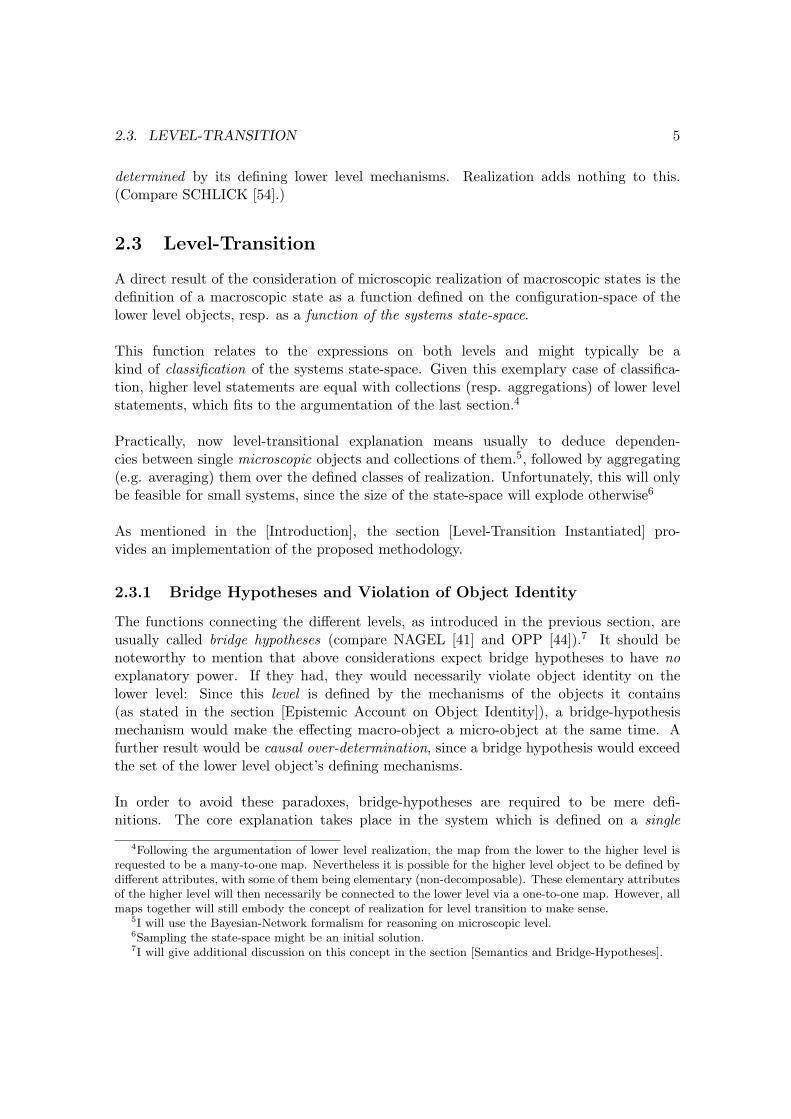
A direct result of the consideration of microscopic realization of macroscopic states is thedefinition of a macroscopic state as a function defined on the configuration-space of thelower level objects, resp. as a function of the systems state-space.
This function relates to the expressions on both levels and might typically be akind of classification of the systems state-space. Given this exemplary case of classifica-tion, higher level statements are equal with collections (resp. aggregations) of lower levelstatements, which fits to the argumentation of the last section.4
Practically, now level-transitional explanation means usually to deduce dependen-cies between single microscopic objects and collections of them.5, followed by aggregating(e.g. averaging) them over the defined classes of realization. Unfortunately, this will onlybe feasible for small systems, since the size of the state-space will explode otherwise6
As mentioned in the [Introduction], the section [Level-Transition Instantiated] pro-vides an implementation of the proposed methodology.
2.3.1 Bridge Hypotheses and Violation of Object Identity
The functions connecting the different levels, as introduced in the previous section, areusually called bridge hypotheses (compare NAGEL [41] and OPP [44]).7 It should benoteworthy to mention that above considerations expect bridge hypotheses to have noexplanatory power. If they had, they would necessarily violate object identity on thelower level: Since this level is defined by the mechanisms of the objects it contains(as stated in the section [Epistemic Account on Object Identity]), a bridge-hypothesismechanism would make the effecting macro-object a micro-object at the same time. Afurther result would be causal over-determination, since a bridge hypothesis would exceedthe set of the lower level object’s defining mechanisms.
In order to avoid these paradoxes, bridge-hypotheses are required to be mere defi-nitions. The core explanation takes place in the system which is defined on a single
4Following the argumentation of lower level realization, the map from the lower to the higher level isrequested to be a many-to-one map. Nevertheless it is possible for the higher level object to be defined bydifferent attributes, with some of them being elementary (non-decomposable). These elementary attributesof the higher level will then necessarily be connected to the lower level via a one-to-one map. However, allmaps together will still embody the concept of realization for level transition to make sense.
5I will use the Bayesian-Network formalism for reasoning on microscopic level.6Sampling the state-space might be an initial solution.7I will give additional discussion on this concept in the section [Semantics and Bridge-Hypotheses].
6 CHAPTER 2. LEVEL-TRANSITORY EXPLANATION AND EMERGENCE
level which will be the lower one, because of its higher informational content. (Furtherdiscussion of the topic can be found in section [Explicit Application of the Micro-Macro-Scheme].)
Nevertheless, bridge hypotheses are very important concepts in social science sincethey code assumptions on processes which cannot be considered in every detail. Theirinherent ontological paradoxy does not make them useless statements, as long it iscontrolled.
2.3.2 Proxy-Descriptions
Given that a description of the lower level process cannot be found, an aggregatedescription may certainly be used as a proxy for knowledge of the fundamental process.Practically, this will be necessary in most applications, typically for reasons of lacking data.
For this purpose an additional assumption will be necessary: Aggregate measuresof the system (as they can be gained economically by sampling) usually need to bebacked up with assumptions on structural homogeneity in order to serve as a proxyof the microscopic process. The assumption of homogeneity of unobserved structurescan be justified by an argument similar to OCKAHM’s Razor or LAPLACE’s Principleof Insufficient Reason, which applies in this case as follows; Structural homogeneity isthe simplest assumption as well as the expectation of random structures where everyparticular structure is assigned equal probability, because none can be preferred becauseof ignorance.
2.4 Reduction and Manipulation
By employing this methodology, level-transitional conclusions can be logically achieved,at the cost that the higher level seems merely more than a “useful manner of speech”,how SCHLICK [54] called it.
But this may be true for everything. The definition of mechanisms (and thereforeobjects) seems to depend on considerations on manipulation as causality might beregarded generally (compare BISCHOF [5], PEARL [47] and VON WRIGHT in SOSA etal. [61]).
Emphasized: Wether something is said to be an object might depend on our abilityto manipulate it.
Given this view, anything which can be attributed a use (a reason for manipula-tion) could be said to be possibly real. Usefulness seems to me to be the boundary ofinsight of reality: Given usefulness, logical coherence is just a means, depending on the
2.4. REDUCTION AND MANIPULATION 7
features of the objects and mechanisms in focus.
This is the reason why I do not propose reductionism as a general ontology. Ithas the advantage of logical coherence, but intuition of both logic and object identitymight be dependant on the needs of the human observer.
Assuming a level where it makes sense, while being reductionistically coherent onlyduring level transition might be a more practical approach.8
2.4.1 Hypothesis or Definition?
The above result may certainly seem peculiar from the viewpoint of Theory of Sciencein its tradition of Logical Positivism and Critical Rationalism. (Compare for exampleSCHNELL et al. [55] or SEIFFERT / RADNITZKY [56].) The reason for this is thatTheory of Science hides metaphysics (and thus ontology) in considerations on logicalstructures of theories.
For example, I might be expected to answer the serious question wether a bridgehypothesis is requested to be a “hypothesis”, in form of an implication, or a “definition”,in form of an equivalence.
Let me show the syntactic difference between those forms of propositions. In thecase of equivalence, both antecedent and apodosis of the proposition are fixed. Therecannot be any variation in it. In the case of implication, the antecedent is free and subjectto variation. The point is that this difference fits nicely to the ideas of metaphysicalinertness (for equivalence) and productivity (for implication). These concepts arenecessary for the question to make sense.9
Returning to above question on bridge-hypotheses, it now seems that I am askedto answer an ontological question and no formal one, although this is not explicit anyhow.Needless to say that empirical methodology, being coherent to logicism, adheres to adifferent concept of observation (and thus intelligibility of reality) than the one proposedin the section on [Reduction and Manipulation]. Therefore the question wether bridgehypotheses are expected to be “definitions” or “hypotheses” wether can only be answeredby regarding to the mentioned metaphysical considerations. The answer in my terms
8The pragmatic argument does not mean that I deny reality and truth or the need for ontology: it fitsto the idea of manipulation being the substrate of causality and is furthermore epistemologically ratherstraightforward, as compared to the stronger criterion of correspondence between proposition and reality.More of this in the section on [Aspects of Modelling].
9I just want to remark that definitions and hypotheses do not necessarily need to be represented by thetwo mentioned constructs. Every computer program employs directed assignment-operators rather thanequivalences for representation of definitions. Syntax is simply a question for the range of its coherencewith semantics. As long as it works, it works. (Compare section [Aspects of Modelling].) Similar argumentis employed by BUNGE [7] in order to attack RUSSEL’s proposition of differential equations being theonly possible formulation of natural laws.
8 CHAPTER 2. LEVEL-TRANSITORY EXPLANATION AND EMERGENCE
is, that I request inertness being an attribute of bridge-hypotheses, but this does notnecessarily deny productivity on a specific level. (Compare [Reduction and Manipulation].)
According to a metaphysics of correspondence between proposition and reality, forexample Logical Positivism or its successor Critical Rationalism, this ambiguity wouldbe senseless and contradictory. But it is not for a weaker metaphysics of Pragmatism asadvocated in section [Aspects of Modelling].
2.5 Emergence
My preceding arguments concerning level-transitory explanation were based on an epis-temic definition of the objects discussed. This now allows for an account on emergence,which is also indecisive regarding ontology.
The previous problem took the higher level for predefined, which is obviously notthe case for emergence. Consequently, the task consists in defining its criterion in a waythat it can coherently serve as input for my approach to the problem of level transition.This instantly yields in the following proposition: Collections of objects should beattributed emergent properties if they behave autonomous (see above) on at least aconceptual level.10
This is the case if the system or subsets of its elements exhibit self-regulation orself-organization. The first means that the system compensates for outside disturbances(BISCHOF [5]) while the second can bee seen as the tendency of a system to reach certainsteady-states (BERTALANFFY [4]) given a certain range of environmental conditions.Both phenomena have in common that usually only a subset of the possible state-spaceis realized, and that this realized states are functional (partial probability-increasing)towards themselves (as mentioned) given a certain range of environmental conditions.
Now, by following the argumentation of the last section, I will define emergentproperties as classification11 of the auto-functional subsets of the systems state-space.
It is to be mentioned that this is no ontological definition of emergence, since itbuilds again on the concept of perceived autonomy. I just turned the direction ofargumentation, compared to the approach to level transition: Self-regulation andself-organization are strong grounds for the attribution of autonomy.
In order to conclude the discussion of emergence, I should emphasize the fact thatI am neither discussing properties of the auto-functional subsets of the systems statespace nor the process of reaching them. The question of steady states and derivation of
10With regard to systems, autonomy is encoded by definition of the systems boundary. (Compare[System].)
11Or more generally as a function.
2.6. REMARKS ON COMPLEXITY 9
emergent properties is beyond the scope of this project12, although I am very interestedin it.13
2.6 Remarks on Complexity
An argument from the emergentist part of Philosophy of Mind, is denial of the possibilityof microscopic modelling because of extremely complex patterns of “wild disjunction”of the possible instantiations of a macro-state, as advocated by SAWYER [51] [52] andmentioned by HEINTZ [20].
This argument is certainly challenging, but I will only give a short reply. Thanksto the possibility to cope with multiple dependencies granted by the use of probabilitytheory, the “complexity” (e.g. difficult decomposability with respect to both structuresand mechanisms)14 of a system is not a problem anymore.15 The problem remains itssize.
If “wild disjunction” is interpreted before this background, a possible approach tosolve this problem may be investigating the structure of the auto-functional subsets ofthe state-space, as defined in the emergence-section, for instance by considerations aboutthe evolutionary advantage (e.g. functionality) of hierarchical structures defined on thesystems components as done by SIMON. [59] [60]
Allow me a final remark: I guess that complexity, in a sense of exhausting humanconception, may be responsible for occurrence of the question on levels. If we are facedwith systems that are simple enough to be elementarily described, no one expresseshis considerations in terms of levels. This becomes an option, when systems begin torefuse revealing information on their elementary processes and a gross-treatment becomesnecessary for understanding. 16
12One could say, that a practical solution of this questions (or simply a definitory bypass) is a prerequisitefor the epistemic approach on level transition.
13I only can recommend literature at the moment: the work of STEGMUELLER [62] provides anexcellent general account on self-regulation, while the work of BISCHOF [5] is extraordinary, both withrespect to teaching (it introduces time-discrete control-theory and information theory) and fundamentalresearch (it describes a method for defining semantics on evolutionary systems without having to invokeintentionality). The works on General System Theory of BERTALANFFY [4] and Hierarchical Systemsby SIMON [59] [60] can be considered classical. Right now, NICOLIS’ and PRIGOGINE’s book [43] onDissipative Systems is on my bed table, but I will not finish it before delivering my thesis.
14This use of complexity is not necessarily isomorphic with the information-theoretic use of the word,where Kolmogorov-Complexity designates the informational content of a signal by referring to the lengthto the shortest program capable to produce that signal. This measure of complexity can be said to answerthe question how complicated a possible “explanation” of the signal might be. Im not deep enough intothis particular problem in order to treat it employing mathematical notions, but nevertheless the ideashould become clear.
15This is discussed in the “Mathematics”-section16This certainly does not mean that the lowest level of consideration is necessarily “real”. Confounding
of the conception of being with the conception of manipulation may be true for every level.

10 CHAPTER 2. LEVEL-TRANSITORY EXPLANATION AND EMERGENCE
Chapter 3
Aspects of Modelling
Now I want to introduce the notions of model and model-calculus, followed by some con-siderations about modelling as a scientific methodology. 1
3.1 Model
A model is essentially a map, but with certain characteristics: there exists 1. a so calledtarget set2 which is the system of interest, and 2. a so called image- resp. model set, intowhich the map proceeds. The discriminating point is the intelligibility, or more generalusefulness of the image set compared to the target set. This is the reason for buildingmodels.
Furthermore, target- and image set can be compared with respect to their compo-sition: the subset of elements of the target which is not represented in the image is calledpreteriton-class of the model-relation, while the subset of elements of the image whichhave no complement in the target is called abundance-class (see TROITZSCH [65]). Thiscomparison is very interesting, because it shows the limitations of the model with regardto its “original” and therefore allows to investigate the actual relation between target-and model set.
3.2 Model-Calculus
Perhaps the most exciting and useful models are mathematical models. These are definedby the fact that the image set is a subset of a domain of a calculus. I will call thiscalculus operating on the image set of a model-relation model-calculus. A different way ofarticulating this is to say that the model-relation defines a semantic on the calculus (seeCARNAP [9]).
1I apologize for introducing the method of modelling this late, although its omnipresence within thiswork. It is still abstract enough, I guess.
2The direct mathematical translation would be preimage, which is a little bit cryptic for our purposes.
11
12 CHAPTER 3. ASPECTS OF MODELLING
The employment of a model-calculus allows 1. for “automatization” of the imageset by providing rules of computation and 2. proving assumptions about the generalbehavior of the image set.
Certainly, a model-calculus may be hard to understand, but work invested here willpay off: large problems will not be resolved without automatization while complicatedproblems are longing for exactly defined semantics.3
3.3 Modelling as a Mindset
The advantages of modelling as an approach to science consist of flexibility and creativity.Since it is not imperative to generalize the applicability of the image set and its associatedcalculus beyond the scope of the target set, one is free to choose syntax and semantics(or resp. the kind of model) according to demands of the problem and the simplicityof the own mind. Certainly, gain of generality is not hindered by this approach, sincegenerality is a hallmark of good theory. But nevertheless, applicability seems to benecessary criterion of a theory which corresponds to reality.
Applicability will be my central criterion for a good model, besides generality andsimplicity. Generality as a result of abstraction might well be demanded from a model ofcomplex processes. Therefore the claim for simplicity can be justified by considerationsregarding the own mental capabilities, as implied above.4
This “ethical” argumentation may sound inadequate to the subject. But even if itlooks differently, I am a believer with regard to synthetic truth. But I will not talk aboutjustification of the genuine truth of my models, given they are of limited use for mypurposes.
This criterion is weaker than for instance the most elaborate criterion of CriticalRationalism as posed by LAKATOS [30]. But it allows thought to flow more freely thanthe latter. I hold a similar attitude towards structuralism (see STEGMUELLER [63] orTROITZSCH [65]). Rational reconstruction of a domain of knowledge may be of greatestvalue, granted that there is already enough substance within this domain of knowledge.My claim regarding acquisition of this substance is: One needs to dare new theory.5
3This is often not the case with MABS.4One could also say that the two lower criteria flow from applicability by invoking stupidity and laziness.5Certainly there is much more to know in the field of Theory of Science. Nevertheless, one thing is
never treated: the need for decision. The idea of truth contains too much ambiguity to give us specificorders.
Chapter 4
A Sketch of Bayesian Networks
During this section I will briefly introduce the employed mathematical apparatus.
4.1 Sketch of the Method
While I proposed in the philosophy-section that level-transitory explanation can beaccomplished by aggregating dependencies between single microscopic objects andcollections of them, it remained unclear how these dependencies should be modelledand deduced; especially, when the structure of dependency is rich but incomplete. Thisquestion has been approached with the technique of bayesian networks.
In principle, the bayesian network formalism is a special formulation of probabilitytheory. The basic idea is as follows: By employment of the fundamental theorem ofprobability calculus, a joint probability distribution is decomposed into a graph, resp.a network. The nodes of this network represent the marginal distributions of the setof random variables in question, while the edges connecting the graphs nodes representconditional probability distributions1.2
It should be furthermore important to note, that although being named “bayesian”, theformalism is not necessarily connected with a bayesian3 interpretation of probability asprovided by the Cox-Jaynes-Axioms (BALDI / BRUNAK [3]: p.50 and JAYNES [24]). 4
The name “bayesian network” rather stems from the use of Bayes Theorem for abductive5
reasoning: While PEARL [47] advocates a bayesian standpoint, JENSEN [25] applies aclassical frequentist definition of probability.
However, the application of probability theory and especially bayesian networks to
1Actually, this is often called a “Graphical Model”.2A good introduction to bayesian networks is JENSEN [25].3Which reads subjectivist, non-frequentist.4Although I am an enthusiast regarding bayesian theory, I will abstain from an introduction.5Abduction is the inversion of deduction: A ⇒ B, B is there, therefore A is more plausible;
13
14 CHAPTER 4. A SKETCH OF BAYESIAN NETWORKS
the problem is due to several advantages
• probability theory naturally allows inferring arbitrary dependencies between thevariables considered, while taking account of multiple dependencies and even mul-ticausality6 (see JAYNES [24] and PEARL [47]). Usually, mathematical modelswhich are deducing macroscopic statements from microscopic theory are ignoringstructures of interdependence. Examples are the synergetic model of attitude for-mation by TROITZSCH [65], [67] and COLEMAN’s [11]: pp.241 model of politicalactivity.
• Bayesian Networks allow for a rather convenient representation of systems: sincethey can be modelled via local distributions (the nodes) and their probabilistic de-pendencies (the edges), only knowledge on the elementary level is necessary. Inshort, they naturally allow for microscopic modelling.7
• With respect to Multi Agent Based Simulations (MABS)8 (see GILBERT /TROITZSCH [16], WEISS [69] and CONTE et.al. [13] for introduction), bayesiannetworks have the advantage that they operate on a carefully defined mathematicalstructure. This allows to clarify the relations between notions of the content-orientedtheory and the mathematical one, which is very important for interpretation of mod-els. I should add, that although lacking mathematical rigor (as mentioned) MABSeasily allows for the modelling of structured dependencies.
• Bayesian Networks can be easily integrated with empirical data, as it is generallytrue for probability theory.
All these advantages certainly come at a cost. The cost is computer-memory and lackof speed.9Models easily become intractable, which makes simulation and MABS a betterchoice for investigating their middle and long term behavior.10
So much for introduction of the technique and back to the question of inferringdependencies between single objects and collections of them in systems with incompletestructure of dependency.
Bayesian networks allow to calculate and express these dependencies in form of aconditional probability distribution. What is left to do after computing the conditional
6The mode of inference in a probabilistic model is insensitive to hazards like structured independenceand nonlinearity: it is basically summation, resp. integration.
7I hold the view that probability is no ontic “force”: it rather stems from ignorance. And since I havegot enough of this, I may add a flavor of it to all of my models.
8Swiftly spoken, MABS model a system by representing its lower level entities as interacting softwareobjects.
9I experimented with a Dynamic Bayesian Network with twelve variables per time-slice, which couldonly be solved approximately by sampling techniques like Likelihood-Weighting in my case.
10MABS and bayesian networks could certainly be combined with the latter being an analysis tooloperating on model generated data. During the course of this work this proved to be preferable comparedto direct modelling. Compare [Model Sensitivity].
4.2. DEFINITION OF BAYESIAN NETWORKS 15
probabilities (which connect the realizations of a macro state with the single elementstate) is aggregating.
4.2 Definition of Bayesian Networks
After above informal introduction to bayesian networks, I will additionally provide aformal one.
First, I will briefly review some basic concepts of probability theory11. Then I willgive an introduction to the concepts necessary for building bayesian network models. Forthis reason I will not talk about many details and especially the treatment of inferencealgorithms.12
4.2.1 Decomposition of Joint Probability Distributions
The first concept I want to mention is the concept of a joint probability distribution.This is a mathematical structure, where every joint occurrence of elements of a set ofstatements is attributed a probability.
In frequentist thought, the joint probability distribution is the structure which codes aprobabilistic model and the most natural way of defining such a model is to generalizeobserved frequencies of the variables in focus towards probability. Given this view, therelationships between the elementary statements within the joint probability distributionare defined by the Fundamental Theorem of Probability Theory:
P (a|b) =defP (a, b)P (b)
(4.1)
The mentioned relationship is certainly a conditional probability. As can be seen, thisconditional probability is defined in terms of joint- and marginal probabilities, which bothcan be easily gained by measurements of frequency. Certainly I can manipulate the formulain order to gain:
P (a, b) = P (a|b)P (b) (4.2)
This equation shows the equivalence of the joint probability with a product of aconditional- and a marginal probability.13 This formula can certainly be extended fora joint of more than two variables, which leads to the Chain Rule:
11For a complete introduction, the reader may be referred to the works of JAYNES [24] and LARSON[31], where the first is rich on philosophy and advocates a bayesian approach and the latter is a compactintroduction to classical theory.
12For a sound contact to the topic the reader is referred to BALDI / BRUNAK [3], JENSEN [25] andPEARL [46] [47].
13The asymmetry in above definition (eq. 1) reflects a frequentist account to probability theory, demon-strated for convenience of the reader.
16 CHAPTER 4. A SKETCH OF BAYESIAN NETWORKS
P (x1, ..., xn) =∏
j
P (xj |x1, ..., xj−1) (4.3)
Applying the Chain Rule allows for the decomposition of a joint probability distributionas a product of conditional- and marginal distributions.
This immediately results in the following semantic advantage: Now the system ofvariables in scope can be described by their marginal distributions (as elementary prop-erties) and their relationships in terms of conditional probabilities. So to speak, globalprobabilistic propositions can be decomposed into local ones.
4.2.2 Graphs and Conditional Independence
Within the Chain Rule, indirect relationships between variables are represented explicitly.This prohibits the design of a “wiring scheme” (or network model) of the system, sinceit would contain unnecessary connections between the marginal distributions. This canbe avoided by accounting for conditional independence14 of the considered variables: Twovariables X and Y are said to be conditionally independent given Z if
P (x|y, z) = P (x|z) whenever P (y, z) > 0 (4.4)
Given, that our network model should map the directions of the relations 15and shouldfurthermore contain no cycles16, we can find the set of prior variables in this networkwhich makes a certain variable xj independent of all its other predecessors . This set iscalled Parents of xj or paj . To eliminate all indirect connections towards xj out of thedirected and acyclic network, the Parents of xj need to satisfy the following condition:
P (xj |paj) = P (xj |x1, ..., xj−1) for all x1, ..., xj−1 prior to xj (4.5)
This is the Markov-Parentship-Criterion17 for directed acyclic graphs or DAGs18, howsuch a “wiring scheme” is called.
The Parentship-Criterion can easily be applied to the Chain Rule. This finally al-lows for the decomposition necessary for local representation of a joint probabilitydistribution by a directed acyclic graph by invoking the Chain Rule for BayesianNetworks:
14More implications of conditional independence can be found at PEARL [47]:p.11, “Graphoid Axioms”.15Usually one has to decide on the ordering of the variables by causal intuition. Nevertheless there exist
methods to extract causal orderings form data. PEARL [47]16This is imperative for reasoning. Schematics which allow for cycles (like for instance block diagrams
in Control Theory) are implicit with respect to the order of computations, resp. time.17The Markov-Parentship-Criterion is a way to define the autonomy, resp. isolatability of an object with
respect to certain,a priori known properties, as mentioned in the section [Epistemic Account on ObjectIdentity].
18A more formal definition of a DAG will follow in the next section.
4.2. DEFINITION OF BAYESIAN NETWORKS 17
P (x1, ..., xn) =∏
i
P (xi|pa(xi)) (4.6)
This equation, together with the prerequisite of representation of the conditionalindependence-relations between the marginal distributions via a DAG defines a bayesiannetwork.
4.2.3 Inference in Bayesian Networks
Reasoning in Probability Calculus consists basically of projecting a joint probability dis-tribution down to subsets of it: may that be joints, marginals or conditional probabilities.
So, the joint probability of two variables (Y,X) can be projected towards the probabilityof the occurrence of a certain value yi of the variable Y by summing over the values of X:
P (yi) =m∑
j=1
P (yi, xj) (4.7)
This is also called marginalization and is denoted the following way, if applied to distri-butions:
P (Y ) =∑
X
P (Y, X) (4.8)
conditional probabilities can be accessed by employing both fundamental theorem (eq. 1)and marginalization:
P (y|x) =∑
s P (y, x, s)∑y,s P (y, x, s)
(4.9)
A strength of Probability Calculus can be seen in the natural ability of performingabductive reasoning19 efficiently. The inversion of a conditional probability is accomplishedby Bayes Theorem:
P (y|x) =P (x|y)P (y)
P (x)= L(x|y) (4.10)
The inverted conditional probability is often called likelihood.
Given that we gain evidence on the Values of some Variables within the network20,we may wish to calculate the now unknown marginal resp. joint distributions on theremaining variables (which would yield conditional distributions in both cases). In short,
19As mentioned before, abduction is the inversion of deduction: A ⇒ B, B is there, therefore A is moreplausible;
20“Evidence” means to select a category of some variable with probability p=1, respectively to look onlyat the part of the joint probability distribution which accords to what we learned about the actual stateof this variables.

18 CHAPTER 4. A SKETCH OF BAYESIAN NETWORKS
we might like to employ this knowledge in order to calculate the total effect of theevidence, considering the structure of interdependence of the system of hypotheses inscope . We could use above techniques to yield the results of interest.
But as mentioned, a necessary prerequisite for all computations but for abductivereasoning is access to the joint probability distribution. This may only be the case in themost seldom cases, since it grows exponentially with the number of variable values.
Thus the local representation by a bayesian network allows for the employment oflocal computations in order to gain results which may be intractable by commonmethods. This is accomplished by the various inference algorithms for bayesian networks.Since efficient calculation with probability theory is a highly complicated matter, thediscussion of the several inference algorithms might exceed my capabilities. For moreinformation the reader is referred to PEARL [46], JENSEN [25] and GILKS et.al. [17].
Chapter 5
Probabilistic System Model
Since it is necessary to feed the machinery of probability calculus in order to get a run-ning model, it might be helpful to formally declare the actual model-relation.1 This willbe accomplished by introducing BUNGE’s general definition of a system. Relating thisdefinition to bayesian networks, I will gain the definition of a probabilistic system modelwhich can be processed by probability calculus.
5.1 System
Usually, a system is conceived as a set of interacting elements2, which might be in ourcase systems of individuals, collectives or institutions.
The eminence of the concept of system resides in the fact that it allows to repre-sent a higher level entity in terms of its constituting lower level entities. It seems tobe a natural container of the concept of perceived autonomy (see [Epistemic Accounton Object Identity],[Level Transition] and [Semantics and Bridge Hypotheses]), whosedomain is given by the systems boundary.3
In accordance to BUNGE [6] I will formally define a system St at time t by thetriple of the sets of its components Ct, the bonding relations Bt between its componentsand its environment Et.
St = 〈Ct,Bt, Et〉 (5.1)
With the lists of the systems components, bonding relations
Ct = {ct,1, ct,2, ...ct,n} (5.2)
1Another saying is that we declare a semantic on probability theory.2A well known exception are the infernal works of LUHMANN, like [35].3Nevertheless, for a complete level transition there is the need for translation of the notion defined on
the respective levels.
19
20 CHAPTER 5. PROBABILISTIC SYSTEM MODEL
Bt = {bt,1, bt,2, ...bt,m} (5.3)
and the components of the environment4, where the latter might often be condensed toein, the source of environmental input and eout, the sink of the systems output.5
Et = {et,1, et,2, ..., et,o} 7→ ECt = {et,in, et,out} (5.4)
I just want to mention that these components may be as well elementary objects, un-bounded sets of objects or systems itself. A subsystem SS may be defined by havingsubset relations of system S with regard to its composition set C and its bonding set Bwhile having superset-relations with regard to the environment set E .
SSt is a subsystem of St iff (CSt ⊆ Ct)&(BSt ⊆ Bt)&(ESt ⊇ Et) (5.5)
5.1.1 Graphical Representation
Systems can be modelled by a graph6 Gt whose nodesNt represent the union of componentsset Ct and the environment set Et
7 while its bonding set Bt maps8 to the set of edges EGt.
Gt = 〈Nt, EGt〉 (5.6)
given
Nt = Ct ∪ Et (5.7)
and
Bt 7→ EGt (5.8)
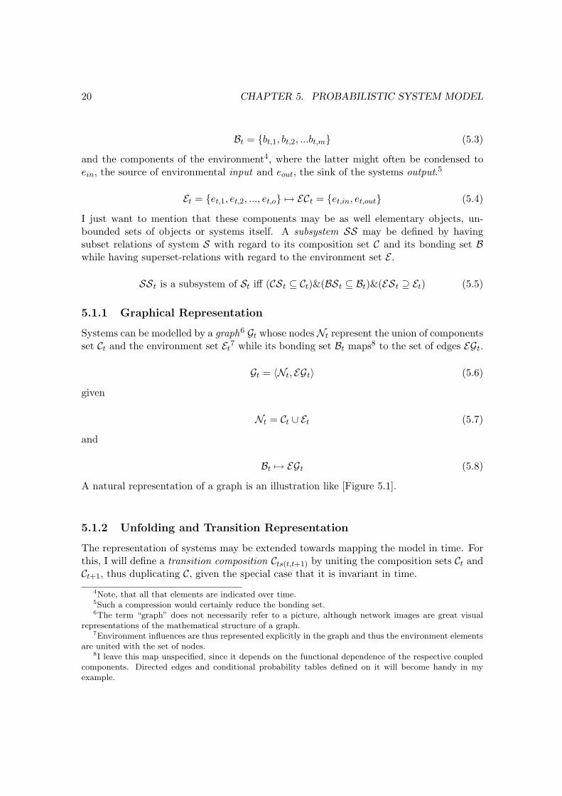
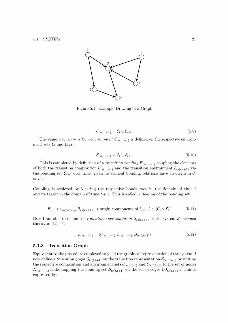
A natural representation of a graph is an illustration like [Figure 5.1].
5.1.2 Unfolding and Transition Representation
The representation of systems may be extended towards mapping the model in time. Forthis, I will define a transition composition Cts(t,t+1) by uniting the composition sets Ct andCt+1, thus duplicating C, given the special case that it is invariant in time.
4Note, that all that elements are indicated over time.5Such a compression would certainly reduce the bonding set.6The term “graph” does not necessarily refer to a picture, although network images are great visual
representations of the mathematical structure of a graph.7Environment influences are thus represented explicitly in the graph and thus the environment elements
are united with the set of nodes.8I leave this map unspecified, since it depends on the functional dependence of the respective coupled
components. Directed edges and conditional probability tables defined on it will become handy in myexample.
5.1. SYSTEM 21
12
3
4
5
6
Figure 5.1: Example Drawing of a Graph
Cts(t,t+1) = Ct ∪ Ct+1 (5.9)
The same way, a transition environment Ets(t,t+1) is defined on the respective environ-ment sets Et and Et+1.
Ets(t,t+1) = Et ∪ Et+1 (5.10)
This is completed by definition of a transition bonding Bts(t,t+1) coupling the elementsof both the transition composition Cts(t,t+1) and the transition environment Ets(t,t+1) viathe bonding set Bt+1 over time, given its element bonding relations have an origin in Ct
or Et.
Coupling is achieved by locating the respective bonds root in the domain of time tand its target in the domain of time t + 1. This is called unfolding of the bonding set.
Bt+1 7→unfolding Bts(t,t+1) | ( origin components of bi,t+1) ∈ (Ct ∨ Et) (5.11)
Now I am able to define the transition representation Sts(t,t+1) of the system S betweentimes t and t + 1.
Sts(t,t+1) = 〈Cts(t,t+1), Ets(t,t+1),Bts(t,t+1)〉 (5.12)
5.1.3 Transition Graph
Equivalent to the procedure employed to yield the graphical representation of the system, Inow define a transition graph Gts(t,t+1) on the transition representation Sts(t,t+1) by unitingthe respective composition and environment sets Cts(t,t+1) and Ets(t,t+1) to the set of nodesNts(t,t+1)while mapping the bonding set Bts(t,t+1) on the set of edges EGts(t,t+1). This isexpressed by:
22 CHAPTER 5. PROBABILISTIC SYSTEM MODEL
Gts(t,t+1) = 〈Nts(t,t+1), EGts(t,t+1)〉 (5.13)
with
Nts(t,t+1) = Cts(t,t+1) ∪ Ets(t,t+1) (5.14)
and
Bts(t,t+1) 7→ EGts(t,t+1) (5.15)
5.1.4 Representation in Time: Temporal Graph
Graphical representation of the system in time is gained by definition temporal graphGtemp(t:t+n) representing the system from time t to time t + n by concatenation of thetransition graphs Gts(t,t+1) to Gts(t+(n−1),t+n). Given indication of the systems sets overtime, this is accomplished by uniting the respective transition graphs.
Gtemp(t:t+n) = Gts(t,t+1) ∪ Gts(t+1,t+2) ∪ ... ∪ Gts(t+(n−1),t+n) (5.16)
If the structure of the transition graph does not change over time, one could say that thetransition graph is unrolled in time.
5.2 Bayesian Network Representation
Now I want to apply the results of the last subsections to the problem of defininga bayesian network on the system. The first conclusion is that the temporal graphGtemp(t:t+n) can be used to define the structure of a bayesian network modelling systemover time, given that its edges are directed. Such a temporal bayesian network is usuallycalled a dynamic bayesian network, although time is represented explicitly.
We need to define the conditional probability distributions attached to the edges.Recalling the chain rule for bayesian networks
P (n1, ..., nn) =∏
k
P (nk|pa(nk)) (5.17)
We identify the term nk|pa(nk) with the subset EGpa(nk) ⊆ EGtemp(t:t+n) of the set ofedges of the temporal graph Gtemp(t:t+n) which point towards the node nk, given that theindex k is a mapping of the time-explicit indication introduced in the [System]-section.
EGpa(nk) = EGtemp(t:t+n) |(egj pointing towards nk) ∈ Ntemp(t:t+n), nt,i 7→ nk (5.18)

5.2. BAYESIAN NETWORK REPRESENTATION 23
What finally needs to be mapped is the bonding information BI exceeding the defi-nition of the existence and direction of edges on the conditional probability distributionP (nk|pa(nk) attached to EGpa(nk).9
BI(EGpa(nk)) 7→ P (nk|pa(nk) (5.19)
This map can be arranged by either theoretic deduction of the probabilistic relationbetween the components in scope, or by learning the relationships from data (seeBALDI/BRUNAK [3] and PEARL [47]).
Finally, if the joint probability distribution can be composed by invoking the chainrule for bayesian networks, the formulation of a probabilistic system model is achieved.
9As remarked in the section on [Graphical Representation], the map from elementary to graphicalrepresentation was left unspecified because of the implicitness of the actual functional dependence betweenthe elements of the system. The bonding information BI is exactly the explication of this unmappedfunctional dependence.

24 CHAPTER 5. PROBABILISTIC SYSTEM MODEL
Chapter 6
Methodological Individualism
Now, after having introduced the foundations of level transitory modelling, I will discussmy philosophical approach to the problem of level-transition in relation to its widespreadequivalent in the social sciences, the Coleman Micro-Macro-Scheme (COLEMAN [12]). Ishould note that although it is named after James COLEMAN, its first occurrence can befound in McCLELLAND’s “The Achieving Society” [36]1.
6.1 The Micro-Macro-Scheme and Methodological Individ-ualism
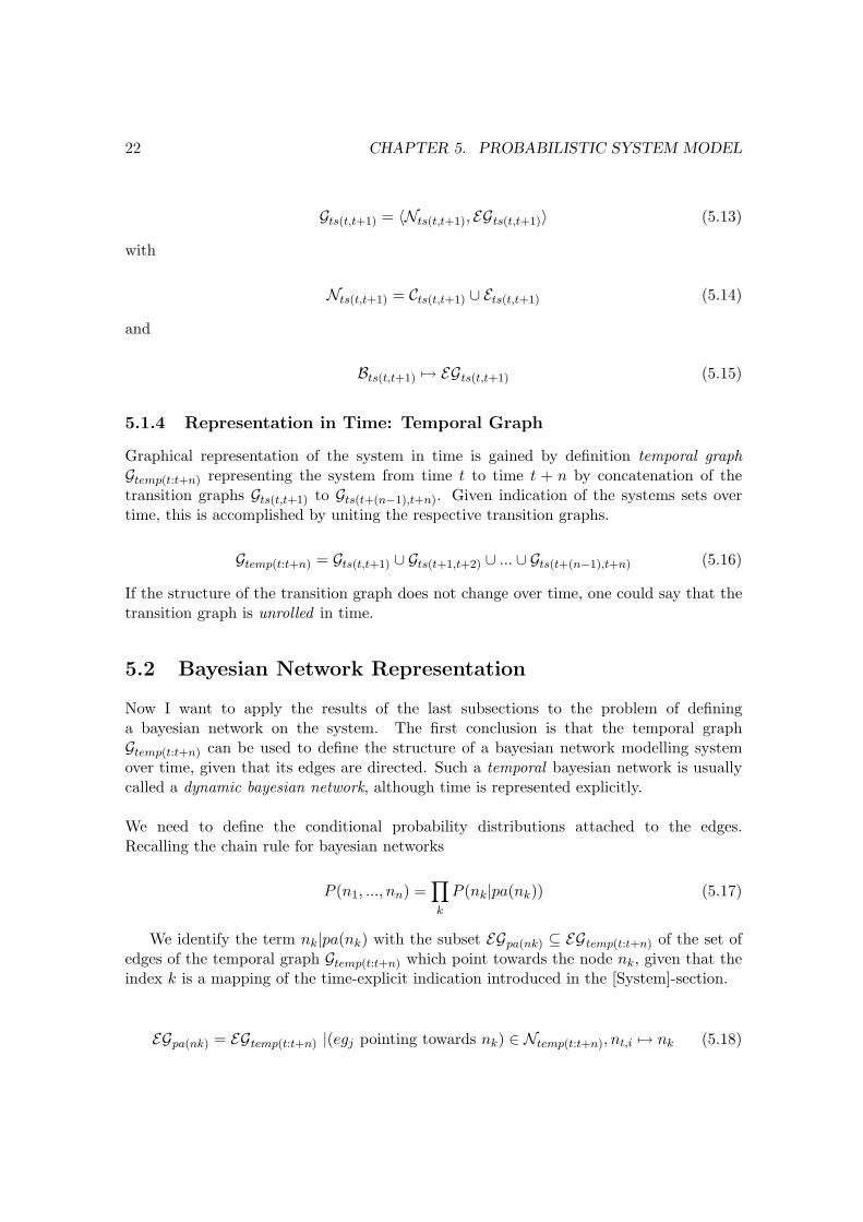
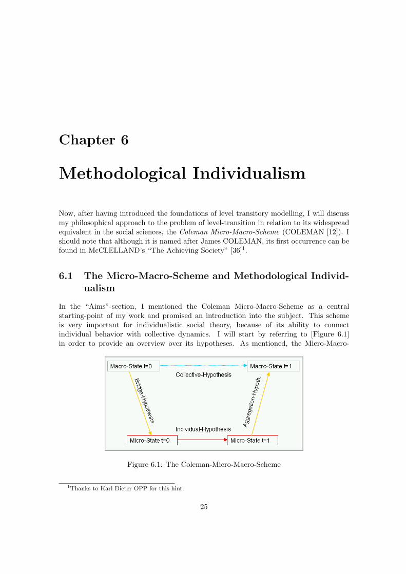
In the “Aims”-section, I mentioned the Coleman Micro-Macro-Scheme as a centralstarting-point of my work and promised an introduction into the subject. This schemeis very important for individualistic social theory, because of its ability to connectindividual behavior with collective dynamics. I will start by referring to [Figure 6.1]in order to provide an overview over its hypotheses. As mentioned, the Micro-Macro-
Figure 6.1: The Coleman-Micro-Macro-Scheme
1Thanks to Karl Dieter OPP for this hint.
25
26 CHAPTER 6. METHODOLOGICAL INDIVIDUALISM
Scheme can best be described as a typology of the hypotheses necessary to accomplisha level-transitory explanation. The hypotheses substituting the collective (or macro-)hypothesis during individual-based explanation can be classified as Bridge-Hypothesis2,Individual-Hypothesis (resp. Action-Hypothesis) and Aggregation-Hypothesis.
Before examining these hypotheses in detail, I want to discuss the main assump-tions of this scheme. The first assumption is certainly systemicity of the social realm,or in other words, that a social entity is a composite of lower level entities. Thesecond assumption is, that the lower level entities are persons which are connected bytheir respective actions. This is the founding assumption of so called “MethodologicalIndividualism”.
6.2 Explicit Application of the Micro-Macro-Scheme
You wont be surprised to read that there is much discussion concerning the notionof Methodological Individualism. There exist several attempts to formulate it, orrespectively its most usual formulation, the Micro-Macro-Scheme, in a way that allowsfor the occurrence of emergent properties.
A short excursion to the actual practice of level transitory explanation may benecessary to clarify the associated problems.
One frontline is the question how the Individual-Hypotheses should be instanti-ated, 3 which certainly shifts the focus from level-transition to microscopic theory andeffectively relabels the problem while displacing it into the particular instances of themicroscopic theories. Following this tradition, a level-transitory-explanation consists ofdetermining the initial-values of the microscopic hypotheses, deducing their consequencesand averaging the results. This way, the separate hypotheses of Micro-Macro-Scheme areapplied one-to-one. A good introduction of this procedure can be found at OPP [44].
The interesting point is, that a microscopic approach to level transition, (as de-signed in the respective section) can certainly be interpreted as an implicit version of thisprocedure. The reason for this is that a systems state can certainly be interpreted asinitial condition for the components mechanisms.
Nevertheless, a conventional approach which tries to instantiate the Micro-Macro-
2More on this type of hypothesis in the sections [Level Transition] and [Semantics and Bridge Hypothe-ses].
3This discussion can be followed in past issues of “Koelner Zeitschrift fuer Soziologie und Sozialpsy-chologie” (KZFSS). The adversaries, all members of the “Rational-Choice” enterprise, consisted of LIN-DENBERG [33], [34] and ESSER [15], who advocate a theory-driven microeconomical approach, and onthe other hand KELLE and LUEDEMANN [27], [28] and OPP and FRIEDRICHS [45] who are more proneto an empirico-statistical paradigm similar to those of empirical social research. A recent contribution tothe subject is given by DAVIDOV / SCHMIDT [14].
6.3. MACRO-STATES AND INITIAL CONDITIONS 27
Scheme by trying to explicitly conclude with its classes of hypotheses is logically ormethodologically flawed. This is because of two reasons which already have beenintroduced in the section on [Level-Transitory Explanation and Emergence]:
First, an elementary (which reads “not composite”) description of a macroscopicstate is inconsistent with the idea of a composite system, which is constituting for theproblem of level-transition. A elementary description of higher level entities can not beuninformative in the sense defined in the section on [Bridge Hypotheses and Violationof Object Identity]. Therefore coherence of object identities on both levels, which isimperative for reasoning, cannot be maintained in this case. Certainly making thisproblem implicit by shifting it into discussions about initializations of SEU-Theory willnot solve it.4 Discussion of this topic is given in the next section.
And second, a map from notions of composite system structure to notions of macroscopicstates is many to one- and therefore not invertible map. Because of this syntacticallyelementary5 description of a systems macroscopic state lacks the possibility to map itsstructure and is therefore only feasible for structureless phenomena. (These seemed todeliver a template for microscopic modelling until recently.6) A technique which copeswith more complicated phenomena is required to map the relevant structure of thesystem. This further disqualifies the one-to-one application of the Micro-Macro-Schemeto many cases of interest.
6.3 Macro-States and Initial Conditions
It can be easily seen, that my arguments in the last section attacked merely a methodof defining initial-values for an individual hypothesis, and not the individual hypothesisitself. This is not accidental since the research programme of the Sociology of RationalChoice identifies the Subjective Expected Utility (SEU) Hypothesis as its very core.(Compare for instance COLEMAN [12] and KELLE/LUEDEMANN [27].)
Shifting the question of macroscopic properties and emergence into the initial con-ditions allows to shield the individual hypotheses of the joint theory from doubt, resp.
4The discussion about theoretical “richness” or “abstinence” of bridge-hypotheses, as discussed inKZFSS, is an example for this. Focus of argumentation is the question how to gain valid instances ofSEU, and not how to bridge levels.
5In the sense of CARNAP [9], who distinguishes between “elementary” and “complex” formulae andnotions, an elementary notion is one that cannot be decomposed within a given system of axioms.
6Possible examples are so called “Mean-Field-Models”. Since a mean is the “balance point” of a distri-bution, all its values can be understood as to be balanced against each other. The structure of interactionis treated as complete, which avoids the necessity for a detailed view on the lower level process. Themodels of TROITZSCH [65], [67] and COLEMAN [11]: pp.241 show such a characteristic, as mentioned.Although I am advocating structural modelling in this work, I have to confess that assumptions of struc-tural homogeneity might be necessary for the most real problems. One needs to work with the data onecan get and I would not trow away useful methods like HLM or Bayesian Hierarchical Models. Detaileddiscussion is given in section [Proxy Descriptions].

28 CHAPTER 6. METHODOLOGICAL INDIVIDUALISM
from the problems associated with level-transitory explanation.7
A striking example for the synonymous use of “Macroscopic State” and “InitialCondition” is OPP’s ([44]: p.90-105) introduction to the subject. He tries to explainthe disintegration of a public audience by application of the macro-micro-scheme: Rainpouring on the audience is defined as “collective attribute” and employed to initialize theindividual process of decision, wether to stay or to leave.
Certainly, “absence of rain” is no constituting property of a public audience. Situ-ations are simply taken for collectives. Rightfully, I should note that OPP shares thiserror with his theoretical adversaries LINDENBERG [33] and ESSER [15], as well aseventually with DAVIDOV and SCHMIDT [14].
6.3.1 Semantics and Bridge-Hypotheses
Certainly the synonymous use of “bridge hypothesis” and “initial condition” avoidscontact with the actual problem of level transition. I will now discuss that problem withregard to the definitory “delicateness” of bridge-hypotheses.
As far as I know, the term “bridge hypothesis” was coined by NAGEL before thebackground of explaining one theory via another, denoting a hypothesis which relates (ortranslates) notions of the different theories (Compare NAGEL [41] and SCHEIBE [53].).It should be furthermore noticed that NAGEL’s argumentation proceeds on a level oftheoretic statements .8
In our case, the problem faced in the attempt of reduction consists in deliveringdefinitions on the objects and properties defined on the different levels which aresemantically consistent and allow for conservation of object identity on both levels. Thisimplies the coherence of the respective definitory models on both image- (as postulatedby NAGEL) and preimage / target - level.
This coherence can be gained by introducing a third model, which maps the rela-tions between the preimage-sets on both levels. In my case the (rather implicit) modelis a theory of knowledge and modelling which results in the assumption of perceivedautonomy of objects. This assumption connects the “designata” on both levels.
I should mention, that in my view this discussion is usually no issue in scienceswhich employ the notion of a system rather than of higher level entity. The notion ofsystem seems to be a natural container for the idea of perceived autonomy, as can beseen by the frequent discussions regarding systems boundaries (compare the section on
7I do not judge empirical correlates of the SEU-Hypothesis as being functionalities of social processes.Therefore this argument is not a serious attack on the Rational-Choice paradigm. Nevertheless, it couldbe such for a more “socialized” theory.
8The point is made very clear on [41]: p.364.

6.4. DEDUCTION OF MICRO-MACRO-HYPOTHESES 29
[System]).
As stated in the section [Bridge Hypotheses and Violation of Object Identity] I donot expect any explanatory content from bridge hypotheses: they are serving as meredefinitions with the explanation taking place on a single (namely the lower) level.Above considerations are targeting a single result: Discussion on the logical structure ofbridge-hypotheses will not save us from defining the objects in scope in a way that keepstheir identity intact.
I will close the discussion with the following summary. Logical coherence on themodel-level is not enough and the ability to initialize the proposed hypotheses is anecessity for any deduction. Nevertheless, this should not be attempted by employing abridge-hypothesis due to the problem of violation of object identity.
6.4 Deduction of Micro-Macro-Hypotheses
In order to conclude this chapter I should relate my approach to the Coleman Micro-Macro-Scheme.
In a nutshell, aggregating over the respective microscopic deductions yields an in-stantiation of an arbitrary hypothesis taken out of the scheme, as discussed in the sections[Realization of Macroscopic Properties] and [Level Transition].
Furthermore, I might add that this approach is perfectly coherent with COLE-MAN’s own writings: In the meta-theory chapter of “Foundations of Social Theory”,he argues that the hypotheses of the scheme should be best thought of “as macro-levelgeneralizations which might be predicted as deductions of a theory.” (COLEMAN[12]:p.20, no accentuation in the original;) A microscopic model is exactly such a theory.9
9Honestly, I should add that such a microscopic model should only be accessible in cases of small groups.For different applications the definition of entities on a larger scale could be attempted, thus “lifting” themicro-level as it is done by invocation of corporate actors (compare COLEMAN [12]).

30 CHAPTER 6. METHODOLOGICAL INDIVIDUALISM
Chapter 7
The Kirk-Coleman-Model
In order to be finally able to present an actual instance of the proposed methodology Ichose the classical Kirk-Coleman model as exemplary application. Although it has beenmodified in order to meet modern theoretical standards it should be noted that it is avery simple example which could be (and has been) easily treated without the applicationof sophisticated methods like bayesian networks.1 However, I will begin the discussion ofthe Kirk-Coleman model by sketching the original work.
The so called Kirk-Coleman Model originates in the late sixties and is part of anearly attempt to explore the possibilities of both mathematical- and computer mod-elling in the social sciences by constructing various models of interaction behavior ina three-person group. Not surprisingly, the models discussed in the article (KIRK /COLEMAN [29]) differ in theoretical content due to the calculi applied. Namely, KIRKand COLEMAN construct two models: first, a microscopic differential equation systemand second, a stochastic simulation model 2 of the group process. The differentialequation system proceeds analogously to an earlier macroscopic model of SIMON.3 Thestochastic simulation model has been named “Kirk-Coleman Model” by several authors.
This work is similar to the original, where gaining direct sociological insights seemed tobe only a secondary goal after the testing of freshly accessible methods.
1Nevertheless, the reader should bear in mind that the circumstances of this work did not allow forempirical modelling and exciting models are not so easily constructed out of the blue.
2It may be important to notice that a stochastic simulation is not necessarily equal with a numericsolution of a system of stochastic differential equations, since the former is not necessarily constrained tothe mathematical notions of the latter. One can feel KIRK and COLEMAN’s freshly gained “freedom” inthe description of their simulation model.
3Since I was satisfied with KIRK’s and COLEMAN’s description of the model, I did not access theoriginal work.
31

32 CHAPTER 7. THE KIRK-COLEMAN-MODEL
7.1 Simmel’s Remark
The authors begin introducing the theoretic background of the model by citing (KIRK/ COLEMAN [29]: pp. 171) a remark of the beginning of the 20th century sociologistSIMMEL [57].4 According to his observations three-person-groups usually disintegrateinto a pair and an isolated person. While the persons constituting the pair have relativelystrong ties, their relationship to the third person, the isolated one, is substantially weaker.
They conclude, that according to SIMMEL’s hypothesis a situation with balancedstrength of the relationships between the three persons is immanently unstable. Further-more they state, that the assumption of the specific equilibrium state of a pair and anisolated person is not trivial since different possibilities are thinkable.
Finally, KIRK and COLEMAN remark that the hypothesis demands only a mere“tendency” in the behavioral patterns of the triad (how the three-person-group maybe called). Everyday experience and empirical research were both giving support andcounterexamples to the Simmel-Hypothesis, while the tendency to decompose into thepostulated pattern is supported by empirical findings of BALE and MILLS.5
7.2 The Homans-Hypotheses
KIRK’s and COLEMAN’s second theoretical starting point are psychological hypothesesconcerning interaction behavior, developed by HOMANS [22] [23] 6, which had alreadybeen applied in the mentioned group-level model developed by SIMON.
The cental theoretical aim of the study of KIRK and COLEMAN was to investi-gate if the system-level predictions made by the Simmel-hypothesis could be explainedby application of the psychological hypotheses of HOMANS.7 I will now provide a shortsketch of the hypotheses.
7.2.1 Social Behaviorism
HOMANS could be described as a “social behaviorist”. His work exhibits the simplicity ofelementary notions of behaviorism as well as its basic assumption of reinforcement learning.
Nevertheless, his hypotheses on interaction behavior seem to force him to employ4I have not been able to locate the mentioned remark exactly, because the book is very unstructured.
The reader may be referred to [57]: pp.106, where chances seem to be best.5These are citations of KIRK and COLEMAN [29]. Results for a six-person group can be found in
MILLS [37].6KIRK and COLEMAN cite an earlier work of HOMANS, “The Human Group” (German translation:
“Theorie der sozialen Gruppe” [22]). Nevertheless, I will refer to “Elementary Social Behavior” [23] whichsummarizes HOMANS’ theoretic results.
7As you might have noticed, this is an exemplary case of level-transitory explanation: group-levelphenomena are to be explained by hypotheses connecting individual properties.
7.2. THE HOMANS-HYPOTHESES 33
behavioristically bended versions of such notions as “feelings” or “liking”. I will comeback to this later in the section on [Similarity and Attraction].
7.2.2 Mutual Reward and Interaction
HOMANS’ ([23] p.181-184) fundamental argument is the possibility of people to act asmutual sources of reward. Since humans learn to show activities which maximize theirreward, they will, ceteris paribus, begin to mutually reward themselves, as long one person(even accidentally) starts the process by showing behavior which is rewarding for the other.
Additionally, he assumes that reward and activity “targeting” this reward are somehowproportional on a not explicitly defined scale, thus allowing for a smooth incrementationof the intensities of mutual reward.
Interaction behavior is furthermore conceived to be only a special case of aboveargumentation, where the functioning of the process of mutual reward is enforced by,how HOMANS calls it, the general reinforcer of liking (or social approval, which is inHOMANS’ view the according operant).8
7.2.3 Condensed Hypotheses
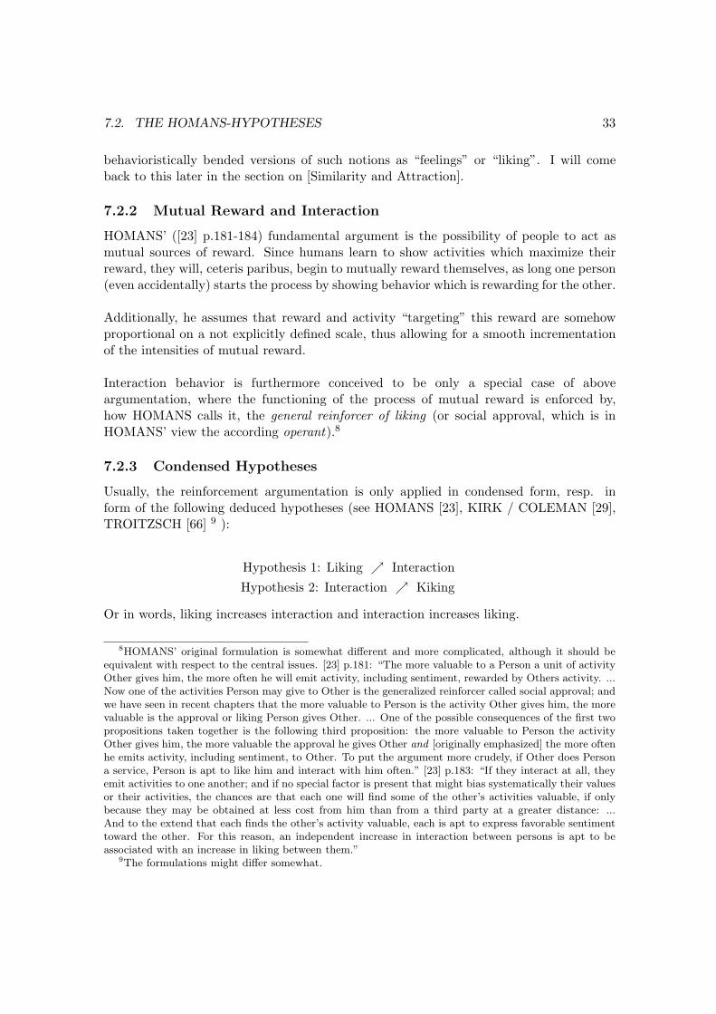
Usually, the reinforcement argumentation is only applied in condensed form, resp. inform of the following deduced hypotheses (see HOMANS [23], KIRK / COLEMAN [29],TROITZSCH [66] 9 ):
Hypothesis 1: Liking ↗ InteractionHypothesis 2: Interaction ↗ Kiking
Or in words, liking increases interaction and interaction increases liking.
8HOMANS’ original formulation is somewhat different and more complicated, although it should beequivalent with respect to the central issues. [23] p.181: “The more valuable to a Person a unit of activityOther gives him, the more often he will emit activity, including sentiment, rewarded by Others activity. ...Now one of the activities Person may give to Other is the generalized reinforcer called social approval; andwe have seen in recent chapters that the more valuable to Person is the activity Other gives him, the morevaluable is the approval or liking Person gives Other. ... One of the possible consequences of the first twopropositions taken together is the following third proposition: the more valuable to Person the activityOther gives him, the more valuable the approval he gives Other and [originally emphasized] the more oftenhe emits activity, including sentiment, to Other. To put the argument more crudely, if Other does Persona service, Person is apt to like him and interact with him often.” [23] p.183: “If they interact at all, theyemit activities to one another; and if no special factor is present that might bias systematically their valuesor their activities, the chances are that each one will find some of the other’s activities valuable, if onlybecause they may be obtained at less cost from him than from a third party at a greater distance: ...And to the extend that each finds the other’s activity valuable, each is apt to express favorable sentimenttoward the other. For this reason, an independent increase in interaction between persons is apt to beassociated with an increase in liking between them.”
9The formulations might differ somewhat.
34 CHAPTER 7. THE KIRK-COLEMAN-MODEL
These two hypotheses are the theoretical foundations of the various models invoked inthe article of KIRK and COLEMAN for the attempt to instantiate the Simmel-Hypothesis.
Finally, I should again emphasize the fact that these formulations abstract fromthe more fundamental hypothesized process. The condensed Homans-hypotheses are onlyprojections of iterative instantiation of the same hypothesis of reinforcement learning inthe involved individuals.
7.3 The Kirk-Coleman-Model
After having introduced scope and theoretical foundations, I will informally describe thestochastic simulation model.
As mentioned before, the Kirk-Coleman-Model is a microscopic simulation of theassumed process of interaction in a three person group. The program instructions 10
modelling the individual behavior are mapping the condensed versions of the Homans-Hypotheses as they are declared in the last section. A single turn of the simulationproceeds as follows (KIRK / COLEMAN [29]: pp. 176).
• Every Individual i = 1, 2, 3 chooses one of the other individuals as preferred inter-action partner. The probability of choosing an individual j is proportional to theliking for that individual.
• A single individual starts interaction with a probability proportional to a (at leastsemantically macroscopic) parameter of dominance. As a result, the choice needsnot to be necessarily reciprocal.
• The realized interaction is counted and its initiator is given a reward K with acertain probability RA. If the choice has been reciprocal, the interaction partner isgiven a reward K with a equal probability RA. If the partner has originally chosena different individual, he is given the reward K with a different probability RB.
• The reward K is added to i ’s liking for the individual j it has just interacted with.
• Finally, all sympathies are lowered by multiplication with a shrinkage-parameter,thus ensuring that recent interactions have an greater effect than those further inthe past.
This procedure is iterated until the desired number of interactions is reached. 11
10The original program has been written in FORTRAN, but only the control flow is available in thearticle.
11The maximal number of iterations calculated by KIRK and COLEMAN was 1000.
7.4. VARIOUS GROUP-INTERACTION MODELS 35
7.4 Various Group-Interaction Models
As mentioned, there exist several models which are implementing the Homans’ Hypothe-ses, three alone within the scope of the article of KIRK and COLEMAN (namely their twomodels and SIMON’s group-level model). A fourth model has recently been developedby TROITZSCH [66] [67], which extends the Kirk-Coleman-Model with respect to thenumber of agents12 considered.
It is interesting to observe how the models differ with respect to the constraintsimposed on them by the different calculi and possibly by techniques of software-engineering. The latter are constraining the image set of a model in a similar way acalculus would do, because both are pre-structuring the image-set of the possible models.
An indicator for this effect is the “dominance” parameter in the actual Kirk-Coleman-Model. It seems to result from the necessity of sequentialization of the modelled process.There seems to be no theoretical justification for the notion of dominance, since itis first a macroscopic concept defined on more than a single individual, and second,the microscopic differential equations model of KIRK and COLEMAN ([29]: pp.174)is lacking this parameter. This is not surprising, since all equations in a differentialequations system are solved simultaneously per definition.
Today sequentialization of simulation models is usually accomplished either by thesoftware employed (by an interpreter like MATLAB for instance) or by making auxiliaryassumptions in special program structures.13 In simulation studies it is unnecessary tomix the semantics of theoretical notions with technical assumptions as it is the case withthe mentioned parameter of dominance.
12By “agent” I will denote the model-representation of an actor.13So, every MABS has structures where the interactions of the agent-objects are related to each other,
i.e. are synchronized or a-synchronized. The common practice to assign “threads” to the agent-objectsand thus assign them own processes makes no exception: It just passes the task to the operating systemand to code hidden in the depth of the memory.

36 CHAPTER 7. THE KIRK-COLEMAN-MODEL
Chapter 8
Modification of theKirk-Coleman-Model
Originally, the bayesian network-implementation of the Kirk-Coleman-model had beenintended as a proof of the viability of the proposed method of level-transitory explana-tion. But when I started the actual modelling and tried to get rid of the semanticallymacroscopic parameter of dominance, I think I overshot by making the model “better”,i.e. more coherent and fashionable.
Since experience is the thing which one gets only after having needed it, the nowmodified model can not directly be compared with its original. Nevertheless, it still showsthe applicability of level-transitory explanation and resulted in interesting theoreticaldiscussion, which shall be demonstrated within this section.
8.1 Homans-Hypotheses and Expected Utility
Within this section I will argue that the Homans-hypotheses (as a special case ofreinforcement learning) along with the Subjective-Expected-Utility (SEU) hypothesiscan be interpreted as special cases of considerations regarding adaptation of systems toenvironmental conditions.
My interest in Expected Utility is driven by the fact that it is rather explicitlyformulated and widely welcomed in different disciplines.1
8.1.1 Subjective Expected Utility Theory
I will begin with a short sketch of subjective expected utility theory since the theory ofHOMANS is already introduced.
1I would certainly resist the temptation to dogmatically propose it as standard template for models ofhuman behavior.
37
38 CHAPTER 8. MODIFICATION OF THE KIRK-COLEMAN-MODEL
SEU has its foundations in the Theory of Games developed by VON NEUMANN/ MORGENSTERN [42], where maximization of the so called expectation function (orNeumann-Morgenstern-equation), which combines estimates of probability of events withestimates on the utility of these events, is shown to be the optimal guide for decisionsunder uncertainty.
These mathematical considerations were brought to a level of social science by SI-MON [58] who introduced the notion of bounded rationality, emphasizing the fact thatactual people do not act as desired by normative decision theory. A further milestonein the development of SEU-Theory were the studies of KAHNEMAN / TVERSKY[26] resulting in prospect theory which shows the cognitive biases in real-world decisionbehavior.
The subjective expected utility hypothesis can be formulated as follows:
Action =n∑
j=1
U(cj(ai))P (cj(ai)) → maxi! (8.1)
This means that the action ai is chosen which maximizes the sum of subjective utilities Udefined on its consequences cj , weighted by the subjective probability P of this consequencecj . In other words, the action is chosen which maximizes the average utility expected bythe acting individual.2
8.1.2 Adaptation
Now let me introduce adaptation as an argument which will allow me to compare thetheories of reinforcement learning and expected utility.
According to the [Encyclopedia Britannica], adaptation means “the process in whichan animal or plant becomes fitted to its environment”. Extrapolated to systems, thisdefinition will well serve my purposes, given I avoid the trap of biologism by introducingmodes of selection which are adequate to the nature of the process considered. A biolog-ical mode of selection is by no means necessary for the application of evolutionary theory.3.
Back to the concept of adaptation, it most importantly implies that there exists acertain criterion of optimality which should be approximated by a system while itsstate is disturbed by the environment (compare BISCHOF [5] on whom much of this
2Results of formulae of this structure are called “expectations” in probability theory. The notion of“expected utility” stems rather from this use of the word than from referring to subjective prospects, asused by KAHNEMAN / TVERSKY [26].
3Here an example: I can act in my shared flat in a variety of ways with every action having a certainpotential probability to be repeated in the presence of my flatmates. Thus one may say that there existsa certain fitness-function on my actions given my flatmates, ceteris paribus. But certainly my chances ofreproduction do not need to be mentioned if one analyzes this specific kind of evolutionary pressure. (Yet,my provocations have not been this extreme...)
8.1. HOMANS-HYPOTHESES AND EXPECTED UTILITY 39
argumentation is based). The existence of such a criterion of optimality is granted byevolutionary theory, for the reason that certain values of certain attributes may raise orlower a systems chance to exist in the future.
I will stop the considerations on evolution at this point since the question aboutevolutionary functionality of certain attributes is exactly the question about self-organization4 and functionality which I avoided in the [Emergence] section. It will fornow suffice to specify the criterion in the relevant context.
Returning to the question of modelling of individual level adaptation, I am nowable to state the following: A constructive hypothesis which models adaptive behaviormust necessarily combine elements representing assumptions on both
• on the optimal state of a system and
• the mechanism of its approximation given a particular environment.
8.1.3 Optimality and Reinforcement Learning
The behaviorist hypothesis of learning as invoked by HOMANS [22] [?] can be formulatedas follows:
A individual may be exposed to environmental stimuli as a result of showing aparticular behavior. These stimuli may either be experienced as rewarding or punishingby that individual. If the stimuli are experienced as rewarding, the probability ofoccurrence of the particular behavior will increase, which is called reinforcement. Ifthey are experienced as punishing, the probability will decrease, which is called extinction.
The proposal of representation of the optimal state is fulfilled (in this case implic-itly) by the notions of reward and punishment. Both can be understood as measuresof the gradient5 of the individual state which may be a complex function of individualbehavior and environment. If the individual is punished, it descents the gradient awayform the optimal state; if it is rewarded, it ascents the gradient toward the optimal state.
The mechanism of approximation is the rather explicitly formulated process of re-inforcement and extinction. It is easy to see that iteration of the process will drive theindividual to an area of its behavioral space where reward is maximized and punishmentis minimized, namely somewhere near the optimal state.6
4Whereby in the case of evolution the system level is the population level.5An rough but rather intuitive description of the mathematical notion of “gradient” could be the change
of a state with respect to all its defining attributes.6This procedure can be seen analogously to optimization by following the maximum gradient, together
with the associated problem of finding only local optima.
40 CHAPTER 8. MODIFICATION OF THE KIRK-COLEMAN-MODEL
8.1.4 Optimality and Expected Utility
The operation of subjective expected utility theory with regard to adaptation can beviewed analogously to the case of reinforcement learning. The difference between boththeories consists in the fact that in the case of SEU there is the additional assumption ofrepresentation of some features of the environment within the individual.
This representation of environment features is indirectly accomplished via the subjectiveprobability term of the SEU formula, since it states the feasibility of the respective actions.
Again, the optimal state is implicitly defined by a gradient-formulation, namelythose of utility. States of the environment (action consequences) with positive utilitypush the individual up the gradient of the “well-being function”, environmental stateswith negative utility push it down the gradient. Since the utilities are defined as beingsubjective estimates, they might be seen as “within-individual” representations, as well.
Given certain correspondence of the intra-individual representations with their real-worldtargets, iteratively maximizing the expected utility will finally result in approximatingthe optimal state.7
8.1.5 Evaluation of the Theories
In comparison with reinforcement learning, the representation of experience by a explicitset of subjective probabilities in SEU theory seems much more concise than summoninga vague “history of reinforcements”. Needless to say that today one is not bound to“scientific” formulation which omits latent variables and processes.
Summarized, SEU can be seen as the more explicit theory and shows more coher-ence to “common sense” than reinforcement learning, besides the fact that is well testedempirically. Therefore I decided to replace the Homans-Hypotheses by a SEU formulationin my model, interpreting liking as a subjective assessment of utility and defining theaction to be considered as the choice of an interaction-partner.8
But nevertheless, the relative simplicity of the behaviorist approach (including HOMANS’[Condensed Hypotheses]) is astonishing. Looking back, I would decide for the originalHomans-hypotheses if I had to do the project again, for the sake of comparability andsimplicity.
7It should make no sense to exaggerate the argument and talk about the “evolutionary advantage” ofrepresentation of the environment. Such a discussion would make it necessary to model the actual systemin which evolution takes place.
8Certainly the decision was supported by important social factors: I wanted to do something modern.And furthermore it pleased the sociologists and social-psychologists I am working with.
8.2. SIMILARITY AND ATTRACTION 41
8.2 Similarity and Attraction
By referring to “emission of feelings” [23]: p.181) or by invoking liking as “activity”,namely the “reinforcer called social approval” [23]: p.181), HOMANS clearly highlightsthe limitations of methodological behaviorism. The formulations are very clumsy andcontradictory to common sense, obviously in order to satisfy the demands of an obsoletetheory of knowledge. Luckily, neither KIRK and COLEMAN [29] nor TROITZSCH [66],[67] are continuing these definitory acrobatics.
In order to bypass these problems and have a definition of liking which is bothpsychologically sound and ready for easy operationalization, I employed BYRNE’s [8]theory of attitude- similarity. In essence, BYRNE proposes that attitude-similarity isthe main determinant of interpersonal attraction, with the relationship between the twovariables being linear positive. According to BAMBERG9, this proposition has beenconfirmed in numerous studies.
In effect, I employed the notion of attitude-similarity as a proxy for liking since Idid not incorporate factors to the model which could interfere with their relationship.
8.3 Feedback
In the original model of KIRK and COLEMAN the feedback-relation between liking andinteraction is realized by proposing two counterdirected effects connecting these variables(see [Condensed Hypotheses]). The implementation proceeds analogously with explicitrepresentation of the hypotheses (compare section [The Kirk-Coleman-Model]).
Now for the case of SEU-theory, the introduction of feedback to the process couldhave been accomplished as it is done implicitly by HOMANS’ reinforcement argumen-tation. There he proposes that the change of attractivity is a function of the kind ofbehavior, assumed that the individuals can interact in more than one way.10 This resultsin mutual dependency of liking and interaction. Thus, feedback might to be said animplicit attribute of the setup of the system of interaction, regardless of the kind ofadaptation-hypothesis employed.
Needless to say that I discovered this fact after already having implemented themodel. For sake of my reputation I have to emphasize that this account on feedback getslost in the projection from theory towards the [Condensed Hypotheses].
As a consequence, I modelled the feedback-process with the introduction of Social
9The information was given to me during a personal conversation. SEBASTIAN BAMBERG is a seniorlecturer of Social Psychology at the University of Giessen.
10This can be shown by the following passage: “...that every person evaluates some of the activities ofthe others as valuable...” (“...dass jede Person einige Aktiviteaten der anderen Person wertvoll findet...”[?]: p.155).
42 CHAPTER 8. MODIFICATION OF THE KIRK-COLEMAN-MODEL
Impact Theory, which replaced in alliance with SEU the two original hypotheses of theKirk-Coleman-model.
8.3.1 Social Impact Theory
LATANE’s [32] Social Impact Theory (SIT) is a rather concise theory determining theimpact of social influence on individual action and behavior. It is defined by the followingtwo equations. The first formulates the “principle of social forces”.
Imp = f(SIN) (8.2)
Where the social impact Imp is defined as a multiplicative function f of the strength S,the immediacy I and the number N of sources of social influence.
The second equation formulates the “psychosocial law”:
Imp = sN t | 0 < t < 1 (8.3)
Where the social impact Imp is defined by a power function of the number N of sourcesof social influence. Here s plays the role of a scaling constant, while the exponent t isrequired to be in the interval of (0 : 1).
The equation has the following properties: it increases monotonous while its derivativedecreases monotonous, which results in decreasing marginal impact.11 Furthermore, if theexponent t converges to 0, the function will approximate a constant function while it willapproximate a linear function if t converges to 1.
The name “psychosocial law” derives from the “psychophysical law” of STEVENS,which employs the same formulation to relate objective and experienced intensity ofstimuli.
Social Impact Theory can be evaluated as a simple and well established phenomenologicalaccount on social influence. (compare TANFORD / PENROSE [64]).
8.4 Agent Level Theory: Action and Social Influence
The integration of both Subjective Expected Utility and Social Impact Theory is accom-plished by invoking the previously introduced considerations on employment of attitude-similarity as a proxy for liking, resp. utility. This allows for attitudes being the basis fordecisions on interaction and then being interaction being the basis for changes in attitudes:
SEU: Attitude-Similarity → Interaction11This means that the more sources of influence are present, the less difference makes the appearance of
a additional source.

8.4. AGENT LEVEL THEORY: ACTION AND SOCIAL INFLUENCE 43
SIT: Interaction → Attitude-Similarity
This is the general theoretical setup of the Modified Kirk-Coleman-Model on thepsychological- resp. agent-level.

44 CHAPTER 8. MODIFICATION OF THE KIRK-COLEMAN-MODEL
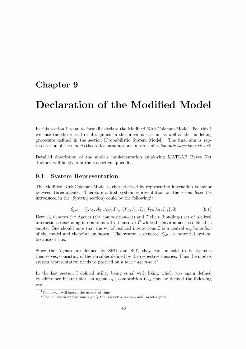
Chapter 9
Declaration of the Modified Model
In this section I want to formally declare the Modified Kirk-Coleman-Model. For this Iwill use the theoretical results gained in the previous section, as well as the modellingprocedure defined in the section [Probabilistic System Model]. The final aim is rep-resentation of the models theoretical assumptions in terms of a dynamic bayesian network.
Detailed description of the models implementation employing MATLAB Bayes NetToolbox will be given in the respective appendix.
9.1 System Representation
The Modified Kirk-Coleman-Model is characterized by representing interaction behaviorbetween three agents. Therefore a first system representation on the social level (asintroduced in the [System] section) could be the following1:
Spot = 〈{A1,A2,A3}, I ⊆ {I12, I13, I21, I23, I31, I32}, ∅〉 (9.1)
Here Ai denotes the Agents (the composition-set) and I their (bonding-) set of realizedinteractions (excluding interactions with themselves)2 while the environment is defined asempty. One should note that the set of realized interactions I is a central explanandumof the model and therefore unknown. The system is denoted Spot , a potential system,because of this.
Since the Agents are defined by SEU and SIT, they can be said to be systemsthemselves, consisting of the variables defined by the respective theories. Thus the modelssystem representation needs to proceed on a lower agent-level.
In the last section I defined utility being equal with liking which was again definedby difference in attitudes, an agent Ai’s composition CAi may be defined the followingway:
1For now, I will ignore the aspect of time.2The indices of interactions signify the respective source- and target-agents.
45
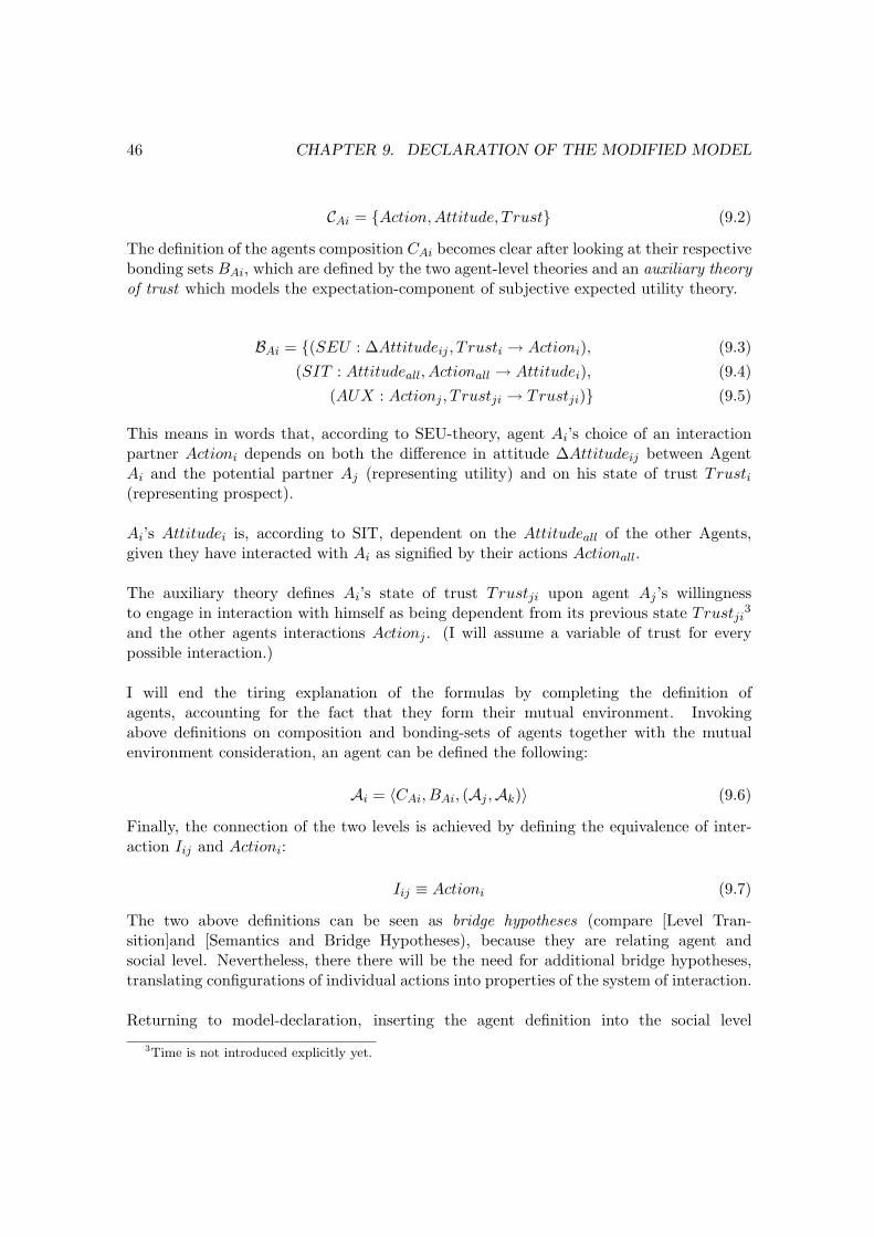
46 CHAPTER 9. DECLARATION OF THE MODIFIED MODEL
CAi = {Action,Attitude, Trust} (9.2)
The definition of the agents composition CAi becomes clear after looking at their respectivebonding sets BAi, which are defined by the two agent-level theories and an auxiliary theoryof trust which models the expectation-component of subjective expected utility theory.
BAi = {(SEU : ∆Attitudeij , T rusti → Actioni), (9.3)(SIT : Attitudeall, Actionall → Attitudei), (9.4)
(AUX : Actionj , T rustji → Trustji)} (9.5)
This means in words that, according to SEU-theory, agent Ai’s choice of an interactionpartner Actioni depends on both the difference in attitude ∆Attitudeij between AgentAi and the potential partner Aj (representing utility) and on his state of trust Trusti(representing prospect).
Ai’s Attitudei is, according to SIT, dependent on the Attitudeall of the other Agents,given they have interacted with Ai as signified by their actions Actionall.
The auxiliary theory defines Ai’s state of trust Trustji upon agent Aj ’s willingnessto engage in interaction with himself as being dependent from its previous state Trustji
3
and the other agents interactions Actionj . (I will assume a variable of trust for everypossible interaction.)
I will end the tiring explanation of the formulas by completing the definition ofagents, accounting for the fact that they form their mutual environment. Invokingabove definitions on composition and bonding-sets of agents together with the mutualenvironment consideration, an agent can be defined the following:
Ai = 〈CAi, BAi, (Aj ,Ak)〉 (9.6)
Finally, the connection of the two levels is achieved by defining the equivalence of inter-action Iij and Actioni:
Iij ≡ Actioni (9.7)
The two above definitions can be seen as bridge hypotheses (compare [Level Tran-sition]and [Semantics and Bridge Hypotheses), because they are relating agent andsocial level. Nevertheless, there there will be the need for additional bridge hypotheses,translating configurations of individual actions into properties of the system of interaction.
Returning to model-declaration, inserting the agent definition into the social level
3Time is not introduced explicitly yet.

9.2. TRANSITION GRAPH 47
composition, given by the first term of equation (33), completes the definition of themodels qualitative system representation:
S = 〈〈CA1, BA1, (A2,A3)〉, 〈CA2, BA2, (A1,A3)〉, 〈CA3, BA3, (A1,A2)〉〉 (9.8)
As we can see, the system exposes an obviously different structure on agent-level than onsocial level, namely because interactions are not explicitly specified as bonding relationsbut as components of the agents.4 However, I will soon restore proper social levelrepresentation.
Since equation (39) contains all bonding relations on the lowest level of definition,it constrains the system in a way that allows for deduction of interactions, given specificfunctional definitions and starting values.
In conclusion: Specific instances of S allow for deduction of actual realizations ofthe potential system Spot on social level.
9.2 Transition Graph
I will proceed by defining the transition representation of the Modified Kirk-Coleman-Model (see [Unfolding and Transition Representation]) and thus introduce time into themodel.
Sts(t,t+1) = 〈Cts(t,t+1), Ets(t,t+1),Bts(t,t+1)〉 (9.9)
Its familiar look (as compared to equation (40)) is restored by separating composition andbonding sets.
Cts(t,t+1) = {CA1t, CA2t, CA3t, CA1t+1, CA2t+1, CA3t+1} (9.10)
Bts(t,t+1) = {BA1unfolded, BA2unfolded, BA2unfolded} (9.11)
Ets(t,t+1) = {∅} (9.12)
In transition representation Sts(t,t+1), the composition set is “duplicated” (as long it doesnot change), in order to represent the objects in time explicitly. The unfolded bondingsets now contain relations between the objects which originate in the domain of t and endin t + 1.
4One should furthermore note that the environment E of the system S is still empty, regardless ofthe property that the agents form their mutual environment: The list of remaining agents A within theparticular agent (CAi, BAi, (Aj ,Ak)) can be interpreted as recursive pointer to their respective definitions.In fact, this represents properties of the bonding set, not the environment set.
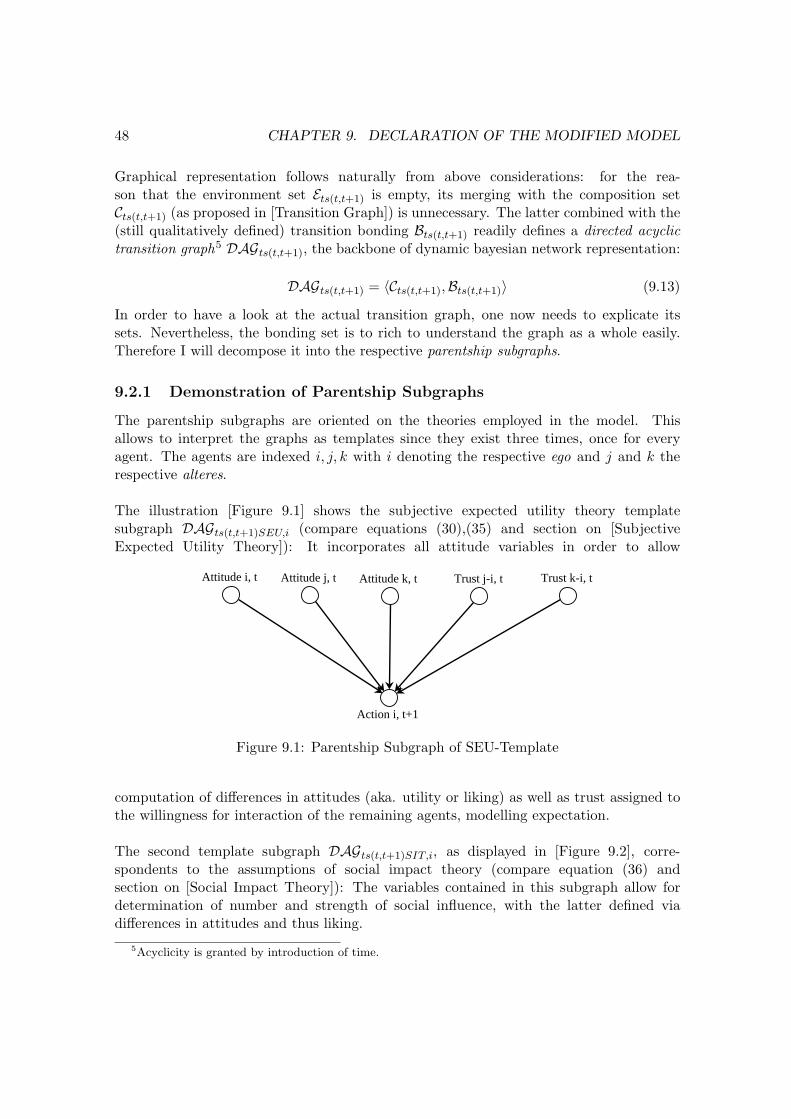
48 CHAPTER 9. DECLARATION OF THE MODIFIED MODEL
Graphical representation follows naturally from above considerations: for the rea-son that the environment set Ets(t,t+1) is empty, its merging with the composition setCts(t,t+1) (as proposed in [Transition Graph]) is unnecessary. The latter combined with the(still qualitatively defined) transition bonding Bts(t,t+1) readily defines a directed acyclictransition graph5 DAGts(t,t+1), the backbone of dynamic bayesian network representation:
DAGts(t,t+1) = 〈Cts(t,t+1),Bts(t,t+1)〉 (9.13)
In order to have a look at the actual transition graph, one now needs to explicate itssets. Nevertheless, the bonding set is to rich to understand the graph as a whole easily.Therefore I will decompose it into the respective parentship subgraphs.
9.2.1 Demonstration of Parentship Subgraphs
The parentship subgraphs are oriented on the theories employed in the model. Thisallows to interpret the graphs as templates since they exist three times, once for everyagent. The agents are indexed i, j, k with i denoting the respective ego and j and k therespective alteres.
The illustration [Figure 9.1] shows the subjective expected utility theory templatesubgraph DAGts(t,t+1)SEU,i (compare equations (30),(35) and section on [SubjectiveExpected Utility Theory]): It incorporates all attitude variables in order to allow
Attitude i, t Attitude j, t Attitude k, t Trust j-i, t Trust k-i, t
Action i, t+1
Figure 9.1: Parentship Subgraph of SEU-Template
computation of differences in attitudes (aka. utility or liking) as well as trust assigned tothe willingness for interaction of the remaining agents, modelling expectation.
The second template subgraph DAGts(t,t+1)SIT,i, as displayed in [Figure 9.2], corre-spondents to the assumptions of social impact theory (compare equation (36) andsection on [Social Impact Theory]): The variables contained in this subgraph allow fordetermination of number and strength of social influence, with the latter defined viadifferences in attitudes and thus liking.
5Acyclicity is granted by introduction of time.
9.2. TRANSITION GRAPH 49
Attitude i, t Attitude j, t Attitude k, t Action j, t Action k, t
Attitude i, t+1
Figure 9.2: Parentship Subgraph of SIT-Template
The last template subgraph DAGts(t,t+1)TRU,i is the one assigned to the auxiliarytheory of trust (compare equation (37)), which is displayed in [Figure 9.3] and will soonbe explained in detail: This subgraph expresses the dependency of current trust on
Action j, t Trust j-i, t
Trust j-i, t+1
Figure 9.3: Parentship Subgraph of Trust-Template
previous trust and action of the trusted.
As stated, the transition graph DAGts(t,t+1) is the union of the template subgraphs forall agents.
DAGts(t,t+1)A,i = DAGts(t,t+1)SEU,i ∪ DAGts(t,t+1)SIT,i ∪ DAGts(t,t+1)TRU,i (9.14)
DAGts(t,t+1) = DAGts(t,t+1)A,1 ∪ DAGts(t,t+1)A,2 ∪ DAGts(t,t+1)A,3 (9.15)
Equation (46) shows the aggregation of an individual agent transition subgraph from thetheoretic template subgraphs, while equation (47) shows the aggregation of the systemstransition graph from the individual agent subgraphs.
Finally, with [Figure 9.4], I also provide an illustration on the complete transitiongraph DAGts(t,t+1) which might look a little complicated compared to the previous
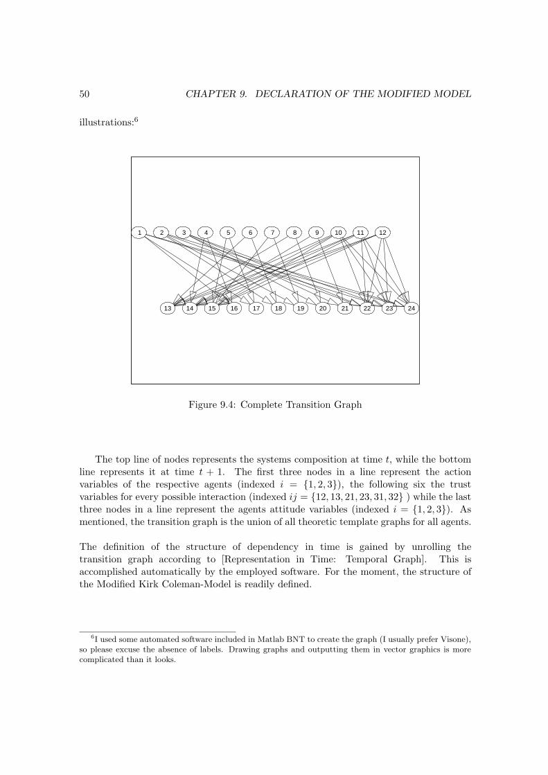
50 CHAPTER 9. DECLARATION OF THE MODIFIED MODEL
illustrations:6
1 2 3 4 5 6 7 8 9 10 11 12
13 14 15 16 17 18 19 20 21 22 23 24
Figure 9.4: Complete Transition Graph
The top line of nodes represents the systems composition at time t, while the bottomline represents it at time t + 1. The first three nodes in a line represent the actionvariables of the respective agents (indexed i = {1, 2, 3}), the following six the trustvariables for every possible interaction (indexed ij = {12, 13, 21, 23, 31, 32} ) while the lastthree nodes in a line represent the agents attitude variables (indexed i = {1, 2, 3}). Asmentioned, the transition graph is the union of all theoretic template graphs for all agents.
The definition of the structure of dependency in time is gained by unrolling thetransition graph according to [Representation in Time: Temporal Graph]. This isaccomplished automatically by the employed software. For the moment, the structure ofthe Modified Kirk Coleman-Model is readily defined.
6I used some automated software included in Matlab BNT to create the graph (I usually prefer Visone),so please excuse the absence of labels. Drawing graphs and outputting them in vector graphics is morecomplicated than it looks.
9.3. FUNCTIONAL DEPENDENCIES: CONDITIONAL PROBABILITY TABLES 51
9.3 Functional Dependencies: Conditional Probability Ta-bles
What still lacks in order to complete the model-declaration is the definition of thefunctional dependencies defined on the nodes of the transition graph. In other words: theformal implementation of the theories constituting the bonding set, as stated in section[System Representation], needs to be accomplished.
As introduced in [A Sketch of Bayesian Networks], I will use the bayesian networkformalism for this. In order to achieve a bayesian network representation, the the alreadydefined transition graph needs to be backed up with conditional probability functionsrepresenting the mentioned theoretic assumptions. Since those theories are defined on adomain represented by the template transition subgraphs introduced in the last section,I will attach the conditional probability functions on them.
Intended for my own convenience, I assumed discrete variables and thus tables asconditional probability functions.7. The tables are defined on variables with the followingdomains:
Actioni ∈ {1, 2} (9.16)Attitudei ∈ {1, 2, 3, 4, 5, 6, 7} (9.17)
Trusti ∈ {1, 2, 3, 4} (9.18)
The selection of domains is somewhat arbitrary, besides the proposal that the two lattershould represent ordinal information. Attitude is represented by seven values since this isa usual size of Likert-attitude scales.
In the following section I will discuss the constraints laid on those conditional proba-bility tables (CPD’s) by the model-formulations of the respective theories.
9.3.1 Subjective Expected Utility Theory
As can be seen in the first illustration in [Demonstration of Parentship Subgraphs] andequation (35), the structure of probabilistic formulation of the subjective expected utilityassumption within the modified Kirk-Coleman-model is the following:
P (Actioni,t+1) =
P (Actioni,t+1|Attitudei,t, Attitudej,t, Attitudek,t, T rustji,t, T rustki,t) (9.19)
Formulation of agent i’s utility Uij of interaction with agent j is given by the followingequation:
7It was intended for my convenience, but the decision did not pay out. Now I have got firmer knowledgeregarding modelling with theoretical probability distributions and clearly see the work and complicatednessI could easily have avoided. More on this later.
52 CHAPTER 9. DECLARATION OF THE MODIFIED MODEL
Uij =56
+16(1− |Attitudei −Attitudej |) (9.20)
This equation yields a definition of utility as being linearly decreasing with difference inattitudes and being normalized to the interval (1 : 0) for the defined domain of Attitude.Equality in attitudes results in an utility of 1 and maximum difference in an utility of 0.
Expected utility EU ij of the interaction is given by multiplication of utility Uij
with the respective value of trust Trustji in j’s willingness to return the favor ofinteraction:
EU ij = Uij Trustji (9.21)
This results in the possibility of an ordering of desirability of interaction choices.
Since deterministic maximization can not be modelled within an probabilistic framework,the agents are defined to choose interaction partners with a probability equal to theirrespective share of expected utility compared to the utility totally available at that time:
P (Actioni,t+1 = j) =EU ij∑n
j=1 EU ij|i 6= j (9.22)
Applying equation (54) to every possible configuration of its exogenous variables yields thedesired conditional probability table attached to the SEU-template parentship subgraph.It should be mentioned that it is large, namely 5488*2 cells.
9.3.2 Social Impact Theory
The structure of probabilistic dependency of the implementation of social impact theory(as introduced in [Demonstration of Parentship Subgraphs] and equation (36)) is thefollowing:
P (Attitudei,t+1) =
P (Attitudei,t+1|Attitudei,t, Attitudej,t, Attitudek,t, Actionj,t, Actionk,t) (9.23)
The implementation of social impact theory is somewhat more complicated than of SEU-theory. First, social impact is divided into three classes of influence, representing thebehavioral alternatives of the agent: influence towards a more negative (smaller) attitudevalue SIneg, influence towards perpetuation of the current attitude value SIperp andfinally towards a more positive (bigger) attitude value SIpos. The particular impact forthe respective class m is calculated according to following formula:
SIm = Uagents∈m sN(m)r | 0 < r < 1 (9.24)
This equation defines social impact SIm for the classes via the power function definedon the number of agents in the respective class m, as proposed by the “psychosocial law”,
9.3. FUNCTIONAL DEPENDENCIES: CONDITIONAL PROBABILITY TABLES 53
weighted by the mean utility Uagents∈m of the agents in this class. The term s is a scalingconstant, while the exponent r is required to be in the interval of (0:1) (compare sectionon [Social Impact Theory]).
It should be noted that the power function is not defined directly on the numberof agents in the respective class nm, but rather on a function of this number:
N(m) = nm | m = neg ∩m = pos (9.25)N(m) = nm + 1 q | m = perp (9.26)
For the case of influence towards change of attitude, the number of agents in the respec-tive class enters the social influence equation (56), while for the case of perpetuationof attitude the number of agents in the class is incremented by one, accounting for theown attitude. The increment is furthermore multiplied by q, a factor representing theego-agents resistance towards social influence. The higher q gets, the more important isthe own attitude compared to the others.
The probability of obedience to a particular impact class P (OBAm) is given by itsproportion relative to the total amount of impact:
P (OBAm) =OBAm
OBAneg +OBAperp +OBApos(9.27)
Since a more positive or negative attitude may be defined on more than one attitude value,the mass of the probability of change P (OBAm) may be required to be spread over thosevalues. The assumption that the probability of attitude change is linearly decreasing withits size is expressed by the following equation:
P (Attitudei = x) = P (OBAm) (1− |x−marginm|∑Xo=1 |o−marginm|
) | x ∈ m (9.28)
The probability of showing a particular attitude-value x is defined by weighting theprobability of obedience to a certain class of impact P (OBAm) by the inverse of its shareof the total distances towards the outer margin value of the particular category.
9.3.3 Auxiliary Assumptions on Trust
The structure of probabilistic dependency of the assumptions on trust, as defined in equa-tion (37) and the last template subgraph in section [Demonstration of Parentship Sub-graphs], is the following:
P (Trustji,t+1) =
P (Trustji,t+1|Trustji,t, Actionj,t) (9.29)
The idea is simply that trust in ones willingness to interact is increased if an interactionoccurs, while it is lowered when there is no interaction. In order to achieve probabilistic

54 CHAPTER 9. DECLARATION OF THE MODIFIED MODEL
formulation I assume a certain probability p of erroneous change of the value of trust.Again I assume small deviances to be more probable than large ones:
P (Trustji = x) = (1− p) e−α |x−true| (9.30)
For application of the equation α needs to be determined. The following solutions werecalculated using MAPLE, accounting for the fact that probabilities must sum to one:
α = 1.60289 | true ∈ margin (9.31)α = 2.13678 | true /∈ margin (9.32)
There exist two different solutions for the cases that the true value is on the margin ofthe domain of Trust or not, resp. for a “sloped” and a “peaked” distribution.
Above equations result in a probability distribution of trust which assigns a proba-bility 1 − p to the true value while the probabilities of realizing a different value areexponentially8 decreasing with the size of this respective difference.
I should note that the implementations of the three theories share a common at-tribute, namely that events with zero probability are assigned a new probability, onlyslightly greater than zero. This way I tried to allow for all defined events to be possible.
This concludes the declaration of the Modified Kirk-Coleman-Model. Finally, it isfar more complicated than the original, which was not really intended.
8If you compare this approach to the similar problem occurring in the implementation of SIT, you mywonder why I used both linear and exponential approaches. The honest answer is that these are ad hocmodelling solutions. In this case I was not able do guarantee positive probabilities by a linear approach andthe
∑X
i=1pi = 1 constraint. Therefore I used an exponential equation, although Ockhams Razor would
have requested a linear one.
Chapter 10
Model Sensitivity
During this section I will give a description of the results of the model. Please excuseme if the interpretation of the results is not too detailed, I just wanted to show that myphilosophical convictions can be coded in a working method. This is, what the modifiedKirk-Coleman model does.
10.1 Employed Soft- and Hardware
The model has been implemented employing MURPHY’s [40] Bayes Net Toolbox forMATLAB. (BNT) BNT is a GPL licensed library of MATLAB functions for learning andinference in bayesian networks, while MATLAB is a very widespread software packagefor scientific and technical computing. I first experimented with readily compiled andcomfortable software like NETICA and GENIE, but these proved to be unhandy forimplementation of dynamic bayesian networks. On the other hand I did not want towrite my implementation from scratch in a general language like C++, so the use ofa sophisticated library in an interpreted language like MATLAB looked promising. Afurther advantage were its graphics features.
The calculations were executed on a computer with AMD Athlon XP-2500 proces-sor and 512MB RAM running Windows XP operating system. A monte carlo parameterstudy of the model, running 100 times 100 time-steps took approximately seven hours ofprocessor time.
This fact implies that it would have been a better choice to separate simulationand analysis of the model by means of probabilistic inference. This could have beenaccomplished by implementing the model employing standard multi agent basedmethodology and rather use bayesian networks on top of model -generated data.
55
56 CHAPTER 10. MODEL SENSITIVITY
10.2 Solving the Model
Because of the size of the model (12 times t variables) and its temporal structure1, theapplication of exact algorithms for inference in bayesian networks has shown as beinginfeasible. After some bad experiences I finally arrived at Likelihood Weighting as anappropriate algorithm. I will give an introduction to it after a short summary of the trials.
For the case of the very popular Junction Tree Algorithm the software crashed ata model size of t ≈ 20, exceeding an amount of 2GB central memory. Application of theso called Boyen-Koller-Algorithm, which is specially designed for approximate inferencein temporal models, resulted in out-of-memory crashes at t ≈ 60.
Experimentation with MATLAB BNT’s implementation of Gibbs- Sampling, a sim-ulation algorithm which is todays silver bullet for probabilistic inference (see GILKSet.al. [17]), yielded results for t > 100, but those were obviously flawed. The inferreddistributions showed a strange pattern of entropy, switching between deterministic anduniform.2
10.2.1 Stochastic Sampling
Likelihood Weighting proved itself as a feasible approach. Being a sampling algorithm, itavoids computation with the actual rules of probability calculus but rather simulates the“random-experiments” which are modelled by it. Thus the concept of Joint ProbabilityDistribution is not needed for computation, resulting in a minimal need for computermemory.
In order to introduce the algorithm I need to provide a glance at the commonproblems associated with stochastic sampling. I will start with the introduction ofthe most common method called Rejection Sampling (compare PRESS et.al. [48]).An example will demonstrate the procedure: If we want to sample a distribution sayP (X) with P (Xi = x1) = 0.2 and P (Xi = x2) = 0.8 we will employ a pseudo randomgenerator which produces uniformly distributed sample values si in the interval (0 : 1).If si is < 0.2 we will assign a realization of x1 to it, if si is > 0.2 we will say thatx2 has been realized. This procedure is repeated until the counts of the sample valuesapproximate the probability distribution P (X) with desired accuracy.
The problematic issue is now that if the probability of a particular value of thedistribution gets sufficiently small, we will have to wait a long time until a sample valuerealizes this value. And we will have to wait a accordingly longer in order to get a sufficient
1I will not discuss this problem here. The reader is referred to JENSEN’s [25] treatment of the topic.2A better software implementing Gibbs Sampling and other MCMC-algorithms is WinBUGS. Its de-
signed for bayesian inference in graphical models, a method which extends this treatment of bayesiannetworks by the incorporation of knowledge known prior to data. Unfortunately, I discovered this softwareonly after having finished my computations on the modified Kirk-Coleman-model.
10.3. MONTE-CARLO PARAMETER STUDY 57
number of samples realizing this particular value. For example, if P (Xi = xj) is 0.001 wewill have to expect to draw thousand samples in order to get a single realization xj and amillion samples to get thousand counts of this specific value. One would have producedthousand times more samples than we wanted to.
In bayesian networks this problem has special significance since a sampling sweepthrough the net requires repeated sampling from multiple conditional distributions. Thismeans that whole configurations of values of parent variables have to be hit by thesampler in order to allow for realization of a certain value of the child variable.
Now Likelihood Weighting is an approach to avoid the problem of improbabilitycaused by multiple and nested conditions, as coded in the graphical structure of themodel. The idea is not to wait until some improbable conditional sample is drawn,but instead to sample from an unconditional distribution and then weight the samplewith the probability of its conditions, resp its parent distributions. This allows forsignificantly accelerated computation. A short description of the algorithm can be foundat RIEDMILLER [49].
For completeness I should mention another, more powerful, approach, namely Markov-Chain-Monte-Carlo or MCMC, of which the mentioned Gibbs-Sampling is a specialcase: here a markov-chain is specified in a way that ensures that its stationary limitingdistribution is equivalent to the distribution one wants to sample. The power of themethod consists in the fact that no redundant samples are produced. It extends theadvantages of likelihood weighting by the possibility to cope with improbabilities which donot stem from the structure of the bayesian network. Needless to say MCMC incorporatesvery sophisticated mathematics. Introduction can be found in GILKS et al. [17].
10.3 Monte-Carlo Parameter Study
In order get a proper idea of the models behavior I undertook a monte carlo parameterstudy of the model. The following parameters were instantiated with uniform randomvalues:
• Initial values of the systems variables Ct;
• Individual agents social impact theory parameters {qi, ri} as previously introduced;
• Individual agents probabilities pi of erroneous change of the value of Trusti;
One hundred monte-carlo runs of the model over 100 time-steps3 were calculated withthe result that the model converged towards joint uniform distribution under all instanti-ated conditions. I will present some illustrations to clarify this result.
3The number of steps was this low due to the massive amount of computations needed. Since theprocess always converged within less than half of the steps this should not be considered as a problem.
58 CHAPTER 10. MODEL SENSITIVITY
10.3.1 Illustrations of the Monte-Carlo-Runs
Some introduction will be helpful for interpretation. The graphs show attributes of indi-vidual systems variables plotted against time. The first half of the plots shows the changeof the variables expectation µ(v) while the second half shows its change of entropy H(v).The latter can be interpreted as a measure of dispersion (besides the fact that it is oneof the cental theoretical notions of information theory). An entropy of 0 signifies no dis-persion at all, while a maximum value signifies uniform distribution. I abstained fromcalculating standardized measures since all distributions converge to uniform and thusmaximum entropy. The respective maximum values Hmax(v) are:
Hmax(Action) = 1Hmax(Trust) = 2
Hmax(Attitude) = 2.807
[Figures 10.1 and 10.2] show the dynamics of agent A1’s interaction choice Action1.
As can be seen, the expectation and entropy rapidly converge towards indifference4, resp.maximum entropy which are functions of uniform distribution.
The same is true for the agents attitudes and trusts, where expectations convergetowards indifference and entropies towards maximum. Subsequently, two exemplarycharacteristics of agent A1, namely Attitude1 ([Figures 10.3 and 10.4]) and Trust12
([Figures 10.5 and 10.6]) are displayed. Please note that I am only showing illustrationsfor the first of the three agents, because the remaining ones look indistinguishable fromthese. (Compare [Appendixes] for complete results.)
10.3.2 Cluster-Analysis of the Monte-Carlo-Runs
A k-means cluster-analysis performed on the complete set of variables and runs supportsthe conclusion of convergence towards joint uniform distribution. According to its resultsit does not make sense to assume a partitioning of model runs. This is implicated bythe low and rather constant characteristic of the Scree-plots of Mean-Silhouette- ([Figure10.7]) and Gain-in-R2-Values ([Figure 10.8]).
Silhouette-Values are coefficients in the range of (−1 : 1), where -1 signifies aprobably mistaken cluster-assignment of a single data entry (run). Accordingly, a valueof 0 signifies an assignment to more than one cluster and a value of 1 a probably correctassignment. Gain-in-R2 denotes the increase of explained variance over the data entriescompared to a (k-1)-cluster solution and is sometimes called Eta-coefficient (compareBACHER [2]).
4Actioni has a domain of 1, 2, where a higher value corresponds to an agent with a higher index. Thusan expectation of 1.5 implies indifference. Compare [Functional Dependencies: Conditional ProbabilityTables] .
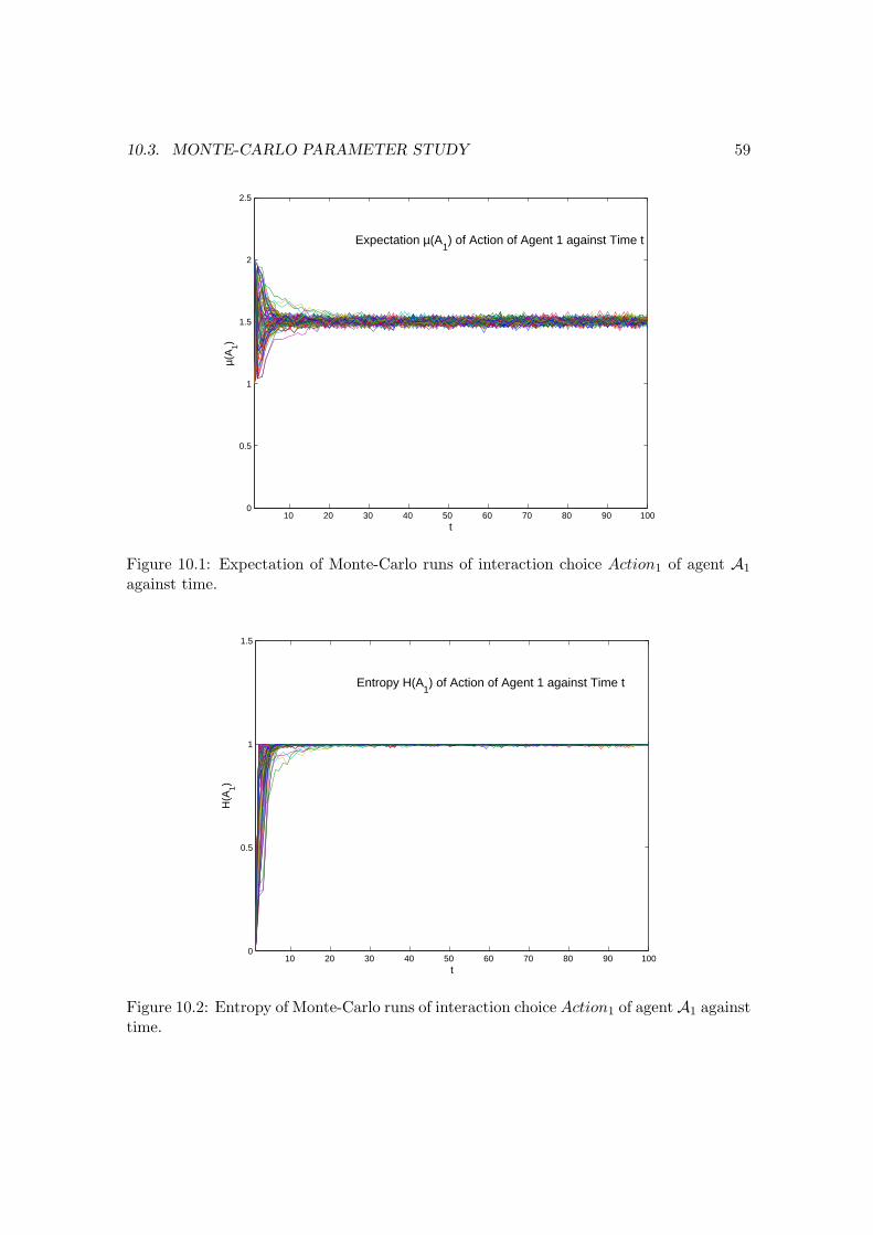
10.3. MONTE-CARLO PARAMETER STUDY 59
10 20 30 40 50 60 70 80 90 1000
0.5
1
1.5
2
2.5
t
µ(A
1)Expectation µ(A
1) of Action of Agent 1 against Time t
Figure 10.1: Expectation of Monte-Carlo runs of interaction choice Action1 of agent A1
against time.
10 20 30 40 50 60 70 80 90 1000
0.5
1
1.5
t
H(A
1)
Entropy H(A1) of Action of Agent 1 against Time t
Figure 10.2: Entropy of Monte-Carlo runs of interaction choice Action1 of agentA1 againsttime.
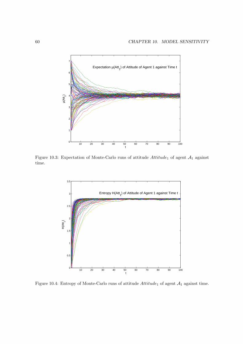
60 CHAPTER 10. MODEL SENSITIVITY
10 20 30 40 50 60 70 80 90 1000
1
2
3
4
5
6
7
t
µ(A
tt 1)Expectation µ(Att
1) of Attitude of Agent 1 against Time t
Figure 10.3: Expectation of Monte-Carlo runs of attitude Attitude1 of agent A1 againsttime.
10 20 30 40 50 60 70 80 90 1000
0.5
1
1.5
2
2.5
3
3.5
t
H(A
tt 1)
Entropy H(Att1) of Attitude of Agent 1 against Time t
Figure 10.4: Entropy of Monte-Carlo runs of attitude Attitude1 of agent A1 against time.
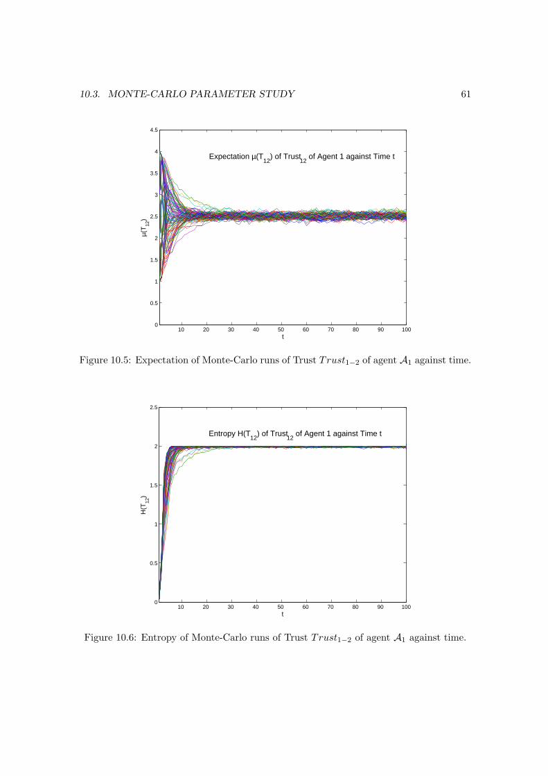
10.3. MONTE-CARLO PARAMETER STUDY 61
10 20 30 40 50 60 70 80 90 1000
0.5
1
1.5
2
2.5
3
3.5
4
4.5
t
µ(T
12)
Expectation µ(T12
) of Trust12
of Agent 1 against Time t
Figure 10.5: Expectation of Monte-Carlo runs of Trust Trust1−2 of agent A1 against time.
10 20 30 40 50 60 70 80 90 1000
0.5
1
1.5
2
2.5
t
H(T
12)
Entropy H(T12
) of Trust12
of Agent 1 against Time t
Figure 10.6: Entropy of Monte-Carlo runs of Trust Trust1−2 of agent A1 against time.
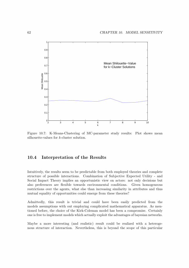
62 CHAPTER 10. MODEL SENSITIVITY
2 3 4 5 6 7 8 9 100
0.1
0.2
0.3
0.4
0.5
0.6
0.7
0.8
0.9
1
k
Mea
n S
hilo
uette
Mean Shilouette−Valuefor k−Cluster Solutions
Figure 10.7: K-Means-Clustering of MC-parameter study results: Plot shows meansilhouette-values for k-cluster solution.
10.4 Interpretation of the Results
Intuitively, the results seem to be predictable from both employed theories and completestructure of possible interactions. Combination of Subjective Expected Utility - andSocial Impact Theory implies an opportunistic view on actors: not only decisions butalso preferences are flexible towards environmental conditions. Given homogeneousrestrictions over the agents, what else than increasing similarity in attributes and thusmutual equality of opportunities could emerge from these theories?
Admittedly, this result is trivial and could have been easily predicted from themodels assumptions with out employing complicated mathematical apparatus. As men-tioned before, the choice of the Kirk-Coleman model has been a compromise. Certainlyone is free to implement models which actually exploit the advantages of bayesian networks.
Maybe a more interesting (and realistic) result could be realized with a heteroge-nous structure of interaction. Nevertheless, this is beyond the scope of this particular
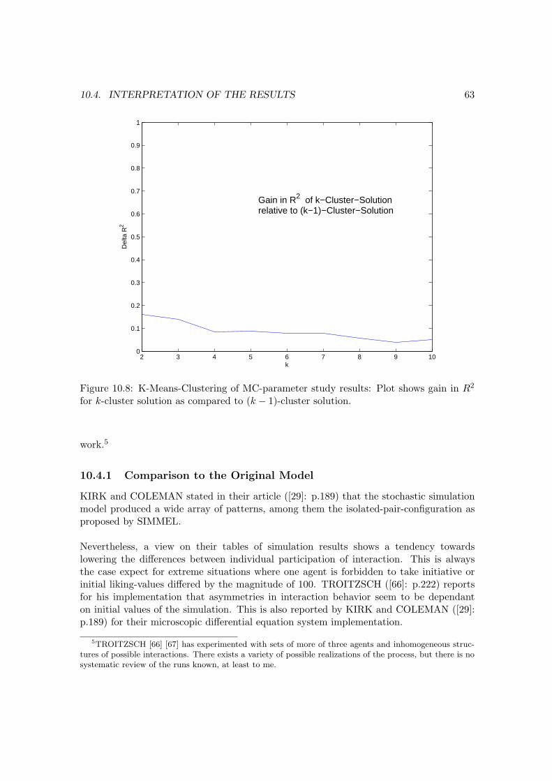
10.4. INTERPRETATION OF THE RESULTS 63
2 3 4 5 6 7 8 9 100
0.1
0.2
0.3
0.4
0.5
0.6
0.7
0.8
0.9
1
k
Del
ta R
2
Gain in R2 of k−Cluster−Solutionrelative to (k−1)−Cluster−Solution
Figure 10.8: K-Means-Clustering of MC-parameter study results: Plot shows gain in R2
for k-cluster solution as compared to (k − 1)-cluster solution.
work.5
10.4.1 Comparison to the Original Model
KIRK and COLEMAN stated in their article ([29]: p.189) that the stochastic simulationmodel produced a wide array of patterns, among them the isolated-pair-configuration asproposed by SIMMEL.
Nevertheless, a view on their tables of simulation results shows a tendency towardslowering the differences between individual participation of interaction. This is alwaysthe case expect for extreme situations where one agent is forbidden to take initiative orinitial liking-values differed by the magnitude of 100. TROITZSCH ([66]: p.222) reportsfor his implementation that asymmetries in interaction behavior seem to be dependanton initial values of the simulation. This is also reported by KIRK and COLEMAN ([29]:p.189) for their microscopic differential equation system implementation.
5TROITZSCH [66] [67] has experimented with sets of more of three agents and inhomogeneous struc-tures of possible interactions. There exists a variety of possible realizations of the process, but there is nosystematic review of the runs known, at least to me.

64 CHAPTER 10. MODEL SENSITIVITY
Sadly, KIRK and COLEMAN undertook no systematic parameter study and fur-thermore calculated maximally only 1000 iterations of the simulation. I assume that inthe case of the modified model convergence has been accelerated by the more powerfulfeedback mechanism of Social Impact Theory as compared to the “reward” of interactionin the original model. For the case of extreme initial conditions the SIT feedbackmechanism may have enabled convergence towards joint uniform distribution.
I finally arrived at the conclusion that the models behaviors do only differ withrespect to the strength of the feedback modifying agents preferences and that theSIMMEL-hypothesis cannot usually be realized by assumption of opportunistic actors,given homogeneous restrictions on their possible actions. Exceptional realization maybe enabled by initial conditions which exceed the impact of the particular feedbackmechanism on the agents preferences.
Chapter 11
Level-Transition Instantiated
As promised in the [Introduction] and the section [Level Transition], I will finally show animplementation of an actual level-transitory explanation in order to prove the feasibilityof both proposed methodology and method. Again, it should be understood rather as andemonstration than as a detailed analysis of the model.
In principle, the employed procedure (compare section on [Level Transition]) con-sists of the following operations:
• Definition of Bridge Hypotheses which translate properties on both levels;
• Performance of inference on the lower level: either exhausting the set of realizationsof higher level properties or sampling it;
• Aggregation of the results of lower-level inference over the functions defined by BridgeHypotheses, thus completing level transitory explanation;
This structure will organize the arrangement of the ongoing section. I will start by intro-ducing the theoretical circumstances of the example.
11.1 Bridge Hypothesis: Balance Theory Classification
Theoretical background of the example is HEIDER’s [19] Theory of Structural Balancewhich will deliver the bridge hypothesis to be considered. Balance Theory can be de-scribed as being similar to FESTINGER’s Theory of Cognitive Dissonance and analyzessocial situations with respect to the occurrence of dissonance. It should be mentionedthat Balance Theory is not connected to the employed agent level theories. Neverthelessit allows a good exemplification of the method. I will now briefly describe its basicassumptions.
65
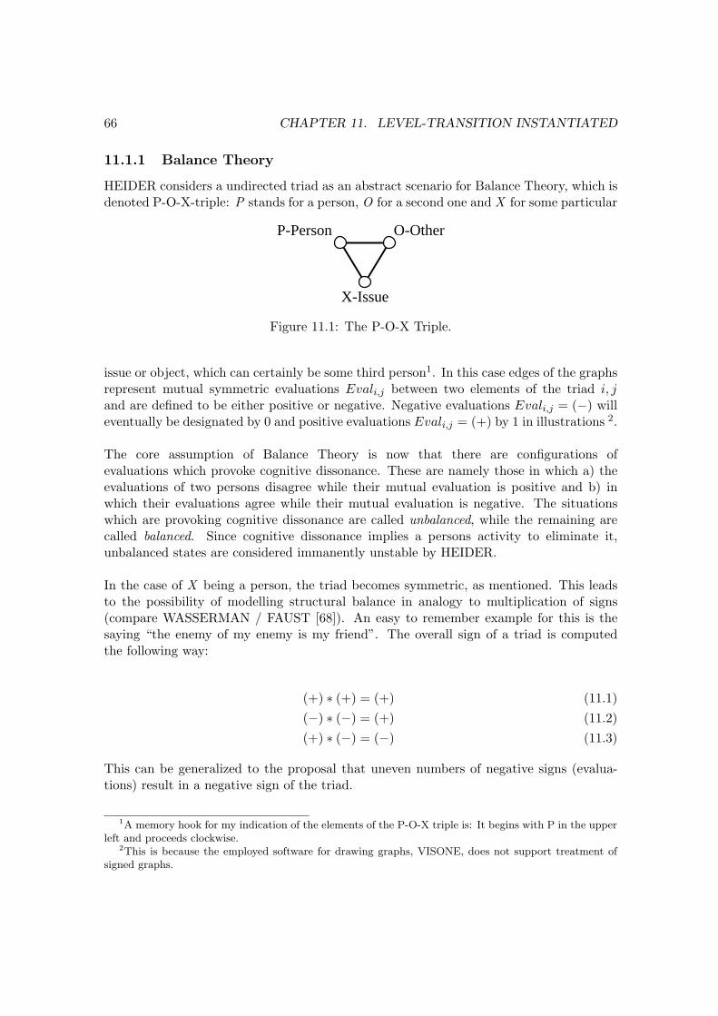
66 CHAPTER 11. LEVEL-TRANSITION INSTANTIATED
11.1.1 Balance Theory
HEIDER considers a undirected triad as an abstract scenario for Balance Theory, which isdenoted P-O-X-triple: P stands for a person, O for a second one and X for some particular
P-Person O-Other
X-Issue
Figure 11.1: The P-O-X Triple.
issue or object, which can certainly be some third person1. In this case edges of the graphsrepresent mutual symmetric evaluations Evali,j between two elements of the triad i, jand are defined to be either positive or negative. Negative evaluations Evali,j = (−) willeventually be designated by 0 and positive evaluations Evali,j = (+) by 1 in illustrations 2.
The core assumption of Balance Theory is now that there are configurations ofevaluations which provoke cognitive dissonance. These are namely those in which a) theevaluations of two persons disagree while their mutual evaluation is positive and b) inwhich their evaluations agree while their mutual evaluation is negative. The situationswhich are provoking cognitive dissonance are called unbalanced, while the remaining arecalled balanced. Since cognitive dissonance implies a persons activity to eliminate it,unbalanced states are considered immanently unstable by HEIDER.
In the case of X being a person, the triad becomes symmetric, as mentioned. This leadsto the possibility of modelling structural balance in analogy to multiplication of signs(compare WASSERMAN / FAUST [68]). An easy to remember example for this is thesaying “the enemy of my enemy is my friend”. The overall sign of a triad is computedthe following way:
(+) ∗ (+) = (+) (11.1)(−) ∗ (−) = (+) (11.2)(+) ∗ (−) = (−) (11.3)
This can be generalized to the proposal that uneven numbers of negative signs (evalua-tions) result in a negative sign of the triad.
1A memory hook for my indication of the elements of the P-O-X triple is: It begins with P in the upperleft and proceeds clockwise.
2This is because the employed software for drawing graphs, VISONE, does not support treatment ofsigned graphs.
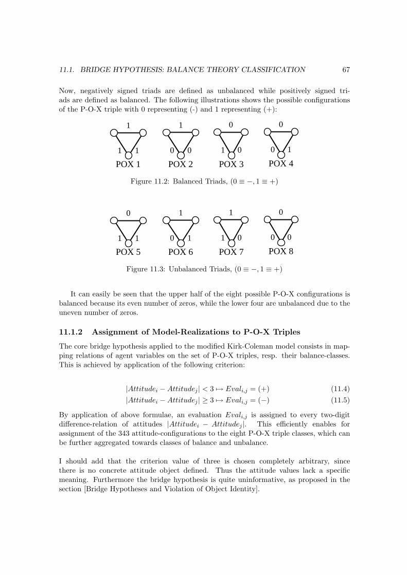
11.1. BRIDGE HYPOTHESIS: BALANCE THEORY CLASSIFICATION 67
Now, negatively signed triads are defined as unbalanced while positively signed tri-ads are defined as balanced. The following illustrations shows the possible configurationsof the P-O-X triple with 0 representing (-) and 1 representing (+):
1
1
1 0
1
0
0
1 0 0
0
1
POX 1 POX 2 POX 3 POX 4
Figure 11.2: Balanced Triads, (0 ≡ −, 1 ≡ +)
1
0
1 0
1
1
1
1 0 0
0
0
POX 5 POX 6 POX 7 POX 8
Figure 11.3: Unbalanced Triads, (0 ≡ −, 1 ≡ +)
It can easily be seen that the upper half of the eight possible P-O-X configurations isbalanced because its even number of zeros, while the lower four are unbalanced due to theuneven number of zeros.
11.1.2 Assignment of Model-Realizations to P-O-X Triples
The core bridge hypothesis applied to the modified Kirk-Coleman model consists in map-ping relations of agent variables on the set of P-O-X triples, resp. their balance-classes.This is achieved by application of the following criterion:
|Attitudei −Attitudej | < 3 7→ Evali,j = (+) (11.4)|Attitudei −Attitudej | ≥ 3 7→ Evali,j = (−) (11.5)
By application of above formulae, an evaluation Evali,j is assigned to every two-digitdifference-relation of attitudes |Attitudei − Attitudej |. This efficiently enables forassignment of the 343 attitude-configurations to the eight P-O-X triple classes, which canbe further aggregated towards classes of balance and unbalance.
I should add that the criterion value of three is chosen completely arbitrary, sincethere is no concrete attitude object defined. Thus the attitude values lack a specificmeaning. Furthermore the bridge hypothesis is quite uninformative, as proposed in thesection [Bridge Hypotheses and Violation of Object Identity].
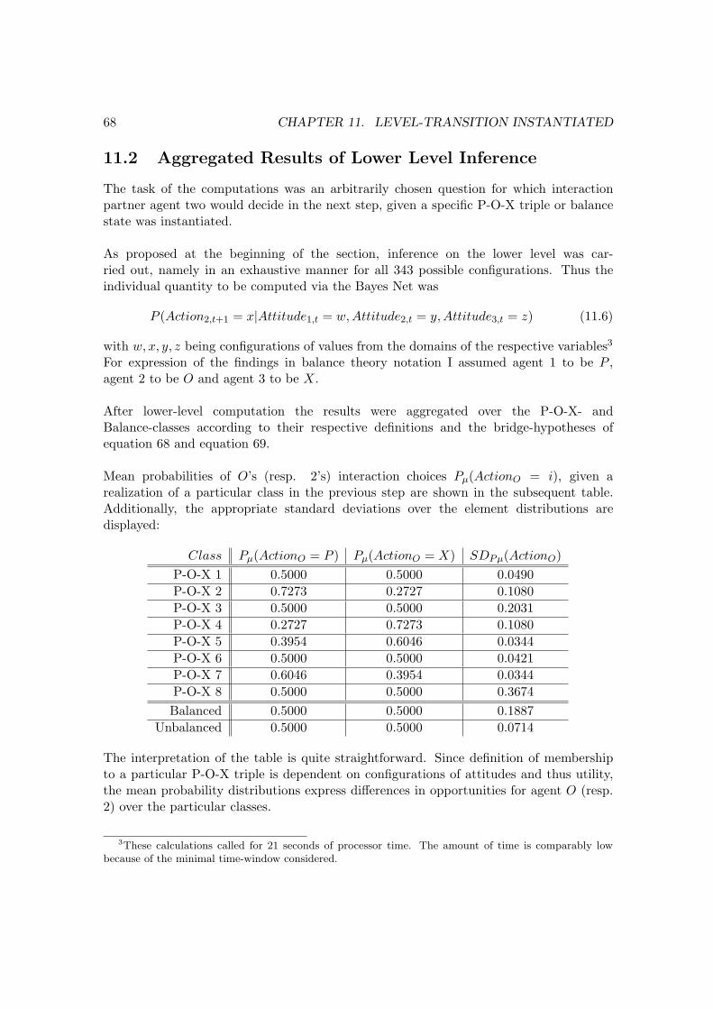
68 CHAPTER 11. LEVEL-TRANSITION INSTANTIATED
11.2 Aggregated Results of Lower Level Inference
The task of the computations was an arbitrarily chosen question for which interactionpartner agent two would decide in the next step, given a specific P-O-X triple or balancestate was instantiated.
As proposed at the beginning of the section, inference on the lower level was car-ried out, namely in an exhaustive manner for all 343 possible configurations. Thus theindividual quantity to be computed via the Bayes Net was
P (Action2,t+1 = x|Attitude1,t = w, Attitude2,t = y, Attitude3,t = z) (11.6)
with w, x, y, z being configurations of values from the domains of the respective variables3
For expression of the findings in balance theory notation I assumed agent 1 to be P ,agent 2 to be O and agent 3 to be X.
After lower-level computation the results were aggregated over the P-O-X- andBalance-classes according to their respective definitions and the bridge-hypotheses ofequation 68 and equation 69.
Mean probabilities of O’s (resp. 2’s) interaction choices Pµ(ActionO = i), given arealization of a particular class in the previous step are shown in the subsequent table.Additionally, the appropriate standard deviations over the element distributions aredisplayed:
Class Pµ(ActionO = P ) Pµ(ActionO = X) SDPµ(ActionO)P-O-X 1 0.5000 0.5000 0.0490P-O-X 2 0.7273 0.2727 0.1080P-O-X 3 0.5000 0.5000 0.2031P-O-X 4 0.2727 0.7273 0.1080P-O-X 5 0.3954 0.6046 0.0344P-O-X 6 0.5000 0.5000 0.0421P-O-X 7 0.6046 0.3954 0.0344P-O-X 8 0.5000 0.5000 0.3674Balanced 0.5000 0.5000 0.1887
Unbalanced 0.5000 0.5000 0.0714
The interpretation of the table is quite straightforward. Since definition of membershipto a particular P-O-X triple is dependent on configurations of attitudes and thus utility,the mean probability distributions express differences in opportunities for agent O (resp.2) over the particular classes.
3These calculations called for 21 seconds of processor time. The amount of time is comparably lowbecause of the minimal time-window considered.
11.2. AGGREGATED RESULTS OF LOWER LEVEL INFERENCE 69
In cases where the distribution is fifty/fifty the agents P and X are in averagesimply equally attractive. If a probability is greater than 0.5, this can be seen as a resultof asymmetric attractiveness corresponding to the definition of the respective P-O-Xtriple. A further indicator for this is the symmetry over the asymmetric distributionswithin a single balance-class: the probabilities are simply twisted (compare P-O-X2/P-O-X 4 and P-O-X 5/P-O-X 7, remembering that agent O is in the upper rightcorner). Differing probabilities over the triples of the two balance-classes are results ofthe asymmetric criterion value of three defined in equation 68 and equation 69.
Varying precision of aggregate predictions as given by the standard deviationsSDPµ(ActionO) cannot be so easily explained: detailed examination of the lowerlevel realizations should be necessary.
This should finish the treatment of the actual implementation of level transitoryexplanation. A description of impact of macroscopic states to individual action has beenachieved.
In the end, the actual process of computation might not seem too different fromwhat one would expect after being reminded of the Coleman-micro-macro scheme.Nevertheless, the problem consisted in proposing a method, which avoids mistakes. Andthere are truly enough opportunities for making mistakes with this particular question,especially at concept formation. The fact that the actual procedure seems trivial is agreat relief for me. The good ideas are always trivial with respect to something. Letshope that this is true for this work, too!

70 CHAPTER 11. LEVEL-TRANSITION INSTANTIATED
Chapter 12
Conclusion
At last I want to summarize the problems and solutions faced during the course of thiswork and furthermore give an outlook towards future research.
12.1 Summary: Problems and Solutions
The basic problem faced in an account on level-transitory explanation and thus emergenceis the identification of an appropriate criterion of object identity. This has been foundin the definition of objects by the set of causal mechanisms attached to these. Asbeing dependent on the conceivability of manipulation causality provides a criterionwhich assures object identity on all levels considered. Some might be disappointed bythis subjectivist approach, but I guess that proposition of restricted independence ofobject and observer is the only firm ground reachable during discussion of this matter.Furthermore the employed philosophical approach allowed for well founded criticism ofmethodology of both methodological individualism and bridge hypotheses.
For implementation of a proposed methodology of lower level inference, appropri-ate methods of computation were necessary in order to cope with complexity of systemstructures. Exemplary hazards of complexity are multicausality and nonlinearity ofinteractions. An appropriate method has been found with probability theory in itsformulation of bayesian networks: It allows for modelling of global processes by means ofstructures of local dependencies, while employing a mode of inference (marginalization,resp. integration) which is insensitive to the form of the actual functional dependencies.
The Kirk-Coleman-model proved to be a grateful toy for application of the methodologyand was modified in order to fit its requirements and include modern theories as SubjectiveExpected Utility and Social Impact Theory. Furthermore a method for translation ofSystem Representation into bayesian network Representation has been proposed.
Two types of calculations were undertaken with the modified Kirk-Coleman-model:First, a monte-carlo parameter study which led to the conclusion of convergence of the
71
72 CHAPTER 12. CONCLUSION
process towards joint uniform distribution under all instantiated conditions; and second,an actual realization of level-transitory explanation. A classification of states of the modelaccording to Balance-theory has been introduced and effects of macroscopic state-classeson a particular agent property (one time-step later in the model) have been computed.
Problematic issues concerning the modelling task were associated with the em-ployed algorithms and software. It turned out that even a “toy-application” like themodified Kirk-Coleman model easily puts bayesian networks inference algorithms totheir limits. Only sampling algorithms seemed to deliver appropriate performance. Dueto problems with the employed implementation of Gibbs-Sampling I finally used theLikelihood-Weighting algorithm. It turned out that application of standard simulationmethods for modelling combined with separate bayesian network analysis of generatedmodel data would have been a more practical approach. Reasons for this would be greaterease of implementation and enhanced speed of computation.
12.2 Outlook
There are some possible directions of future research which emanate from this work.
One direction would be to deepen its considerations regarding stability and emer-gence. I will track this path for personal interest, but the issue is complicated and has notyet revealed a promising starting point. What seems more promising is the applicationof the methodology to empirical problems. Either to structural analysis of rathersmall and completely surveyed social systems, or large scale data, utilizing structuralproxy-assumptions. The latter enterprise would certainly demand modified methodsof computation, like Synergetic or Bayesian Hierarchical Models , to name examples.Experimenting with this is in fact part of a plan about what to do this summer.

Acknowledgments
I have invested a lot time in considerations about the methodological foundations ofsocial theory, probably years if I start counting when the question first arose. Since a kindof result is achieved I will not complain about passed opportunities but instead engagein something tangible in my future. I have to thank many people, with no particular order:
My parents for supporting me and giving me the environment to grow mentally,my sister Birgit for being there and my brother Bruno, the smartest guy on the face ofearth, for being there to discuss issues over a long period of time.
My friends, especially Julia, Anna, Pierre, Martin, Guido and Thilo for cheeringme up and helping me to maintain my mental sanity. ;-) (And certainly you specifically!)
Peter Schmidt for giving me the opportunity to work on this topic and his con-stant encouragement to do things according to my own interests. Klaus Troitzsch forhis generous advice and steady support. Heinz Muehlenbein for showing me probabilitytheory and giving passionate criticism. Bernulf Kanitscheider for philosophical discussion.Eyke Huellermeyer for advice in matters of probability theory. Sebastian Bamberg fordiscussion of psychological issues. Krista Kinnius for counselling me with regard toEnglish language.
73

74 CHAPTER 12. CONCLUSION

Bibliography
[1] Alexander, Jeffrey C.; Giesen, Bernhard; Muench, Richard; Smelser, Neil J.; (Editors)“The Micro-Macro Link”; Berkeley 1987
[2] Bacher, Johann; “Clusteranalyse”; Muenchen 1994
[3] Baldi, Pierre; Brunak, Soeren; “Bioinformatics: the machine learning approach”;Massachusetts Institute of Technology 2001
[4] Bertalanffy, Ludwig von; “General System Theory: Foundation, Development, Appli-cations”; New York 1998
[5] Bischof, Norbert; “Struktur und Bedeutung: Eine Einfuehrung in die Systemtheorie”;Bern 1998
[6] Bunge, Mario; “Treatise on Basic Philosophy Vol. IV, Ontololgy II: A World of Sys-tems”; Dortrecht 1979
[7] Bunge, Mario; “Causality and Modern Science”; New York 1979
[8] Byrne, Donn; “The Attraction Paradigm”; New York 1971
[9] Carnap, Rudolf; “Grundlagen der Logik und Mathematik”; Muenchen 1973
[10] Churchland, Patricia S.; Sejnowski, Terrence J.; “The Computational Brain”; Cam-bridge, Massachusetts 1992
[11] Coleman, James S. ; “Introduction to Mathematical Sociology”; London 1964
[12] Coleman, James S. ; “Foundations of Social Theory”; Cambridge 1990
[13] Conte, Rosaria; Hegselmann, Rainer; Terna, Pietro; (Editors) “Simulating SocialPhenomena”; Berlin 1997
[14] Davidov, Eldad; Schmidt, Peter; “A Note: A Bridge between ’Bridge Assumptions’:Some Clarifications”; Unpublished Manuscript 2003
[15] Esser, Hartmut; “Die Definition der Situation”; in: Koelner Zeitschrift fuer Soziologieund Sozialpsychologie, Jg. 48, Heft 1, 1996, S.1-34
75
76 BIBLIOGRAPHY
[16] Gilbert, Nigel; Troitzsch, Klaus G.; “Simulation for the Social Scientist”; Bucking-ham 1999
[17] Gilks, W.R.; Richardson, S.; Spiegelhalter, D.J. (Editors); “Markov Chain MonteCarlo in Practice”; Boca Raton 1996
[18] Goerz, Guenther; Rollinger, Claus-Rainer; Schneeberger, Josef (Editors); “Handbuchder Kuenstlichen Intelligenz”; Muenchen 2003
[19] Heider, Fritz; “The Psychology of Interpersonal Relations”; New York 1958
[20] Heintz, Bettina; “Emergenz und Reduktion: Neue Perspektiven auf das Mikro-Makro-Problem”; in: Koelner Zeitschrift fuer Soziologie und Sozialpsychologie, Jg. 56, Heft1, 2004, S.1-31
[21] Holland, John; “Emergence: From Chaos to Order”; Reading, Massachusetts 1998
[22] Homans, George Caspar; “Theorie der sozialen Gruppe”; Opladen 1960
[23] Homans, George Caspar; “Social Behaviour: Its Elementary Forms”; London 1961
[24] Jaynes, Edwin T.; “Probability Theory with Applications in Science and En-gineering: A Series of Informal Lectures”; Fragmentary Edition of 1974,http://bayes.wustl.edu/etj/articles/mobil.pdf
[25] Jensen, Finn; “Introduction to Bayesian Networks und Decision Graphs”; Berlin/NewYork 2001
[26] Kahneman, Daniel; Tversky, Amos; “Prospect Theory: An Analysis of Decision underRisk”; Econometrica 47, Nr.2, 1979, p. 263 - 291
[27] Kelle, Udo; Luedemann, Christian; “Grau, teurer Freund, ist alle Theorie... Ratio-nal Choice und das Problem der Brueckenannahmen” in: Koelner Zeitschrift fuerSoziologie und Sozialpsychologie, Jg. 47, Heft 2, 1995, S.249-267
[28] Kelle, Udo; Luedemann, Christian; “Theoriereiche Brueckenannahmen? Eine Replikauf Siegwart Lindenberg” in: Koelner Zeitschrift fuer Soziologie und Sozialpsycholo-gie, Jg. 48, Heft 3, 1996, S.542-545
[29] Kirk, Jerome; Coleman, James; “Formalisierung und Simulation von Interaktionen ineiner Drei-Personen-Gruppe” in: Mayntz, Renate (Editor); “Formalisierte Modellein der Soziologie” Neuwied/Berlin 1967
[30] Lakatos, Imre; Musgrave, Alan; (Editors) “Criticism and the Growth of Knowledge”;Cambridge 1970
[31] Larson, Harold J.; “Introduction to Probability”; Reading, Massachusetts 1995
[32] Latane, Bibb; “The Psychology of Social Impact”; American Psychologist 36, 343-356
BIBLIOGRAPHY 77
[33] Lindenberg, Siegwart; “Die Relevanz Theoriereicher Brueckenannahmen”; in: Koel-ner Zeitschrift fuer Soziologie und Sozialpsychologie, Jg. 48, Heft 1, 1996, S.126-140
[34] Lindenberg, Siegwart; “Theoriegesteuerte Konkretisierung der Nutzentheorie; EineReplik auf Kelle/Luedemann und Opp/Friedrichs” ; in: Koelner Zeitschrift fuer Sozi-ologie und Sozialpsychologie, Jg. 48, Heft 3, 1996, S.560-565
[35] Luhmann, Niklas; “Soziale Systeme: Grundriss einer allgemeinen Theorie”; Frank-furt am Main 1996
[36] McClelland, David C.; “The Achieving Society”; New York 1967
[37] Mills, Theodore M.; “Soziologie der Gruppe”; Muenchen 1969
[38] Muehlenbein, Heinz; “Towards a Theory of Organisms and Evolving Automata: OpenProblems and Ways to Explore”; 2002
[39] Mueller-Benedict, Volker; “Selbstorganisation in Sozialen Systemen: Erkennung,Modelle und Beispiele nichtlinearer Dynamik”; Opladen 2000
[40] Murphy, Kevin; “Bayes Net Toolbox for Matlab” Documentation and Download at:http://www.ai.mit.edu/ murphyk/Software/BNT/bnt.html
[41] Nagel, Ernest; “The Structure of Science: Problems in the Logic of Scientific Expla-nation”; New York 1961
[42] Neumann, John von; Morgenstern, Oskar; “Theory of Games and Economic Behav-ior”; Princeton NJ 1953
[43] Nicholis, Gregoire; Prigogine, Ilya; “Die Erforschung des Komplexen”; Muenchen1987
[44] Opp, Karl-Dieter; “Methodologie der Sozialwissenschaften”; Wiesbaden 2002
[45] Opp, Karl-Dieter; Friedrichs, Juergen; “Brueckenannahmen, Produktionsfunktionenund die Messung von Praeferenzen”; in: Koelner Zeitschrift fuer Soziologie undSozialpsychologie, Jg. 48, Heft 3, 1996, S.546-559
[46] Pearl, Judea; “Probabilistic Reasoning in Intelligent Systems”; San Mateo CA 1988
[47] Pearl, Judea; “Causality”; Cambridge 2000
[48] Press, William H.; Flannery, Brian P.; Teukolsky, Saul A.; Vetterling, Wiliam T.;“Numerical Recipes in C: The Art of Scientific Computing”; Cambridge 1992
[49] Riedmiller, Martin; “Einfuehrung in die Kuenstliche Intelligenz. Veranstaltung 16:Inferenz in Bayes-Netzen”; Dortmund 2002,http://lrb.cs.uni-dortmund.de/ riedmill/teaching/ws0203 lect ki/ue16.pdf

78 BIBLIOGRAPHY
[50] Rohwer, Goetz; “Mehrebenenmodelle und das Mirko-Makro-Problem in der em-pirischen Sozialforschung”; 1998http://www.stat.ruhr-uni-bochum.de/papers.html
[51] Sawyer, R. Keith; “Nonreductive Individualism Part I - Supervenience and Wild Dis-junction” in: Philosophy of the Social Sciences Vol.32 No.4, Sage Publications, 2002,537-559
[52] Sawyer, R. Keith; “Nonreductive Individualism Part II - Social Causation” in: Phi-losophy of the Social Sciences Vol.33 No.2, Sage Publications, 2003, 203-224
[53] Scheibe, Erhard; “Die Reduktion physikalischer Theorien: Ein Beitrag zur Einheitder Physik”; Berlin 1997
[54] Schlick, Moritz; “Ueber den Begriff der Ganzheit” in: Topitsch(Edt.); “Logik derSozialwissenschaften”; Frankfurt am Main 1993
[55] Schnell, Rainer; Hill, Paul; Esser, Elke; “Methoden der Empirischen Sozialforschung”;Muenchen 1999
[56] Seiffert, Helmut; Radnitzky, Gerard; (Editors) “Handlexikon der Wissenschaftstheo-rie”; Muenchen 1992
[57] Simmel, Georg; “Soziologie: Untersuchungen ueber die Formen der Vergesellschaf-tung, Gesamtausgabe Band 11”; Frankfurt am Main 1999
[58] Simon, Herbert; “Bounded Rationality”; in: Simon, Herbert; “Models of BoundedRationality: Empirically Grounded Economic Reason Volume 3”, Massachusetts In-stitute of Technology 1997
[59] Simon, Herbert; “Simulation of Large Scale Systems by Aggregation”; in: Simon,Herbert; “Models of Bounded Rationality: Empirically Grounded Economic ReasonVolume 3”, Massachusetts Institute of Technology 1997
[60] Simon, Herbert; “The Architecture of Complexity: Hierarchic Systems”; in: Simon,Herbert; “Sciences of the Artificial”; Massachusetts Institute of Technology 1999
[61] Sosa, Ernest; Tooley, Michael; (Editors) “Causation”; Oxford 1993
[62] Stegmueller, Wolfgang; “Probleme und Resultate der Wissenschaftstheorie und Ana-lytischen Philosphie; Band I: Erklaerung, Begruendung, Kausalitaet; Teil E: Teleolo-gische Erklaerung, Funktionalanalyse und Selbstregulation. ...”; Berlin 1983
[63] Stegmueller, Wolfgang; “Probleme und Resultate der Wissenschaftstheorie und Ana-lytischen Philosphie; Band II: Theorie und Erfahrung; Teil F: Neuer Intuitiver Zu-gang zum strukturalistischen Theorienkonzept...”; Berlin 1986
[64] Tanford, Sarah.; Penrose, Steven.; “Social Influence Model: A Formal Integration ofResearch on Majority and Minority Influence Processes”; in: Psychological Bulletin95 1984

BIBLIOGRAPHY 79
[65] Troitzsch, Klaus G.; “Modellbildung und Simulation in den Sozialwissenschaften”;Opladen 1990
[66] Troitzsch, Klaus G.; “Individuelle Einstellungen und Kollektives Verhalten” in: Kuep-pers, Guenter (Editor); “Chaos und Ordnung: Formen der Selbstorganisation inNatur und Gesellschaft”; Stuttgart 1996
[67] Troitzsch, Klaus G.; “Dynamische Modelle komplexer sozialer Systeme: Was leis-ten Computersimulationen?” in: Mainzer, Klaus (Editor); “Komplexe Systeme undNichtlineare Dynamik in Natur und Gesellschaft”; Berlin 1999
[68] Wasserman, Stanley; Faust, Katherine; “Social Network Analysis: Methods and Ap-plications”; Cambridge 1994
[69] Weiss, Gerhard; (Editor) “Multiagent Systems”; Cambridge, Massachusetts 2000

80 BIBLIOGRAPHY

Appendix A
Online Provision
Appendixes can be accessed online at the following location:
http://www.stud.uni-giessen.de/ st1334/MicroMacro/append.html
The reason for online provision is to enable direct code-access.Since its amount adds up to 65 pages the reader might excuse its absence.
81

82 APPENDIX A. ONLINE PROVISION
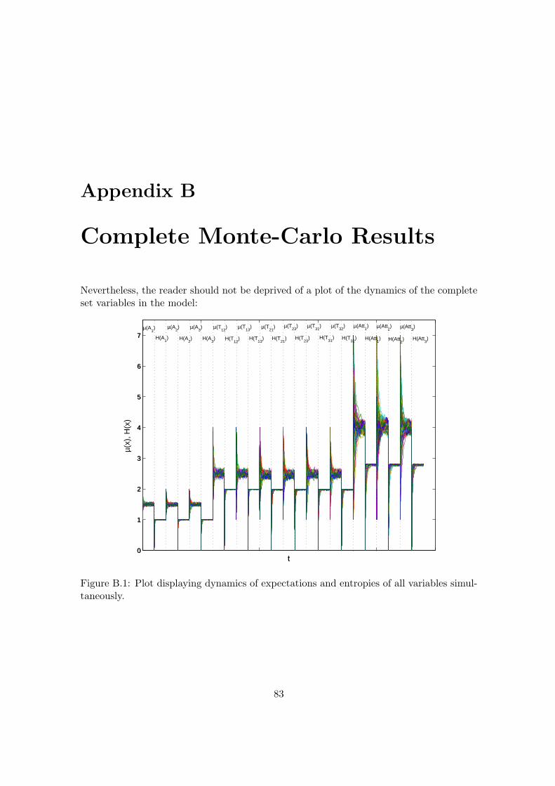
Appendix B
Complete Monte-Carlo Results
Nevertheless, the reader should not be deprived of a plot of the dynamics of the completeset variables in the model:
0
1
2
3
4
5
6
7
t
µ(x)
, H(x
)
0
1
2
3
4
5
6
7
t
µ(A1) µ(A
2) µ(A
3) µ(T
12) µ(T
13) µ(T
21) µ(T
23) µ(T
31) µ(T
32) µ(Att
1) µ(Att
2) µ(Att
3)
H(A1) H(A
2) H(A
3) H(Att
1) H(Att
2) H(Att
3) H(T
12) H(T
13) H(T
21) H(T
23) H(T
31) H(T
32)
Figure B.1: Plot displaying dynamics of expectations and entropies of all variables simul-taneously.
83