Micro-Fragmenting as a Method of Reef Restoration using · Micro-Fragmenting as a Method of Reef Restoration using Montipora capricornis Hannah Boyce MASSACHUSETTS ACADEMY OF MATH

Micro-Fragmenting

as a Method of Reef

Restoration using

Montipora

capricornis

Hannah Boyce MASSACHUSETTS ACADEMY OF MATH AND SCIENCE

M i c r o - F r a g m e n t i n g C o r a l | 1

Table of Contents

Abstract……………………………………………………………………………………………2

Introduction…………………………………………………………………………..……………3

Literature Review…………………………………………………….……………………………4

Research Plan…………………………………………………………………………………….25

Methodology…………………………………………………………………………………..…28

Results…………………………………………………………..………………………..………35

Data Analysis and Discussion……………………………………………………………………42

Conclusion……………………………………………………………...……………………...…44

Assumptions and Limitations……………………………………………………………….……45

Applications and Future Extensions……………………………………………………………...46

Literature Cited..………………………………………………………………………….………47

Appendix………………………………………………………………………………………….48

Acknowledgements……………………..………………………………………..…………….…51


Abstract

Micro-fragmenting is a process currently being used as a method of reef restoration for

coral reefs, but there have been few studies quantifying the effects of this process on growth rate.

The purpose of this project was to find the ideal size to micro-fragment coral. If one large piece

of Montipora capricornis is micro-fragmented into smaller pieces, ranging from 0-6 sq. cm

cross-sectional area, then the larger pieces will have a faster growth rate compared to the smaller

pieces. To perform this project, one piece of Montipora capricornis was cut, using a saw blade,

into 48 fragments. Each fragment was attached to ceramic disks using cyanoacrylate adhesive.

Fragments were placed in a 29-gallon tank equipped with lights, a filter, a heater, twelve

Calcinus spp. (red-legged hermit crabs), twelve Margarites pupillus (Margarita Snails), and live

rock. Supplements were added accordingly. The fragments were grown for nine weeks with

measurements taken approximately every two weeks. Exact measurements of fragments were

found using the computer imaging program, GIMP. There was a polynomial relationship

between the initial coral size and growth rate, with an r-squared value or 0.9219.


Introduction

While working with pieces of coral at MOTE Marine Laboratory in the Florida Keys,

David Vaughan accidently broke a piece of coral that had attached itself to the bottom of the

tank, and he thought nothing of this. A week later he came back to this tank and discovered that

this small piece of coral was not only still alive, but had also grown. He had discovered the

process of micro-fragmenting. Today MOTE Marine Laboratory uses the process of micro-

fragmenting to restore reefs, but there has not yet been any research that quantifies the difference

in growth rate between micro-fragmented pieces of coral and large, mature pieces of coral. Coral

is a keystone species in coral reefs and is what physically builds the reef. Coral reefs have many

benefits environmentally and economically that people take for granted. Currently we are killing

coral faster than it can grow and recover. Because coral grows at such a slow rate it cannot

restore any of the damage that humans have caused, even if we immediately halted all damage

being done to coral. This is why there is a large project of reef restoration in the Florida Keys.

Micro-fragmenting coral is the only known method of stimulating coral growth, therefore giving

coral reefs the opportunity to recover and possibly be returned to their former state of existence.


Literature Review

The Importance of Coral Reefs

Coral reefs and their structural complexity have started experiencing a global

degradation, however, because of the limited scale and replicability of reefs many studies have

been restricted and are incapable of having a complete understanding of the role of coral in this

complex ecosystem. A qualitative and quantitative analysis of the current literature presented, in

regards to the importance of structural complexity of coral reef ecosystems, is offered by this

study. The number of publications about coral reef complexity has increased over the past forty

years, with an increase in the different methodologies used to evaluate the structure.

Existing data shows a negative relationship between structural complexity and algal

cover, this could prove the importance of coral complexity which enhances herbivory through

reef fishes. The area of total live coral and branching coral was positively related to structural

complexity. Habitat characteristics, such as this, have a collinear relationship with structural

complexity, but there is evidence of improved coral recovery from disturbances when there is

already a high complexity of coral in the reef. Urchin densities were negatively correlated with

the structural complexity of a reef. This suggests that urchins are eroding the reef structure, or

the social behavior of urchins when in an open area disturbs the reef.

A strong positive relationship between structural complexity and fish density and

biomass was found. This is likely due to the density-dependent competition between fish and

refuge from predation of larger fish that is offered by a complex reef. There was a variation in

the relationship between individual fish families. Each family examined had a positive

relationship with structural complexity, but only approximately half of these relationships were

significant. Qualitative data also showed that structural complexity increased ecosystem


services, including tourism and shoreline protection. Structural complexity is necessary in coral

reef ecosystems and needs to be incorporated into monitoring programs, as well as management

objectives (Graham & Nash 2012).

Structural complexity is the physical three-dimensional structure/ shape of an ecosystem.

This structure is often formed by the physical shape and complexity of the living organisms,

such as grass, trees, kelp, and corals, often known as “ecosystem engineers.” However,

structural complexity can be shaped by other element of the environment, including geological

features and dead matrices formed by organisms. Structural complexity creates various

microhabitats in ecosystems and often leads to a greater biodiversity and copiousness amounts

of associated animals. This is because as the structural complexity increases there in an increase

of these slightly different microhabitats. The effects of structural complexity on species richness

and abundance has been shown in a variety of ecosystems, such as forests, seagrass, and kelp

beds (Graham & Nash 2012).

Early studies have shown the significance of structural complexity in coral reefs,

indicating the importance of complexity for reef fishes. However, the increase in disturbance

and degradation of coral reefs has brought about the issue and importance of structural

complexity. Studies have shown that initial small disturbances that cause coral mortality, but do

not affect the reef structure, can have a limited effect on other components of the ecosystem.

However, if the structural complexity of the reef is disturbed, there are negative impacts on fish

and other marine life. Data in this area has grown, and analyses of the effect of a disturbance in

coral reefs on fish has exaggerated the importance of the complexity of the reef. Overall, the

loss of live coral in regions, such as the Caribbean, has been complemented with a loss of reef

structural complexity. Knowledge of the importance of structural complexity and the loss of it


in coral reefs has led to the understanding of the importance of structural complexity in the coral

reef ecosystem (Graham & Nash 2012).

The only well documented examples of the importance of reef complexity and its

correlation to the health of a reef are studies performed on fish abundance. Most studies found a

positive correlation between structural complexity of coral and the diversity, quantity, and/or

biomass of reef fishes. The strength of this relationship is varied across studies. The importance

of reef complexity on corals, algae, and other invertebrates has been understudied and data is

less conclusive. Reef structural complexity can also influence fish biomass for fisheries, as well

as increasing shoreline protection by dissipating wave energy (Graham & Nash 2012).

A search of ISI Web of Science data-base was done using these keywords: coral reef

AND rugosity OR complexity OR topography OR structure OR shoreline protection OR matrix

AND structure. The results were 158 publications, after a thorough check for pertinence to coral

reefs. The methods used for measuring the structural complexity of the reef were found from

primary research. The relationships between structural complexity and coral reef communities,

or human activities were drawn from each study and classified as positive, negative, or neutral.

Studies that utilized a rugosity test that could be calculated using RI = linear/ surface, where

linear is the distance covered by a taught chain/ rope and surface is measured when the

chain/rope is laid over the structure and shape of the reef. The study also had to record the

density, or biomass of different components of the reef. Information about six different

components of the reef ecosystem: algal cover, coral cover, branching coral cover, urchin

density, fish density, and fish biomass, were then related to the structural complexity of the reef.

Fish density was calculated using per m2 and biomass was calculated as kg per hectare (Graham

& Nash 2012).


Reef management has an astounding impact on reef fish communities, and it therefore

could affect the strength of the relationship between structural complexity and other reef

communities. The management of the area was then also investigated and its influence recorded.

Access to the coral reef was divided into four categories: open access with no restrictions,

restrictions on types of fishing gear used, protected areas mixed with open fishing areas, and no-

take protected areas. No-take areas prohibit anyone form fishing or removing anything from that

area (Graham & Nash 2012).

Technological advances have allowed for the quantification of structural complexity to

improve, with some studies focused on the colony level, and others using side-scan sonar to

assess reef complexity. The relationship between increased structural complexity and ecosystem

service have positive effects due to structural complexity. Structural complexity was also

analyzed to have positive effects on tourism, as well as shoreline protection. A strong negative

relationship between algal cover and coral reef complexity was found.

Figure 1. Relationship between percentage algal cover (turf & macroalgae) and structural complexity (RI). Open symbols are

studies from the Caribbean, while closed symbols are studies from the Indo-Pacific (Graham & Nash 2012)


The coral cover of each site was also positively related to the structural complexity, but it

only correlated for Indo-Pacific reefs. Caribbean reefs showed a neutral relationship, but the

range of coral for the Indo-Pacific region was much higher than the Caribbean. Also, many of

the studies did not have enough data points to be analyzed. There was a stronger correlation

between the structural complexity and the coral cover of branching coral.


Figure 2. Relationship between a percentage of total live coral cover and b percentage of branching coral cover and structural

complexity (RI). Open symbols are studies from the Caribbean, while closed symbols are studies from the Indo-Pacific (Graham

& Nash 2012).

There was also a positive correlation between fish density and structural complexity

within no-take areas, or partial no-take areas, as seen in figure 2, as well as a strong correlation

between structural complexity and fish biomass. The biomass for fish overall was greater at

mixed managed sites than those that allowed fishing. There was not enough data to draw

accurate conclusions about the biomass in no-take areas (Graham & Nash 2012).


Figure 3. Relationship between a fish density (no. m−2) or b fish biomass (kg/ha) and structural complexity (RI). Colors

represent management regime: green sites are open to fishing, orange sites are subject to gear restrictions, yellow sites have a

mix of open and protected areas, red sites are no take. Open symbols are studies from the Caribbean, while closed symbols are

studies from the Indo-Pacific (Graham & Nash 2012)

Coral is Dying

J.E.N. Veron of the Australian institute of Marine Science has discovered and

documented more than 20% of the coral species in the oceans. He began his investigation on

coral when he noticed that there were slight differences between the same species at different

locations. After travelling around the world and talking to locals he came to the conclusion that

corals species intermix and produce new hybrids of species formed connected to their parent

species. Through this research Veron found an overarching problem, that coral was becoming

extinct. He reviewed previous analyses of coral reef extinctions and discovered the effects of

changing sea levels, temperature stresses, and human-influenced changes in nutrient levels. All

of these increased his concern for the health of the world reefs. Another concern that Veron had

was crown-of-thorn starfish, which eat coral. Veron thought that the populations of these

destructive starfish were soaring because of the decrease in predators, but it turned out that it was

because the crown-of-thorn starfish larvae thrive in polluted waters (McCalmon, 2014).

Before scientists started studying coral reefs people had taken the ocean and its

inhabitants for granted, and thought that they were imperishable. Unfortunately, that was not

true, and many locations do not have laws to protect coral, such as in the Central Indo-Pacific.

Here coral reefs degenerated to masses of coral skeletons by the time Veron arrived. This was

most likely due to coral bleaching, which has come in waves over the past few decades since the

1980s. This first mass bleaching was recorded between 1981 and 1982, and the next between

1997 and 1998. These each affected reefs in over 50 countries. The worst mass bleaching event


to date was between 2001 and 2002, in connection to the El Niño weather patterns. Global

warming had been on a steady incline and finally coral’s weakness to increased temperature and

sunlight warned scientists of these climate changes (McCalmon, 2014).

Coral bleaching occurs when the temperature of the water increase by two or three

degrees Celsius, and/or there are increased levels of sunlight. Coral bleaching occurs when the

algae that live in coral tissues, Zooxanthellae, which provides coral with its color and energy,

produces an excess amount of oxygen through photosynthesis that is lethal to the coral polyps.

The coral has to expel the algae, which it normally lives in symbiosis with, in order to survive.

The coral is then left with its white calcium carbonate skeleton. Coral is able to regain its algae

and color if the water temperature returns to normal within a few weeks, and the water quality

remains healthy. The amount and intensity of these mass bleaching are at such a high occurrence

that the amount of reef lost due to coral bleaching will likely increase as time goes on

(McCalmon, 2014).

Coral bleaching is not the only problem that reefs are faced with currently. Because coral

grows so slow, coral reefs are able to keep a very accurate record of prior oceanic events. Using

coral skeletons scientists can measure the chemical levels of the ocean throughout the past

hundreds of years. This is found through fossil typography, which has shown that four of the five

previous mass extinctions came after a large amount of ocean acidification. Acidification is a

process in which the ocean absorbs excessive amounts of carbon dioxide and methane, therefore

decreasing the pH of the ocean. This has negative effects on not only coral, but also all marine

life. Currently the oceans have absorbed approximately one third of their maximum capacity.

Scientists are saying that the ocean has shown a sign of commitment, and there will inevitably be

a clear destruction of coral reefs and marine life due to acidification as early as 2050. At this


point the oceans may be so acidic that coral skeletons become soluble in seawater.

Phytoplankton, the bottom of every marine food chain, will be affected as dramatically as coral if

this intense acidification occurs, leading to destruction for all marine animals (McCalmon,

2014).

Coral is also often physically harmed by human interactions, including motor boats,

scuba divers, overfishing, pollution, and eutrophication, the enrichment of an ecosystem with

nutrients, commonly nitrogen and phosphorous (Osinga, et al, 2011).

******

How to Micro-Fragment Coral

Coral propagation has gained interest because knowledge of procedures involved in

simple divisions of reef invertebrates has become a common practice. Passive induction included

strategies of division that do not necessarily create a free-living clone. These techniques are used

to stimulate budding through fission. Examples of this include slicing the periphery of stolen mat

of hardy soft corals, including Star Polyps. This stimulates the coral to grow at a faster rate.

Captive coral propagation is done through a variety of influence and imitations of natural reef

dynamics (Calfo, 2002).

The most frequent coral propagation is imposed fragmentation of coral which is done by

cutting, breaking or sawing the coral. These actions are on purpose and used to increase the

asexual reproduction of coral. This form of propagation will most likely be the common

aquaculture technique used until sexual reproduction can be utilized in aquarium growth (Calfo,

2002).

New aquarists should learn what species of coral are good for cutting into. Certain corals

do not act in conformance to the rest of the family. For example, “Leather” corals are a member


of the Alcynoniid family which tend to produce mucous when stimulated. Optimum conditions

are needed to give corals the best opportunity to grow. Trachyphyllia has been shown to have

amazing success when fragmented. Aquarists have fragmented whole Sarcophyton individuals

into 1/4 and 1/2" fragments that were thrown into a rubble trough to produce many hundreds of

daughter colonies from the single parent colony (Calfo, 2002).

Before fragmenting coral the ideal technique for fragmentation must be decided on.

Many corals when fragmented will produce clones of the original colony, as well as have an

increase in growth rate. Fragmenting also makes the coral more susceptible to disease. One

major consideration before fragmenting is how much mucous the species will produce. The

heavy mucous species tend to be worse subjects and do better with less sudden techniques for

propagation, or a more passive techniques, especially for LPS species. The Acropora corals are

an exception and tend to react very positively to fragmentation (Calfo, 2002).

Mushroom and toadstool corals tend to be sensitive to handling and do not fare well

when fragmented. A Sarcophyton coral is very hardy and near indestructible when cut. Plastic

cable tis can be used to attach mucous producing corals to substrates. When mucous is produced

it stimulates the growth of bacteria already on the exterior of the coral and this could lead to an

infection before the cut coral has time to heal(Calfo, 2002)..

Sceleratin corals need a similar consideration, in regards to mucous production.

Morpphology is also an important concern because some stony corals are excessively easy to

fragment, such as Euphylliids which are branching corals. Separating the branches allows for an

increase in light and water flow to the branches of the colony. With SPS corals the same

technique could be used. Massive and encrusting corals have a lower success rate with micro-

fragmenting. This included brain corals, such as Favia and Favites, which are very similar but


contrast vastly when fragmented. Favia have distinct polyp walls, whereas Forites corals have

connected wall, giving the aquarist a challenge when trying to cut between polyps. Favia corals

can be easily fragmented by cutting between the polyp walls. Othe scleractinian corals that are

fragmented well include Blastomussa merleti and Galaxea species which have tubular corallites

that are connected through calcareous “plates” that can be separated by a saw blade. These

corallites appear to be dependent on each other, but they in fact can live independently (Calfo,

2002).

For scleactinian corals a fine toothed, high-speed, masonry blade works most effectively

although other less expensive equipment could work. Scleractinian skeletons could shatter when

cut, so protective eyewear should be worn. A hand-held rotary tool either a steel wheel is very

versatile and can be used for smaller more porous skeletons, but a stone composite blade will not

work for fragmenting because they are prone to shattering. Large corals and high density

skeletons may need to be fragmented by a table, wire, or band saw (Calfo, 2002)..

After the identification of attributes of the coral that will be fragmented to process of

fragmenting the coral is actually very straightforward. Soft reef invertebrates are cut best using

razors, scalpels, knives, or scissors. Scleractinians with less dense skeletons can be fragmented

with pliers, scissors, poultry shears, or letter openers. Fragmentation by force with a hand is not

suggested because of the stress it puts the coral under unnecessary pressure put on the coral

polyps from the hands. Fragmentation using a saw is often what is needed for dense skeletons.

Scleractinian coral Goos corals to fragment this way includewith thick columns could favor

being fragmented by saws rather than violent break. Coral species that do well with this form of

fragmenting include: Favia, Galaxea, Hydnophora, Blastomussa, Turbinaria, Fungia, and

Pavona. Also, many Pocilloporids (Seriatopora, Stylophora and Pocillopora) and Acroporids do


well when fragmented. Soft corals that tend to respond well after fragmented include:

Lobophytum, Sarcophyton, and Sinularia species (Calfo, 2002)..

When beginning fragmentation the largest division is the best option. Fast, clean cuts

should be made with a razor or scalpel instead of using scissor which crush the coral. Very sharp

scissors could be used with caution (Calfo, 2002).

Micro-fragmenting as a method for reef restoration

Micro-fragmenting is a method discovered accidentally by David Vaughan. It involves

cutting massive corals, such as brain, star, boulder, and mounding corals into small square

centimeter pieces and attaching them to pucks. These micro-fragmented pieces grow nearly 25

times as fast compared to if they were not fragmented (Morin, 2014).

Coral, a keystone species of coral reefs, needs to utilize fragmentation and colony fusion

in order to recover from reef disturbances. Small fragmented pieces of coral were observed to

spread tissue and fuse over artificial substrates, this led to experiments which characterized

Atlantic and Pacific corals under various conditions. These began with coral from the same

colony being fragmented into small pieces (approximately 1-3 cm2) and evenly spaced on

ceramic tile. The fragments rapidly grew and eventually reached isogenic fusion, the fusion of

several fragments from the same genet (parent colony), was reached. Growth as high as 63 cm2

for Orbicella faveolata, 48 cm2 for Pseudodiploria clivosa, and 23 cm2 for Porites lobata was

noted each month. Growth was measured by the increase in area encrusted and covered by live

tissue. Larger fragments tended to grow at a faster rate. The likelihood of small fragmented coral

to encrust and fuse on a variety of substrates could be used for further applications, including

coral cultivation, assays for coral growth, and reef restoration (Forsman, Page, Toonen &

Vaughan, 2015).


For many different organisms, size directly corresponds to survivorship, fecundity, and

the outcome of competitive interactions. Clonal organisms -a group of genetically identical

individuals, that have grown in a given location, all originating from a single ancestor- such as

coral, have a higher mortality rate the smaller they are. This leave the smallest classes, such as

larvae, newly settled planulae, and small fragments at a high risk. The energy of these smaller

classes of coral is concentrated on the asexual reproduction, to increase their size as quick as

possible and therefore lower their mortality rates. Once coral colonies reach a certain size the

energy of coral switches from asexual reproduction to sexual reproduction. Similarly, if a

sexually mature reef is fragmented into a smaller size then its resources are concentrated on re-

growing, not reproducing. This is the basic idea behind coral fragmenting, taking a large piece of

coral and requiring it to put its energy into increasing the size of the fragment (Forsman, Page,

Toonen & Vaughan, 2015).

Fragmentation and fission (division of the colony) commonly occur naturally due to a

variety of causes: physical disturbance, wave damage, erosion, predation, sedimentation, disease,

parasitism, and partial bleaching. Fusion, portions of coral growing together, also naturally

occurs and is a valuable strategy for small reefs. It gives them more access to shared resources, a

competitive advantage by occupying more space, regaining sexual maturity and reproductive

capacity, and escaping vulnerability associated with small colonies. Fusion can occur among

genetically identical fragments, or settled larvae. Juvenile cnidiarians can fuse with kin,

conspecies, or even conheners, creating chimerism, fusion between genetically different

colonies, which has often been connected to struggles among partners. But, it also has been

shown to create benefits by allowing expression of alternate phenotype in dissimilar environment

(Forsman, Page, Toonen & Vaughan, 2015).


Previous experiments have shown that fusion in juvenile coral could reduce size induced

mortality. If conditions are controlled then the survivorship of small colonies could increase.

Small culture fragments (~1 cm2) as well as juvenile colonies can combine with genetically

identical colonies through fusion and have the possibility to increase growth for coral

aquaculture. Being able to promote growth over a pre-determined substrate could help in a

variety of applications, including proliferation of rare coral species, developing standard growth

assays, coral aquaculture, and reef restoration. Fusion rates of Orbicella faveolata and

Pseudodiploria clivosa were used to calculate the rates of coverage increase. Another similar

experiment was performed on Porites lobata to characterize the tissue spreading and determine if

abiotic and biotic factors in two different environments influence the rates of growth.

Additionally, qualitative and quantitative observations of isogenic colony fusion was compiled

on a myriad of coral species in the Atlantic and Pacific Oceans (Forsman, Page, Toonen &

Vaughan, 2015).

Five ramets of similar sizes from the same original colony of Orbicella faveolata were

fragmented into 0.86 ± 22 cm2 (average ± stdev) pieces and then epoxied to 5 ceramic 20 × 20

cm tiles. Attachment of these fragments was performed with cyanoacrylate gel and fragments

were spaced out evenly, approximately 1 cm apart from each other. Twenty to twenty-three

fragments were placed on each tile. For Pseudodiploria clivosa, five, separate colonies were

fragmented into 3.05 ± 1.02 cm2 (average ± stdev) pieces and then attached to 5 different 20 × 20

cm tiles. Fragments were attached in a similar fashion, placed 1.5 cm apart with 9 fragments on

each tile. A shallow 340 liter raceway tank was used to perform this experiment. Water flowed at

a rate of 2.5 lpm from a 24 m deep saltwater well. Temperature was consistently between 22˚C

and 26˚ C and maintained by constant seawater turnover, as well as four air stones (4 cm) that


helped circulate and aerate water. The shore snail Batillaria minima was used to control algal

growth, as well as daily siphoning of detritus, and manual removal of encroaching algae.

Removal of algae was focused on the area between fragments so that it would not prevent the

fusion of fragments, or inhibit growth. Also, freshly hatched Artemia sp. were broadcast in the

tank on a weekly basis. Photographs of each tile were taken from a fixed point, top down using a

1 cm cube in the frame for reference on 9/2/2014, 12/1/2014, and weekly after that. These tiles

were measured for 139 days (Forsman, Page, Toonen & Vaughan, 2015).

Overall, common Atlantic and Pacific corals had a growth rate, throughout all

observations that was ~20 cm2/ month ± 25 cm2/month (average ± stdev). Solenastrea bournoni

grew the slowest at a rate of 0.2 cm2/month, and Orbicella faveolata grew the fastest with a rate

of 63.2 cm2/month. These observations were seen during a variety of testing periods as well as

with various sampling conditions. Some of these factors were examined more closely in

experiment specifically with Orbicella faveolata, Pseudodiploria clivosa, and Porites lobata.

Table 1. Growth rate of coral species in experimentation

Genus Species n Start

area

(cm2)

End area

(cm2)

Obs.

Period

(days)

Rate

(cm2/month)

%

increase

Orbicella faveolata 104 89.0 382.0 139 63.2 329

Pseudodiploria clivosa 45 136.0 345.0 132 47.5 154

In 139 days O. faveolata fragment had increased by 329% and 13.5% had fused together,

whereas P. clivosa fragments had an increase of 154% in size and 31.1% of the fragments fused.

None of the fragments detached from the substrate, nor did any fragments die. The growth rate of

both species seemed to be linear, explaining the 86% variation for P. clivosa, and 88% variation

for O. faveolata fragments. Another order of polynomial regression expressed the 94% variance


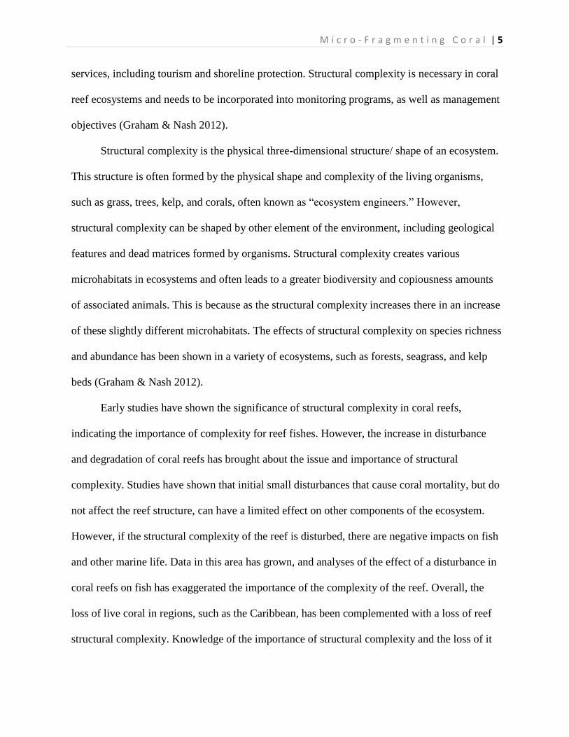
for P. clivosa and 97% variance of O. faveolata. Linear regression between the initial size of

fragments and size of the fragments after the experiment showed that the growth rates have a

correlation with colony size. Larger fragments grew faster, justifying the 56% variation in O.

faveolata and 79% in P. clivosa. Figure 4 below shows the linear (gray lines) and polynomial

(red lines) growth rate values of Orbicella faveolata (black diamonds) and Pseudodiploria

clivosa (black circles) from 9/2/2014 to 1/19/2015 and Porites lobate (black squares) from

6/25/2006 to 1/17/2007. Figure 4 below that shows (A) initial size of Orbicella faveolata versus

size after 132 days of growth; (B) initial fragment size of Pseudodiploria clivosa versus 139 days

of growth; (C) initial size fragments of Porites lobata versus size after 38 days of growth

(Forsman, Page, Toonen & Vaughan, 2015).

Figure 4. Average increase in coral area over ceramic tiles (Forsman, Page, Toonen & Vaughan, 2015)


Figure 5. Relationship between initial and final size (Forsman, Page, Toonen & Vaughan, 2015)

During a 4 month time period micro-fragments of O. faveolata increased by 293 cm2 and

P. clivosa fragments increased by 222 cm2. This approximates to ~11 cm and ~9 cm of increased

colony diameter, assuming circular colony growth. This study measured change in area covered

by thin sheets of live encrusted tissue, which would not be comparable to many field studies

because they quantify change in maximum diameter or linear extension, for example many

Caribbean corals grow 0.5-1 cm per year. Nonetheless, 89 cm2 of O. faveolata live tissue, and

136 cm2 of P. clivosa tissue, resulted in a 329 cm2 increase of tissue and 154% area increase over

four months (Forsman, Page, Toonen & Vaughan, 2015).


The growth rate of both species are within the expected bounds of linear rates of growth,

which explains the 86% and 88% variation and the second polynomial curve explained between

94% and 97% of the variance in growth rates. This showed that the growth rates of fragments

probably accelerated near the end of the experiment. Difference in growth rate could be

explained by a variety of reasons, but the initial fragment size was evidently very important,

because smaller fragments grew at a slower rate compared to larger fragments. The scope of the

experiment did not consider multiple effects of growth rate, including seasonality, temperature,

colony age, or other biotic and abiotic factors. Previous works have shown a clear

correspondence between the size of fragmented pieces and growth rates, and that larger

fragments grew at a faster rate (Forsman, Page, Toonen & Vaughan, 2015).

Care of a Salt Water Aquarium Tank

Understanding how to properly set up and care for a salt water aquarium was necessary

for maintaining a healthy, controlled environment for the coral fragments. Coral is a very fragile

species and even if everything is running properly and looks fine one day in twelve hours all of a

tank’s inhabitants could die (Jason Ryan, personal communication, October 25, 2015). First, set

up the tank, install the filtration system, and fill the aquarium with freshwater, preferably treated

by reverse osmosis. Untreated city water, if used, should be treated with a de-chlorinator in order

to remove any chlorine that could be harmful to aquarium life from the water. Next, add salt

following instructions of the salt mix used. A hydrometer can be used to monitor and raise the

salinity levels. Install the heater and set it to the desired temperature. Let the system run

independently for a few days to guarantee a proper water temperature and that the equipment is

functioning properly (Drs. Foster & Smith Educational Staff, 2015).


After the aquarium has run independently for a few days, with the equipment functioning

properly start adding aragonite-based substrate and live rock. Adding 2-3 inches of live sand that

donates beneficial bacteria and micro-organisms to the aquarium is also suggested. After placing

sand and substrate in the tank move onto adding some live rock (Drs. Foster & Smith

Educational Staff, 2015).

Live rock is a porous, aragonite-based rock that has been gathered from rubble zones of

ocean reefs and hosts large quantities of helpful bacteria and micro-organisms. Additionally, live

rock grants fish and other organisms a good hiding spot and assists in preserving healthy water

parameters. Live rock provides a tank with an aesthetic appeal as well as a natural, biological

filtration, moreover providing a necessary environment for fish and invertebrates. Add

approximately 1-1/2 pounds of live rock per gallon of water in the tank. The precise weight

should vary depending on the type of rock (Drs. Foster & Smith Educational Staff, 2015).

Before adding fish or invertebrates the live rock must be cured. Curing the live rock takes

4-5 weeks and initiates the Nitrogen Cycle. Certain people will add shrimp to their tanks to

increase the ammonia levels and kick-start the Nitrogen cycle of the tank (Jason Ryan, personal

communication, November 1, 2015). While this is going on start weekly 25% water changes. To

start curing the live rock stack the rock loosely in the aquarium, creating caves for fish to swim

through. Make sure to stack the rocks right side up, with the more colorful side facing upward,

this will allow for appropriate lighting conditions and ideal conditions for coralline algae, which

need a lot of light and sponges, which need minimal lighting. Keep the aquarium dark during this

time to enhance algae growth, limiting lighting times to only when checking the tank (Drs.

Foster & Smith Educational Staff, 2015).


Once the ammonia and nitrite levels have reached 0 ppm the live rock has fully cured and

the biological filtration system of the tank has been established. Set up a lighting system that will

be turned on for 10-12 hours a day, mirroring a normal day. There will likely be an algae bloom

for the first few weeks after lighting has been added and an algae attack pack can be used to

decrease the algae growth. Follow the instructions and the natural biological filtration system

should be able to handle new inhabitants because of the fully cured rock system. Test the

ammonia and nitrite levels again before adding any fish or invertebrates (Drs. Foster & Smith

Educational Staff, 2015).

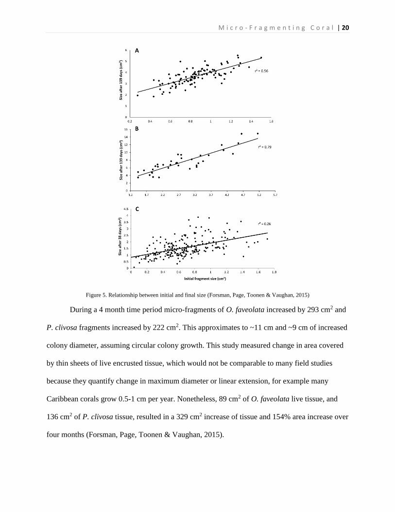
Potential for reef restoration, growth assays, and coral aquaculture

Being able to promote growth over a pre-determined substrate could help in a variety of

applications, including proliferation of rare coral species, developing standard growth assays,

coral aquaculture, and reef restoration. The ability for a coral fragment to grow on a benthic

surface, or ‘self-attach’ is necessary for the colony to survive and the transplantation to be

successful. In this experiment self-attachment of tissue spreading has been shown through a

variety of substrates. This allows for the improvement in transplantation and for the fusion

method could be used to increase to increase the likeliness of fusion over the benthic surface.

Field trials are currently in development to find procedures that effectively encourage nursery

growth coral to fuse and attach itself to the benthic surface. These experiments are testing the

utility of this method to restore O. faveolata, M. cavernosa, and P. clivosa to reefs that have been

affected by anomalous cold temperatures that occurred in early 2010.

Coral reefs are declining and this calls for more responsible coastal development. Also,

there is an increase in the demand for sustainable resources of coral materials to use for

aquacultures, research, mitigation, and restoration projects. As said by Forsman (October 2015)


“The micro-fragmentation- fusion strategy effectively manipulates the surface areas of a coral

onto a two dimensional plane, over which small colonies rapidly spread tissue and fuse.” Being

able to encrust coral onto a myriad of materials allows experiments to be done testing an

assortment of fresh methods for coral cultivation and transplantation, such as mass producing

‘seedlings.’ If a complex three dimensional structure were to be covered, then coral would be

able to successfully combine the benefits of reef restoration with artificial reefs. But, to

effectively create the maximum beneficial combination long term studies have to determine

physiological and reproductive effects of the process, and evaluate the advantages compared to

traditional direct transplantations, which often result in small fragments which are susceptible to

higher mortality rates. Although, this method could be extended to a larger scale to allow for a

more sustainable source of coral material and provide more knowledge on the cultivation of

slower growing species of coral. Incorporating in-situ, in the ocean and natural habitat, and ex-

situ, in a controlled tank, nursery plans could offer source material at scales formerly not

conceivable (Forsman, Page, Toonen & Vaughan, 2015).


Research Plan

A. Researchable question:

How does the original size of micro-fragmented pieces of Montipora capricornis

affect the two-dimensional cross section area growth rate of the coral?

B. Hypothesis:

If one large piece of Montipora capricornis is micro-fragmented into smaller

pieces ranging from 0-6 sq. cm cross-sectional area, then the larger pieces will

have a faster growth rate compared to smaller pieces of coral.

C. Description in detail of methods or procedures

To perform this experiment, a tank was set up to place the micro-fragmented coral in.

After visiting an aquarium store and talking with employees there, who have extensive

experience with setting up tanks and maintaining them, the tank that was selected to be used was

a 29-gallon bio-cube that contains filters, lights, and everything else needed to maintain a tank,

besides a heater incorporated into the tank. The tank was set-up according to the instructions of

the aquarium store, and other reliable sources.

One piece of Monitpora capricornis will be micro-fragmented into various sizes between

0.5 cm2, and 6.0 cm2 using a saw at Jay’s Aquatics. The fragments were be epoxied with a

marine super-glue on an aragonite substrate plug that was much bigger than fragment, in order

for coral fragments to have room to grow. Plugs will be labeled with letters according to size and

placed randomly in the tank. The tank was be regulated by snails (Margaritea pupillus) and

hermit crabs (Calcinus spp.) that will clean the algae and act as a bio-filter maintaining the

environment within the tank. Once the tank had established a healthy environment, one kenya

tree (Capnella spp.) was added, to ensure that hard corals, which are more finicky than soft


corals, would survive in the tank. After the soft coral has survived for one week the micro-

fragmented coral was brought in.

The process for micro-fragmenting coral involved using a saw to cut between polyps and

get an approximate size. The “goal” sizes, between 0.5 cm2, and 5.0 cm2, but the exact

topographic surface area will be measured for each fragment and recorded. Different sizes were

taken from different regions of the coral, and from different pieces of coral to ensure that that

fragments did not grow at different rates because of the original poor health of a single coral

piece. These fragments were then attached to an aragonite plug substrate with epoxy, then

transported to the 29-gallon tank. The fragments were placed in the tank an even distance apart

and each size will occupy different sections of the tank.

The tank was be checked daily for temperature, as well as a visual check of the health of

the tank, this includes algal growth, checking the filter, and making sure each coral fragment

looks healthy. Weekly chemical tests of ammonia, nitrites, nitrates, pH, magnesium, alkalinity,

and calcium were performed. If a coral fragment fell off of the substrate then it was included in

final calculations of growth rate. Fragments that died were not included in the study. The action

of micro-fragmenting is very aggressive and coral can die simply from going through the

process, which is why the fragments that died initially were not included. Every two weeks a

picture of the coral fragments was be taken with a camera, and a ruler will be placed next to the

coral fragments for reference.

At the conclusion of the experiment the percentage increase of each fragment was

calculated. The average of each was be calculated to calculate the average percent increase for

each original size of coral fragments. The final results will be based on the average growth rate,


not on the percent, and whether or not there is a notable difference between the starting sizes of

coral fragments in the species of coral.


Methodology

Setting up the tank

A 29-gallon BioCube® tank designed by Corallife® was acquired from Jay’s Aquatics.

The dimensions of the tank are 50.80 cm (l) by 53.34 cm (w) by 47.31 cm (h). The tank came

with build in lighting, which included one 36 Watt Actinic Blue Straight Pin, one 36 Watt

10,000K Daylight Straight Pin, and one 0.75 Watt Lunar Blue LED Bar. The tank also had a 60

mm, 15.83 CFM, 25.5 Db cooling fan, and a pump with a 1000 L/hour flow rate.

The tank was then slowly filled with pre-made salt water from Jay’s Aquatics in 5 gallon

increments. After the first 5 gallons were added one 9.072 kg bag of black Nature’s Ocean® Bio-

Activ Live® Aragonite Reef Sand was placed in the bottom of the tank. Six pieces of live rock

weighing a total of 8.50 kg were spread out across the bottom of the tank. The remaining 15

gallons of water were added to the tank. A 150W Marina® Submersible Aquarium Heater was

placed in the tank, as well as a Deep Blue Professionals ProTherm™ digital thermometer on the

opposite side of the tank. Lastly, 30 mL of API® Aquarium Pharmaceuticals Quick Start® was

added to the tank.

Three days after the tank was set up, 2 dead jumbo shrimp were added to the tank in

order to jump start the Nitrogen cycle. After 36 hours, the shrimp were removed and the tank

took a week after that to “cycle,” until the ammonia and nitrite levels were both at 0 ppm. Three

days later 12 Calcinus spp., red legged hermit crabs and 12 Margarites pupillus, Margarita

Snails were added to the tank, and the 0.75 Watt Lunar Blue LED Bar and 36 Watt Actinic Blue

Straight Pin were set to stay on for 4 hours a day. The amount of flight was increased over the

next week until it was set to 12 hours of light. A Capnella spp. coral was placed in the tank to

ensure that chemical levels were at the correct level for coral.


Maintaining Tank

Four weeks after setting up the tank measurements of pH, ammonia, nitrites, nitrates,

magnesium, alkalinity, and calcium were only taken once a week. The pH, ammonia, nitrates,

and nitrites were found using the API™ Aquarium Pharmaceuticals Saltwater Master Test Kit.

Image 1. API™ Aquarium Pharmaceuticals Saltwater Master Test Kit.

The magnesium, alkalinity, and calcium were found using the Red Sea Reef Foundation

Pro Test Kit.


Image 2. Red Sea Reef Foundation Test Kit (amazon.com).

Red Sea Reef Foundation C Mg Supplement, Red Sea Reef Foundation B Buffer

Supplement, and Red Sea Reef Foundation A Ca/Sr Supplement were added for magnesium,

alkalinity, and calcium supplements, respectively, according to the charts. It was calculated that a

maximum of 8.0 mL of Mg Supplement could be added per day, 11.1 mL of Buffer Supplement

per day, and 8.0 mL of Ca Supplement per day, based on the 20-gallon tank.

Image 3. Testing chemicals in the tank.


Image 4. Reef Foundation C Mg Supplement chart (SwellUK.com)

Image 5. Reef Foundation B Buffer Supplement chart (SwellUK.com)

Image 6. Reef Foundation A Ca/Sr Supplement chart (SwellUK.com)


A bi-weekly 25% water change was performed throughout the experiment, and the filter

was change every 4 weeks. The pump for the filter was taken out over 4 weeks and cleaned. The

two blue lights (36 Watt Actinic Blue Straight Pin, and 0.75 Watt Lunar Blue LED Bar) were left

on from 6 am to 6 pm for 12 hours every day, and the white light used occasionally for

observation.

Sixty-eight days after the tank was set up, 2.0 mL of API™ Aquarium Pharmaceuticals

Algae Fix® Marine Algaecide were added every three days to control the green film algae that

had grown on the side of the tank. The algae was also scraped off the side of the tank using a dull

razor blade. Four Trochus maculatus were added to maintain the algae. The solution was added

accordingly when algae started to accrue, but there was minimal usage.

Fragmenting Coral

A decision matrix was utilized to select the best option to micro-fragment coral.

Table 2. Decision Matrix for coral species

A large piece (15 cm by 25 cm) of Montipora capricornis coral was broken off of the

rock that it was attached to, using scissors to lever it off. This resulted in seven large pieces

which were further fragmented into sizes between 0.73 cm2 - 5.57 cm2 using a band saw. A

picture was taken of each fragment with a cm ruler in the frame for reference. The 2-D basic

measurements of each fragment was also found, and each frag was labelled with an approximate

number of square centimeters 1, 1.5, 2, 2.5, and +, for all fragments over 3 cm2. These

Criteria Weight Cyphastrea Astreopora Montipora Capricornis Capnella sp. Seriatopora hystrix

Polyp size/ shape 7 8 6 9 3 4

natural growth rate 7 5 5 7 8 8

original size 5 7 6 10 5 4

potential for reef

restoration 7 7 8 6 2 3

Amount in aquatic

store 9 2 0 8 6 4

Total 193 163 276 170 161


measurements were not used for the actual measurements, only an approximation for

identification purposes. The fragments were also labelled with letters, such as 1A, 1B, and so on

for individual identification. The identification of each frag was then written on Boston Aqua

Farms ceramic reef discs with a graphite pencil. The fragments were then attached to the ceramic

reef disks using a small dollop of Seachem® Cyanoacrylate Adhesive Reef Glue™.

Finding Exact Measurements of Coral

The exact measurements of the coral could not have been found using calipers, because

of the irregular shape of most of the fragments. In order to find the exact measurements the photo

imaging app GIMP was used. The photo of each fragment at each specific timing was imported

into GIMP. The area of the circle was then selected, free-hand, using the free-select tool, and the

area of the coral found in pixels using the histogram tool. Then the length of 1 cm was found in

pixels by measuring 1 cm using the measuring tool. There could be some errors with extremely

precise measurements, but it is assumed that if any errors were made then they were repeated

errors since the same person was taking all of the measurements, and the results would not be

affected, because the error would be made for each analysis of each picture. The total number of

pixels was then divided by the length of 1 cm in pixels squared to find the area of each fragment

in cm2.

When taking the original measurements white pieces of coral were not selected, because

they did not cover the surface area of the original piece of M. capricornis. Later on these white

pieces did turn brown, and were then included in the area because it was an increase in the

topical area of the piece of coral. Sections of coral that had died were not included, if that piece

of coral was continuing to grow. If glue had covered a portion of the coral then that piece was

not included in the data set, because the glue inhibited growth and could interfere with the other


sections of the coral, not just the portion that it covered. If it was obvious that a piece of coral

had deceased then it was not counted in the results.


Results

The growth rate, as well as the percent growth rate, area increase, and percent area

increase, of 39 micro-fragmented pieces of coral was calculated 68 days after the initial micro-

fragmentation.

Table 3. Results of the growth rate, percent growth rate, area increase, and percent area increase of fragmented pieces of

Montipora capricornis.

<1

cm2

1-1.5

cm2

1.5-2

cm2

2-2.5

cm2

2.5-3

cm2

3-4

cm2

4-6

cm2

Day 1 cm2 0.869 1.207 1.740 2.243 2.750 3.109 4.933

Day 68 cm2 2.850 3.698 4.759 4.952 6.524 7.181 9.407

growth

rate cm2/day 0.029 0.037 0.044 0.040 0.055 0.060 0.068

%

growth

rate

% area

increase/

days

4.960 4.503 4.043 3.253 3.445 3.394 2.908

area

increase

final cm2 -

initial cm2 1.981 2.491 3.026 2.704 3.759 4.072 4.643

% area

increase

final cm2 /

initial cm2 337.3 306.2 274.9 221.2 234.3 230.8 197.8


Figure 6. A scatter plot that represents how the growth rate is affected by the initial size.

Overall the large pieces of coral (avg. 4.933 cm2 ± 0.897 cm2) had a faster growth rate, at

0.068 cm2/ day ± 0.011 cm2/ day compared to the smallest pieces of coral (avg. 0.869 cm2 ±

0.121 cm2) which had a growth rate of 0.029 cm2/day ± 0.011 cm2/ day. That is 234% faster in

the largest setting of micro-fragmented pieces of coral.

y = -0.0013x2 + 0.0172x + 0.0159R² = 0.9219

0.015

0.025

0.035

0.045

0.055

0.065

0.075

0.085

0.5 1.5 2.5 3.5 4.5 5.5

Gro

wth

Rat

e (c

m2/d

ay)

Initial Size (cm2)

Growth Rate vs. Initial Size

y = 0.1588x2 - 1.3926x + 5.9635R² = 0.9322

2.0

2.5

3.0

3.5

4.0

4.5

5.0

5.5

6.0

6.5

0.5 1.5 2.5 3.5 4.5 5.5

Per

cen

t G

row

th R

ate

Initial Size (cm2)

Percent Growth Rate vs. Initial Size


Figure 7. This graph represents the percent that each coral setting grew per day. Percent growth is the percent growth (final

size/initial size) over the number of days (68).

As the initial size of the coral increased the percent growth decreased. This relationship

resulted in a polynomial line of best fit, with an r-squared value of 0.93.

Figure 8. The area increase (cm2) dependent upon the initial size (cm2) of the coral fragments.

The area increase (final size cm2 – initial size cm2) was dependent upon the initial

fragmented size of the coral, with a polynomial relationship that had an r-squared value of 0.92.

y = -0.0898x2 + 1.1728x + 1.081R² = 0.9219

1.0

1.5

2.0

2.5

3.0

3.5

4.0

4.5

5.0

5.5

6.0

0.5 1.5 2.5 3.5 4.5 5.5

Are

a In

crea

se (

cm2 )

Initial Size (cm2)

Area Increase vs. Initial Size


Figure 9. This graph represents the percent increase over the 68 days of the experiment. Percent increase was based on the final

size divided by the initial size.

As the initial size of the coral fragments increased the percentage growth decreased, even

though they had a higher overall increase in area. There was a strong polynomial relationship

between the initial size and the percent area increase, with an r-squared value of 0.93. The largest

setting had the smallest percent area increase, which was still almost 200% (actual 197.8% ±

13.02%) of the initial size of the coral fragment.

y = 10.796x2 - 94.698x + 405.52R² = 0.9322

125

175

225

275

325

375

425

0.5 1.5 2.5 3.5 4.5 5.5

Per

cen

t A

rea

Incr

ease

Initial Size (cm2)

Percent Area Increase vs. Initial Size


Figure 10. A graph of the initial size of the fragments compared to the final size of the fragments.

The relationship between the initial and final size of coral fragments is a polynomial

relationship, with an r-squared value of 0.99.

Figure 11. A scatterplot of all the fragments of coral and each individual growth rate after 68 days.

y = -0.1108x2 + 2.2571x + 1.0114R² = 0.9857

2.0

3.0

4.0

5.0

6.0

7.0

8.0

9.0

10.0

11.0

0.5 1.5 2.5 3.5 4.5 5.5

Fin

al S

ize

(cm

2 )

Initial Size (cm2)

Final Size vs. Inital Size

y = -0.0009x2 + 0.0157x + 0.0179R² = 0.4222

0.01

0.02

0.03

0.04

0.05

0.06

0.07

0.08

0.09

0.5 1.5 2.5 3.5 4.5 5.5

Gro

wth

Rat

e (c

m2 /

day

)

Initial Size (cm2)

Growth Rate vs. Initial Size


There was a moderate correlation between the initial size of fragments, and the growth

rate, with an r-squared value of 0.42. Overall there is a visible trend of an increase in growth rate

as the initial size of fragments increased, which is seen more clearly on figure 6.

Figure 12. A scatterplot of the growth rate of each range of coral fragments with polynomial lines of best fit.

There was not a consistent change in the growth rate from day 17 to day 68. None of the

growth rates remained constant, nor did any of them increase or decrease linearly. Three settings

(1–1.5 cm2, 2.5-3 cm2, and 4-6 cm2) had a negative polynomial line of best fit, with r-squared

values of 0.56, 0.76, and 0.85, respectively.

0.020

0.025

0.030

0.035

0.040

0.045

0.050

0.055

0.060

0.065

0.070

0 10 20 30 40 50 60 70

Gro

wth

Rat

e (c

m2 /

day

)

Day

Growth Rate vs. Day

<1 cm2

1-1.5 cm2

1.5-2 cm2

2-2.5 cm2

2.5-3 cm2

3-4 cm2

4 - 6cm2

Poly. (<1 cm2)

Poly. (1-1.5 cm2)

Poly. (1.5-2 cm2)

Poly. (2-2.5 cm2)

Poly. (2.5-3 cm2)

Poly. (3-4 cm2)

Poly. (4 - 6cm2)


Figure 13. The average growth rate per day of all fragments.

The average growth rate of all the fragments remained mostly constant, approximately

0.044 cm2/ day for the first 46 days, and only increasing to 0.048 cm2/day after 68 days.

y = 3E-06x2 - 0.0002x + 0.0472R² = 0.971

y = 5E-06x2 - 0.0003x + 0.0359R² = 0.9748

0.020

0.025

0.030

0.035

0.040

0.045

0.050

0.055

0.060

0.065

0.070

0 10 20 30 40 50 60 70

Gro

wth

Rat

e (c

m2 /

day

)

Day

Average Growth Rate vs. Day

Average 0-2.5 sq. cm 2.5-6 sq. cm

Poly. (Average) Poly. (0-2.5 sq. cm)


Data Analysis and Discussions

The data showed that the largest pieces (avg. 4.933 cm2 ± 0.897 cm2) grew at a rate 234%

faster than the smallest pieces (avg. 0.869 cm2 ± 0.121 cm2), and there was a polynomial trend

with an r-squared value of 0.92, showing a strong correlation. The percent growth rate decreased

as the initial size increased, which is because although the smaller pieces overall had a slower

growth rate it was a much larger percent of their original size. Any small increase in smaller

pieces of fragments would have a much higher percent increase, just because some of these

fragments started at much smaller sizes. This experiment was looking for a faster growth rate,

because a faster growth rate meant that the coral would be asexually reproducing faster.

The percent increase is size decreased as the initial micro-fragmented size increased. The

smaller pieces had a smaller increase in size, but relative to their original sizes it was larger

compared to the larger initial sizes, which is why this trend is seen. The goal of this experiment

was to find the ideal size to micro-fragment coral, and the size that had the largest increase in

area would be preferable. The percentage is not important, because the overall increase in area

has a higher priority than a higher percentage increase.

The maximum value for this polynomial line of best fit is 6.62 cm2, which is outside of

the range of data. The line of best fit for the scatterplot of each individual fragment had a

maximum initial size value of 8.72 cm2. Because the range of data tested did not extend this far it

is unsure to conclude that these are the best sizes to micro-fragment pieces of Montipora

capricornis.

The growth rate did increase overall, from 0.044 cm2/ day to 0.048 cm2/day. This was

only a 9% increase, and was not seen across the individual fragment settings. It was observed


that the three highest settings (2.5-3 cm2, 3-4 cm2, and 4-6 cm2) overall had a significantly higher

growth rate, 184% faster (approximately 0.03 cm2/ day more). There also did not seem to be a

trend between the average of the larger three groups, but there was a strong polynomial

relationship between the smaller four settings (<1 cm2, 1-1.5 cm2, 1.5-2 cm2, and 2-2.5 cm2) and

the average growth rate, with r-squared values of 0.97 for both.


Conclusion

The increase in area, both percentage and overall area shows that micro-fragmenting is a

legitimate method of propagating coral growth. The polynomial line chosen for the growth rate

vs. initial size, with the averaged data, was chosen because it is likely that the curve would

decrease once the coral was micro-fragmented to a certain large size. This is because there is a

point where fragmented pieces of coral would not be small enough to have the necessity of

increasing their size rapidly. The overall increase in size was also calculated to have a positive

trend, with the size difference increasing as the initial size increased. This is most likely because

the growth rate was higher in the larger pieces of coral. The fragments of coral grew to double,

or more of their original size in only 68 days. The growth rate increased overall, but there was no

increase in the larger pieces of coral. Contrastingly the smaller pieces increased their growth rate

in a polynomial trend upward. The growth rate was higher in the larger fragments, and increased

as the size of fragments also increased, which proved the hypothesis, that larger pieces of micro-

fragmented Montipora capricornis would have a greater growth rate (cm2/day) compared to

smaller micro-fragmented pieces.


Assumptions and Limitations

In order to conduct this experiment assumptions had to be made. First, it was assumed

that M. capricornis would only grow two-dimensionally, covering a larger area. Also, that the

initial 3-D height would not affect the growth rate. The overall shape of the original piece of

coral was also assumed to not affect the growth rate. The conditions of the tank were considered

to be consistent throughout the floor of the tank, because the fragments were not rearranged

during the experiment. It was also assumed that because the fragments came from the same

parent coral, with the same DNA, they would all start with the same growth rate, no matter their

location within the coral. If the fragmented pieces fell off of the ceramic reef disk it was assumed

that it would not affect their growth rate, because they were reattached five days later and the rest

of the pieces were not growing, only recovering from the trauma of micro-fragmentation. This

project was limited by time constraints, as well as the amount of coral available from a single,

large piece at Jay’s Aquatic Store.


Future Applications

The work of this experiment suggests that the ideal size to micro-fragment coral is either

around or above 5 cm2. Future applications include using a different species of coral and

performing a similar experiment to deduce how the initial micro-fragmented size affected its

growth. This experiment could be run again, with a larger, higher range of initial fragment size

from 5 cm2 – 10 cm2, instead of 0 cm2 – 5 cm2. Testing how well the pieces of coral fuse

together, and seeing if coral from the same species, but different parent corals would fuse

together is another extension of this work. Extending the length of time for a similar project, and

seeing how the growth rate changes with time.


Literature Cited

Calfo, A (2002). Coral Fragmenting: Not Just for Beginners. Reefkeeping.

Forsman, Zac H., Page, Christopher A., Toonen, Rober J., & Vaughan. (20 Oct. 2015). Growing

coral larger and faster: micro-colony-fusion as a strategy for accelerating coral cover.

PeerJ. doi: 10.7717/peerj.1313.

Graham, N. A. J., & Nash, K. L. (26 Nov 2012). The importance of structural complexity in

coral reef ecosystems. Coral Reefs, 32, 315–326. doi: 10.1007/s00338-012-0984-y.

McCalmon, Iain. (May 2014). The Coral Grief. ScietificAmerican.com, May 2014, 66-69.

Morin, Richard. (2014, November 23). A Lifesaving Transplant for Coral Reefs. The New York

Times. n.p.

Osinga, R., Schutter, M., Griffioen, B., Wijffels, R. H., Verreth, J. A. J., Shafir, S., Henard, S., et

al. (17 May 2011). The Biology and Economics of Coral Growth. 10.1007/s10126-011-

9382-7.

Williams, Dana E., and Miller, Margaret W. (Nov. 2010). Stabilization of Fragments to Enhance

Asexual Recruitment in Acropora Palmata, a Threatened Caribbean Coral. Restoration

Ecology (pp. 446-451). DOI: 10.1111/ 1526-100X.2009.00579.

http://www.ncbi.nlm.nih.gov/pubmed/?term=Forsman%20ZH%5Bauth%5D

http://www.ncbi.nlm.nih.gov/pubmed/?term=Page%20CA%5Bauth%5D

http://www.ncbi.nlm.nih.gov/pubmed/?term=Toonen%20RJ%5Bauth%5D

http://www.ncbi.nlm.nih.gov/pubmed/?term=Vaughan%20D%5Bauth%5D


Appendix

Table 4. Raw Data after 68 days, organized by size.

1 B 1.5 C 1 I 1 E 1 F 1 H AVG STDEV % RSD

Day 1 0.7283 0.75893 0.79457 0.96255 0.98313 0.98553 0.86884 0.12067 13.8889

Day 17 0.99057 1.31059 1.5046 1.39683 1.15781 1.23863 1.2665 0.1813 14.3149

Day 32 1.51393 1.79707 1.88923 1.7041 1.49885 1.38448 1.63128 0.19573 11.9985

Day 46 1.90628 2.14597 2.50858 2.269 1.70239 1.55488 2.01452 0.3596 17.8502

Day 61 2.23575 2.49574 3.31944 2.92374 1.77192 1.86589 2.43541 0.60466 24.8277

Day 68 2.82818 2.72096 3.94159 3.33212 2.38839 1.88986 2.85018 0.71779 25.1839

growth rate 170.01543 0.03245 0.04177 0.02555 0.01028 0.01489 0.02339 0.0121 51.7278

growth rate 320.02455 0.03244 0.03421 0.02317 0.01612 0.01247 0.02383 0.00862 36.1745

growth rate 460.02561 0.03015 0.03726 0.0284 0.01564 0.01238 0.02491 0.00934 37.4843

growth rate 61 0.02471 0.02847 0.04139 0.03215 0.01293 0.01443 0.02568 0.01083 42.1722

growth rate 68 0.03088 0.02885 0.04628 0.03485 0.02067 0.0133 0.02914 0.01142 39.1971

% growth rate 5.71068 5.27243 7.29504 5.09082 3.57261 2.82 4.96026 1.58966 32.0479

area increase 2.09988 1.96203 3.14701 2.36957 1.40526 0.90433 1.98135 0.77663 39.1971

% area increase 388.326 358.525 496.063 346.175 242.937 191.76 337.298 108.097 32.0479

2 I 1 D 1 C 1 A 2.5 G 1.5 E 2 E AVG STDEV

Day 1 1.0722 1.19376 1.19804 1.20212 1.24483 1.26754 1.26938 1.20684 0.06762 5.6032

Day 17 1.29538 1.59159 1.73183 1.53995 1.68711 1.99559 2.26782 1.72989 0.31775 18.3683

Day 32 1.89202 2.17524 2.33673 3.12586 2.09195 2.23634 2.93405 2.39889 0.45576 18.9988

Day 46 2.19135 2.36951 2.58581 3.63101 2.58703 2.41984 3.45966 2.74917 0.56261 20.4647

Day 61 2.74162 3.22264 3.28243 4.57148 3.37207 3.08035 4.20841 3.497 0.65086 18.612

Day 68 3.14003 3.53699 3.00208 4.79078 3.6046 3.3143 4.49587 3.69781 0.68414 18.5011

growth rate 17 0.01313 0.0234 0.0314 0.01987 0.02602 0.04283 0.05873 0.03077 0.01546 50.2547

growth rate 32 0.02562 0.03067 0.03558 0.06012 0.02647 0.03028 0.05202 0.03725 0.01346 36.1357

growth rate 46 0.02433 0.02556 0.03017 0.0528 0.02918 0.02505 0.04761 0.03353 0.01169 34.8692

growth rate 61 0.02737 0.03326 0.03417 0.05524 0.03487 0.02972 0.04818 0.03754 0.01023 27.2458

growth rate 68 0.03041 0.03446 0.02653 0.05277 0.0347 0.0301 0.04745 0.03663 0.00974 26.5949

% growth rate 4.30673 4.35721 3.68503 5.86069 4.25831 3.84521 5.20852 4.5031 0.77055 17.1116

area increase 2.06783 2.34323 1.80404 3.58866 2.35976 2.04676 3.22649 2.49097 0.66247 26.5949

% area increase 292.858 296.29 250.582 398.527 289.565 261.475 354.179 306.211 52.3975 17.1116


1.5 D 2.5 H 2.5 E 2.5 C 2 F 1.5 B 2.5 B 2 A +O AVG STDEV

Day 1 1.54447 1.59761 1.65674 1.67437 1.70582 1.76048 1.76415 1.92393 1.97012 1.73308 0.14066 8.11595

Day 17 2.00578 2.47862 2.11718 2.36408 2.31596 2.27795 2.39678 2.95187 2.30888 2.35745 0.26491 11.237

Day 32 2.58268 3.10421 2.41001 2.4659 2.49187 2.97546 3.33941 3.51211 3.37992 2.91795 0.43852 15.0283

Day 46 3.20009 3.31189 2.92375 2.88649 2.74471 3.76645 3.64886 4.05635 3.7614 3.36667 0.46304 13.7537

Day 61 4.16312 4.68446 3.08975 4.14871 2.78238 4.87128 3.784 5.57262 4.37989 4.16402 0.86671 20.8142

Day 68 4.55013 5.67575 3.49014 4.79228 3.06053 5.83676 4.37896 6.56855 4.47468 4.75864 1.12034 23.5433

growth rate 17 0.02714 0.05182 0.02708 0.04057 0.03589 0.03044 0.03721 0.06047 0.01993 0.03673 0.01282 34.894

growth rate 32 0.03244 0.04708 0.02354 0.02474 0.02456 0.03797 0.04923 0.04963 0.04406 0.03703 0.011 29.714

growth rate 46 0.03599 0.03727 0.02754 0.02635 0.02258 0.04361 0.04097 0.04636 0.03894 0.03551 0.00824 23.1902

growth rate 61 0.04293 0.0506 0.02349 0.04056 0.01765 0.051 0.03311 0.05981 0.0395 0.03985 0.01348 33.8348

growth rate 68 0.0442 0.05997 0.02696 0.04585 0.01992 0.05995 0.03845 0.0683 0.03683 0.04449 0.01602 36.0085

% growth rate 4.33248 5.22448 3.09798 4.20903 2.63848 4.87563 3.65029 5.02079 3.3401 4.04325 0.91314 22.5844

area increase 3.00567 4.07814 1.8334 3.11791 1.35471 4.07628 2.61481 4.64462 2.50456 3.02556 1.08946 36.0085

% area increase 294.608 355.265 210.663 286.214 179.417 331.543 248.22 341.414 227.127 274.941 62.0937 22.5844

2.5 D + M 2.5 F AVG STDEV

Day 1 2.19297 2.2427 2.30784 2.24784 0.05761 2.56292

Day 17 2.5649 2.40911 3.60987 2.86129 0.65295 22.8201

Day 32 3.49509 2.25573 3.45689 3.06923 0.70478 22.9626

Day 46 4.52334 2.79031 4.01152 3.77506 0.89039 23.586

Day 61 5.11678 3.634 4.1334 4.29473 0.75444 17.5667

Day 68 6.72775 3.64897 4.47877 4.95183 1.59297 32.1694

growth rate 17 0.02188 0.00979 0.07659 0.03609 0.03559 98.6398

growth rate 32 0.04069 0.00041 0.03591 0.02567 0.02201 85.7373

growth rate 46 0.05066 0.0119 0.03704 0.0332 0.01966 59.2181

growth rate 61 0.04793 0.02281 0.02993 0.03356 0.01295 38.5889

growth rate 68 0.06669 0.02068 0.03193 0.03976 0.02398 60.3167

% growth rate 4.51158 2.3927 2.85393 3.25274 1.11431 34.2577

area increase 4.53478 1.40626 2.17093 2.70399 1.63096 60.3167

% area increase 306.787 162.704 194.067 221.186 75.7733 34.2577

+N 2.5 A + D +L + G + F AVG STDEV

Day 1 2.60812 2.63401 2.65442 2.84206 2.86906 2.98595 2.7656 0.15465 5.59181

Day 17 3.28106 3.15246 2.92807 4.21053 4.24449 4.76066 3.76288 0.73886 19.6355

Day 32 3.53949 3.88062 4.32365 5.31629 5.09632 5.75632 4.65211 0.87164 18.7363

Day 46 4.19906 4.42536 4.93098 5.92172 6.47149 6.44498 5.39893 1.01237 18.7512

Day 61 4.58224 5.33414 5.40192 7.83732 6.80416 7.76194 6.28695 1.37433 21.86

Day 68 5.03389 5.29133 5.77328 7.91363 6.58118 8.55191 6.52421 1.43877 22.0528

growth rate 17 0.03958 0.0305 0.0161 0.0805 0.08091 0.10439 0.05866 0.03473 59.2089

growth rate 32 0.02911 0.03896 0.05216 0.07732 0.0696 0.08657 0.05895 0.02259 38.3106

growth rate 46 0.03459 0.03894 0.04949 0.06695 0.07831 0.0752 0.05725 0.01881 32.8561

growth rate 61 0.03236 0.04426 0.04504 0.08189 0.06451 0.0783 0.05773 0.02019 34.9768

growth rate 68 0.03567 0.03908 0.04587 0.07458 0.05459 0.08185 0.05527 0.01905 34.4667

% growth rate 2.83836 2.95419 3.19848 4.09481 3.3733 4.21185 3.44517 0.58054 16.8508

area increase 2.42577 2.65732 3.11886 5.07158 3.71212 5.56597 3.7586 1.29547 34.4667

% area increase 193.008 200.885 217.497 278.447 229.384 286.406 234.271 39.4767 16.8508


Table 5. Summarized Data with STDEV

2 C + H + I + E + B AVG STDEV

Day 1 3.02762 3.07711 3.12564 3.13987 3.17402 3.10885 0.05722 1.8406

Day 17 4.21096 3.89166 5.34754 3.39303 4.36246 4.24113 0.72132 17.0076

Day 32 5.55357 4.68737 5.85415 4.17302 4.62936 4.97949 0.69873 14.0322

Day 46 5.4479 5.24997 6.84817 4.8748 6.17746 5.71966 0.7892 13.7981

Day 61 6.46735 6.03004 7.76963 6.31741 7.56602 6.83009 0.78403 11.4791

Day 68 6.79762 5.91543 8.63241 7.10939 7.44838 7.18065 0.99144 13.8072

growth rate 17 0.06961 0.04791 0.1307 0.01489 0.06991 0.0666 0.04228 63.485

growth rate 32 0.07894 0.05032 0.08527 0.03229 0.04548 0.05846 0.02268 38.7984

growth rate 46 0.05261 0.04724 0.08092 0.03772 0.06529 0.05676 0.01679 29.5782

growth rate 61 0.05639 0.04841 0.07613 0.05209 0.072 0.061 0.01234 20.2285

growth rate 68 0.05544 0.04174 0.08098 0.05838 0.06286 0.05988 0.01419 23.6941

% growth rate 3.30177 2.82706 4.06149 3.32975 3.45098 3.39421 0.44239 13.0337

area increase 3.77 2.83833 5.50678 3.96952 4.27436 4.0718 0.96478 23.6941

% area increase 224.52 192.24 276.181 226.423 234.667 230.806 30.0826 13.0337

+A + K + J AVG STDEV

Day 1 4.29874 4.42727 5.56705 4.76435 0.69812 14.6531

Day 17 4.97466 6.18129 6.05441 5.73679 0.66306 11.558

Day 32 6.57656 7.05625 6.99617 6.87633 0.26134 3.80054

Day 46 7.66778 7.41881 8.08586 7.72415 0.33708 4.36397

Day 61 9.13798 8.45012 9.12647 8.90486 0.39386 4.42294

Day 68 9.10261 8.23499 10.8834 9.407 1.3502 14.3531

growth rate 17 0.03976 0.10318 0.02867 0.0572 0.0402 70.2779

growth rate 32 0.07118 0.08216 0.04466 0.066 0.01928 29.2091

growth rate 46 0.07324 0.06503 0.05476 0.06434 0.00926 14.393

growth rate 61 0.07933 0.06595 0.05835 0.06788 0.01062 15.6496

growth rate 68 0.07065 0.056 0.07818 0.06827 0.01128 16.5236

% growth rate 3.11398 2.73538 2.87495 2.90811 0.19146 6.5838

area increase 4.80387 3.80772 5.31636 4.64265 0.76713 16.5236

% area increase 211.751 186.006 195.497 197.751 13.0196 6.5838

<1 cm2 STDEV 1-1.5 cm2 STDEV 1.5-2 cm2 STDEV 2-2.5 cm2 STDEV 2.5-3 cm2 STDEV 3-4 cm2 STDEV 4 - 6cm2 STDEV

Day 1 cm2 0.869 0.121 1.207 0.068 1.740 0.141 2.243 0.058 2.750 0.155 3.109 0.057 4.933 0.698

Day 68 cm2 2.850 0.718 3.698 0.684 4.759 1.120 4.952 1.593 6.524 1.439 7.181 0.991 9.407 1.350

growth

ratecm2/day 0.029 0.011 0.037 0.010 0.044 0.016 0.040 0.024 0.055 0.019 0.060 0.014 0.068 0.011

% growth

rate

% area

increase/

days

4.960 1.590 4.503 0.771 4.043 0.913 3.253 1.114 3.445 0.581 3.394 0.442 2.908 0.191

area

increase

final cm2 -

initial

cm2

1.981 0.777 2.491 0.662 3.026 1.089 2.704 1.631 3.759 1.295 4.072 0.965 4.643 0.767

% area

increase

final

cm2/

initial

cm2

337.3 108.1 306.2 52.40 274.9 62.09 221.2 75.77 234.3 39.48 230.8 30.08 197.8 13.02


Acknowledgements

The author would like to thank her teachers and advisors, Mr. Ellis and Ms. Borowski for

helping her with any issues that she ran into and always being confident that the experiment

would work out. She would also like to thank her parents for assisting in setting up the tank, as

well as providing the funding to begin this experiment, and quite a feew rides to Salem, NH. The

author would like to thank Jason Ryan and Jay’s Aquatics for assisting her with all the supplies

and coral advice that she needed. The author would also like to thank David Wollensak for

looking after the tank while she was on vacation, as well as being a quality member of the coral

crew from Mr. Ellis’ advisory.

Documents

Micro-Fragmenting as a Method of Reef Restoration using · Micro-Fragmenting as a Method of Reef Restoration using Montipora capricornis Hannah Boyce MASSACHUSETTS ACADEMY OF MATH