Work ing PaPer Ser ieSno 1619 / november 2013

micro and macro analySiS on HouSeHold income, WealtH

and Saving in tHe euro area

Juha Honkkila and Ilja Kristian Kavonius

In 2013 all ECB publications

feature a motif taken from

the €5 banknote.

note: This Working Paper should not be reported as representing the views of the European Central Bank (ECB). The views expressed are those of the authors and do not necessarily reflect those of the ECB.

HouSeHold Finance and conSumPtion netWork

© European Central Bank, 2013

Address Kaiserstrasse 29, 60311 Frankfurt am Main, GermanyPostal address Postfach 16 03 19, 60066 Frankfurt am Main, GermanyTelephone +49 69 1344 0Internet http://www.ecb.europa.euFax +49 69 1344 6000

All rights reserved.

ISSN 1725-2806 (online)EU Catalogue No QB-AR-13-116-EN-N (online)

Any reproduction, publication and reprint in the form of a different publication, whether printed or produced electronically, in whole or in part, is permitted only with the explicit written authorisation of the ECB or the authors.This paper can be downloaded without charge from http://www.ecb.europa.eu or from the Social Science Research Network electronic library at http://ssrn.com/abstract_id=2358467.Information on all of the papers published in the ECB Working Paper Series can be found on the ECB’s website, http://www.ecb.europa.eu/pub/scientific/wps/date/html/index.en.html

Household Finance and Consumption NetworkThis paper contains research conducted within the Household Finance and Consumption Network (HFCN). The HFCN consists of survey specialists, statisticians and economists from the ECB, the national central banks of the Eurosystem and a number of national statistical institutes.The HFCN is chaired by Gabriel Fagan (ECB) and Carlos Sánchez Muñoz (ECB). Michael Haliassos (Goethe University Frankfurt ), Tullio Jappelli (University of Naples Federico II), Arthur Kennickell (Federal Reserve Board) and Peter Tufano (University of Oxford) and act as external consultants, and Sébastien Pérez Duarte (ECB) and Jiri Slacalek (ECB) as Secretaries.The HFCN collects household-level data on households’ finances and consumption in the euro area through a harmonised survey. The HFCN aims at studying in depth the micro-level structural information on euro area households’ assets and liabilities. The objectives of the network are:1) understanding economic behaviour of individual households, developments in aggregate variables and the interactions between the two; 2) evaluating the impact of shocks, policies and institutional changes on household portfolios and other variables;3) understanding the implications of heterogeneity for aggregate variables;4) estimating choices of different households and their reaction to economic shocks; 5) building and calibrating realistic economic models incorporating heterogeneous agents; 6) gaining insights into issues such as monetary policy transmission and financial stability.The refereeing process of this paper has been co-ordinated by a team composed of Gabriel Fagan (ECB), Pirmin Fessler (Oesterreichische Nationalbank), Michalis Haliassos (Goethe University Frankfurt) , Tullio Jappelli (University of Naples Federico II), Sébastien Pérez-Duarte (ECB), Jiri Slacalek (ECB), Federica Teppa (De Nederlandsche Bank), Peter Tufano (Oxford University) and Philip Vermeulen (ECB). The paper is released in order to make the results of HFCN research generally available, in preliminary form, to encourage comments and suggestions prior to final publication. The views expressed in the paper are the author’s own and do not necessarily reflect those of the ESCB.

AcknowledgementsThe views expressed are those of the authors and do not necessarily reflect the views or policy the European Central Bank (ECB). The authors wish to thank Michael Ehrmann, Tjeerd Jellema and Carlos Sanchez-Muñoz for providing helpful comments without implicating them for remaining errors.

Juha HonkkilaEuropean Central Bank; e-mail: juha.honkkila@ecb.europa.eu

Ilja Kristian KavoniusEuropean Central Bank; e-mail: ilja_kristian.kavonius@ecb.europa.eu

2 

ContentAbstract .......................................................................................................................... 3 Non-technical summary ................................................................................................. 4 1 Introduction............................................................................................................ 5 2 The data and applied link in the analysis ............................................................... 6

2.1 Financial assets .................................................................................................... 8 2.2 Liabilities ........................................................................................................... 12 2.3 Income................................................................................................................ 14

3 Potential differences in the two statistics............................................................. 17 3.1 Macro versus micro point of view ..................................................................... 17 3.2 Errors in estimation: population coverage and sampling................................... 18 3.3 Errors in measurement due to item non-response, timing and differences in data collection methods ................................................................................................... 21

4 The linkage between the two statistics and reasons for discrepancies................. 23 4.1 Assets and liabilities .......................................................................................... 23 4.2 Income................................................................................................................ 27 4.3 Breakdown of wealth ......................................................................................... 30

5 Conclusions.......................................................................................................... 32 6 References:........................................................................................................... 34 Annex ........................................................................................................................... 36

3 

Abstract 

 

The report on the Measurement of Economic Performance and Social Progress by Stiglitz, Sen and Fitoussi concludes that in the measurement of household welfare all material components should be covered, i.e. consumption, income and wealth, from both the micro as well as the macro perspective. Additionally, several other initiatives like the G20 finance ministers’ and central bank governors’ data gap initiative have emphasised to have an integrated micro-macro framework where consumption, income and wealth can be analysed.

Current researches linking macro and micro information for the households have focused on income and consumption as these are the areas where most data sources are available. This paper extends the focus to household wealth using both survey data and financial accounts. It builds a link between wealth survey and national accounts’ income concepts. This paper aims to create a first set of macroeconomic accounts that include wealth broken down by household groups.  JEL-codes: D30, D31, E01 and E21  Key words: wealth, financial accounts, wealth survey, balance sheets, households

4 

Non‐technicalsummary 

 

Research linking macro and micro information for the household sector has focused so far on household income and consumption as these are the areas where most data sources are available. Conversely, the purpose of this paper is to extend the focus to household wealth, in particular by analysing the relation between wealth and income using both household survey data and national financial accounts. The paper also aims to create a first set of macroeconomic accounts that include wealth broken down by household groups.

These kinds of analyses have become increasingly important as the report on the Measurement of Economic Performance and Social Progress by Stiglitz, Sen and Fitoussi concludes that in the measurement of household welfare all material components should be covered, i.e. consumption, income and wealth, from both the micro as well as the macro perspective.2 There are currently several international initiatives to have this kind of analysis for income and consumption. Household wealth accounts broken down by different household subpopulations permit a differentiated analysis of their vulnerability, thus providing an invaluable input into financial stability analysis. Besides, this kind of approach permits to cross-check the results of both statistics against each other. Finally, it also provides important value added to the analysis of welfare, in line with the recommendations of the Stiglitz, Sen and Fitoussi report.

The analysis undertaken in this paper covers Finland, Italy and the Netherlands as both micro and macro data from these countries were available from national sources. In the future, the linkage applied in this paper can be extended to the whole euro area. The Eurosystem Household Finance and Consumption Survey (HFCS) has released household level micro data on wealth, income and consumption for the first fifteen countries in early 2013 and the second wave of the survey will include all 18 euro area countries. At the macro level, the Integrated Euro Area Accounts (EAA) – or in this case actually country data used as an input for compiling the euro area aggregated accounts – are an integrated accounting system also covering the three household dimensions: consumption, income and wealth.

This paper creates a bridge between survey income and balance sheet items and national accounts items. This paper adapts a slightly different approach to several other disparity studies which stick strictly to national accounts concepts and levels. It concludes that in building these kinds of accounts, it is not reasonable to stick into one wealth concept: neither into the survey concept nor national accounts concept. Therefore, a population adjusted modified wealth concept is created, which covers deposits, mutual funds, bonds and quoted shares. The definition of this wealth concept can be considered to be comparable between the micro and macro sources. Concerning pensions, unquoted shares and other financial assets, the reliability of the estimate is low due to conceptual comparability and coverage problems. In the distributional analysis the survey estimates are used directly. In the case of the real wealth we also use directly the micro estimates as national accounts do not currently include estimates on real wealth. The paper concludes that the quality of several estimates could be increased if the surveys improved their methods to oversample the rich households.

  

2 As a follow up to the report, the OECD and European Commission Expert Group on Disparities in National Accounts was established to investigate the linkage between micro and macro statistics.

5 

1Introduction 

This paper examines the linkages between household wealth surveys (HS) and National Accounts’ (NA) household balance sheets. This paper aims to build a bridge between the macro balance sheets and the survey results. This paper makes also a first attempt to break the macro wealth aggregates down by using survey data. At this stage the linkage is done by using country data.

There is a strong analytical interest of having these kinds of breakdowns.3 First of all, there is an overall increasing interest in breaking down the household sector figures from NAs using distributional information, and the distributional aspects of wealth, consumption and income (Stiglitz, Sen & Fitoussi, 2009; IMF/FSB, 2009)4. For instance the OECD and the European Commission has currently an Expert Group which examines the linkage between NA and survey data and aims to break down NA by household types by using survey data. The OECD and European Commission work focuses at this stage only on breaking down consumption and income items.

Second, the conventional motivation for making comparisons of wealth survey estimates with balance sheet counterparts is to assess the quality of the survey estimates. Third and finally, the current financial crisis has emphasised the need of household data and preferably, data with clear links between micro and macro level as for instance the financial stability analysis focuses increasingly on the transmission mechanism of shocks and risks between and across the different agents in the economy (see: Castrén and Kavonius 2009). This kind of breakdown would further allow analysing for instance leverage of different household types. This paper is a step towards building and investigating a link between these two data sets.

Conceptually, this exercise is consistent with the Eurosystem Household Finance and Consumption Network (HFCS) and Euro Area Accounts (EAA) and the framework can be applied to the source data of the statistics as well as to the aggregate when it is available. In both of these sources data collection is done at the national level, but coordinated by the ECB. The results presented in this paper are based on national data, harmonised to be as coherent as possible with the frameworks of the euro area sources to enable the extension of this analysis for the entire euro area once data are available.

From a conceptual point of view, it does not matter whether the data analysis is done at the euro area level or at the country level as the data use same concepts. However, in order to understand the differences between the macro and micro data sets, it is essential to make this bridge as detailed level as possible, i.e. in this case at the country level. This paper analyses Dutch, Finnish and Italian results, as these

   

3 There are several researches investigating micro-macro linkage in income and even exercises breaking down income accounts by household types. On the wealth side, these kinds of studies are rare, and as far as we know this is among the first attempts to break down macroeconomic balance sheets. A similar analysis has recently been conducted with the French data by Durier and Richet-Mastain (2012). From the papers investigating micro-macro wealth linkage can be mentioned: Antoniewicz., Bonci, Generale, Marchese, Neri, Maser and O’Hagan (2005). 4 IMF/FSB report to the G-20 Finance Ministers and Central Bank Governors (http://www.financialstabilityboard.org/publications/r_091107e.pdf). Recommendation 16 reads as follows: “As the recommended improvements to data sources and categories are implemented, statistical experts to seek to compile distributional information (such as ranges and quartile information) alongside aggregate figures, wherever this is relevant. The IAG is encouraged to promote production and dissemination of these data in a frequent and timely manner. The OECD is encouraged to continue in its efforts to link national accounts data with distributional information. ”

6 

belong to the group of countries using the HFCS benchmark in their wealth surveys, but have applied different approaches in conducting their wealth surveys.5

This paper has been organised as follows: the second chapter of the paper builds the conceptual framework for this analysis, i.e. the linkage between micro and macro income and wealth items is created. The latter is based broadly on the paper by Kavonius and Törmälehto (2010) where the conceptual link between the EAA/NA and the HFCS definitions of assets and liabilities has already been created. Additionally, this section discusses the applied data and their constraints. The third chapter discusses the potential errors and differences between the two data sets. The fourth chapter of the paper analyses the actual differences and tries to quantify the reasons for the differences attempts to break the accounts down by household types and discusses reliability and usefulness of these results. The final chapter summarises the main conclusions.

 

2Thedataandappliedlinkintheanalysis 

The purpose of this section is to present a practical linkage between the definitions of micro and macro data sources. The framework for the micro definitions is HFCS and for the macro definitions EAA. For the wealth items this linkage was already presented in the paper by Kavonius and Törmälehto (2010) and this section summarises and partly revises the conclusions. Additionally, this paper shows the relationships between the income items.

One of the problems is that the nature of these two data sources is different and therefore, it is not straight forward to build a linkage between these two data sources. The HFCS has been set up as a decentralised ex-ante harmonised multi-national survey to collect micro data on household finances in the euro area. The survey focuses on household finances, including detailed information on assets and liabilities. The survey also covers income, few variables on consumption, demographics, inheritances/gifts and employment. Each euro area country (National Central Bank together with a survey agency or National Statistical Institute) is expected to conduct its own survey. The survey is output harmonised, having a common set of target variables rather than questions, with a blueprint questionnaire available. In addition, to maximise data comparability, survey methodologies across different HFCS countries have been a priori harmonised to a large degree by introducing common recommendations on issues like survey mode, sampling, weighting, imputation and variance estimation.

The EAA constitute a quarterly integrated accounting system, which encompasses non-financial accounts and financial accounts, including financial balance sheets covering other changes (i.e. price changes and in some rare cases classification changes). Additionally, the dataset covers currently on experimental basis non- financial assets which are unfortunately not available at country level. The accounts are integrated, encompassing the transaction accounts and the balance sheet including other changes. The EAA is compiled according the European System of Accounts (ESA95), which is the European application of the System of National Accounts 1993 (SNA93). The underlying data are a combination of national contributions, i.e. sector

 

 5 The source for the Italian data is the Survey of Household Income and Wealth (SHIW) conducted by Banca d’Italia, and for the Dutch data De Nederlandsche Bank Household Survey conducted by the Dutch Central Bank. Finnish data are produced by Statistics Finland for the Household Wealth Statistics, based on various registers and (mainly) demographic information from the EU-SILC/Income Distribution Survey.

7 

accounts data compiled at the level of euro area countries, and euro area aggregate statistics. The country data used in this paper is consistent with the data used in the compilation of the euro area aggregate. The euro area data are produced in collaboration with the National Central Banks, Eurostat and National Statistical Institutes, and start from the first quarter of 1999.

The analysis in this paper is done at country level rather than at euro area level and by using national household wealth survey data modified to be consistent with the HFCS framework and annual financial accounts which are consistent with the EAA inputs. There are three reasons for this. First, the analysis of differences and actual linkage is more accurate at the country level than at the euro area level. The euro area aggregate hides the conceptual differences which are caused by the different data collection methods or the estimation methods used in the estimation of the euro area aggregate. Second, the euro area survey results were not available at the time this paper was written6. As the applied concepts in the country data as well as the euro area are naturally the same, the conceptual analysis is consistent with the euro area analysis. The data used in this analysis is non-consolidated country data which are consistent with EAA-country inputs. Third and finally, the annual data are more detailed than quarterly data and this helps to make these comparisons.

As it is not possible to analyse all euro area countries in this paper due to data availability, we restrict the analysis to three countries, Finland, Italy and the Netherlands7. We have chosen countries that use different data collection methods, to be able to make at least tentative comparisons between these data collection methods. In Italy the data are collected through CAPI (Computer Assisted Personal Interview). In Finland, balance sheet variables are collected from registers or via register-based estimations for the sample of the EU-SILC survey. In the Netherlands the data are collected by using a web-survey. For future research, it should be mentioned that all other 12 countries having participated in the first wave of the HFCS collected their data via personal interviews. Consequently, the analysis in this paper is not fully representative for the complete euro area survey.

The classification and concepts of the income and wealth items in the NA and household survey data are considerably different. Therefore, it is essential to look which balance sheet items are essential for the households and which are not. The largest item in the household balance sheet is non-financial assets which according to the NA represent around 57 per cent of total assets (Kavonius and Törmälehto 2010). However, the focus of this paper is on the financial assets as the non-financial assets are not available at country level.

The largest financial assets are deposits, insurance technical reserves, quoted and unquoted shares, long-term debt securities and mutual fund shares. If these items are captured correctly, then practically more than 90 per cent of the household financial wealth is captured. Liabilities covered by the NA can be to a very large extent identified with debt items in the HFCS. Additionally, this paper presents the linkage between the income items. The consumption expenditures have been left out of this analysis as the surveys cover only the consumption of food and not the whole consumption.

   

6 The official release of first wave HFCS data was in April 2013. The results cover 15 euro area countries, excluding Estonia, Ireland and Latvia. 7 For data issues and calculations, the assistance of Veli-Matti Törmälehto (Statistics Finland), Andrea Neri (Banca d’Italia) and Federica Teppa (De Nederlandsche Bank) is gratefully acknowledged. The authors are fully responsible for any possible errors in the calculations.

8 

The practical linkage is done by using a kind of hybrid concepts, i.e. neither the income nor wealth concept is fully the one applied in the NA or household survey. It is almost impossible to apply a standardised concept as the wealth as well as income concept applied in both statistics are considerable different.

Furthermore, the household sector in the NA covers much more than what is defined as households in survey data. Most household surveys exclude persons living in institutions (such as prisons or military installations) from their target population. And more importantly, the household sector of NA is then aggregated with the non- profit institutions serving households, which are not part of the household sector in surveys. The impact of different household definitions is examined in detail in chapter 3.2.

 

2.1Financialassets 

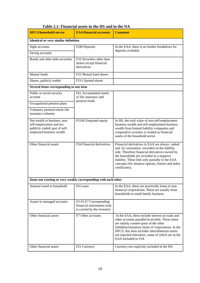
Table 2.1 shows the linkage between the financial assets in the HS/HFCS and the NA/EAA. For some asset types there is a direct linkage. Deposits, bonds and other debt securities, mutual funds and publicly traded shares are included in both sources with identical or very similar definitions. These items cover roughly 30% of all assets and 65 % of financial assets in the NA.

In the HS deposits are separated into sight and savings accounts, while the EAA does not distinguish different kinds of deposits. The HS sight accounts are equivalent to transferable deposits as defined by ESA95 (ESA95 5.42-5.45, ECB, 2010). The HS target variable on savings accounts covers non-transferable savings and time deposits and certificates of deposit.

The HS concept of bonds and other debt securities corresponds to securities other than shares excluding financial derivatives in the NA. In the NA, securities other than shares excluding financial derivatives can additionally be divided to long- and short-term securities. The HS concept of mutual funds corresponds to the mutual fund shares in the EAA (ESA95, 5.09). In the HS this item can be disaggregated into mutual funds investing predominantly in money market instruments, bonds and shares. The concept of publicly traded shares in the HS covers shares owned by households which are publicly traded in a stock exchange. This corresponds to the concept of quoted shares in the NA.

For other types of financial assets, either the item does not exist in the HS or there are several items in the HS corresponding to one item in NA or the item in HS does not even theoretically fully correspond to the asset in NA. These kinds of cases are briefly explained in the column “comment”. A more detailed description on the conceptual differences between HFCS and EAA has been provided by Kavonius and Törmälehto (2010).

The concept of managed accounts does not exist in the NA. Managed accounts are typically arrangements where a household trusts e.g. an investment company to manage the household’s investments. In the NA, the essential criterion is based on the legal ownership. In managed accounts the money is typically invested by the investment bank in the name of the investor, who only pays a service fee to the investment bank. The investor (household) is also the owner of the corresponding instruments.

The money owed to the household is included as an asset in both statistics, in the case of NA in loans on the asset rather than liability side. However, loans between the households are recorded in the HS, but not in the NA.

9 

In the EAA, financial derivatives are financial assets based on or derived from a different underlying instrument and financial derivatives owned by households are recorded as a negative liability. In the HS, the variable on any other financial assets should cover also financial derivatives such as options, futures or index certificates, among other assets not included elsewhere.

In the EAA, asset category “other accounts” is a similar type of residual category as “any other financial assets” in the HS, albeit with different content. It is included mainly for accounting reasons. In the case of the household sector, these are mainly interest accruals.

10 

Table 2.1: Financial assets in the HS and in the NA

HFCS/household survey EAA/financial accounts Comment

Identical or very similar definition

Sight accounts F2M Deposits In the EAA, there is no further breakdown for deposits available.

Saving accounts

Bonds and other debt securities F33 Securities other than shares except financial derivatives

 

Mutual funds F52 Mutual fund shares  

Shares, publicly traded F511 Quoted shares  

Several items corresponding to one item

Public or social security account

F61 Accumulated assets of life insurance and pension funds

 

Occupational pension plans

Voluntary pension/whole life insurance schemes

Net wealth in business, non- self-employment and not publicly traded; part of self- employed business wealth

F51M Unquoted equity In HS, the total value of non-self-employment business wealth and self-employment business wealth from limited liability companies and cooperative societies is treated as financial assets of the household sector.

Other financial assets F34 Financial derivatives Financial derivatives in EAA are always netted and by convention recorded on the liability side. Therefore financial derivatives owned by the households are recorded as a negative liability. These link only partially to the EAA concepts (for instance options, futures and index certificates).

Items not existing or very weakly corresponding with each other

Amount owed to household F4 Loans In the EAA, these are practically loans to non- financial corporations. These are usually from households to small family business.

Assets in managed accounts F2-F5,F7 Corresponding financial instruments (risk is carried by the investor)

 

Other financial assets F7 Other accounts In the EAA, these include interest accruals and other accounts payable/receivable. These items are mainly counter-parts of the other liabilities/transitory items of corporations. In the HFCS, this item includes miscellaneous assets not reported elsewhere, some of which are in the EAA included in F34.

Other financial assets F21 Currency Currency not explicitly included in the HS.

11 

 

Pension wealth is a major component of household wealth. The HS aims at measuring current termination value (“accrued-to-date liability”) of pension and whole life insurance assets. Entitlements to non-life insurance, including term life insurance, are not considered as household wealth. The HS target variables on pension wealth are broken down into public pension plans, public or social security account with account balance, occupational pension plans, and voluntary non-occupational pension/whole life insurance schemes, this breakdown being in line with the National Accounts classification (see: ECB, 2008, for details).

In the NA, the concept of insurance technical reserves may be interpreted as the functional equivalent of the HS pensions and whole life insurance variables. It covers the accumulated claims vis-à-vis life insurance and pension funds and the prepayment of insurance payments. The treatment of pension depends in the SNA93/SNA2008 on the type of pension plan. The current system includes defined contribution pension plans and individual defined benefit plans.

To some extent, pension wealth is different from other wealth components as it by and large is not liquid before old-age and cannot be bequeathed8. Besides, the measurement of pension wealth in household surveys is highly complicated and prone to measurement errors. The difficulty of collecting data on pension wealth from households has been fully recognised and the data on pensions from the first wave of survey are best viewed as experimental.

Unquoted equity in the NA consist of all transactions in unquoted shares which represent property rights on limited liability corporations and share their net assets in the event of liquidation. Other equity is the equity of incorporated partnerships, limited companies and quasi-corporations whose partners or owners are not shareholders (ESA95 5.90 and 5.95). The value of unquoted shares and other equity is not a separate asset type in the HS. It is covered under private wealth in businesses not publicly traded, including both participations in self-employment businesses (when at least one member of the household works in the business) and other passive investments in businesses in which household members are just silent partners. The self-employment concept is defined as net of liabilities rather than gross, in contrast to non-corporate business equity of investors and sleeping partners and other asset types.

The treatment of the items related to the HS concept “private business wealth” 9

in the NA depends on the type of enterprise. The wealth items of an enterprise can be recorded to the balance sheets of households or of financial or non-financial corporations. Furthermore, for some enterprise types other equity or unquoted shares that are recorded in the liability side of enterprises’ balance sheets are recorded as assets of the household sector. In HS, investments in non-self-employment private business wealth are classified as financial wealth, while self-employment business assets are classified as real wealth. However, the legal form of the self-employment enterprise is collected and this information is used to break down self-employment business wealth between real and financial assets of the household sector, to better match the NA definition. In this analysis we classify self-employment limited liability

 

     

8 At least this is the case for most public pension schemes, private and occupational pension wealth can often be liquidised before old age. 9 Business wealth in the HS includes also properties used for business purposes. This item is clearly not included in financial wealth of NA and is included in real wealth in this paper.

12 

companies and cooperative societies as financial wealth and sole proprietorships and partnerships as real wealth.10

The measurement of business wealth will, however, result in differences between the two sources because of the difficulties to divide the survey definition of “business wealth” to different sectors of NA. Also, self-employment business wealth is a net concept in the HS. It should be noted that these differences do not affect the concept of net wealth, only its components.

 

2.2Liabilities 

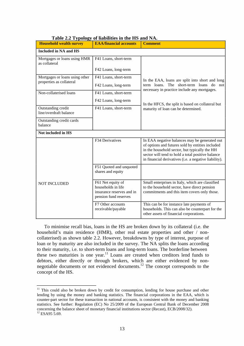
Table 2.2 shows the linkage between liabilities in the HS/HFCS and NA/EAA. In the HS, liabilities consist of mortgages and loans, credit lines, overdraft balances, and outstanding credit card balances. The NA covers also these balance sheet items and on top of this some other small balance sheet items which are either related to accounting conventions or in some country-specific cases.

 

                                              

10 These figures exist for Italy and the Netherlands, with 29 and 28% respectively of the values of self- employment businesses classified as financial wealth. For Finland we use the average of these shares.

13 

 

Table 2.2 Typology of liabilities in the HS and NA. Household wealth survey EAA/financial accounts Comment

Included in NA and HS

Mortgages or loans using HMR as collateral

F41 Loans, short-term  

 F42 Loans, long-term

    In the EAA, loans are split into short and long term loans. The short-term loans do not necessary in practice include any mortgages.  

 In the HFCS, the split is based on collateral but maturity of loan can be determined.

Mortgages or loans using other properties as collateral

F41 Loans, short-term  

F42 Loans, long-term

Non-collaterised loans F41 Loans, short-term  

F42 Loans, long-term

Outstanding credit line/overdraft balance

F41 Loans, short-term

Outstanding credit cards balance

Not included in HS

         

 NOT INCLUDED

F34 Derivatives In EAA negative balances may be generated out of options and futures sold by entities included in the household sector, but typically the HH sector will tend to hold a total positive balance in financial derivatives (i.e. a negative liability).

F51 Quoted and unquoted shares and equity

 

F61 Net equity of households in life insurance reserves and in pension fund reserves

Small enterprises in Italy, which are classified to the household sector, have direct pension commitments and this item covers only those.

F7 Other accounts receivable/payable

This can be for instance late payments of households. This can also be counterpart for the other assets of financial corporations.

 

To minimise recall bias, loans in the HS are broken down by its collateral (i.e. the household’s main residence (HMR), other real estate properties and other / non- collaterised) as shown table 2.2. However, breakdowns by type of interest, purpose of loan or by maturity are also included in the survey. The NA splits the loans according to their maturity, i.e. to short-term loans and long-term loans. The borderline between these two maturities is one year.11 Loans are created when creditors lend funds to debtors, either directly or through brokers, which are either evidenced by non- negotiable documents or not evidenced documents.12 The concept corresponds to the concept of the HS.

   

11 This could also be broken down by credit for consumption, lending for house purchase and other lending by using the money and banking statistics. The financial corporations in the EAA, which is counter-part sector for these transaction in national accounts, is consistent with the money and banking statistics. See further: Regulation (EC) No 25/2009 of the European Central Bank of December 2008 concerning the balance sheet of monetary financial institutions sector (Recast), ECB/2008/32). 12 ESA95 5.69.

14 

2.3Income 

Income in the HS/HFCS is collected for ten different concepts and additionally, for a mop-up category “Other income received”. Part of the income components are collected at the personal level from all household members aged 16 or older, others are collected at the household level only. The collection of personal level income from all household members is essential in order to capture total household income (Van den Heede et al. 2012). However, some income items, such as public transfers and rental income, cannot necessarily be attributed to individual persons, but can be collected at the household level only. Only gross income variables are compulsory, but for some countries, including Finland and Italy, disposable income can also be constructed.

In the NA/EAA, i.e. also in the sector accounts, income concept covers all the income received/paid in the accounting period. The income concept is based on the European System of Accounts 1995 (ESA95). The most common concept used in the context of households in national accounting is disposable income. However, disposable income as well as other balancing items is calculated from its components. In this paper we build from the individual transactions an income concept which is as near as possible to the concept applied in the HS.

In the HS, employee income is the sum of remuneration received from an employer in cash. This includes some near-cash components, such as stock options. This concept corresponds to wages and salaries in the NA. Wages and salaries are the remuneration paid in cash or in kind for work done during the accounting period. Employee stock options are not covered by the wages and salaries as realised and unrealised holding gains, which employee stock options are by nature, are classified as other changes, i.e. price changes, of stocks.13 This component does not cover social contributions payable by the employer in neither source.

Income from self-employment is the net operating profit or loss that a self- employed person makes out of his or her unincorporated enterprise. This is defined as gross revenue (including subsidies) minus operating costs, wages and salaries paid to employees, including social contributions, taxes paid on production and imports, interest paid on business loans, and depreciation of fixed assets. The business of a self-employed person may make a loss which is regarded as negative income. In NA for income from quasi-corporations would be theoretically possible to estimate entrepreneurial income. Unincorporated enterprises are included in the households sector and those refer to enterprises which cannot be separated from a household. This kind of business do not necessarily have own book-keeping and household wealth is at risk if the enterprise goes bankrupt.

                

13 See more on the employee stock options and the income concept of NA: Kavonius 2006.

15 

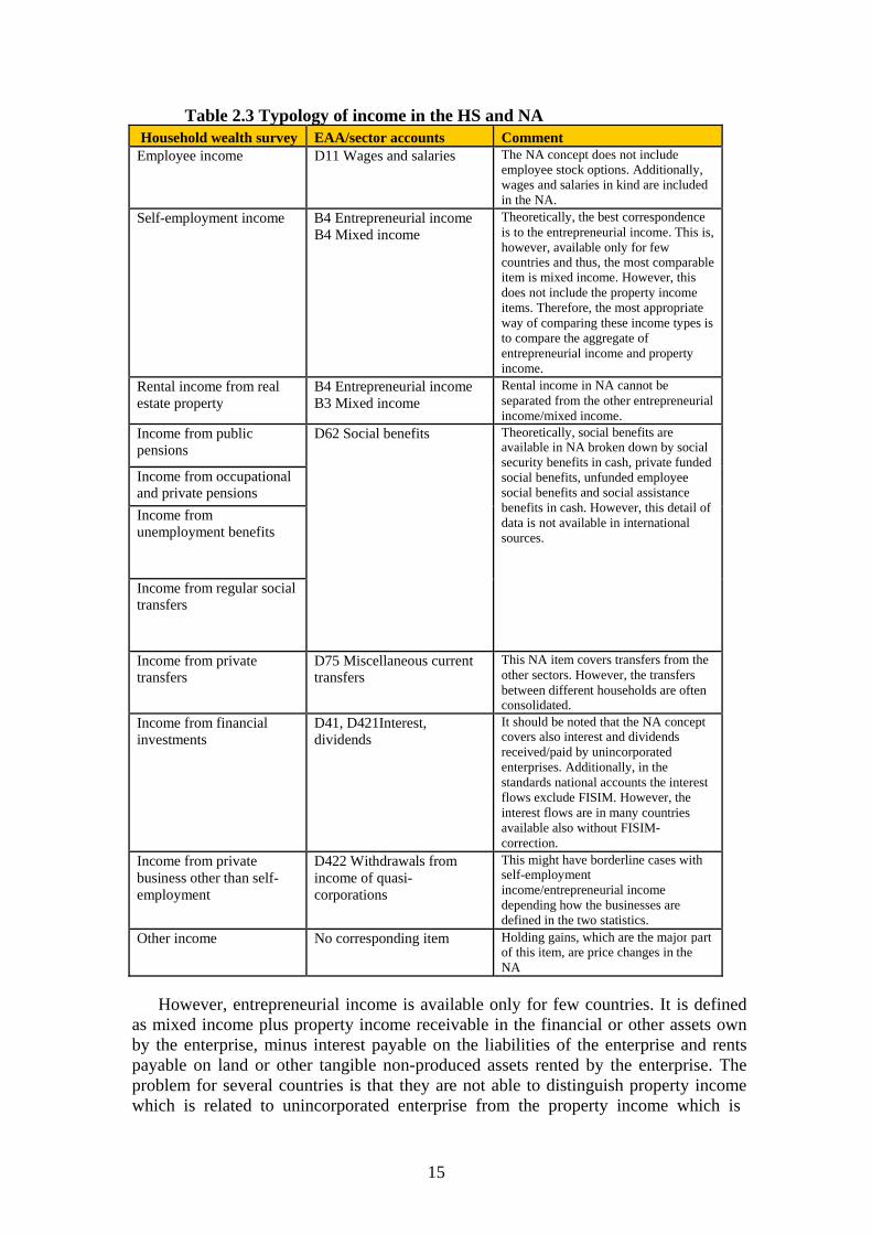
Table 2.3 Typology of income in the HS and NA Household wealth survey EAA/sector accounts Comment

Employee income D11 Wages and salaries The NA concept does not include employee stock options. Additionally, wages and salaries in kind are included in the NA.

Self-employment income B4 Entrepreneurial income B4 Mixed income

Theoretically, the best correspondence is to the entrepreneurial income. This is, however, available only for few countries and thus, the most comparable item is mixed income. However, this does not include the property income items. Therefore, the most appropriate way of comparing these income types is to compare the aggregate of entrepreneurial income and property income.

Rental income from real estate property

B4 Entrepreneurial income B3 Mixed income

Rental income in NA cannot be separated from the other entrepreneurial income/mixed income.

Income from public pensions

D62 Social benefits Theoretically, social benefits are available in NA broken down by social security benefits in cash, private funded social benefits, unfunded employee social benefits and social assistance benefits in cash. However, this detail of data is not available in international sources.

Income from occupational and private pensions

Income from unemployment benefits

Income from regular social transfers

Income from private transfers

D75 Miscellaneous current transfers

This NA item covers transfers from the other sectors. However, the transfers between different households are often consolidated.

Income from financial investments

D41, D421Interest, dividends

It should be noted that the NA concept covers also interest and dividends received/paid by unincorporated enterprises. Additionally, in the standards national accounts the interest flows exclude FISIM. However, the interest flows are in many countries available also without FISIM- correction.

Income from private business other than self- employment

D422 Withdrawals from income of quasi- corporations

This might have borderline cases with self-employment income/entrepreneurial income depending how the businesses are defined in the two statistics.

Other income No corresponding item Holding gains, which are the major part of this item, are price changes in the NA

 

However, entrepreneurial income is available only for few countries. It is defined as mixed income plus property income receivable in the financial or other assets own by the enterprise, minus interest payable on the liabilities of the enterprise and rents payable on land or other tangible non-produced assets rented by the enterprise. The problem for several countries is that they are not able to distinguish property income which is related to unincorporated enterprise from the property income which is

16 

related to households overall activities. For the countries discussed in this paper only for Finland entrepreneurial income and mixed income is available. For Italy gross mixed income is available and the net was estimated by breaking down consumption fixed capital by the distribution between gross operating surplus and mixed income. In the case of the Netherlands it is not possible even to split operating surplus and mixed income.

Income from private business other than self-employment refers to the amount of profits from capital investment in unincorporated and incorporated not publicly traded private businesses received less expenses incurred. This roughly corresponds to the withdrawals from the income of quasi-corporations. These are in practice withdrawals from quasi-corporations or incorporated partnerships, i.e. corporations which are not allocated in household sector. The practical problem in this case as well in the case of entrepreneurial income is the delineation of the household sector, that is to distinguish which corporations are unincorporated, incorporated or quasi- corporations and whether this borderline is consistent between the two statistics.

Rental income from real estate property includes income received from renting a property or land, after deducting costs such as mortgage interest repayments, minor repairs, maintenance, insurance and other charges. If renting of the property is part of an unincorporated business, the income should be part of the self-employment income. In the case of NA, rental income is mixed income of households, i.e. the rental business is classified as a business of unincorporated enterprise. The rental income of the HS is equivalent to the concept of entrepreneurial income (from rental activities) in the NA but as indicated earlier, this cannot be calculated for all the countries. Additionally, it is not possible to separate in NA rental income from the other entrepreneurial income. Therefore, the most correct way to compare these items is to aggregate rents from land items and mixed income or entrepreneurial income items and to compare this aggregated item.

Income from financial investments includes interest received from assets such as bank accounts, certificates of deposit, bonds, publicly traded shares etc. less expenses incurred, plus dividends received. This item corresponds to interest and dividends in the national accounts. Additionally, NA classify withdrawals from quasi-corporations, property income attributed to insurance policy holders and rents from land. The property income attributed to insurance policy holders is not covered by the HS-concept. As mentioned earlier, withdrawals correspond to the income from private business other than self-employment although many countries do not report this item.

In NA, the concept social benefits other than social transfers in kind includes all items classified as (public) transfer income in household surveys. According the SNA93 and ESA95 there is further detail for social transfers where they are broken down by private funded benefits and unfunded employee benefits. This detail, however, is not transmitted by countries and therefore, the comparison must be done at the level of social benefits.

There are three items for public transfers in the HS. Income from public pensions includes old age pensions, anticipated old age pensions (periodic payments intended to maintain the income of beneficiaries who retire before the standard age), partial retirement pensions, survivor’s pension and disability pension. Unemployment income includes full and partial unemployment benefits, benefits for early retirement for labour market reasons, vocational training allowances and mobility and resettlement payments by social security funds or public agencies, and other unemployment financial assistance, particularly payments to the long-term

17 

unemployed. Income from regular social transfers includes any regular transfers to individuals, families or households from social security or other governmental agencies (excluding items reported under pensions or unemployment benefits) such as illness subsidies, maternity leave, family protection, child benefits, student grants and other educational assistance, tax credits etc.

Pensions received from occupational and private pension plans are collected as a separate category. In the national accounts this item is covered by insurance technical reserves. The pensions received are classified as social transfers. Income from private transfers refers to any regular transfers from private entities or other households, for example alimony and child support. The recording of these items depend on who is paying these transfers. In the all of the cases, these are classified as current transfers but these are additionally broken down by payer sector. In the case of transfers paid by the other households, the manuals recognise transfers paid by the other households but in practice several countries do not have those figures. NA treat households as a joint sector, at the aggregate level countries produce in a sense consolidated figures and the transfers “cancel out” within the sector.

The mop-up category other income received in HS refers to any income source not classified earlier. This might include such items as capital gains or losses from the sale of assets, severance and termination payments, lump sum payments upon retirement or premature withdrawals from private pension schemes, prize winnings or insurance settlements.

 

3Potentialdifferencesinthetwostatistics 

There are many reasons why sample survey estimates and corresponding NA totals might differ. In this paper, we classify the differences to following three groups: (1.) Macro versus micro point of view; (2.) Errors in estimation: population coverage and sampling; and finally, (3.) Errors in measurement: timing and differences in data collection methods. This list might not be comprehensive but it covers the most of the differences between these two sources.

 

3.1Macroversusmicropointofview 

The different aspects of the statistics might cause differences from three points of view: first from the conceptual point of view, i.e. some concepts do not necessarily make sense at balanced macro level system as they do at micro level. Second, the valuation of some instruments might be easier at macro than at micro level. Finally, the balancing framework might lead to the situation that some data is estimated by using accounting rules or counterpart information.

Concerning the conceptual issues, the micro survey focuses only on one individual household which forces one to define the concepts from the household point of view. In the NA, the concepts are defined at total economy level and are also counter-parted to the other sectors. This might lead to conceptual differences. On the wealth side, business wealth can be mentioned as an example. As explained earlier, business wealth is one accumulated stock of wealth from the household point of view, as in the NA the different parts of business wealth are distributed to different instruments of the NA.

The different aspects affect the valuation of different wealth components. The non-financial assets, i.e. predominantly housing wealth, are relatively easy to estimate at the micro level. The source data of total financial wealth are, however, more

18 

complete and reliable than in micro statistics and therefore, the financial flows at macro level are more reliable than in the surveys. Consequently, in wealth surveys the share of non-financial assets in total wealth has been recorded as significantly higher compared to the NA (74 – 88 % in the three countries analysed in this paper).

The data collection and the balancing framework, i.e. the process which aims to reach this consistency in the accounting system, have a twofold effect on the accounts. On the one hand, the accounting system forces to cross-check different data sources and gets them as comparable and consistent as possible before the balancing.14 From this point of view, it can be argued that NA data at total household levels provide more reliable estimates than data retrieved from an individual data source. On the other hand, as in this balancing process the inconsistencies or discrepancies are distributed through the accounts according to relative weights of the items, it is possible that errors in measurement from other sources or sectors balance out and eventually contribute to “correct the data” to a certain extent (if one relies on simplified processes or uninformed integrators). Moreover, it should be emphasised that these kinds of balancing adjustments are typically very small. Typically, if the size of total balancing adjustment is known, it can be considered as an error margin for the estimations.

NA may need to allow some bias in the household sector to satisfy the balancing constraints, i.e. the ultimate aim is not to minimize bias in the household sector; rather there is the dual objective to minimize bias in the estimates for the economy as a whole and to minimize statistical discrepancies within the system. The latter may result in bias within sectors, for instance, certain economic transactions for the household sector may be derived as residual, by subtracting from the estimated total the estimates of other institutional sectors.

NA are typically based on other statistical sources and the validation of the used sources. The possible other errors are inherited from source statistics. The errors in estimation can be of course caused by two reasons: either statistics used in the NA estimation are compiled according to a different methodology than the NA (and this is not corrected when they are incorporated to the NA) or there is a measurement error in the source statistics.

 

3.2Errorsinestimation:populationcoverageandsampling 

The quality of the estimates based on a household sample survey may be thought of in terms of errors in estimation and errors in measurement. Errors in measurement occur when the value that is recorded for a household in the sample departs from the actual true value for the household. Errors in estimation are errors in the extrapolation from the households enumerated in the survey to the entire population of private households for which estimates are required. Item non-

  

14 The national household sector balance sheets are generally compiled using counterpart information and residual estimations as there are not many direct sources concerning households available. The accounting data are typically balanced at the level of the whole economy. In the balancing three dimensions can be found: First, total financial assets equal total financial liabilities for each financial balance sheet category, when summed over all institutional sectors and rest of the world. This is so called horizontal consistency. Second, the change in financial balance sheet for each balance sheet category equal to the sum of the financial transactions and other changes, like revaluation of assets. This is called stock-flow consistency. Similarly, total non-financial assets equal to the sum of non- financial transaction and consumption of fixed capital. Third, for each sector and rest of the world, the balance of all current and capital transactions should be equal to the balance of financial transactions and this is called vertical consistency.

19 

response can be classified as a mixed category between measurement and estimation error (Verma and Betti, 2010).

The first group of estimation errors are coverage errors. This arises if the target population is different from the sampling frame or if all units in the frame do not have a random non-zero probability of being selected. In the wealth surveys analysed in this paper probability sampling is used, meaning that the second case would never occur.

Persons living collective households and institutions are generally excluded from the target population of household surveys as these included in the NA. The share of persons living in collective households and institutions vary from country to country. Based on the 2001 population census in Finland 1.9 per cent, in Italy 0.7 per cent and in the Netherlands 1.4 per cent of the population are living in collective households and institutions (Eurostat) as also indicated in table 3.2. Unfortunately, there is no information what share of assets and liabilities can be attributed to this group; it seems that the population share is the only available proxy.

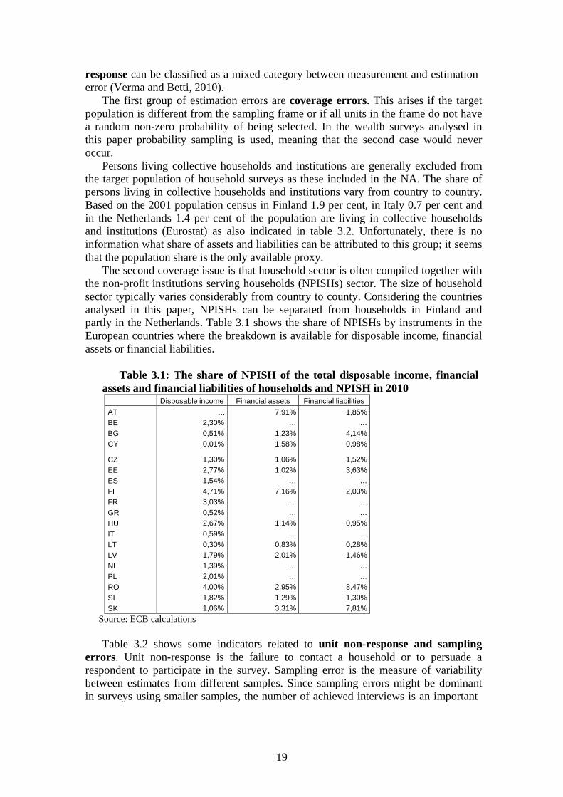
The second coverage issue is that household sector is often compiled together with the non-profit institutions serving households (NPISHs) sector. The size of household sector typically varies considerably from country to county. Considering the countries analysed in this paper, NPISHs can be separated from households in Finland and partly in the Netherlands. Table 3.1 shows the share of NPISHs by instruments in the European countries where the breakdown is available for disposable income, financial assets or financial liabilities.  

Table 3.1: The share of NPISH of the total disposable income, financial assets and financial liabilities of households and NPISH in 2010   Disposable income Financial assets Financial liabilities

AT

BE

BG

CY  

CZ

EE

ES

FI

FR

GR

HU

IT

LT

LV

NL

PL

RO

SI

SK

…

2,30%

0,51%

0,01%  

1,30%

2,77%

1,54%

4,71%

3,03%

0,52%

2,67%

0,59%

0,30%

1,79%

1,39%

2,01%

4,00%

1,82%

1,06%

7,91%

…

1,23%

1,58% 

1,06%

1,02%

…

7,16%

…

…

1,14%

…

0,83%

2,01%

…

…

2,95%

1,29%

3,31%

1,85%

…

4,14%

0,98% 

1,52%

3,63%

…

2,03%

…

…

0,95%

…

0,28%

1,46%

…

…

8,47%

1,30%

7,81%

Source: ECB calculations  

Table 3.2 shows some indicators related to unit non-response and sampling errors. Unit non-response is the failure to contact a household or to persuade a respondent to participate in the survey. Sampling error is the measure of variability between estimates from different samples. Since sampling errors might be dominant in surveys using smaller samples, the number of achieved interviews is an important

20 

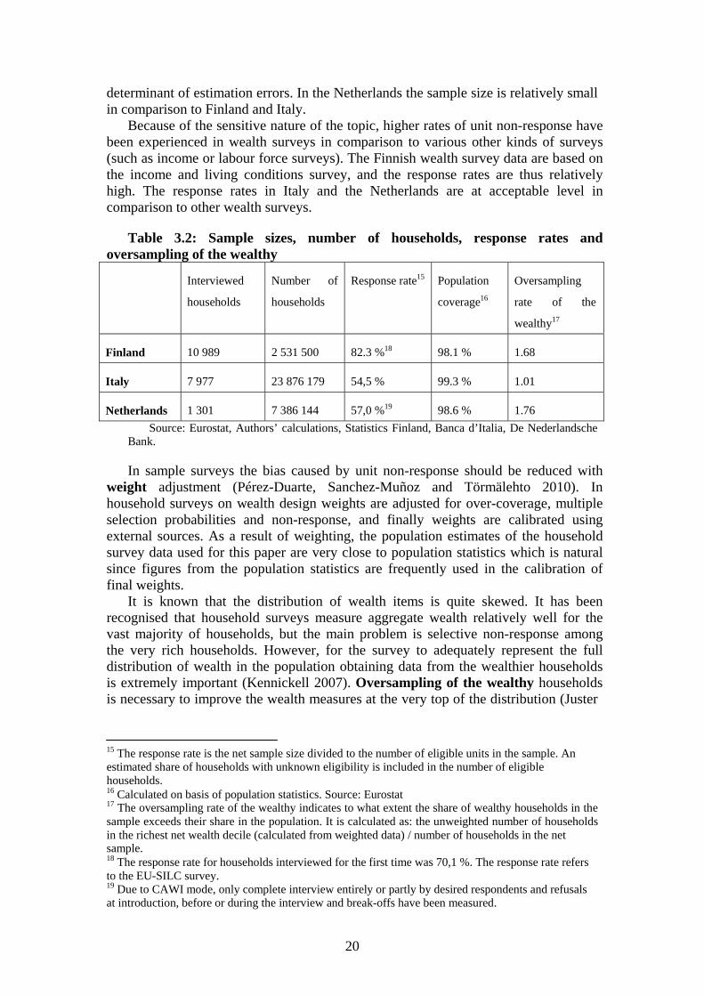
determinant of estimation errors. In the Netherlands the sample size is relatively small in comparison to Finland and Italy.

Because of the sensitive nature of the topic, higher rates of unit non-response have been experienced in wealth surveys in comparison to various other kinds of surveys (such as income or labour force surveys). The Finnish wealth survey data are based on the income and living conditions survey, and the response rates are thus relatively high. The response rates in Italy and the Netherlands are at acceptable level in comparison to other wealth surveys.

 Table 3.2: Sample sizes, number of households, response rates and

oversampling of the wealthy    

Interviewed

households

 Number of

households

Response rate15 Population

coverage16

 Oversampling

rate of the

wealthy17

 Finland

 10 989

 2 531 500 82.3 %18

98.1 %  

1.68  

Italy  

7 977  

23 876 179 54,5 % 99.3 %  

1.01  

Netherlands  

1 301  

7 386 144 57,0 %19 98.6 %

 1.76

Source: Eurostat, Authors’ calculations, Statistics Finland, Banca d’Italia, De Nederlandsche Bank.

 In sample surveys the bias caused by unit non-response should be reduced with

weight adjustment (Pérez-Duarte, Sanchez-Muñoz and Törmälehto 2010). In household surveys on wealth design weights are adjusted for over-coverage, multiple selection probabilities and non-response, and finally weights are calibrated using external sources. As a result of weighting, the population estimates of the household survey data used for this paper are very close to population statistics which is natural since figures from the population statistics are frequently used in the calibration of final weights.

It is known that the distribution of wealth items is quite skewed. It has been recognised that household surveys measure aggregate wealth relatively well for the vast majority of households, but the main problem is selective non-response among the very rich households. However, for the survey to adequately represent the full distribution of wealth in the population obtaining data from the wealthier households is extremely important (Kennickell 2007). Oversampling of the wealthy households is necessary to improve the wealth measures at the very top of the distribution (Juster

   

15 The response rate is the net sample size divided to the number of eligible units in the sample. An estimated share of households with unknown eligibility is included in the number of eligible households. 16 Calculated on basis of population statistics. Source: Eurostat 17 The oversampling rate of the wealthy indicates to what extent the share of wealthy households in the sample exceeds their share in the population. It is calculated as: the unweighted number of households in the richest net wealth decile (calculated from weighted data) / number of households in the net sample. 18 The response rate for households interviewed for the first time was 70,1 %. The response rate refers to the EU-SILC survey. 19 Due to CAWI mode, only complete interview entirely or partly by desired respondents and refusals at introduction, before or during the interview and break-offs have been measured.

21 

et al. 1999). This will lead to both a better coverage of the wealthiest households and correct for the selective unit non-response. .

Determining wealthy households ex-ante requires feasible external information on households. In Finland income register data is used to select more units to the gross sample from strata having higher income levels. In Italy or the Netherlands no such registers are available in central banks or survey companies, and wealthy households are not systematically oversampled. However, the share of wealthy households in the Dutch net sample is even higher than in Finland.

 

3.3Errorsinmeasurementduetoitemnon‐response,timinganddifferencesindatacollectionmethods

 Item non-response occurs when the respondent is not able or is unwilling to

provide an answer to a specific question. Given the difficulties in the concepts of some balance sheet variables, a non-ignorable degree of item non-response can be expected in wealth surveys. Of the three data sets used in this paper, item non- response is a noteworthy issue only in the Netherlands, where multiple imputation methodology (see Rubin 1987) was applied to correct for partially non-ignorable degree of item non-response. For Finland – having all balance sheet or income variables collected from registers – item non-response is naturally not relevant. In the Italian data item non-response is very low due to the incentive structure for interviewers. Later, when euro area data are available, imputation becomes a more relevant issue, and specific emphasis should be put on the analysis of multiple imputation, used in most euro area countries.

The scope for measurement errors due to differences in the definition of variables was described in chapter two. Another basic conceptual difference between HS and NA is timing. The three countries analysed in this paper use the last day of the previous calendar year (2008 in Italy, 2009 in Finland and the Netherlands) as a reference period for stocks. For income items all three countries use probably the most common approach, the entire calendar year preceding the fieldwork period (2008 Italy, 2009 Finland and the Netherlands), as a reference period. In the annual NA data used in this analysis the reference date of the stock is the last day of the year. While reference periods do not cause any comparability problems for country comparisons, the issue becomes more problematic when figures are constructed for the euro area, with various countries using different reference periods.

Survey design literature and further empirical evidence show that the survey mode is an important determinant of measurement error. It has been argued that Computer Assisted Personal Interview is the most reliable method for data collection. The use of a computer allows a smooth and error-free administration of the routing of the questions, the application of consistency checks during the interview and the automatic storage of the data. Personal contact with respondents is needed to persuade respondents to participate in the survey and complete the questionnaire by building up trust vis-à-vis respondents and to provide additional assistance and information during the interview if required (ECB 2008).

In Italy the main data collection method was CAPI, the share of which was 80 % of achieved interviews. The rest of the interviews were conducted via Paper Assisted Personal Interviews. The wealth survey data from the Netherlands is collected via Computer Assisted Web Survey (CAWI). The balance sheet variables in Finland are collected from registers, either directly or with the use of estimation methods. All register data available in Statistics Finland can be linked to the demographic

22 

information of the EU-SILC sample of with personal ID’s. Consequently, problems of underreporting can be avoided with this method if the quality and coverage of the registers is very good. On the other hand, the net sample consists of households having responded to a CATI interview. Evidence has shown that telephone interviews lead to a higher unit non-response at the tails of the distribution (Fessler et al. 2012). Also, some definitional issues may be involved the use of register data.

Register data is used in Finland directly to construct variables for income, debt, mutual funds, bonds and publicly traded shares. The definitions of register variables are identical or very similar to the survey variables. The coverage of individual level income data compared to the requirements of the HFCS is very good. Few items that are not available in registers, such as private transfers and interest payments, are collected in the EU-SILC survey. Income data on public transfers available in registers is more detailed than the survey requirements, which will decrease the possible recall bias caused in the survey data20. Most liabilities items can also be measured accurately from registers. Estimation methods are used for unlisted shares, deposits and real assets. These methods include some uncertainties and possible comparability issues.

 

                                          

20 In the HFCS there are three questions on public transfers: public pension income, unemployment income and other public transfers. Administrative sources used in the Finnish HFCS include very detailed information on several types of public transfers received.

23 

4Thelinkagebetweenthetwostatisticsandreasonsfordiscrepancies

 

 

The purpose of this section is to discuss the results, i.e. the comparability of the two statistics and also to try to quantify what the sources of the differences are. Finally, the results concerning the NA broken down by the HS are presented and the validity of these results is discussed. While the comparison of definitions was based on euro area data sources (EAA, HFCS), the data comparison is made using national sources both at the micro and macro level. Although the attempt is to benchmark national sources to the corresponding euro area frameworks, the conversion of national level data to harmonised data might cause discrepancies not analysed further in this paper.

 

4.1Assetsandliabilities 

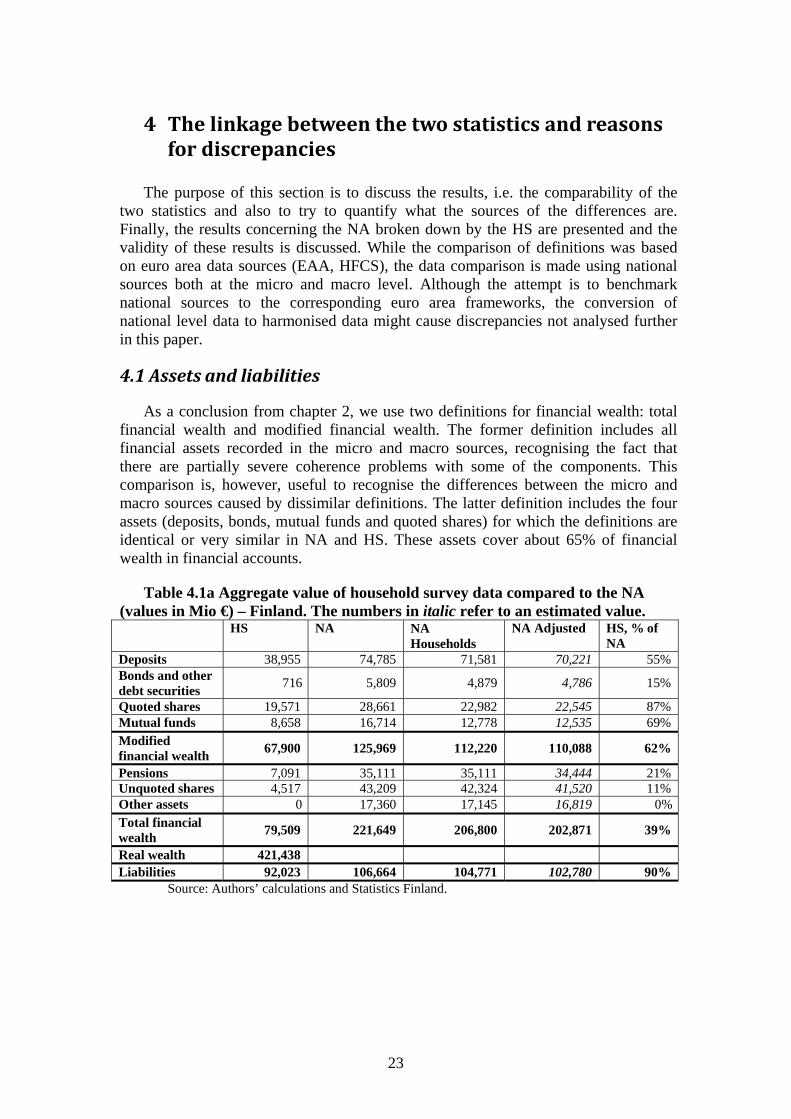
As a conclusion from chapter 2, we use two definitions for financial wealth: total financial wealth and modified financial wealth. The former definition includes all financial assets recorded in the micro and macro sources, recognising the fact that there are partially severe coherence problems with some of the components. This comparison is, however, useful to recognise the differences between the micro and macro sources caused by dissimilar definitions. The latter definition includes the four assets (deposits, bonds, mutual funds and quoted shares) for which the definitions are identical or very similar in NA and HS. These assets cover about 65% of financial wealth in financial accounts.

 Table 4.1a Aggregate value of household survey data compared to the NA

(values in Mio €) – Finland. The numbers in italic refer to an estimated value.   HS NA NA

HouseholdsNA Adjusted HS, % of

NA Deposits 38,955 74,785 71,581 70,221 55% Bonds and other debt securities

 

716  

5,809 4,879 4,786  

15%

Quoted shares 19,571 28,661 22,982 22,545 87% Mutual funds 8,658 16,714 12,778 12,535 69% Modified financial wealth

 

67,900  

125,969 112,220 110,088  

62%

Pensions 7,091 35,111 35,111 34,444 21%Unquoted shares 4,517 43,209 42,324 41,520 11% Other assets 0 17,360 17,145 16,819 0%Total financial wealth

 

79,509  

221,649 206,800 202,871  

39%

Real wealth 421,438    Liabilities 92,023 106,664 104,771 102,780 90%

Source: Authors’ calculations and Statistics Finland.

24 

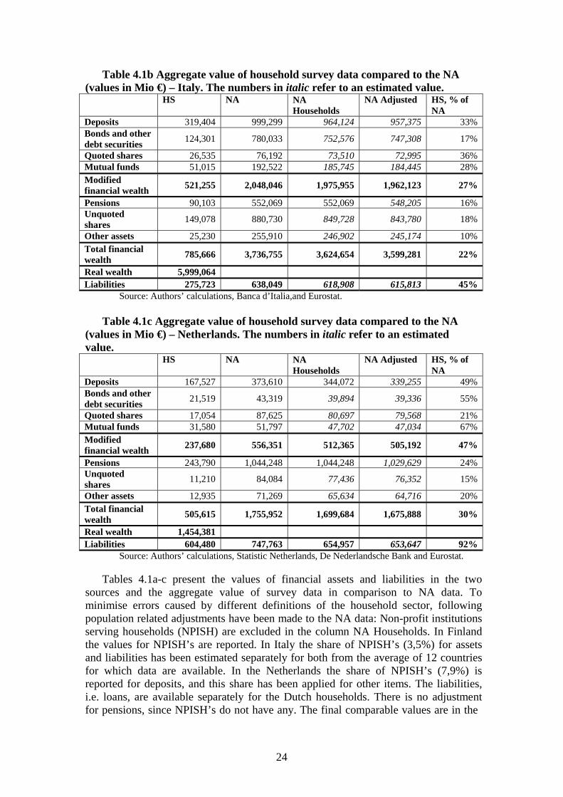
Table 4.1b Aggregate value of household survey data compared to the NA (values in Mio €) – Italy. The numbers in italic refer to an estimated value.

  HS NA NA Households

NA Adjusted HS, % of NA

Deposits 319,404 999,299 964,124 957,375 33% Bonds and other debt securities

 

124,301  

780,033 752,576 747,308  

17%

Quoted shares 26,535 76,192 73,510 72,995 36% Mutual funds 51,015 192,522 185,745 184,445 28% Modified financial wealth

 

521,255  

2,048,046 1,975,955 1,962,123  

27%

Pensions 90,103 552,069 552,069 548,205 16%Unquoted shares

 

149,078  

880,730 849,728 843,780  

18%

Other assets 25,230 255,910 246,902 245,174 10% Total financial wealth

 

785,666  

3,736,755 3,624,654 3,599,281  

22%

Real wealth 5,999,064    Liabilities 275,723 638,049 618,908 615,813 45%

Source: Authors’ calculations, Banca d’Italia,and Eurostat.  

Table 4.1c Aggregate value of household survey data compared to the NA (values in Mio €) – Netherlands. The numbers in italic refer to an estimated value.

  HS NA NA Households

NA Adjusted HS, % of NA

Deposits 167,527 373,610 344,072 339,255 49% Bonds and other debt securities

 

21,519  

43,319 39,894 39,336  

55%

Quoted shares 17,054 87,625 80,697 79,568 21% Mutual funds 31,580 51,797 47,702 47,034 67% Modified financial wealth

 

237,680  

556,351 512,365 505,192  

47%

Pensions 243,790 1,044,248 1,044,248 1,029,629 24%Unquoted shares

 

11,210  

84,084 77,436 76,352  

15%

Other assets 12,935 71,269 65,634 64,716 20% Total financial wealth

 

505,615  

1,755,952 1,699,684 1,675,888  

30%

Real wealth 1,454,381    Liabilities 604,480 747,763 654,957 653,647 92%

Source: Authors’ calculations, Statistic Netherlands, De Nederlandsche Bank and Eurostat.  

Tables 4.1a-c present the values of financial assets and liabilities in the two sources and the aggregate value of survey data in comparison to NA data. To minimise errors caused by different definitions of the household sector, following population related adjustments have been made to the NA data: Non-profit institutions serving households (NPISH) are excluded in the column NA Households. In Finland the values for NPISH’s are reported. In Italy the share of NPISH’s (3,5%) for assets and liabilities has been estimated separately for both from the average of 12 countries for which data are available. In the Netherlands the share of NPISH’s (7,9%) is reported for deposits, and this share has been applied for other items. The liabilities, i.e. loans, are available separately for the Dutch households. There is no adjustment for pensions, since NPISH’s do not have any. The final comparable values are in the

25 

column NA Adjusted which is adjusted by population coverage figures presented in table 3.2.

The aggregate value of modified financial wealth in survey data compared to financial accounts data varies from 27% in Italy to 62% in Finland. The ratios seem quite low, but are not contradicting the problems in household level data collection on financial wealth that have been experienced earlier. There is quite significant variation in the ratios between HS and NA data both between various wealth items and between different countries. The fact that the aggregate values of remaining items in total financial wealth in HS data are very low compared to NA data highlights the comparability problems in these definitions.

Based on earlier chapters, population coverage, item non-response or timing does not seem to be a significant cause for the differences in the values of modified financial wealth. However, measurement errors at the household level, also related to the mode of data collection, and estimation errors related to the achieved sample size and sampling design deserve some attention.

Two possibilities of measurement errors at the household level should be distinguished: either a household reports a false value for an item, or a household having an item reports not having it. The problem with the analysis of survey measurement errors is that “true” values of households’ assets are rarely available. Therefore, very limited literature on the tendency of households to over- or under- report asset values in surveys exists. A comparison between survey data and administrative data with similar definitions in Sweden (Johansson and Klevmarken 2007) showed no evidence of systematic under-reporting of wealth items in surveys.

In Finland, values for quoted shares, bonds and mutual funds are constructed using register data that can be matched to the sample by personal identification codes. This should minimise the number of cases where information on having the item is completely missing. However, the valuation of the items is a potential source of measurement errors. Additionally, municipal and sovereign bonds are missing from the register data used in Finland. Deposits in Finland are estimated with statistical matching methodology. The use of these figures at the individual level is not recommended by the data producer but the aggregate value of HS deposits compared to NA data is at a comparatively reasonable level.

From the two countries that use survey data to collect asset values, the aggregate values of survey data in relation to NA data are higher in the Netherlands. This could be explained by the use of a web-panel. First of all, a high share of respondents consists of panel households having more experience in reporting the values of assets. Moreover, the distribution of respondents by certain characteristics has been observed to be different in web surveys compared to survey modes with interviewer involvement (Revilla 2010, Martin and Lynn 2011). Finally, while there are no experiences on this from mixed-mode surveys on wealth, a self-administered survey mode does not necessarily seem to have a negative impact on the collection of assets and other objectively measurable variables.

In addition to the survey mode, the main reasons behind the differences in aggregate values of HS data may be related to the sampling design and the ability to collect data efficiently from the wealthiest households. Since wealth is very unequally distributed, it is essential that data from the wealthiest part of the population are collected comprehensively and reliably to get valid data on aggregate wealth. This issue becomes even more relevant when comparing individual wealth components that are owned only by small fractions of the population.

26 

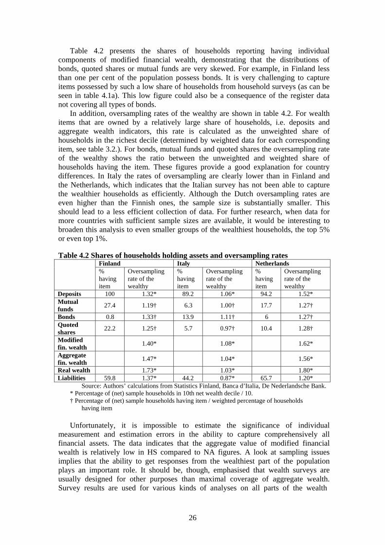
Table 4.2 presents the shares of households reporting having individual components of modified financial wealth, demonstrating that the distributions of bonds, quoted shares or mutual funds are very skewed. For example, in Finland less than one per cent of the population possess bonds. It is very challenging to capture items possessed by such a low share of households from household surveys (as can be seen in table 4.1a). This low figure could also be a consequence of the register data not covering all types of bonds.

In addition, oversampling rates of the wealthy are shown in table 4.2. For wealth items that are owned by a relatively large share of households, i.e. deposits and aggregate wealth indicators, this rate is calculated as the unweighted share of households in the richest decile (determined by weighted data for each corresponding item, see table 3.2.). For bonds, mutual funds and quoted shares the oversampling rate of the wealthy shows the ratio between the unweighted and weighted share of households having the item. These figures provide a good explanation for country differences. In Italy the rates of oversampling are clearly lower than in Finland and the Netherlands, which indicates that the Italian survey has not been able to capture the wealthier households as efficiently. Although the Dutch oversampling rates are even higher than the Finnish ones, the sample size is substantially smaller. This should lead to a less efficient collection of data. For further research, when data for more countries with sufficient sample sizes are available, it would be interesting to broaden this analysis to even smaller groups of the wealthiest households, the top 5% or even top 1%.

 Table 4.2 Shares of households holding assets and oversampling rates

  Finland Italy Netherlands % having item

Oversampling rate of the wealthy

% having item

Oversampling rate of the wealthy

% having item

Oversampling rate of the wealthy

Deposits 100 1.32* 89.2 1.06* 94.2 1.52* Mutual funds

 

27.4  

1.19† 6.3 1.00† 17.7  

1.27†

Bonds 0.8 1.33† 13.9 1.11† 6 1.27† Quoted shares

 

22.2  

1.25† 5.7 0.97† 10.4  

1.28†

Modified fin. wealth

  

1.40*   1.08*   

1.62*

Aggregate fin. wealth

  

1.47*   1.04*   

1.56*

Real wealth   1.73* 1.03* 1.80* Liabilities 59.8 1.37* 44.2 0.87* 65.7 1.20*

Source: Authors’ calculations from Statistics Finland, Banca d’Italia, De Nederlandsche Bank. * Percentage of (net) sample households in 10th net wealth decile / 10. † Percentage of (net) sample households having item / weighted percentage of households

having item  

Unfortunately, it is impossible to estimate the significance of individual measurement and estimation errors in the ability to capture comprehensively all financial assets. The data indicates that the aggregate value of modified financial wealth is relatively low in HS compared to NA figures. A look at sampling issues implies that the ability to get responses from the wealthiest part of the population plays an important role. It should be, though, emphasised that wealth surveys are usually designed for other purposes than maximal coverage of aggregate wealth. Survey results are used for various kinds of analyses on all parts of the wealth

27 

distribution, and applying costly procedures for oversampling wealthy households would not always be a rational choice for the data collector.

Even though the survey values of financial wealth in comparison to NA are different, real assets are well recorded in HS. The picture of household wealth might become quite different in comparison to NA. In the survey data analysed in this paper, real wealth accounts for 74 – 88 % of total household wealth in the three countries. Only limited country data on real wealth are available, but at the euro area the share of real wealth is 57 % in NA, as indicated in chapter two. This underlines the assumption that real assets are more comprehensively measured in household surveys, while the measurement of financial assets is more challenging. Furthermore, the aggregate survey values of liabilities compared to National Accounts are very high in Finland and the Netherlands. In Finland the explanation is the use of register data with almost perfect coverage and negligible measurement issues.

 

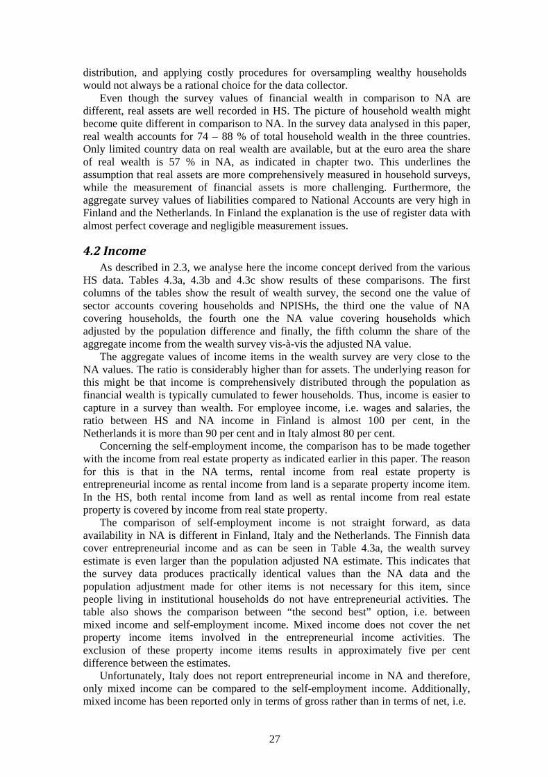
4.2IncomeAs described in 2.3, we analyse here the income concept derived from the various

HS data. Tables 4.3a, 4.3b and 4.3c show results of these comparisons. The first columns of the tables show the result of wealth survey, the second one the value of sector accounts covering households and NPISHs, the third one the value of NA covering households, the fourth one the NA value covering households which adjusted by the population difference and finally, the fifth column the share of the aggregate income from the wealth survey vis-à-vis the adjusted NA value.

The aggregate values of income items in the wealth survey are very close to the NA values. The ratio is considerably higher than for assets. The underlying reason for this might be that income is comprehensively distributed through the population as financial wealth is typically cumulated to fewer households. Thus, income is easier to capture in a survey than wealth. For employee income, i.e. wages and salaries, the ratio between HS and NA income in Finland is almost 100 per cent, in the Netherlands it is more than 90 per cent and in Italy almost 80 per cent.

Concerning the self-employment income, the comparison has to be made together with the income from real estate property as indicated earlier in this paper. The reason for this is that in the NA terms, rental income from real estate property is entrepreneurial income as rental income from land is a separate property income item. In the HS, both rental income from land as well as rental income from real estate property is covered by income from real state property.

The comparison of self-employment income is not straight forward, as data availability in NA is different in Finland, Italy and the Netherlands. The Finnish data cover entrepreneurial income and as can be seen in Table 4.3a, the wealth survey estimate is even larger than the population adjusted NA estimate. This indicates that the survey data produces practically identical values than the NA data and the population adjustment made for other items is not necessary for this item, since people living in institutional households do not have entrepreneurial activities. The table also shows the comparison between “the second best” option, i.e. between mixed income and self-employment income. Mixed income does not cover the net property income items involved in the entrepreneurial income activities. The exclusion of these property income items results in approximately five per cent difference between the estimates.

Unfortunately, Italy does not report entrepreneurial income in NA and therefore, only mixed income can be compared to the self-employment income. Additionally, mixed income has been reported only in terms of gross rather than in terms of net, i.e.

28 

the concept covers the consumption of fixed capital. Therefore, the net mixed income had to be estimated by breaking the consumption fixed capital to the part which is related to the mixed income and to the part which is related to the operational surplus. This is estimated by breaking the consumption of fixed capital by the share of gross mixed income of the aggregate of the gross mixed income and operation surplus. As can be seen in table 4.3b, the HS aggregate is high, i.e. almost 90 per cent of the NA aggregate.

From the entrepreneurial income point of view, the data situation is worst in the Netherlands as they have only mixed income and operational surplus aggregate available. The operational surplus is the income flow which is estimated for the imputed rents. As can be seen in Table 4.3c, the self-employment income of the HS data corresponds approximately 50 per cent of this aggregate.

 Table 4.3a Aggregate value of household survey income items compared to

the NA (values Mio €) – Finland. The numbers in italic refer to an estimated value.

  

  

HS

  

NA NA Households

 NA Adjusted

HS, % of NA

Employee income 71,520 73,252 73,252 71,860 99.5% Self-employment income+income from real estate property

         

...vis-à-vis net entrepreunerial income+received rents from land

  

6,879  

6,985  

6,905

  

6,774  

101.6% ...vis-à-vis net mixed income+received rents from land

  

6,879  

7,407  

7,387

  

7,247  

94.9% Social benefits 32,234 32,839 32,839 32,215 100.1% Income from financial investments

 3,541 5,389 4,877

 4,784 74.0%

Income from private business excl. self-employment

 . 1,288 1,288

 1,264

 

Other income 99        Entrepreneurial income + property income

 10,420 14,084 13,552

 13,295 78.4%

Source: Authors’ calculations and Statistics Finland.

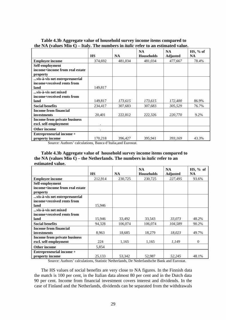
29 

  

Table 4.3b Aggregate value of household survey income items compared to the NA (values Mio €) – Italy. The numbers in italic refer to an estimated value.

   HS NA

NA Households

NA Adjusted

HS, % of NA

Employee income 374,692 481,034 481,034 477,667 78.4% Self-employment income+income from real estate property

         

...vis-à-vis net entrepreunerial income+received rents from land

  

149,817

       

...vis-à-vis net mixed income+received rents from land

  

149,817  

173,615  

173,615

  

172,400  

86.9% Social benefits 234,417 307,683 307,683 305,529 76.7% Income from financial investments

 20,401 222,812 222,326

 220,770 9.2%

Income from private business excl. self-employment

 .

       

Other income .        Entrepreneurial income + property income

 170,218 396,427 395,941

 393,169 43.3%

Source: Authors’ calculations, Banca d’Italia,and Eurostat.  

Table 4.3b Aggregate value of household survey income items compared to the NA (values Mio €) – the Netherlands. The numbers in italic refer to an estimated value.

   HS NA

NA Households

NA Adjusted

HS, % of NA

Employee income 212,914 230,725 230,725 227,495 93.6% Self-employment income+income from real estate property

         

...vis-à-vis net entrepreunerial income+received rents from land

  

15,946

       

...vis-à-vis net mixed income+received rents from land

  

15,946  

33,492  

33,543

  

33,073  

48.2% Social benefits 94,328 106,074 106,074 104,589 90.2% Income from financial investments

 8,963 18,685 18,279

 18,023 49.7%

Income from private business excl. self-employment

 224 1,165 1,165

 1,149 0

Other income 5,854        Entrepreneurial income + property income

 25,133 53,342 52,987

 52,245 48.1%

Source: Authors’ calculations, Statistic Netherlands, De Nederlandsche Bank and Eurostat.  

The HS values of social benefits are very close to NA figures. In the Finnish data the match is 100 per cent, in the Italian data almost 80 per cent and in the Dutch data 90 per cent. Income from financial investment covers interest and dividends. In the case of Finland and the Netherlands, dividends can be separated from the withdrawals

30 

from the quasi-corporations but for Italy there were not this breakdown available and therefore, the aggregate “distributed income of corporations” has been used in the Italian comparison. The comparability of this item is already considerable worse than other items. In Finland the HS value is roughly 75 per cent, in the Netherlands 50 per cent and in Italy less than 10 per cent of the NA value. In the Italian case the large difference is explained by the fact that the withdrawals from quasi-corporations are included in the NA figure.

 The large part of differences is explained by conceptual issues. In the case of the

NA, the property income includes also property income related self-employment income. From this point of view, an appropriate way of comparing these items would be to compare entrepreneurial income and property income together as it is done on the last line of the comparison. Withdrawals from quasi-corporations, which are assumed to be comparable with the HS item “income from private business excluding self-employment”, are causing the problem as only in the case of the Netherlands these are reported as a part of the wealth survey. The difference between these items seems to be large. Additionally, as mentioned earlier in the case of Italy, it is not possible to separate withdrawals from the other distributed income of corporations. For property income and entrepreneurial income, the HS aggregate is in Finland almost 80 per cent, in Italy almost 45 per cent and in the Netherlands almost 50 per cent of the NA aggregate.

 

4.3BreakdownofwealthThe final step in the joint analysis of these data sources is breaking down macro

data to groups of households with the help of micro data. In this paper, the emphasis is on modified financial wealth, definitions being comparable between the two sources. Two household classifications are used based on the work by OECD Expert Group on Disparities in a National Accounts Framework: household type and main source of income. In addition to the breakdowns the significance of adjusting modified financial wealth on the distribution of total financial wealth and total wealth is analysed.

Breaking down NA data on modified financial wealth for household groups is done in two steps. First, values for each of the four individual financial assets are broken down by household groups using data from the micro source. Secondly, the aggregate values from NA (adjusted for NPISH’s and population coverage) are multiplied with the shares obtained in step one for each asset and each group of households.

The methodology used relies on the assumption that that the rate of under- reporting, whether related to households under-reporting the value of an existing item or to households not reporting having an existing item, is assumed to be randomly distributed across groups of households. The same approach is used in the Eurostat/OECD Expert group on Disparities in a National Accounts framework for breaking down income and consumption items that exist in both micro and macro sources. Although analyses done on the Swedish data show that there might be a correlation between asset values and reporting errors21, the results might not be applicable to other countries or surveys, and there is not sufficient information on feasible correction factors that could be used for different household subgroups. Due

  

21 See Klevmarken and Johansson (2007). They conclude that there is a negative correlation between reporting errors and values of the main residence and some financial assets in the Swedish case.

31 

to conceptual discrepancies, breaking down other asset types from NA does not seem a feasible option. However, the distributional impact of adjusting modified financial wealth to the NA level can be presented. The adjusted wealth concept used in the remaining part of this paper will thus consist of:

1) Modified financial assets (deposits, bonds, mutual funds and quoted shares): levels taken from NA, distribution from HS data

2) Other financial assets (pensions, unquoted shares, other financial assets): levels and distribution taken from HS data, recognising the lack of coverage to NA

3) Real assets: level and distribution taken from HS data, no information on coverage available, but coverage can be assumed to be relatively good.

Hence, this exercise could be interpreted rather as an adjustment of survey data than as a breakdown of NA.

Shares of asset values included in modified financial wealth by household groups in HS data are shown in Annex tables A1a-c, together with the population shares of corresponding groups. Annex tables A2a-c show the results of the breakdown of modified financial wealth by items.

Table 4.4 indicates the distribution of aggregate wealth items in HS data, both before and after NA adjustment. In Finland the significance of modified financial wealth is bigger in the original survey data, especially in relation to total financial wealth. One main reason for this is that the register-based data does not capture self- employment businesses very comprehensively in comparison to survey data. Naturally, the lower the coverage of assets included in modified financial is, the bigger the impact of adjustment to NA. As a result of adjustment to national account, the share of modified financial wealth in total wealth is 20 – 24 % and the share of financial wealth 22 – 37 % of total wealth.

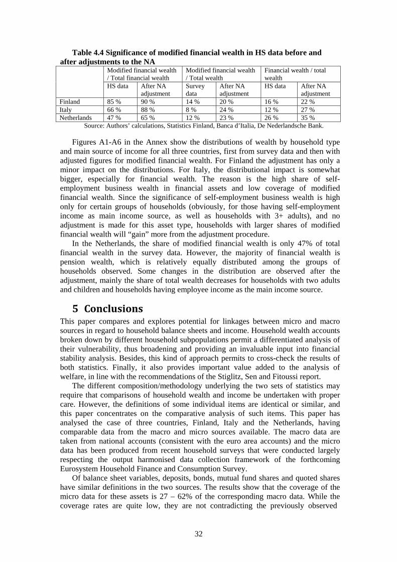
32 

Table 4.4 Significance of modified financial wealth in HS data before and after adjustments to the NA

  Modified financial wealth / Total financial wealth

Modified financial wealth / Total wealth

Financial wealth / total wealth

HS data After NA adjustment

Survey data

After NA adjustment

HS data After NA adjustment

Finland 85 % 90 % 14 % 20 % 16 % 22 % Italy 66 % 88 % 8 % 24 % 12 % 27 % Netherlands 47 % 65 % 12 % 23 % 26 % 35 %

Source: Authors’ calculations, Statistics Finland, Banca d’Italia, De Nederlandsche Bank.  

Figures A1-A6 in the Annex show the distributions of wealth by household type and main source of income for all three countries, first from survey data and then with adjusted figures for modified financial wealth. For Finland the adjustment has only a minor impact on the distributions. For Italy, the distributional impact is somewhat bigger, especially for financial wealth. The reason is the high share of self- employment business wealth in financial assets and low coverage of modified financial wealth. Since the significance of self-employment business wealth is high only for certain groups of households (obviously, for those having self-employment income as main income source, as well as households with 3+ adults), and no adjustment is made for this asset type, households with larger shares of modified financial wealth will “gain” more from the adjustment procedure.

In the Netherlands, the share of modified financial wealth is only 47% of total financial wealth in the survey data. However, the majority of financial wealth is pension wealth, which is relatively equally distributed among the groups of households observed. Some changes in the distribution are observed after the adjustment, mainly the share of total wealth decreases for households with two adults and children and households having employee income as the main income source.

 

5ConclusionsThis paper compares and explores potential for linkages between micro and macro sources in regard to household balance sheets and income. Household wealth accounts broken down by different household subpopulations permit a differentiated analysis of their vulnerability, thus broadening and providing an invaluable input into financial stability analysis. Besides, this kind of approach permits to cross-check the results of both statistics. Finally, it also provides important value added to the analysis of welfare, in line with the recommendations of the Stiglitz, Sen and Fitoussi report.

The different composition/methodology underlying the two sets of statistics may require that comparisons of household wealth and income be undertaken with proper care. However, the definitions of some individual items are identical or similar, and this paper concentrates on the comparative analysis of such items. This paper has analysed the case of three countries, Finland, Italy and the Netherlands, having comparable data from the macro and micro sources available. The macro data are taken from national accounts (consistent with the euro area accounts) and the micro data has been produced from recent household surveys that were conducted largely respecting the output harmonised data collection framework of the forthcoming Eurosystem Household Finance and Consumption Survey.

Of balance sheet variables, deposits, bonds, mutual fund shares and quoted shares have similar definitions in the two sources. The results show that the coverage of the micro data for these assets is 27 – 62% of the corresponding macro data. While the coverage rates are quite low, they are not contradicting the previously observed

33 

difficulties in collecting data on financial assets from household surveys. The coverage of the income items is systematically higher than in the case of the wealth items. The underlying reason for different coverage of income and wealth might be that income is comprehensively and more equally distributed through the population compared to financial wealth and therefore, aggregate levels of income are easier to capture in surveys.

Data collection methods seem to explain the differences in the coverage of financial wealth only partially, primarily in Finland where the values for balance sheet items were collected from registers and through register-based estimations of varying quality. Probably the main lesson to be learned from this analysis is that to achieve better coverage the importance of collecting data from the wealthiest households (i.e. oversampling the wealthy) should be stressed. This is of special importance for items that are owned only by a small share of households.

It should be emphasised that the low coverage of financial wealth in comparison to national accounts restricts the analytical power of survey data only to some extent. Household surveys on wealth are, after all, conducted to make several kinds of analyses on all parts of the wealth distribution, not only on the wealthy. While low coverage rates suggest that data on the wealthiest households are somewhat biased, the negative impact on data quality for other parts of the distribution might be limited, given that most households do not own any other financial assets than deposits. Naturally, the general picture of wealth inequality will suffer from the inability to collect data from, the top fractions of the distribution in household surveys.

Coverage issues might also be explained by the production process of national accounts figures. To satisfy balancing constraints, national accounts do not primarily aim to minimize bias in the household sector, but to minimize bias in the estimates for the economy as a whole. For example, if certain economic transactions for the household sector are derived as a residual, i.e. by subtracting from the estimated total the estimates of other institutional sectors, the level of household wealth and income will be overestimated in the macro source.

Survey data enables breaking down national accounts by groups of households, and this is among the first attempts to do this for wealth items. Due to conceptual issues and no data availability on real assets in national accounts, only the levels of deposits, bonds, mutual funds and quoted shares are adjusted to national accounts levels. The impact of this adjustment on the wealth distribution observed in the survey data was negligible in Finland, and only somewhat noticeable for certain individual household groups in Italy and the Netherlands.

Finally, it can be concluded that this is a useful first step in building linkage between wealth surveys and national accounts. However, there is still much to improve. For instance, there is room for development in the area of measuring household real assets in national accounts and improving the conceptual analysis of pensions and business wealth between the two sources. Additionally, as the results of the HFCS become available at the beginning of 2013, the framework applied to the analysis of country data can be extended to the euro area aggregate, in both cases based on consistent output-harmonised micro datasets.

34 

 

 

6References 

 Antoniewicz, R., Bonci R., Generale A., Marchese G., Neri A., Maser K. and O’Hagan P. (2005): “Household Wealth: Comparing Micro and Macro Data in Cyprus, Canada, Italy and United States”, paperi, joka on esitetty: LWS Workshop: “Construction and Usage of Comparable Microdata on Wealth: the LWS”, Banca d’Italia, Perugia, Italy, 27-29 January 2005.

 Castrén, Olli and Kavonius, Ilja Kristian (2009): Balance Sheet Interlinkages and Macro-Financial Risk Analysis in the Euro Area, Working Papers 1124, European Central Bank, Frankfurt am Main 2009.  Durier, Sébastien and Lucile Richet-Mastain (2012): Distributional Information on Income and Wealth Using French Households Micro Data and National Accounts. Paper Prepared for the 32nd General Conference of The International Association for Research in Income and Wealth, Boston, August 5 – 12. 2012.  

European System of Accounts 1995 (ESA95), Council (EC) Regulation No 2223/96 of 25 June 1996 on the European system of national and regional accounts in the Community, Official Journal of the European Union L 310/1-469.

 Fessler, Pirmin, Maximilian Kasy and Peter Lindner (2012): Survey Mode Effects on Income Inequality Measurement. Paper Prepared for the 32nd General Conference of The International Association for Research in Income and Wealth, Boston, August 5 – 12. 2012.  HFCN (2008): Household Finance and Consumption Survey: Modalities for Implementation. Household Finance and Consumption Network, European Central Bank.  HFCNECB (2008): Estimating entitlements in retirement plans. Household Finance and Consumption Network, European Central Bank.  HFCNECB (2010). List of Core Output Variables, Household Finance and Consumption Survey. ECB & Household Finance and Consumption Network.

 

  

Johansson, Fredrik and Andres Klevmarken (2007): Comparing Register and Survey Wealth Data. In: “Essays on Measurement Error and Nonresponse”. Uppsala University Economic Studies 103, pp. 47 – 76.

 Juster, F. Thomas, James P. Smith and Frank Stafford (1999): The Measurement and Structure of Household Wealth. Labour Economics, Vol. 6,pp. 253 – 275.

 Kavonius, Ilja Kristian (2006): “The Implication of Employee Stock Options and Holding Gains for Disposable Income and Household Saving Rates in Finland”, Journal of Official Statistics, 3/ Volume 22, 2006, pp. 585–597, Statistics Sweden.

 Kavonius, Ilja Kristian & Törmälehto, V-M (2010): “Integrating Micro and Macro Accounts – The Linkages Between Euro Area Household Wealth Survey and Aggregate Balance Sheets

35 

for Households”, IARIW 31st General Conference, St-Gallen, Switzerland, August 22-28, 2010

 Kennickell, A. (2007), “The Role of Over-sampling of the Wealthy in the Survey of Consumer Finances”, Federal Reserve Board, Survey of Consumer Finances Working Papers, July 2007.

 Martin, Peter and Peter Lynn (2011): The Effects of Mixed Mode Survey Designson Simple and Complex Analyses. Centre for Comparative Social Surveys Working Paper Series, No 4.

 Pérez-Duarte S., Sánchez-Muñoz C., Törmälehto V-M: “Re-weighting to reduce unit non- response bias in household wealth surveys: a cross-country comparative perspective illustrated by a case study.” Paper prepared for the Conference on European Quality in Statistics, Helsinki, May 4-6 2010.

 Revilla, Melanie (2010): Quality in Unimode and Mixed-Mode Designs: A Multitrait- Multimethod Approach. Survey Research Methods, Vol 4, No 3, pp. 151-164.

 Rubin, Donald R. (1987): Multiple Imputation for Nonresponse in Surveys. John Wiley & Sons.

 System of National Accounts 1993 (SNA93), Commission of the European Communities, International Monetary Fund, United Nations, World Bank, Brussels/Luxembourg, New York, Paris, Washington D.C., 1993.

 System of National Accounts 2008 (SNA2008), Commission of the European Communities, International Monetary Fund, United Nations, World Bank, Brussels/Luxembourg, unpublished.

 Stiglitz, J.E & Sen, A. & Fitoussi, J-P (2009): Report by the Commission on the Measurement of EconomicPerformance and Social Progress, www.stiglitz-sen-fitoussi.fr.

 

Van den Heede, Aaron, Tim Goedemé, Karel van den Bosch and Josefine Vanhille (2012): What Difference Does a Survey Make? Comparing Incomes of the 65+ in Europe Between SILC and SHARE. Paper Prepared for the 32nd General Conference of The International Association for Research in Income and Wealth, Boston, August 5 – 12. 2012.

 Verma, Vijay & Betti, Gianni (2010): “Data Accuracy in EU-SILC”. In Atkinson, Anthony B. and Marlier, Eric (ed.): Income and Living Conditions in Europe. Eurostat 2010.

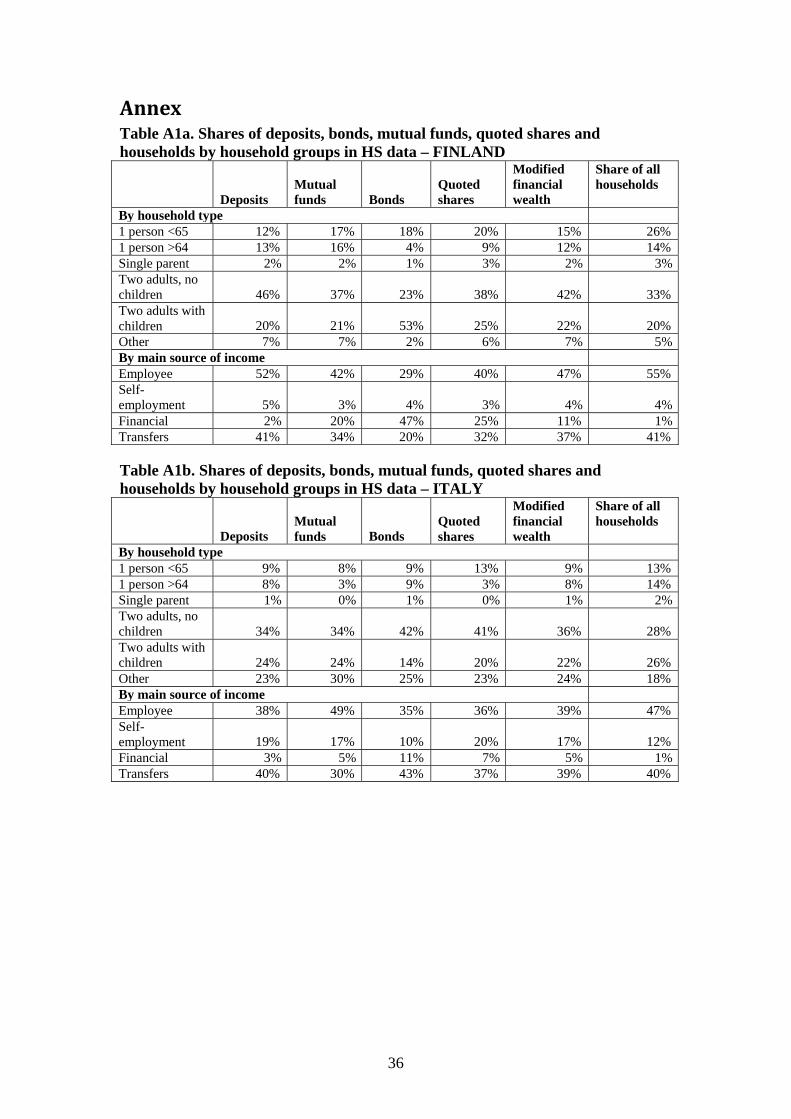
36 

AnnexTable A1a. Shares of deposits, bonds, mutual funds, quoted shares and households by household groups in HS data – FINLAND

    

Deposits

 Mutual funds

 Bonds

Quoted shares

Modified financial wealth

Share of all households

By household type  1 person <65 12% 17% 18% 20% 15% 26% 1 person >64 13% 16% 4% 9% 12% 14% Single parent 2% 2% 1% 3% 2% 3%Two adults, no children

 46%

 37% 23% 38% 42%

 33%

Two adults with children

 20%

 21% 53% 25% 22%

 20%

Other 7% 7% 2% 6% 7% 5%By main source of income  Employee 52% 42% 29% 40% 47% 55% Self- employment

 5%

 3% 4% 3% 4%

 4%

Financial 2% 20% 47% 25% 11% 1%Transfers 41% 34% 20% 32% 37% 41%

 

Table A1b. Shares of deposits, bonds, mutual funds, quoted shares and households by household groups in HS data – ITALY

   

 Deposits

 Mutual funds

 Bonds

Quoted shares

Modified financial wealth

Share of all households

By household type  1 person <65 9% 8% 9% 13% 9% 13% 1 person >64 8% 3% 9% 3% 8% 14% Single parent 1% 0% 1% 0% 1% 2%Two adults, no children

 34%

 34% 42% 41% 36%

 28%

Two adults with children

 24%

 24% 14% 20% 22%

 26%

Other 23% 30% 25% 23% 24% 18% By main source of income  Employee 38% 49% 35% 36% 39% 47% Self- employment

 19%

 17% 10% 20% 17%

 12%

Financial 3% 5% 11% 7% 5% 1%Transfers 40% 30% 43% 37% 39% 40%

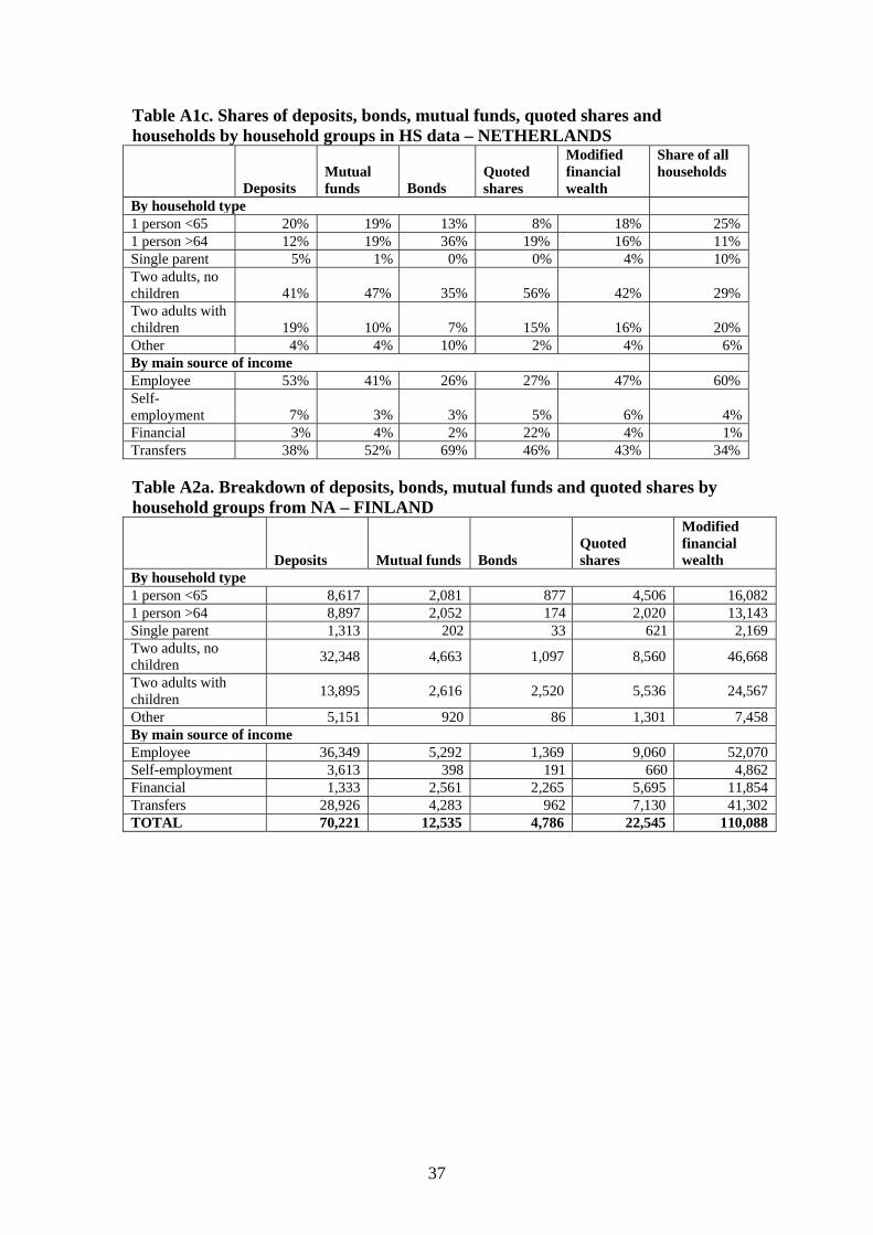
37 

Table A1c. Shares of deposits, bonds, mutual funds, quoted shares and households by household groups in HS data – NETHERLANDS

   

 Deposits

 Mutual funds

 Bonds

Quoted shares

Modified financial wealth

Share of all households

By household type  1 person <65 20% 19% 13% 8% 18% 25% 1 person >64 12% 19% 36% 19% 16% 11% Single parent 5% 1% 0% 0% 4% 10% Two adults, no children

 41%

 47% 35% 56% 42%

 29%

Two adults with children

 19%

 10% 7% 15% 16%

 20%

Other 4% 4% 10% 2% 4% 6%By main source of income  Employee 53% 41% 26% 27% 47% 60% Self- employment

 7%

 3% 3% 5% 6%

 4%

Financial 3% 4% 2% 22% 4% 1%Transfers 38% 52% 69% 46% 43% 34%

 

Table A2a. Breakdown of deposits, bonds, mutual funds and quoted shares by household groups from NA – FINLAND

  

Deposits  

Mutual funds  

Bonds Quoted shares

Modified financial wealth

By household type 1 person <65 8,617 2,081 877 4,506 16,082 1 person >64 8,897 2,052 174 2,020 13,143 Single parent 1,313 202 33 621 2,169 Two adults, no children

32,348 4,663 1,097 8,560  

46,668

Two adults with children

13,895 2,616 2,520 5,536  

24,567

Other 5,151 920 86 1,301 7,458 By main source of income Employee 36,349 5,292 1,369 9,060 52,070 Self-employment 3,613 398 191 660 4,862 Financial 1,333 2,561 2,265 5,695 11,854 Transfers 28,926 4,283 962 7,130 41,302 TOTAL 70,221 12,535 4,786 22,545 110,088

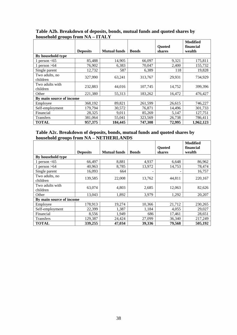
38 

Table A2b. Breakdown of deposits, bonds, mutual funds and quoted shares by household groups from NA – ITALY

   

 Deposits

 Mutual funds

 Bonds

Quoted shares

Modified financial wealth

By household type 1 person <65 85,488 14,905 66,097 9,321 175,811 1 person >64 76,902 6,383 70,047 2,400 155,732 Single parent 12,732 587 6,389 118 19,828 Two adults, no children

 

327,990 63,241 313,767 29,931  

734,929

Two adults with children

 

232,883 44,016 107,745 14,752  

399,396

Other 221,380 55,313 183,262 16,472 476,427 By main source of income Employee 368,192 89,821 261,599 26,615 746,227 Self-employment 179,794 30,572 76,871 14,496 301,733 Financial 28,325 9,011 85,269 5,147 127,751 Transfers 381,064 55,041 323,569 26,738 786,411 TOTAL 957,375 184,445 747,308 72,995 1,962,123

 

Table A2c. Breakdown of deposits, bonds, mutual funds and quoted shares by household groups from NA – NETHERLANDS

    

Deposits  

Mutual funds  

Bonds Quoted shares

Modified financial wealth

By household type 1 person <65 66,497 8,881 4,937 6,648 86,962 1 person >64 40,963 8,785 13,972 14,753 78,474 Single parent 16,093 664 - - 16,757 Two adults, no children

 

139,585 22,008 13,762 44,811  

220,167

Two adults with children

 

63,074 4,803 2,685 12,063  

82,626

Other 13,043 1,892 3,979 1,292 20,207 By main source of income Employee 178,913 19,274 10,366 21,712 230,265 Self-employment 22,399 1,387 1,184 4,055 29,027 Financial 8,556 1,949 686 17,461 28,651 Transfers 129,387 24,424 27,099 36,340 217,249 TOTAL 339,255 47,034 39,336 79,568 505,192

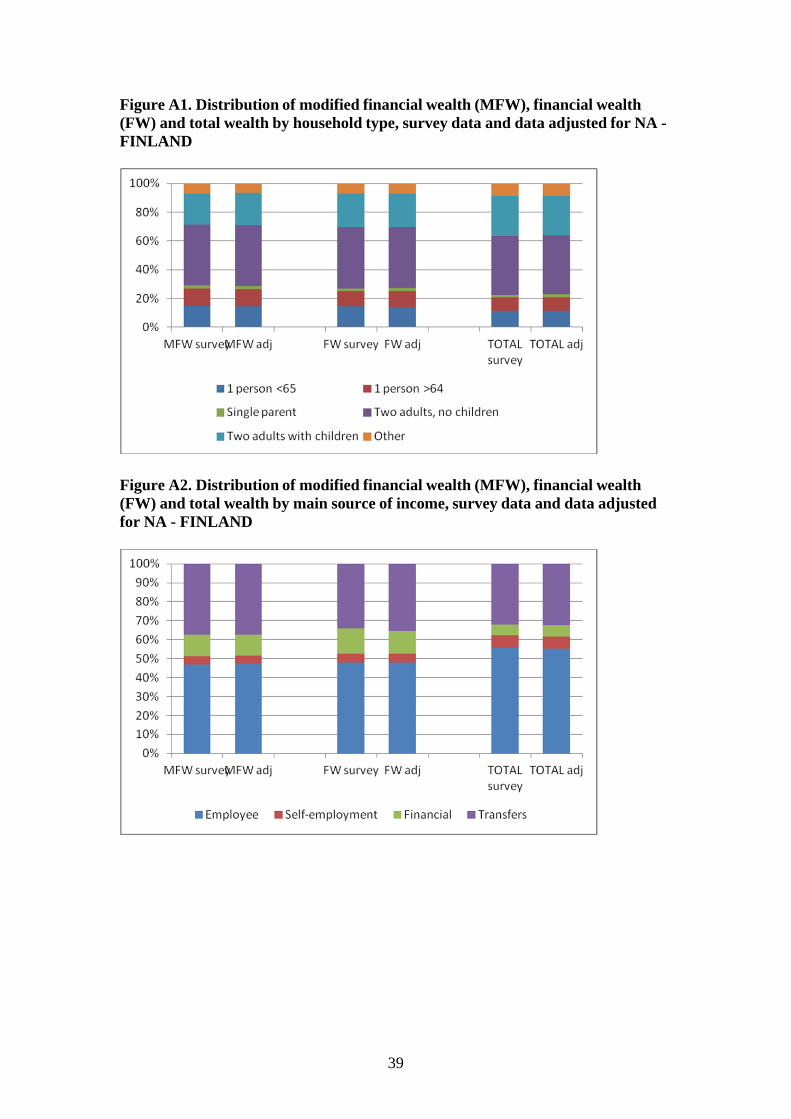
39 

Figure A1. Distribution of modified financial wealth (MFW), financial wealth (FW) and total wealth by household type, survey data and data adjusted for NA - FINLAND  

 

 

Figure A2. Distribution of modified financial wealth (MFW), financial wealth (FW) and total wealth by main source of income, survey data and data adjusted for NA - FINLAND  

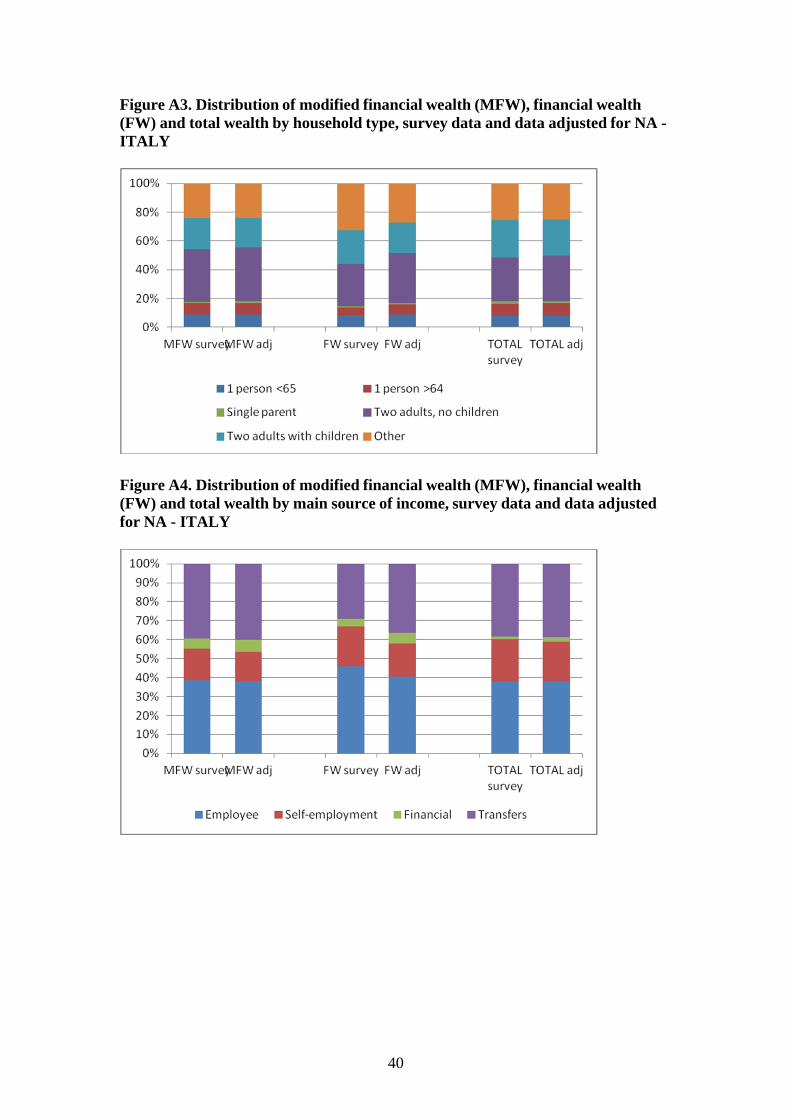
40 

Figure A3. Distribution of modified financial wealth (MFW), financial wealth (FW) and total wealth by household type, survey data and data adjusted for NA - ITALY  

 

 

Figure A4. Distribution of modified financial wealth (MFW), financial wealth (FW) and total wealth by main source of income, survey data and data adjusted for NA - ITALY  

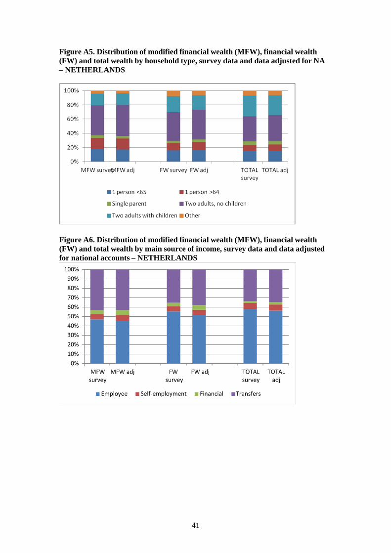
41 

Figure A5. Distribution of modified financial wealth (MFW), financial wealth (FW) and total wealth by household type, survey data and data adjusted for NA – NETHERLANDS  

 

 

Figure A6. Distribution of modified financial wealth (MFW), financial wealth (FW) and total wealth by main source of income, survey data and data adjusted for national accounts – NETHERLANDS

100% 

90% 

80% 

70% 

60% 

50% 

40% 

30% 

20% 

10% 

0% 

MFW survey 

MFW adj  FW survey 

FW adj  TOTAL survey 

TOTAL adj 

 

Employee  Self‐employment  Financial  Transfers