Embed Size (px)
Citation preview

Eulerian Polynomials and Beyond
Michelle WachsUniversity of Miami
Based on joint work with John Shareshian
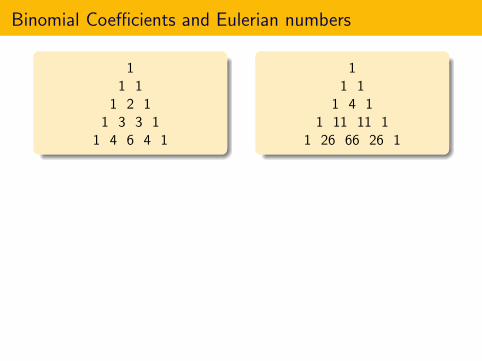
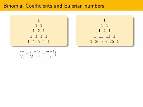
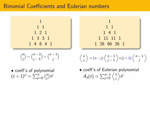
Binomial Coefficients and Eulerian numbers
11 1
1 2 11 3 3 1
1 4 6 4 1
11 1
1 4 11 11 11 1
1 26 66 26 1
(nj
)=(n − 1
j − 1
)+(n − 1
j
) ⟨nj
⟩= (n − j)
⟨n − 1j − 1
⟩+(j + 1)
⟨n − 1
j
⟩
• coeff’s of polynomial(t + 1)n =
∑nj=0
(nj
)t j
• coeff’s of Eulerian polynomial
An(t) =∑n−1
j=0
⟨nj
⟩t j
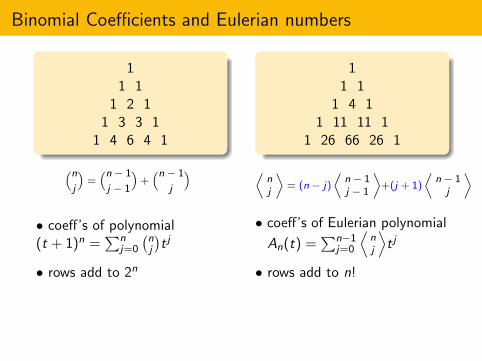
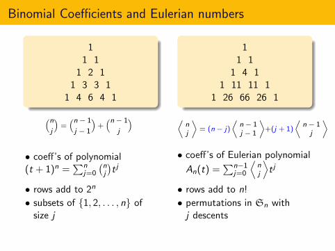
• rows add to 2n • rows add to n!
• subsets of {1, 2, . . . , n} ofsize j
• permutations in Sn withj descents
• Rows are palindromic and unimodal.
Binomial Coefficients and Eulerian numbers
11 1
1 2 11 3 3 1
1 4 6 4 1
11 1
1 4 11 11 11 1
1 26 66 26 1
(nj
)=(n − 1
j − 1
)+(n − 1
j
)
⟨nj
⟩= (n − j)
⟨n − 1j − 1
⟩+(j + 1)
⟨n − 1
j
⟩
• coeff’s of polynomial(t + 1)n =
∑nj=0
(nj
)t j
• coeff’s of Eulerian polynomial
An(t) =∑n−1
j=0
⟨nj
⟩t j
• rows add to 2n • rows add to n!
• subsets of {1, 2, . . . , n} ofsize j
• permutations in Sn withj descents
• Rows are palindromic and unimodal.
Binomial Coefficients and Eulerian numbers
11 1
1 2 11 3 3 1
1 4 6 4 1
11 1
1 4 11 11 11 1
1 26 66 26 1
(nj
)=(n − 1
j − 1
)+(n − 1
j
) ⟨nj
⟩= (n − j)
⟨n − 1j − 1
⟩+(j + 1)
⟨n − 1
j
⟩
• coeff’s of polynomial(t + 1)n =
∑nj=0
(nj
)t j
• coeff’s of Eulerian polynomial
An(t) =∑n−1
j=0
⟨nj
⟩t j
• rows add to 2n • rows add to n!
• subsets of {1, 2, . . . , n} ofsize j
• permutations in Sn withj descents
• Rows are palindromic and unimodal.
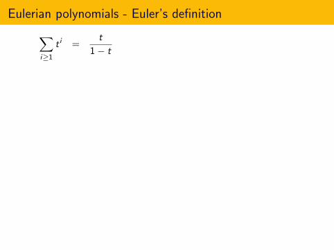
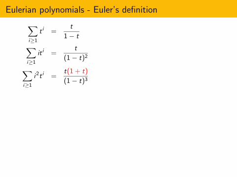
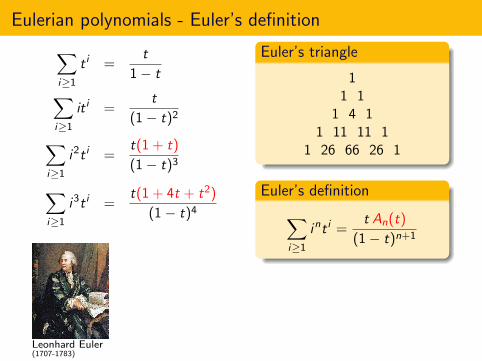
Eulerian polynomials - Euler’s definition
∑i≥1
t i =t
1− t
∑i≥1
it i =t
(1− t)2
∑i≥1
i2t i =t(1 + t)
(1− t)3
∑i≥1
i3t i =t(1 + 4t + t2)
(1− t)4
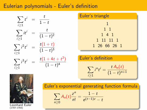
Euler’s triangle
11 1
1 4 11 11 11 1
1 26 66 26 1
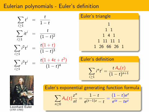
Euler’s definition∑i≥1
int i =t An(t)
(1− t)n+1
Leonhard Euler(1707-1783)
Euler’s exponential generating function formula∑n≥0
An(t)zn
n!=
1− t
e(t−1)z − t=
(1− t)ez
etz − tez

Eulerian polynomials - Euler’s definition
∑i≥1
t i =t
1− t∑i≥1
it i =t
(1− t)2
∑i≥1
i2t i =t(1 + t)
(1− t)3
∑i≥1
i3t i =t(1 + 4t + t2)
(1− t)4
Euler’s triangle
11 1
1 4 11 11 11 1
1 26 66 26 1
Euler’s definition∑i≥1
int i =t An(t)
(1− t)n+1
Leonhard Euler(1707-1783)
Euler’s exponential generating function formula∑n≥0
An(t)zn
n!=
1− t
e(t−1)z − t=
(1− t)ez
etz − tez
Eulerian polynomials - Euler’s definition
∑i≥1
t i =t
1− t∑i≥1
it i =t
(1− t)2
∑i≥1
i2t i =t(1 + t)
(1− t)3
∑i≥1
i3t i =t(1 + 4t + t2)
(1− t)4
Euler’s triangle
11 1
1 4 11 11 11 1
1 26 66 26 1
Euler’s definition∑i≥1
int i =t An(t)
(1− t)n+1
Leonhard Euler(1707-1783)
Euler’s exponential generating function formula∑n≥0
An(t)zn
n!=
1− t
e(t−1)z − t
=(1− t)ez
etz − tez
Eulerian polynomials - Euler’s definition
∑i≥1
t i =t
1− t∑i≥1
it i =t
(1− t)2
∑i≥1
i2t i =t(1 + t)
(1− t)3
∑i≥1
i3t i =t(1 + 4t + t2)
(1− t)4
Euler’s triangle
11 1
1 4 11 11 11 1
1 26 66 26 1
Euler’s definition∑i≥1
int i =t An(t)
(1− t)n+1
Leonhard Euler(1707-1783)
Euler’s exponential generating function formula∑n≥0
An(t)zn
n!=
1− t
e(t−1)z − t=
(1− t)ez
etz − tez
Eulerian numbers - combinatorial interpretation
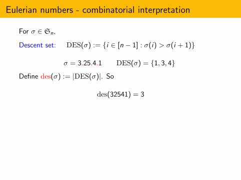
For σ ∈ Sn,
Descent set: DES(σ) := {i ∈ [n − 1] : σ(i) > σ(i + 1)}
σ = 3.25.4.1 DES(σ) = {1, 3, 4}
Define des(σ) := |DES(σ)|. So
des(32541) = 3
Excedance set: EXC(σ) := {i ∈ [n − 1] : σ(i) > i}
σ = 32541 EXC(σ) = {1, 3}
Define exc(σ) := |EXC(σ)|. So
exc(32541) = 2

Eulerian numbers - combinatorial interpretation
For σ ∈ Sn,
Descent set: DES(σ) := {i ∈ [n − 1] : σ(i) > σ(i + 1)}
σ = 3.25.4.1 DES(σ) = {1, 3, 4}
Define des(σ) := |DES(σ)|. So
des(32541) = 3
Excedance set: EXC(σ) := {i ∈ [n − 1] : σ(i) > i}
σ = 32541 EXC(σ) = {1, 3}
Define exc(σ) := |EXC(σ)|. So
exc(32541) = 2
Eulerian numbers - combinatorial interpretation
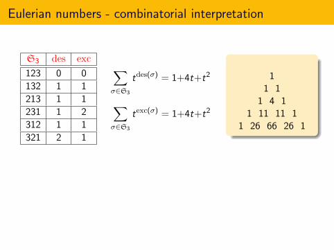
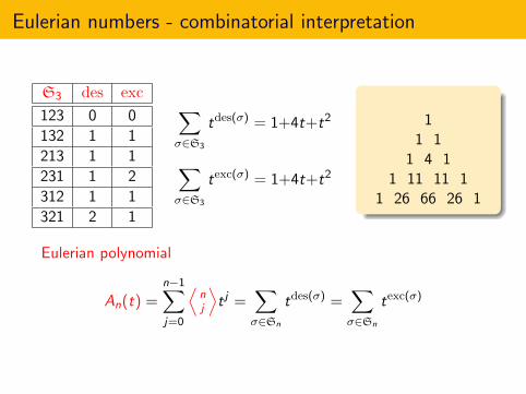
S3 des exc
123 0 0
132 1 1
213 1 1
231 1 2
312 1 1
321 2 1
∑σ∈S3
tdes(σ) = 1+4t+t2
∑σ∈S3
texc(σ) = 1+4t+t2
11 1
1 4 11 11 11 1
1 26 66 26 1
Eulerian polynomial
An(t) =n−1∑j=0
⟨nj
⟩t j =
∑σ∈Sn
tdes(σ) =∑σ∈Sn
texc(σ)
MacMahon (1905) showed equidistribution of des and exc.Carlitz and Riordin (1955) showed equals An(t).
Eulerian numbers - combinatorial interpretation
S3 des exc
123 0 0
132 1 1
213 1 1
231 1 2
312 1 1
321 2 1
∑σ∈S3
tdes(σ) = 1+4t+t2
∑σ∈S3
texc(σ) = 1+4t+t2
11 1
1 4 11 11 11 1
1 26 66 26 1
Eulerian polynomial
An(t) =n−1∑j=0
⟨nj
⟩t j =
∑σ∈Sn
tdes(σ) =∑σ∈Sn
texc(σ)
MacMahon (1905) showed equidistribution of des and exc.Carlitz and Riordin (1955) showed equals An(t).
Unimodality of Eulerian Polynomials
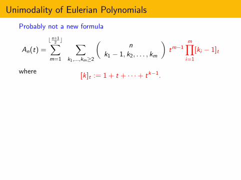
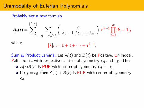
Probably not a new formula
An(t) =
b n+12c∑
m=1
∑k1,...,km≥2
(n
k1 − 1, k2, . . . , km
)tm−1
m∏i=1
[ki − 1]t
where[k]t := 1 + t + · · ·+ tk−1.
Sum & Product Lemma: Let A(t) and B(t) be Positive, Unimodal,Palindromic with respective centers of symmetry cA and cB . Then
A(t)B(t) is PUP with center of symmetry cA + cB .
If cA = cB then A(t) + B(t) is PUP with center of symmetrycA.
Center of symmetry:
(m − 1) +m∑i=1
ki − 2
2=
1
2(n − 1).
Unimodality of Eulerian Polynomials
Probably not a new formula
An(t) =
b n+12c∑
m=1
∑k1,...,km≥2
(n
k1 − 1, k2, . . . , km
)tm−1
m∏i=1
[ki − 1]t
where[k]t := 1 + t + · · ·+ tk−1.
Sum & Product Lemma: Let A(t) and B(t) be Positive, Unimodal,Palindromic with respective centers of symmetry cA and cB . Then
A(t)B(t) is PUP with center of symmetry cA + cB .
If cA = cB then A(t) + B(t) is PUP with center of symmetrycA.
Center of symmetry:
(m − 1) +m∑i=1
ki − 2
2=
1
2(n − 1).
Mahonian Permutation Statistics - q-analogs
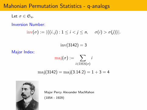
Let σ ∈ Sn.
Inversion Number:
inv(σ) := |{(i , j) : 1 ≤ i < j ≤ n, σ(i) > σ(j)}|.
inv(3142) = 3
Major Index:
maj(σ) :=∑
i∈DES(σ)
i
maj(3142) = maj(3.14.2) = 1 + 3 = 4
Major Percy Alexander MacMahon
(1854 - 1929)

Mahonian Permutation Statistics - q-analogs
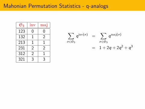
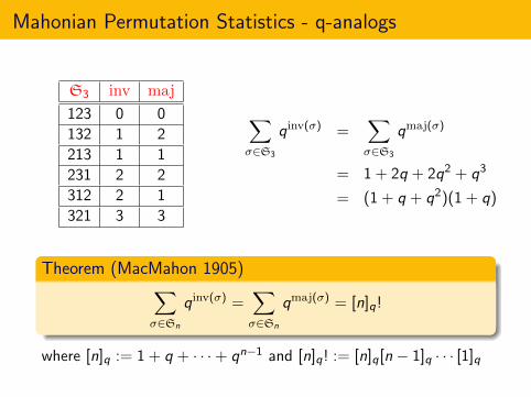
S3 inv maj
123 0 0
132 1 2
213 1 1
231 2 2
312 2 1
321 3 3
∑σ∈S3
qinv(σ) =∑σ∈S3
qmaj(σ)
= 1 + 2q + 2q2 + q3
= (1 + q + q2)(1 + q)
Theorem (MacMahon 1905)∑σ∈Sn
qinv(σ) =∑σ∈Sn
qmaj(σ) = [n]q!
where [n]q := 1 + q + · · ·+ qn−1 and [n]q! := [n]q[n − 1]q · · · [1]q
Mahonian Permutation Statistics - q-analogs
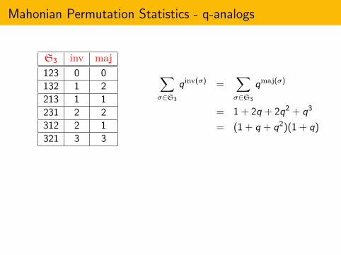
S3 inv maj
123 0 0
132 1 2
213 1 1
231 2 2
312 2 1
321 3 3
∑σ∈S3
qinv(σ) =∑σ∈S3
qmaj(σ)
= 1 + 2q + 2q2 + q3
= (1 + q + q2)(1 + q)
Theorem (MacMahon 1905)∑σ∈Sn
qinv(σ) =∑σ∈Sn
qmaj(σ) = [n]q!
where [n]q := 1 + q + · · ·+ qn−1 and [n]q! := [n]q[n − 1]q · · · [1]q

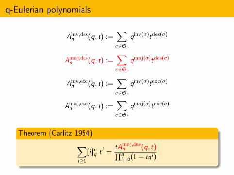
q-Eulerian polynomials
Ainv,desn (q, t) :=
∑σ∈Sn
qinv(σ)tdes(σ)
Amaj,desn (q, t) :=
∑σ∈Sn
qmaj(σ)tdes(σ)
Ainv,excn (q, t) :=
∑σ∈Sn
qinv(σ)texc(σ)
Amaj,excn (q, t) :=
∑σ∈Sn
qmaj(σ)texc(σ)
q-Eulerian polynomials
Ainv,desn (q, t) :=
∑σ∈Sn
qinv(σ)tdes(σ)
Amaj,desn (q, t) :=
∑σ∈Sn
qmaj(σ)tdes(σ)
Ainv,excn (q, t) :=
∑σ∈Sn
qinv(σ)texc(σ)
Amaj,excn (q, t) :=
∑σ∈Sn
qmaj(σ)texc(σ)
Theorem (Carlitz 1954)∑i≥1
[i ]nq t i =tAmaj,des
n (q, t)∏ni=0(1− tqi )
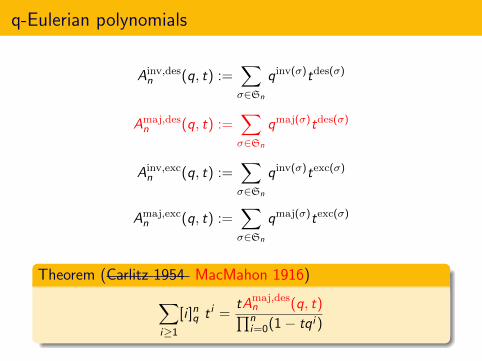
q-Eulerian polynomials
Ainv,desn (q, t) :=
∑σ∈Sn
qinv(σ)tdes(σ)
Amaj,desn (q, t) :=
∑σ∈Sn
qmaj(σ)tdes(σ)
Ainv,excn (q, t) :=
∑σ∈Sn
qinv(σ)texc(σ)
Amaj,excn (q, t) :=
∑σ∈Sn
qmaj(σ)texc(σ)
Theorem (Carlitz 1954 MacMahon 1916)∑i≥1
[i ]nq t i =tAmaj,des
n (q, t)∏ni=0(1− tqi )
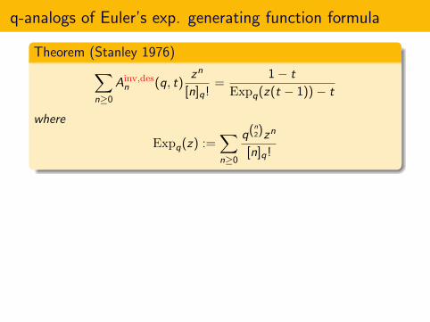
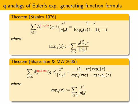
q-analogs of Euler’s exp. generating function formula
Theorem (Stanley 1976)∑n≥0
Ainv,desn (q, t)
zn
[n]q!=
1− t
Expq(z(t − 1))− t
where
Expq(z) :=∑n≥0
q(n2)zn
[n]q!
Theorem (Shareshian & MW 2006)∑n≥0
Amaj,excn (q, t)
zn
[n]q!=
(1− tq) expq(z)
expq(ztq)− tq expq(z)
where
expq(z) :=∑n≥0
zn
[n]q!
q-analogs of Euler’s exp. generating function formula
Theorem (Stanley 1976)∑n≥0
Ainv,desn (q, t)
zn
[n]q!=
1− t
Expq(z(t − 1))− t
where
Expq(z) :=∑n≥0
q(n2)zn
[n]q!
Theorem (Shareshian & MW 2006)∑n≥0
Amaj,excn (q, t)
zn
[n]q!=
(1− tq) expq(z)
expq(ztq)− tq expq(z)
where
expq(z) :=∑n≥0
zn
[n]q!
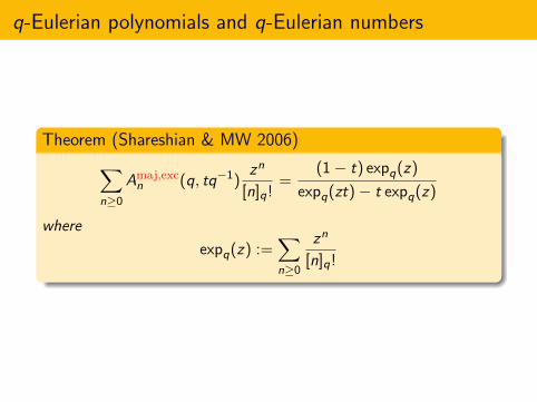
q-Eulerian polynomials and q-Eulerian numbers
Theorem (Shareshian & MW 2006)∑n≥0
Amaj,excn (q, tq−1)
zn
[n]q!=
(1− t) expq(z)
expq(zt)− t expq(z)
where
expq(z) :=∑n≥0
zn
[n]q!

q-Eulerian polynomials and q-Eulerian numbers
Theorem (Shareshian & MW 2006)∑n≥0
Amaj,excn (q, tq−1)
zn
[n]q!=
(1− t) expq(z)
expq(zt)− t expq(z)
where
expq(z) :=∑n≥0
zn
[n]q!
Specialization of (quasi)symmetric function identity∑n≥0
n∑j=0
Qn,j(x)t jzn =(1− t)H(z)
H(zt)− tH(z),
the Qn,j(x) are what we call Eulerian quasisymmetric functions(a sum of certain fundamental quasisymmetric functions)
H(z) :=∑
n≥0 hn(x)zn (complete homogeneous symmetricfunctions)
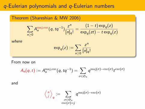
q-Eulerian polynomials and q-Eulerian numbers
Theorem (Shareshian & MW 2006)∑n≥0
Amaj,excn (q, tq−1)
zn
[n]q!=
(1− t) expq(z)
expq(zt)− t expq(z)
where
expq(z) :=∑n≥0
zn
[n]q!
From now on
An(q, t) := Amaj,excn (q, tq−1) =
∑σ∈Sn
qmaj(σ)−exc(σ)texc(σ)
and ⟨nj
⟩q
:=∑σ∈Sn
exc(σ)=j
qmaj(σ)−exc(σ)
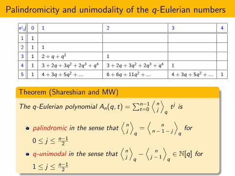
Palindromicity and unimodality of the q-Eulerian numbers
n\j 0 1 2 3 4
1 1
2 1 1
3 1 2 + q + q2 1
4 1 3 + 2q + 3q2 + 2q3 + q4 3 + 2q + 3q2 + 2q3 + q4 1
5 1 4 + 3q + 5q2 + ... 6 + 6q + 11q2 + ... 4 + 3q + 5q2 + ... 1
Theorem (Shareshian and MW)
The q-Eulerian polynomial An(q, t) =∑n−1
t=0
⟨nj
⟩qt j is
palindromic in the sense that⟨
nj
⟩q
=⟨
nn − 1− j
⟩qfor
0 ≤ j ≤ n−12
q-unimodal in the sense that⟨
nj
⟩q−⟨
nj − 1
⟩q∈ N[q] for
1 ≤ j ≤ n−12
Palindromicity and unimodality of the q-Eulerian numbers
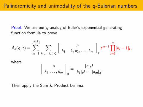
Proof: We use our q-analog of Euler’s exponential generatingfunction formula to prove
An(q, t) =
b n+12c∑
m=1
∑k1,...,km≥2
[n
k1 − 1, k2, . . . , km
]q
tm−1m∏i=1
[ki − 1]t ,
where [n
k1, . . . , km
]q
=[n]q!
[k1]q! · · · [km]q!
Then apply the Sum & Product Lemma.
Geometric Interpretation of the Eulerian numbers
(⟨n0
⟩,⟨
n1
⟩, . . . ,
⟨n
n − 1
⟩)is the h-vector of the type An−1 Coxeter
complex ∆n.
Stanley (1980): The h-vector of every simplicial convex polytope isunimodal (and palindromic).
This is part of the celebrated g -theorem of Billera, Lee and Stanley.
Proof idea: Let P be a d-dimensional convex polytope in Rd withinteger vertices. Let VP be the toric variety associated with P.
Danilov (1978): The h-vector of P equals
(dimH0(VP), dimH2(VP), . . . , dimH2d(VP))
(Hence⟨
nj
⟩= dimH2j(V∆n).)
Geometric Interpretation of the Eulerian numbers
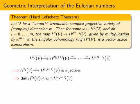
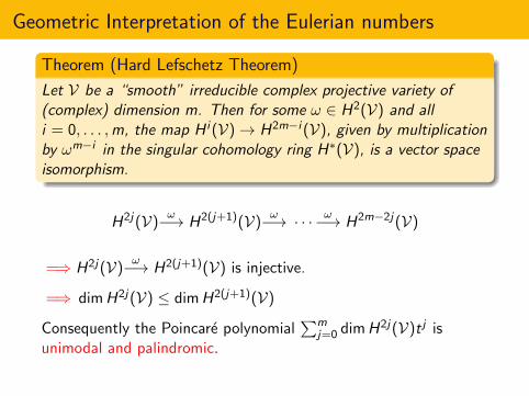
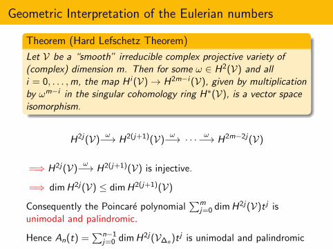
Theorem (Hard Lefschetz Theorem)
Let V be a “smooth” irreducible complex projective variety of(complex) dimension m. Then for some ω ∈ H2(V) and alli = 0, . . . ,m, the map H i (V)→ H2m−i (V), given by multiplicationby ωm−i in the singular cohomology ring H∗(V), is a vector spaceisomorphism.
H2j(V)ω−→ H2(j+1)(V)
ω−→ · · · ω−→ H2m−2j(V)
=⇒ H2j(V)ω−→ H2(j+1)(V) is injective.
=⇒ dimH2j(V) ≤ dimH2(j+1)(V)
Consequently the Poincare polynomial∑m
j=0 dimH2j(V)t j isunimodal and palindromic.
Hence An(t) =∑n−1
j=0 dimH2j(V∆n)t j is unimodal and palindromic
Geometric Interpretation of the Eulerian numbers
Theorem (Hard Lefschetz Theorem)
Let V be a “smooth” irreducible complex projective variety of(complex) dimension m. Then for some ω ∈ H2(V) and alli = 0, . . . ,m, the map H i (V)→ H2m−i (V), given by multiplicationby ωm−i in the singular cohomology ring H∗(V), is a vector spaceisomorphism.
H2j(V)ω−→ H2(j+1)(V)
ω−→ · · · ω−→ H2m−2j(V)
=⇒ H2j(V)ω−→ H2(j+1)(V) is injective.
=⇒ dimH2j(V) ≤ dimH2(j+1)(V)
Consequently the Poincare polynomial∑m
j=0 dimH2j(V)t j isunimodal and palindromic.
Hence An(t) =∑n−1
j=0 dimH2j(V∆n)t j is unimodal and palindromic
Geometric interpretation of the q-Eulerian numbers
There is a natural action of Sn on the toric variety V∆n whichinduces a representation on each H2j(V∆n).
{Representations of Sn}ch−→ Λn
Zpsq−−→ Z[q]
ch: Frobenius characteristicΛnZ: homogeneous symmetric functions over Z of degree n
psq: stable principal specialization.
psq(f (x1, x2, . . . )) = f (1, q, q2, . . . )n∏
i=1
(1− qi )
Theorem (Shareshian & MW)⟨nj
⟩q
= psq(chH2j(V∆n))
Follows from∑n≥0
n∑j=0
Qn,j(x)t jzn =(1− t)H(z)
H(zt)− tH(z)=∑n≥0
n∑j=0
chH2j(V∆n)t jzn
Shareshian and MW Procesi and Stanley

Geometric interpretation of the q-Eulerian numbersThere is a natural action of Sn on the toric variety V∆n whichinduces a representation on each H2j(V∆n).
{Representations of Sn}ch−→ Λn
Zpsq−−→ Z[q]
ch: Frobenius characteristicΛnZ: homogeneous symmetric functions over Z of degree n
psq: stable principal specialization.
psq(f (x1, x2, . . . )) = f (1, q, q2, . . . )n∏
i=1
(1− qi )
Theorem (Shareshian & MW)⟨nj
⟩q
= psq(chH2j(V∆n))
Follows from∑n≥0
n∑j=0
Qn,j(x)t jzn =(1− t)H(z)
H(zt)− tH(z)=∑n≥0
n∑j=0
chH2j(V∆n)t jzn
Shareshian and MW Procesi and Stanley

Geometric interpretation of the q-Eulerian numbers
The hard Lefschetz map ω commutes with the action of Sn onV = V∆n . This gives Sn-module maps for j < m
2
H2j(V)ω−→ H2(j+1)(V)
ω−→ · · · ω−→ H2m−2j(V)
=⇒ H2j(V)ω−→ H2(j+1)(V) is an Sn-module injection
=⇒ chH2(j+1)(V)− chH2j(V) is Schur-positive
=⇒⟨
nj + 1
⟩q−⟨
nj
⟩q∈ N[q]
=⇒ An(q, t) is q-unimodal and palindromic.

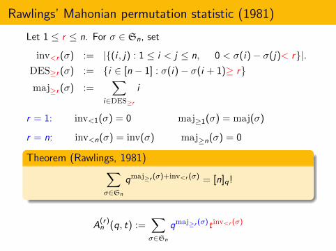
Rawlings’ Mahonian permutation statistic (1981)
Let 1 ≤ r ≤ n. For σ ∈ Sn, set
inv<r (σ) := |{(i , j) : 1 ≤ i < j ≤ n, 0 < σ(i)− σ(j)< r}|.DES≥r (σ) := {i ∈ [n − 1] : σ(i)− σ(i + 1)≥ r}maj≥r (σ) :=
∑i∈DES≥r
i
r = 1: inv<1(σ) = 0 maj≥1(σ) = maj(σ)
r = n: inv<n(σ) = inv(σ) maj≥n(σ) = 0
Theorem (Rawlings, 1981)∑σ∈Sn
qmaj≥r (σ)+inv<r (σ) = [n]q!
A(r)n (q, t) :=
∑σ∈Sn
qmaj≥r (σ)t inv<r (σ)
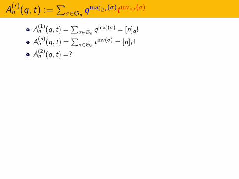
A(r)n (q, t) :=
∑σ∈Sn
qmaj≥r (σ)t inv<r (σ)
A(1)n (q, t) =
∑σ∈Sn
qmaj(σ) = [n]q!
A(n)n (q, t) =
∑σ∈Sn
t inv(σ) = [n]t !
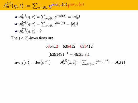
A(2)n (q, t) =?
The (< 2)-inversions are
635412 635412 635412
(635142)−1 = 46.25.3.1
inv<2(σ) = des(σ−1) A(2)n (1, t) =
∑σ∈Sn
tdes(σ−1) = An(t)
Theorem (Shareshian and MW)
A(2)n (q, t) = An(q, t)
Proof involves Stanley’s theory of P-partitions, Gessel’s theory ofquasisymmetric functions, our Eulerian quasisymmetric functions.

A(r)n (q, t) :=
∑σ∈Sn
qmaj≥r (σ)t inv<r (σ)
A(1)n (q, t) =
∑σ∈Sn
qmaj(σ) = [n]q!
A(n)n (q, t) =
∑σ∈Sn
t inv(σ) = [n]t !
A(2)n (q, t) =?
The (< 2)-inversions are
635412 635412 635412
(635142)−1 = 46.25.3.1
inv<2(σ) = des(σ−1) A(2)n (1, t) =
∑σ∈Sn
tdes(σ−1) = An(t)
Theorem (Shareshian and MW)
A(2)n (q, t) = An(q, t)
Proof involves Stanley’s theory of P-partitions, Gessel’s theory ofquasisymmetric functions, our Eulerian quasisymmetric functions.
A(r)n (q, t) :=
∑σ∈Sn
qmaj≥r (σ)t inv<r (σ)
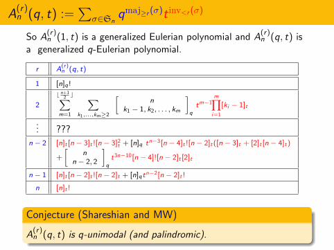
So A(r)n (1, t) is a generalized Eulerian polynomial and A
(r)n (q, t) is
a generalized q-Eulerian polynomial.
r A(r)n (q, t)
1 [n]q!
2
b n+12c∑
m=1
∑k1,...,km≥2
[n
k1 − 1, k2, . . . , km
]q
tm−1m∏i=1
[ki − 1]t
... ???
n − 2 [n]t [n − 3]t ![n − 3]2t + [n]q tn−3[n − 4]t ![n − 2]t([n − 3]t + [2]t [n − 4]t)
+
[n
n − 2, 2
]q
t3n−10[n − 4]![n − 2]t [2]t
n − 1 [n]t [n − 2]t ![n − 2]t + [n]qtn−2[n − 2]t !
n [n]t !
Conjecture (Shareshian and MW)
A(r)n (q, t) is q-unimodal (and palindromic).
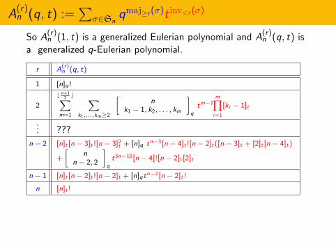
A(r)n (q, t) :=
∑σ∈Sn
qmaj≥r (σ)t inv<r (σ)
So A(r)n (1, t) is a generalized Eulerian polynomial and A
(r)n (q, t) is
a generalized q-Eulerian polynomial.
r A(r)n (q, t)
1 [n]q!
2
b n+12c∑
m=1
∑k1,...,km≥2
[n
k1 − 1, k2, . . . , km
]q
tm−1m∏i=1
[ki − 1]t
... ???
n − 2 [n]t [n − 3]t ![n − 3]2t + [n]q tn−3[n − 4]t ![n − 2]t([n − 3]t + [2]t [n − 4]t)
+
[n
n − 2, 2
]q
t3n−10[n − 4]![n − 2]t [2]t
n − 1 [n]t [n − 2]t ![n − 2]t + [n]qtn−2[n − 2]t !
n [n]t !
Conjecture (Shareshian and MW)
A(r)n (q, t) is q-unimodal (and palindromic).
A(r)n (q, t) :=
∑σ∈Sn
qmaj≥r (σ)t inv<r (σ)
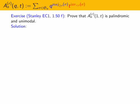
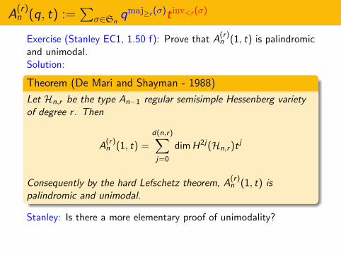
Exercise (Stanley EC1, 1.50 f): Prove that A(r)n (1, t) is palindromic
and unimodal.Solution:
Theorem (De Mari and Shayman - 1988)
Let Hn,r be the type An−1 regular semisimple Hessenberg varietyof degree r . Then
A(r)n (1, t) =
d(n,r)∑j=0
dimH2j(Hn,r )t j
Consequently by the hard Lefschetz theorem, A(r)n (1, t) is
palindromic and unimodal.
Stanley: Is there a more elementary proof of unimodality?Shareshian and MW: Is there a q-analog of this result?(Hn,2 is the toric variety V∆n)
A(r)n (q, t) :=
∑σ∈Sn
qmaj≥r (σ)t inv<r (σ)
Exercise (Stanley EC1, 1.50 f): Prove that A(r)n (1, t) is palindromic
and unimodal.Solution:
Theorem (De Mari and Shayman - 1988)
Let Hn,r be the type An−1 regular semisimple Hessenberg varietyof degree r . Then
A(r)n (1, t) =
d(n,r)∑j=0
dimH2j(Hn,r )t j
Consequently by the hard Lefschetz theorem, A(r)n (1, t) is
palindromic and unimodal.
Stanley: Is there a more elementary proof of unimodality?
Shareshian and MW: Is there a q-analog of this result?(Hn,2 is the toric variety V∆n)

A(r)n (q, t) :=
∑σ∈Sn
qmaj≥r (σ)t inv<r (σ)
Exercise (Stanley EC1, 1.50 f): Prove that A(r)n (1, t) is palindromic
and unimodal.Solution:
Theorem (De Mari and Shayman - 1988)
Let Hn,r be the type An−1 regular semisimple Hessenberg varietyof degree r . Then
A(r)n (1, t) =
d(n,r)∑j=0
dimH2j(Hn,r )t j
Consequently by the hard Lefschetz theorem, A(r)n (1, t) is
palindromic and unimodal.
Stanley: Is there a more elementary proof of unimodality?Shareshian and MW: Is there a q-analog of this result?(Hn,2 is the toric variety V∆n)
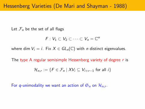
Hessenberg Varieties (De Mari and Shayman - 1988)
Let Fn be the set of all flags
F : V1 ⊂ V2 ⊂ · · · ⊂ Vn = Cn
where dimVi = i . Fix X ∈ GLn(C) with n distinct eigenvalues.
The type A regular semisimple Hessenberg variety of degree r is
Hn,r := {F ∈ Fn | XVi ⊆ Vi+r−1 for all i}
For q-unimodality we want an action of Sn on Hn,r .

The Representation
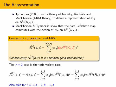
Tymoczko (2008) used a theory of Goresky, Kottwitz andMacPherson (GKM theory) to define a representation of Sn
on H2j(Hn,r ).MacPherson & Tymoczko show that the hard Lefschetz mapcommutes with the action of Sn on H2j(Hn,r ) .
Conjecture (Shareshian and MW)
A(r)n (q, t) =
d(n,r)∑j=0
psq(chH2j(Hn,r ))t j
Consequently A(r)n (q, t) is q-unimodal (and palindromic).
The r = 2 case is the toric variety case.
A(2)n (q, t) = An(q, t) =
n−1∑j=0
psq(chH2j(V∆n))t j =n−1∑j=0
psq(chH2j(Hn,2))t j
Also true for r = 1, n − 2, n − 1, n
The Representation
Tymoczko (2008) used a theory of Goresky, Kottwitz andMacPherson (GKM theory) to define a representation of Sn
on H2j(Hn,r ).MacPherson & Tymoczko show that the hard Lefschetz mapcommutes with the action of Sn on H2j(Hn,r ) .
Conjecture (Shareshian and MW)
A(r)n (q, t) =
d(n,r)∑j=0
psq(chH2j(Hn,r ))t j
Consequently A(r)n (q, t) is q-unimodal (and palindromic).
The r = 2 case is the toric variety case.
A(2)n (q, t) = An(q, t) =
n−1∑j=0
psq(chH2j(V∆n))t j =n−1∑j=0
psq(chH2j(Hn,2))t j
Also true for r = 1, n − 2, n − 1, n
Chromatic symmetric functions
1
23
4
5
67 8
Wednesday, December 7, 2011
1
23
4
5
67 8
77
15 15
23
23
23
35
23
23
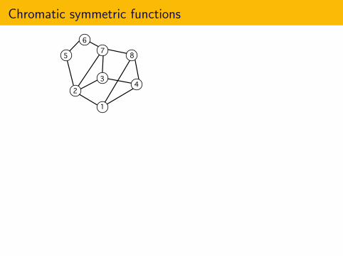
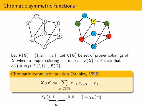
Let V (G ) = {1, 2, . . . , n}. Let C (G ) be set of proper colorings ofG , where a proper coloring is a map c : V (G )→ P such thatc(i) 6= c(j) if {i , j} ∈ E (G ).
Chromatic symmetric function (Stanley, 1995)
XG (x) :=∑
c∈C(G)
xc(1)xc(2) . . . xc(n)
XG (1, 1, . . . , 1︸ ︷︷ ︸, 0, 0, . . . ) = χG (m)
m
Chromatic symmetric functions
1
23
4
5
67 8
1
23
4
5
67 8
77
15 15
23
23
23
35
23
23
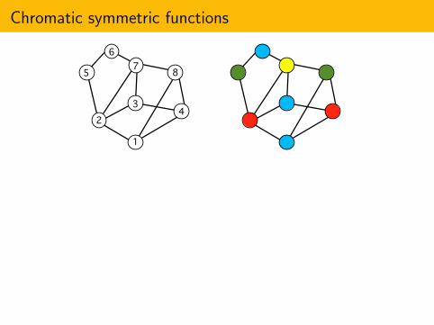
Let V (G ) = {1, 2, . . . , n}. Let C (G ) be set of proper colorings ofG , where a proper coloring is a map c : V (G )→ P such thatc(i) 6= c(j) if {i , j} ∈ E (G ).
Chromatic symmetric function (Stanley, 1995)
XG (x) :=∑
c∈C(G)
xc(1)xc(2) . . . xc(n)
XG (1, 1, . . . , 1︸ ︷︷ ︸, 0, 0, . . . ) = χG (m)
m

Chromatic symmetric functions
1
23
4
5
67 8
77
15 15
23
23
23
35
23
23
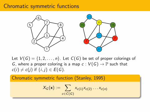
Let V (G ) = {1, 2, . . . , n}. Let C (G ) be set of proper colorings ofG , where a proper coloring is a map c : V (G )→ P such thatc(i) 6= c(j) if {i , j} ∈ E (G ).
Chromatic symmetric function (Stanley, 1995)
XG (x) :=∑
c∈C(G)
xc(1)xc(2) . . . xc(n)
XG (1, 1, . . . , 1︸ ︷︷ ︸, 0, 0, . . . ) = χG (m)
m
Chromatic symmetric functions
1
23
4
5
67 8
77
15 15
23
23
23
35
23
23
Let V (G ) = {1, 2, . . . , n}. Let C (G ) be set of proper colorings ofG , where a proper coloring is a map c : V (G )→ P such thatc(i) 6= c(j) if {i , j} ∈ E (G ).
Chromatic symmetric function (Stanley, 1995)
XG (x) :=∑
c∈C(G)
xc(1)xc(2) . . . xc(n)
XG (1, 1, . . . , 1︸ ︷︷ ︸, 0, 0, . . . ) = χG (m)
m
Chromatic quasisymmetric function
1
23
4
5
67 8
77
15 15
23
23
23
35
23
23
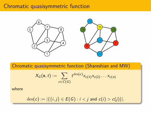
Chromatic quasisymmetric function (Shareshian and MW)
XG (x, t) :=∑
c∈C(G)
tdes(c)xc(1)xc(2) . . . xc(n)
where
des(c) := |{{i , j} ∈ E (G ) : i < j and c(i) > c(j)}|.
Chromatic quasisymmetric function
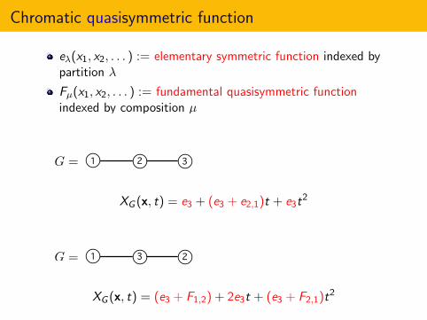
eλ(x1, x2, . . . ) := elementary symmetric function indexed bypartition λ
Fµ(x1, x2, . . . ) := fundamental quasisymmetric functionindexed by composition µ
1 2 3G =
XG (x, t) = e3 + (e3 + e2,1)t + e3t2
1 3 2G =
XG (x, t) = (e3 + F1,2) + 2e3t + (e3 + F2,1)t2
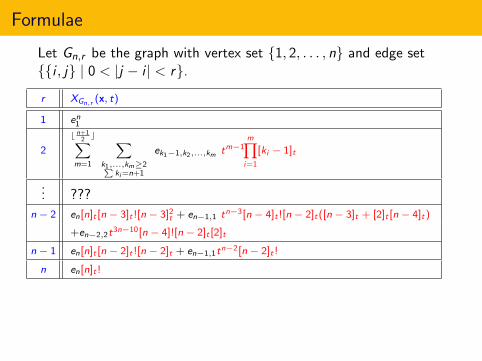
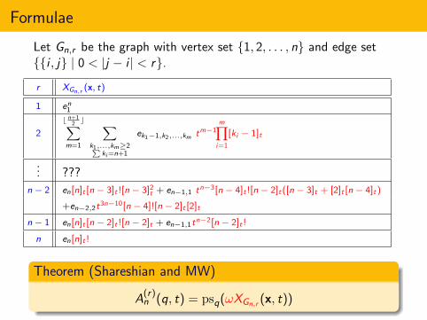
Formulae
Let Gn,r be the graph with vertex set {1, 2, . . . , n} and edge set{{i , j} | 0 < |j − i | < r}.
r XGn,r (x, t)
1 en1
2
b n+12c∑
m=1
∑k1,...,km≥2∑
ki=n+1
ek1−1,k2,...,km tm−1m∏i=1
[ki − 1]t
... ???
n − 2 en[n]t [n − 3]t ![n − 3]2t + en−1,1 tn−3[n − 4]t ![n − 2]t([n − 3]t + [2]t [n − 4]t)
+en−2,2t3n−10[n − 4]![n − 2]t [2]t
n − 1 en[n]t [n − 2]t ![n − 2]t + en−1,1tn−2[n − 2]t !
n en[n]t !
Theorem (Shareshian and MW)
A(r)n (q, t) = psq(ωXGn,r (x, t))

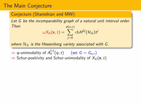
The Main Conjecture
Conjecture (Shareshian and MW)
Let G be the incomparability graph of a natural unit interval order.Then
ωXG (x, t) =
d(n,r)∑j=0
chH2j(HG )t j
where HG is the Hessenberg variety associated with G .
⇒ q-unimodality of A(r)n (q, t) (set G = Gn,r )
⇒ Schur-positivity and Schur-unimodality of XG (x, t)
Theorem (Shareshian and MW - t-analog of Gasharov)
Let G be the incomparability graph of a natural unit interval orderP. Then
XG (x, t) =∑T∈TP
t invG (T )sλ(T ),
where TP is the set of P-tableaux, invG is an inversion statistic ontableaux, and λ(T ) is the shape of T .
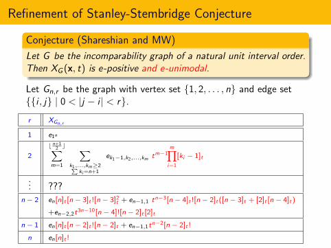
Refinement of Stanley-Stembridge Conjecture
Conjecture (Shareshian and MW)
Let G be the incomparability graph of a natural unit interval order.Then XG (x, t) is e-positive and e-unimodal.
Let Gn,r be the graph with vertex set {1, 2, . . . , n} and edge set{{i , j} | 0 < |j − i | < r}.
r XGn,r
1 e1n
2
b n+12c∑
m=1
∑k1,...,km≥2∑
ki=n+1
ek1−1,k2,...,km tm−1m∏i=1
[ki − 1]t
... ???
n − 2 en[n]t [n − 3]t ![n − 3]2t + en−1,1 tn−3[n − 4]t ![n − 2]t([n − 3]t + [2]t [n − 4]t)
+en−2,2t3n−10[n − 4]![n − 2]t [2]t
n − 1 en[n]t [n − 2]t ![n − 2]t + en−1,1tn−2[n − 2]t !
n en[n]t !


![Author's personal copy · 2011. 4. 3. · quasisymmetric functions and other key terms can be found in Section 2. Shareshian and Wachs [15,16] derive a formula for the generating](https://img.pdfslide.us/doc/110x75/60f80043ee12f42d3a01338a/authors-personal-copy-2011-4-3-quasisymmetric-functions-and-other-key-terms.jpg)