NBER WORKING PAPER SERIES

ADJUSTMENT AND STRUCTURAL CHANGEUNDER SUPPLY SHOCKS

Michael Bruno

Working Paper No. 8114

NATIONAL BUREAU OF ECONOMIC RESEARCH1050 Massachusetts Avenue

Cambridge MA 02138

December 1981

The research reported here is part of the NBER's research programin International Studies. Any opinions expressed are those of theauthor and not those of the National Bureau of Economic Research.

NBER Working Paper #814December 1981

ADJUSTMENT AND STRUCTURAL CHANGE UNDER SUPPLY SHOCKS

ABSTRACT

The resource boom effect and the input price effect of

raw material price changes are analyzed within a two—period,

two-sector (plus resource industry), open economy framework.

Diagrammatic exposition is used to study the 'dutch disease',

and in particular the distinction between the short term wealth

effects (causing a real appreciation and a movement of variable

factors from tradable to non—tradable industries) and between

the long—run effects on total investment, its sectoral allocation

and its finance by foreign borrowing. The framework further

enables analysis of the different allocational effects of tem-

porary versus permanent raw material price increases, when the

two sectors differ in material use. Also discussed are the

effects of changes in the world interest rate on factor allocation

and foreign borrowing as well as the allocational effects of

government intervention in the case of temporary real wage

rigidity.

Michael BrunoDepartment of EconomicsHebrew UniversityJerusalem, Israel

Tel. (2)—6360l5

ADJUSTMENT AND STRUCTURAL CHANGE

UNDER SUPPLY SHOCKS

I ntroduction*

Macro—economic adjustment and long—term structural changes are

often closely related, yet they are usually kept in separate analy-

tical boxes. Nowhere is the inadequacy of such dichotomy more ap-

parent than in the understanding of the developments and policy

response of individual countries after the supply shocks of the 1970s.

Raw materials price increases played a major role in the ensuing

stagflation, which could be perceived as a short—term macro—economic

adjustment problem. However, as time progressed it became more

and more clear that the longer run implications of these shocks

on productivity and profitability are at least as important.

There are two different aspects of raw material price effects

which have been discussed under separate headings. One is the

resource boom effect (see, for example, Corden and Neary (1980)).

If a country is a net exporter of a raw material whose price has

increased, there will be a short run increase in the relative price

of non—tradable goods (or a real appreciation) and a shift in var-

iable factors out of existing tradable goods such as manufacturing,

say, and into services. Relative profitability will further affect

* This paper is part of a project on Structural Adjustment in OpenEconomies conducted together with Jeffrey Sachs at the NationalBureau for Economic Research in Cambridge, Mass. and at the FalkInstitute for Economic Research, Jerusalem. Financial supportby the National Science Foundation and the Ford Foundation isgratefully acknowledged.

I have benefitted from discussions with Jeffrey Sachs in thepreparation of this paper. Likewise, I am indebted to LarsSvensson, Lars Caimfors, and other participants at the 1981SaltsjObaden conference for helpful comments on an earlier draft.Svensson has independently worked out several of the propositionsanalyzed here (see Svensson (1981)).

2

today's investment and therefore future production and capital

in place in the various sectors. It is important to stress,

however, that this is only one example of a pure wealth effect,

which could also take place when an oil discovery is announced

or, in a completely different context, when a country receives

an unexpected foreign currency transfer (much like the old

"transfer problem"). The analysis of this type of problem is

best conceived in a framework in which international capital

mobility is allowed for, because a wealth change will affect the

country 's borrowing.

Another, probably more important, aspect is that of the role

of raw materials as a major input into the productive system. This

may hit both net importers as well as net exporters of such material

and would tend to shift resources away from a raw material intensive

activity into less-intensive ones. This, too, might cause "de-

industrialization" but for a different reason. In this context,

it is important to make the distinction between temporary and per-

manent change in raw material prices. The former may have wealth

effects but need not cause long—run changes in relative prices.

It is mainly the latter that will affect investment behavior.

The present paper extends an earlier factor—price—frontier

analysis of mine (1981) to a two-sector framework (sections I and II)

It then analyzes the above issues in a two—period dynamic framework

which is a stripped down version of a model that was previously

used for simulation experiments (Sachs (1980), Bruno and Sachs (l981)).l

1 Louis Dicks-Mireaux is presently applying a similar framework forthe U.K.

3

After laying out the ingredients of the model in terms of pro-

duction (II), household behaviour (III), investment and the current

account (IV), diagrammatic exposition is used to show the effects

of pure wealth and public expenditure changes (V), temporary and

permanent change in raw material prices (VI) as well as the effect

of changes in world interest rates and alternative current account

objectives (VII) . The paper ends with a brief discussion of the

effect of short-term real wage rigidity and the related policy

response.

I. The factor-price-frontier, raw material prices and dynamic

adjustment

The effect of raw material prices on the supply side of an

open economy is best illustrated within the framework of the factor

price frontier, in a three factor production world, which will here

be reiterated only in summary form. Assume first that the economy

consists of a single sector and let Q = Q(L,K,N) be a well-behaved

constant returns production function for gross output of a final

good using labour, L, capital, K, and a raw material, N. The price

of the output is P, and that of the raw material is P. For the

time being assume that the relative price ll = Ps/P is given (as is

the case if both N and Q are tradeable goods in a small open economy).

Let Y be the real income derived, Y = Q — llN1 and assume optimal

use of N such that Q/N = 11n Denote the real returns (marginal

products) to labour and capital by and R respectively.

The factor-price frontier (FFP) summarizes the information about

the technology in terms of the maximal combinations of the three

marginal factor products, (WRIH) = 0. The curve is drawn in

4

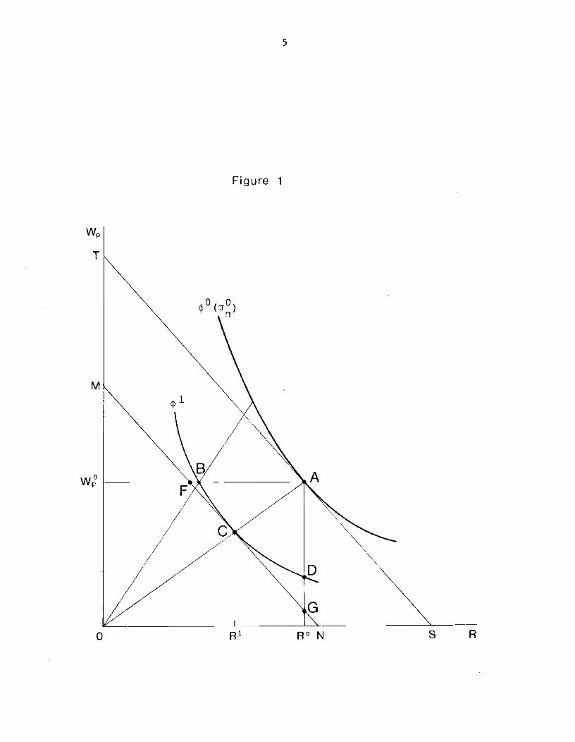
W — R space (see Figure 1) for a given relative raw—material price

1101s downward sloping and convex to the origin. The slope of

the tangent at the point A measures the capital/labour ratio that

corresponds to the pair of factor prices (R°W° ) and its intercept

on the Waxis (OT) measures Y/L. Likewise the intercept on the R

axis (OS) measures Y/K. The elasticity of FPF at the point A = SA/TA

measures the relative shares of capital and labour in Y.

Weak separability of the production function which will be

assumed here {Q = Q[V(L,K), N]} implies weak separability

of the dual FPF, i.e., will take the form {f(W,R), ll] = 0.

A raw—material price increase, like Hicks-neutral technical regress,

is represented by a homothetic inward shift of the FPF from to '

Only at the point C on the new FPF, on a ray OA, will the capital/

labour ratio be the same as at A. C is thus a full-employment point,

in the short run (when K = K, L = L) . Both real factor rewards at C

must fall at the same rate from their original level at A. Total

real income per unit of labour (Y/L) likewise falls by the same

proportion from OT to OM (and Y/K from OS to ON). The case of real

wage rigidity at W0, which may occur in the very short run, is

represented by the point B where R and Y/K must of necessity fall by

more than at C and the capital/ labour ratio is higher than at C.

At the initial/capital stock K, L must fall and unemployment will

1emerge, as long as the real wage does not fall by the required amount.

11n the putty-clay case in which the capital/labour ratio cannotimmediately adjust to the new factor prices, the various solutions aregiven along the line FCG, i.e. in the rigid real wage, rigid capital/labour ratio case the economy will be at F and not at B, the rate ofprofit falling by more than at B, and L staying constant.

One should also point out that under an alternative technologicalassumption the FPF need not shift honDthetically . See Bruno (1981)for a more detailed discussion.

wp

I

M

wpo

5

Figure 1

0 R' R°N S R

q0 ('if0)

A

6

The polar case to the very short run (W = W) is that of an

imposed long—run real rate of return (R = R°). This is represented

by the point D, to be termed the long-run, at which the real wage

and the capital/labour ratio are below their levels at C. In

contrast to C, the point D may represent an equilibrium steady—

state level after capital has adjusted downward to a given real

rate of return, R0. With full employment of labour, capital and

output (gross and net) at D must both lower than at the initial

point A.

To see the short—run and long—run implications of a permanent

raw material price shock within this framework one may consider

some simple dynamics in terms of two key variables, the real

wage and the capital stock. The real wage can be made to change

as a function of unemployment, in Phillips curve fashion. The

capital stock can be made to adjust via an investment function

that will depend in some measure on the instantaneous and future

expected profit rate. With the aid of such a two-equation dynamic

model, one can analyze the alternative paths leading to an

ultimate steady state at the point D.1 An alternate procedure,

which we shall adopt in the more detailed two-sector discussion

below, is to think of the horizon as consisting of two periods,

1One has to keep in mind that a growing economy will usually also

exhibit pure technical progress. To avoid the need to have the FPFsimultaneously shift outward, when there is technical progress, onemay instead redefine factor products to be measured in intensity units.Thus in the empirically relevant case of Harrod neutral (or labouraugmenting) technical progess, for example, the real wage (Wv) must bereinterpreted as being measured relative to its long run trend.Another implication of this is that when we talk of a fall incapital—labour ratios what may be implied is only a fall relativeto what it would be in the absence of the exogenous shock.

7

the short run, in which the capital stock is fixed, and the second

period, the long run, for which first period investment may affect

long-run capital in place. In this way today's investment is

uniquely determined by the expected future rate of profit, which

in turn depends on the assumptions made about future factor prices

and the extent of international capital mobility.

II. A two-period model of production and factor allocation

There are a number of interesting issue, relating to the

role of raw materials, which are of necessity ignored when one

looks at a single sector economy.1 Demand has so far played no

role at all. Also there was no role for endogenous changes in

relative commodity prices leading to compositional shifts within

the economy. In the context of the role of raw materials composi-

tional shifts , be of great importance in more than one respect.

A mineral boom leads to the so-called 'dutch disease', whereby

an existing tradable goods industry may be squeezed out by real

appreciation of the exchange rate, while a domestic service industry

may expand (see Corden and Neary (1981), Neary and Purvis (1981)

and van Wijnbergen (1981)) . A more direct effect of a rise in the

price of raw materials might be to contract the industry that is

relatively intensive in raw material use while a less raw material

intensive industry might contract less or even expand.2

1The single sector formulation can, however, be usefully applied tothe empirical analysis of a single large tradable goods sector suchas manufacturing.

21f the country is a producer of both the raw material and the rawmaterial using final tradable goods, such as most manufactures, de—industrialization may thus occur for a combination of both reasons, asis the case in the U.K., for example.

8

In the case of both phenomer..a it is important to distinguish between

short—run and long-run effects of the exogenous changes that are

taking place. In the short run only variable factors (e.g. labour)

may be free to move from one sector into the other (If real wages

are rigid there may also be room for government intervention)

Relative profitability changes may, however, induce long—run changes

in capital investment patterns. Whether the latter will in fact

take place in turn depends on the extent to which the exogenous

changes (e.g. in mineral prices) are perceived to be temporary or

permanent. All of these considerations lead to the choice of a

multisectoral as well as inter—temporal framework of analysis.

A natural extention of the model briefly discussed in the

previous section would be one in which another non—tradeable goods

sector is added on, in true Scandinavian tradition. Its extention

to an infinite horizon framework becomes analytically intractable, as

the number of state variables jumps to three or more. One way out

is to run computer simulations of such models which can be made as

complex as one wishes (see Sachs, (1980), Bruno and Sachs (1981)).

Useful as these are, they do, however, have the drawback that it is

often hard to see through how particular results depend on specific

numerical assumptions made.

To obtain relative analytical simplicity we shall here sacrifice

the full fledged long-term horizon. Much of what is relevant in the

distinction between the short and the long-run can be seen from

looking at two—period simplifications of the world. Even a rational

expectations view of investment, based on future prices, can be

9

expressed in this way, without need to bring in explicitly

Tobin's q or the 'costs of adjustment.' Finally the view of

the balance of payments in its interternporal allocation aspects

can be fitted well into this scheme.1

Consider a two—commodity framework, tradeables (or the

'foreign' sector with subscript f) and domestic non-tradeables

(with subscript d) within a two-period horizon (using superscript

t = 1,2).Production of tradeables Qf = Qf(Lf? Kf , N) uses inputs of

labour (Lf). fixed initial capital (Kf) and raw materials (N)? it

supplies the demand for private consumer goods (Cf) investment

goods (I) and net exports (X) . The latter may be negative (net

imports). The domestic price of tradeables equals the world

price (p*) times the exchange rate (e). The noi—tradeable goods

sector will be assumed to use only labour and capital, d = d'd' Kd)

and to supply only private (Cd) and public (G) consumer goods. The

respective sector specialization in the production of exports,

investment goods and public consumption and in the use of raw

materials is not essential but clearly simplifies the analysis.

There is a third sector in the economy, producing a fixed quantity

of tradeable raw materials (H1, H2), for which the fixed inputs

will not be separately accounted. The country may be a net

'A mu1tictOral,intertemporal, view of foreign trade and investmentallocation was very popular in the Trade and Develooment literatureof the 1960's, mostly based on empirical development proqrammincrmodels, but also including some theoretical contributions see e.g.Bardhan (1966), Bruno (1967) . However, the associated short-termadjustment problem was usually discussed in a separate box. Forrecent two—period formulations of investment and the balance ofpayments see Razin (1980), Sachs (1981).

2 i 1We shall assume separability Q4, = QçtVç(Lf Kf)l N -' as before, aswell as constant returns.

10

importer or net exporter of raw materials which command a given

world price p.

While the total labour supply is fixed in both periods

t t _t(Ld + Lf = L ) capital in each sector in the second period is

augmented or contracted by the amount of tradeable investment

goods produced (or traded) for each sector in the first period

(K - Kd + K - = Ii). For simplicity we assume no depreciation

but allow for negative I No new investment goods have to be

produced in the second period since this represents the along—run

with K, K staying on for posterity.

The main distinction between the two periods is that in

the first, the short-run, capital is held fixed and is sector-

specific, while in the second, the long—run, it is malleable.

On the production side this model has its antecedents in the

work of Mayer (1974) and others. The earlier model is here

extended to take into account investment and wealth as well as

the role of raw materials.

Production and factor rewards are obtained from firm

maximization of discounted cash flow. If the relative price of

domestic over foreign goods is denoted by r= d'f'1 that of

raw materials by irs, the real wage in foreign good units is Wf

and the own rate of interest on foreign goods is r, firms

maximize (Q + TF'Q - wL' -TrN1

— I') + (l+r) l( Q + IT2Qd2_W2L2_.1F2N2)

subject to the labour and production constraints. The usual first

order conditions are obtained for both periods:

1The reciprocal of = e.p*/pd) is often termed thereal exchange rate.

11

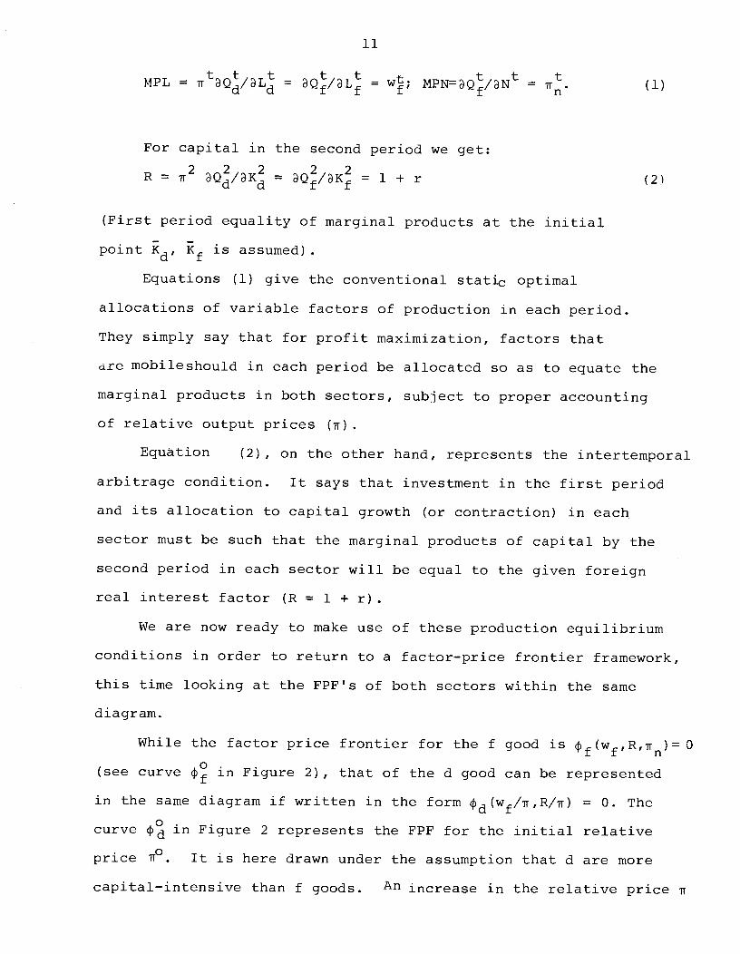
MPL = tQt/Lt = = w; MPNQ/aNt = (1)

For capital in the second period we get:

R = 2 = = 1 + r (2)

(First period equality of marginal products at the initial

point Kd, Kf is assumed).

Equations (1) give the conventional static optimal

allocations of variable factors of production in each period.

They simply say that for profit maximization, factors that

are mobileshould in each period be allocated so as to equate the

marginal products in both sectors, subject to proper accounting

of relative output prices (ii)

Equation (2), on the other hand, represents the intertemporal

arbitrage condition. It says that investment in the first period

and its allocation to capital growth (or contraction) in each

sector must be such that the marginal products of capital by the

second period in each sector will be equal to the given foreign

real interest factor (R = 1 + r).

We are now ready to make use of these production equilibrium

conditions in order to return to a factor—price frontier framework,

this time looking at the FPF's of both sectors within the same

diagram.

While the factor price frontier for the f good is4f (wfFR7r = 0

(see curve in Figure 2), that of the d good can be represented

in the same diagram if written in the form d(wf/Tr,R/rr) = 0. The

curve in Figure 2 represents the FPF for the initial relative

price iT°. It is here drawn under the assumption that d are more

capital—intensive than f goods. An increase in the relative price rr

Wf

12

Figure 2

w

R°2Q2/K2

R

13

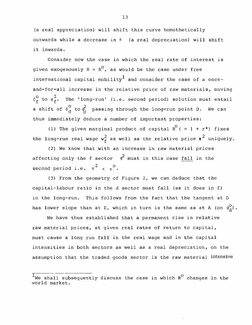
(a real appreciation) will shift this curve homothetically

outwards while a decrease in 'ii (a real depreciation) will shift

it inwards.

Consider now the case in which the real rate of interest is

given exogenously R = R0, as would be the case under free

international capital mobility1 and consider the case of a once—

and—for—all increase in the relative price of raw materials, moving

to . The 'long-run' (i.e. second period) solution must entail

a snift of to passing through the long-run point D. We can

thus immediately deduce a number of important properties:

(1) The given marginal product of capital R°( = 1 + r*) fixes

2 2the long—run real wage Wf as well as the relative price it uniquely.

(2) We know that with an increase in raw material prices

affecting only the f sector 'rr2 must in this case fall in the

second period i.e. <

(3) From the geometry of Figure 2, we can deduce that the

capital—labour ratio in the d sector must fall (as it does in f)

in the long-run. This follows from the fact that the tangent at D

has lower slope than at E, which in turn is the same as at A (on

We have thus established that a permanent rise in relative

raw material prices, at given real rates of return to capital,

must cause a long run fall in the real wage and in the capital

intensities in both sectors as well as a real depreciation, on the

assumption that the traded goods sector is the raw material intensive

'We shall subsequently discuss the case in which R° changes in theworld market.

14

industry. What is left open is the composition of output

Here demand must naturally play an important role.

III. Consumption, wealth and short-run equilibrium.

We shall assume that households decide on their consumption

basket by maximizing discounted utility subject to a given net/

wealth constraint:

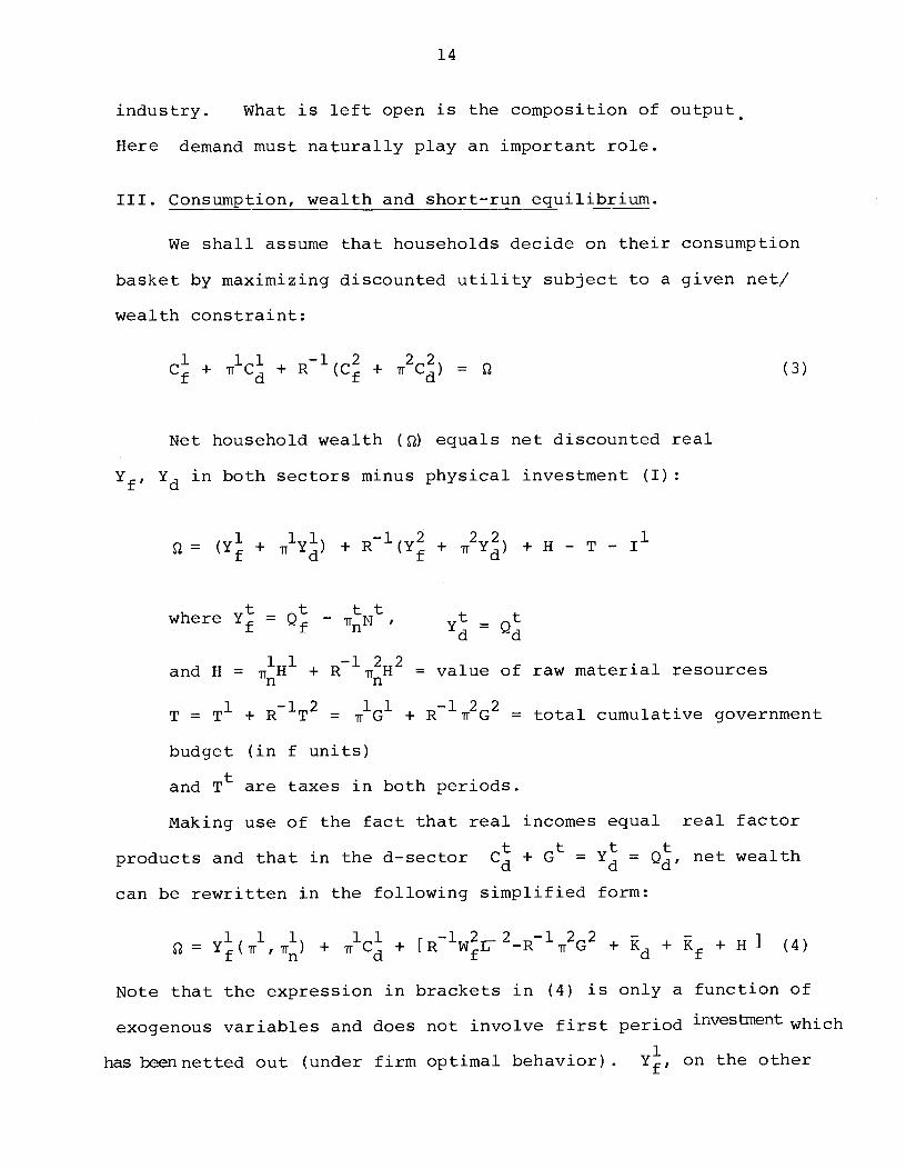
C + iIC + R1(C + ir2C) = (3)

Net household wealth (Q) equals net discounted real

Yf Y in both sectors minus physical investment (I):

= (Y + ir1Y) + R1(Y + ir2Y) + H - T -

t t ttwhereYf=Qf-TN ytQtd d

and H = H' + R1ir2H2 = value of raw material resources

1 —12 11 —122T = T + R P = G + B ir G = total cumulative government

budget (in f units)

tand T are taxes in both periods.

Making use of the fact that real incomes equal real factor

products and that in the d-sector C + Gt = = Q, net wealth

can be rewritten in the following simplified form:

Q = Y(ir11ir1) + ir1C + [R1WE2Rr2G2 + Kd + Kf + H] (4)

Note that the expression in brackets in (4) is only a function of

exogenous variables and does not involve first period investment which

has been netted out (under firm optimal behavior). on the other

15

hand, can be expressed as a function of the relevant first period

variables.

In the case of a flexible labour market, with which we shall

deal most of the time, first period's net output of tradeables1 1 11 1

(Yf=

Qf— •itN ) can be written as a negative function of ii

which equals the marginal rate of substitution on the short—run

production possibility curve. It will also be a negative function

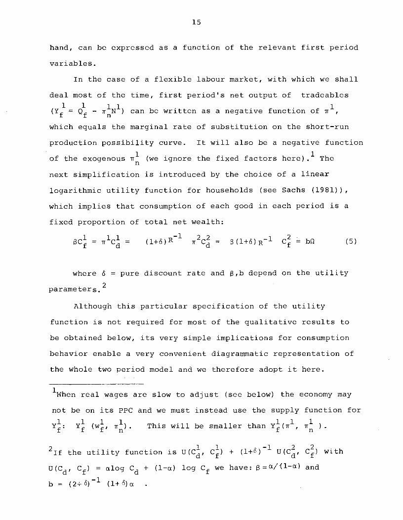
of the exogenous (we ignore the fixed factors here).1 The

next simplification is introduced by the choice of a linear

logarithmic utility function for households (see Sachs (1981))

which implies that consumption of each good in each period is a

fixed proportion of total net wealth:

= r1C = (l+6)1 = (l+)R' C bQ (5)

where ó = pure discount rate and ,b depend on the utility

parameters.2

Although this particular specification of the utility

function is not required for most of the qualitative results to

be obtained below, its very simple implications for consumption

behavior enable a very convenient diagrammatic representation of

the whole two period model and we therefore adopt it here.

'When real wages are slow to adjust (see below) the economy may

not be on its PPC and we must instead use the supply function for

Y: Y (w, .111). This will be smaller than Y(ir1, ii ).

2 1 1 -—1 2 2If the utility function is U(Cai Cf) + (1+O) U(Cd? Cf) with

U(Cdl Cf) c1og Cd + (l-c) log Cf we have: =ct/'(1) and

b = (2)1 (l-f)ct .

16

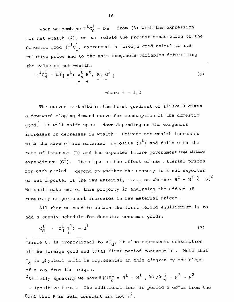
When we combine rr1C = bQ from (5) with the expression

for net wealth (4), we can relate the present consumption of the

domestic good (Tr1C, expressed in foreign good units) to its

relative price and to the main exogenous variables determining

the value of net wealth:

11 1 t t 2Tr

Cd= bQ ir ; rr H , R, G (6)

+ +

where t = 1,2

The curved markedbQ in the first quadrant of figure 3 gives

a downward sloping demand curve for consumption of the domestic

good.1 It will shift up or down depending on the exogenous

increases or decreases in wealth. Private net wealth increases

twith the size of raw material deposits (H ) and falls with the

rate of interest (R) and the expected future government expenditure

expenditure (G2). The signs on the effect of raw material prices

for each period depend on whether the economy is a net exporter

t t> 2or net importer of the raw material, i.e., on whether H - N < 0.

We shall make use of this property in analysing the effect of

temporary or permanent increases in raw material prices.

All that we need to obtain the first period equilibrium is to

add a supply schedule for domestic consumer goods:

C = Q(iT1)- (7)

1.Since Cf is proportional to lrCd, it also represents consumption

of the foreign good and total first period consumption. Note that

Cd in physical units is represented in this diagram by the slope

of a ray from the origin.

2Strictly speaking we have = H' - N1 ,= H2 - N2

- (positive term). The additional term in period 2 comes from the

act that R is held constant and not

17

To conform to the variables in the diagram we multiply both

sides of equation (7) by the relative price ir1. This curve is

upward sloping and shifts down and to the right with increases

1in G

Even before looking at investment and second period equilibrium

we can already deduce that any factor that increases wealth (in

units of the f good) will cause an increase in present consumption

and will also cause a real appreciation in the short run. The

latter in turn implies a shift of labor and production from tradeable

goods to non—tradable goods e.g. from manufacturing into services.

Here is one manifestation of de-industrialization in the short—run.

Note that an increase in wealth may be caused by a variety of

reasons, including the news that a North-Sea oil discovery is

expected in the long-run (i.e. H2rises). Likewise one gets the

usual result that a temporary fiscal expansion (G1 rises but G2

stays constant) crowds out private consumption and causes a real

appreciation, if public expenditure is centered on domestic goods.

More relevant in the present context, however, are the long—run

effects of such expansion. We appropriately turn to investment and

second period equilibrium.

18

Iv. Investment, foreign borrowing and long run production

Having shown how future factor prices and first period

equilibrium are determined all that is left to complete the

solution of the system is to show how the future ccinposition of

output and capital stock are determined. This will tell us what

todayts investment will be which in turn will determine the current

account.

With constant returns to scale, output and labor demands

can be written as proportions of capital stocks in each sector.

Since future relative prices are uniquely determined we can

write the second period supply equation for the domestic

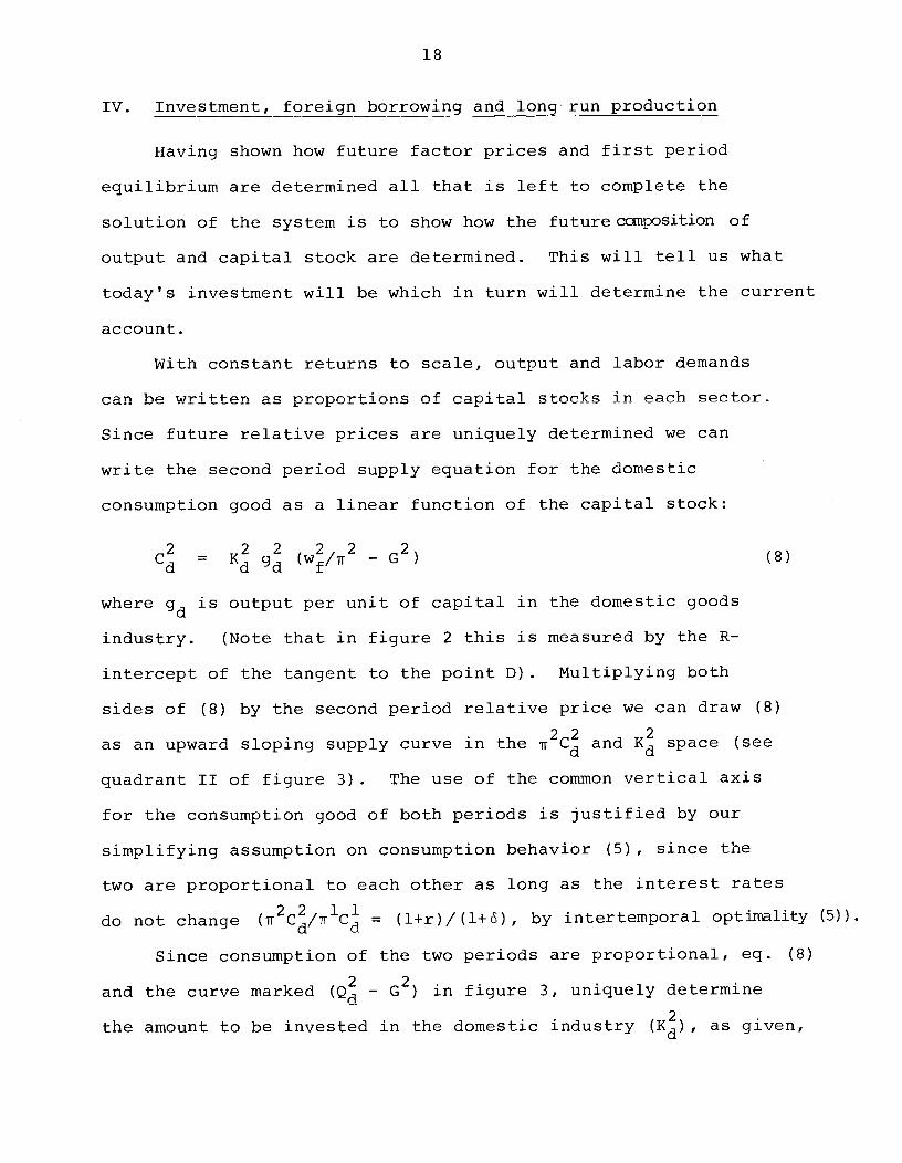
consumption good as a linear function of the capital stock:

2 22 22 2Cd = 'd (Wf/rr - G ) (8)

where is output per unit of capital in the domestic goods

industry. (Note that in figure 2 this is measured by the R-

intercept of the tangent to the point D). Multiplying both

sides of (8) by the second period relative price we can draw (8)

as an upward sloping supply curve in the rr2C and space (see

quadrant II of figure 3) . The use of the common vertical axis

for the consumption good of both periods is justified by our

simplifying assumption on consumption behavior (5), since the

two are proportional to each other as long as the interest rates

do not change N2C/ii1C = (l+r)/(l+S), by intertemporal optimality (5)).

Since consumption of the two periods are proportional, eq. (8)

and the curve marked (Q - G2) in figure 3, uniquely determine

the amount to be invested in the domestic industry (Kg), as given,

19

for example, at the point A2.

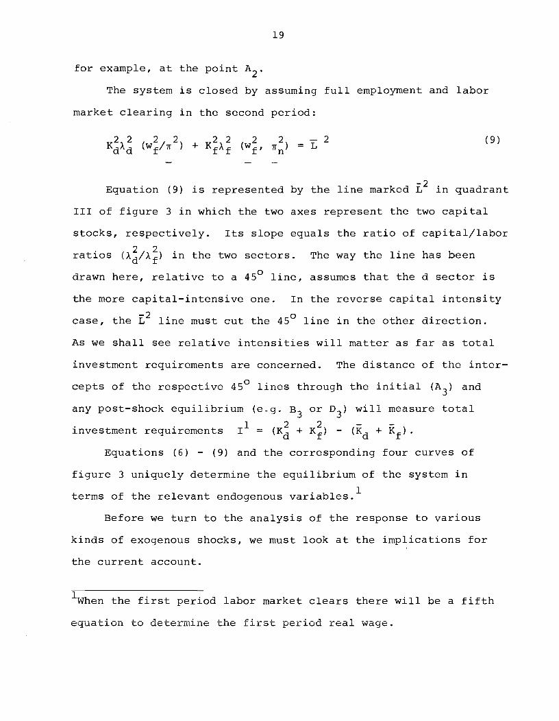
The system is closed by assuming full employment and labor

market clearing in the second period:

22 2 2 22 2 2 —2 (9)KdAd (Wf/lr ) + KfAf (Wf , ) = L

Equation (9) is represented by the line marked L2 in quadrant

III of figure 3 in which the two axes represent the two capital

stocks, respectively. Its slope equals the ratio of capital/labor

ratios (A/X) in the two sectors. The way the line has been

drawn here, relative to a 450 line, assumes that the d sector is

the more capital-intensive one. In the reverse capital intensity

case, the 2 line must cut the 45° line in the other direction.

As we shall see relative intensities will matter as far as total

investment requirements are concerned. The distance of the inter-

cepts of the respective 45° lines through the initial (A3) and

any post-shock equilibrium (e.g. B3 or D3) will measure total1 2 2 — —

investment requirements I = (Kd + Kf) - (Kd + Kf).

Equations (6) — (9) and the corresponding four curves of

figure 3 uniquely determine the equilibrium of the system in

terms of the relevant endogenous variables.1

Before we turn to the analysis of the response to various

kinds of exogenous shocks, we must look at the implications for

the current account.

1When the first period labor market clears there will be a fifth

equation to determine the first period real wage.

20

Figure 3

TI1

22'ft C

22'IT

11'if

Cd

Tr (Q—G1)

\III

\

K2

I

E2

0

22TI C

III

Kd+Kf

Kf

21

The current account in f units (Ft) can be written down as

follows (t = 1, 2):

Ft = - TrtNt + TrtHt - C - = 4 + -Cf

-

where i2 = 0 and C = (1+)'RC by (3).

Note that for each period (Yf + TTnH) is total net production of

foreign exchange (including raw materials) while (Y + it_H - C)I Li

must by deeinition be equal to total domestic savings (S)1, which

is I + F. The line marked in quadrant I of figure 3 describes

+ H1]. Its vertical distance from the line2

(whose co-ordinate is ir Cd = Cf) is proportional to savings in

the first period (S1). The line is of necessity steeper than

so that ceteris paribus S1 falls with ir'. The difference

(S' — Ii) measures the current account surplus (F').

We shall consider two possibilities. One is the case in which

there is no endogenous capital mobility and F1 and F2 are held

equal to zero or to some pre—specified given numbers. The other

case to which we shall turn first is the one in which borrowing and

lending take place at a given world interest rate r*. In this case

we must have R° = (l+r*) and the balance of payments constraint

takes the form

F1 + (l+r*)F2 = 0 (11)

1Another way of seeing this is to note thatS = Yf + ¶H + TFQa - ('rrCd+Cf) - trG = Yf + •TlnH - Cf

since Q = C + G.

This vertical1distance depends on (B-b)Yf( )which is a negativefunction of it since >b.

22

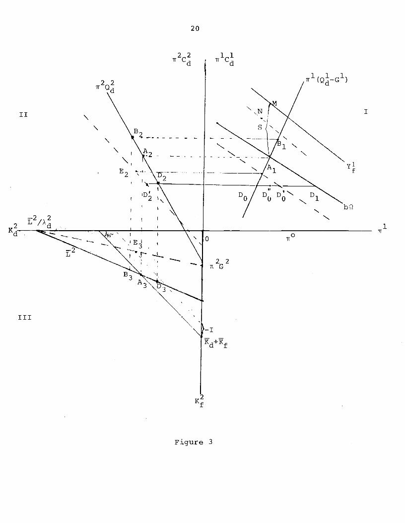
It is readily established that, upon substitution of (10),

equations (11) and (3) become the same budget constraint for

R = l+r*. In fact, the whole pattern of resource allocation and

pricing described above could be got from the solution of an

optimal growth problem in which society is assumed to maximize

discounted utility, as above, subject to the various production

and supply constraints in the two periods pius the intertemporal

capital mobility condition (11).

V. The implications of pure wealth and expenditure effects

For the time being, we stick to the assumption that the long-

run real interest rate is given and therefore once the future

price of raw materials is set all future relative prices are

known. Since investors are assumed to behave rationally and look

only at future relative prices, factor proportions in each sector

are known. Future intersectional allocation of capital,labour

and output may still be affected by changes in wealth or in rela-

tive demand for different goods today. We first look again at

pure wealth shifts and at changes in government expenditure.

Consider again the effect of an exogenous change in total

wealth. A relevant example in the present context would be the

discovery of North Sea oil (raising H on the right—hand side of

equation (6)). An alternative (not unheard of in my own country)

would be a large foreign exchange transfer. In terms of figure 3

23

this will show as an upward shift in the curve Q in quadrant I

with equilibrium taking place at points B1, B2, B3, respectively,

in the various quadrants. Consumption goes up (in all goods and

periods), the relative price today rises, but only temporarily

(note that second period's 2 remains unchanged). This induces

an increase in investment for non—tradables (K) next period and

I n 1? I nr' z,rri I— 1 —1 hriir r.,+- I iinr.H,nn,,1 -

this also implies a long—run movement of labour out of f and into

d, a clear manifestation of long—run de—industrialization (see

the discussion of the "dutch disease", as, for example, in Corden

and Neary (1980)).

As we have seen before this intersectoral movement of labour

already starts in the first period as the relative price rises

and capital is still frozen at its initial levels. One can use

the FPF framework to show how FPF for d moves temporarily in an

outward direction (see figure 2 move from to At the initial

real wage w, the rate of return in the d sector rises and

falls through the absorption of labour that is moving out of d and

into f. At the same time, Wf will be rising to balance the labour

market. Eventually rr falls back to the predetermined long-run

level (which here is assumed to be the same as the initial relative

price), and so does the real wage in both f units (Wf) and d units

(wf/Tr)l while the adjustment of capital stocks takes place. The

production possibility curve will have a shift biased towards the

24

axis. Finally we note that in the case in which < as

is depicted in figure 3, total net investment in the first period

will be positive (compare the 450 lines through A3 and B3). It

is easy to see that under reverse relative capital intensities,

this intersectoral shift will take place together with a fall in

total net investment.

There is an interesting point related to savings and current

account behaviour which can be read off the diagram. Suppose the

wealth shift comes only from the expectation of future oil finds

(i.e., only H2 rises, while H1 does not change). In that case,

the curve Yf stays put while moves up. Savings today thus fall

in expectation of greater riches (note the vertical distance

between B1 and curve). If I rises (in the case A <X) one

can unambiguously associate these developments with a decrease in

today's current account surplus (or increase in the deficit).1

Consider again now an increase in government expenditure, which

here is confined to d goods, coupled with an equivalent increase in

taxes. As we have seen, this must crowd out private consumption

expenditure. In figure 3 it will show in a downward shift of curve

Q in quadrant 1 with staying put and equilibrium now taking place

at D1, D2, and D3, respectively. Consumption falls, ' rises

temporarily, S falls, falls and rises. Total investment falls

if d is more capital intensive than f. Total investment goes up

If one were to allow for investment in the H-industry, this pointwould be further strengthened.

25

(and the current account falls) in the reverse capital intensity

case. It is interesting to note that a d-biased increase in

public consumption today in this case induces a shift into f goods

production tomorrow. This seemingly counter-intuitive result

comes from the reduction in savings and the current account today.

Production for net exports in the second period will thus have

to increase (in the first period Q falls with the temporary

rise in 1)

VI. Temporary or permanent increases in raw material prices1

Suppose now that Tr goes up but 1T is expected to stay put.

This would be the case if a real oil price increase, say, is

expected to be only temporary. The crucial question is what

happens to net wealth. If the country is not self-sufficient

today (N1 > H1), the Q curve shifts down causing a fall in con-

sumption, and in ir, a fall in (as well as L, Q) and a rise2 2 2

in Kf (as well as Lf Qf). Again this seemingly paradoxical

result comes from the demand side, and it crucially depends on

the assumed temporary nature of the raw material price increase.

Suppose now that both present and future prices of raw

materials (Tr1, 7r2) increase at the same rate. Again the 2 curve

could shift up or down, depending on the effect on private wealth.

If i1 does not vary much, the analysis suggests a corresponding

multi-period self-sufficiency condition. For a country that is

'For a very similar analysis of raw material price shocks withina two—period model, as well as the welfare implications, seeSvensson (1981).

26

a net importer we would anyway expect a downward shift in the

curve. This time, however, the other curves in quadrant II and

III shift as well. Consider first the supply curve Q. Since

now the future relative price of ('iT2) also goes down, the inter-

cept on the consumption axis (—'rr2G2) is reduced. The slope of

the curve, on the other hand, depends on what happens to the

output-capital ratio in the d sector (R-axis intercept of the tan-

gent to q in figure 3). If, as is likely, it falls, the curve

rotates leftwards. In figure 3, equilibrium is at the point

E2 which, relative to A2, shows an increase in capital requirements

in the d sector (K). Similarly the curve 2 in quadrant III now

shifts inwards with equilibrium taking place at E3. K thus falls

while increases. In the case described in figure 3 total

investment goes down. These results seem to agree generally quite

well with the quantitative estimates obtained from a much more

detailed empirical simulation model (Bruno and Sachs (1981)).

However, one can see from inspection of the figure that there is

a variety of possible outcomes depending on relative shifts in

the constituent curves. (E.g., one could have both capital goods

falling, if Q rotates less to the left, or one could even con-

ceive of an extreme case in which increases, though this seems

relatively unlikely.)

To get a better idea of the various possible outcomes we

consider the comparative statics of the model in more explicit

27

analytical form. Let us denote the factor shares for labour and

capital in the two sectors by c, y. (i=d,f) and that of raw

materials in the TR sector by (c + =cYf

+ f + = 1)

The two factor price frontiers tell us that the rates of change

(denoted by ") of marginal factor products must obey the follow-

ing equations:

TR: czfwf + fn +•YfR

= 0 (12)

NT: ad(wfTr) + = 0 (13)

It follows that for a given ir and R the shifts in the real wage

and the relative price of NT are uniquely determined as follows:

wf = f (fTf + YfR) (14)

= dWf + 1dR= af dfn + (15)

For the special case R = 0, with which we have dealt so far,

equation (15) gives an exact measure of the long—run reduction in

the price of non—tradables for a "small" increase in ir . When Rn

also changes (see discussion below) the second term in (15) shows

that a long-run fall in R will lead to a further fall in the

relative price (Tr) if d is more capital intensive than f, as is

here assumed. (For the reverse capital intensity case a fall in

R would mitigate the long-run fall in rr)

28

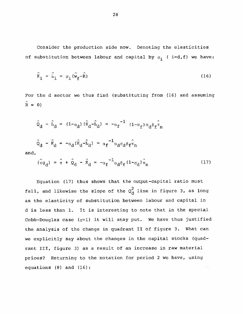
Consider the production side now. Denoting the elasticities

of substitution between labour and capital by c ( id,f) we have:

—La = cY.(WfR) (16)

For the d sector we thus find (substituting from (16) and assuming

= 0)

-Ld

= (l-cd) dd = f (l_cf)adf1rfl

-Kd dd'd = afdadfn

and,

= + d - = fadfdn (17)

Equation (17) thus shows that the output-capital ratio must

fall, and likewise the slope of the line in figure 3, as long

as the elasticity of substitution between labour and capital in

d is less than 1. It is interesting to note that in the special

Cobb-Douglas case (=l) it will stay put. We have thus justified

the analysis of the change in quadrant II of figure 3. What can

we explicitly say about the changes in the capital stocks (quad-

rant III, figure 3) as a result of an increase in raw material

prices? Returning to the notation for period 2 we have, using

equations (8) and (16):

29

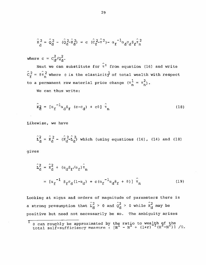
= - (QcKc) = C (C) afaddfTr

22where c = Cd/Qd.

Next we can substitute for ir2 from equation (16) and write

C = Oir where o is the e1asticit of total wealth with respect

to a permanent raw material price change (ir1 = Tr).We can thus write:

= fdf (c_Cd) + cO] r (18)

Likewise, we have

= - (K—L) which (using equations (16), (14) and (18)

gives

L = + dfu/afn

= [af fGd(l_d) + c(fcdBf + 0)] r (19)

Looking at signs and orders of magnitude of parameters there is

a strong presumption that L > 0 and > 0 while may be

positive but need not necessarily be so. The ambiguity arises

1can roughly be approximated by th ratio to wea1h 9f he

total self-sufficiency measure : [H - N + (l+r) (H —N )i /Q.

30

from the fact that 0 is negative for a net importer while in (18)

(c—ad) may or may not be positive.1 If L rises, then by

construction must fall, and since K/L is known to fall in

response to a 1T increase, K must be falling and so do and

We can thus state as an upshot that there is a strong

presumption that employment, output and capital in the f industry

will fall and that employment and output (and maybe capital) in

the d industry will rise.

It is important to stress again that when it comes to drawing

any lessons for reality everything that has been said here about

sectoral changes should be interpreted as deviations from what

long—run trend would otherwise be, and not necessarily as indica-

ting absolute positive or negative levels of investments, etc.

We have assumed zero population growth, no technical progress

and no depreciation of capital. While relaxation of these assump-

tions would not pose particular difficulties, they do simplify the

analysis, but at the same time require that one interpret the

results with suitable modification.

VII. World equilibrium, changes in the rate of interest and the

current account

So far we have conducted the analysis under the assumption

1Numerical example ( with reasonable orders of magnitude):

= 0.6, = 0.4, 0.4, Gd =0.7, c = 0.8, 0= —0.05.

We get (per 1% of ir ): K = 0.02, L = 0.72, Q = 0.44 (percent).

If 0= _O.lO, Kd =-O.O2, Ld = 0.68, 0d = 0.40 (percent). In

both cases, ir = -0.7, Wf = -1.0.

31

that the world rate r* remains constant. This is a very con-

venient device since it appropriately fixes the long—run factor

prices and factor proportions. This particular small economy

assumption need, of course, not hold if one thinks of the impli-

cations of an increase in raw material prices hitting all indus-

trial countries at the same time. In the short and medium run,

as experience has also shown, a shift in the world savings schedule

and an investment short—fail may drive the real rate down, although

it is not clear why this should be sustained for a very long

period. In any case, one may consider the implication of an

exogenous change for a single country within the above model.

Specifically let us consider a drop in r* on top of a permanent

increase in it

A fall inr* causes a rise in w (or rather mitigates the fall

in w). If d is more capital intensive than f, there will be a

further fall in rr2. The same analysis also shows that as

well as fall relatively to their previous long-run solution.

The fall in r raises the present value of wealth (n), and thus

shifts up the curve 2 in figure 3, leading to a relative increase

in consumption, 'rr1 and Q, and a relative fall in Q. Since

the curve stays the same, savings (S1) must fall in the process,

as one would expect.

This will hold as long as the weighted marginal propensity tosave out of wealth of the net exporters of raw materials out-weighs the MPS for the net importers.

32

The outcome in the second period depends on what happens

to consumption demand for non—tradables which in turn is propor-

tional to (l+r) C. The latter may go down since in all prob—

ability Q (and thus C) increases by less than (l+r) falls. So

the question is whether the resulting relative fall in demand

for can outweigh the effect of rising per unit capital

requirements. The term multiplying P in a modified expression for

K (as in (18)) turns out to be

ambiguous in sign.1 Again the presumption is that it

will certainly reduce L. Here the elasticity with respect to R is

—l( dd (l—f)/afJ-3-c

+eLf adyf

which is always positive. If the fall in the rate of interest

reduces L it certainly increases L. With the relative increase

in the capital stock as well as the output of f

in the second period must be higher than otherwise. With the

fall in C = (1+r)C, it turns out that the current account in

the second period (F2) must improve and therefore F1 in the

first period must worsen.2

The final upshot, which makes intuitive sense, is that an

exogenous fall in the interest rate makes for more net foreign

1 For the numerical eample given earlier this equals +0.3, afall in R reduces Kd.

2This would1irnmediately follow if total investment (Ii) rises;savings (S ), as we have seen, certainly falls. The rise ininvestments i proable1but not certain while the fall in thedifference (F = S - I ) is ambiguous.

33

borrowing (or reduction in capital outflow) today at the expense

of the future and this has a counterpart in the structure of

production and consumption. Less production and more consumption

(by imports) of tradables today and more production (less con—

surnption) next period, Correspondingly the relative price fallsless today (a smaller real depreciation) and more tomorrow.

1

This monotonic relationship between r and the current account

can also be used to consider the case in which we do not assume

free capital mobility. Suppose the government sets a target

for the current account which involves a smaller deficit (or

larger surplus) than would be obtained as an endogenouS solution

of the system. 2 This implies government intervention in the

form of fiscal and real exchange rate policy such as implicitly

involves an increase in the domestic real rate of interest. The

implications for the structure of production and consumption in

both periods will be exactly the reverse of that found in the case

previously considered. In other words, there will now be an

increase in savings and in net production of f today at the expense

of less of the same tomorrow, with all the concomitant effects on

patterns of investment and labour use.

The converse may also take place. A government may decide

to run a larger deficit than would otherwise be obtained for

reasons of supporting price stability or full employment. These

1 Again this is not unfamiliar from the trade and developmentliterature (op. cit.).

2 We implicitly assume that only the government now conductsthe foreign borrowing or lending with the budget absorbingthe difference in interest rates.

34

questions will be briefly discussed in the next section.

VIII. Real wage rigidity and other modifications

So far we have assumed wage and price flexibility and

automatic clearing of all markets. Under a raw material price

shock unemployment may arise when real wages are temporarily

downward rigid (see Bruno and Sachs, 1979). For simplicity

consider such rigidity in terms of this periods wage in f1

units (wf). In the extreme case in which wf is held fixed

at its initial level (wf = w in the 'very short-run") a raw

material price increase will now show in a greater reduction

in real wealth since net output of f (Y), for a given wf I fallsby more than it would fall otherwise.2 Wealth (Q) will no

longer depend directly on ri, and the curve in figure 3 (quadrant

I) will now be replaced by a line parallel to the rr axis which

shifts down as Ti increases, to a position like the line passing

through points D0 and D1 in the figure. If ri were also downward

rigid (say the nominal exchange rate were fixed and prices of d

are downward rigid), the economy would momentarily stay at

the point D, where there is excess supply in the commodity

market (the demand for C is less than Q - G1), as well as

unemployment. If commodity prices are free to adjust, Ti1 will

fall and C will rise to the point D0, where the d market clears

More realistically the consumption wage should be expressedin terms of an average of wf and Wf/1T. Real wage rigiditymay thus imply a constraint on the relationship between Wfand ii, rather than on Wf alone.

2 Formally, this can be seen by showing that Yf/tnl -N while

(Yf/7rH —N -(positive term)

Wf

35

clears but labour does not. Full employment could be reached, with

a rigid real wage, at the point D. This corresponds to the case

in which government expenditure is increased to insure full

employment (the line shifts to pass exactly through D),

while taxes are suitably adjusted and domestic consumption

of d falls.

Since consumption along with private wealth must be lower than

in the flexible wage case (which corresponds to the points E1,

E2, etc.), the effect in the second period is to reduce K, L2

and Q (point D in quadrant II) and increase K, L and

relative to what they would otherwise be. This solution

correspondingly implies that there will be a larger surplus

(or smaller deficit) in the current account in the second

period at the expense of the first period in which both domestic

savings and the current account must fall.

The above analysis may look somewhat mechanistic since we

have fixed the real wage independently of the state of the labour

market in which case the size of public expenditure does not seem

to have any quantitative effects in the future. This could

easily be modified by assuming, in Phillips curve fashion, that

Wf changes smoothly as a negative function of the unemployment

rate. In this case this period's changes in G will directly affect

the size of the structural changes in the second period.1

Note that we have assumed that the increase in G1is financedby increased taxes. Had we assumed insted that this isfinanced by a decrease in next period's G (i.e., by debt)the intertempoa1 link would also show directly (by an upwardshift in the line in quadrant II of figure 3).

36

As long as nominal money has not been incorporated in the

model one cannot explicitly analyze inflation and the role of

monetary policy. While this can be remedied formally by intro-

ducing money demand/supply and a nominal interest rate, the

likely role of money can be guessed even without its explicit

introduction. Money may have a real long—term effect in this

model if there is short-term non—neutrality. As in similar

mn1 1 g - ii rm i ii 1 nr jr' (r - - .- xi nii * b -mnrr' .., .1

rigid, in which case real private wealth (as well as Tr and Wf)

may change as a result of monetary policy, thus affecting next

period's factor allocations in a way similar to that analyzed

before.

We conclude our discussion by noting again that, with one

exception, we have so far stuck to the simplification that only

second period's quantities are affected by today's disturbances

while relative prices were assumed to remain invariant. A more

general approach should also allow for induced changes in long—run

relative prices. We briefly mention one example where this may

occur. Suppose we relax the assumption that the f good is a

perfect substitute for the world final good and assume instead

that the individual country faces a downward sloping demand

curve for its product (priced Pf) which is an imperfect substi-

tute for the world final good (whose domestic price is e.p* Pf).

In that case the final goods terms of trade (pf/ep*) become an

37

additional endogenous relative price, which may now move the

final position of the FPF for f (the curve in figure 2),

since the relative price of the raw material will also become1

endogenous [7Th = ep /Pf = (pn*/p*) (ep*/pf)]• What this

implies is that present period's stabilization policies may

affect next period's 2 and w even though r* is given. Once

we introduce these and additional complications, however, there

remains less advantage in considering an analytical model over

simulations with a more realistically complex empirical framework.

After all we set out with the objective of showing that consider-

able insight into some of the issues can be gained by looking

at a stripped-down version of such a model.

1 Such argument, for a medium term context, explains why in faceof the same external price shock (in terms of p*/p*) a countrylike Germany suffered a smaller internal increase in in the1970s, compared to Japan or the U.K. (The implications for thedifferential productivity performance in manufacturing arediscussed in Bruno, 1981.)

38

References

Bardhan, P., "Optimal Foreign Borrowing," in K. Shell (ed.),Essays in the Theory of Optimal Growth, The MIT Press,1966.

Berndt, E.R., and D.O. Wood, "Engineering and EconometricInterpretation of Energy-Capital Complementarity," AmericanEconomic Review, June, 1979.

Bruno, M., "Optimal Patterns of Trade and Development," TheReview of Economics and Statistics, November 1967.

____ "Raw Materials, Profits and the Productivity Slowdown,"Discussion Paper No. 812, Falk Institute, Jerusalem, April1981. (Also appeared as NBER Working Paper No. 660).

Bruno, M., and J. Sachs, "Supply versus Demand Approaches tothe Problem of Staqflation," NBER Working Paper No. 382,August 1979- (Appeared in Macroeconomic Policies for Growth andStability, Institut fur Weltwirtschaft, Kiel, 1981.)

"Input Prices Shocks and the Slowdown in Economic Growth:Estimates for U.K. Manufacturing," presented at the Confer-ence on Unemployment, Newnham College, Cambridge, July 198L

Corden, W.M., and J.P. Neary, "Booming Sector and de—Industrial—ization in a Small Open Economy," mimeo, 1980.

Mayer, W., "Short-Run and Long-Run Equilibrium for a Small OpenEconomy," Journal of Political Economy, September/October1974.

Neary, J.P., and D.D. Purvis, "Sectoral Shocks in a DependentEconomy: Short-Run Accomodation and Long-Run Adjustment,"mirneo, 1981.

Razin, A., "Capital Movements, Intersectoral Resource Shifts,and the Trade Balance," Seminar Paper No. 159, Institutefor International Economic Studies, University of Stockholm,October 1980.

Sachs, J., "Energy and Growth under Flexible Exchange Rates,"NBER Working Paper No. 582, November 1980; also forthcomingin Bhandari and Putnam (eds.), The International Transmission

39

of Economic Disturbances under Flexible Exchange Rates,forthcoming, MIT Press, 1982.

____ "Aspects of the Current Account Behavior of OECD Economies,"presented at the Vth International Conference of the Universityof Paris—Dauphine on Money and International Monetary Problems,June 1981.

Svensson, L.E.O., "Oil Prices and a Small Oil—Importing Economy'sWelfare and Trade Balance: An Intertemporal Approach," Insti-tute for International Economic Studies, University ofStockholm, October 1981.

van Wijnbergen, S., "Optimal Investment and Exchange Rate Manage-ment in Oil Exporting Countries: A Normative Analysis of theDutch Disease," mimeo, Development Research Center, WorldBank, Washington, 1981.