TRANSPORTATION RESEARCH RECORD 1286 123

MICH-PA VE: A Nonlinear Finite Element Program for Analysis of Flexible Pavements

RONALD s. HARICHANDRAN, MING-SHAN YEH, AND GILBERT Y. BALADI

A nonlinear mechanistic finite element program called MICH­p A VE has been developed for use on personal computers to aid in the analysis and design of flexible pavements. The program has three major features. First, it utilizes a newly developed flex­ible boundary concept for pavement analysis. Second, it uses performance models for the prediction of fatigue life and rut depth, utilizing results of the mechanistic analysis (stresses, strains, and other pavement variables). Third, it is "user-friendly." The program was developed for the Michigan Department of Trans­portation and is in the public domain. The methodology used, and the features of the program, are described.

More and more in recent years pavement design is being based on mechanistic analysis. The migration from empirical meth­ods to mechanistic analysis has been facilitated by the avail­ability of relatively inexpensive microcomputers that can be used in daily practice. Early computer programs for mechan­istic analysis (such as CHEV5L, BISAR, ELSYM5, etc.) modeled pavements as being composed of linear elastic layers and computed deflections, stresses, and strains within a pave­ment arising from a wheel load. In these programs each pave­ment layer is assumed to extend infinitely in the horizontal directions, allowing the three-dimensional problem to be reduced to an axisymmetric two-dimensional problem. Because of the linear elastic assumption, multiple wheel loads can be analyzed by superposing the results from single wheel loads.

The main drawbacks of these linear elastic layer programs are that

• They cannot model the nonlinear resilient behavior of granular and cohesive soils;

•They normally assume weightless pavement material; • They may yield tensile stresses in granular material, which

cannot physically occur; and • They do not account for "locked-in" stresses from com­

paction during construction.

To overcome these shortcomings, nonlinear analysis programs based on the finite element method have been developed (e.g., ILLI-PAVE). However, because of the large memory and computational effort requirements, these programs pri­marily have been implemented on mainframe computers. Fur-

R. S. Harichandran and G. Y. Baladi, Department of Civil and Envi­ronmental Engineering, Michigan State University, East Lansing, Mich. 48824. M-S. Yeh, Engineering Office of Taipei Railway Under­ground Project, 3 Pei-Ping West Road, 3rd Floor, Taipei, Taiwan 100, Republic of China.

ther, the interaction of the user and these programs, in terms of data input and interpretation of the output, is not "friendly," making their use in daily practice undesirable.

For most state highway agencies, a "user-friendly" flexible pavement program that can be used for the design or reha­bilitation of flexible pavements in daily practice is desired. This program should consider all the major factors affecting the design or rehabilitation of pavements. To achieve this, a research study was sponsored by Michigan Department of Transportation (MDOT). The main goal of this research was to review existing analysis and design methods and then to develop a user-friendly nonlinear finite element program that can be used on personal computers in daily practice. Since current personal computers have limited memory capacities, the traditional finite element method, which requires a large amount of memory, cannot be suitably implemented on them unless accuracy is sacrificed. To overcome this shortcoming, Harichandran and Yeh (1) proposed a new technique of plac­ing a relatively shallow finite element mesh on a flexible boundary. This technique substantially reduces the memory and computational requirements of the nonlinear finite ele­ment method without sacrificing accuracy. In this research, this technique is implemented with user-friendly input and output features, to develop a nonlinear finite element pro­gram for the analysis and design of flexible pavements. The program has been named MICH-PAVE.

MATERIAL NONLINEARITY

There are many nonlinear material models that may be used in mechanistic analysis. Four suitable models-the hyper­bolic, the resilient modulus, the shear and volumetric stress­strain (also called the contour model), and the third-order hyperelastic models-were reviewed (2-7). Of these, the resilient modulus model was chosen as the most suitable at the present time. This choice is based on the applicability of the model to repeated loading patterns experienced by pave­ments, and on the relative ease of determining the model parameters by state highway agencies. The resilient modulus model characterizes the resilient stress-strain properties of soils through a stress-dependent modulus and a constant Pois­son ratio.

For granular soils, the resilient modulus is characterized as

(1)

124

Log Bulk Stress (Log 9)

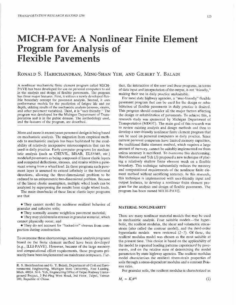
FIGURE 1 Resilient modulus model for granular material.

where M, = resilient modulus (psi), 0 = u, + rr2 + rr3 = bulk stress (psi), and Ki and K2 are material constants. This relationship is illustrated in Figure 1.

For cohesive soils, the resilient modulus is expressed through the bilinear relationship

for K i > (rr1

for K i :5 (rr1

(2)

where (rri - rr3) = deviator stress (psi), and K,, K 2 , K3 , and K 4 are material constants. This relationship is illustrated in Figure 2.

If the finite element method is used with only the resilient modulus model, it will converge extremely slowly . Therefore, Raad and Figueroa (8) applied the resilient modulus model with the Mohr-Coulomb failure criterion. The Mohr-Coulomb failure criterion is used to modify the principal stresses of each element in the granular layers and roadbed soil after each iteration so as not to exceed the Mohr-Coulomb failure envelope. Thompson (9) used this algorithm in the ILLI­PA VE program. A similar algorithm was developed for MICH­PAVE.

FEATURES OF THE MICH-PAVE PROGRAM

The MICH-PA VE program is capable (depending on the user's choice) of performing either linear or nonlinear finite element analysis of flexible pavements. It assumes axisymmetric load­ing conditions arising from a single circular wheel load on pavement layers of infinite horizontal extent. The various features of the program are described in this section . Tech­nical details and results from various sensitivity analyses can be found elsewhere (10,11).

Mesh Generation and Flexible Boundary

The finite element method needs to satisfy some basic require­ments for the mesh, such as the location of the side and bottom boundaries, the size and shape of the elements, and the dis­tribution of the elements in the various regions . To establish criteria for locating the boundaries in a finite element mesh,

TRANSPORTATION RESEARCH RECORD 1286

Mr

\ "I I•

K1 •I Deviator Stress (a - a )

1 3

FIGURE 2 Resilient modulus model for cohesive material.

Duncan et al. (12) showed comparisons between displace­ments and stresses computed using the finite element method and those computed using elastic half-space and layered sys­tem analysis.

For an elastic half-space subjected to a uniform circular load, displacements and stresses computed by the finite ele­ment method compare well with those determined from the Boussinesq solution, when

• the bottom boundary in the finite element mesh is fixed at a depth of about 18 radii of the loaded area ; and

• the vertical side boundary is located at a distance of about 12 radii from the center and constrained from moving radially.

For a three-layered system, a reasonable comparison between the two procedures can be obtained if the bottom boundary in the finite element mesh is moved to a depth of about 50 radii, while maintaining the side boundary at 12 radii.

Previous experience has shown thal stresses based on quad­rilateral elements will be accurate provided that the length­to-width ratio for the elements does not exceed five to one. Furthermore, smaller elements should be used close to the loaded area, and progressively larger elements may be used in the regions away from the loaded region.

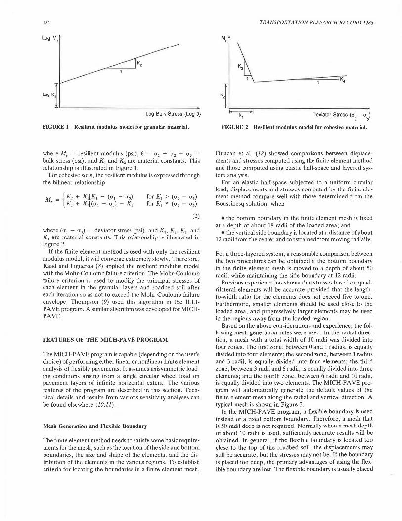
Based on the above considerations and experience, the fol­lowing mesh generation rules were used. In the radial direc­liun, a mesh wilh a Lota! width of 10 radii was divided into four zones. The first zone, between 0 and 1 radius , is equally divided into four elements; the second zone, between 1 radius and 3 radii, is equally divided into four elements; the third zone, between 3 radii and 6 radii, is equally divided into three elements; and the fourth zone, between 6 radii and 10 radii, is equally divided into two elements. The MICH-PAVE pro­gram will automatically generate the default values of the finite element mesh along the radial and vertical direction. A typical mesh is shown in Figure 3.

In the MICH-PA VE program, a flexible boundary is used instead of a fixed bottom boundary. Therefore, a mesh that is 50 radii deep is not required. Normally when a mesh depth of about 10 radii is used, sufficiently accurate results will be obtained. In general, if the flexible boundary is located too close to the top of the roadbed soil, the displacements may still be accurate, but the stresses may not be. If the boundary is placed too deep, the primary advantages of using the flex­ible boundary are lost . The flexible boundary is usually placed

Harichandran et al.

Asphalt

Granular

Roadbed Soil

l 11

0 a 3a 6a

Depth

0.0"

10.0"

30.0"

10a50.0"

125

Radial Distance in Radii (Radius of loaded area, a= 5.35 in)

FIGURE 3 Typical finite element mesh.

at about 12 in. below the upper surface of the roadbed soil, or at a depth of 50 in., whichever is greater. In the MICH­PA VE program, the depth at which the flexible boundary is placed is specified by the user, by inputting the depth of the roadbed soil to which stress and strain calculations are required. If the boundary is placed at a depth of Jess than about 50 in., then the stresses still will be accurate, but the vertical deflec­tions may be overestimated.

Modulus of Half-Space Below Flexible Boundary

The half-space below the flexible boundary is assumed to be homogeneous and linear elastic. The boundary is therefore always placed within the last layer (roadbed soil). Although the modulus of the roadbed soil below the boundary may in reality be stress dependent and vary from one location to another, in most pavement. sections the stresses from wheel loads are substantially diminished at the level of the roadbed soil. Thus, the use of a constant modulus below the boundary has a negligible effect on the stresses and displacements above the boundary. In MICH-PAVE, the modulus used for the half-space below the boundary is the average moduli of the finite elements immediately above the boundary. To avoid undesirable "edge effects," the elements closest to the right vertical boundary are not used in computing this average.

Gravity and Lateral Stresses

The MICH-PA VE program includes the effect of gravity and lateral stresses arising from the weight of the materials. At any location within the pavement, the vertical gravity stress (cr8) is computed as the accumulation of the layer thicknesses multiplied by the appropriate unit weights .

The lateral stress (crh) is calculated from the coefficient of earth pressure at rest (K0 ) and vertical gravity stress, as

(3)

where

K 0 = 1 - sin <!> for cohesionless soil and gravel; K 0 = 1 - 0.95 sin<!> for cohesive soil; and

<!> = angle of internal friction.

To approximately account for "locked-in" stresses caused by compaction, the user can input a value for K 0 higher than the coefficient of earth pressure at rest.

Iterative Solution and Convergence Criterion

MICH-PA VE performs nonlinear analysis by the following steps:

1. Initially, the wheel load at the surface is assumed to spread over a 2:1 region (i.e., the radius of the loaded area is assumed to increase by 1 in . for every 2 in. of depth). The stresses arising from this assumed distribution of the wheel load are combined with gravity stresses , to compute the initial resilient moduli for each of the finite elements in granular and cohesive materials.

2. A linear analysis is performed, and a more accurate stress distribution is computed.

3. For those elements that exceed the Mohr-Coulomb fail­ure criterion, the computed stresses are adjusted according to the procedure outlined by Raad and Figueroa (8).

4. A new value of the resilient modulus is computed for each element based on the latest stresses.

5. Convergence in the resilient moduli is checked by com­puting the relative error, e = l (M,,, - M,,,_ 1)2/l M;.,_,, where M,,, are the current resilient moduli, M,,,_ 1 are the previous resilient moduli, and the summations are taken over all nonlinear elements.

6. Steps 2 through 5 are repeated until the relative error e is less than 0.001.

126

7. Displacements, strains, and stresses are then computed at all specified locations, and the fatigue life and rut depth of the pavement are estimated.

Interpolation and Extrapolation of Stresses and Strains at Layer Boundaries

For a pavement section in which various layers are fully bonded (i.e . , when no slip occurs at layer boundaries), quantities such as the vertical and shear stresses and the radial and tangential strains should be continuous across layer interfaces. However, because of the low-order interpolation functions chosen in the finite element approach, these quantities are not continuous across element boundaries. Thus, if these quantities are esti­mated by finite element approach at two adjacent points across an interface, the results will show an apparent discontinuity that is an artifact arising from the error in the finite element method. This result is undesirable and can be overcome by using linear interpolation to estimate these quantities at an interface from those at the middle of the adjacent elements. For example, if a 1 is the stress at the center of an element immediately above the interface and a 2 is the stress at the center of an element immediately below the interface, then the stress at the interface obtained by linear interpolation is

(4)

where z1 and z2 are the depths of the points at which a 1 and a 2 are evaluated, and z is the depth of the interface.

Smee the finite element approach gives accurate estimates of stresses and strains at the center of elements, but can yield significant error at element edges, even those stresses and strains at the interfaces that are discontinuous across the inter­face can be in significant error. For quantities such as the radial and tangential stresses that are discontinuous across an interface, it is possible to estimate their values at one side of the interface by linear extrapolation of the values at the center of two elements on that side of the interface. For example, if a 1 and a 2 are stresses at the center of two consecutive elements below (or above) an interface, then the linearly extrapolated stress at the lower (or upper) side of the interface is also given by Equation 4, where z1 and z2 are the depths of the points at which a 1 and a 2 are estimated, and z is the depth of the interface.

TRANSPORTATION RESEARCH RECORD 1286

Finally, based on prior knowledge of the solution (vertical and shear stresses must be zero at the surface, except for the vertical stress below the wheel load, which must be identical to the tire pressure), the surface stresses are arbitrarily set to their proper values in MICH-PA VE.

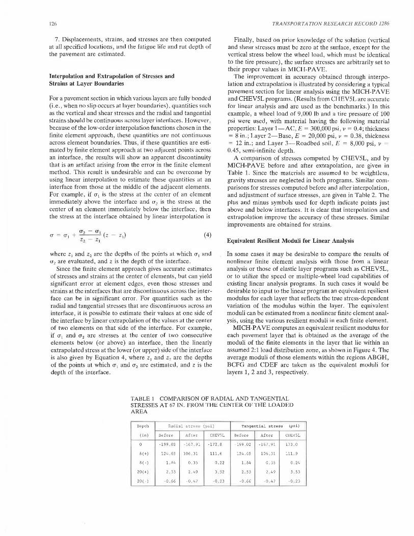
The improvement in accuracy obtained through interpo­lation and extrapolation is illustrated by considering a typical pavement section for linear analysis using the MICH-PAVE and CHEVSL programs. (Results from CHEVSL are accurate for linear analysis and are used as the benchmarks.) In this example, a wheel load of 9,000 lb and a tire pressure of 100 psi were used, with material having the following material properties: Layer 1-AC, E = 300,000 psi, v = 0.4; thickness = 8 in.; Layer 2-Base, E = 20,000 psi, v = 0.38, thickness = 12 in. ; and Layer 3-Roadbed soil, E = 8,000 psi, v =

0.45, semi-infinite depth. A comparison of stresses computed by CHEV5L, and by

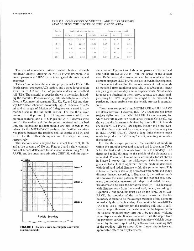
MICH-PAVE before and after extrapolation, are given in Table 1. Since the materials are assumed to be weightless, gravity stresses are neglected in both programs. Similar com­parisons for stresses computed before and after interpolation, and adjustment of surface stresses, are given in Table 2. The plus and minus symbols used for depth indicate points just above and below interfaces. It is clear that interpolation and extrapolation improve the accuracy of these stresses. Similar improvements are obtained for strains.

Equivalent Resilient Moduli for Linear Analysis

In some cases it may be desirable to compare the results of nonlinear finite element analysis with those from a linear analysis or those of elastic layer programs such as CHEV5L, or to utilize the speed or multiple-wheel load capabilities of existing linear analysis programs. In such cases it would be desirable to input to the linear program an equivalent resilient modulus for each layer that reflects the true stress-dependent variation of the modulus within the layer. The equivalent moduli can be estimated from a nonlinear finite element anal­ysis, using the various resilient moduli in each finite element.

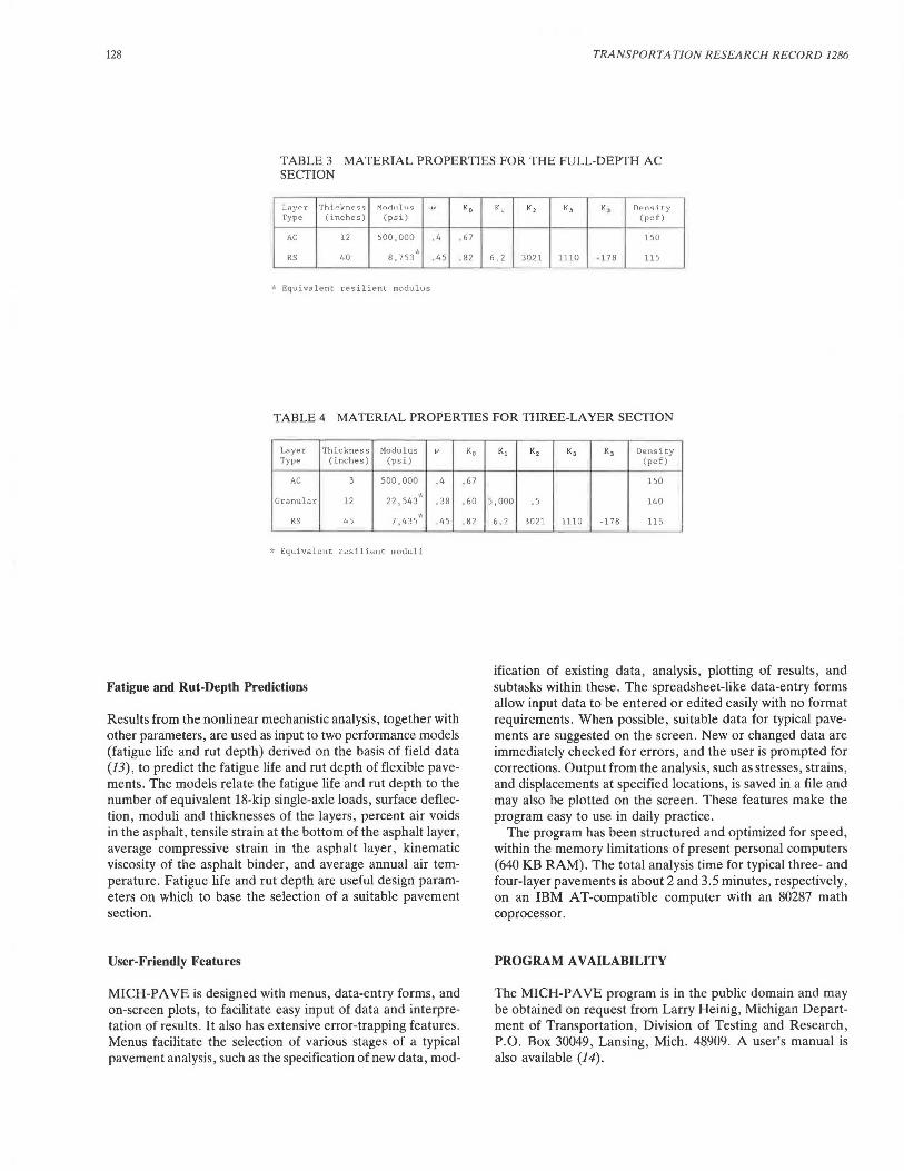
MICH-PA VE computes an equivalent resilient modulus for each pavement layer that is obtained as the average of the moduli of the finite elements in the layer that lie within an assumed 2:1 load distribution zone, as shown in Figure 4. The average moduli of those elements within the regions ABGH, BCFG and CDEF are taken as the equivalent moduli for layers 1, 2 and 3, respectively.

TABLE 1 COMPARISON OF RADIAL AND TANGENTIAL STRESSES AT 67 IN. FROM THE CENTER OF THE LOADED AREA

Depth Radial stress (psi) Tangential stress (psi)

(in) Before After CHEV5L Before After CHEV5L

0 -199 02 -167 . 91 -172 . 8 -199.02 ·16 7. 91 -173 . 0

8(+) 124 . 65 106. 31 111 . 6 124' 65 106.31 111. 9

8 ( - ) 1 84 0 , 35 0 . 22 1.84 0 . 35 0. 24

20(+) 2 . 53 2 . 49 3 . 52 2 . 53 2 . 49 3 . 53

20(.) -0 . 66 -0 . 47 -0 . 23 -0. 66 -0 47 -0 . 23

Harichandran et al. 127

TABLE 2 COMPARISON OF VERTICAL AND SHEAR STRESSES AT 67 IN. FROM THE CENTER OF THE LOADED AREA

Depth Vertical stress (psi) Shear stress (psi)

(in) Before After

0 14 3 . 5 7 100 , 0

8(+) 0 0 12 70

8 (.) 9 15 12 70

20(+) 3 . 03 3 . 10

20(.) 1.61 3 . 10

The use of equivalent resilient moduli obtained through nonlinear analysis utilizing the MICH-PAVE program, in a linear program (CHEV5L), is investigated through typical examples.

Tables 3 and 4 show the material properties of a 12-in. full­depth asphalt concrete (AC) section , and a three-layer section with 3 in . of AC and 12 in. of granular material on roadbed soil (RS). The material properties shown in the tables, includ­ing the modulus , Poisson ratio (v), lateral earth pressure coef­ficient (K0 ), material constants (K1, K2 , K3 , and K4) and den­sity have been obtained previously (5). A cohesion of 6.45 psi and an angle of friction of 0 degrees were used for the roadbed soil in the full-depth section. For the three-layer section, c = 0 psi and cl> = 45 degrees were used for the granular material and c = 6.45 psi and cl> = 0 degrees were used for the roadbed soil. For the granular material and roadbed soil, the equivalent resilient moduli are also shown in the tables. In the MICH-PAVE analysis, the flexible boundary was placed beneath the roadbed soil, at depths of 52 in . and 60 in. for the full-depth asphalt and three-layer sections, respectively.

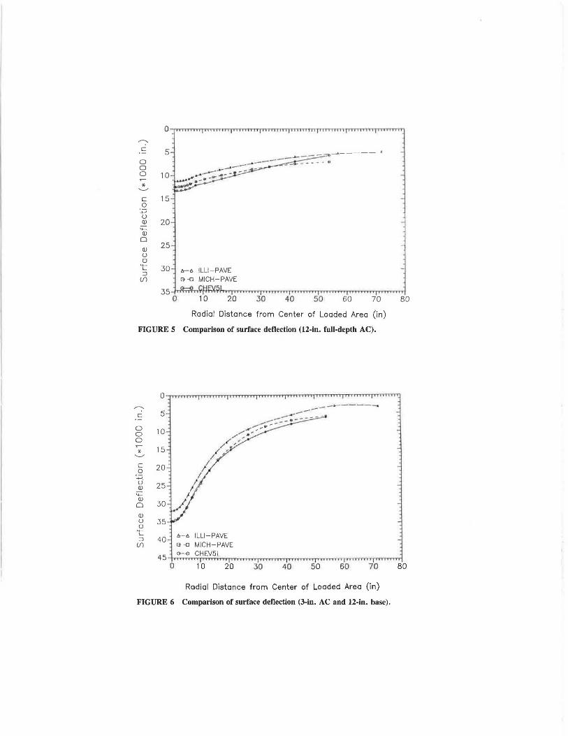
The sections were analyzed for a wheel load of 9,000 lb and a tire pressure of 100 psi. Figures 5 and 6 show compar­isons of surface deflections for nonlinear analysis using MICH­p A VE, and the linear analysis using CHEV5L with the equiv-

Layer1

Layer 2

' I i : . I I ! I , 1 , .j ... ... +- .... j .... ........ 1 ...... : ......... - ..................... _ ... ..

! i ·1 i 2 ! ! ! i 1 .i .. . .... j .... --~-· .... - .. 1 ....... i.-- . . ........ _ .. _ ........ ...... _,

I I I ! I D I : I I !

Layer 3

Flexible Boundary

FIGURE 4 Elements used to compute equivalent resilient moduli.

GHEV5L Before After GHEV5L

99 , 7

12 . 25

12 . 25

3.36

3 , 36

2. 62 0 , 0 0.0

3 . 29 2 69 0 55

0. 65 2 . 69 0.55

0 . 12 0 . 11 0 , 07

0 , 07 0 , 11 0 07

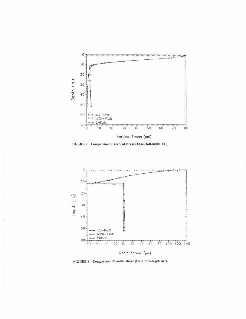
alent moduli. Figures 7 and 8 show comparisons of the vertical and radial stresses at 0.5 in. from the center of the loaded area. Deflections and stresses computed by the nonlinear finite element program ILLI-P A VE are also shown in these figures.

The results indicate that the use of equivalent resilient mod­uli obtained from nonlinear analysis, in a subsequent linear analysis, gives reasonably similar displacements. Notable dif­ferences are obtained in the stresses, because the linear anal­ysis using CHEV5L neglects the weight of the material. In particular , linear analysis can give tensile stresses in granular soils.

The stresses computed using MICH-PAVE and ILLI-PAVE are almost identical. However, ILLI-PAVE tends to give lower surface deflections than MICH-PAVE. Linear analysis, for which accurate results can be obtained through CHEV5L, has shown that displacements obtained by using a flexible bound­ary (as in MICH-PAVE) are slightly greater and more accu­rate than those obtained by using a deep fixed boundary (as in ILLI-PA VE) (10,11) . Using a deep finite element mesh tends to produce a "stiffening" effect , resulting in smaller displacements.

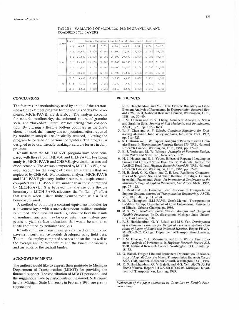
For the three-layer pavement, the variation of modulus within the granular layer and roadbed soil is shown in Table 5 for the first eight elements from the left boundary. The depth and radial distance to the middle of the elements are tabulated. The finite element mesh was similar to that shown in Figure 3, except that the thicknesses of the layers are as given in Table 4. It is apparent that the modulus decreases with depth and radial distance within the granular layer. This is because the bulk stress (0) decreases with depth and radial distance; hence, according to Equation 1, the resilient mod­ulus follows the same pattern. Within the roadbed soil , how­ever, the modulus increases with depth and radial distance. This increase is because the deviatoric stress ( u 1 - u 3) decreases with distance away from the wheel load; hence, according to Equation 2, the modulus must also do the same. In MICH­p A VE, the modulus of the half-space below the flexible boundary is taken to be the average modulus of the elements immediately above the boundary. Care must be taken in MICH­p A VE to use a thickness for the roadbed soil that is suffi­ciently deep; otherwise the modulus of the half-space below the flexible boundary may turn out to be too small, yielding large displacements. It is recommended that the depth from the pavement surface to the flexible boundary (which is deter­mined by the user inputs of layer thicknesses including that of the roadbed soil) be about 50 in. Larger depths have no appreciable effect on displacements.

128 TRANSPORTATION RESEARCH RECORD 1286

TABLE 3 MATERIAL PROPERTIES FOR THE FULL-DEPTH AC SECTION

LAyer Thir:-l<'nr:><;;c; M0d11l115 " Ko Kl K, K, K, npn.:; i ry Type (inches) (psi) (pcf)

AC 12 500,000 ' 4 6 7 150

* RS 40 8,753 .45 . 82 6. 2 3021 1110 · 178 115

* Equivalent resilient modulus

TABLE 4 MATERIAL PROPERTIES FOR THREE-LA YER SECTION

Layer Thickness Modulus v Type (inches) (psi)

AC 3 500,000 . 4

* Granular 12 22' 543 . 38

* RS 45 7 ,435 45

* Equivalent resilient moduli

Fatigue and Rut-Depth Predictions

Results from the nonlinear mechanistic analysis, together with other parameters, are used as input to two performance models (fatigue life and rut depth) derived on the basis of field data (13), to predict the fatigue life and rut depth of flexible pave­ments. The models relate the fatigue life and rut depth to the number of equivalent 18-kip single-axle loads, surface deflec­tion, moduli and thicknesses of the layers, percent air voids in the asphalt, tensile strain at the bottom of the asphalt layer, average compressive strain in the asphalt layer, kinematic viscosity of the asphalt binder, and average annual air tem­perature. Fatigue life and rut depth are useful design param­eters on which to base the selection of a suitable pavement section.

User-Friendly Features

MICH-PA VE is designed with menus, data-entry forms, and on-screen plots , to facilitate easy input of data and interpre­tation of results. It also has extensive error-trapping features. Menus facilitate the selection of various stages of a typical pavement analysis, such as the specification of new data, mod-

Ko

.6 7

. 60

82

K, K, Ka Ka Density (pcf)

150

5' 000 . 5 140

6 ' 2 3021 1110 · 178 115

ification of existing data, analysis, plotting of results, and subtasks within these. The spreadsheet-like data-entry forms allow input data to be entered or edited easily with no format requirements. When possible, suitable data for typical pave­ments are suggested on the screen. New or changed data are immediately checked for errors, and the user is prompted for corrections. Output from the analysis, such as stresses, strains, and displacements at specified locations, is saved in a file and may also be plotted on the screen. These features make the program easy to use in daily practice.

The program has been structured and optimized for speed, within the memory limitations of present personal computers (640 KB RAM). The total analysis time for typical three- and four-layer pavements is about 2 and 3.5 minutes, respectively, on an IBM AT-compatible computer with an 80287 math coprocessor.

PROGRAM AVAILABILITY

The MICH-PA VE program is in the public domain and may be obtained on request from Larry Heinig, Michigan Depart­ment of Transportation, Division of Testing and Research, P.O. Box 30049, Lansing, Mich. 48909. A user's manual is also available (14).

,.-..,

c 5 ___,.._ ___ _ 0 0 0 10

* .._,

c 15 0

'..::; u Q) 20

'+--Q)

0

Q) 25

u 0

'+-- 30 L :J t.--6 ILLl-PAVE

(/) 13- -a MICH-PAVE

{fj:IOO,l,,, 111' """1 """"'I'"""" I" 1111

"' I"''''"' I''" ""' 10 20 30 40 50 60 70 80

Radial Distance from Center of Loaded Area (in)

FIGURE S Comparison of surface deflection (12-in. full-depth AC).

c

0 0 0

* c 0 t;. Q)

'+-­Q)

0 Q) u 0

'+­I.. :J

(/)

0 -rr.-1111111111111111111111111• 11111111111111 111111 11 1 1111 'I'''

5

10

15

20

25

35

40 t.--6 ILLl-PAVE ct -a MICH-PAVE

45-t-rTG--0..,.,.,.,...-rp-.-nrn-ITT,..,.,.'rnTnrrt",.,..,....,.,.,.,.,..,..,.,..,..,.,...,..,..,.,.,,...,....,.,.TTTTnTnOTTTTTTJ"ITnrTj

0 10 20 30 40 50 60 70

Radial Distance from Center of Loaded Area (in)

FIGURE 6 Comparison of surface deflection (3-in. AC and 12-in. base).

80

,......__

c .._,, _c ..., 0.. Q)

0

0 ]'""""I""'''" I'""'" ' I'""'" ' I"'" ""I' ""rrrfl'TTTTI . l ___...--

10 -------------~~-~-----

20 t I

\ •

30

40

50

60 l>--t. ILLl-PAVE &-8 MICH-PAVE

70.J.n,.,.,.,.-rrnrri...-r.;;...,.,~~~~~~~~~~~~~~~~~.....i

0 20 30 40 50 60 70 80

Vertical Stress (psi)

FIGURE 7 Comparison of vertical stress (12-in. full-depth AC).

,......__

c .._,, _c +-' 0.. Q)

0

0

10

20

30

40

50 ·--· &-D

ILLl-PAVE MICH-PAVE

60 G---0 CHEV5L

-80 -60 -40 -20

l

I 0 20 40 60 80 1 00 1 20 1 40

Radial Stress (psi)

FIGURE 8 Comparison of radial stress (12-in. full-depth AC).

131 Harichandran et al.

TABLE 5 VARIATION OF MODULUS (PSI) IN GRANULAR AND ROADBED SOIL LAYERS

Depth Radial Distance from Center of Wheel Load (inches) Layer

(in.) 0 . 67 2.01 3.35

4.2 36, BOO 35 '400 32 '200

6 .6 31, 600 30' 500 28' 600

Gran , 9 . 0 25 '800 25 '200 24,200

11.4 21,400 21,100 20' 600

13 8 18' 200 18,100 17' 800

22 5 5 ,640 5,660 5,690

RS 37 . 5 7,340 7,350 7' 360

52 . 5 B, 250 8 '250 8,260

CONCLUSIONS

The features and methodology used by a state-of-the-art non­linear finite element program for the analysis of flexible pave­ments , MICH-PA VE , are described. The analysis accounts for material nonlinearity, the unbound nature of granular soils, and " locked-in" lateral stresses arising from compac­tion . By utilizing a flexible bottom boundary in the finite element model, the memory and computational effort required by nonlinear analysis are drastically reduced , allowing the program to be used on personal computers . The program is designed to be user friendly, making it suitable for use in daily practice.

Results from the MICH-PA VE program have been com­pared with those from CHEV5L and ILLI-PA VE. For linear analysis, MICH-PA VE and CHEV5L give similar strains and displacements. The stresses computed by MICH-PA VE, how­ever, account for the weight of pavement materials that are neglected by CHEV5L. For nonlinear analysis, MICH-PAVE and ILLI-PAVE give very similar stresses, but displacements computed by ILLI-PAVE are smaller than those computed by MICH-PAVE. It is believed that the use of a flexible boundary in MICH-PA VE alleviates the "stiffening" effect that results when a deep finite element mesh with a fixed boundary is used .

A method of obtaining a constant equivalent modulus for a pavement layer with a stress-dependent resilient modulus is outlined. The equivalent modulus, estimated from the results of nonlinear analysis, may be used with linear analysis pro­grams to yield surface deflections that would be similar to those computed by nonlinear analysis.

Results of the mechanistic analysis are used as input to two pavement performance models developed using field data . The models employ computed stresses and strains , as well as the average annual temperature and the kinematic viscosity and air voids of the asphalt binder.

ACKNOWLEDGMENTS

T he authors would like to expres their gratitude to Michigan D epartment of Tran ·portation (MOOT) for providfog the financial support. The conlributio n of MOOT personnel and the suggestions made by participants of the 4-week NH.I course held at Michigan State University in February 1989, are greatly apprecia ted.

4.68 6. 69 9 . 37 12 . 04 14 , 72

27' 800 22, 100 15,300 12,000 10' 300

26' 100 20,400 16' 000 12,700 10' 900

22 '700 20,300 15,500 13' 200 11, 500

19 ,700 18,500 16,100 13 '000 11, 900

17. 400 16,800 15.500 14,000 12,100

5 ,750 5,860 6,040 6,290 6,580

7,380 7 '430 7,520 7,630 7,750

B, 260 B, 270 8,300 B,340 8,380

REFERENCES

1. R. S. Harichandran and M- . Yeh. Flexible Boundary ia Finite Elcrnout Annlysis of Pwcrnent . In Tra11 portatio11 Nesearch Rec· ord 1207, TRB , National Re enrch Council , Washington. 0 . . , 1988, pp. 50- 60.

2. J . M. Duncan and C. Y. Chang. Nonlinear Analy i of trc s and train in Soils. Joumal of Soil Meclumics 011d Fo1111da1io11s , ASCE l970, pp. L629- l653 .

3. W. F. hen and A. F. Salecb . 011sti1ute £q11"'io11s for E11si· 11eeri11g Mmerials. John Wiley, nd S n . Inc., New York , 1982, pp. 516- 525.

4. S. F. Brown and J . W. Pappin. Analy is of Pav mcnt with Gran· ular Bases. Jn TrallSporwtio11 Research Record 810. TRB , at ional Research Council , Washington, D.C., 1981. pp. 17- 23.

5. E. J. Yoder and M. W. Witczak. Pri11ciples of Pa11eme11t Design, John Wiley and ns, Inc. , New York, 1975.

6. H . J. Haynes and E. J. Yoder. Effects of Repemed Loading n Gravel and Crushed tone Base our.;e Mat ria l U cd in the AASHO Road Test. Highway Re. earc/r Recor<l 39, T R13 , National Re.search unci l, Wn hington, D. . '1963, pp. 82-' 6.

7. H . B. Seed, . K. han, and . E. Lee. Resilience Char11cter­islic of Subgrnde Soils and Their Relation to Fatigue Failures in Asphalt Pavement . Proc. , ./st lnum1a1io11a/ 011fere11ce 011 the Stmc111ra/ Design of M plwl1 Pave111e11is, Ann Arbor, Mich., 1962, pp. 77- 111.

8. L. Raad and J . L. Figueroa . Load Response of Tran ponntion Supp rt Sy tern . Journal of Tm11Sportatio11 E11gineeri11g, AS E, Vol. 106, 19 0, pp. 1.l'l - 128.

9. M. R. Thompson. JLLl-PAVE, User's Manual. Tran portation Facilities Group , Department or Civil Engineering. Universi ty or Illinois, Urbana· hampaign, 19 6.

10. M. S. Yeh. Nonlinear Finile Element Analysis a11d De ign of Flexible Pavemellfs. Ph.D. dissertation. Michigan tale Unive r­sity, East Lansing, 1989.

11 . R. S. Harichandran, G. Y. Baladi, and M- . Yeh. Develop1111111t of a Compuler Program for De.sign of Pa veme111 System on· sistillg of Layers of Bound and U11bow1d Materials. Report FHWA· MI-RD-89-02. Michigan epanment ofTransportntion Lansing 1989.

12. J . M. Duncan, C. L. Monismitb . and E. L. Wilson. Finite Ele­ment Analysi of Pavements. ln Highway Research Record 228, TRB, Naliooal Research o"Uncil , Wa hington, D . . , 1968, pp. 18- 33.

13. G. 'Baladi . Fa1.igue Life and l'ermanent Deformation haracter· istics of Asphalt oncretc Mixe . Tra11spor1111io11 Research Record 1227 TRB, ationalRescarch ouncil Washingt n D .. 1989.

14. R. S. 1-larichandran, G. Y. Baladi, and M-S. Yeh. MICH-PAVE User's Ma1111al. Report FHWA-Ml ·RD-89-03. Michiga n Depart­ment of Tran portation, Lansing, 1989.

Publication of this paper sponsored by Committee on Flexible Pave­ment Design.