7-7-11

MGMG 522 : Session #7MGMG 522 : Session #7Serial CorrelationSerial Correlation

(Ch. 9)(Ch. 9)

7-7-22

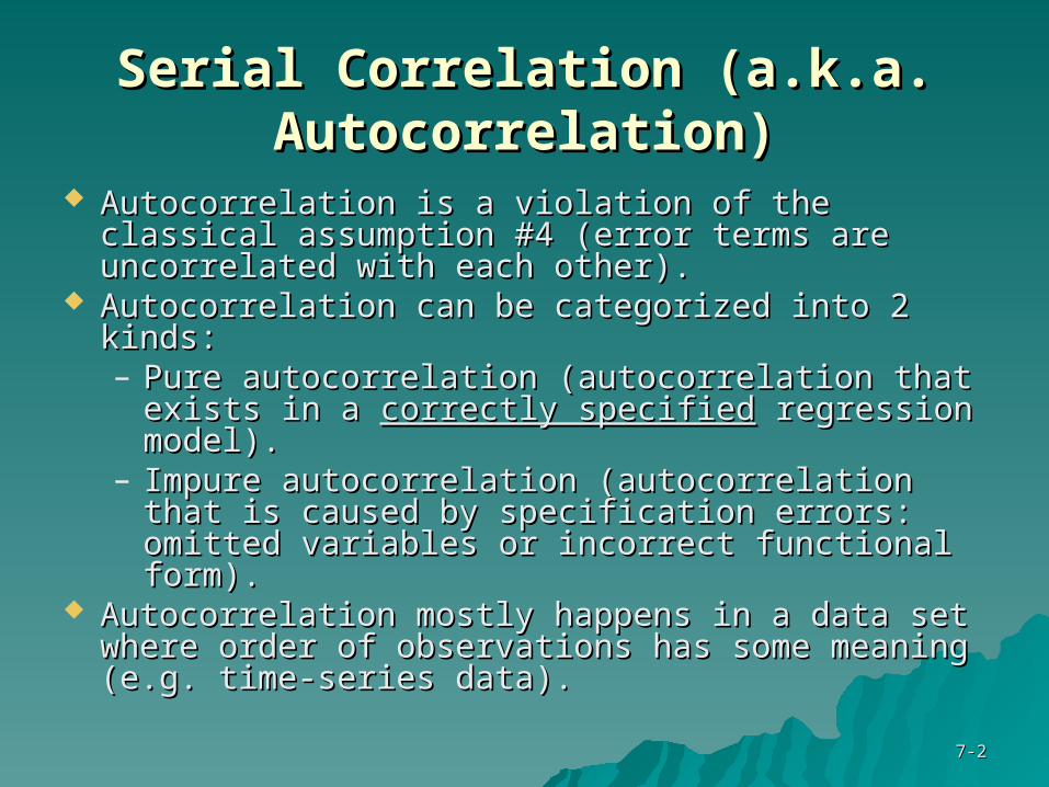
Serial Correlation (a.k.a. Autocorrelation)Serial Correlation (a.k.a. Autocorrelation)

Autocorrelation is a violation of the classical Autocorrelation is a violation of the classical assumption #4 (error terms are uncorrelated with assumption #4 (error terms are uncorrelated with each other).each other).

Autocorrelation can be categorized into 2 kinds:Autocorrelation can be categorized into 2 kinds:– Pure autocorrelation (autocorrelation that Pure autocorrelation (autocorrelation that

exists in a exists in a correctly specifiedcorrectly specified regression regression model).model).

– Impure autocorrelation (autocorrelation that is Impure autocorrelation (autocorrelation that is caused by specification errors: omitted caused by specification errors: omitted variables or incorrect functional form).variables or incorrect functional form).

Autocorrelation mostly happens in a data set Autocorrelation mostly happens in a data set where order of observations has some meaning where order of observations has some meaning (e.g. time-series data).(e.g. time-series data).

7-7-33

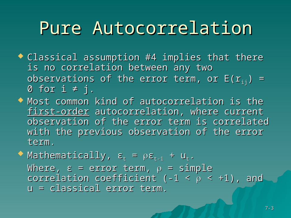
Pure AutocorrelationPure Autocorrelation

Classical assumption #4 implies that there is Classical assumption #4 implies that there is no correlation between any two observations no correlation between any two observations of the error term, or E(rof the error term, or E(rijij) = 0 for i ≠ j.) = 0 for i ≠ j.

Most common kind of autocorrelation is the Most common kind of autocorrelation is the first-orderfirst-order autocorrelation, where current autocorrelation, where current observation of the error term is correlated with observation of the error term is correlated with the previous observation of the error term.the previous observation of the error term.

Mathematically, Mathematically, εεtt = = εεt-1t-1 + u + utt..Where, Where, εε = error term, = error term, = simple correlation = simple correlation coefficient (-1 < coefficient (-1 < < +1), and u = classical < +1), and u = classical error term.error term.

7-7-44

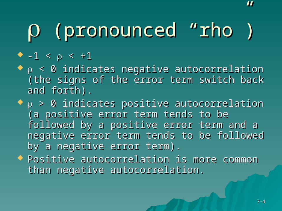
(pronounced “rho”)(pronounced “rho”) -1 < -1 < < +1 < +1 < 0 indicates negative autocorrelation (the < 0 indicates negative autocorrelation (the

signs of the error term switch back and forth).signs of the error term switch back and forth). > 0 indicates positive autocorrelation (a > 0 indicates positive autocorrelation (a

positive error term tends to be followed by a positive error term tends to be followed by a positive error term and a negative error term positive error term and a negative error term tends to be followed by a negative error tends to be followed by a negative error term).term).

Positive autocorrelation is more common than Positive autocorrelation is more common than negative autocorrelation.negative autocorrelation.

7-7-55

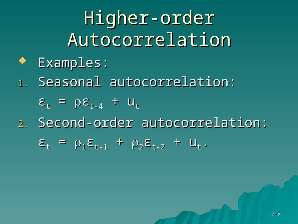
Higher-order AutocorrelationHigher-order Autocorrelation

Examples:Examples:

1.1. Seasonal autocorrelation:Seasonal autocorrelation:

εεtt = = εεt-4t-4 + u + utt

2.2. Second-order autocorrelation:Second-order autocorrelation:

εεtt = = 11εεt-1t-1 + + 22εεt-2t-2 + u + utt..

7-7-66

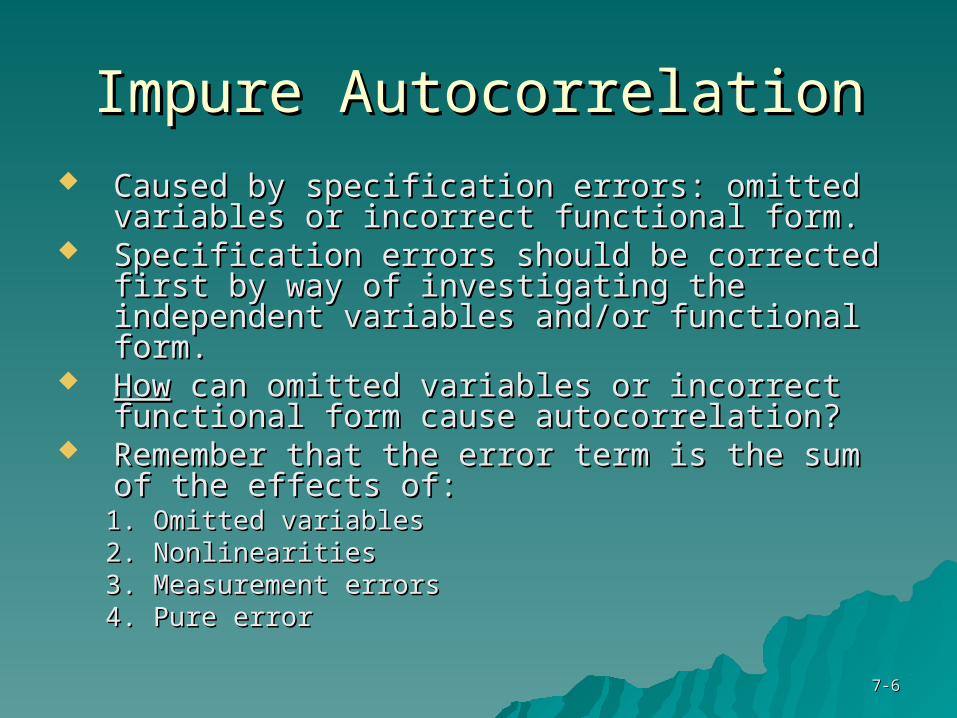
Impure AutocorrelationImpure Autocorrelation Caused by specification errors: omitted variables Caused by specification errors: omitted variables

or incorrect functional form.or incorrect functional form. Specification errors should be corrected first by Specification errors should be corrected first by

way of investigating the independent variables way of investigating the independent variables and/or functional form.and/or functional form.

HowHow can omitted variables or incorrect can omitted variables or incorrect functional form cause autocorrelation?functional form cause autocorrelation?

Remember that the error term is the sum of the Remember that the error term is the sum of the effects of:effects of:1.1. Omitted variablesOmitted variables2.2. NonlinearitiesNonlinearities3.3. Measurement errorsMeasurement errors4.4. Pure errorPure error

7-7-77

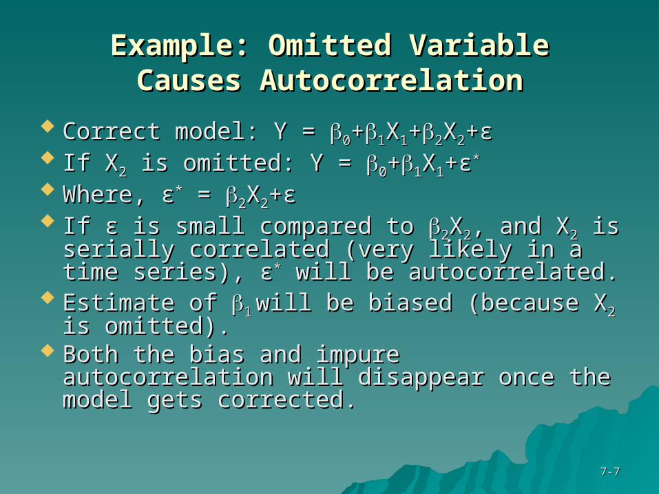
Example: Omitted VariableExample: Omitted VariableCauses AutocorrelationCauses Autocorrelation

Correct model: Y = Correct model: Y = 00++11XX11++22XX22++εε If XIf X22 is omitted: Y = is omitted: Y = 00++11XX11++εε**

Where, Where, εε** = = 22XX22++εε If If εε is small compared to is small compared to 22XX22, and X, and X22 is is

serially correlated (very likely in a time serially correlated (very likely in a time series), series), εε** will be autocorrelated. will be autocorrelated.

Estimate of Estimate of 11 will be biased (because Xwill be biased (because X22 is is omitted).omitted).

Both the bias and impure autocorrelation Both the bias and impure autocorrelation will disappear once the model gets will disappear once the model gets corrected.corrected.

7-7-88

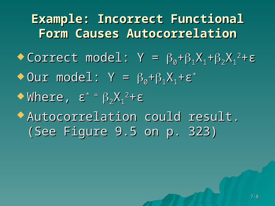
Example: Incorrect Functional Form Example: Incorrect Functional Form Causes AutocorrelationCauses Autocorrelation

Correct model: Y = Correct model: Y = 00++11XX11++22XX1122++εε

Our model: Y = Our model: Y = 00++11XX11++εε**

Where, Where, εε* = * = 22XX1122++εε

Autocorrelation could result. (See Autocorrelation could result. (See Figure 9.5 on p. 323)Figure 9.5 on p. 323)

7-7-99

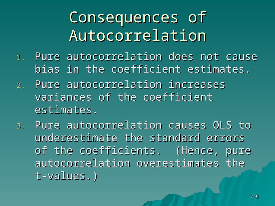
Consequences of AutocorrelationConsequences of Autocorrelation

1.1. Pure autocorrelation does not cause bias Pure autocorrelation does not cause bias in the coefficient estimates.in the coefficient estimates.

2.2. Pure autocorrelation increases variances Pure autocorrelation increases variances of the coefficient estimates.of the coefficient estimates.

3.3. Pure autocorrelation causes OLS to Pure autocorrelation causes OLS to underestimate the standard errors of the underestimate the standard errors of the coefficients. (Hence, pure coefficients. (Hence, pure autocorrelation overestimates the t-autocorrelation overestimates the t-values.)values.)

7-7-1010

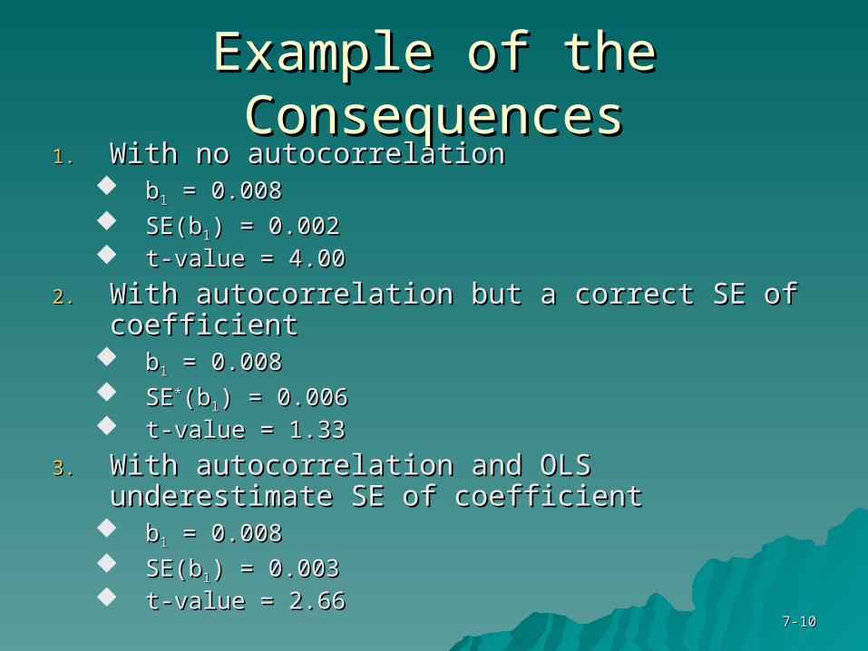
Example of the ConsequencesExample of the Consequences1.1. With no autocorrelationWith no autocorrelation

bb11 = 0.008 = 0.008 SE(bSE(b11) = 0.002) = 0.002 t-value = 4.00t-value = 4.00

2.2. With autocorrelation but a correct SE of With autocorrelation but a correct SE of coefficientcoefficient

bb11 = 0.008 = 0.008 SESE**(b(b11) = 0.006) = 0.006 t-value = 1.33t-value = 1.33

3.3. With autocorrelation and OLS underestimate SE With autocorrelation and OLS underestimate SE of coefficientof coefficient

bb11 = 0.008 = 0.008 SE(bSE(b11) = 0.003) = 0.003 t-value = 2.66t-value = 2.66

7-7-1111

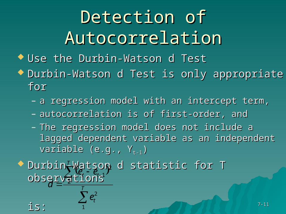
Detection of AutocorrelationDetection of Autocorrelation

Use the Durbin-Watson d TestUse the Durbin-Watson d Test Durbin-Watson d Test is only appropriate forDurbin-Watson d Test is only appropriate for

– a regression model with an intercept term,a regression model with an intercept term,– autocorrelation is of first-order, andautocorrelation is of first-order, and– The regression model does not include a lagged The regression model does not include a lagged

dependent variable as an independent variable dependent variable as an independent variable (e.g., Y(e.g., Yt-1t-1))

Durbin-Watson d statistic for T observationsDurbin-Watson d statistic for T observations

is:is:

T

t

T

tt

e

eed

1

2

2

21

7-7-1212

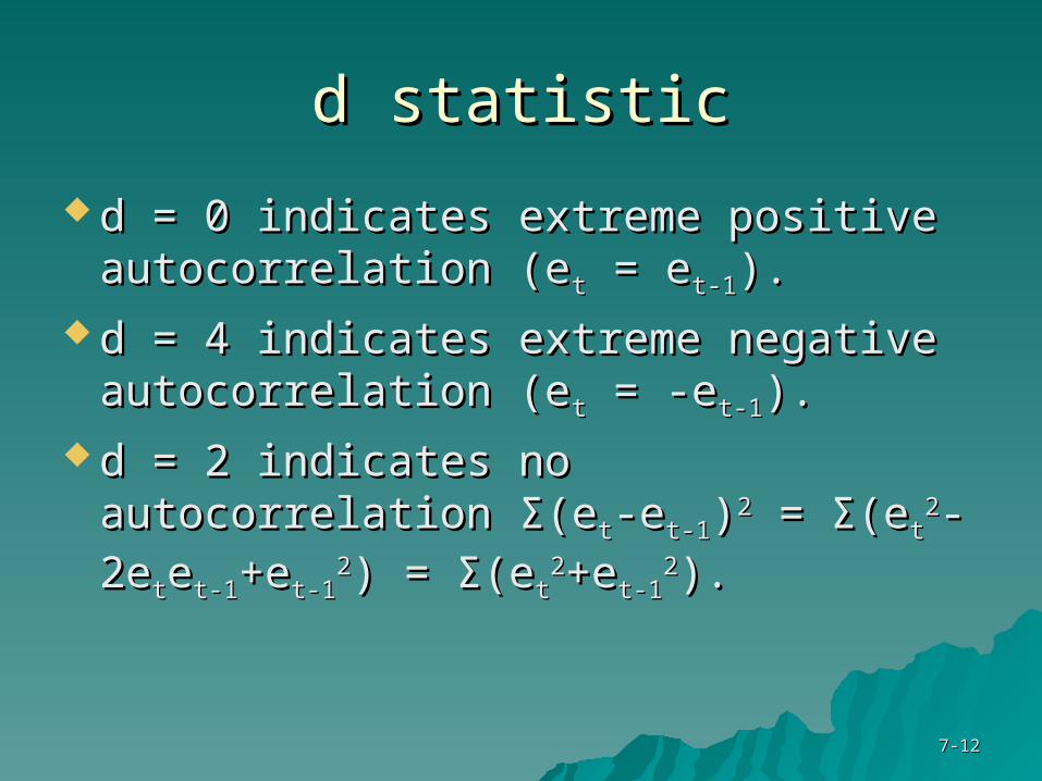
d statisticd statistic

d = 0 indicates extreme positive d = 0 indicates extreme positive autocorrelation (eautocorrelation (ett = e = et-1t-1).).

d = 4 indicates extreme negative d = 4 indicates extreme negative autocorrelation (eautocorrelation (ett = -e = -et-1t-1).).

d = 2 indicates no autocorrelation d = 2 indicates no autocorrelation ΣΣ(e(ett-e-et-1t-1))22 = = ΣΣ(e(ett

22-2e-2etteet-1t-1+e+et-1t-122) = ) =

ΣΣ(e(ett22+e+et-1t-1

22).).

7-7-1313

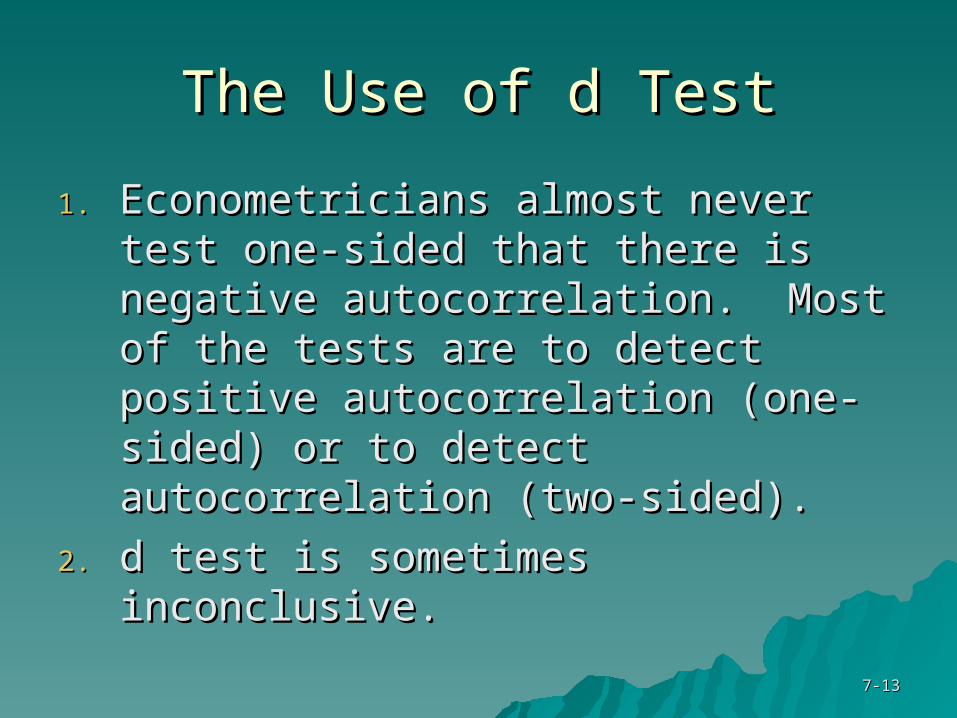
The Use of d TestThe Use of d Test

1.1. Econometricians almost never test Econometricians almost never test one-sided that there is negative one-sided that there is negative autocorrelation. Most of the tests autocorrelation. Most of the tests are to detect positive are to detect positive autocorrelation (one-sided) or to autocorrelation (one-sided) or to detect autocorrelation (two-sided).detect autocorrelation (two-sided).

2.2. d test is sometimes inconclusive.d test is sometimes inconclusive.

7-7-1414

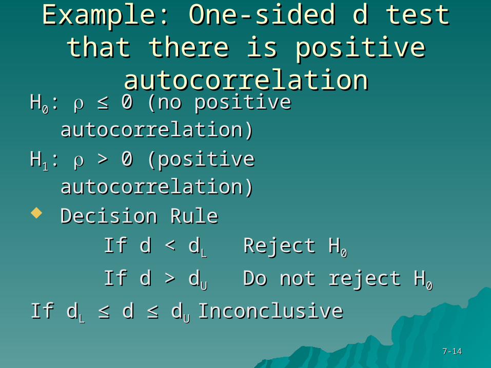
Example: One-sided d test that Example: One-sided d test that there is positive autocorrelationthere is positive autocorrelation

HH00: : ≤ 0 (no positive autocorrelation) ≤ 0 (no positive autocorrelation)

HH11: : > 0 (positive autocorrelation) > 0 (positive autocorrelation) Decision RuleDecision Rule

If d < dIf d < dLL Reject HReject H00

If d > dIf d > dUU Do not reject HDo not reject H00

If dIf dLL ≤ d ≤ d ≤ d ≤ dUU InconclusiveInconclusive

7-7-1515

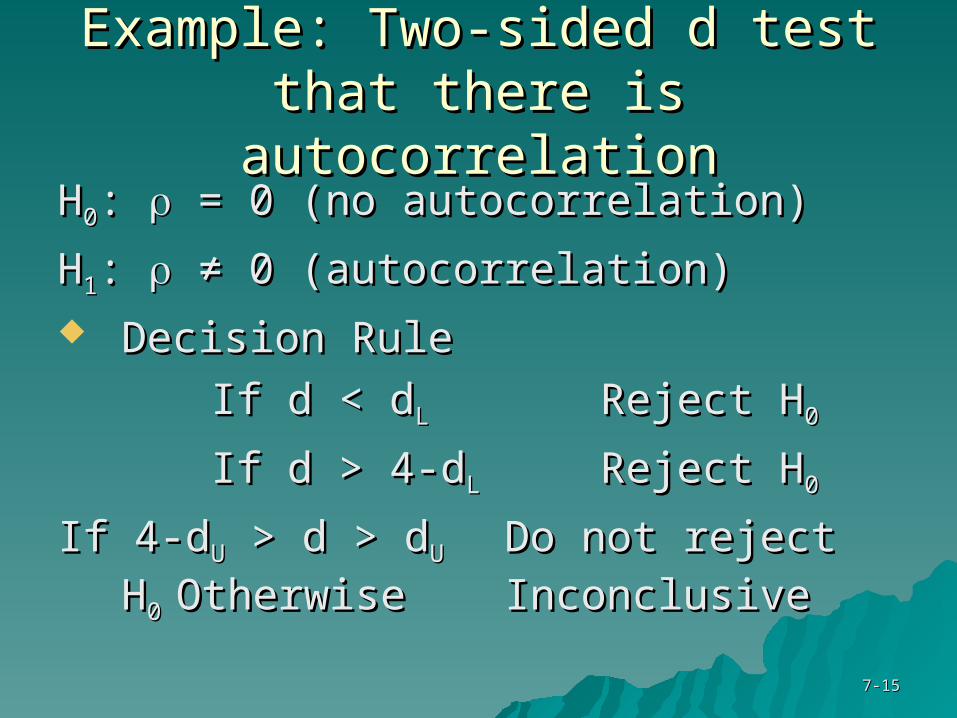
Example: Two-sided d test that Example: Two-sided d test that there is autocorrelationthere is autocorrelation

HH00: : = 0 (no autocorrelation) = 0 (no autocorrelation)

HH11: : ≠ 0 (autocorrelation) ≠ 0 (autocorrelation) Decision RuleDecision Rule

If d < dIf d < dLL Reject HReject H00

If d > 4-dIf d > 4-dLL Reject HReject H00

If 4-dIf 4-dUU > d > d > d > dUU Do not reject HDo not reject H0 0

OtherwiseOtherwise InconclusiveInconclusive

7-7-1616

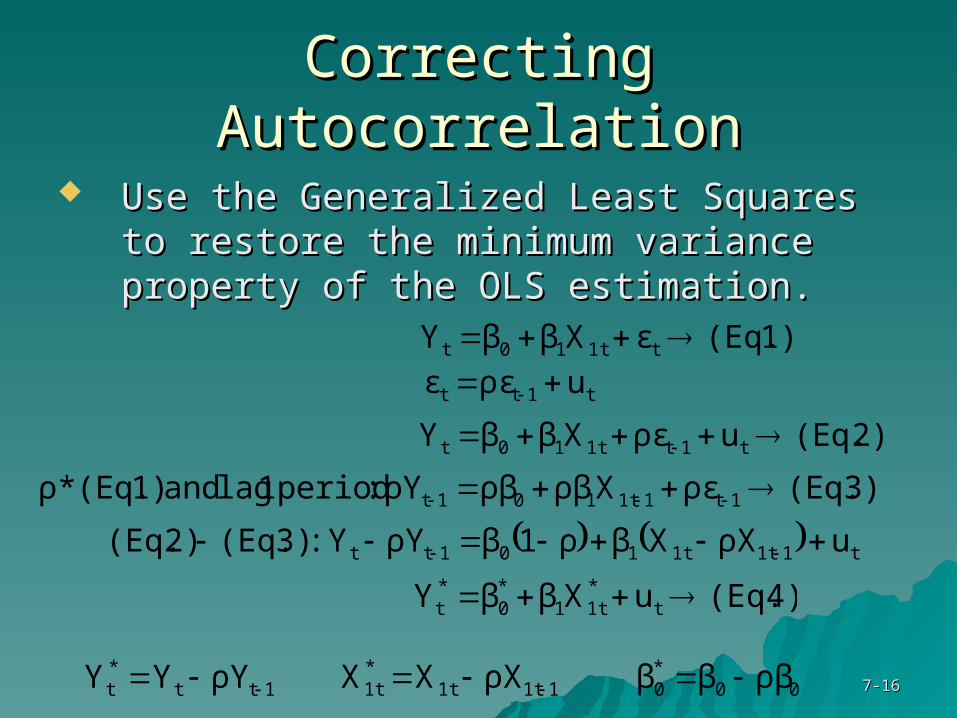
Correcting AutocorrelationCorrecting Autocorrelation

Use the Generalized Least Squares to Use the Generalized Least Squares to restore the minimum variance property restore the minimum variance property of the OLS estimation.of the OLS estimation.

1) (Eq.εXββY t1t10t

t1tt uρεε

2) (Eq.uρεXββY t1t1t10t

3) (Eq.ρεXρβρβρY :period 1 lag and 1) (Eq.*ρ 1t11t101t

t11t1t101tt uρXXβρ1βρYY :3) (Eq.2) (Eq.

4) (Eq.uXββY t*1t1

*0

*t

1tt*t ρYYY 11t1t

*1t ρXXX 00

*0 ρβββ

7-7-1717

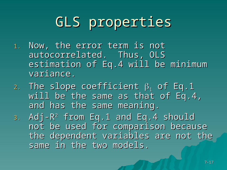
GLS propertiesGLS properties

1.1. Now, the error term is not Now, the error term is not autocorrelated. Thus, OLS estimation of autocorrelated. Thus, OLS estimation of Eq.4 will be minimum variance.Eq.4 will be minimum variance.

2.2. The slope coefficient The slope coefficient 11 of Eq.1 will be the of Eq.1 will be the same as that of Eq.4, and has the same same as that of Eq.4, and has the same meaning.meaning.

3.3. Adj-RAdj-R22 from Eq.1 and Eq.4 should not be from Eq.1 and Eq.4 should not be used for comparison because the used for comparison because the dependent variables are not the same in dependent variables are not the same in the two models.the two models.

7-7-1818

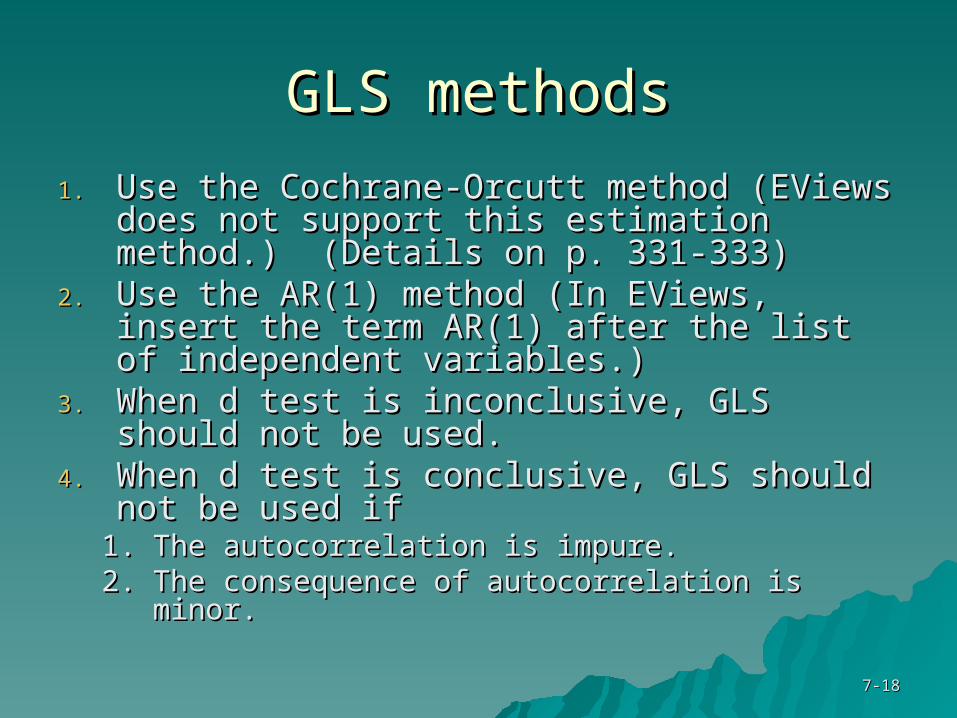
GLS methodsGLS methods

1.1. Use the Cochrane-Orcutt method (EViews Use the Cochrane-Orcutt method (EViews does not support this estimation does not support this estimation method.) (Details on p. 331-333)method.) (Details on p. 331-333)

2.2. Use the AR(1) method (In EViews, insert Use the AR(1) method (In EViews, insert the term AR(1) after the list of the term AR(1) after the list of independent variables.)independent variables.)

3.3. When d test is inconclusive, GLS should When d test is inconclusive, GLS should not be used.not be used.

4.4. When d test is conclusive, GLS should not When d test is conclusive, GLS should not be used ifbe used if

1.1. The autocorrelation is impure.The autocorrelation is impure.2.2. The consequence of autocorrelation is minor.The consequence of autocorrelation is minor.

7-7-1919

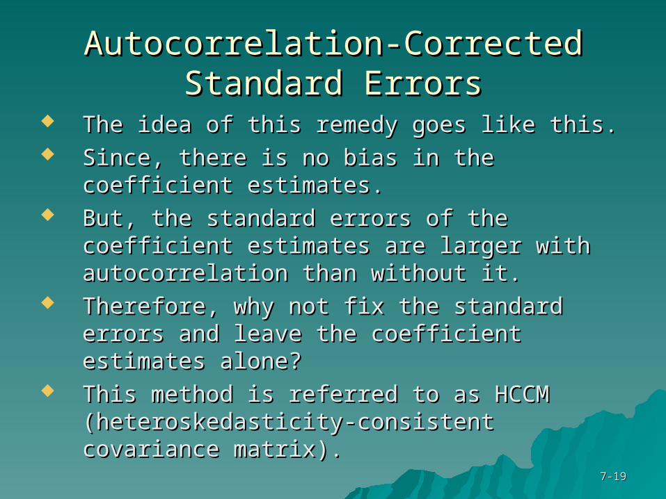
Autocorrelation-Corrected Standard ErrorsAutocorrelation-Corrected Standard Errors

The idea of this remedy goes like this.The idea of this remedy goes like this. Since, there is no bias in the coefficient Since, there is no bias in the coefficient

estimates.estimates. But, the standard errors of the coefficient But, the standard errors of the coefficient

estimates are larger with autocorrelation estimates are larger with autocorrelation than without it.than without it.

Therefore, why not fix the standard errors Therefore, why not fix the standard errors and leave the coefficient estimates alone?and leave the coefficient estimates alone?

This method is referred to as HCCM This method is referred to as HCCM (heteroskedasticity-consistent covariance (heteroskedasticity-consistent covariance matrix).matrix).

7-7-2020

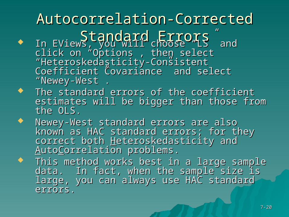
Autocorrelation-Corrected Standard ErrorsAutocorrelation-Corrected Standard Errors In EViews, you will choose “LS” and click on In EViews, you will choose “LS” and click on

“Options”, then select “Heteroskedasticity-“Options”, then select “Heteroskedasticity-Consistent Coefficient Covariance” and Consistent Coefficient Covariance” and select “Newey-West”.select “Newey-West”.

The standard errors of the coefficient The standard errors of the coefficient estimates will be bigger than those from the estimates will be bigger than those from the OLS.OLS.

Newey-West standard errors are also known Newey-West standard errors are also known as HAC standard errors; for they correct as HAC standard errors; for they correct both both HHeteroskedasticity and eteroskedasticity and AAutoutoCCorrelation orrelation problems.problems.

This method works best in a large sample This method works best in a large sample data. In fact, when the sample size is large, data. In fact, when the sample size is large, you can always use HAC standard errors.you can always use HAC standard errors.