Embed Size (px)
Citation preview

Metro MiningBauxite Hills Project
Environmental Impact Statement
Metro MiningChapter 21 - References
Environmental Impact Statement
Metro MiningAppendix J - BathymetricSurvey Report – Skardon River
Contract number: 20150303
Document name: Survey Report – Skardon River April 2015
Company Document No.: AI2015-MM-04-002 Security Classification: Business - Commercially in confidence
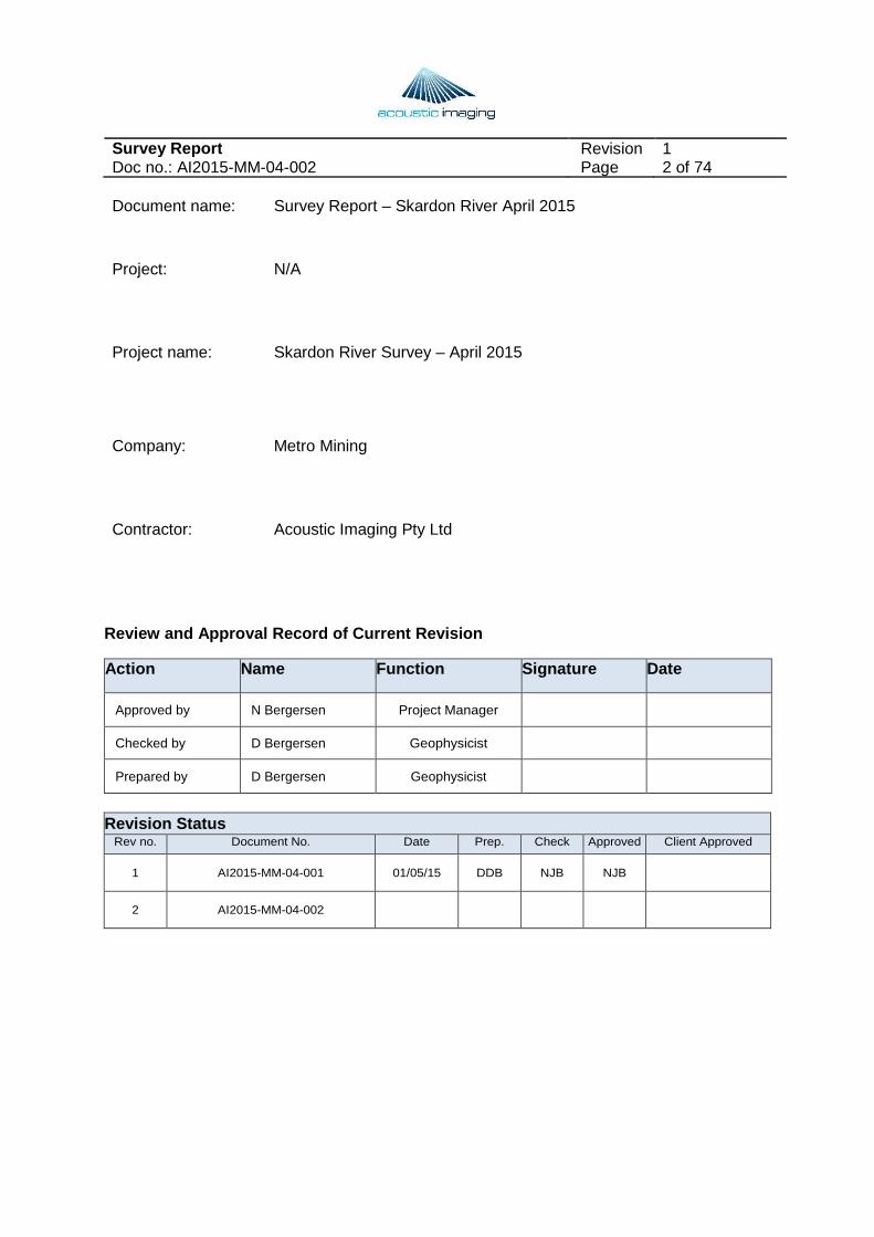
Survey Report Revision 1 Doc no.: AI2015-MM-04-002 Page 2 of 74
Document name: Survey Report – Skardon River April 2015
Project: N/A
Project name: Skardon River Survey – April 2015
Company: Metro Mining
Contractor: Acoustic Imaging Pty Ltd
Review and Approval Record of Current Revision
Revision Status Rev no. Document No. Date Prep. Check Approved Client Approved
1 AI2015-MM-04-001 01/05/15 DDB NJB NJB
2 AI2015-MM-04-002
Action Name Function Signature Date
Approved by N Bergersen Project Manager
Checked by D Bergersen Geophysicist
Prepared by D Bergersen Geophysicist
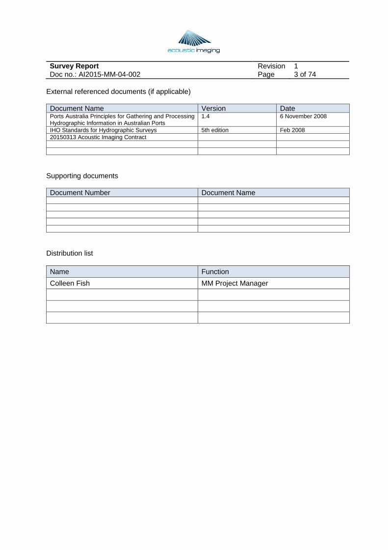
Survey Report Revision 1 Doc no.: AI2015-MM-04-002 Page 3 of 74
External referenced documents (if applicable)
Document Name Version Date Ports Australia Principles for Gathering and Processing Hydrographic Information in Australian Ports
1.4 6 November 2008
IHO Standards for Hydrographic Surveys 5th edition Feb 2008 20150313 Acoustic Imaging Contract
Supporting documents
Document Number Document Name
Distribution list
Name Function
Colleen Fish MM Project Manager
Survey Report Revision 1 Doc no.: AI2015-MM-04-002 Page 4 of 74
Contents
Abbreviations and definitions ................................................................................................. 5Definitions within the contract ................................................................................................ 61. Introduction .................................................................................................................. 7
1.1 Reason for issue ..................................................................................................... 91.2 Survey Details ......................................................................................................... 91.3 Survey Standard ..................................................................................................... 9
2 Geodetic Parameters and Reference Levels ..................................................................102.1 Units .......................................................................................................................102.2 GNSS and Positioning systems ..............................................................................102.3 Geoid Model; Ellipsoids and Geoids .......................................................................102.4 Geodetic Parameters and Real time Geodetic configuration ..................................122.5 Reference Levels/Datum ........................................................................................13
3 Equipment......................................................................................................................143.1 Survey Vessel and Sensors ...................................................................................14
4 Testing and Calibration ..................................................................................................234.1 Benchmark Checks ................................................................................................234.2 Data Reduction ......................................................................................................244.3 Field Checks ..........................................................................................................27
4.3.1 Position / Orientation System Calibration ..........................................................274.3.2 Multi Beam Echo Sounder System Calibration (Patch test) ...............................314.3.3 Speed of sound establishment ..........................................................................31
5 Acquisition and Processing ............................................................................................325.1 Data Acquisition .....................................................................................................325.2 Acquisition Issues and Modifications ......................................................................325.3 Survey Reporting ...................................................................................................365.4 Data Processing .....................................................................................................365.5 Software packages .................................................................................................40
6 Interpretation and Results ..............................................................................................416.1 Section 0 ................................................................................................................416.2 Section 1 ................................................................................................................456.3 Section 2 ................................................................................................................486.4 Section 3 ................................................................................................................516.5 Section 4 ................................................................................................................546.6 Section 5 ................................................................................................................586.7 Section 6 ................................................................................................................64
7 Results and Recommendations .....................................................................................667.1 Current Geodetic Control .......................................................................................667.2 Future Horizontal and Vertical Control ....................................................................677.3 Relationship between 2009 Chart Soundings and 2015 Bathymetry ......................68
8 Summary .......................................................................................................................74Appendices ..........................................................................................................................75

Survey Report Revision 1 Doc no.: AI2015-MM-04-002 Page 5 of 74
Abbreviations and definitions
Abbreviation Written in full Additional explanationAHD Australian Height Datum Terrestrial Height Datum AUSPOS Online GPS data processing
facility provided by Geoscience Australia
AUSPOS generates GDA94 coordinates from raw GPS logging.
BM Bench Mark A topographic control station with known position, elevation, or both position and elevation.
CD Chart datum Is the height reference used in hydrography
DGPS Differential GPS Enhancement to the 2-dimensional accuracy of GPS (sub-meter accurate)
GDA94 Geocentric Datum of Australia 1994
The geographic grid in use at the Project
GPS Global Positioning System Navigational aid through satellites; typical accuracy 2-5 meter
GRS80 Geodetic Reference System 1980
Ellipsoid used for GDA94 system
LAT Lowest Astronomical Tide The lowest level which can be predicted to occur under average meteorological conditions. The Hydrographic Service of the Royal Australian Navy has adopted LAT as Chart Datum.
MGA94 Map Grid of Australia 1994 Metric coordinate grid based on Transverse Mercator Projection of GDA94 coordinates.
RTK Real Time Kinematics Enhancement to the 3-dimensional accuracy of GPS (cm accuracy)
TBM Temporary Benchmark Benchmark generated during the project and in use for project purpose only.
WGS84 World Geodetic System 1984 Geodetic coordinate system, used by GPS.
Survey Report Revision 1 Doc no.: AI2015-MM-04-002 Page 6 of 74
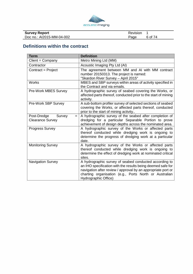
Definitions within the contract
Term Definition Client = Company Metro Mining Ltd (MM) Contractor Acoustic Imaging Pty Ltd (AI) Contract = Project The agreement between MM and AI with MM contract
number 20150313. The project is named: "Skardon River Survey – April 2015"
Works MBES and SBP surveys within areas of activity specified in the Contract and via emails.
Pre-Work MBES Survey A hydrographic survey of seabed covering the Works, or affected parts thereof, conducted prior to the start of mining activity.
Pre-Work SBP Survey A sub-bottom profiler survey of selected sections of seabed covering the Works, or affected parts thereof, conducted prior to the start of mining activity..
Post-Dredge Survey = Clearance Survey
A hydrographic survey of the seabed after completion of dredging for a particular Separable Portion to prove achievement of design depths across the nominated area.
Progress Survey A hydrographic survey of the Works or affected parts thereof conducted while dredging work is ongoing to determine the progress of dredging work at a particular date.
Monitoring Survey A hydrographic survey of the Works or affected parts thereof conducted while dredging work is ongoing to determine the effect of dredging work at nominated critical sites.
Navigation Survey A hydrographic survey of seabed conducted according to an IHO specification with the results being deemed safe for navigation after review / approval by an appropriate port or charting organisation (e.g., Ports North or Australian Hydrographic Office)

Survey Report Revision 1 Doc no.: AI2015-MM-04-002 Page 7 of 74
1. Introduction
Cape Alumina Ltd (MM) contracted Acoustic Imaging Pty Ltd (AI) to acquire, process, and interpret a multibeam echo sounder (MBES) and sub-bottom profiler (SBP) data set inside and outside the Skardon River in Far North Queensland.
The Skardon River is located on the western side of the Cape York Peninsula, approximately 100km north of Weipa. Mobilisation and survey activities occurred between April 9-23, 2015.
The purpose of the survey was two-fold. First, to provide baseline bathymetry reduced to the currently understood Lowest Astronomical Tide (LAT) datum within the Skardon River, and second, to assess sediment thickness across three areas where additional engineering or dredging work was proposed for barge loading or navigation.
The MBES survey area extended from the proposed Cape Alumina barge loading facility in the upper reaches of the Skardon River out to 6km offshore along the current navigation channel leading into the Skardon River (Figure 1).
Figure 1: Proposed area for MBES survey coverage. Orange polygon shows 200m buffer zone provided by Cape Alumina.

Survey Report Revision 1 Doc no.: AI2015-MM-04-002 Page 8 of 74
SBP surveying occurred across three areas. The first lay within the channel leading into the Skardon Channel (Figure 2). The other areas were farther upstream, around the current barge berthing area and upriver to a proposed barge loading facility yet to be built (Figure 3).
Figure 2: Proposed area for SBP survey coverage in the Skardon River channel. 25m buffer zone provided by Cape Alumina shown in yellow.
Figure 3: Proposed area for SBP survey coverage across the two barge loading facilities in the upper reaches of the Skardon River.
Survey Report Revision 1 Doc no.: AI2015-MM-04-002 Page 9 of 74
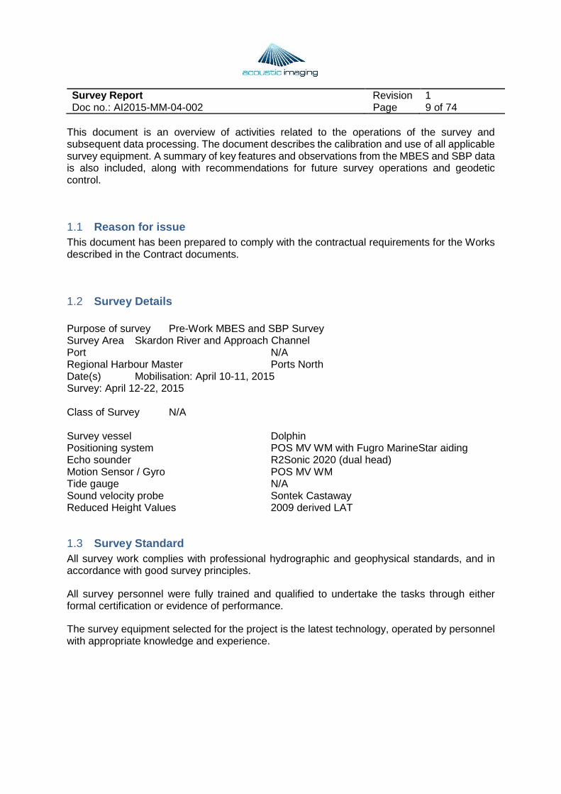
This document is an overview of activities related to the operations of the survey and subsequent data processing. The document describes the calibration and use of all applicable survey equipment. A summary of key features and observations from the MBES and SBP data is also included, along with recommendations for future survey operations and geodetic control.
1.1 Reason for issue This document has been prepared to comply with the contractual requirements for the Works described in the Contract documents.
1.2 Survey Details Purpose of survey Pre-Work MBES and SBP Survey Survey Area Skardon River and Approach Channel Port N/A Regional Harbour Master Ports North Date(s) Mobilisation: April 10-11, 2015 Survey: April 12-22, 2015 Class of Survey N/A Survey vessel Dolphin Positioning system POS MV WM with Fugro MarineStar aiding Echo sounder R2Sonic 2020 (dual head) Motion Sensor / Gyro POS MV WM Tide gauge N/A Sound velocity probe Sontek Castaway Reduced Height Values 2009 derived LAT
1.3 Survey Standard All survey work complies with professional hydrographic and geophysical standards, and in accordance with good survey principles.
All survey personnel were fully trained and qualified to undertake the tasks through either formal certification or evidence of performance.
The survey equipment selected for the project is the latest technology, operated by personnel with appropriate knowledge and experience.
Survey Report Revision 1 Doc no.: AI2015-MM-04-002 Page 10 of 74
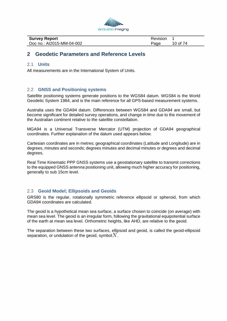
2 Geodetic Parameters and Reference Levels
2.1 Units All measurements are in the International System of Units.
2.2 GNSS and Positioning systems Satellite positioning systems generate positions to the WGS84 datum. WGS84 is the World Geodetic System 1984, and is the main reference for all GPS-based measurement systems.
Australia uses the GDA94 datum. Differences between WGS84 and GDA94 are small, but become significant for detailed survey operations, and change in time due to the movement of the Australian continent relative to the satellite constellation.
MGA94 is a Universal Transverse Mercator (UTM) projection of GDA94 geographical coordinates. Further explanation of the datum used appears below.
Cartesian coordinates are in metres; geographical coordinates (Latitude and Longitude) are in degrees, minutes and seconds; degrees minutes and decimal minutes or degrees and decimal degrees.
Real Time Kinematic PPP GNSS systems use a geostationary satellite to transmit corrections to the equipped GNSS antenna positioning unit, allowing much higher accuracy for positioning, generally to sub 15cm level.
2.3 Geoid Model; Ellipsoids and Geoids GRS80 is the regular, rotationally symmetric reference ellipsoid or spheroid, from which GDA94 coordinates are calculated.
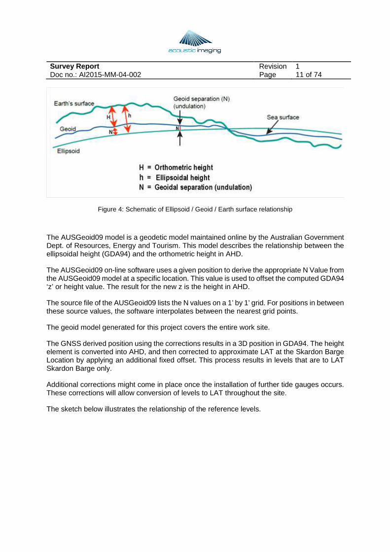
The geoid is a hypothetical mean sea surface, a surface chosen to coincide (on average) with mean sea level. The geoid is an irregular form, following the gravitational equipotential surface of the earth at mean sea level. Orthometric heights, like AHD, are relative to the geoid.
The separation between these two surfaces, ellipsoid and geoid, is called the geoid-ellipsoid separation, or undulation of the geoid, symbol .
Survey Report Revision 1 Doc no.: AI2015-MM-04-002 Page 11 of 74
Figure 4: Schematic of Ellipsoid / Geoid / Earth surface relationship
The AUSGeoid09 model is a geodetic model maintained online by the Australian Government Dept. of Resources, Energy and Tourism. This model describes the relationship between the ellipsoidal height (GDA94) and the orthometric height in AHD.
The AUSGeoid09 on-line software uses a given position to derive the appropriate N Value from the AUSGeoid09 model at a specific location. This value is used to offset the computed GDA94 ‘z’ or height value. The result for the new z is the height in AHD.
The source file of the AUSGeoid09 lists the N values on a 1’ by 1’ grid. For positions in between these source values, the software interpolates between the nearest grid points.
The geoid model generated for this project covers the entire work site.
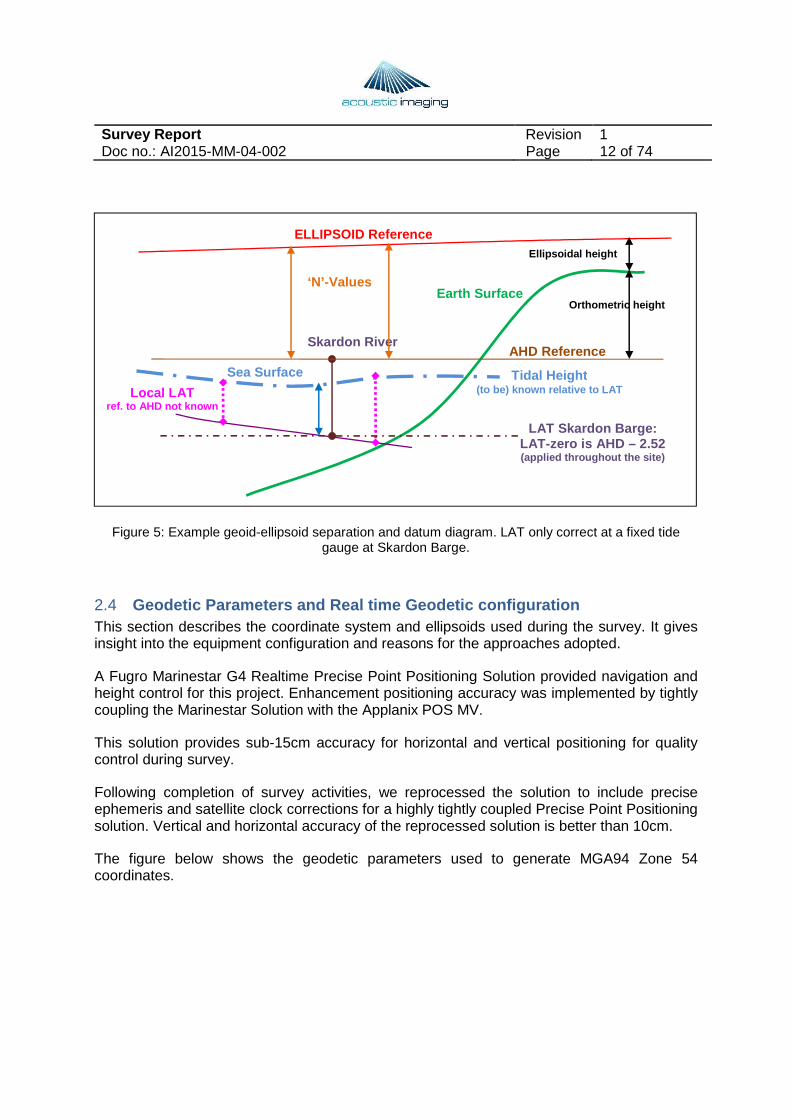
The GNSS derived position using the corrections results in a 3D position in GDA94. The height element is converted into AHD, and then corrected to approximate LAT at the Skardon Barge Location by applying an additional fixed offset. This process results in levels that are to LAT Skardon Barge only.
Additional corrections might come in place once the installation of further tide gauges occurs. These corrections will allow conversion of levels to LAT throughout the site.
The sketch below illustrates the relationship of the reference levels.
Survey Report Revision 1 Doc no.: AI2015-MM-04-002 Page 12 of 74
Figure 5: Example geoid-ellipsoid separation and datum diagram. LAT only correct at a fixed tide gauge at Skardon Barge.
2.4 Geodetic Parameters and Real time Geodetic configur ation This section describes the coordinate system and ellipsoids used during the survey. It gives insight into the equipment configuration and reasons for the approaches adopted.
A Fugro Marinestar G4 Realtime Precise Point Positioning Solution provided navigation and height control for this project. Enhancement positioning accuracy was implemented by tightly coupling the Marinestar Solution with the Applanix POS MV.
This solution provides sub-15cm accuracy for horizontal and vertical positioning for quality control during survey.
Following completion of survey activities, we reprocessed the solution to include precise ephemeris and satellite clock corrections for a highly tightly coupled Precise Point Positioning solution. Vertical and horizontal accuracy of the reprocessed solution is better than 10cm.
The figure below shows the geodetic parameters used to generate MGA94 Zone 54 coordinates.
ELLIPSOID Reference
Earth Surface
AHD Reference
LAT Skardon Barge : LAT-zero is AHD – 2.52 (applied throughout the site)
‘N’ -Values
Orthometric height
Skardon River
Ellipsoidal height
Tidal Height (to be) known relative to LAT
Sea Surface
Local LAT ref. to AHD not known

Survey Report Revision 1 Doc no.: AI2015-MM-04-002 Page 13 of 74
Figure 6: Transformation parameters for ITRF2000 to GDA94
Shift validity was determined for the epoch 17th April 2015.
These parameters were independently checked for accuracy in two different data transformation software packages.
For this project, the QINSy acquisition software computed the correction to GDA94, rather than to WGS84. This method ensured that no intermediate change of geodetic settings was required over the duration of the project.
2.5 Reference Levels/Datum For any survey, soundings and measurements are reduced to a vertical datum. All levels on drawings and in data sets are referenced to this datum.
The datum used for this project is LAT Skardon Barge, derived for Ports North during a 2009 survey. The LAT value is approximately 2.5 metres above the Australian Height Datum (AHD).
Survey Report Revision 1 Doc no.: AI2015-MM-04-002 Page 14 of 74
3 Equipment
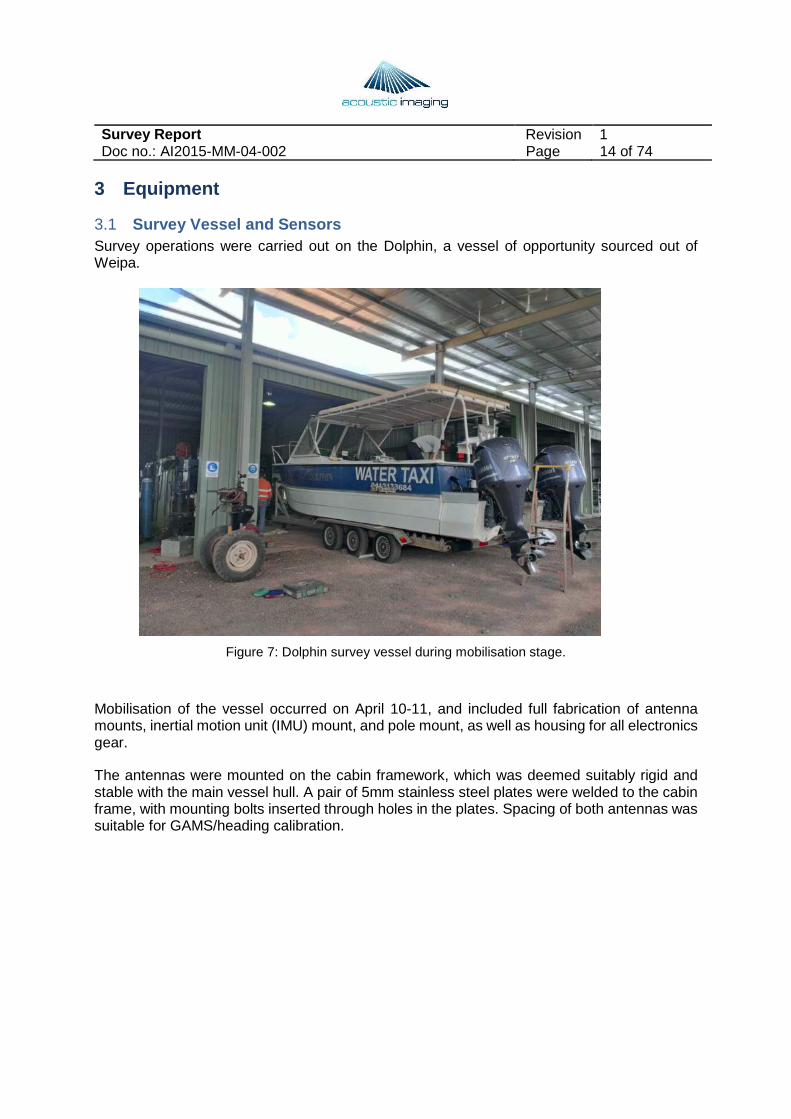
3.1 Survey Vessel and Sensors Survey operations were carried out on the Dolphin, a vessel of opportunity sourced out of Weipa.
Figure 7: Dolphin survey vessel during mobilisation stage.
Mobilisation of the vessel occurred on April 10-11, and included full fabrication of antenna mounts, inertial motion unit (IMU) mount, and pole mount, as well as housing for all electronics gear.
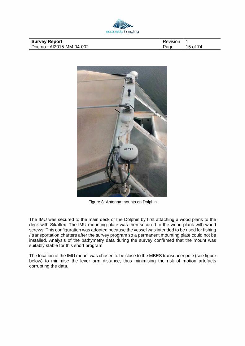
The antennas were mounted on the cabin framework, which was deemed suitably rigid and stable with the main vessel hull. A pair of 5mm stainless steel plates were welded to the cabin frame, with mounting bolts inserted through holes in the plates. Spacing of both antennas was suitable for GAMS/heading calibration.
Survey Report Revision 1 Doc no.: AI2015-MM-04-002 Page 15 of 74
Figure 8: Antenna mounts on Dolphin
The IMU was secured to the main deck of the Dolphin by first attaching a wood plank to the deck with Sikaflex. The IMU mounting plate was then secured to the wood plank with wood screws. This configuration was adopted because the vessel was intended to be used for fishing / transportation charters after the survey program so a permanent mounting plate could not be installed. Analysis of the bathymetry data during the survey confirmed that the mount was suitably stable for this short program.
The location of the IMU mount was chosen to be close to the MBES transducer pole (see figure below) to minimise the lever arm distance, thus minimising the risk of motion artefacts corrupting the data.
Survey Report Revision 1 Doc no.: AI2015-MM-04-002 Page 16 of 74
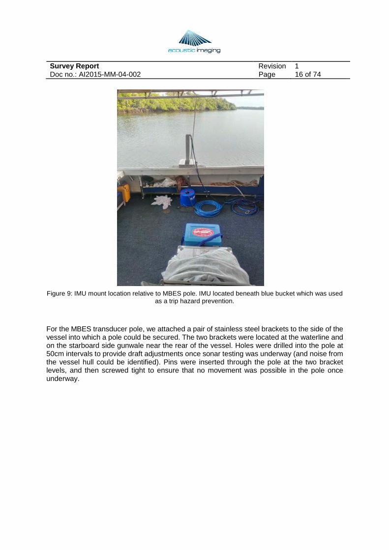
Figure 9: IMU mount location relative to MBES pole. IMU located beneath blue bucket which was used as a trip hazard prevention.
For the MBES transducer pole, we attached a pair of stainless steel brackets to the side of the vessel into which a pole could be secured. The two brackets were located at the waterline and on the starboard side gunwale near the rear of the vessel. Holes were drilled into the pole at 50cm intervals to provide draft adjustments once sonar testing was underway (and noise from the vessel hull could be identified). Pins were inserted through the pole at the two bracket levels, and then screwed tight to ensure that no movement was possible in the pole once underway.
Survey Report Revision 1 Doc no.: AI2015-MM-04-002 Page 17 of 74
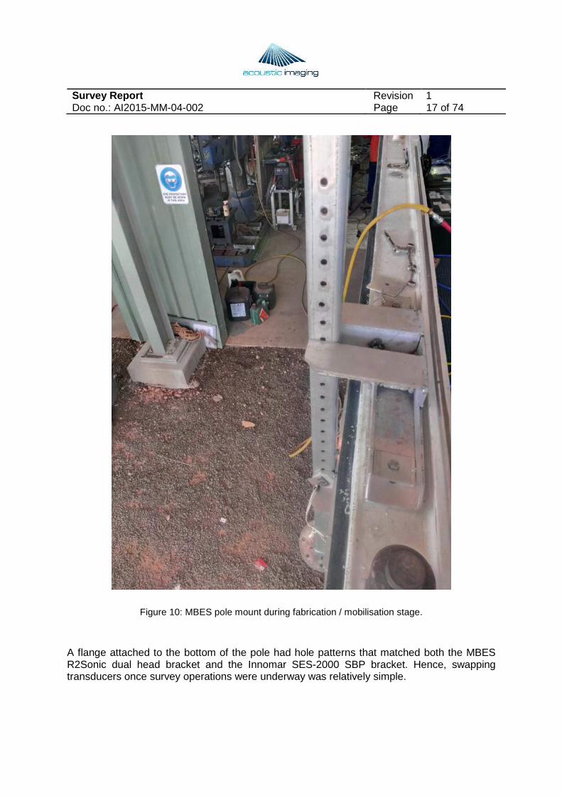
Figure 10: MBES pole mount during fabrication / mobilisation stage.
A flange attached to the bottom of the pole had hole patterns that matched both the MBES R2Sonic dual head bracket and the Innomar SES-2000 SBP bracket. Hence, swapping transducers once survey operations were underway was relatively simple.
Survey Report Revision 1 Doc no.: AI2015-MM-04-002 Page 18 of 74
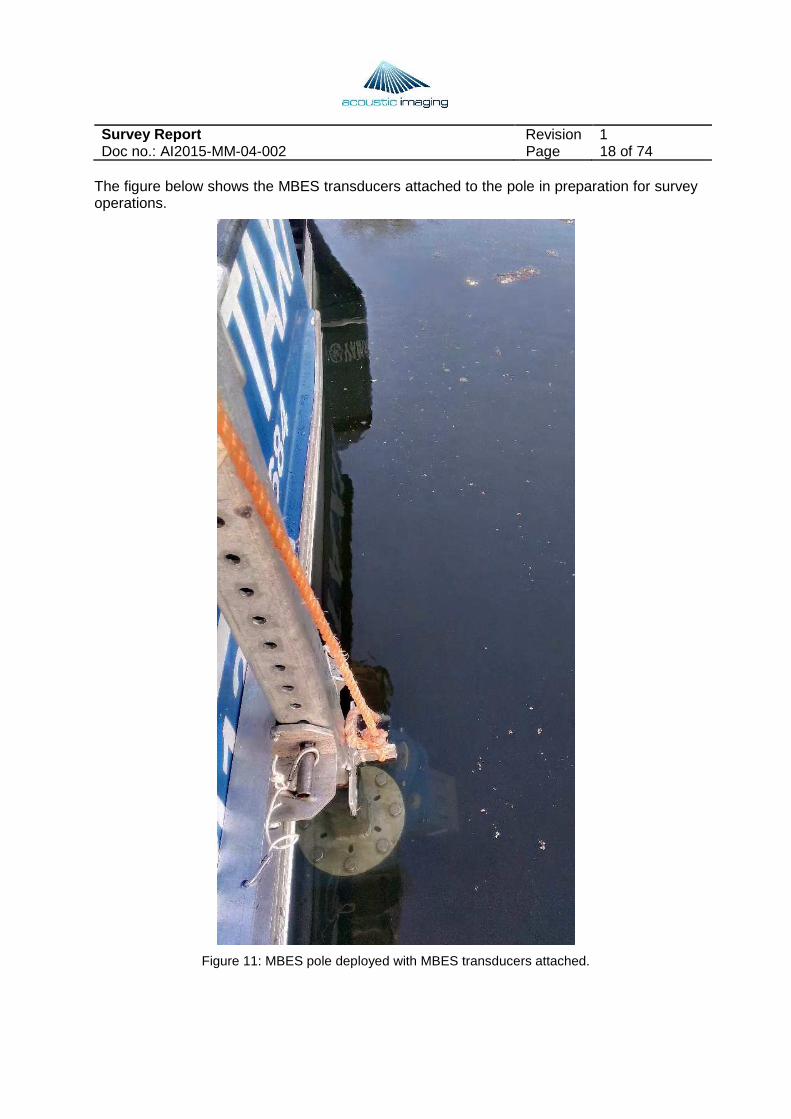
The figure below shows the MBES transducers attached to the pole in preparation for survey operations.
Figure 11: MBES pole deployed with MBES transducers attached.
Survey Report Revision 1 Doc no.: AI2015-MM-04-002 Page 19 of 74
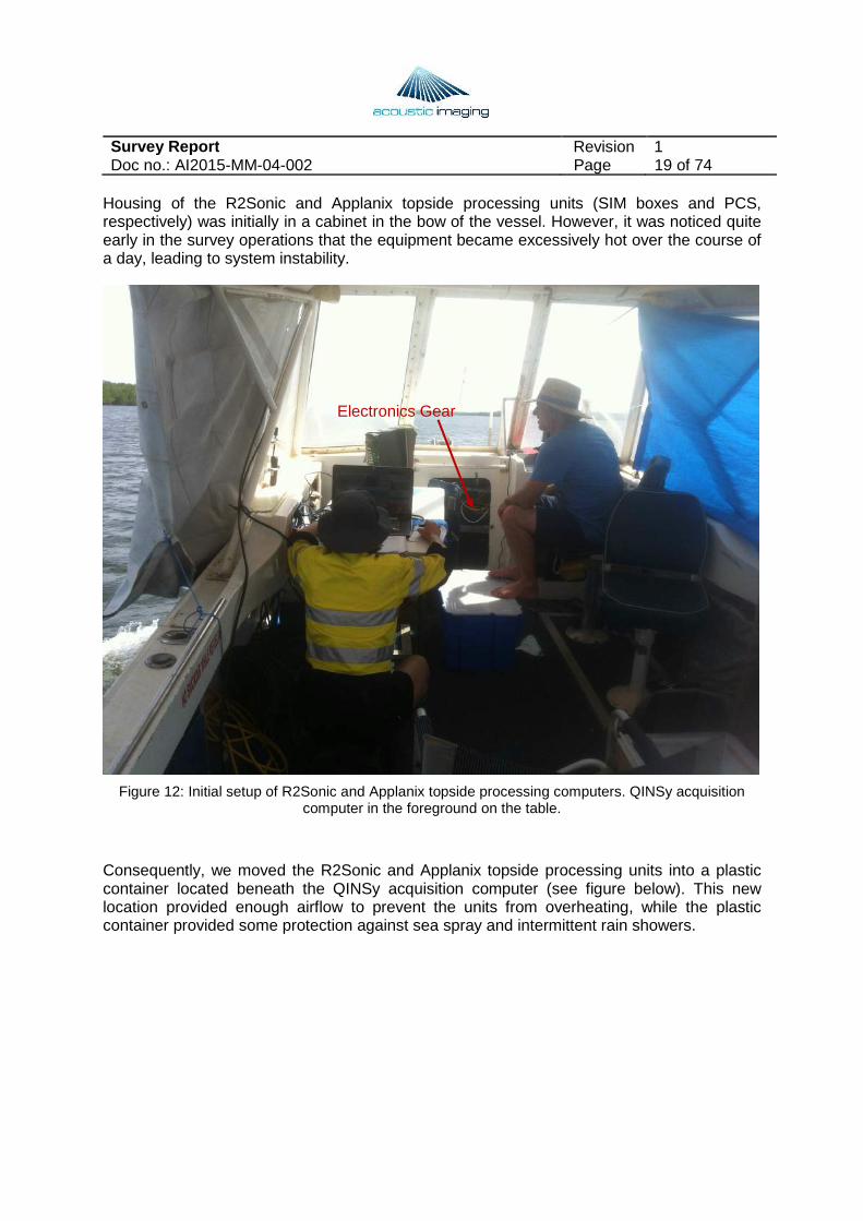
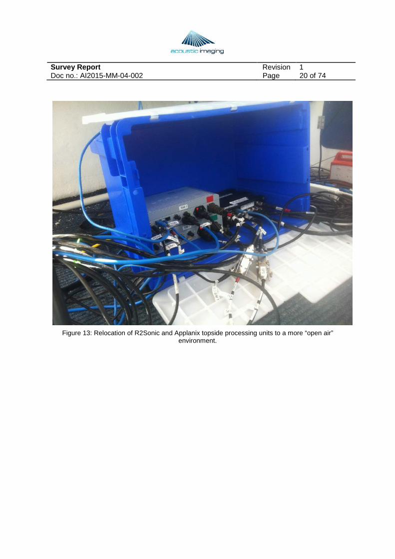
Housing of the R2Sonic and Applanix topside processing units (SIM boxes and PCS, respectively) was initially in a cabinet in the bow of the vessel. However, it was noticed quite early in the survey operations that the equipment became excessively hot over the course of a day, leading to system instability.
Figure 12: Initial setup of R2Sonic and Applanix topside processing computers. QINSy acquisition computer in the foreground on the table.
Consequently, we moved the R2Sonic and Applanix topside processing units into a plastic container located beneath the QINSy acquisition computer (see figure below). This new location provided enough airflow to prevent the units from overheating, while the plastic container provided some protection against sea spray and intermittent rain showers.
Electronics Gear
Survey Report Revision 1 Doc no.: AI2015-MM-04-002 Page 20 of 74
Figure 13: Relocation of R2Sonic and Applanix topside processing units to a more “open air” environment.
Survey Report Revision 1 Doc no.: AI2015-MM-04-002 Page 21 of 74
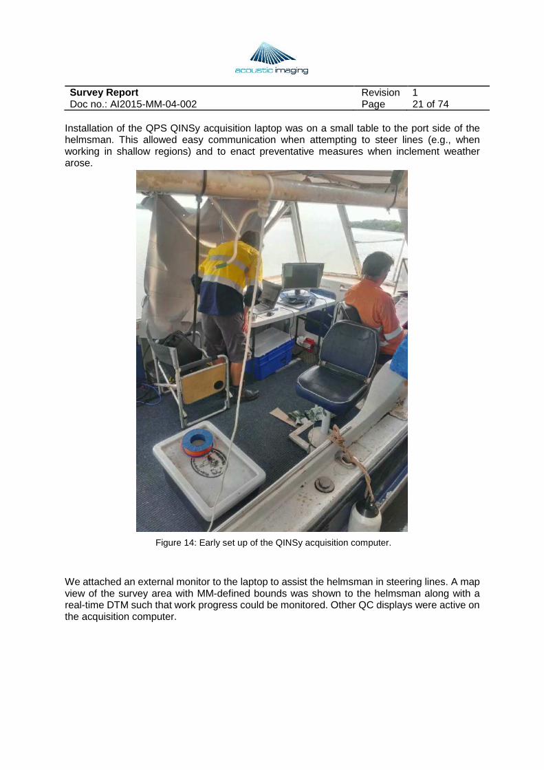
Installation of the QPS QINSy acquisition laptop was on a small table to the port side of the helmsman. This allowed easy communication when attempting to steer lines (e.g., when working in shallow regions) and to enact preventative measures when inclement weather arose.
Figure 14: Early set up of the QINSy acquisition computer.
We attached an external monitor to the laptop to assist the helmsman in steering lines. A map view of the survey area with MM-defined bounds was shown to the helmsman along with a real-time DTM such that work progress could be monitored. Other QC displays were active on the acquisition computer.
Survey Report Revision 1 Doc no.: AI2015-MM-04-002 Page 22 of 74
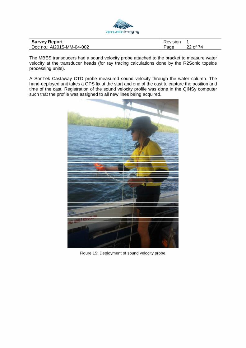
The MBES transducers had a sound velocity probe attached to the bracket to measure water velocity at the transducer heads (for ray tracing calculations done by the R2Sonic topside processing units).
A SonTek Castaway CTD probe measured sound velocity through the water column. The hand-deployed unit takes a GPS fix at the start and end of the cast to capture the position and time of the cast. Registration of the sound velocity profile was done in the QINSy computer such that the profile was assigned to all new lines being acquired.
Figure 15: Deployment of sound velocity probe.
Survey Report Revision 1 Doc no.: AI2015-MM-04-002 Page 23 of 74
4 Testing and Calibration All equipment in use on site had a valid test and calibration certificate and/or a validation sticker where applicable.
Upon completion of installation, we checked that baseline functionality of sensors and other equipment was acceptable. We conducted local calibrations and verifications where applicable. Field checks on equipment appear as Appendices in this document.
Survey operations were either suspended or moved to a more favourable location when weather conditions caused either degradation in data quality or endangered survey personnel or equipment.
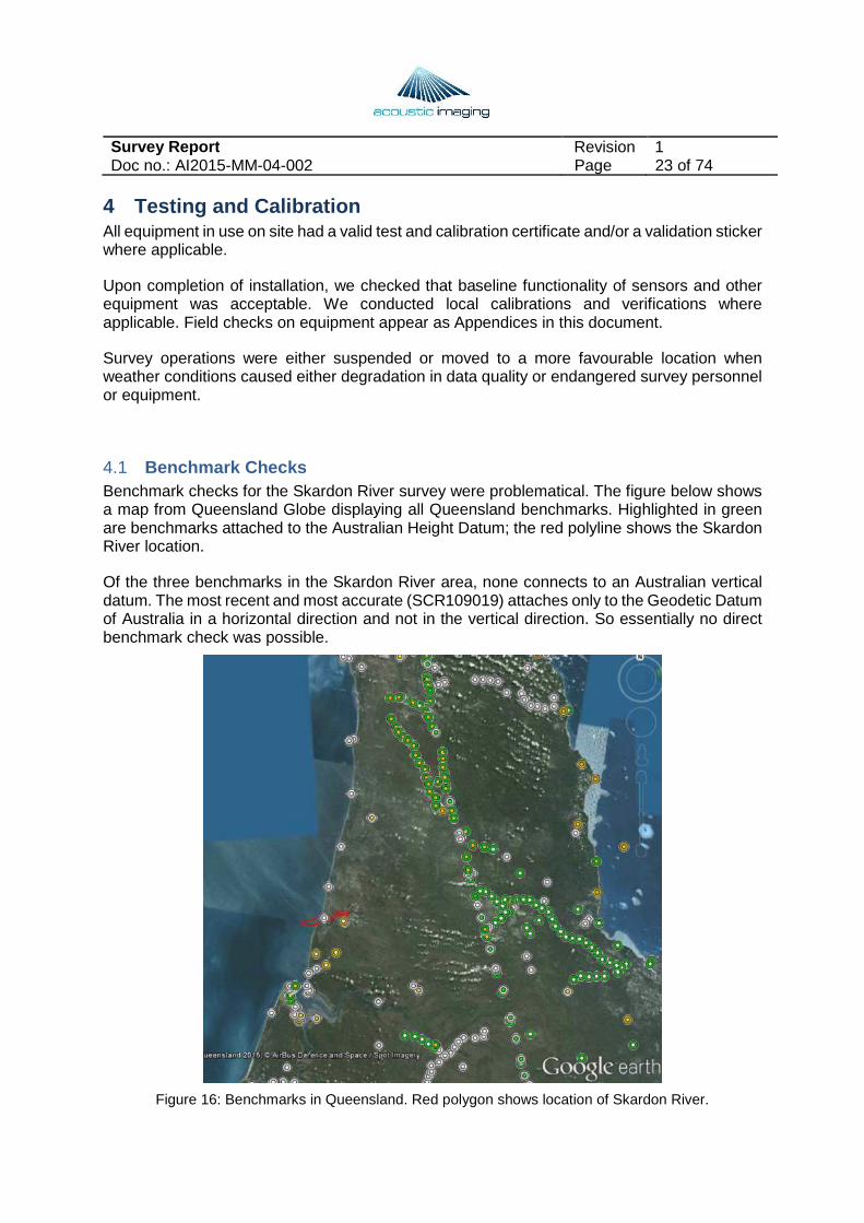
4.1 Benchmark Checks Benchmark checks for the Skardon River survey were problematical. The figure below shows a map from Queensland Globe displaying all Queensland benchmarks. Highlighted in green are benchmarks attached to the Australian Height Datum; the red polyline shows the Skardon River location.
Of the three benchmarks in the Skardon River area, none connects to an Australian vertical datum. The most recent and most accurate (SCR109019) attaches only to the Geodetic Datum of Australia in a horizontal direction and not in the vertical direction. So essentially no direct benchmark check was possible.
Figure 16: Benchmarks in Queensland. Red polygon shows location of Skardon River.
Survey Report Revision 1 Doc no.: AI2015-MM-04-002 Page 24 of 74
Ports North is responsible for Skardon River and holds chart datum as that which was defined in their 2009 survey. At that time, a temporary benchmark, “PM 146535” was installed at the barge. Installation of this benchmark was specifically for the duration of 2009 survey only and it was designed to act as tidal benchmark for the temporary tide gauge installation. No connection into the Australian Height Datum (or any other datum) was established and hence it is not recorded in any Queensland Government DNRM database.
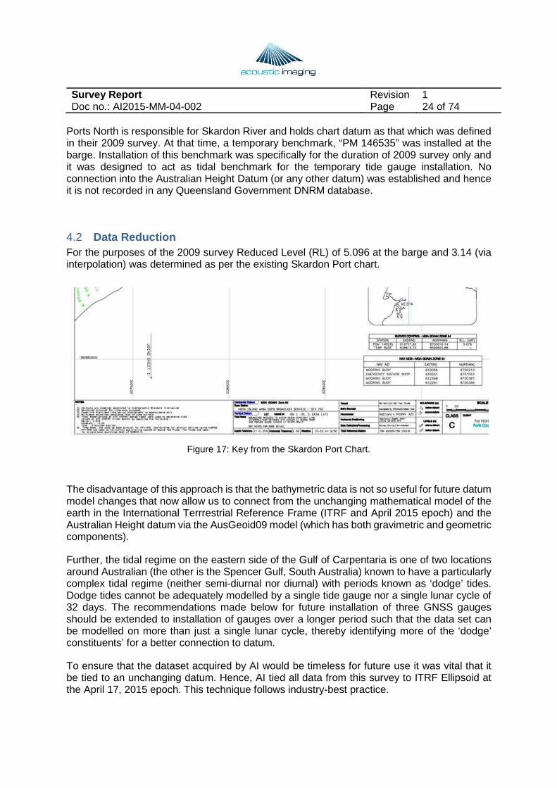
4.2 Data Reduction For the purposes of the 2009 survey Reduced Level (RL) of 5.096 at the barge and 3.14 (via interpolation) was determined as per the existing Skardon Port chart.
Figure 17: Key from the Skardon Port Chart.
The disadvantage of this approach is that the bathymetric data is not so useful for future datum model changes that now allow us to connect from the unchanging mathematical model of the earth in the International Terrrestrial Reference Frame (ITRF and April 2015 epoch) and the Australian Height datum via the AusGeoid09 model (which has both gravimetric and geometric components).
Further, the tidal regime on the eastern side of the Gulf of Carpentaria is one of two locations around Australian (the other is the Spencer Gulf, South Australia) known to have a particularly complex tidal regime (neither semi-diurnal nor diurnal) with periods known as ‘dodge’ tides. Dodge tides cannot be adequately modelled by a single tide gauge nor a single lunar cycle of 32 days. The recommendations made below for future installation of three GNSS gauges should be extended to installation of gauges over a longer period such that the data set can be modelled on more than just a single lunar cycle, thereby identifying more of the ‘dodge’ constituents’ for a better connection to datum.
To ensure that the dataset acquired by AI would be timeless for future use it was vital that it be tied to an unchanging datum. Hence, AI tied all data from this survey to ITRF Ellipsoid at the April 17, 2015 epoch. This technique follows industry-best practice.
Survey Report Revision 1 Doc no.: AI2015-MM-04-002 Page 25 of 74
From the ITRF Ellipsoid we reduced the data set to the Australian Height Datum, and finally to the MSQ-defined LAT in 2009 by empirical analysis.
We used a three-step procedure for connecting the horizontal and vertical positioning to a relevant datum.
In the first step the positioning and orientation data were logged and then post-processed with precise ephemeris and atomic clock correction data to achieve a sub-10cm vertical and horizontal accuracy.
The second step required transformation of the ITRF referenced dataset to GDA94 at the epoch of 17 May 2015 using the coordinates established in Section 2 of the document. These parameters were independently checked for accuracy in two different data transformation software packages.
The third reduction step employed Australia’s national vertical geoid model (AUSGEOID09). This model reduced the dataset from the GDA94 vertical height to the Australian Height Datum (AHD). It was thus rendered compatible with existing surrounding LIDAR data which was reduced through implementation of the same model.
The final empirically-derived LAT reduction of the gridded data is described in the Data Processing section of this report.
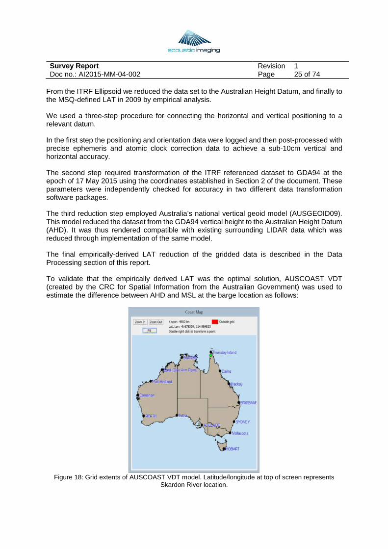
To validate that the empirically derived LAT was the optimal solution, AUSCOAST VDT (created by the CRC for Spatial Information from the Australian Government) was used to estimate the difference between AHD and MSL at the barge location as follows:
Figure 18: Grid extents of AUSCOAST VDT model. Latitude/longitude at top of screen represents Skardon River location.
Survey Report Revision 1 Doc no.: AI2015-MM-04-002 Page 26 of 74
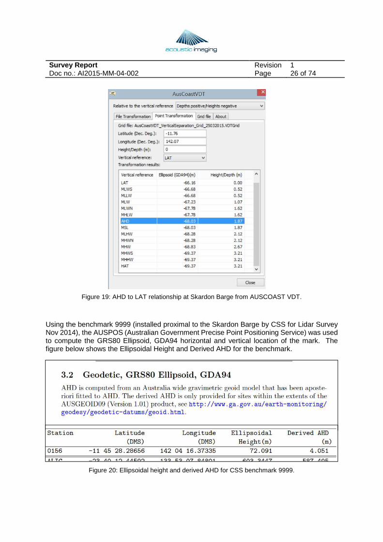
Figure 19: AHD to LAT relationship at Skardon Barge from AUSCOAST VDT.
Using the benchmark 9999 (installed proximal to the Skardon Barge by CSS for Lidar Survey Nov 2014), the AUSPOS (Australian Government Precise Point Positioning Service) was used to compute the GRS80 Ellipsoid, GDA94 horizontal and vertical location of the mark. The figure below shows the Ellipsoidal Height and Derived AHD for the benchmark.
Figure 20: Ellipsoidal height and derived AHD for CSS benchmark 9999.
Survey Report Revision 1 Doc no.: AI2015-MM-04-002 Page 27 of 74
From this result the Ellipsoid to AHD separation at the mark is 68.04 (72.091-4.051).
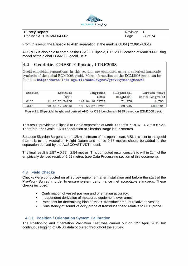
AUSPOS is also able to compute the GRS80 Ellipsoid, ITRF2008 location of Mark 9999 using model of the global EGM2008 geoid. It is:
Figure 21: Ellipsoidal height and derived AHD for CSS benchmark 9999 based on EGM2008 geoid.
This result provides a Ellipsoid to Geoid separation at Mark 9999 of = 71.976 – 4.706 = 67.27. Therefore, the Geoid – AHD separation at Skardon Barge is 0.77metres.
Because Skardon Barge is some 12km upstream of the open ocean, MSL is closer to the geoid than it is to the Australian Height Datum and hence 0.77 metres should be added to the separation derived by the AUSCOAST VDT model.
The final result is 1.87 + 0.77 = 2.54 metres, This computed result concurs to within 2cm of the empirically derived result of 2.52 metres (see Data Processing section of this document).
4.3 Field Checks Checks were conducted on all survey equipment after installation and before the start of the Pre-Work Survey in order to ensure system performance met acceptable standards. These checks included:
• Confirmation of vessel position and orientation accuracy; • Independent derivation of measured equipment lever arms; • Patch test for determining bias of MBES transducer mount relative to vessel; • Consistency of sound velocity probe at transducer head relative to CTD probe.
4.3.1 Position / Orientation System Calibration The Positioning and Orientation Validation Test was carried out on 12th April, 2015 but continuous logging of GNSS data occurred throughout the survey.

Survey Report Revision 1 Doc no.: AI2015-MM-04-002 Page 28 of 74
Accuracy estimates for the real-time data were displayed in the POSView software and monitored during acquisition operations. However, we conducted further validation checks with the logged data during post-processing.
The first of the position and orientation field checks conducted was the GNSS Azimuth Measurement Subsystem (GAMS) heading calibration.
For the calibration, the vessel navigated a series of tight “figure of 8” turns. With each successive turn, the vector between the primary and secondary antenna increases in accuracy. When the accuracy was less than 0.02 degrees, that vector was considered calibrated. The figure below shows the results for the X, Y, and Z vectors.
Figure 22: GAMS baseline vector calibration results for Dolphin installation.
Three iterations of the GAMS baseline vector calibration test were conducted, with each result deviating by no more than 2mm.

Survey Report Revision 1 Doc no.: AI2015-MM-04-002 Page 29 of 74
The calibration was further validated in post-processing where the X,Y, and Z vectors converged quickly and accurately as shown in the figure below.
Figure 23: Convergence of X, Y, and Z lever arm vectors in POSPac.
The image part with relationship ID rId42 was not found in the file.
The image part with relationship ID rId42 was not found in the file.
The image part with relationship ID rId42 was not found in the file.
Survey Report Revision 1 Doc no.: AI2015-MM-04-002 Page 30 of 74
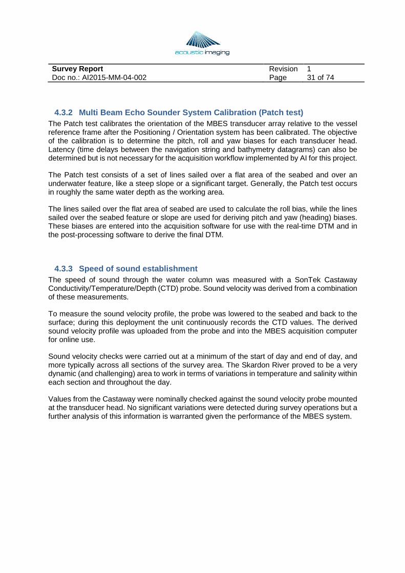
The second part of the Positioning System Calibration is the offset between the IMU to Primary GNSS antenna in the X (fore-aft), Y(port-starboard), and Z (up-down) directions.
Initial offset measurements were done with a tape measure. Vessel data were then logged from Weipa to Skardon River, and this dataset was used in POSPac to calibrate the lever arm measurements. The convergence results are shown in the figure below.
Figure 24: Convergence of lever arms in POSPac.
The figure below shows the final lever arms registered in POSView for acquisition operations.
Figure 25: Final lever arms derived for the IMU to Primary GNSS antenna offset.
The image part with relationship ID rId42 was not found in the file.
The image part with relationship ID rId42 was not found in the file.
The image part with relationship ID rId42 was not found in the file.
Survey Report Revision 1 Doc no.: AI2015-MM-04-002 Page 31 of 74
4.3.2 Multi Beam Echo Sounder System Calibration (P atch test) The Patch test calibrates the orientation of the MBES transducer array relative to the vessel reference frame after the Positioning / Orientation system has been calibrated. The objective of the calibration is to determine the pitch, roll and yaw biases for each transducer head. Latency (time delays between the navigation string and bathymetry datagrams) can also be determined but is not necessary for the acquisition workflow implemented by AI for this project.
The Patch test consists of a set of lines sailed over a flat area of the seabed and over an underwater feature, like a steep slope or a significant target. Generally, the Patch test occurs in roughly the same water depth as the working area.
The lines sailed over the flat area of seabed are used to calculate the roll bias, while the lines sailed over the seabed feature or slope are used for deriving pitch and yaw (heading) biases. These biases are entered into the acquisition software for use with the real-time DTM and in the post-processing software to derive the final DTM.
4.3.3 Speed of sound establishment The speed of sound through the water column was measured with a SonTek Castaway Conductivity/Temperature/Depth (CTD) probe. Sound velocity was derived from a combination of these measurements.
To measure the sound velocity profile, the probe was lowered to the seabed and back to the surface; during this deployment the unit continuously records the CTD values. The derived sound velocity profile was uploaded from the probe and into the MBES acquisition computer for online use.
Sound velocity checks were carried out at a minimum of the start of day and end of day, and more typically across all sections of the survey area. The Skardon River proved to be a very dynamic (and challenging) area to work in terms of variations in temperature and salinity within each section and throughout the day.
Values from the Castaway were nominally checked against the sound velocity probe mounted at the transducer head. No significant variations were detected during survey operations but a further analysis of this information is warranted given the performance of the MBES system.
Survey Report Revision 1 Doc no.: AI2015-MM-04-002 Page 32 of 74
5 Acquisition and Processing
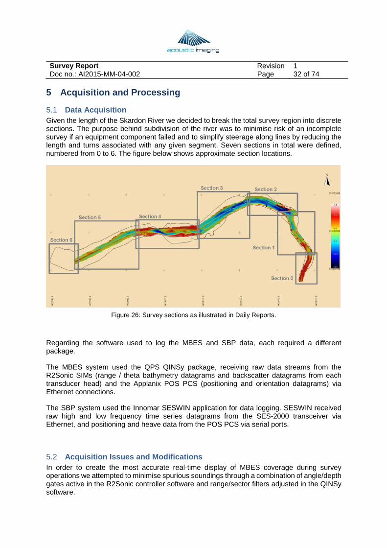
5.1 Data Acquisition Given the length of the Skardon River we decided to break the total survey region into discrete sections. The purpose behind subdivision of the river was to minimise risk of an incomplete survey if an equipment component failed and to simplify steerage along lines by reducing the length and turns associated with any given segment. Seven sections in total were defined, numbered from 0 to 6. The figure below shows approximate section locations.
Figure 26: Survey sections as illustrated in Daily Reports.
Regarding the software used to log the MBES and SBP data, each required a different package.
The MBES system used the QPS QINSy package, receiving raw data streams from the R2Sonic SIMs (range / theta bathymetry datagrams and backscatter datagrams from each transducer head) and the Applanix POS PCS (positioning and orientation datagrams) via Ethernet connections.
The SBP system used the Innomar SESWIN application for data logging. SESWIN received raw high and low frequency time series datagrams from the SES-2000 transceiver via Ethernet, and positioning and heave data from the POS PCS via serial ports.
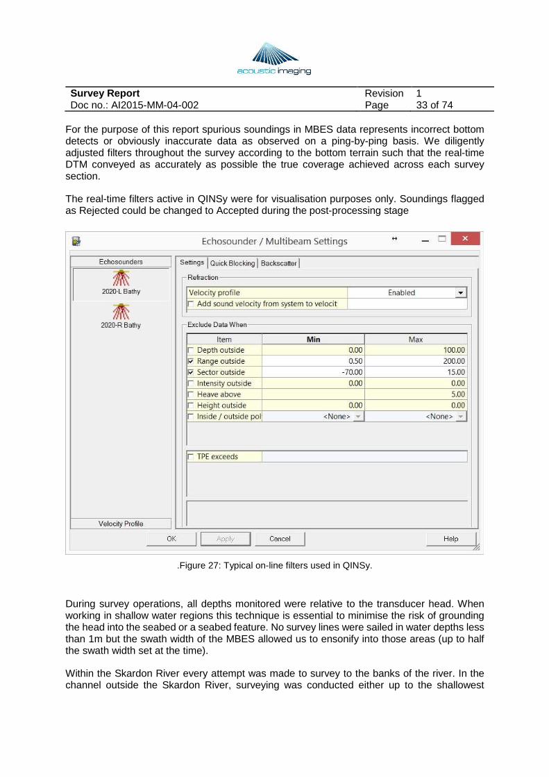
5.2 Acquisition Issues and Modifications In order to create the most accurate real-time display of MBES coverage during survey operations we attempted to minimise spurious soundings through a combination of angle/depth gates active in the R2Sonic controller software and range/sector filters adjusted in the QINSy software.
Survey Report Revision 1 Doc no.: AI2015-MM-04-002 Page 33 of 74
For the purpose of this report spurious soundings in MBES data represents incorrect bottom detects or obviously inaccurate data as observed on a ping-by-ping basis. We diligently adjusted filters throughout the survey according to the bottom terrain such that the real-time DTM conveyed as accurately as possible the true coverage achieved across each survey section.
The real-time filters active in QINSy were for visualisation purposes only. Soundings flagged as Rejected could be changed to Accepted during the post-processing stage
.Figure 27: Typical on-line filters used in QINSy.
During survey operations, all depths monitored were relative to the transducer head. When working in shallow water regions this technique is essential to minimise the risk of grounding the head into the seabed or a seabed feature. No survey lines were sailed in water depths less than 1m but the swath width of the MBES allowed us to ensonify into those areas (up to half the swath width set at the time).
Within the Skardon River every attempt was made to survey to the banks of the river. In the channel outside the Skardon River, surveying was conducted either up to the shallowest
Survey Report Revision 1 Doc no.: AI2015-MM-04-002 Page 34 of 74
sections of bounding sand banks or up to the limits of sand waves affecting safe navigation of the survey vessel.
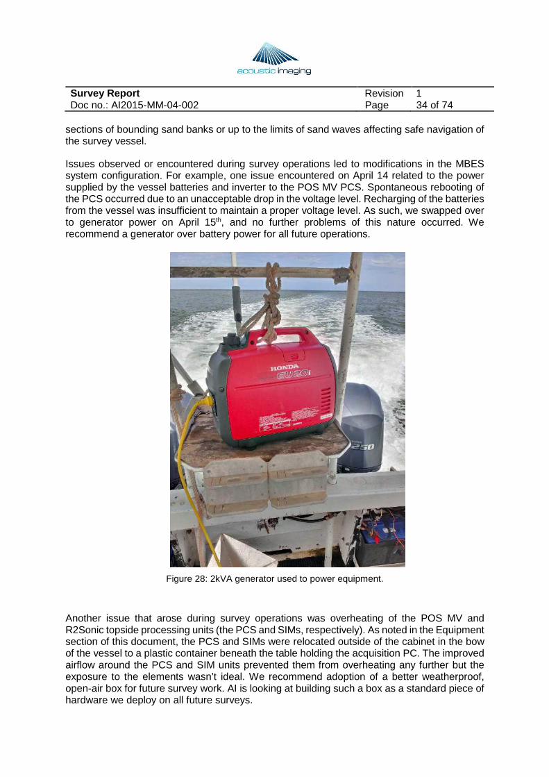
Issues observed or encountered during survey operations led to modifications in the MBES system configuration. For example, one issue encountered on April 14 related to the power supplied by the vessel batteries and inverter to the POS MV PCS. Spontaneous rebooting of the PCS occurred due to an unacceptable drop in the voltage level. Recharging of the batteries from the vessel was insufficient to maintain a proper voltage level. As such, we swapped over to generator power on April 15th, and no further problems of this nature occurred. We recommend a generator over battery power for all future operations.
Figure 28: 2kVA generator used to power equipment.
Another issue that arose during survey operations was overheating of the POS MV and R2Sonic topside processing units (the PCS and SIMs, respectively). As noted in the Equipment section of this document, the PCS and SIMs were relocated outside of the cabinet in the bow of the vessel to a plastic container beneath the table holding the acquisition PC. The improved airflow around the PCS and SIM units prevented them from overheating any further but the exposure to the elements wasn’t ideal. We recommend adoption of a better weatherproof, open-air box for future survey work. AI is looking at building such a box as a standard piece of hardware we deploy on all future surveys.
Survey Report Revision 1 Doc no.: AI2015-MM-04-002 Page 35 of 74
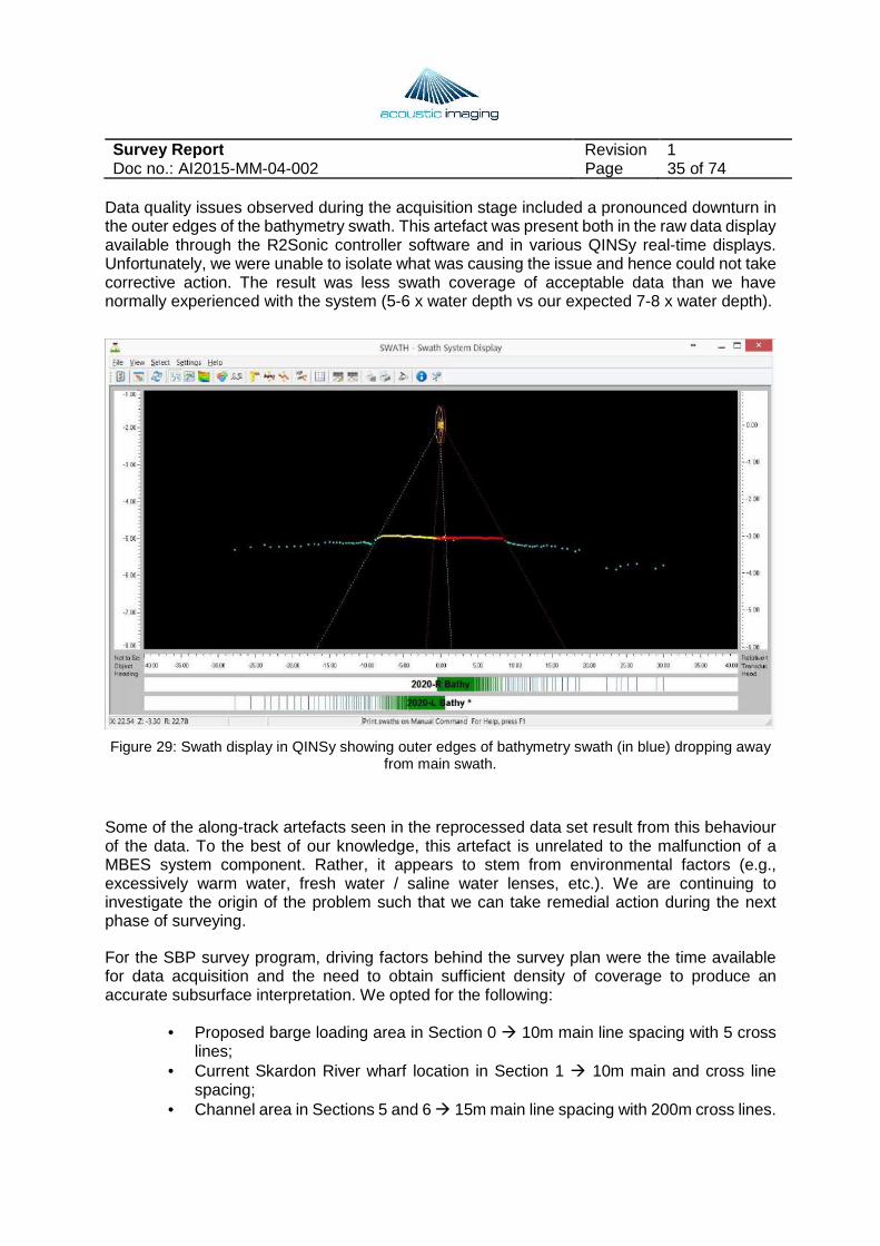
Data quality issues observed during the acquisition stage included a pronounced downturn in the outer edges of the bathymetry swath. This artefact was present both in the raw data display available through the R2Sonic controller software and in various QINSy real-time displays. Unfortunately, we were unable to isolate what was causing the issue and hence could not take corrective action. The result was less swath coverage of acceptable data than we have normally experienced with the system (5-6 x water depth vs our expected 7-8 x water depth).
Figure 29: Swath display in QINSy showing outer edges of bathymetry swath (in blue) dropping away from main swath.
Some of the along-track artefacts seen in the reprocessed data set result from this behaviour of the data. To the best of our knowledge, this artefact is unrelated to the malfunction of a MBES system component. Rather, it appears to stem from environmental factors (e.g., excessively warm water, fresh water / saline water lenses, etc.). We are continuing to investigate the origin of the problem such that we can take remedial action during the next phase of surveying.
For the SBP survey program, driving factors behind the survey plan were the time available for data acquisition and the need to obtain sufficient density of coverage to produce an accurate subsurface interpretation. We opted for the following:
• Proposed barge loading area in Section 0 � 10m main line spacing with 5 cross lines;
• Current Skardon River wharf location in Section 1 � 10m main and cross line spacing;
• Channel area in Sections 5 and 6 � 15m main line spacing with 200m cross lines.
Survey Report Revision 1 Doc no.: AI2015-MM-04-002 Page 36 of 74
As we had no prior experience working in the Skardon River the level of penetration for any given frequency/pulse combination associated with the SBP system was unknown. We conducted some testing in each area prior to running the main survey lines and adjusted the low frequency channel of the Innomar system to best address the penetration requirements for each survey area. In general, either a 5kHz or 6kHz low frequency setting was used for both the Skardon River areas and the channel outside the river.
Similarly, we adjusted the recording length and delay to maximise the penetration capabilities and horizontal resolution across each survey area.
5.3 Survey Reporting For both the MBES and SBP surveys, we maintained Line Logs to capture significant events occurring throughout the course of a day. These records are not included in an Appendix but can be supplied upon request.
Data backups occurred daily to minimise the risk of data loss due to catastrophic hard drive failure.
Daily reports issued to MM captured day-to-day operations and survey progress. These reports are not included as an Appendix to this document but can be supplied upon request.
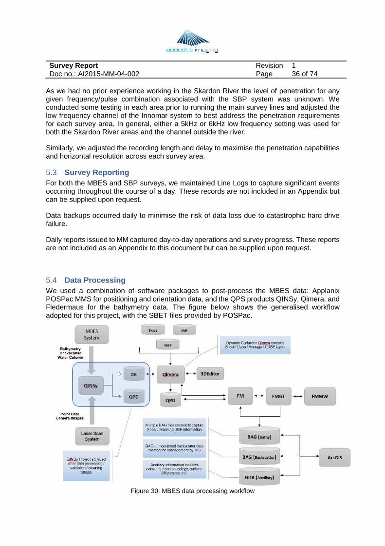
5.4 Data Processing We used a combination of software packages to post-process the MBES data: Applanix POSPac MMS for positioning and orientation data, and the QPS products QINSy, Qimera, and Fledermaus for the bathymetry data. The figure below shows the generalised workflow adopted for this project, with the SBET files provided by POSPac.
Figure 30: MBES data processing workflow
Survey Report Revision 1 Doc no.: AI2015-MM-04-002 Page 37 of 74
The purpose behind reprocessing real-time positioning and orientation data with POSPac MMS is to create a higher accuracy (horizontal and vertical) geospatially-corrected XYZ solution from the raw bathymetry data. We used Qimera to inject the SBET file exported from POSPac into the raw DB files logged by QINSy.
QINSy essentially drops out of the workflow after the acquisition stage. Qimera was used to convert the raw data Range/Theta data stored in the QINSy DB files into a geospatially-corrected solution (QPD format) used for data editing / validation. The products exported from Qimera after editing and validation ranged from a clean sounding set, a gridded sounding set (50cm resolution), and contours.
The Fledermaus Geocoder Toolbox (FMGT) software package was used to process the backscatter data from the MBES. Products exported from FMGT consisted of a backscatter mosaic in GeoTiff format.
Fledermaus (FM) was used for data analysis and interpretation. All data resulting from the survey were loaded into FM as a Scene and viewed relative to one another. The 3D/4D visualisation environment supported by FM helps identify linkages between different data types.
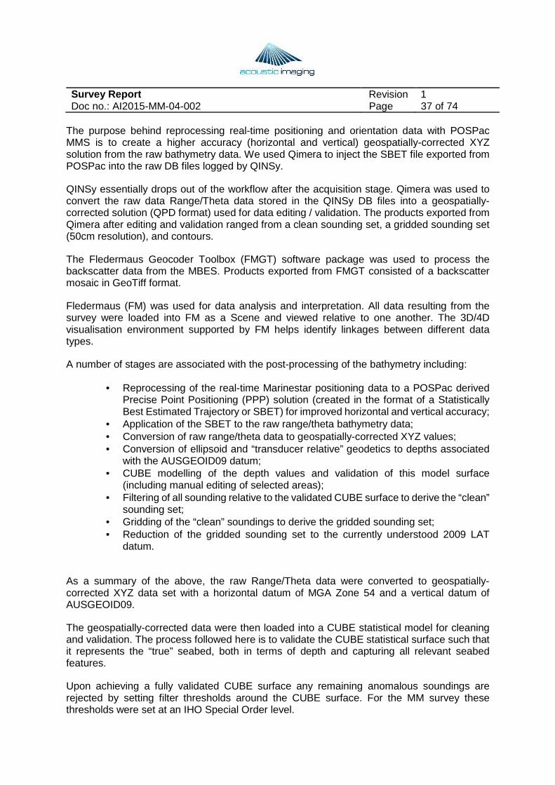
A number of stages are associated with the post-processing of the bathymetry including:
• Reprocessing of the real-time Marinestar positioning data to a POSPac derived Precise Point Positioning (PPP) solution (created in the format of a Statistically Best Estimated Trajectory or SBET) for improved horizontal and vertical accuracy;
• Application of the SBET to the raw range/theta bathymetry data; • Conversion of raw range/theta data to geospatially-corrected XYZ values; • Conversion of ellipsoid and “transducer relative” geodetics to depths associated
with the AUSGEOID09 datum; • CUBE modelling of the depth values and validation of this model surface
(including manual editing of selected areas); • Filtering of all sounding relative to the validated CUBE surface to derive the “clean”
sounding set; • Gridding of the “clean” soundings to derive the gridded sounding set; • Reduction of the gridded sounding set to the currently understood 2009 LAT
datum.
As a summary of the above, the raw Range/Theta data were converted to geospatially-corrected XYZ data set with a horizontal datum of MGA Zone 54 and a vertical datum of AUSGEOID09.
The geospatially-corrected data were then loaded into a CUBE statistical model for cleaning and validation. The process followed here is to validate the CUBE statistical surface such that it represents the “true” seabed, both in terms of depth and capturing all relevant seabed features.
Upon achieving a fully validated CUBE surface any remaining anomalous soundings are rejected by setting filter thresholds around the CUBE surface. For the MM survey these thresholds were set at an IHO Special Order level.
Survey Report Revision 1 Doc no.: AI2015-MM-04-002 Page 38 of 74
After applying the CUBE-based filter a final check was done to ensure no remaining data spikes existed across the survey region. This data set forms the Clean Sounding set, and was provided to MM as a set of ASCII XYZ files. The datum associated with the Clean Sounding set is AHD (AUSGEOID09).
The Clean Sounding set was then gridded at a 0.5m level to create the Gridded Sounding set. The gridding technique used was a Weighted Moving Average with a Weight Diameter parameter of 3.
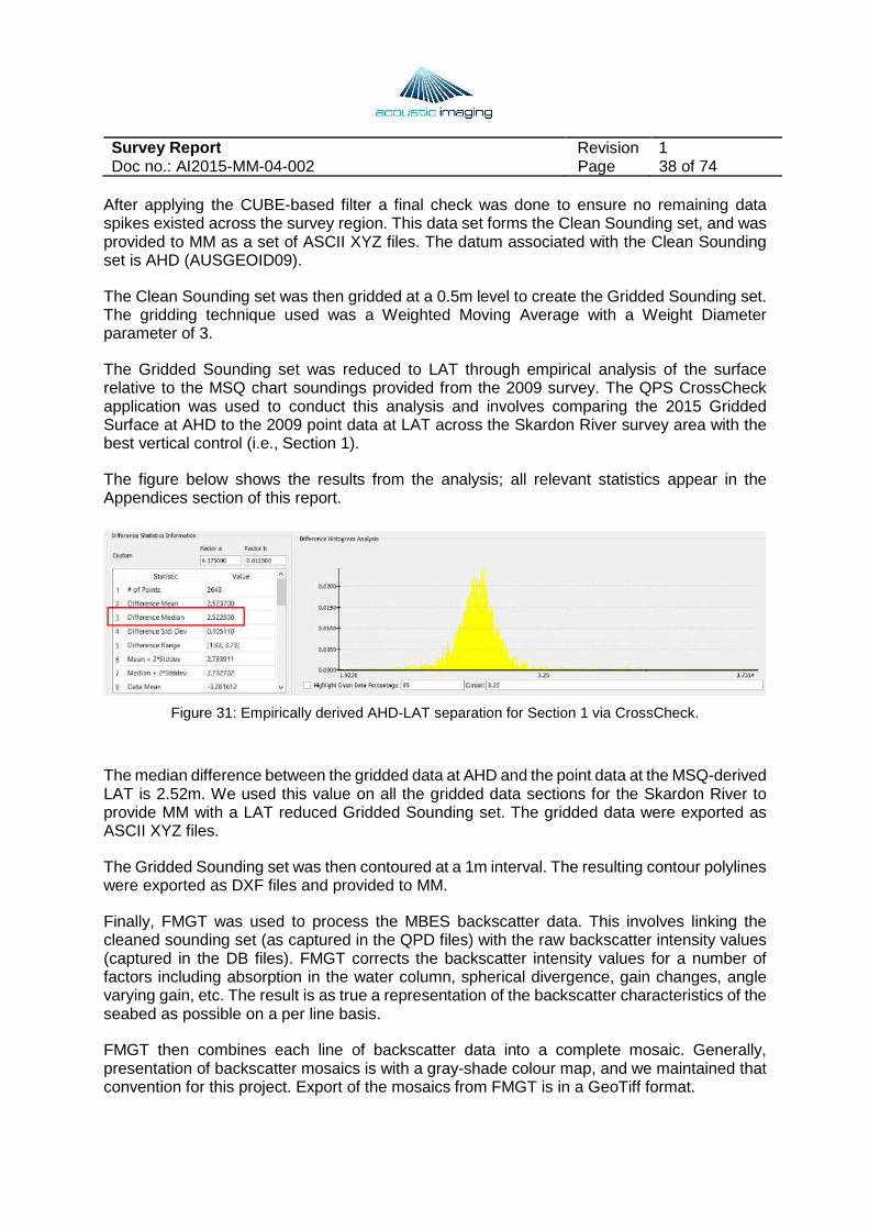
The Gridded Sounding set was reduced to LAT through empirical analysis of the surface relative to the MSQ chart soundings provided from the 2009 survey. The QPS CrossCheck application was used to conduct this analysis and involves comparing the 2015 Gridded Surface at AHD to the 2009 point data at LAT across the Skardon River survey area with the best vertical control (i.e., Section 1).
The figure below shows the results from the analysis; all relevant statistics appear in the Appendices section of this report.
Figure 31: Empirically derived AHD-LAT separation for Section 1 via CrossCheck.
The median difference between the gridded data at AHD and the point data at the MSQ-derived LAT is 2.52m. We used this value on all the gridded data sections for the Skardon River to provide MM with a LAT reduced Gridded Sounding set. The gridded data were exported as ASCII XYZ files.
The Gridded Sounding set was then contoured at a 1m interval. The resulting contour polylines were exported as DXF files and provided to MM.
Finally, FMGT was used to process the MBES backscatter data. This involves linking the cleaned sounding set (as captured in the QPD files) with the raw backscatter intensity values (captured in the DB files). FMGT corrects the backscatter intensity values for a number of factors including absorption in the water column, spherical divergence, gain changes, angle varying gain, etc. The result is as true a representation of the backscatter characteristics of the seabed as possible on a per line basis.
FMGT then combines each line of backscatter data into a complete mosaic. Generally, presentation of backscatter mosaics is with a gray-shade colour map, and we maintained that convention for this project. Export of the mosaics from FMGT is in a GeoTiff format.
Survey Report Revision 1 Doc no.: AI2015-MM-04-002 Page 39 of 74
Post-processing of the SBP data occurred through a combination of the Innomar SESConvert and ISE packages and the Chesapeake Technology SonarWiz package.
SESConvert was used to convert the raw time series data (logged in .SES format) to the non-proprietary SEG-Y format.
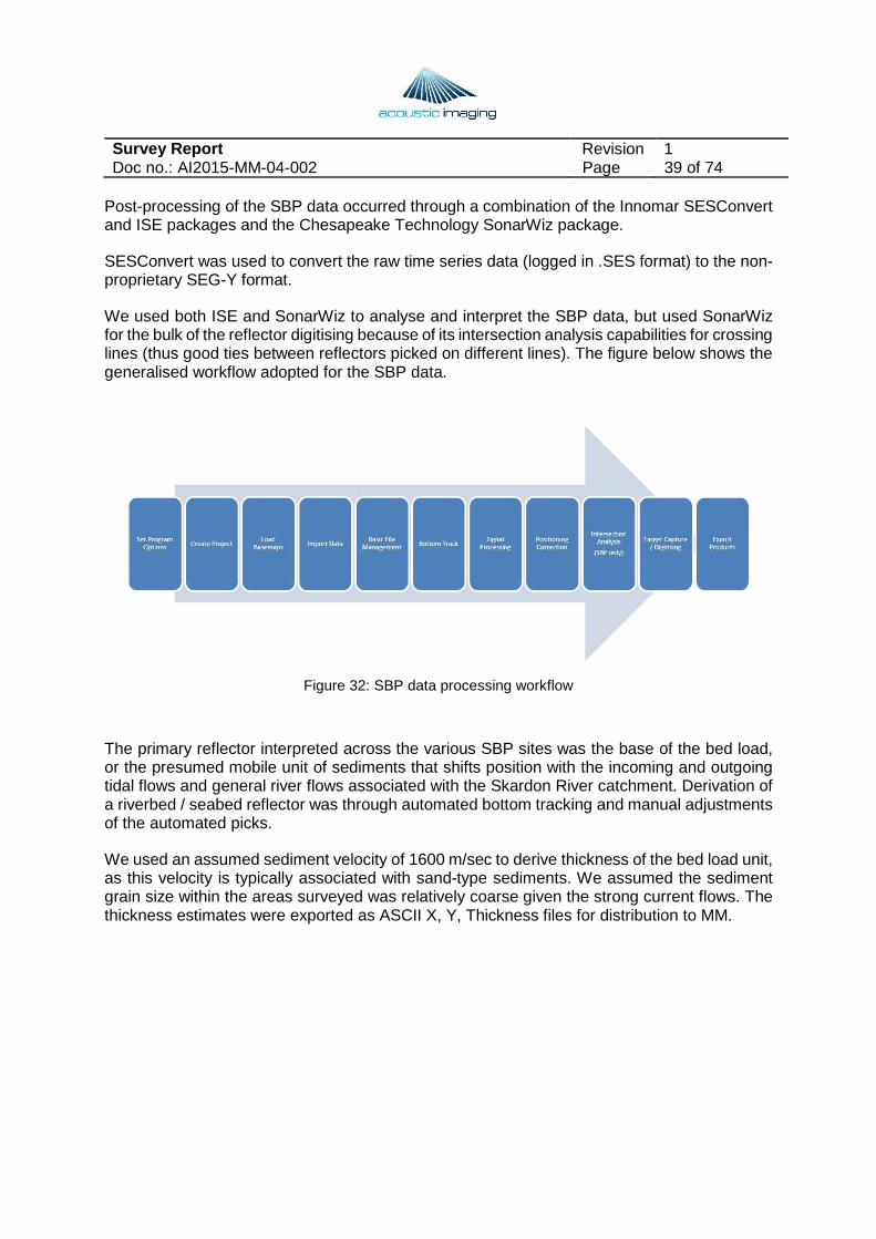
We used both ISE and SonarWiz to analyse and interpret the SBP data, but used SonarWiz for the bulk of the reflector digitising because of its intersection analysis capabilities for crossing lines (thus good ties between reflectors picked on different lines). The figure below shows the generalised workflow adopted for the SBP data.
Figure 32: SBP data processing workflow
The primary reflector interpreted across the various SBP sites was the base of the bed load, or the presumed mobile unit of sediments that shifts position with the incoming and outgoing tidal flows and general river flows associated with the Skardon River catchment. Derivation of a riverbed / seabed reflector was through automated bottom tracking and manual adjustments of the automated picks.
We used an assumed sediment velocity of 1600 m/sec to derive thickness of the bed load unit, as this velocity is typically associated with sand-type sediments. We assumed the sediment grain size within the areas surveyed was relatively coarse given the strong current flows. The thickness estimates were exported as ASCII X, Y, Thickness files for distribution to MM.
Survey Report Revision 1 Doc no.: AI2015-MM-04-002 Page 40 of 74
5.5 Software packages
• The software packages used to acquire and process the data include: • R2Sonic Sonic Controller for real-time control, monitoring, processing, and
filtering of raw bathymetry data arriving from R2Sonic transducers. • Applanix POSView for real-time monitoring and logging of POS MV positioning
and orientation data • Applanix POSPac MMS for post-processing of POS MV positioning and
orientation data • SonTek Castaway software for conversion of raw CTD data to SVP files used in
QINSy • QPS QINSy for MBES data acquisition and real-time processing • QPS Qimera for post-processing of MBES data and data validation / editing • QPS Fledermaus for MBES and SBP data analysis and interpretation • Innomar SESWIN for SBP data acquisition • Innomar SESConvert for conversion of raw SES format files to SEG-Y format • Innomar ISE for selected data analysis • Chesapeake SonarWiz for post-processing, reflector digitising, interpretation, and
unit thickness computations.
Survey Report Revision 1 Doc no.: AI2015-MM-04-002 Page 41 of 74
6 Interpretation and Results The following subsections provide a brief description of seabed and subsurface features across each of the seven survey areas comprising this project. Greater emphasis is placed on Sections 0, 1, 5, and 6 because these areas contain the full suite of geophysical data acquired during the survey and were of most interest to MM.
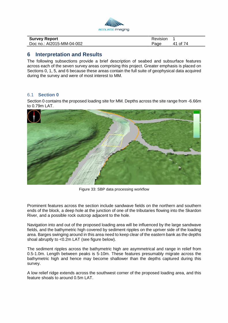
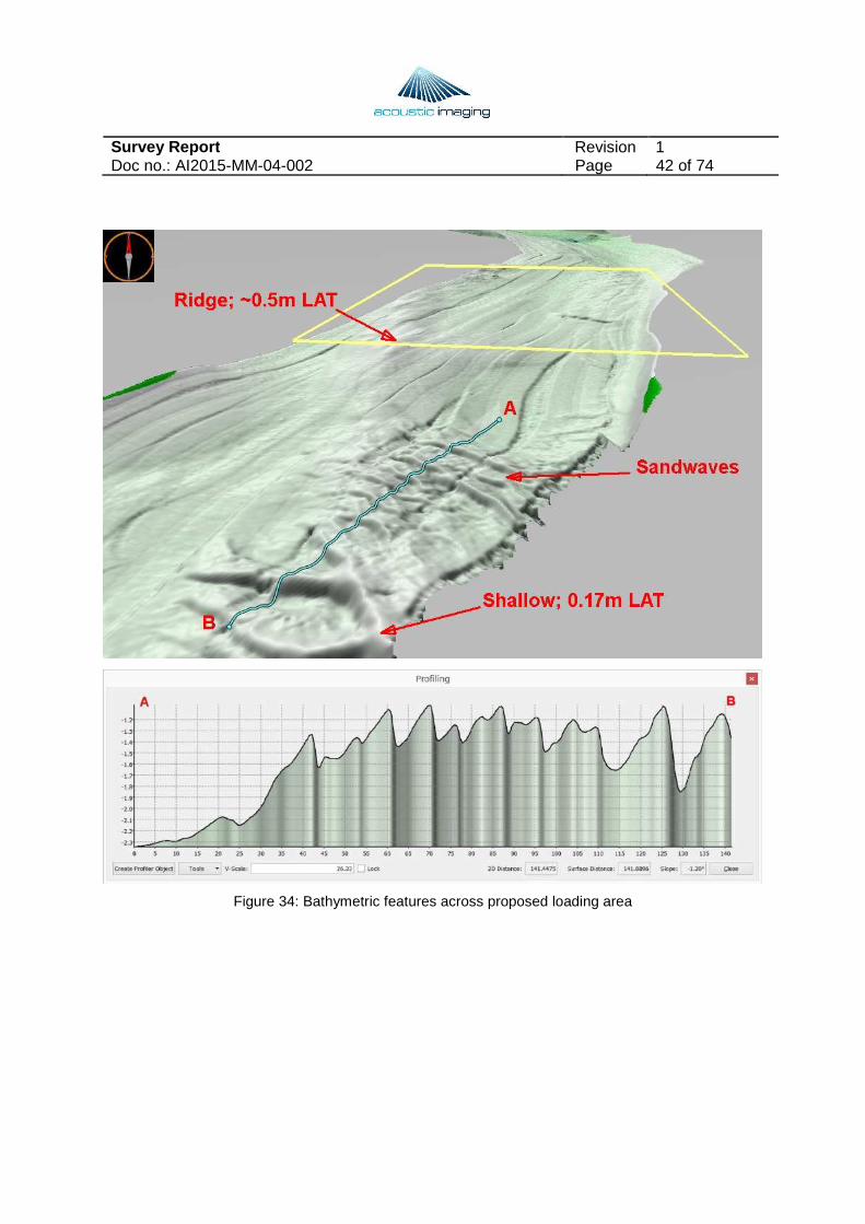
6.1 Section 0 Section 0 contains the proposed loading site for MM. Depths across the site range from -6.66m to 0.79m LAT.
Figure 33: SBP data processing workflow
Prominent features across the section include sandwave fields on the northern and southern ends of the block, a deep hole at the junction of one of the tributaries flowing into the Skardon River, and a possible rock outcrop adjacent to the hole.
Navigation into and out of the proposed loading area will be influenced by the large sandwave fields, and the bathymetric high covered by sediment ripples on the upriver side of the loading area. Barges swinging around in this area need to keep clear of the eastern bank as the depths shoal abruptly to <0.2m LAT (see figure below).
The sediment ripples across the bathymetric high are asymmetrical and range in relief from 0.5-1.0m. Length between peaks is 5-10m. These features presumably migrate across the bathymetric high and hence may become shallower than the depths captured during this survey.
A low relief ridge extends across the southwest corner of the proposed loading area, and this feature shoals to around 0.5m LAT.
Survey Report Revision 1 Doc no.: AI2015-MM-04-002 Page 42 of 74
Figure 34: Bathymetric features across proposed loading area

Survey Report Revision 1 Doc no.: AI2015-MM-04-002 Page 43 of 74
In the SBP data, the bedload thickness varies from less than 1.0m (across the ridge) to >3m in the northeast corner of the proposed loading area.
Figure 35: Bedload thickness across proposed loading area
The figure below shows a representative example of the SBP data across the proposed loading area.
Figure 36: SBP data across proposed loading area
Survey Report Revision 1 Doc no.: AI2015-MM-04-002 Page 44 of 74
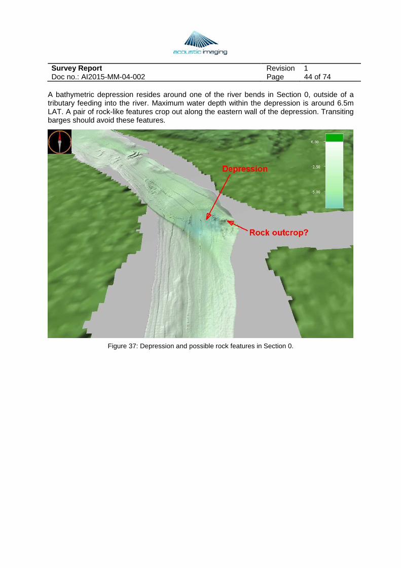
A bathymetric depression resides around one of the river bends in Section 0, outside of a tributary feeding into the river. Maximum water depth within the depression is around 6.5m LAT. A pair of rock-like features crop out along the eastern wall of the depression. Transiting barges should avoid these features.
Figure 37: Depression and possible rock features in Section 0.
Survey Report Revision 1 Doc no.: AI2015-MM-04-002 Page 45 of 74
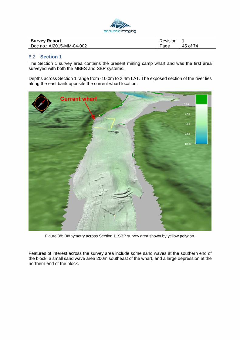
6.2 Section 1 The Section 1 survey area contains the present mining camp wharf and was the first area surveyed with both the MBES and SBP systems.
Depths across Section 1 range from -10.0m to 2.4m LAT. The exposed section of the river lies along the east bank opposite the current wharf location.
Figure 38: Bathymetry across Section 1. SBP survey area shown by yellow polygon.
Features of interest across the survey area include some sand waves at the southern end of the block, a small sand wave area 200m southeast of the whart, and a large depression at the northern end of the block.
Survey Report Revision 1 Doc no.: AI2015-MM-04-002 Page 46 of 74
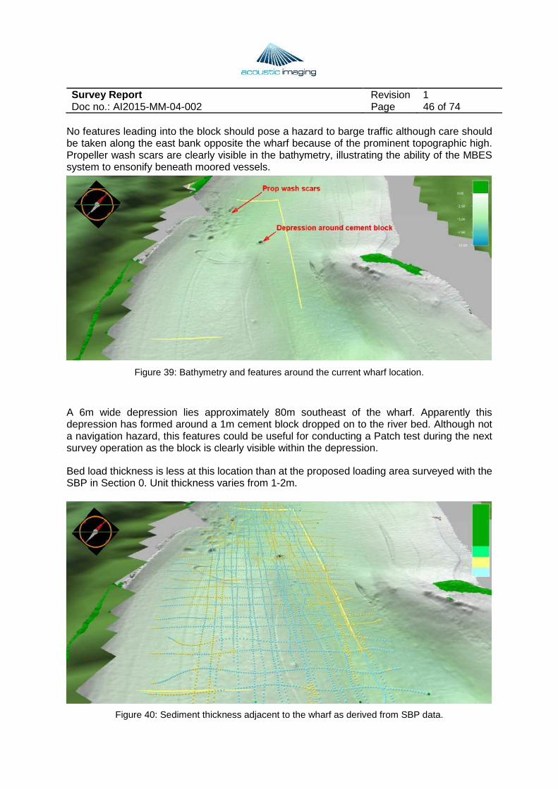
No features leading into the block should pose a hazard to barge traffic although care should be taken along the east bank opposite the wharf because of the prominent topographic high. Propeller wash scars are clearly visible in the bathymetry, illustrating the ability of the MBES system to ensonify beneath moored vessels.
Figure 39: Bathymetry and features around the current wharf location.
A 6m wide depression lies approximately 80m southeast of the wharf. Apparently this depression has formed around a 1m cement block dropped on to the river bed. Although not a navigation hazard, this features could be useful for conducting a Patch test during the next survey operation as the block is clearly visible within the depression.
Bed load thickness is less at this location than at the proposed loading area surveyed with the SBP in Section 0. Unit thickness varies from 1-2m.
Figure 40: Sediment thickness adjacent to the wharf as derived from SBP data.
Survey Report Revision 1 Doc no.: AI2015-MM-04-002 Page 47 of 74
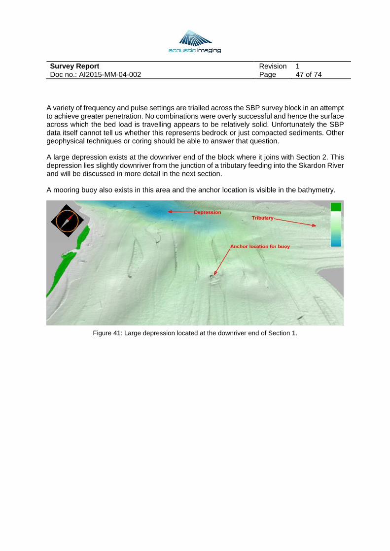
A variety of frequency and pulse settings are trialled across the SBP survey block in an attempt to achieve greater penetration. No combinations were overly successful and hence the surface across which the bed load is travelling appears to be relatively solid. Unfortunately the SBP data itself cannot tell us whether this represents bedrock or just compacted sediments. Other geophysical techniques or coring should be able to answer that question.
A large depression exists at the downriver end of the block where it joins with Section 2. This depression lies slightly downriver from the junction of a tributary feeding into the Skardon River and will be discussed in more detail in the next section.
A mooring buoy also exists in this area and the anchor location is visible in the bathymetry.
Figure 41: Large depression located at the downriver end of Section 1.
Survey Report Revision 1 Doc no.: AI2015-MM-04-002 Page 48 of 74
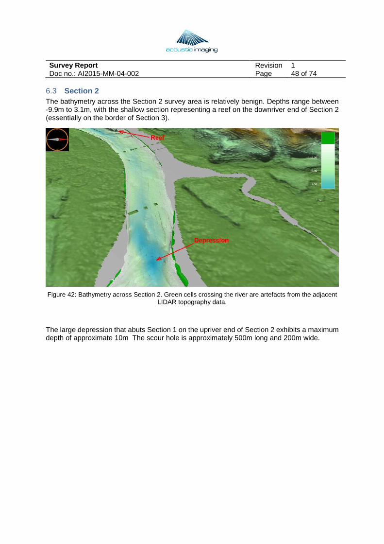
6.3 Section 2 The bathymetry across the Section 2 survey area is relatively benign. Depths range between -9.9m to 3.1m, with the shallow section representing a reef on the downriver end of Section 2 (essentially on the border of Section 3).
Figure 42: Bathymetry across Section 2. Green cells crossing the river are artefacts from the adjacent LIDAR topography data.
The large depression that abuts Section 1 on the upriver end of Section 2 exhibits a maximum depth of approximate 10m The scour hole is approximately 500m long and 200m wide.
Survey Report Revision 1 Doc no.: AI2015-MM-04-002 Page 49 of 74
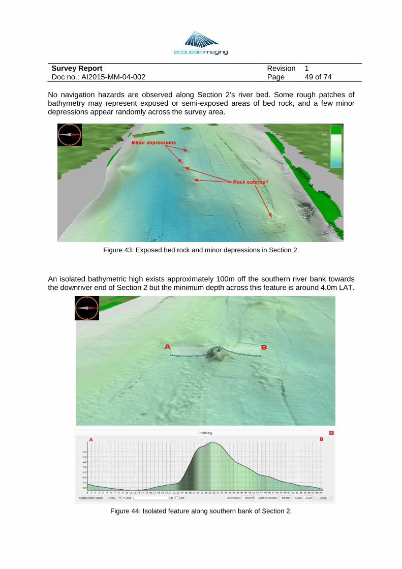
No navigation hazards are observed along Section 2’s river bed. Some rough patches of bathymetry may represent exposed or semi-exposed areas of bed rock, and a few minor depressions appear randomly across the survey area.
Figure 43: Exposed bed rock and minor depressions in Section 2.
An isolated bathymetric high exists approximately 100m off the southern river bank towards the downriver end of Section 2 but the minimum depth across this feature is around 4.0m LAT.
Figure 44: Isolated feature along southern bank of Section 2.
Survey Report Revision 1 Doc no.: AI2015-MM-04-002 Page 50 of 74
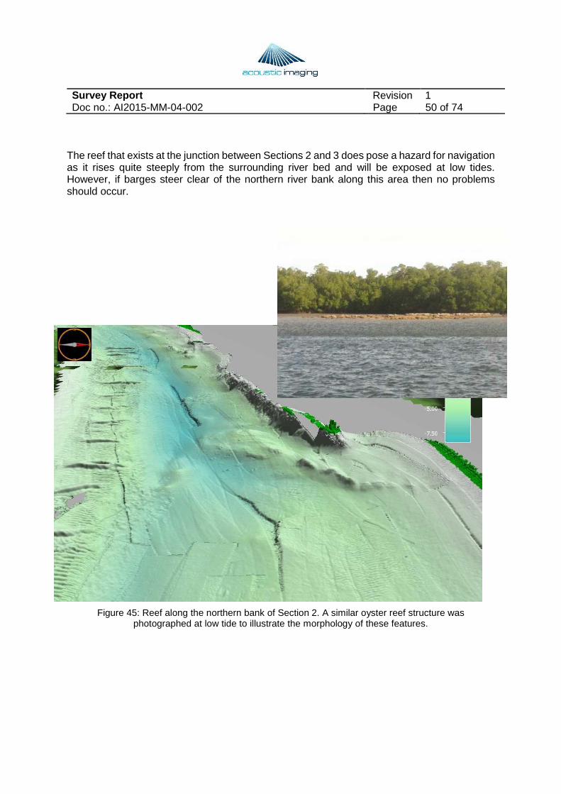
The reef that exists at the junction between Sections 2 and 3 does pose a hazard for navigation as it rises quite steeply from the surrounding river bed and will be exposed at low tides. However, if barges steer clear of the northern river bank along this area then no problems should occur.
Figure 45: Reef along the northern bank of Section 2. A similar oyster reef structure was photographed at low tide to illustrate the morphology of these features.

Survey Report Revision 1 Doc no.: AI2015-MM-04-002 Page 51 of 74
6.4 Section 3 In Section 3 the width of surveyable river section decreases downriver from the reef discussed in Section 2. A large mudflat exists along the northern bank of the river, and safe navigation through this area with the Dolphin was not possible.
Figure 46: Bathymetric and topographic features across Section 3.
Depths across the block range from -8.42m to 2.23m LAT, with the shallow sections appearing along the reef and northern bank in general. The southern bank is quite steep and obstruction-free so it was possible to survey to the edge of the mangroves.
The headland observed in the LIDAR data appears to extend southward towards the reef observed between Sections 2 and 3. As such, the bedrock forming the headland could be the underlying strata beneath oyster reef.
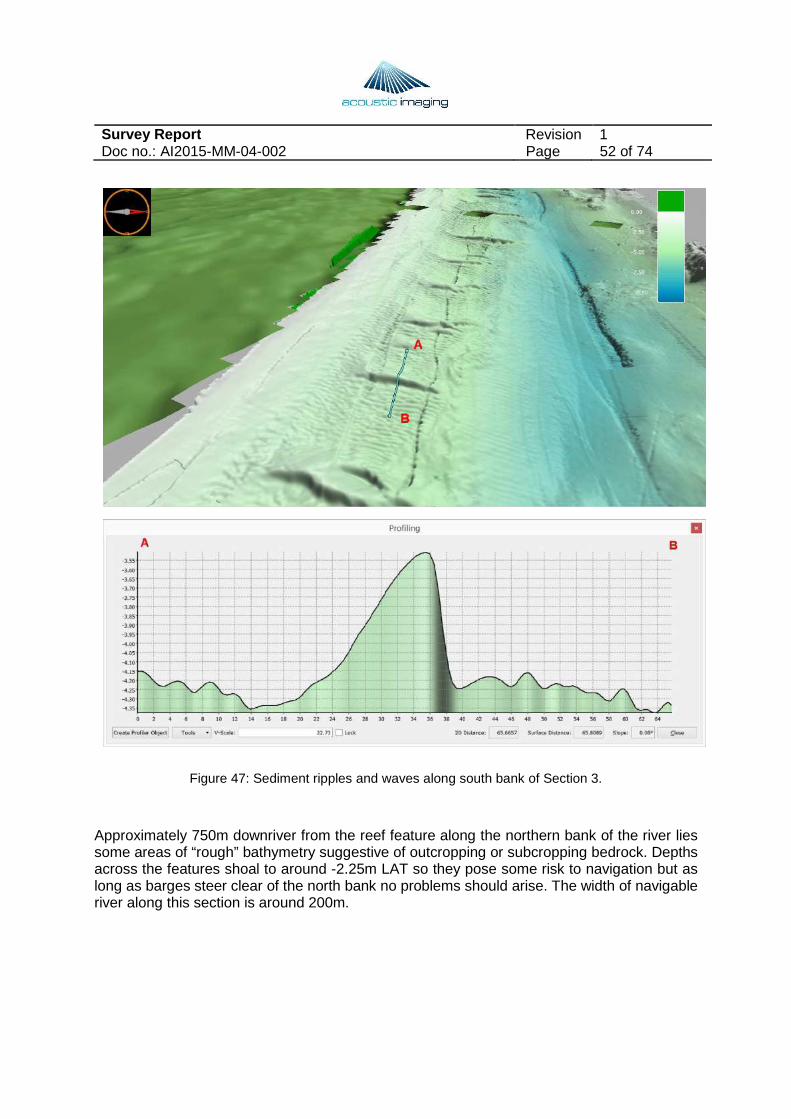
The sediment ripple / wave field along the southern bank indicates a mobile bed load is present but should not represent a hazard to barge navigation. The heights of the ripples are only 0.10-0.15m with the larger waves reaching heights of 0.5-1.0m and lengths of around 20-25m. Water depths across these features do not become shallower than 3.5m LAT but it’s unknown at this time whether these features become more prominent at different stages of river flow.
Survey Report Revision 1 Doc no.: AI2015-MM-04-002 Page 52 of 74
Figure 47: Sediment ripples and waves along south bank of Section 3.
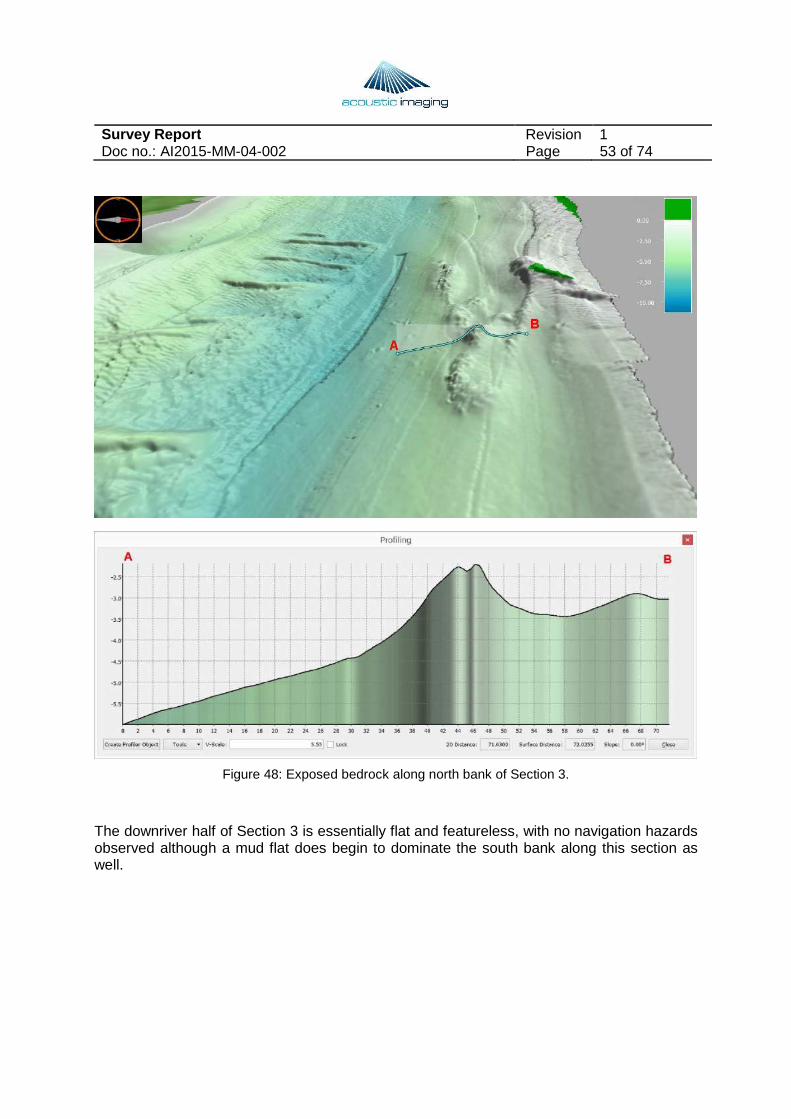
Approximately 750m downriver from the reef feature along the northern bank of the river lies some areas of “rough” bathymetry suggestive of outcropping or subcropping bedrock. Depths across the features shoal to around -2.25m LAT so they pose some risk to navigation but as long as barges steer clear of the north bank no problems should arise. The width of navigable river along this section is around 200m.
Survey Report Revision 1 Doc no.: AI2015-MM-04-002 Page 53 of 74
Figure 48: Exposed bedrock along north bank of Section 3.
The downriver half of Section 3 is essentially flat and featureless, with no navigation hazards observed although a mud flat does begin to dominate the south bank along this section as well.
Survey Report Revision 1 Doc no.: AI2015-MM-04-002 Page 54 of 74
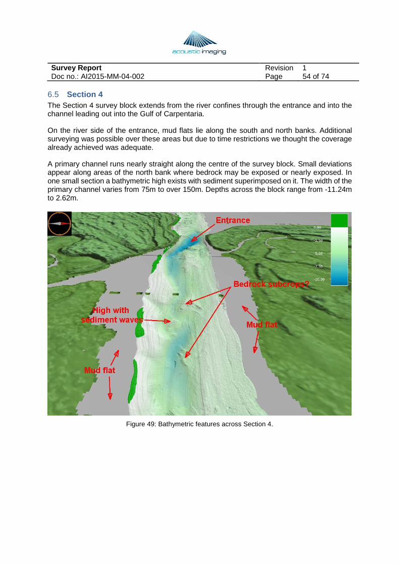
6.5 Section 4 The Section 4 survey block extends from the river confines through the entrance and into the channel leading out into the Gulf of Carpentaria.
On the river side of the entrance, mud flats lie along the south and north banks. Additional surveying was possible over these areas but due to time restrictions we thought the coverage already achieved was adequate.
A primary channel runs nearly straight along the centre of the survey block. Small deviations appear along areas of the north bank where bedrock may be exposed or nearly exposed. In one small section a bathymetric high exists with sediment superimposed on it. The width of the primary channel varies from 75m to over 150m. Depths across the block range from -11.24m to 2.62m.
Figure 49: Bathymetric features across Section 4.
Survey Report Revision 1 Doc no.: AI2015-MM-04-002 Page 55 of 74
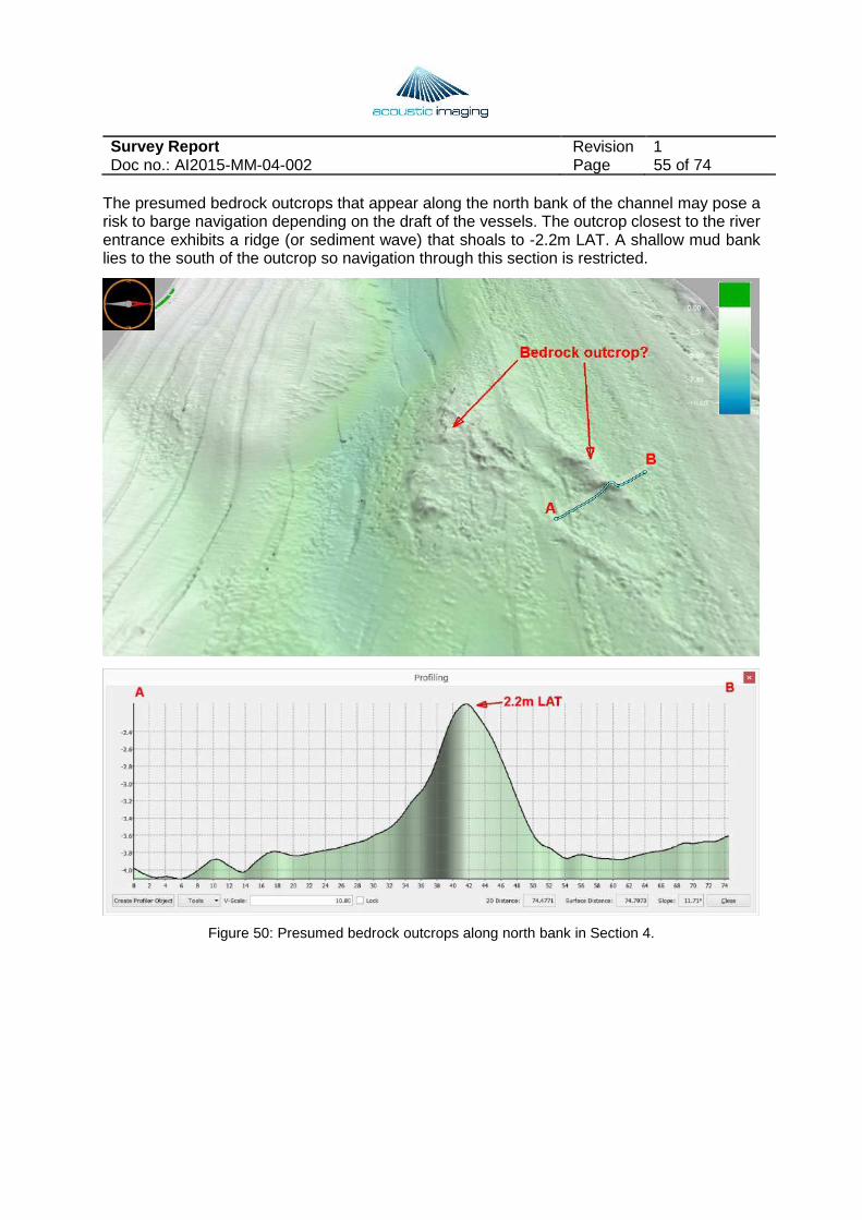
The presumed bedrock outcrops that appear along the north bank of the channel may pose a risk to barge navigation depending on the draft of the vessels. The outcrop closest to the river entrance exhibits a ridge (or sediment wave) that shoals to -2.2m LAT. A shallow mud bank lies to the south of the outcrop so navigation through this section is restricted.
Figure 50: Presumed bedrock outcrops along north bank in Section 4.
Survey Report Revision 1 Doc no.: AI2015-MM-04-002 Page 56 of 74
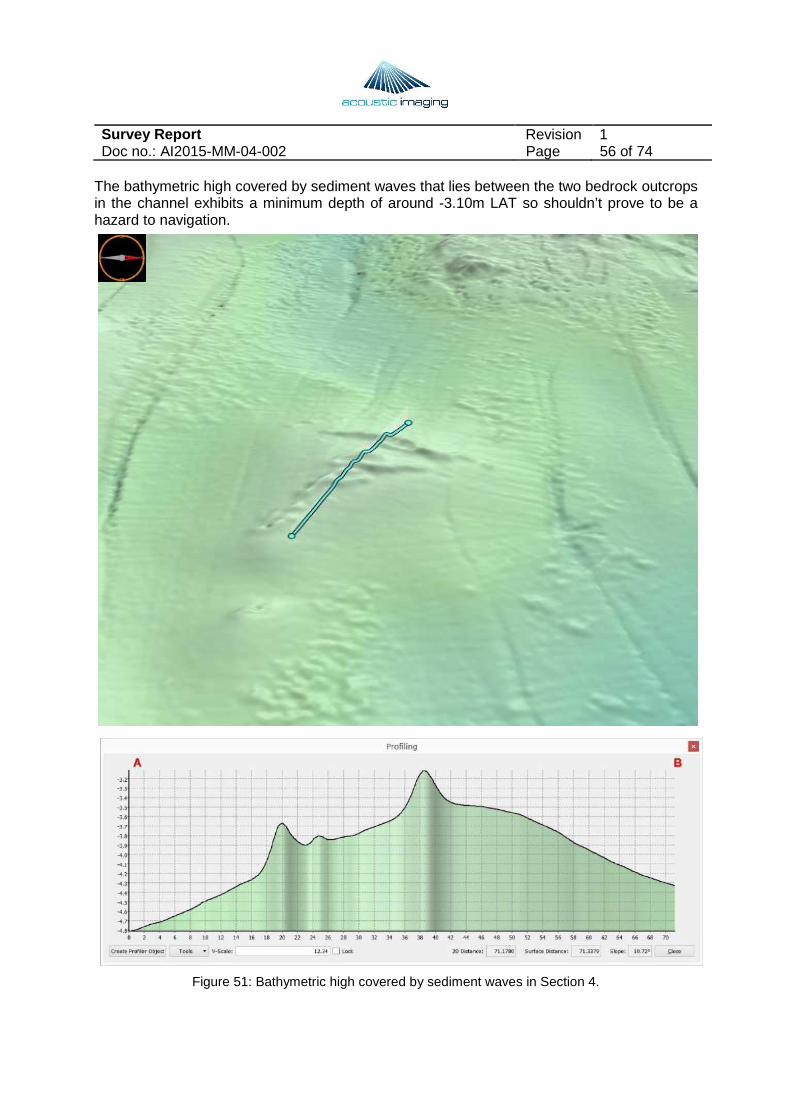
The bathymetric high covered by sediment waves that lies between the two bedrock outcrops in the channel exhibits a minimum depth of around -3.10m LAT so shouldn’t prove to be a hazard to navigation.
Figure 51: Bathymetric high covered by sediment waves in Section 4.
Survey Report Revision 1 Doc no.: AI2015-MM-04-002 Page 57 of 74
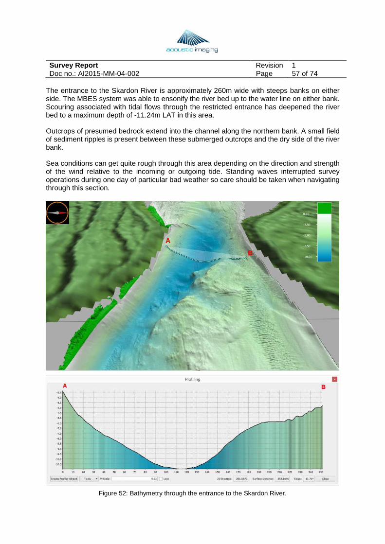
The entrance to the Skardon River is approximately 260m wide with steeps banks on either side. The MBES system was able to ensonify the river bed up to the water line on either bank. Scouring associated with tidal flows through the restricted entrance has deepened the river bed to a maximum depth of -11.24m LAT in this area.
Outcrops of presumed bedrock extend into the channel along the northern bank. A small field of sediment ripples is present between these submerged outcrops and the dry side of the river bank.
Sea conditions can get quite rough through this area depending on the direction and strength of the wind relative to the incoming or outgoing tide. Standing waves interrupted survey operations during one day of particular bad weather so care should be taken when navigating through this section.
Figure 52: Bathymetry through the entrance to the Skardon River.
Survey Report Revision 1 Doc no.: AI2015-MM-04-002 Page 58 of 74
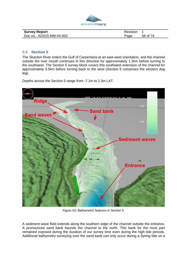
6.6 Section 5 The Skardon River enters the Gulf of Carpentaria at an east-west orientation, and the channel outside the river mouth continues in this direction for approximately 1.2km before turning to the southwest. The Section 5 survey block covers this southwest extension of the channel for approximately 3.5km before turning back to the west (Section 6 comprises the western dog leg).
Depths across the Section 5 range from -7.1m to 2.3m LAT.
Figure 53: Bathymetric features in Section 5.
A sediment wave field extends along the southern edge of the channel outside the entrance. A pronounced sand bank bounds the channel to the north. This bank for the most part remained exposed during the duration of our survey time even during the high tide periods. Additional bathymetry surveying over the sand bank can only occur during a Spring tide on a
Survey Report Revision 1 Doc no.: AI2015-MM-04-002 Page 59 of 74
rising tide. Such conditions did not exist during our April survey so we acquired data where it was safe to navigate.
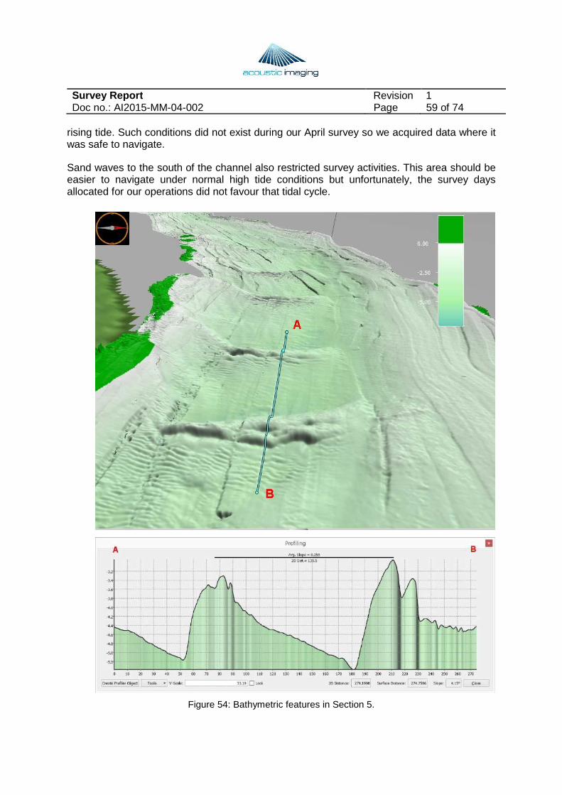
Sand waves to the south of the channel also restricted survey activities. This area should be easier to navigate under normal high tide conditions but unfortunately, the survey days allocated for our operations did not favour that tidal cycle.
Figure 54: Bathymetric features in Section 5.
Survey Report Revision 1 Doc no.: AI2015-MM-04-002 Page 60 of 74
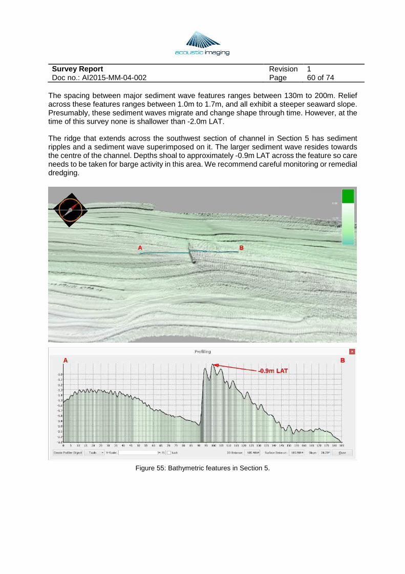
The spacing between major sediment wave features ranges between 130m to 200m. Relief across these features ranges between 1.0m to 1.7m, and all exhibit a steeper seaward slope. Presumably, these sediment waves migrate and change shape through time. However, at the time of this survey none is shallower than -2.0m LAT.
The ridge that extends across the southwest section of channel in Section 5 has sediment ripples and a sediment wave superimposed on it. The larger sediment wave resides towards the centre of the channel. Depths shoal to approximately -0.9m LAT across the feature so care needs to be taken for barge activity in this area. We recommend careful monitoring or remedial dredging.
Figure 55: Bathymetric features in Section 5.
Survey Report Revision 1 Doc no.: AI2015-MM-04-002 Page 61 of 74
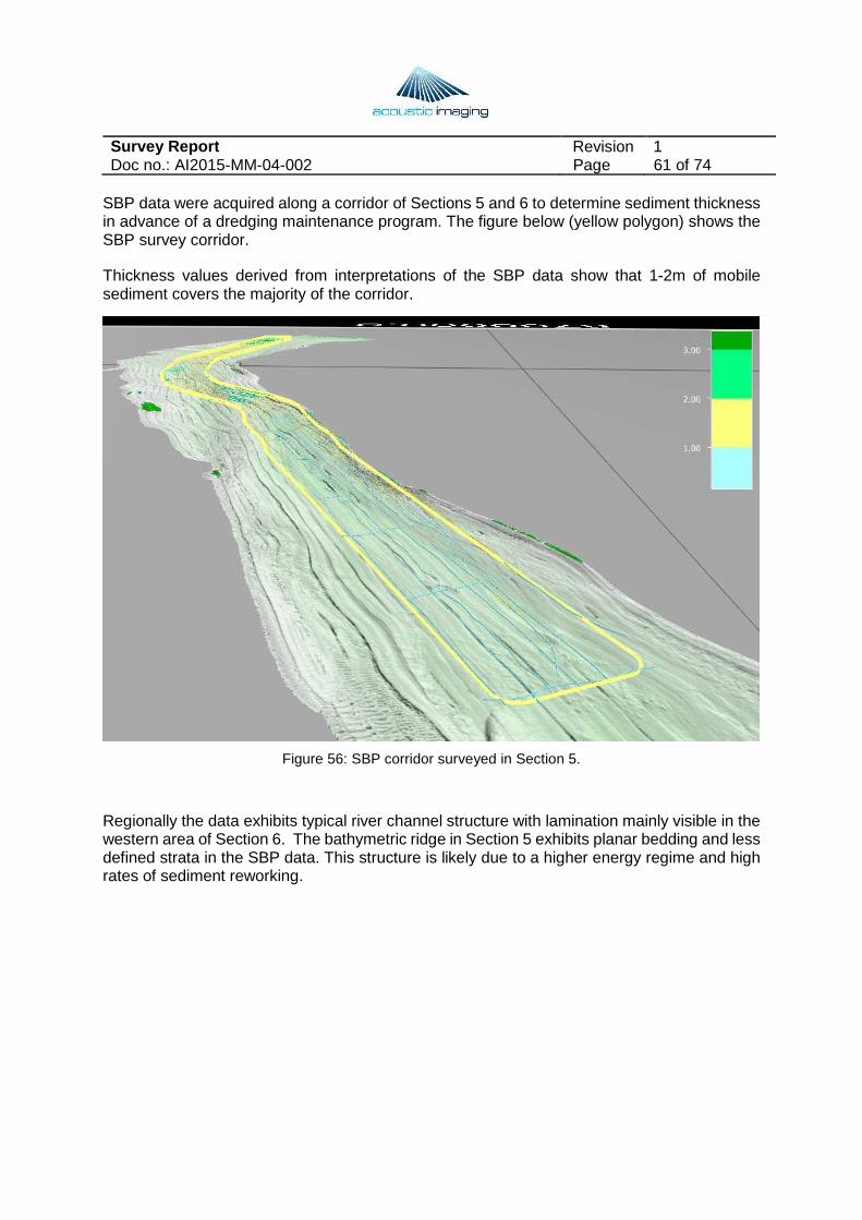
SBP data were acquired along a corridor of Sections 5 and 6 to determine sediment thickness in advance of a dredging maintenance program. The figure below (yellow polygon) shows the SBP survey corridor.
Thickness values derived from interpretations of the SBP data show that 1-2m of mobile sediment covers the majority of the corridor.
Figure 56: SBP corridor surveyed in Section 5.
Regionally the data exhibits typical river channel structure with lamination mainly visible in the western area of Section 6. The bathymetric ridge in Section 5 exhibits planar bedding and less defined strata in the SBP data. This structure is likely due to a higher energy regime and high rates of sediment reworking.
Survey Report Revision 1 Doc no.: AI2015-MM-04-002 Page 62 of 74
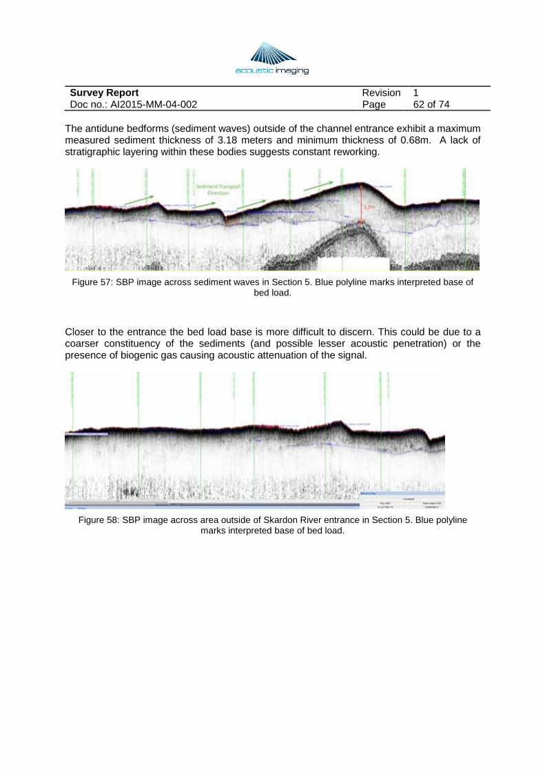
The antidune bedforms (sediment waves) outside of the channel entrance exhibit a maximum measured sediment thickness of 3.18 meters and minimum thickness of 0.68m. A lack of stratigraphic layering within these bodies suggests constant reworking.
Figure 57: SBP image across sediment waves in Section 5. Blue polyline marks interpreted base of bed load.
Closer to the entrance the bed load base is more difficult to discern. This could be due to a coarser constituency of the sediments (and possible lesser acoustic penetration) or the presence of biogenic gas causing acoustic attenuation of the signal.
Figure 58: SBP image across area outside of Skardon River entrance in Section 5. Blue polyline marks interpreted base of bed load.
Survey Report Revision 1 Doc no.: AI2015-MM-04-002 Page 63 of 74
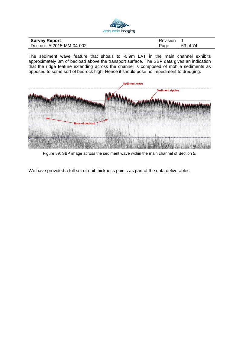
The sediment wave feature that shoals to -0.9m LAT in the main channel exhibits approximately 3m of bedload above the transport surface. The SBP data gives an indication that the ridge feature extending across the channel is composed of mobile sediments as opposed to some sort of bedrock high. Hence it should pose no impediment to dredging.
Figure 59: SBP image across the sediment wave within the main channel of Section 5.
We have provided a full set of unit thickness points as part of the data deliverables.
Survey Report Revision 1 Doc no.: AI2015-MM-04-002 Page 64 of 74
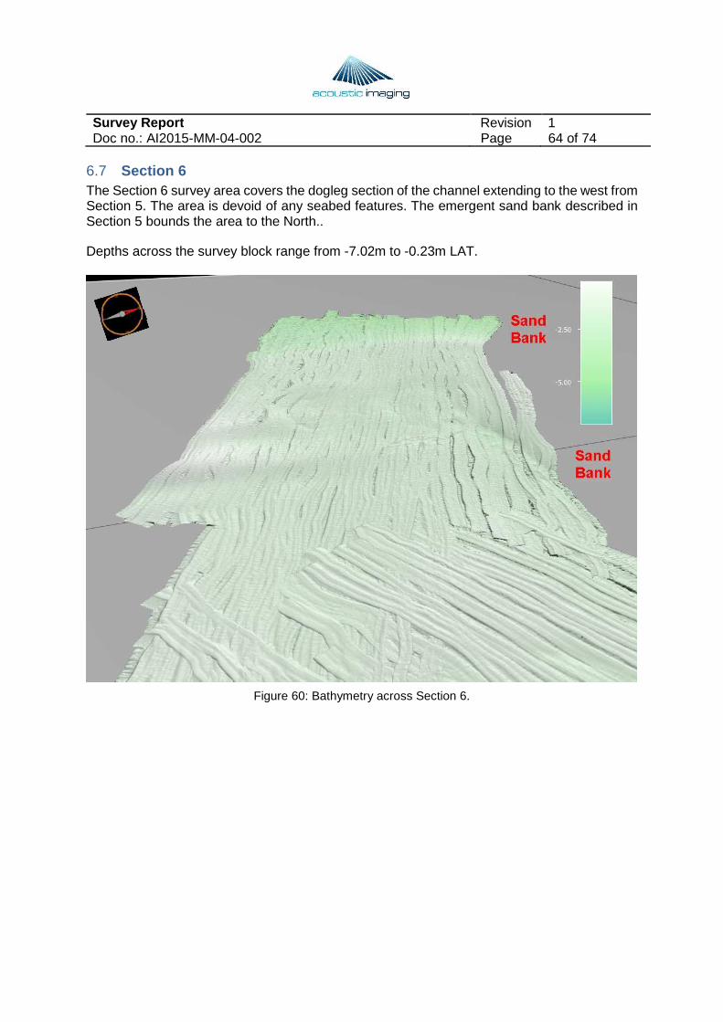
6.7 Section 6 The Section 6 survey area covers the dogleg section of the channel extending to the west from Section 5. The area is devoid of any seabed features. The emergent sand bank described in Section 5 bounds the area to the North..
Depths across the survey block range from -7.02m to -0.23m LAT.
Figure 60: Bathymetry across Section 6.

Survey Report Revision 1 Doc no.: AI2015-MM-04-002 Page 65 of 74
The SBP data across Section 6 show that the bedload thickness ranges between 2-3m.
Figure 61: Bedload thickness derived from SBP data across Section 6.
The SBP data shows a pronounced wedge of sediments across Section 6, presumably extending from the sand bank to the north. Seismic stratigraphic patterns in the profiles show marked cross-bedding dipping westward in the sediment lens. Both the bathymetry and the seismic stratigraphy suggest a prograding sediment lens in a seaward direction.
Figure 62: Stratigraphy associated with sediment lens in Section 6.
Survey Report Revision 1 Doc no.: AI2015-MM-04-002 Page 66 of 74
7 Results and Recommendations The following subsections endeavour to summarise the key results from the entirety of survey operations, and make recommendations for further work in the region.
Our perception of further work in the area is based on:
• Engineering requirements spanning both the land and river environments around the Skardon Barge and proposed barge loading facilities;
• Safe navigation for vessels transiting the river and offshore channel.
7.1 Current Geodetic Control Two primary height data sets exist across the Skardon River area: the land LIDAR data acquired by CSS and the river/channel depth data acquired by AI. Additional river/channel depth data are available from a 2009 survey conducted by MSQ and supplied by Ports North.
Vertical control issues exist between the LIDAR data and the river/channel data, and within the river/channel data set.
The LIDAR data are referenced to a land datum (Australian Height Datum; AHD) and with good vertical control whereas the river/channel data are referenced to a marine datum (nominal Lowest Astronomical Tide; LAT). The nominal LAT value was derived from a temporary tide gauge installed at the Skardon Barge location over a single lunar cycle and relevant to the survey carried out in 2009. No direct tie to AHD was ever established for the temporary tide gauge (and associated temporary benchmark), and no tide gauge network exists within the Skardon River.
The problems to resolve are:
• establishing a direct linkage between AHD and LAT a cross the entirety of the Skardon River, and thus using a common datum fo r all engineering work; and
• establishing a better understanding of the tidal re gime and LAT inside and outside of the Skardon River for navigation safety.
First, let us review the various geodetic levels and linkages associated with these problems.
AUSSGEOID09 (Australia’s national height datum model) connects the Ellipsoid (the reference datum for all GPS/GNSS satellite heights) to AHD.
As noted in the Data Reduction of this document, we logged the raw river/channel data at the Ellipsoid in QINSy. This We then reduced the river/channel data from the Ellipsoid to AUSGEOID09 during the post-processing stage in Qimera. This is the same method used by CSS Lidar survey in Nov 2014. The data was logged to the Ellipsoid then reduced to AHD using AUSGEOI09 model. Although the data were further reduced to LAT in Qimera, our understanding of the accuracy of that datum reduction value for the entire Skardon River area is more tenuous.
Survey Report Revision 1 Doc no.: AI2015-MM-04-002 Page 67 of 74
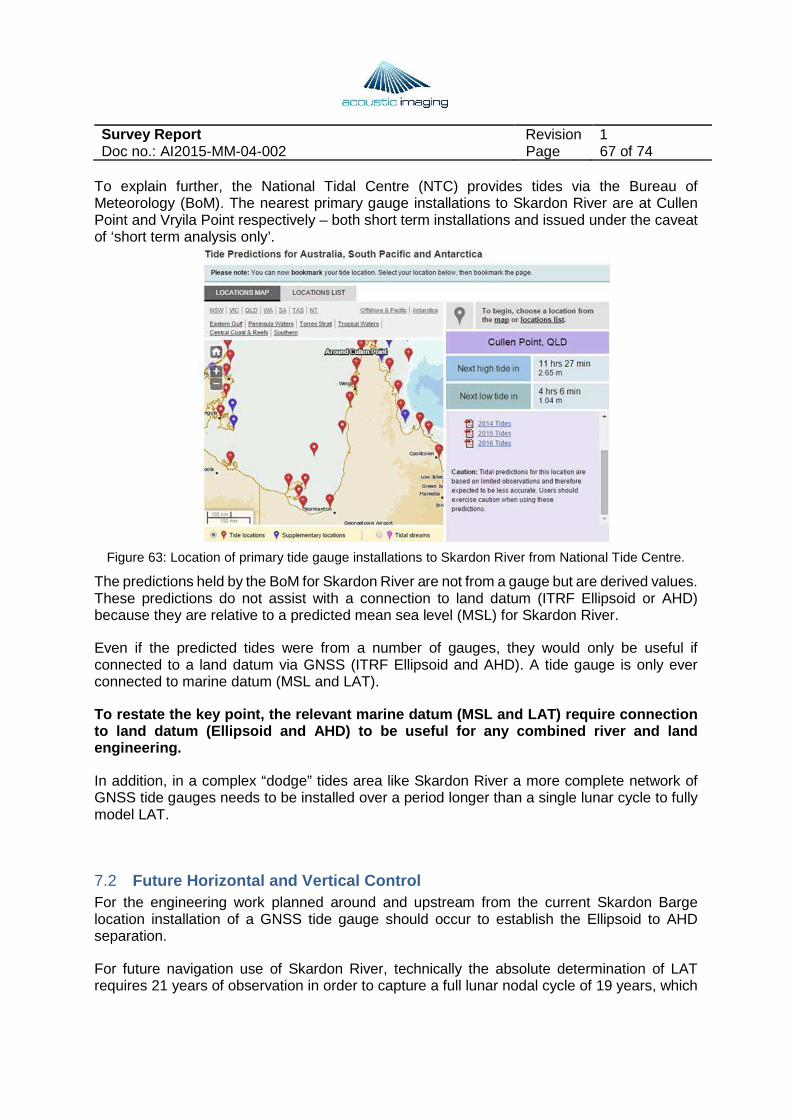
To explain further, the National Tidal Centre (NTC) provides tides via the Bureau of Meteorology (BoM). The nearest primary gauge installations to Skardon River are at Cullen Point and Vryila Point respectively – both short term installations and issued under the caveat of ‘short term analysis only’.
Figure 63: Location of primary tide gauge installations to Skardon River from National Tide Centre.
The predictions held by the BoM for Skardon River are not from a gauge but are derived values. These predictions do not assist with a connection to land datum (ITRF Ellipsoid or AHD) because they are relative to a predicted mean sea level (MSL) for Skardon River.
Even if the predicted tides were from a number of gauges, they would only be useful if connected to a land datum via GNSS (ITRF Ellipsoid and AHD). A tide gauge is only ever connected to marine datum (MSL and LAT).
To restate the key point, the relevant marine datum (MSL and LAT) require connection to land datum (Ellipsoid and AHD) to be useful for any combined river and land engineering.
In addition, in a complex “dodge” tides area like Skardon River a more complete network of GNSS tide gauges needs to be installed over a period longer than a single lunar cycle to fully model LAT.
7.2 Future Horizontal and Vertical Control For the engineering work planned around and upstream from the current Skardon Barge location installation of a GNSS tide gauge should occur to establish the Ellipsoid to AHD separation.
For future navigation use of Skardon River, technically the absolute determination of LAT requires 21 years of observation in order to capture a full lunar nodal cycle of 19 years, which

Survey Report Revision 1 Doc no.: AI2015-MM-04-002 Page 68 of 74
is long enough to average out the local meteorological and oceanographic effects on sea level (and other non-linear coefficients) at a tide gauge.
Where a 20-year observation period is not possible, determination of a relative (or short) tidal datum is acceptable. Relative tidal datum determination requires a logging period of a 30-day full moon cycle.[1] The single full moon cycle is used in comparison with simultaneous observations at an adjacent absolute tidal datum.
In the case of April 2015 Skardon River survey, a full moon cycle was not possible due to the requirement for survey activities to be undertaken immediately and completed as quickly as possible. However, we strongly recommend that if the river is to be used for future navigation purposes that a full analysis of the tidal regime be undertaken. This requires:
• 3 GNSS-receiver enabled gauges; • Locations for tide gauges chosen from upstream infrastructure to mouth of river; • Longer than 32-35 days of gauge deployment (does not require human
intervention except for deployment and recovery) over spring tides for adequate modelling of ‘dodge’ tides.
• Analysis of the gauge data sets and extraction of tidal coefficients for comparison with adjacent gauges at Humbug Point and Thursday Island;
• Computation of LAT by comparison; and • Validation of solution.
AI can provide the equipment and analysis required for this activity..
7.3 Relationship between 2009 Chart Soundings and 2015 Bathymetry As part of our check on the nominal LAT-reduced bathymetry from the AI 2015 survey to the previous Ports North 2009 survey, we conducted a statistical analysis of the two data sets using the QPS CrossCheck tool.
As noted previously, CrossCheck compares point data to a reference surface. In our case, the reference surface was defined to be the CUBE surface (a gridded representation of the bathymetry data) from the 2015 survey and the point data were the Chart soundings from the 2009 survey.
The full results of that statistical analysis appear in Appendix 5.
The median difference between the two data sets ranges from less than 1cm to around 8cm. This difference range relates to the complex tidal regime associated with the Skardon River vs. the simple AUSGEOID09 to nominal LAT value applied to the data.
Also of interest from the statistical analysis is the spread of data differences across each survey section. For example, in Section 5 (the area extending offshore from the mouth of the Skardon River) the minimum and maximum difference between the 2009 Chart soundings and the 2015 gridded bathymetry is -2.68m to +2.40m with a standard deviation of around 0.71m. Closer examination of the Chart sounding distribution shows that the major discrepancies between
[1] NOAA Special Publication NOS CO-OPS 1, June 2000, United States National Ocean Service
Survey Report Revision 1 Doc no.: AI2015-MM-04-002 Page 69 of 74
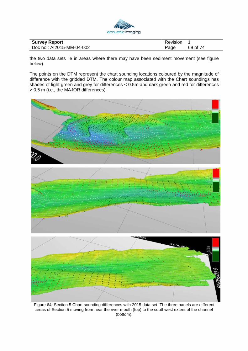
the two data sets lie in areas where there may have been sediment movement (see figure below).
The points on the DTM represent the chart sounding locations coloured by the magnitude of difference with the gridded DTM. The colour map associated with the Chart soundings has shades of light green and grey for differences < 0.5m and dark green and red for differences > 0.5 m (i.e., the MAJOR differences).
Figure 64: Section 5 Chart sounding differences with 2015 data set. The three panels are different areas of Section 5 moving from near the river mouth (top) to the southwest extent of the channel
(bottom).
Survey Report Revision 1 Doc no.: AI2015-MM-04-002 Page 70 of 74
A cluster of “major” differences lies near the mouth of the Skardon River. This is an area with obvious sand waves that could migrate significantly through time.
Other “major” differences lie along the banks of the channel. A sinuous pattern of “major” difference points along the centre of Section 5 suggests the channel thalweg has migrated from 2009 to 2015.
This pattern of major differences in depth between the 2009 and 2015 surveys holds true for the other sections of the river.
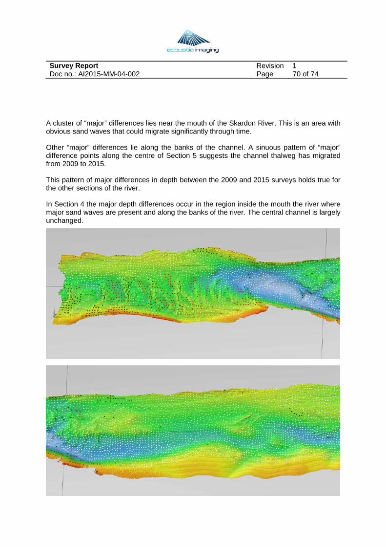
In Section 4 the major depth differences occur in the region inside the mouth the river where major sand waves are present and along the banks of the river. The central channel is largely unchanged.
Survey Report Revision 1 Doc no.: AI2015-MM-04-002 Page 71 of 74
Figure 65: Section 4 Chart sounding differences with 2015 data set.
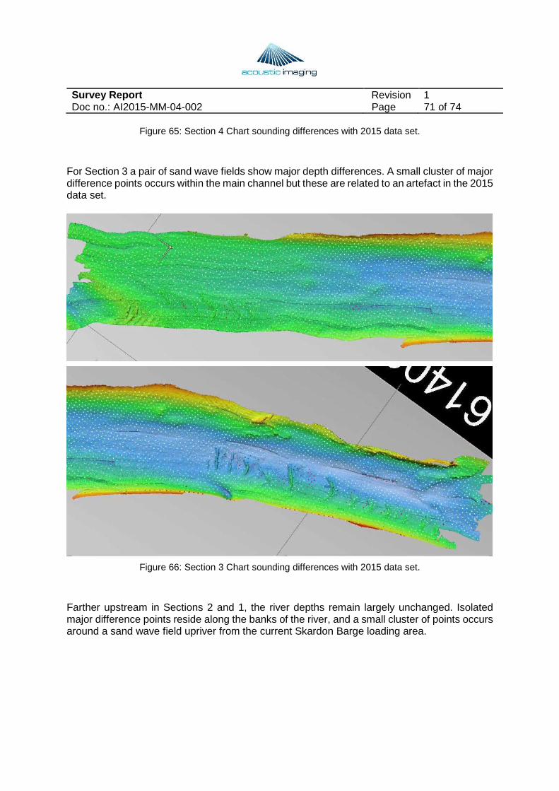
For Section 3 a pair of sand wave fields show major depth differences. A small cluster of major difference points occurs within the main channel but these are related to an artefact in the 2015 data set.
Figure 66: Section 3 Chart sounding differences with 2015 data set.
Farther upstream in Sections 2 and 1, the river depths remain largely unchanged. Isolated major difference points reside along the banks of the river, and a small cluster of points occurs around a sand wave field upriver from the current Skardon Barge loading area.
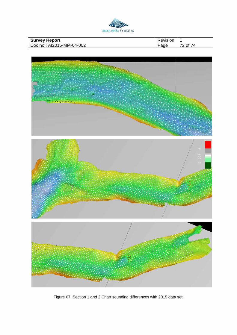
Survey Report Revision 1 Doc no.: AI2015-MM-04-002 Page 72 of 74
Figure 67: Section 1 and 2 Chart sounding differences with 2015 data set.

Survey Report Revision 1 Doc no.: AI2015-MM-04-002 Page 73 of 74
The conclusion to draw from this analysis is that periodic monitoring of river depths will be required for continued safe navigation of vessels as the river bed is changing through time. We suggest a full river survey should be scheduled at the end of the Wet every year, and partial river surveys (e.g., across the channel leading into the river mouth and probably along the length of Section 4) after major storm / flood / tropical cyclone events.
Survey Report Revision 1 Doc no.: AI2015-MM-04-002 Page 74 of 74
8 Summary The April 2015 Skardon River survey as a whole was a great success. A comprehensive data set consisting of MBES bathymetry, SBP seismic, and CTD profiles was obtained across a large stretch of the Skardon River and along a 6km channel offshore of the river mouth. This data set provides invaluable baseline data to use for future cargo loading and barge navigation planning.
The Skardon River is a complex area to conduct hydrographic and geophysical surveys. The interaction between freshwater and saltwater wedges, the unique and ill-defined tidal regime, extreme temperatures, fluctuating weather, and remote location made survey operations complicated.
The April 2015 data set is not perfect, and we have identified a number of improvements to both survey operations and regional infrastructure. Based on our existing analyses, the positioning and orientation data are of high quality and high accuracy. Based on a survey conducted immediately after the April 2015 Skardon River survey, no fundamental problems exist with the dual head MBES system. So any artefacts in the data relate to either the MBES mount, the vessel (e.g., flex of the hull), or the environmental conditions (e.g., a freshwater lens causing beam refraction issues). Continued analysis of the data will lead to further insights on how best to approach surveys into the future.
Of primary importance to future navigation of the Skardon River by loaded barges is the determination LAT in the most rigorous manner possible. The first step in that process is a full analysis of the tidal regime and the installation of tide gauges (as outlined in Section 6.8 of this document) over a suitable period. Given the apparent near-term development in the area, establishing this core infrastructure is of paramount importance.
We have identified a number of regions from the current data set that either bear monitoring into the future or remediation prior to loaded barge navigation (refer to Section 6 of this document). Other areas simply need to be marked on navigation charts as hazards.
Although a challenging area to work, the suite of equipment and software used for the April 2015 survey was entirely appropriate. Improvements in data quality will stem from more informed operational procedures and perhaps a slightly modified processing workflow (that will incorporate the changes to the operational procedures).

Survey Report Revision 1 Doc no.: AI2015-MM-04-002 Page 75 of 74
Appendices
Appendix 1 Example of Daily Report
Appendix 2 Example of Job Safety Analysis
Appendix 3 Example of POSPac Processing Log
Appendix 4 Example of MBES Processing Log
Appendix 5 Statistics comparing 2009 Chart Soundings to April 2015 data
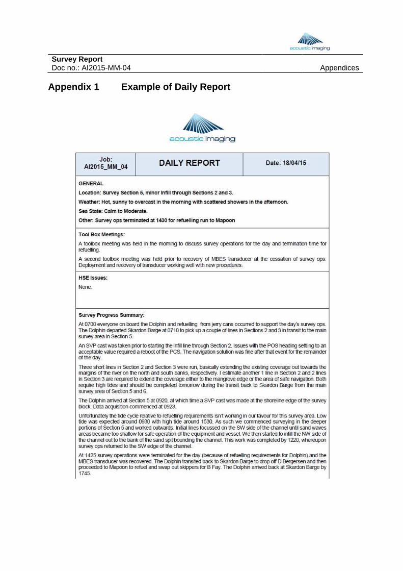
Survey Report Doc no.: AI2015-MM-04 Appendices
Appendix 1 Example of Daily Report
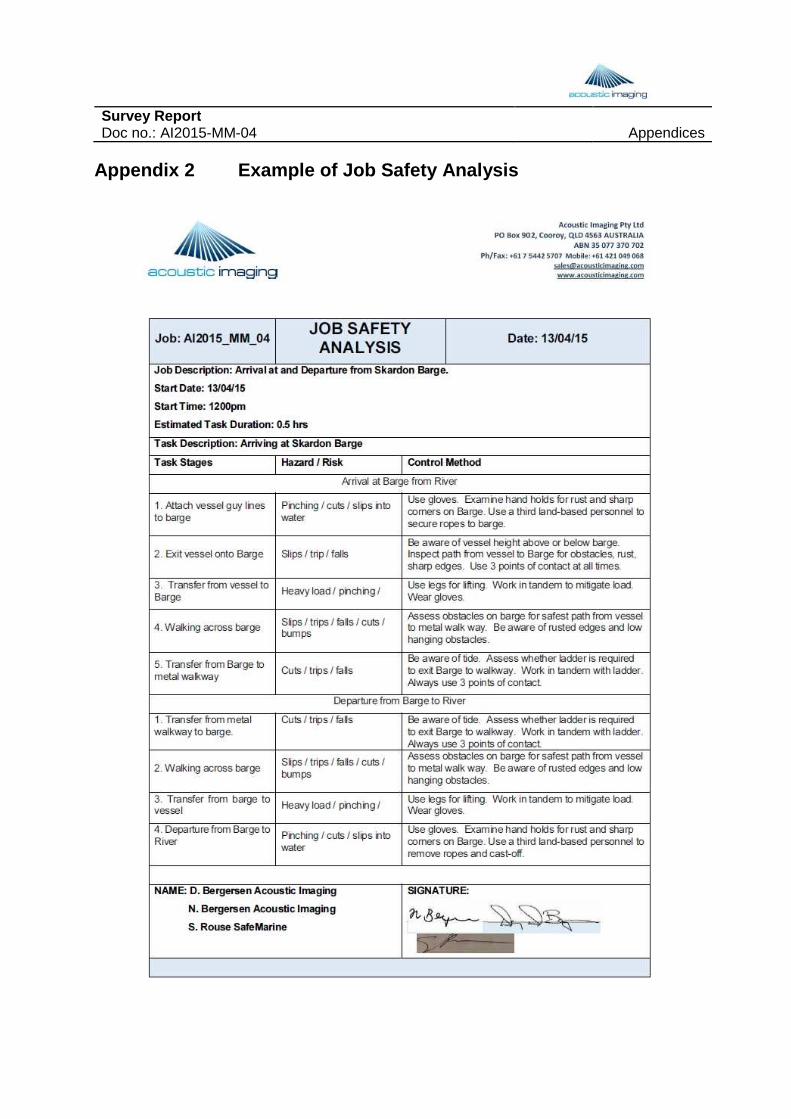
Survey Report Doc no.: AI2015-MM-04 Appendices
Appendix 2 Example of Job Safety Analysis

Survey Report Doc no.: AI2015-MM-04 Appendices
Appendix 3 Example of POSPac Processing Log
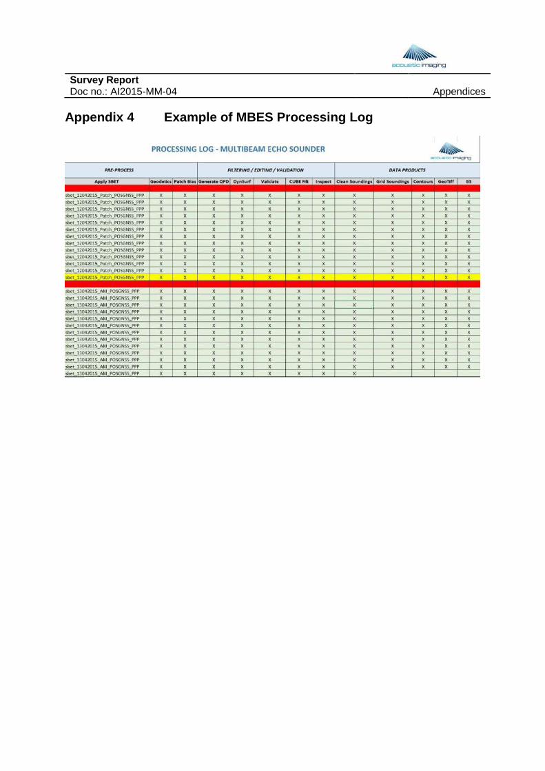
Survey Report Doc no.: AI2015-MM-04 Appendices
Appendix 4 Example of MBES Processing Log
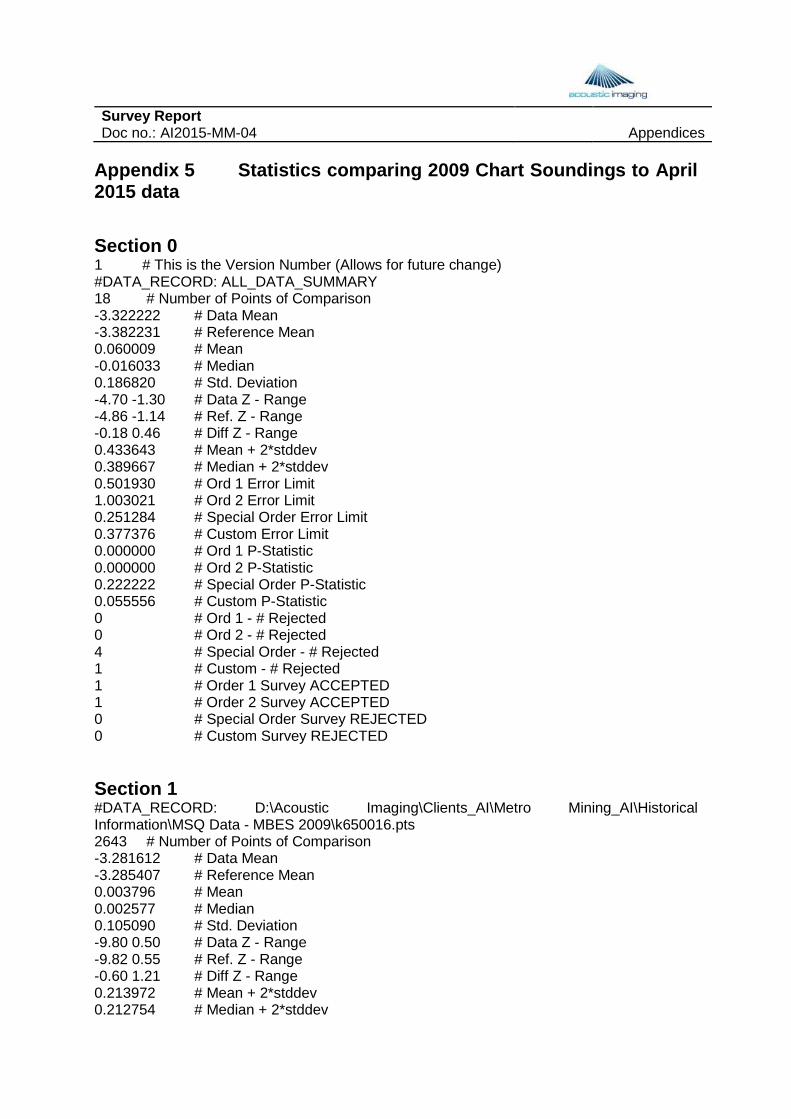
Survey Report Doc no.: AI2015-MM-04 Appendices
Appendix 5 Statistics comparing 2009 Chart Sounding s to April 2015 data
Section 0 1 # This is the Version Number (Allows for future change) #DATA_RECORD: ALL_DATA_SUMMARY 18 # Number of Points of Comparison -3.322222 # Data Mean -3.382231 # Reference Mean 0.060009 # Mean -0.016033 # Median 0.186820 # Std. Deviation -4.70 -1.30 # Data Z - Range -4.86 -1.14 # Ref. Z - Range -0.18 0.46 # Diff Z - Range 0.433643 # Mean + 2*stddev 0.389667 # Median + 2*stddev 0.501930 # Ord 1 Error Limit 1.003021 # Ord 2 Error Limit 0.251284 # Special Order Error Limit 0.377376 # Custom Error Limit 0.000000 # Ord 1 P-Statistic 0.000000 # Ord 2 P-Statistic 0.222222 # Special Order P-Statistic 0.055556 # Custom P-Statistic 0 # Ord 1 - # Rejected 0 # Ord 2 - # Rejected 4 # Special Order - # Rejected 1 # Custom - # Rejected 1 # Order 1 Survey ACCEPTED 1 # Order 2 Survey ACCEPTED 0 # Special Order Survey REJECTED 0 # Custom Survey REJECTED Section 1 #DATA_RECORD: D:\Acoustic Imaging\Clients_AI\Metro Mining_AI\Historical Information\MSQ Data - MBES 2009\k650016.pts 2643 # Number of Points of Comparison -3.281612 # Data Mean -3.285407 # Reference Mean 0.003796 # Mean 0.002577 # Median 0.105090 # Std. Deviation -9.80 0.50 # Data Z - Range -9.82 0.55 # Ref. Z - Range -0.60 1.21 # Diff Z - Range 0.213972 # Mean + 2*stddev 0.212754 # Median + 2*stddev
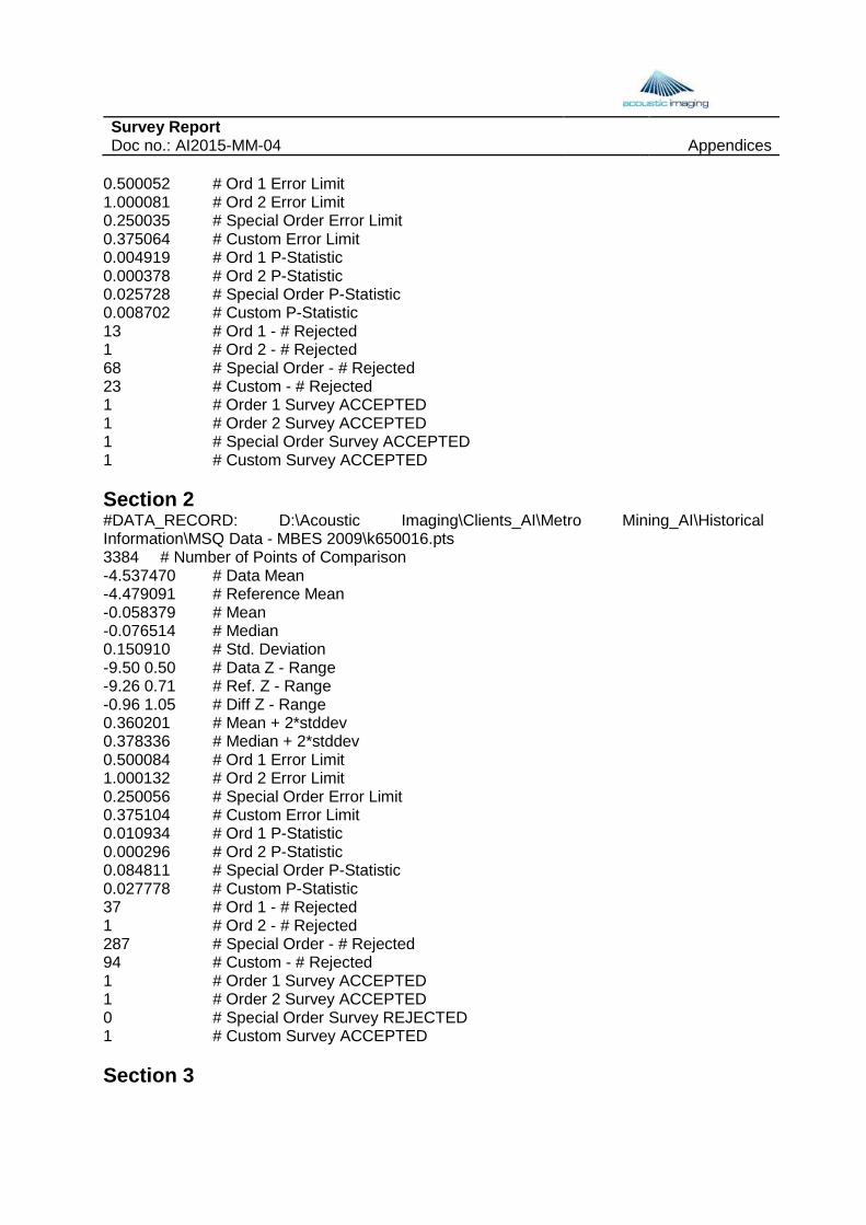
Survey Report Doc no.: AI2015-MM-04 Appendices
0.500052 # Ord 1 Error Limit 1.000081 # Ord 2 Error Limit 0.250035 # Special Order Error Limit 0.375064 # Custom Error Limit 0.004919 # Ord 1 P-Statistic 0.000378 # Ord 2 P-Statistic 0.025728 # Special Order P-Statistic 0.008702 # Custom P-Statistic 13 # Ord 1 - # Rejected 1 # Ord 2 - # Rejected 68 # Special Order - # Rejected 23 # Custom - # Rejected 1 # Order 1 Survey ACCEPTED 1 # Order 2 Survey ACCEPTED 1 # Special Order Survey ACCEPTED 1 # Custom Survey ACCEPTED Section 2 #DATA_RECORD: D:\Acoustic Imaging\Clients_AI\Metro Mining_AI\Historical Information\MSQ Data - MBES 2009\k650016.pts 3384 # Number of Points of Comparison -4.537470 # Data Mean -4.479091 # Reference Mean -0.058379 # Mean -0.076514 # Median 0.150910 # Std. Deviation -9.50 0.50 # Data Z - Range -9.26 0.71 # Ref. Z - Range -0.96 1.05 # Diff Z - Range 0.360201 # Mean + 2*stddev 0.378336 # Median + 2*stddev 0.500084 # Ord 1 Error Limit 1.000132 # Ord 2 Error Limit 0.250056 # Special Order Error Limit 0.375104 # Custom Error Limit 0.010934 # Ord 1 P-Statistic 0.000296 # Ord 2 P-Statistic 0.084811 # Special Order P-Statistic 0.027778 # Custom P-Statistic 37 # Ord 1 - # Rejected 1 # Ord 2 - # Rejected 287 # Special Order - # Rejected 94 # Custom - # Rejected 1 # Order 1 Survey ACCEPTED 1 # Order 2 Survey ACCEPTED 0 # Special Order Survey REJECTED 1 # Custom Survey ACCEPTED Section 3
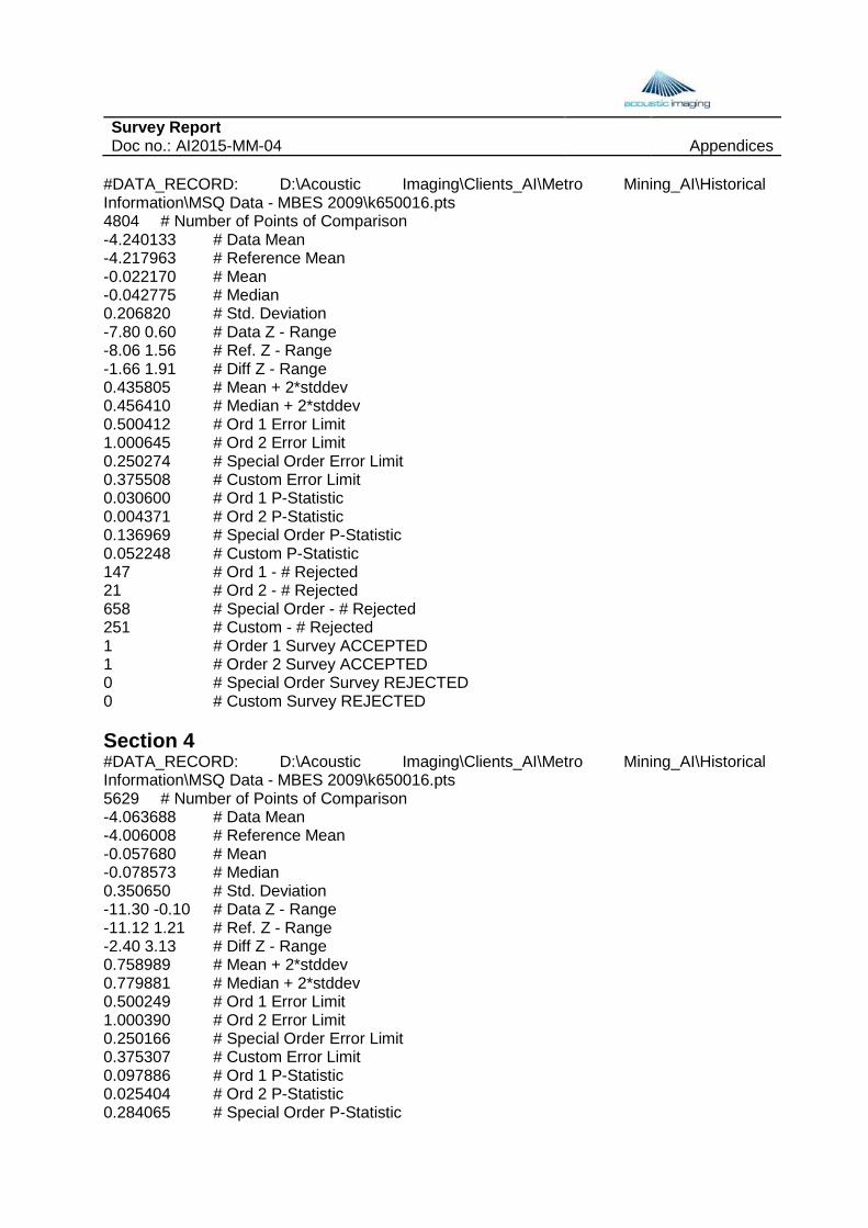
Survey Report Doc no.: AI2015-MM-04 Appendices
#DATA_RECORD: D:\Acoustic Imaging\Clients_AI\Metro Mining_AI\Historical Information\MSQ Data - MBES 2009\k650016.pts 4804 # Number of Points of Comparison -4.240133 # Data Mean -4.217963 # Reference Mean -0.022170 # Mean -0.042775 # Median 0.206820 # Std. Deviation -7.80 0.60 # Data Z - Range -8.06 1.56 # Ref. Z - Range -1.66 1.91 # Diff Z - Range 0.435805 # Mean + 2*stddev 0.456410 # Median + 2*stddev 0.500412 # Ord 1 Error Limit 1.000645 # Ord 2 Error Limit 0.250274 # Special Order Error Limit 0.375508 # Custom Error Limit 0.030600 # Ord 1 P-Statistic 0.004371 # Ord 2 P-Statistic 0.136969 # Special Order P-Statistic 0.052248 # Custom P-Statistic 147 # Ord 1 - # Rejected 21 # Ord 2 - # Rejected 658 # Special Order - # Rejected 251 # Custom - # Rejected 1 # Order 1 Survey ACCEPTED 1 # Order 2 Survey ACCEPTED 0 # Special Order Survey REJECTED 0 # Custom Survey REJECTED Section 4 #DATA_RECORD: D:\Acoustic Imaging\Clients_AI\Metro Mining_AI\Historical Information\MSQ Data - MBES 2009\k650016.pts 5629 # Number of Points of Comparison -4.063688 # Data Mean -4.006008 # Reference Mean -0.057680 # Mean -0.078573 # Median 0.350650 # Std. Deviation -11.30 -0.10 # Data Z - Range -11.12 1.21 # Ref. Z - Range -2.40 3.13 # Diff Z - Range 0.758989 # Mean + 2*stddev 0.779881 # Median + 2*stddev 0.500249 # Ord 1 Error Limit 1.000390 # Ord 2 Error Limit 0.250166 # Special Order Error Limit 0.375307 # Custom Error Limit 0.097886 # Ord 1 P-Statistic 0.025404 # Ord 2 P-Statistic 0.284065 # Special Order P-Statistic
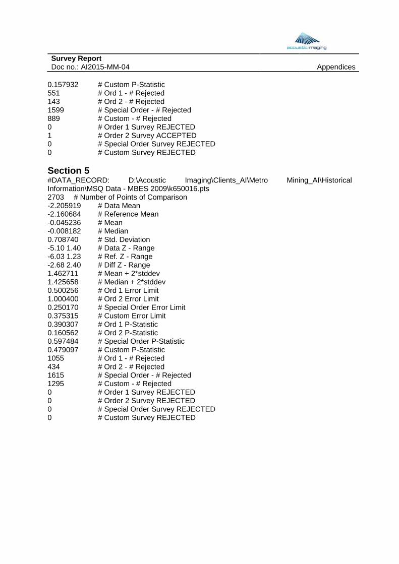
Survey Report Doc no.: AI2015-MM-04 Appendices
0.157932 # Custom P-Statistic 551 # Ord 1 - # Rejected 143 # Ord 2 - # Rejected 1599 # Special Order - # Rejected 889 # Custom - # Rejected 0 # Order 1 Survey REJECTED 1 # Order 2 Survey ACCEPTED 0 # Special Order Survey REJECTED 0 # Custom Survey REJECTED Section 5 #DATA_RECORD: D:\Acoustic Imaging\Clients_AI\Metro Mining_AI\Historical Information\MSQ Data - MBES 2009\k650016.pts 2703 # Number of Points of Comparison -2.205919 # Data Mean -2.160684 # Reference Mean -0.045236 # Mean -0.008182 # Median 0.708740 # Std. Deviation -5.10 1.40 # Data Z - Range -6.03 1.23 # Ref. Z - Range -2.68 2.40 # Diff Z - Range 1.462711 # Mean + 2*stddev 1.425658 # Median + 2*stddev 0.500256 # Ord 1 Error Limit 1.000400 # Ord 2 Error Limit 0.250170 # Special Order Error Limit 0.375315 # Custom Error Limit 0.390307 # Ord 1 P-Statistic 0.160562 # Ord 2 P-Statistic 0.597484 # Special Order P-Statistic 0.479097 # Custom P-Statistic 1055 # Ord 1 - # Rejected 434 # Ord 2 - # Rejected 1615 # Special Order - # Rejected 1295 # Custom - # Rejected 0 # Order 1 Survey REJECTED 0 # Order 2 Survey REJECTED 0 # Special Order Survey REJECTED 0 # Custom Survey REJECTED