Correction of Bathymetric Survey Artifacts Resulting Apparent Wave-Induced Vertical Position of an AUV Val Schmidt, Nicole Raineault, Adam Skarke, Art Trembanis, Larry Mayer 1 October, 2010 Version 2

Introduction Recent increases in the capability and reliability of autonomous underwater vehicles (AUVs) have provided the opportunity to conduct bathymetric seafloor surveys in shallow water (< 50 m). Unfortunately, surveys of this water depth may contain artifacts induced by large amplitude wave motion at the surface. The artifacts occur when an on-board pressure sensor determines the depth of the AUV. Waves overhead induce small pressure fluctuations at depth, which modulate the AUV’s pressure sensor output without causing actual vertical movement of the AUV. Since bathymetric measurements are made with respect to the AUV’s depth, these pressure fluctuations, in turn, modulate the measurement of the seafloor. The result is a periodic across-track, vertical offset of the seafloor profile (similar to a heave artifact sometimes common in surface vessel surveys). In this paper we describe our experience with the “Gavia” model AUV (Hafmynd EHF, Iceland) in a recent bathymetric survey during which wave action overhead induced such an artifact with a peak-to-peak amplitude as large as 1 meter. A method for removing the artifact as well as recommendations for modifications to the sonar, INS and AUV to mitigate the effect in the future are provided. A brief note on terminology: The term “heave” as used in this paper is defined as the vertical displacement of the AUV with respect to the surface (the AUV’s depth). This convention is used in surface ship surveying and in the AUV’s Geoacoustics bathymetric sonar. Unfortunately, the term “heave” is defined by the AUV’s inertial navigation system and internal logs as vertical velocity of the AUV. Every effort will be made to reduce confusion between these definitions.

The Gavia The Gavia is a modular AUV having the ability to tailor the module make-up for a given mission (Figure 1.). The system used in this study included a “Geoswath” 500kHz, phase-measuring bathymetric sonar (PMBS) module from Geoacoustics (Kongsberg), a navigation module combining a 1200 kHz doppler-velocity log (DVL) from RD Instruments and a SEANAV T-24 inertial navigation system (INS) from Kearfott. While submerged, the AUV operates independently of any external navigation system, relying on DVL and INS operation completely.

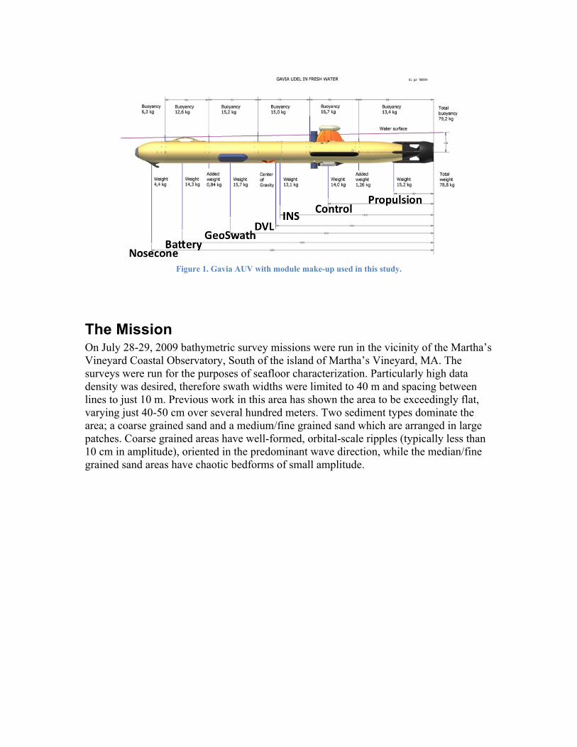
Figure 1. Gavia AUV with module make-up used in this study.

The Mission On July 28-29, 2009 bathymetric survey missions were run in the vicinity of the Martha’s Vineyard Coastal Observatory, South of the island of Martha’s Vineyard, MA. The surveys were run for the purposes of seafloor characterization. Particularly high data density was desired, therefore swath widths were limited to 40 m and spacing between lines to just 10 m. Previous work in this area has shown the area to be exceedingly flat, varying just 40-50 cm over several hundred meters. Two sediment types dominate the area; a coarse grained sand and a medium/fine grained sand which are arranged in large patches. Coarse grained areas have well-formed, orbital-scale ripples (typically less than 10 cm in amplitude), oriented in the predominant wave direction, while the median/fine grained sand areas have chaotic bedforms of small amplitude.

Figure 2 Survey track of the Gavia AUV.

When operating the AUV for seafloor surveys the Gavia is placed in bottom-tracking mode to maximize the quality of the resulting bathymetry. In this mode, the AUV maintains a constant depth above the bottom, as measured by the INS (with DVL input). An altitude of 6 meters was maintained for this survey. Total water depth in the survey area is 11 to 13 meters. Nominal survey speed for the AUV was 1.7 m/s through water. A west-to-east current of ~0.5 m/s resulted in speeds over ground generally between 1.2 and 2.3 m/s.

Results Initial processing of the swath bathymetry data was conducted using both the Geoacoustics GS+ processing suite and separately by an internally developed set of MATLAB tools. Both processing options filter the data for outliers, georeference each sounding and finally grid (and perhaps smooth) these into a final surface. The MATLAB software does not currently correct for refraction of the acoustic signals in the water column, however errors due to that omission are separate and distinct from the artifacts discussed here. Results on one swath of sonar data processing with MATLAB are shown in Figure 3.

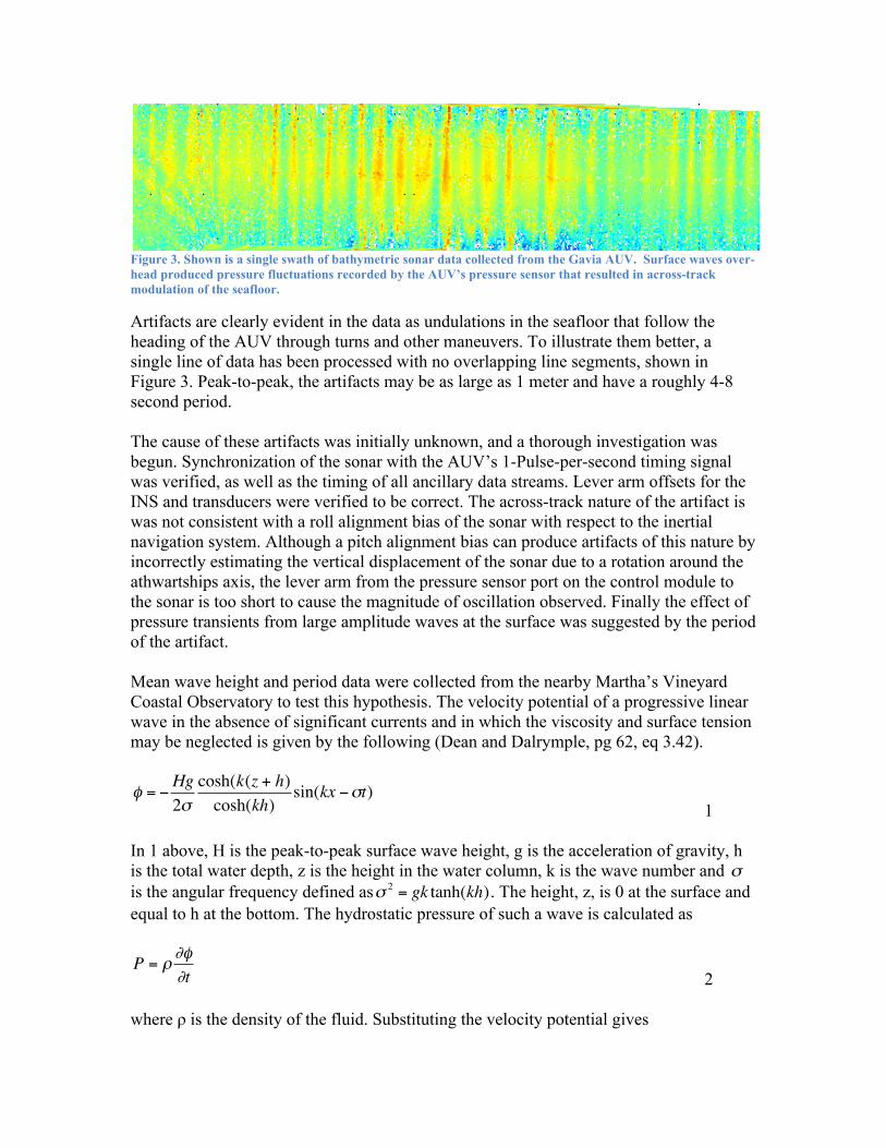
Figure 3. Shown is a single swath of bathymetric sonar data collected from the Gavia AUV. Surface waves over-head produced pressure fluctuations recorded by the AUV’s pressure sensor that resulted in across-track modulation of the seafloor.

Artifacts are clearly evident in the data as undulations in the seafloor that follow the heading of the AUV through turns and other maneuvers. To illustrate them better, a single line of data has been processed with no overlapping line segments, shown in Figure 3. Peak-to-peak, the artifacts may be as large as 1 meter and have a roughly 4-8 second period. The cause of these artifacts was initially unknown, and a thorough investigation was begun. Synchronization of the sonar with the AUV’s 1-Pulse-per-second timing signal was verified, as well as the timing of all ancillary data streams. Lever arm offsets for the INS and transducers were verified to be correct. The across-track nature of the artifact is was not consistent with a roll alignment bias of the sonar with respect to the inertial navigation system. Although a pitch alignment bias can produce artifacts of this nature by incorrectly estimating the vertical displacement of the sonar due to a rotation around the athwartships axis, the lever arm from the pressure sensor port on the control module to the sonar is too short to cause the magnitude of oscillation observed. Finally the effect of pressure transients from large amplitude waves at the surface was suggested by the period of the artifact. Mean wave height and period data were collected from the nearby Martha’s Vineyard Coastal Observatory to test this hypothesis. The velocity potential of a progressive linear wave in the absence of significant currents and in which the viscosity and surface tension may be neglected is given by the following (Dean and Dalrymple, pg 62, eq 3.42).

€

φ = −Hg2σ

cosh(k(z + h)cosh(kh)

sin(kx −σt) 1

In 1 above, H is the peak-to-peak surface wave height, g is the acceleration of gravity, h is the total water depth, z is the height in the water column, k is the wave number and

€

σ is the angular frequency defined as

€

σ 2 = gk tanh(kh). The height, z, is 0 at the surface and equal to h at the bottom. The hydrostatic pressure of such a wave is calculated as

€

P = ρ∂φ∂t 2

where ρ is the density of the fluid. Substituting the velocity potential gives

€

P =H2gρ cosh(k(h + z))

cosh(kh)cos(kx −σt)

3

The amplitude of the pressure oscillation felt by the AUV at a depth, z, due to surface swell of peak-to-peak amplitude H is then given by

€

P =H2gρ cosh(k(h + z))

cosh(kh) 4

The hydrostatic pressure due to a column of water of depth z’ above the AUV is given by

€

P = ρgz' 5 Therefore we may equate Equations 4 and 5 and calculate the error in AUV’s depth estimate introduced by surface swell as a function of the AUV’s depth, z, and the swell height, H. The depth error, z’ is then

€

z'= H2cosh(k(h + z))cosh(kh) 6

Wave data from the Martha’s Vineyard Coastal Observatory were obtained from the period the survey was conducted. Wave height (average crest to trough height of the one-third highest waves) is plotted in Figure 3 showing values from 3-6 feet. Wave period is plotted in Figure 4, showing values of 4-6 seconds.

Figure 3. Wave height for the week of July 26-Aug 1, 2009

Figure 4. Wave period for the week of July 26-Aug 1 2009 as observed by the MVCO.

The wavelength can be calculated from the following relations for wave speed, c wave number, k and wave period, T,

€

c 2 =σ 2

k 2,

€

k =2πλ

,

€

λ =cT 7

Substituting the expression for the angular velocity,

€

σ , from above into the first equation gives

€

c 2 =gtanh(kh)

k 8

We consider the case in which the wavelength,

€

λ , is much greater then the water depth, h. Under these circumstances

€

tan(kh) ≈1, and the expression becomes

€

c 2 =gk 9

Combining the remaining equations and solving for wavelength gives

€

λ =gT 2

2π 10

Substituting values from the Martha’s Vineyard Coastal Observatory data for wave period (5 s) and wave height (4ft, 1.2 m) into the equations for wavelength,

€

λ , and depth error expression,

€

ʹ′ z , gives the depth error profile plotted in Figure 5.

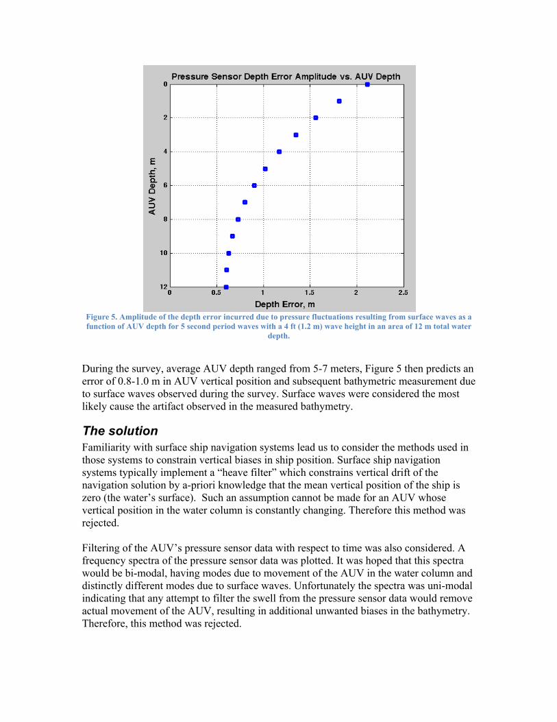
Figure 5. Amplitude of the depth error incurred due to pressure fluctuations resulting from surface waves as a function of AUV depth for 5 second period waves with a 4 ft (1.2 m) wave height in an area of 12 m total water

depth.

During the survey, average AUV depth ranged from 5-7 meters, Figure 5 then predicts an error of 0.8-1.0 m in AUV vertical position and subsequent bathymetric measurement due to surface waves observed during the survey. Surface waves were considered the most likely cause the artifact observed in the measured bathymetry.

The solution Familiarity with surface ship navigation systems lead us to consider the methods used in those systems to constrain vertical biases in ship position. Surface ship navigation systems typically implement a “heave filter” which constrains vertical drift of the navigation solution by a-priori knowledge that the mean vertical position of the ship is zero (the water’s surface). Such an assumption cannot be made for an AUV whose vertical position in the water column is constantly changing. Therefore this method was rejected. Filtering of the AUV’s pressure sensor data with respect to time was also considered. A frequency spectra of the pressure sensor data was plotted. It was hoped that this spectra would be bi-modal, having modes due to movement of the AUV in the water column and distinctly different modes due to surface waves. Unfortunately the spectra was uni-modal indicating that any attempt to filter the swell from the pressure sensor data would remove actual movement of the AUV, resulting in additional unwanted biases in the bathymetry. Therefore, this method was rejected.

Altitude above the sea floor as measured from the AUV’s DVL was considered as a method to constrain the movement of the AUV in the water column such that oscillations in the pressure signal due to swell could be isolated from those due to the AUV’s movement. This method was also rejected, as it requires a-priori knowledge of the bathymetry. As the investigation ensured, the following details about the AUV’s operation and subsystems were learned:

• The control module’s pressure sensor serial output is captured by a “Rabbit” electronics board, which reformats the data, converts it to depth and subsequently broadcasts it on the AUV’s internal Ethernet network. Density of the seawater is not considered in this calculation.

• The Geoswath sonar passively monitors the AUV’s internal network, capturing pressure data packets, time stamping them and recording them in the “AUX1” data channel within the sonar’s RDF data file.

• In post-processing, the GS+ software utilizes the depth recorded in the AUX1 channel as the depth from which all subsequent sonar measurements are reported by default.

• The Geoswath maintains a sense of time by time-stamping the receipt of a 1-PPS signal provided by the AUV’s GPS unit. (This signal is generated even after the AUV submerges and no further GPS fixes are obtained.) The timestamp is compared to that received by a subsequent ASCII timing message from the INS. The Geoswath then step-corrects its clock to the 1-PPS signal.

• The SEANAV INS serial output is received by its own Rabbit electronics board. This Rabbit board reformats the SEANAV data for (at least) two purposes. One message is broadcast to the Geoswath. A second message is sent to the control module for navigation. (Both via Ethernet.)

• The term “heave,” as defined by the Seanav output message, is the vertical velocity of the AUV. The “heave” field, as defined in the MRU message sent from the rabbit board in the Seanav is vertical position, however this field is set to zero.

• The SEANAV’s estimate of the depth of the AUV is derived from its own internal sensors and the control module’s pressure measurement. Double integration of the INS accelerometers, combined with single integration of the vertical component of the DVL produce a real-time depth estimate. This depth estimate is then constrained by depth input from the pressure sensor through a “second-order, critically damped, feedback loop having a 100 second time constant” (Don Weber, Kearfott).

From this information, it was seen that the SEANAV inertial navigation system should capture real vertical movements of the AUV in the water column. Because the pressure-depth feedback loop had been implemented with a 100-second time constant, variations in the pressure sensor occurring over periods less than 100 seconds should be removed. Therefore surface wave action having a period of 4-6 seconds would be completely removed from the SEANAV’s depth estimate.

To test the hypothesis, the SEANAV depth estimate was substituted for the pressure sensor depth in the post-processing of Geoswath data files. To accomplish this substitution, new ASCII text attitude files containing a time stamp, pitch, roll and heave were imported and applied to the Geoswath data using the GS+ software suite. These files were generated by first extracting the pitch and roll measurements with their associated time stamps from the original RDF data files. SEANAV depth records recorded by the Gavia’s internal logging system were then corrected for a time stamp offset and then interpolated to the RDF attitude time stamps. Finally the original time stamps, pitch, roll and the new heave values derived from the SEANAV depth estimate were used for subsequent manual processing in MATLAB or written to new attitude files and imported into GS+.

Figure 6. Seafloor bathymetry with surface wave artifact (top) and after use of Seanav provided depth (bottom). Both plots have identical color scales – red-to-blue approximately 1 m.

The result of substituting the SEANAV depth estimate for the pressure sensor depth is shown in Figure 6 along with the original plot. Artifacts attributed to surface wave motion are nearly completely removed. Some residual swell artifacts remain and are likely to result from the a failure of the Gavia’s logging system to capture depth data at a rate meeting the Nyquist sample criteria for the artifact-causing pressure fluctuations. Although Gavia’s standard logging system provides depth values at 0.5 Hz intervals, recent (2010) upgrades to the unit allow for raw recording of the binary SEANAV data stream providing depth estimates at 20 Hz. This rate is expected to provide sufficient bandwidth for most situations.

Figure 7 Grid of bathymetric data when the SEANAV depth estimate has been used in lieu of the pressure sensor measurement. The profile below along the line drawn on the grid shows relief spanning only 10 cm, consistent with previous surveys in the area.

A grid created from the full bathymetric data set is shown in Figure 7. Sand wave ripples in areas of fine-grained sand, which were previously occluded by the swell artifact, are now clearly evident.

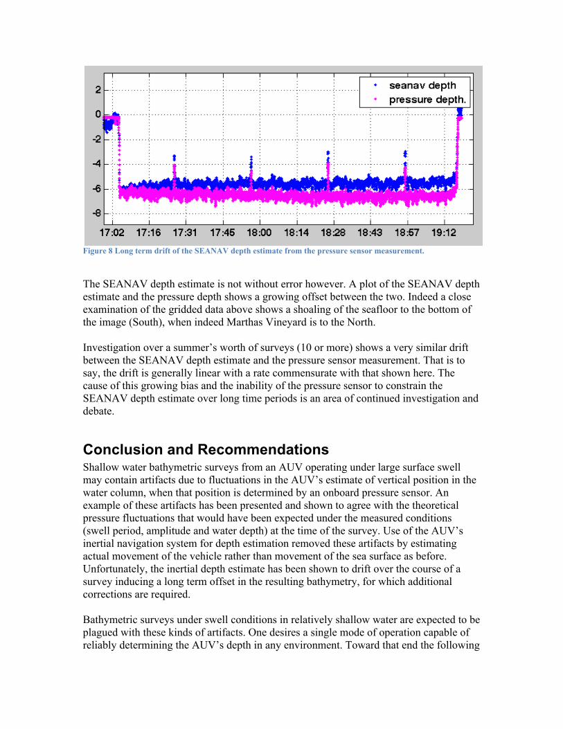
Figure 8 Long term drift of the SEANAV depth estimate from the pressure sensor measurement.

The SEANAV depth estimate is not without error however. A plot of the SEANAV depth estimate and the pressure depth shows a growing offset between the two. Indeed a close examination of the gridded data above shows a shoaling of the seafloor to the bottom of the image (South), when indeed Marthas Vineyard is to the North. Investigation over a summer’s worth of surveys (10 or more) shows a very similar drift between the SEANAV depth estimate and the pressure sensor measurement. That is to say, the drift is generally linear with a rate commensurate with that shown here. The cause of this growing bias and the inability of the pressure sensor to constrain the SEANAV depth estimate over long time periods is an area of continued investigation and debate.

Conclusion and Recommendations Shallow water bathymetric surveys from an AUV operating under large surface swell may contain artifacts due to fluctuations in the AUV’s estimate of vertical position in the water column, when that position is determined by an onboard pressure sensor. An example of these artifacts has been presented and shown to agree with the theoretical pressure fluctuations that would have been expected under the measured conditions (swell period, amplitude and water depth) at the time of the survey. Use of the AUV’s inertial navigation system for depth estimation removed these artifacts by estimating actual movement of the vehicle rather than movement of the sea surface as before. Unfortunately, the inertial depth estimate has been shown to drift over the course of a survey inducing a long term offset in the resulting bathymetry, for which additional corrections are required. Bathymetric surveys under swell conditions in relatively shallow water are expected to be plagued with these kinds of artifacts. One desires a single mode of operation capable of reliably determining the AUV’s depth in any environment. Toward that end the following

recommendations are suggested for the Gavia AUV outfitted with a Kearfott SEANAV INS as used in this survey.

1. Injection of the SEANAV depth estimate for the “heave” field in data supplied to the Geoswath sonar in real-time (this value is currently zero). In addition, modification of the GS+ processing suite to accept the heave field in lieu of the “AUX1” pressure depth by default. Drift of the SEANAV depth estimate from the mean pressure depth will require an additional correction. The offset of the mean SEANAV depth estimate to the mean pressure measurement at the end of the mission (when the AUV returns to the surface) should provide a reasonable estimate of the linear drift rate. The drift corrector than then be calculated from this drift rate over the duration of the mission and applied to the data, perhaps along with the tidal correction.

2. The SEANAV pressure feedback loop should be further investigated and perhaps modified to further constrain the SEANAV depth estimate to the long-term pressure average. Initial discussions with Kearfott indicate that the current behavior of the feedback loop may be as designed. None-the-less, for hydrographic applications it is inadequate to sufficiently constrain the AUV’s position in the water column alone.

References [1] R.G. Dean and R.A. Dalrymple, Water wave mechanics for engineers and scientists, World Scientific,

1991.