Embed Size (px)
Citation preview
Metrics, Analysis, and Examples
Performance Analysis
Spring 2018 © CS 438 Staff - University of Illinois 1
Spring 2018 © CS 438 Staff - University of Illinois 2
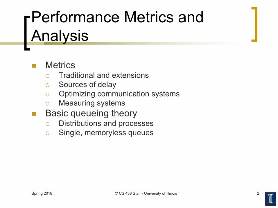
Performance Metrics and Analysis
n Metrics¡ Traditional and extensions¡ Sources of delay¡ Optimizing communication systems¡ Measuring systems
n Basic queueing theory¡ Distributions and processes¡ Single, memoryless queues
Spring 2018 © CS 438 Staff - University of Illinois 3
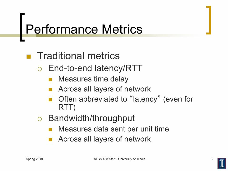
Performance Metrics
n Traditional metrics¡ End-to-end latency/RTT
n Measures time delayn Across all layers of networkn Often abbreviated to �latency� (even for
RTT)¡ Bandwidth/throughput
n Measures data sent per unit timen Across all layers of network
Spring 2018 © CS 438 Staff - University of Illinois 4
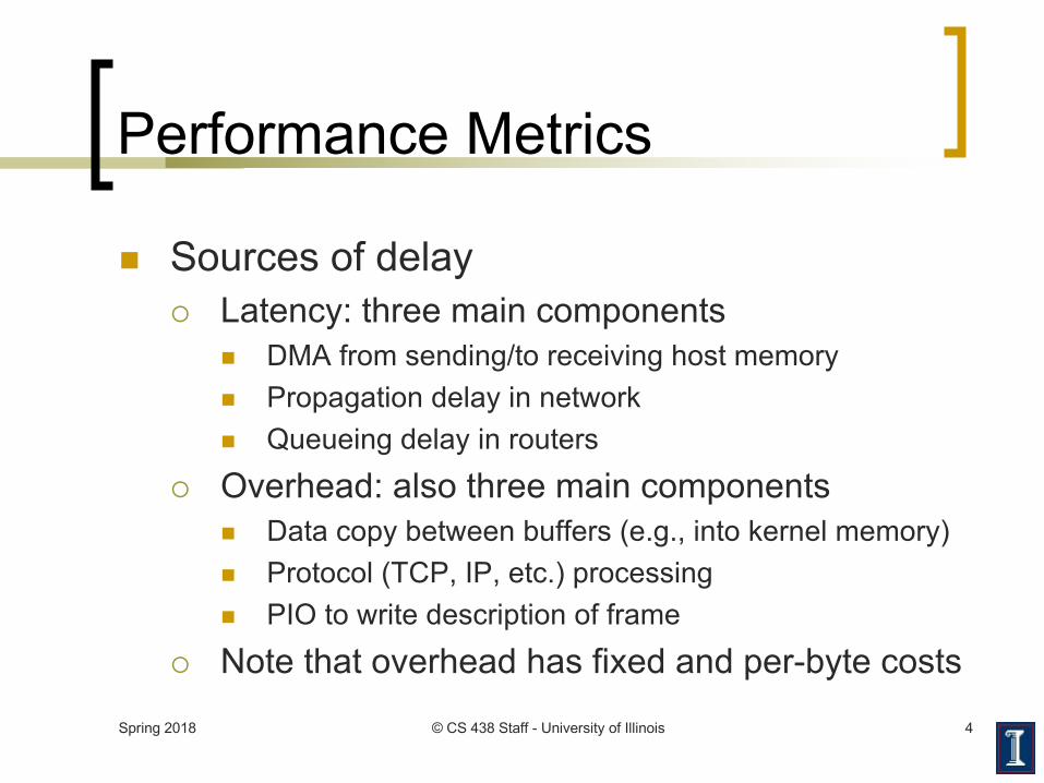
Performance Metrics
n Sources of delay
¡ Latency: three main components
n DMA from sending/to receiving host memory
n Propagation delay in network
n Queueing delay in routers
¡ Overhead: also three main components
n Data copy between buffers (e.g., into kernel memory)
n Protocol (TCP, IP, etc.) processing
n PIO to write description of frame
¡ Note that overhead has fixed and per-byte costs

Spring 2018 © CS 438 Staff - University of Illinois 5
Performance Metrics
n Optimizing communication systems¡ Optimize the common case
n Send/receive usually more important than connection setup/teardown¡ TCP header changes little between segments¡ Often only a few connections at end hosts
n Minimize context switchesn Minimize copying of data
Spring 2018 © CS 438 Staff - University of Illinois 6
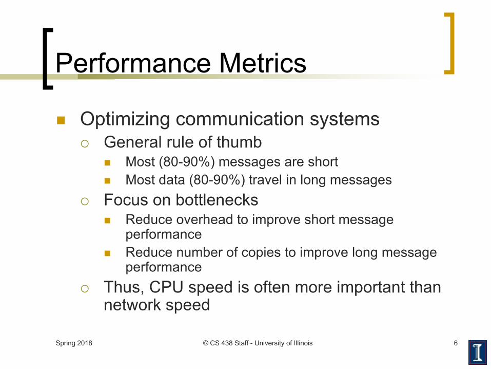
Performance Metrics
n Optimizing communication systems¡ General rule of thumb
n Most (80-90%) messages are shortn Most data (80-90%) travel in long messages
¡ Focus on bottlenecksn Reduce overhead to improve short message
performancen Reduce number of copies to improve long message
performance¡ Thus, CPU speed is often more important than
network speed
Spring 2018 © CS 438 Staff - University of Illinois 7
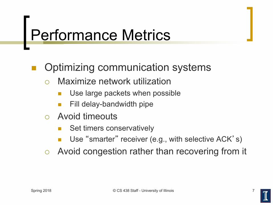
Performance Metrics
n Optimizing communication systems¡ Maximize network utilization
n Use large packets when possiblen Fill delay-bandwidth pipe
¡ Avoid timeoutsn Set timers conservativelyn Use �smarter� receiver (e.g., with selective ACK�s)
¡ Avoid congestion rather than recovering from it
Spring 2018 © CS 438 Staff - University of Illinois 8
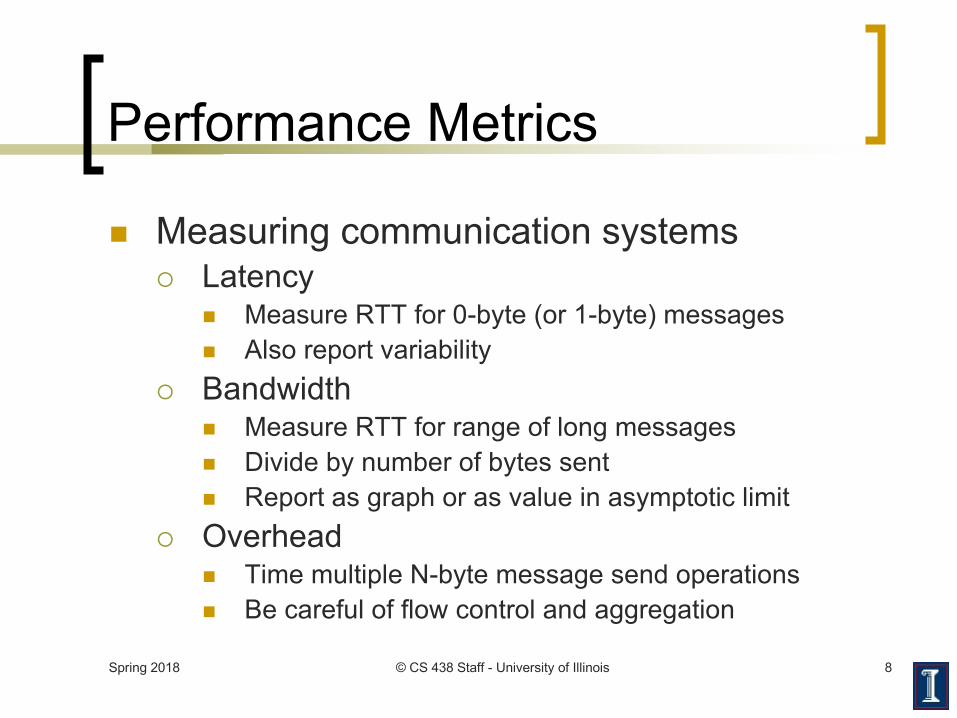
Performance Metrics
n Measuring communication systems¡ Latency
n Measure RTT for 0-byte (or 1-byte) messagesn Also report variability
¡ Bandwidthn Measure RTT for range of long messagesn Divide by number of bytes sentn Report as graph or as value in asymptotic limit
¡ Overheadn Time multiple N-byte message send operationsn Be careful of flow control and aggregation
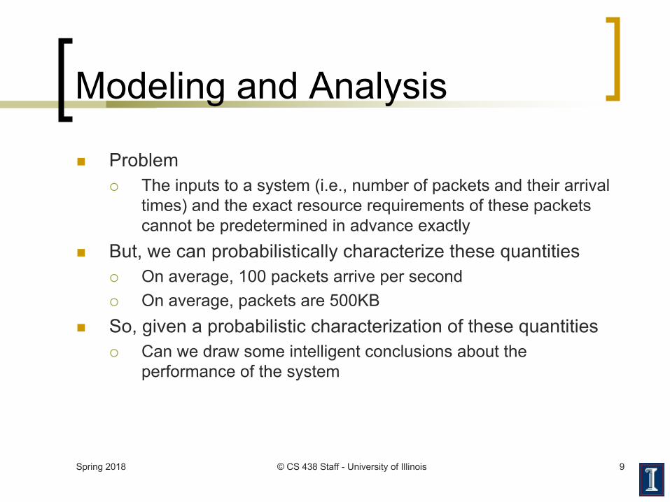
Modeling and Analysis
n Problem¡ The inputs to a system (i.e., number of packets and their arrival
times) and the exact resource requirements of these packets cannot be predetermined in advance exactly
n But, we can probabilistically characterize these quantities¡ On average, 100 packets arrive per second¡ On average, packets are 500KB
n So, given a probabilistic characterization of these quantities¡ Can we draw some intelligent conclusions about the
performance of the system
Spring 2018 © CS 438 Staff - University of Illinois 9
Spring 2018 © CS 438 Staff - University of Illinois 10
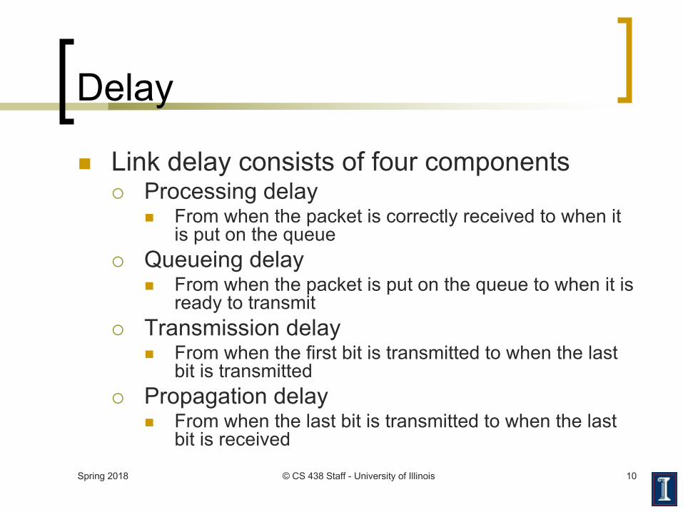
Delay
n Link delay consists of four components¡ Processing delay
n From when the packet is correctly received to when it is put on the queue
¡ Queueing delayn From when the packet is put on the queue to when it is
ready to transmit¡ Transmission delay
n From when the first bit is transmitted to when the last bit is transmitted
¡ Propagation delayn From when the last bit is transmitted to when the last
bit is received
Spring 2018 © CS 438 Staff - University of Illinois 11
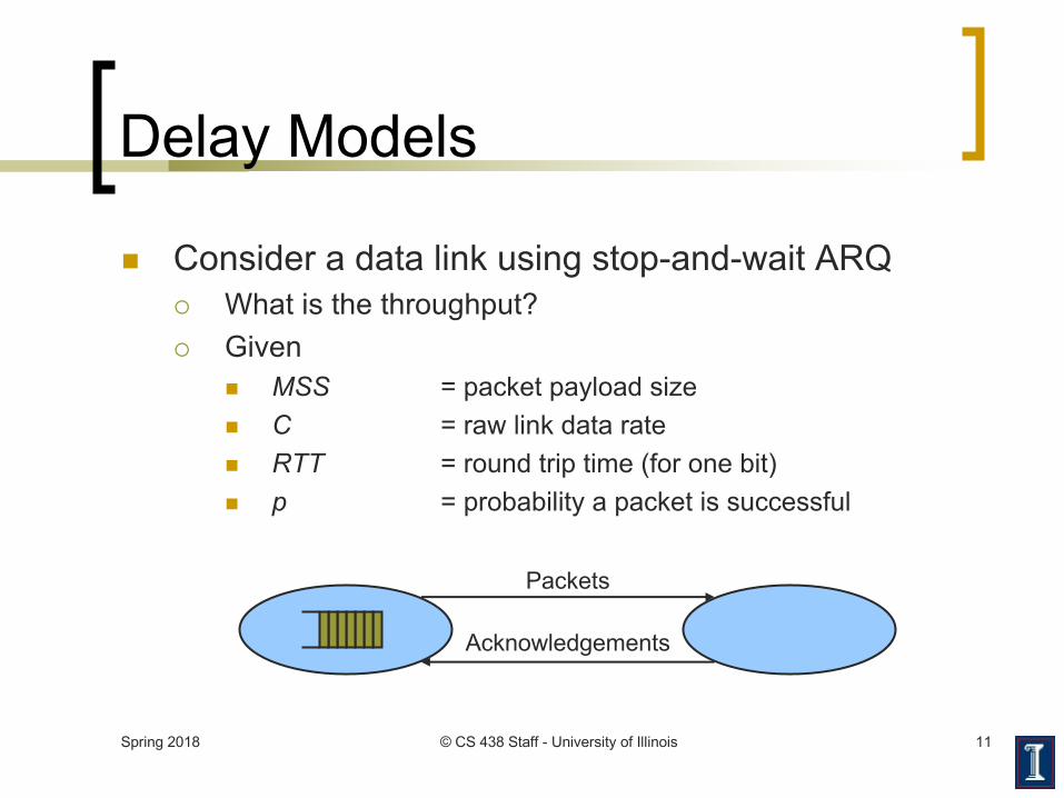
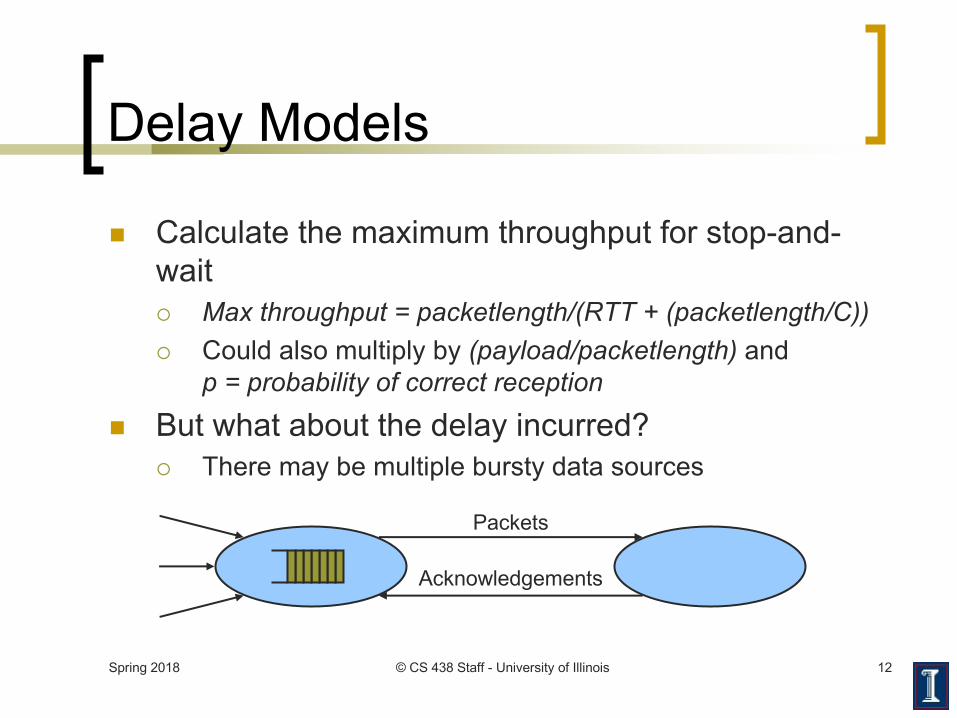
Delay Models
n Consider a data link using stop-and-wait ARQ¡ What is the throughput?¡ Given
n MSS = packet payload sizen C = raw link data raten RTT = round trip time (for one bit)n p = probability a packet is successful
Packets
Acknowledgements
Spring 2018 © CS 438 Staff - University of Illinois 12
Delay Models
n Calculate the maximum throughput for stop-and-wait¡ Max throughput = packetlength/(RTT + (packetlength/C))¡ Could also multiply by (payload/packetlength) and
p = probability of correct reception
n But what about the delay incurred?¡ There may be multiple bursty data sources
Packets
Acknowledgements
Spring 2018 © CS 438 Staff - University of Illinois 13
Basic Queueing Theory
n Elementary notions¡ Things arrive at a queue according to some
probability distribution¡ Things leave a queue according to a second
probability distribution¡ Averaged over time
n Things arriving and things leaving must be equaln Or the queue length will grow without bound
¡ Convenient to express probability distributions as average rates
Spring 2018 © CS 438 Staff - University of Illinois 14
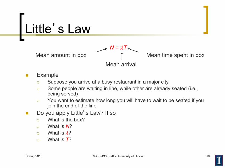
Little�s Law
n Goal¡ Estimate relevant values
n Average number of customers in the system¡ The number of customers either waiting in queue or receiving
servicen Average delay per customer
¡ The time a customer spends waiting plus the service time¡ In terms of known values
n Customer arrival rate¡ The number of customers entering the system per unit time
n Customer service rate¡ The number of customers the system serves per unit time
Spring 2018 © CS 438 Staff - University of Illinois 15
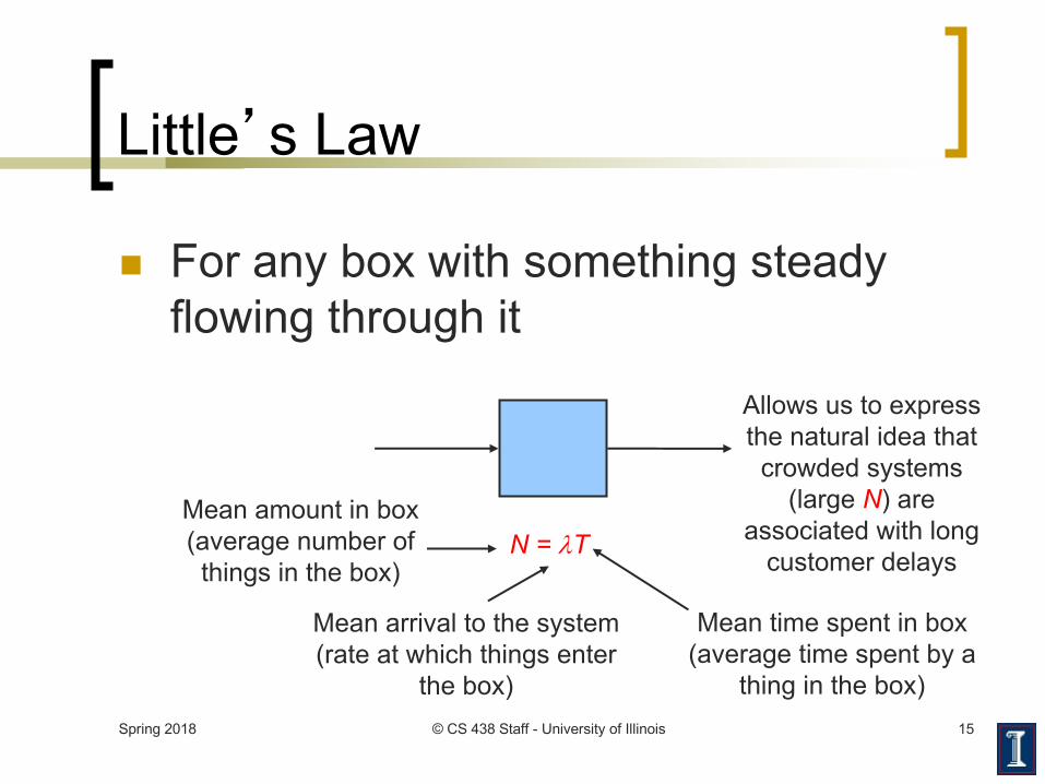
Little�s Law
n For any box with something steady flowing through it
N = lTMean amount in box(average number of things in the box)
Mean time spent in box (average time spent by a
thing in the box)
Mean arrival to the system(rate at which things enter
the box)
Allows us to express the natural idea that crowded systems
(large N) are associated with long
customer delays
Spring 2018 © CS 438 Staff - University of Illinois 16
Little�s Law
n Example¡ Suppose you arrive at a busy restaurant in a major city¡ Some people are waiting in line, while other are already seated (i.e.,
being served)¡ You want to estimate how long you will have to wait to be seated if you
join the end of the linen Do you apply Little�s Law? If so
¡ What is the box?¡ What is N?¡ What is l?¡ What is T?
N = lTMean amount in box Mean time spent in box
Mean arrival
Spring 2018 © CS 438 Staff - University of Illinois 17
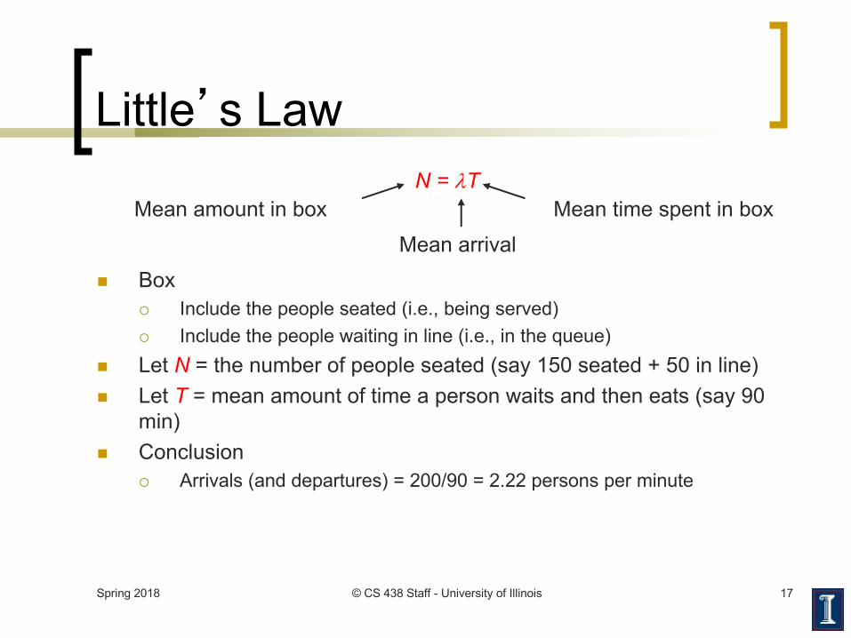
Little�s Law
n Box¡ Include the people seated (i.e., being served)¡ Include the people waiting in line (i.e., in the queue)
n Let N = the number of people seated (say 150 seated + 50 in line)n Let T = mean amount of time a person waits and then eats (say 90
min)n Conclusion
¡ Arrivals (and departures) = 200/90 = 2.22 persons per minute
N = lTMean amount in box Mean time spent in box
Mean arrival
Spring 2018 © CS 438 Staff - University of Illinois 18
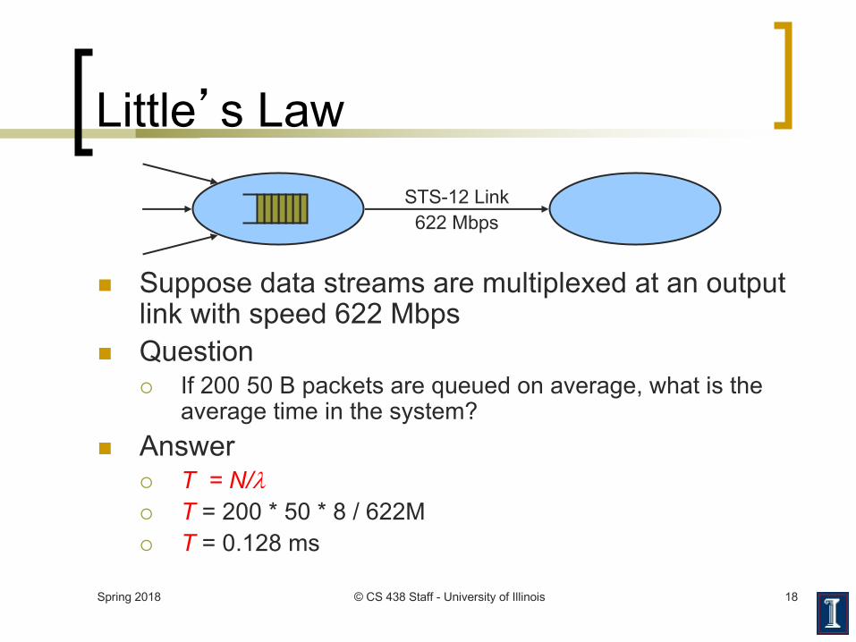
Little�s Law
n Suppose data streams are multiplexed at an output link with speed 622 Mbps
n Question¡ If 200 50 B packets are queued on average, what is the
average time in the system?
n Answer¡ T = N/l¡ T = 200 * 50 * 8 / 622M¡ T = 0.128 ms
STS-12 Link622 Mbps
Spring 2018 © CS 438 Staff - University of Illinois 19
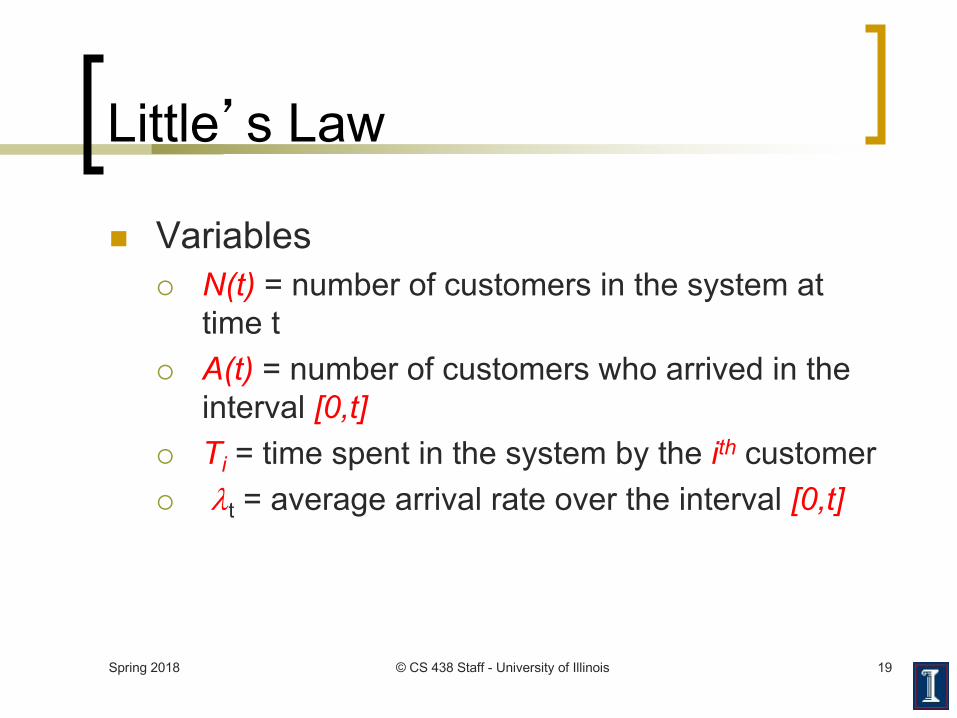
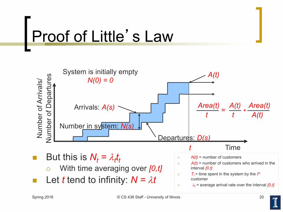
Little�s Law
n Variables¡ N(t) = number of customers in the system at
time t¡ A(t) = number of customers who arrived in the
interval [0,t]¡ Ti = time spent in the system by the ith customer¡ lt = average arrival rate over the interval [0,t]
Spring 2018 © CS 438 Staff - University of Illinois 20
Proof of Little�s Law
n But this is Nt = lttt¡ With time averaging over [0,t]
n Let t tend to infinity: N = lt
Arrivals: A(s)
Departures: D(s)
System is initially empty N(0) = 0
A(t)
t
Number in system: N(s)
Area(t)t
A(t)t
Area(t)A(t)
= *
Num
ber o
f Arri
vals
/N
umbe
r of D
epar
ture
s
Time¡ N(t) = number of customers¡ A(t) = number of customers who arrived in the
interval [0,t]¡ Ti = time spent in the system by the ith
customer¡ lt = average arrival rate over the interval [0,t]
Spring 2018 © CS 438 Staff - University of Illinois 21
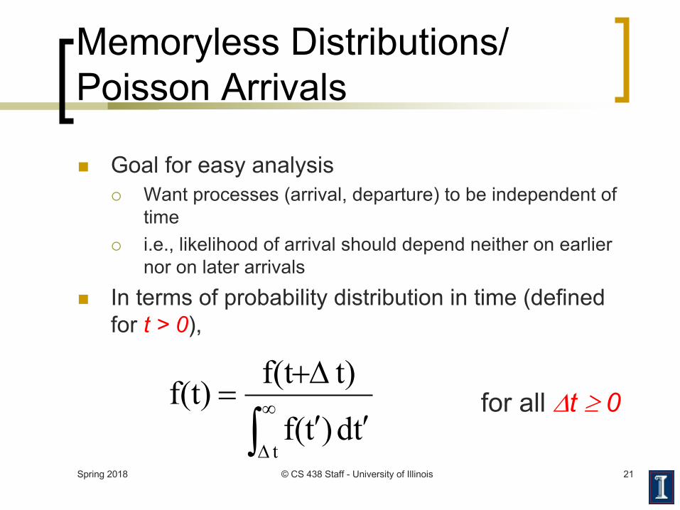
Memoryless Distributions/
Poisson Arrivals
n Goal for easy analysis
¡ Want processes (arrival, departure) to be independent of
time
¡ i.e., likelihood of arrival should depend neither on earlier
nor on later arrivals
n In terms of probability distribution in time (defined
for t > 0),
ò¥
D¢¢
D+=
ttd)tf(
t)f(tf(t) for all Dt ³ 0
Spring 2018 © CS 438 Staff - University of Illinois 22
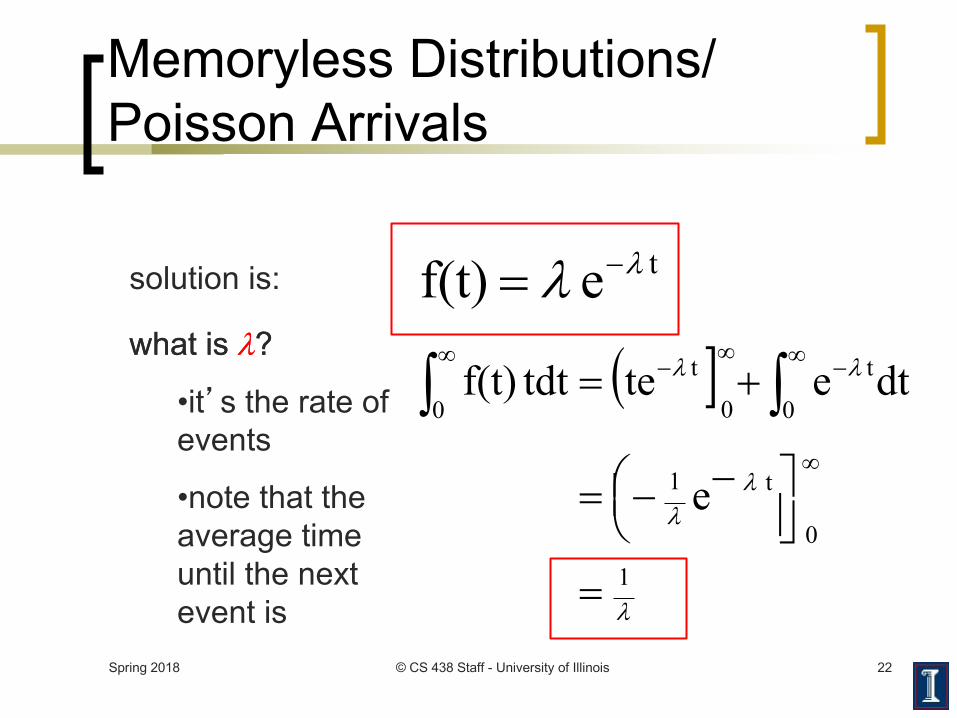
Memoryless Distributions/ Poisson Arrivals
solution is: tef(t) ll -=what is l?
•it�s the rate of events
•note that the average time until the next event is
( ]
l
ll
ll
1
0
t1
0
t
0
t
0
e
dtetetdtf(t)
=
úûùç
èæ --=
+=
¥
¥ -¥
-¥
òòwhat is l?
Spring 2018 © CS 438 Staff - University of Illinois 23
Plan
n Review exponential and Poisson probability distributions
n Discuss Poisson point processes and the M/M/1 queue model
Spring 2018 © CS 438 Staff - University of Illinois 24
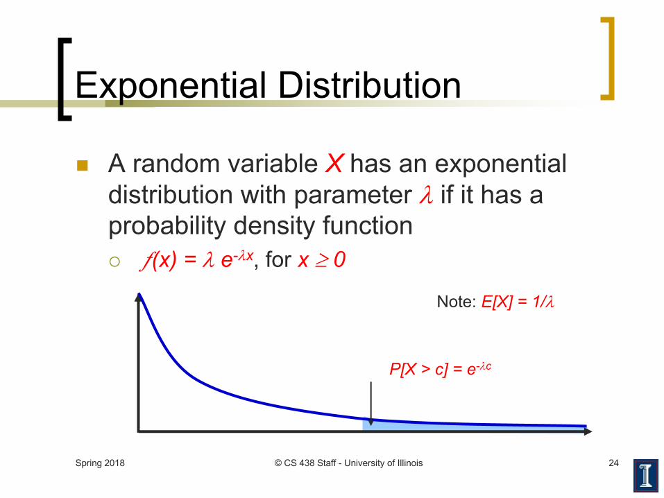
Exponential Distribution
n A random variable X has an exponential distribution with parameter l if it has a probability density function¡ ƒ(x) = l e-lx, for x ³ 0
P[X > c] = e-lc
Note: E[X] = 1/l
Spring 2018 © CS 438 Staff - University of Illinois 25
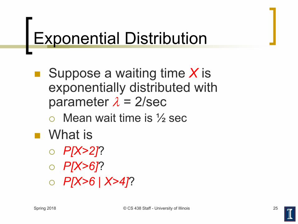
Exponential Distribution
n Suppose a waiting time X is exponentially distributed with parameter l = 2/sec¡ Mean wait time is ½ sec
n What is¡ P[X>2]?¡ P[X>6]?¡ P[X>6 | X>4]?
Spring 2018 © CS 438 Staff - University of Illinois 26
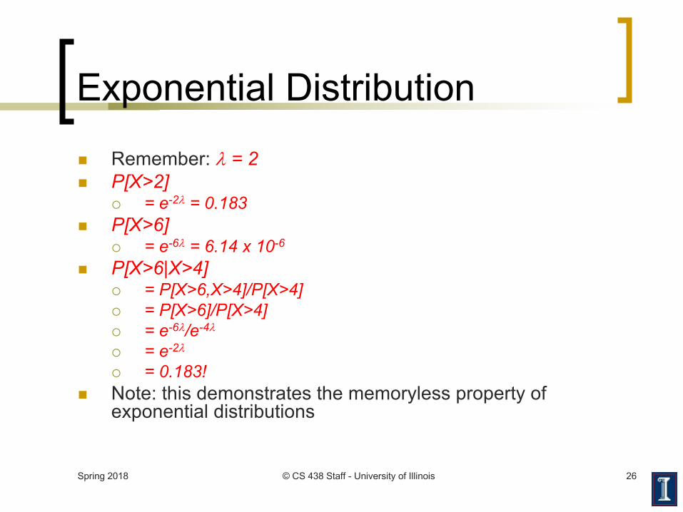
Exponential Distributionn Remember: l = 2n P[X>2]
¡ = e-2l = 0.183n P[X>6]
¡ = e-6l = 6.14 x 10⁻⁶
n P[X>6|X>4]¡ = P[X>6,X>4]/P[X>4]¡ = P[X>6]/P[X>4]¡ = e-6l/e-4l
¡ = e-2l
¡ = 0.183!n Note: this demonstrates the memoryless property of
exponential distributions
Spring 2018 © CS 438 Staff - University of Illinois 27
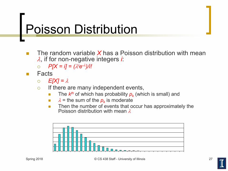
Poisson Distribution
n The random variable X has a Poisson distribution with mean l, if for non-negative integers i:¡ P[X = i] = (lie-l)/i!
n Facts¡ E[X] = l¡ If there are many independent events,
n The kth of which has probability pk (which is small) andn l = the sum of the pk is moderaten Then the number of events that occur has approximately the
Poisson distribution with mean l
Spring 2018 © CS 438 Staff - University of Illinois 28
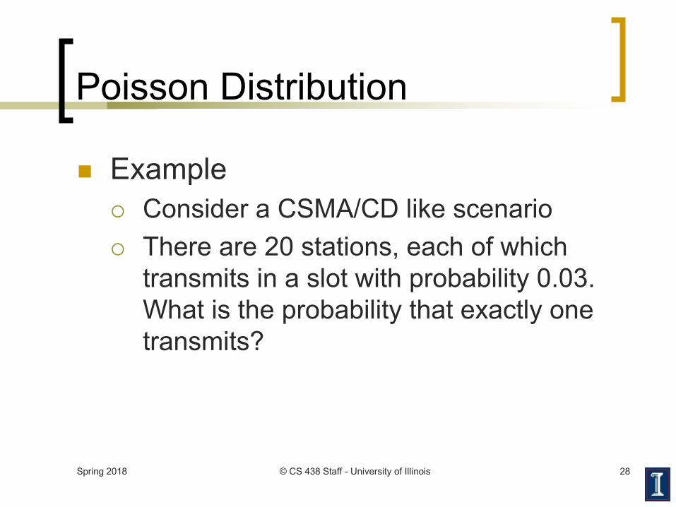
Poisson Distribution
n Example¡ Consider a CSMA/CD like scenario¡ There are 20 stations, each of which
transmits in a slot with probability 0.03. What is the probability that exactly one transmits?
Spring 2018 © CS 438 Staff - University of Illinois 29
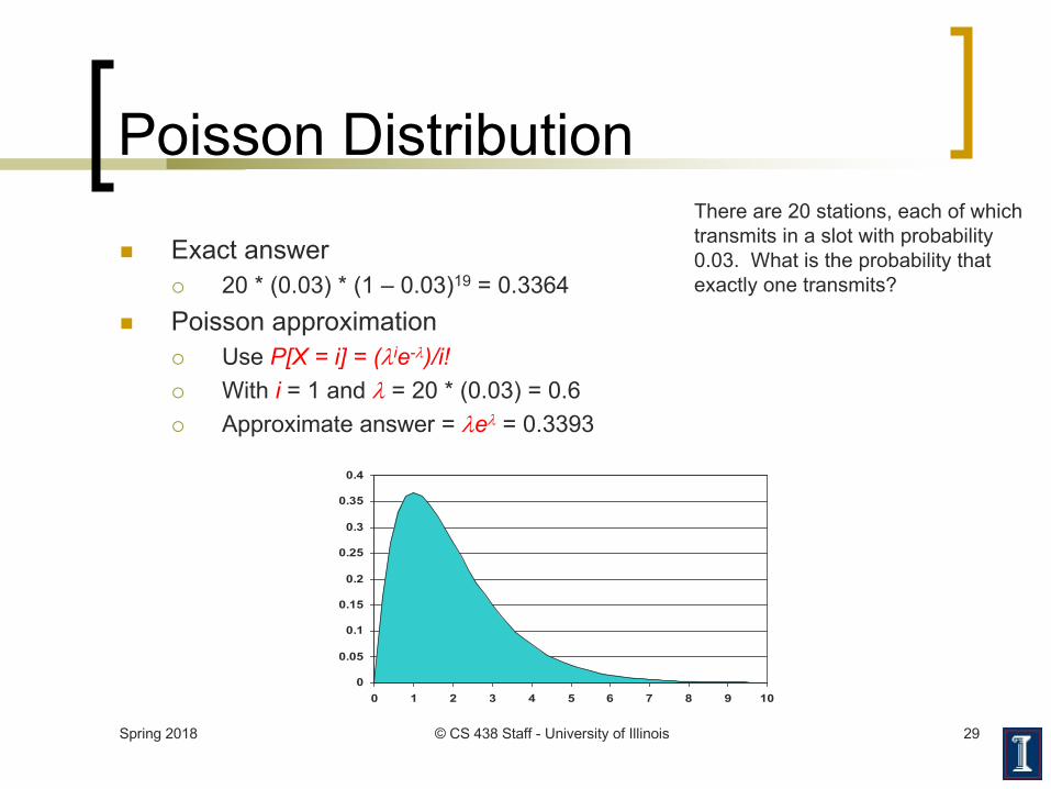
Poisson Distribution
n Exact answer¡ 20 * (0.03) * (1 – 0.03)19 = 0.3364
n Poisson approximation¡ Use P[X = i] = (lie-l)/i!¡ With i = 1 and l = 20 * (0.03) = 0.6¡ Approximate answer = lel = 0.3393
0
0.05
0.1
0.15
0.2
0.25
0.3
0.35
0.4
0 1 2 3 4 5 6 7 8 9 10
There are 20 stations, each of which transmits in a slot with probability 0.03. What is the probability that exactly one transmits?
Spring 2018 © CS 438 Staff - University of Illinois 30
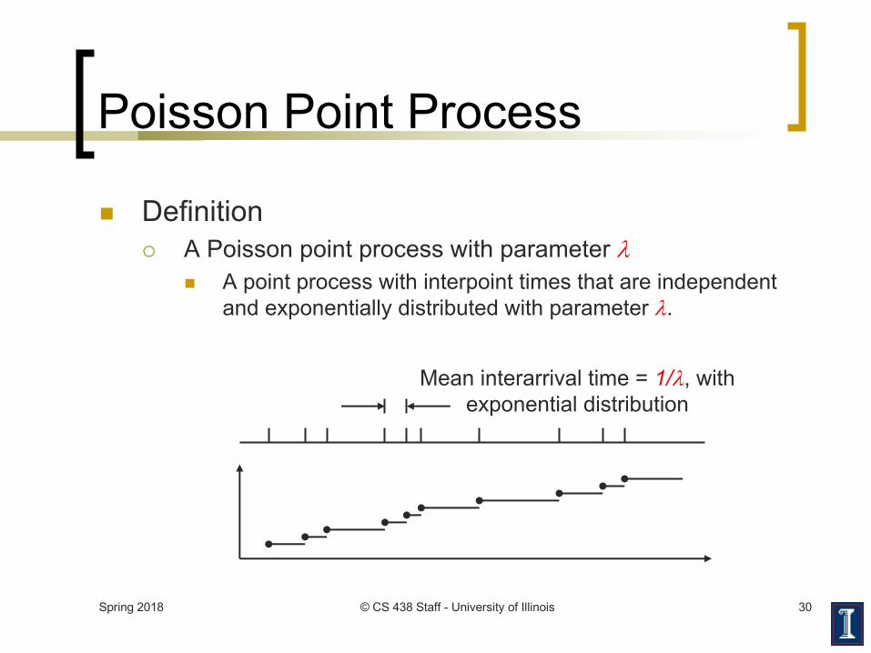
Poisson Point Process
n Definition¡ A Poisson point process with parameter l
n A point process with interpoint times that are independent and exponentially distributed with parameter l.
Mean interarrival time = 1/l, with exponential distribution
Spring 2018 © CS 438 Staff - University of Illinois 31
Poisson Point Process
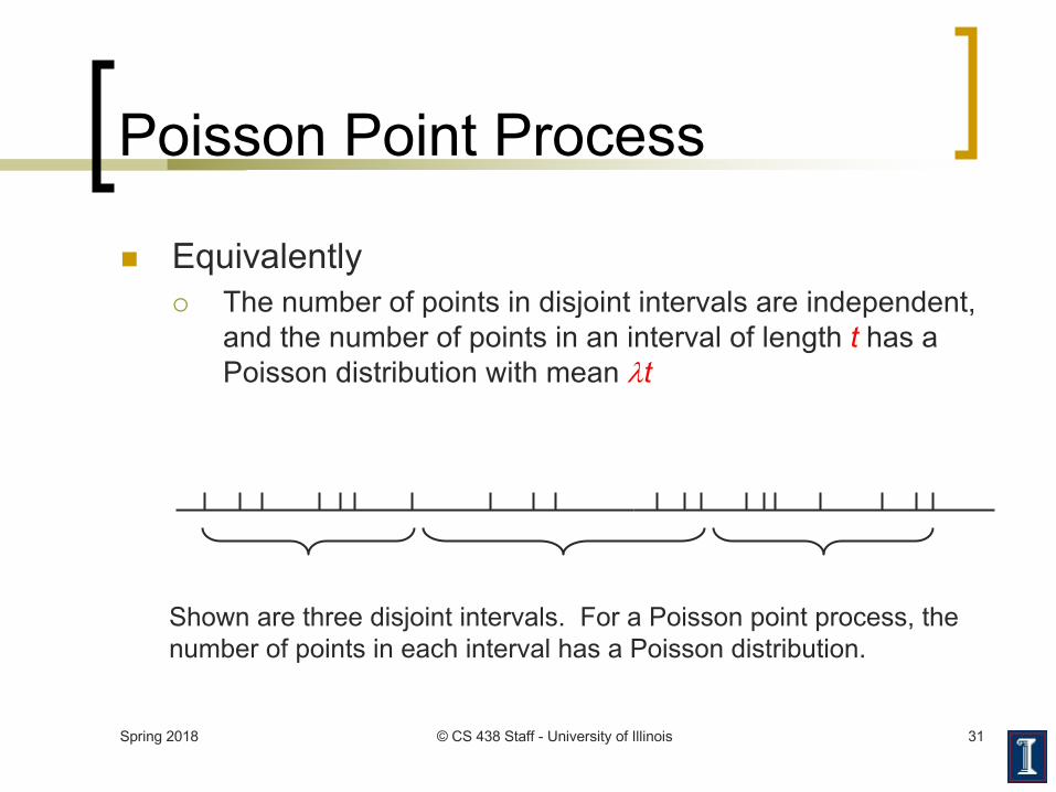
n Equivalently¡ The number of points in disjoint intervals are independent,
and the number of points in an interval of length t has a Poisson distribution with mean lt
Shown are three disjoint intervals. For a Poisson point process, the number of points in each interval has a Poisson distribution.
Spring 2018 © CS 438 Staff - University of Illinois 32
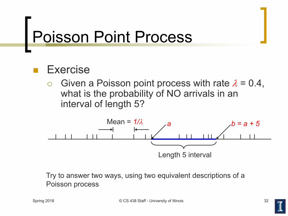
Poisson Point Process
n Exercise¡ Given a Poisson point process with rate l = 0.4,
what is the probability of NO arrivals in an interval of length 5?
Try to answer two ways, using two equivalent descriptions of a Poisson process
Mean = 1/l
Length 5 interval
a b = a + 5
Spring 2018 © CS 438 Staff - University of Illinois 33
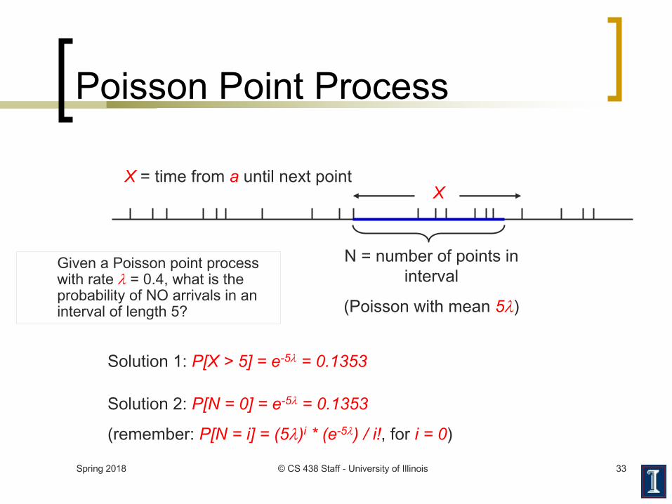
Poisson Point Process
Solution 1: P[X > 5] = e-5l = 0.1353
N = number of points in interval
(Poisson with mean 5l)
X = time from a until next pointX
Solution 2: P[N = 0] = e-5l = 0.1353
(remember: P[N = i] = (5l)i * (e-5l) / i!, for i = 0)
Given a Poisson point process with rate l = 0.4, what is the probability of NO arrivals in an interval of length 5?
Spring 2018 © CS 438 Staff - University of Illinois 34
Simple Queueing Systems
n Classify by ¡ �arrival pattern/service pattern/number of
servers�n Interarrival time probability density functionn The service time probability density functionn The number of serversn The queueing systemn The amount of buffer space in the queues
¡ Assumptionsn Infinite number of customers
Spring 2018 © CS 438 Staff - University of Illinois 35
Simple Queueing Systems
n Terminology¡ M = Markov (exponential probability density)¡ D = deterministic (all have same value)¡ G = general (arbitrary probability density)
n Example¡ M/D/4
n Markov arrival processn Deterministic service timesn 4 servers
Spring 2018 © CS 438 Staff - University of Illinois 36
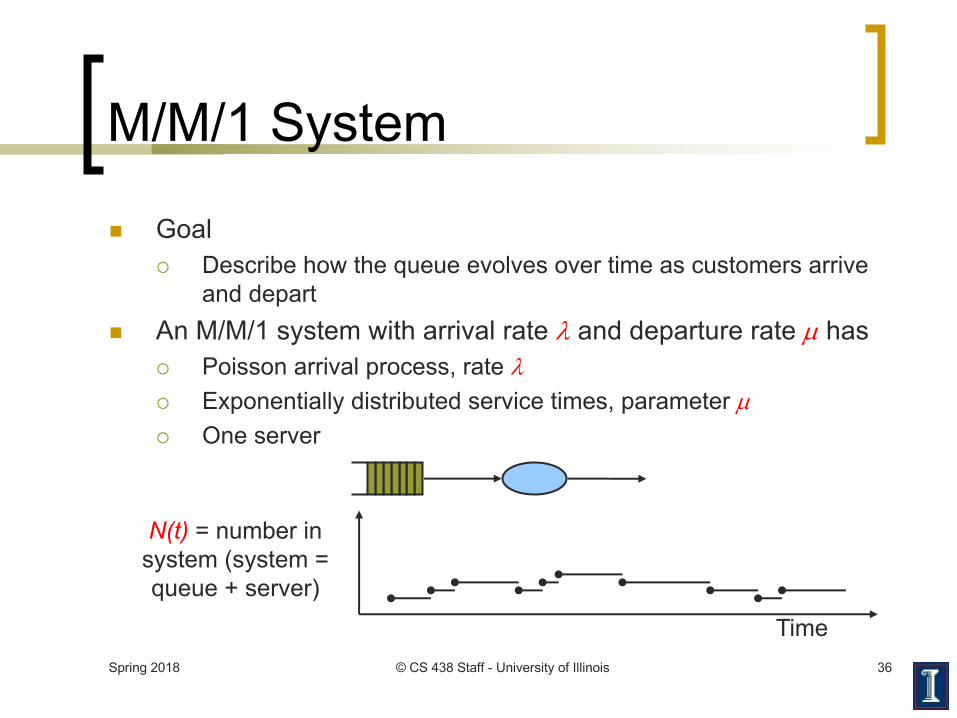
M/M/1 System
n Goal¡ Describe how the queue evolves over time as customers arrive
and depart
n An M/M/1 system with arrival rate l and departure rate µ has¡ Poisson arrival process, rate l¡ Exponentially distributed service times, parameter µ¡ One server
N(t) = number in system (system = queue + server)
Time
Spring 2018 © CS 438 Staff - University of Illinois 37
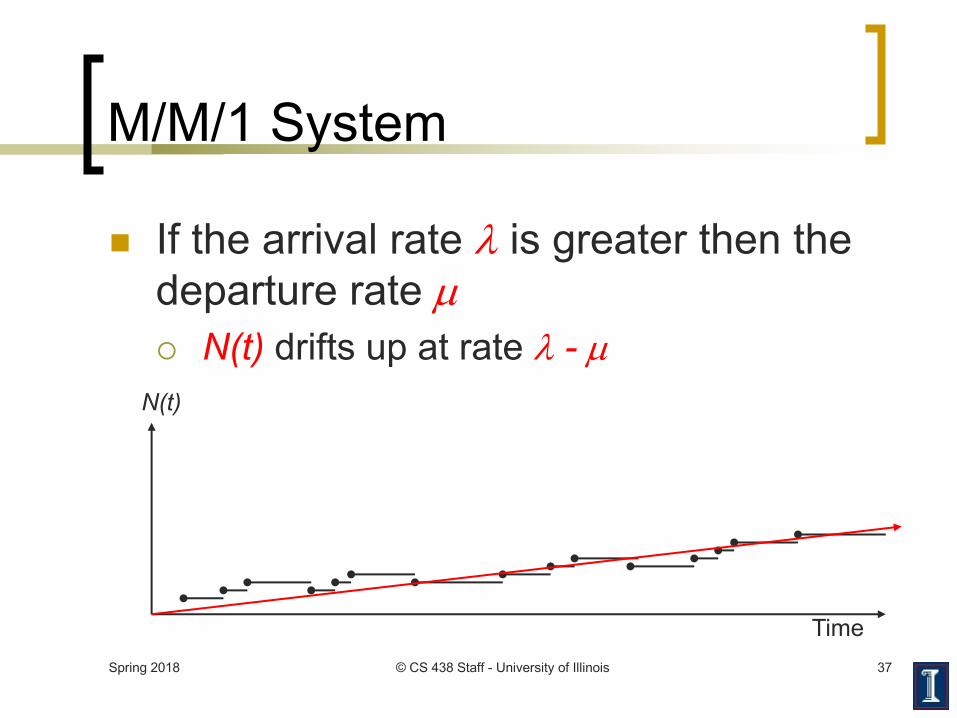
M/M/1 System
n If the arrival rate l is greater then the departure rate µ¡ N(t) drifts up at rate l - µN(t)
Time
Spring 2018 © CS 438 Staff - University of Illinois 38
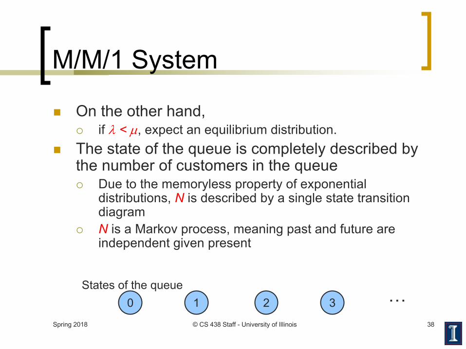
M/M/1 System
n On the other hand,
¡ if l < µ, expect an equilibrium distribution.
n The state of the queue is completely described by
the number of customers in the queue
¡ Due to the memoryless property of exponential
distributions, N is described by a single state transition
diagram
¡ N is a Markov process, meaning past and future are
independent given present
0 1 2 3…
States of the queue
Spring 2018 © CS 438 Staff - University of Illinois 39
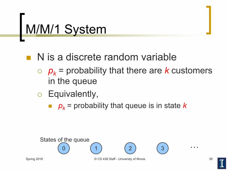
M/M/1 System
n N is a discrete random variable¡ pk = probability that there are k customers
in the queue¡ Equivalently,
n pk = probability that queue is in state k
0 1 2 3 …States of the queue
Spring 2018 © CS 438 Staff - University of Illinois 40
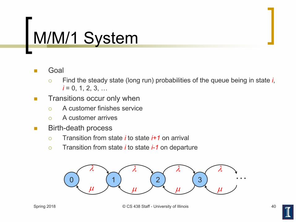
M/M/1 System
n Goal
¡ Find the steady state (long run) probabilities of the queue being in state i, i = 0, 1, 2, 3, …
n Transitions occur only when
¡ A customer finishes service
¡ A customer arrives
n Birth-death process
¡ Transition from state i to state i+1 on arrival
¡ Transition from state i to state i-1 on departure
0 1 2 3
l l l l
µ µ µ µ…
Spring 2018 © CS 438 Staff - University of Illinois 41
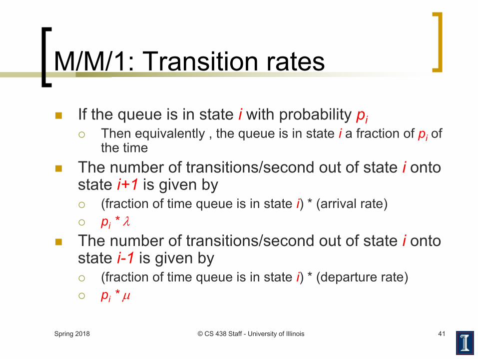
M/M/1: Transition rates
n If the queue is in state i with probability pi¡ Then equivalently , the queue is in state i a fraction of pi of
the timen The number of transitions/second out of state i onto
state i+1 is given by¡ (fraction of time queue is in state i) * (arrival rate)¡ pi * l
n The number of transitions/second out of state i onto state i-1 is given by¡ (fraction of time queue is in state i) * (departure rate)¡ pi * µ
Spring 2018 © CS 438 Staff - University of Illinois 42
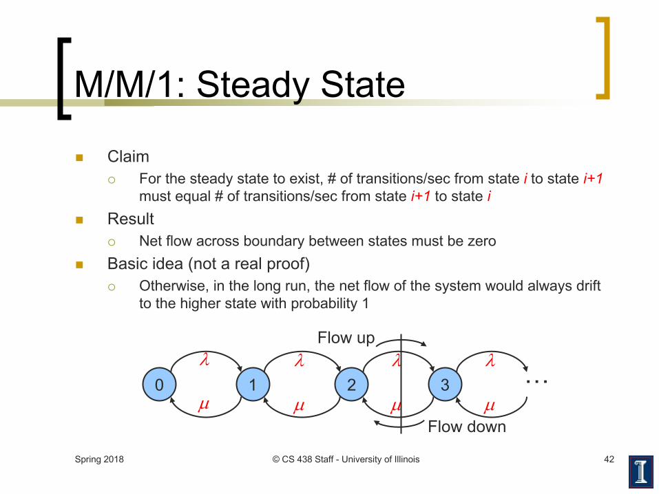
M/M/1: Steady State
n Claim¡ For the steady state to exist, # of transitions/sec from state i to state i+1
must equal # of transitions/sec from state i+1 to state in Result
¡ Net flow across boundary between states must be zero
n Basic idea (not a real proof)¡ Otherwise, in the long run, the net flow of the system would always drift
to the higher state with probability 1
0 1 2 3l l l l
µ µ µ µ…
Flow up
Flow down
Spring 2018 © CS 438 Staff - University of Illinois 43
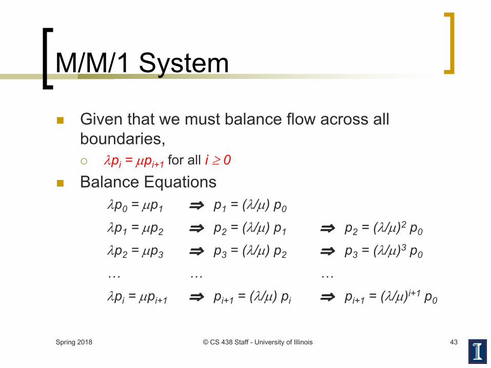
M/M/1 System
n Given that we must balance flow across all boundaries,¡ lpi = µpi+1 for all i ³ 0
n Balance Equationslp0 = µp1
lp1 = µp2
lp2 = µp3
…
lpi = µpi+1
Þ p1 = (l/µ) p0
Þ p2 = (l/µ) p1
Þ p3 = (l/µ) p2
…
Þ pi+1 = (l/µ) pi
Þ p2 = (l/µ)2 p0
Þ p3 = (l/µ)3 p0
…
Þ pi+1 = (l/µ)i+1 p0
Spring 2018 © CS 438 Staff - University of Illinois 44
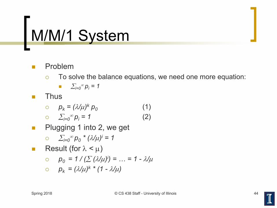
M/M/1 System
n Problem¡ To solve the balance equations, we need one more equation:
n åi=0¥ pi = 1
n Thus¡ pk = (l/µ)k p0 (1)¡ åi=0
¥ pi = 1 (2)n Plugging 1 into 2, we get
¡ åi=0¥ p0 * (l/µ)i = 1
n Result (for l < µ)¡ p0 = 1 / (å (l/µ)i) = … = 1 - l/µ¡ pk = (l/µ)k * (1 - l/µ)
Spring 2018 © CS 438 Staff - University of Illinois 45
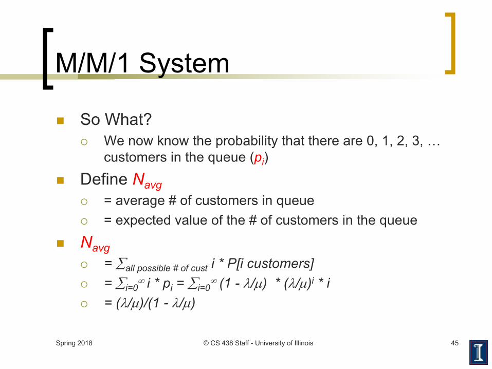
M/M/1 System
n So What?¡ We now know the probability that there are 0, 1, 2, 3, …
customers in the queue (pi)
n Define Navg¡ = average # of customers in queue¡ = expected value of the # of customers in the queue
n Navg¡ = åall possible # of cust i * P[i customers]¡ = åi=0
¥ i * pi = åi=0¥ (1 - l/µ) * (l/µ)i * i
¡ = (l/µ)/(1 - l/µ)
Spring 2018 © CS 438 Staff - University of Illinois 46
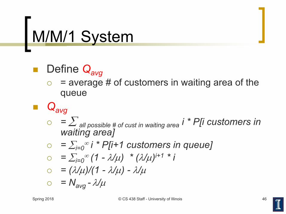
M/M/1 System
n Define Qavg¡ = average # of customers in waiting area of the
queuen Qavg
¡ = å all possible # of cust in waiting area i * P[i customers in waiting area]
¡ = åi=0¥ i * P[i+1 customers in queue]
¡ = åi=0¥ (1 - l/µ) * (l/µ)i+1 * i
¡ = (l/µ)/(1 - l/µ) - l/µ¡ = Navg - l/µ
Spring 2018 © CS 438 Staff - University of Illinois 47
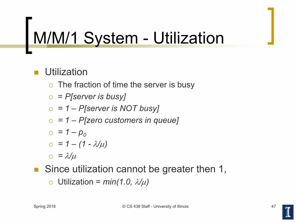
M/M/1 System - Utilization
n Utilization ¡ The fraction of time the server is busy¡ = P[server is busy]¡ = 1 – P[server is NOT busy]¡ = 1 – P[zero customers in queue]¡ = 1 – p0
¡ = 1 – (1 - l/µ)¡ = l/µ
n Since utilization cannot be greater then 1,¡ Utilization = min(1.0, l/µ)
Spring 2018 © CS 438 Staff - University of Illinois 48
M/M/1 System - Utilization
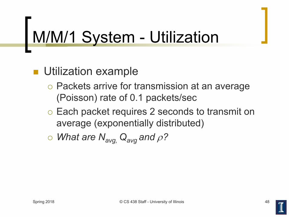
n Utilization example¡ Packets arrive for transmission at an average
(Poisson) rate of 0.1 packets/sec¡ Each packet requires 2 seconds to transmit on
average (exponentially distributed)¡ What are Navg, Qavg and r?
Spring 2018 © CS 438 Staff - University of Illinois 49
M/M/1 System - Utilization
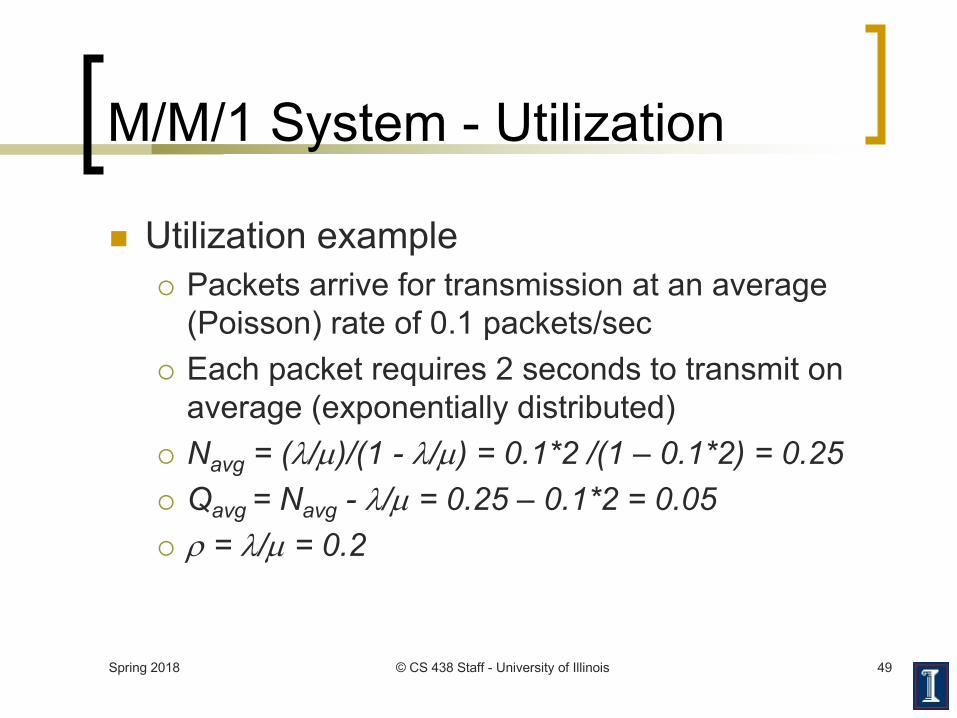
n Utilization example¡ Packets arrive for transmission at an average
(Poisson) rate of 0.1 packets/sec¡ Each packet requires 2 seconds to transmit on
average (exponentially distributed)¡ Navg = (l/µ)/(1 - l/µ) = 0.1*2 /(1 – 0.1*2) = 0.25¡ Qavg = Navg - l/µ = 0.25 – 0.1*2 = 0.05¡ r = l/µ = 0.2
Spring 2018 © CS 438 Staff - University of Illinois 50
M/M/1 System - Utilization
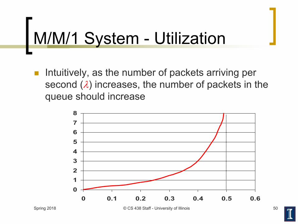
n Intuitively, as the number of packets arriving per second (l) increases, the number of packets in the queue should increase
012345678
0 0.1 0.2 0.3 0.4 0.5 0.6
Spring 2018 © CS 438 Staff - University of Illinois 51
M/M/1 System - Utilization
n Normalized Traffic Parameter (r)¡ Note that Navg and Qavg only depend on the ratio l/µ¡ Define r
n = (avg arrival rate * avg service time)n = l * 1/µ = l/µ
¡ Intuitively, if we scale both arrival rate and service time by a constant factor, Navg and Qavg should remain the same
¡ Noten If l > µ (i.e. l/µ > 1), then more packets are arriving per
second than can be servicedn Thus, Navg and Qavg are unbounded when r ³ 1!
Spring 2018 © CS 438 Staff - University of Illinois 52
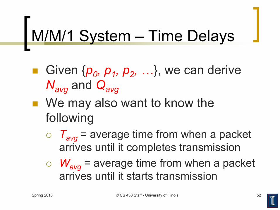
M/M/1 System – Time Delays
n Given {p0, p1, p2, …}, we can derive Navg and Qavg
n We may also want to know the following¡ Tavg = average time from when a packet
arrives until it completes transmission¡ Wavg = average time from when a packet
arrives until it starts transmission
Spring 2018 © CS 438 Staff - University of Illinois 53
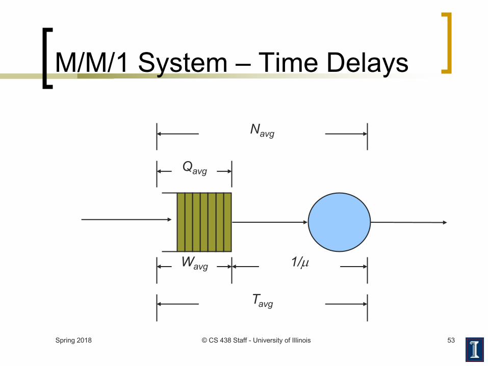
M/M/1 System – Time Delays
Qavg
Navg
Wavg
Tavg
1/µ
Spring 2018 © CS 438 Staff - University of Illinois 54
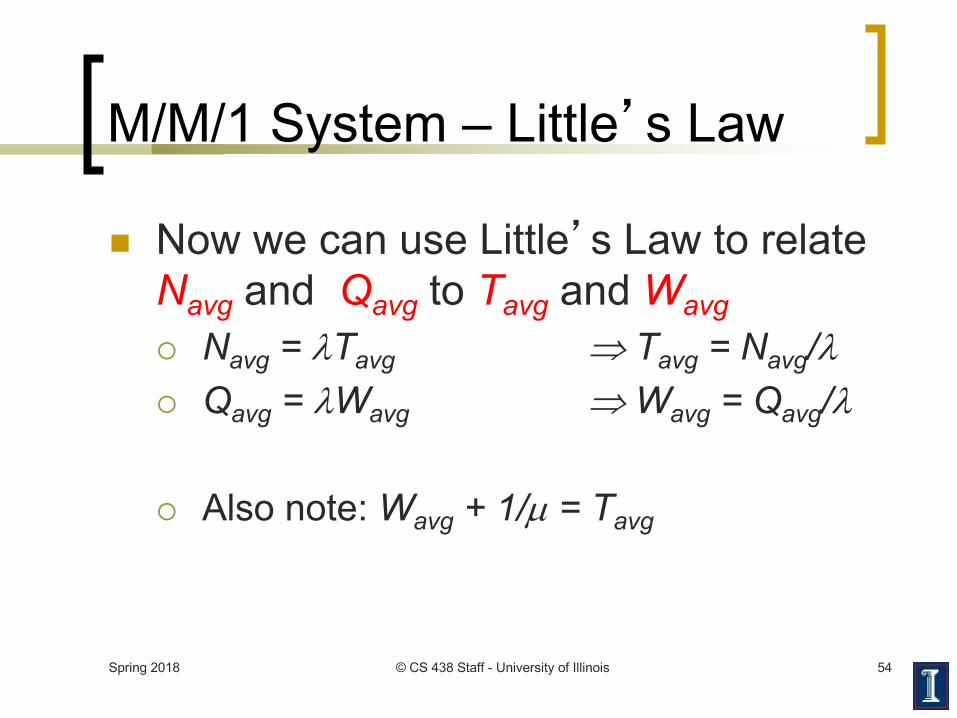
M/M/1 System – Little�s Law
n Now we can use Little�s Law to relate Navg and Qavg to Tavg and Wavg ¡ Navg = lTavg Þ Tavg = Navg/l¡ Qavg = lWavg Þ Wavg = Qavg/l
¡ Also note: Wavg + 1/µ = Tavg
Spring 2018 © CS 438 Staff - University of Illinois 55
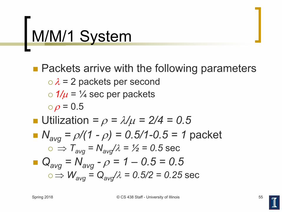
M/M/1 System
n Packets arrive with the following parameters
¡ l = 2 packets per second
¡ 1/µ = ¼ sec per packets
¡ r = 0.5
n Utilization = r = l/µ = 2/4 = 0.5n Navg = r/(1 - r) = 0.5/1-0.5 = 1 packet
¡ Þ Tavg = Navg/l = ½ = 0.5 sec
n Qavg = Navg - r = 1 – 0.5 = 0.5¡Þ Wavg = Qavg/l = 0.5/2 = 0.25 sec
Spring 2018 © CS 438 Staff - University of Illinois 56
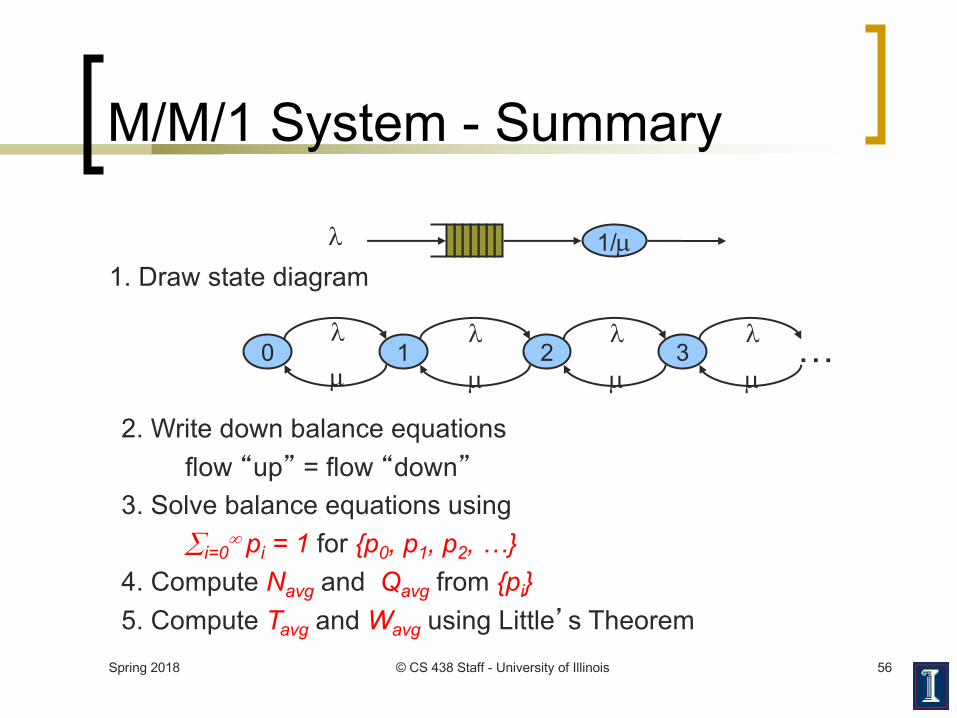
M/M/1 System - Summary
1. Draw state diagram1/µl
0 1 2 3l l l l
µ µ µ µ…
2. Write down balance equationsflow �up� = flow �down�
3. Solve balance equations using åi=0
¥ pi = 1 for {p0, p1, p2, …}4. Compute Navg and Qavg from {pi} 5. Compute Tavg and Wavg using Little�s Theorem
Spring 2018 © CS 438 Staff - University of Illinois 57
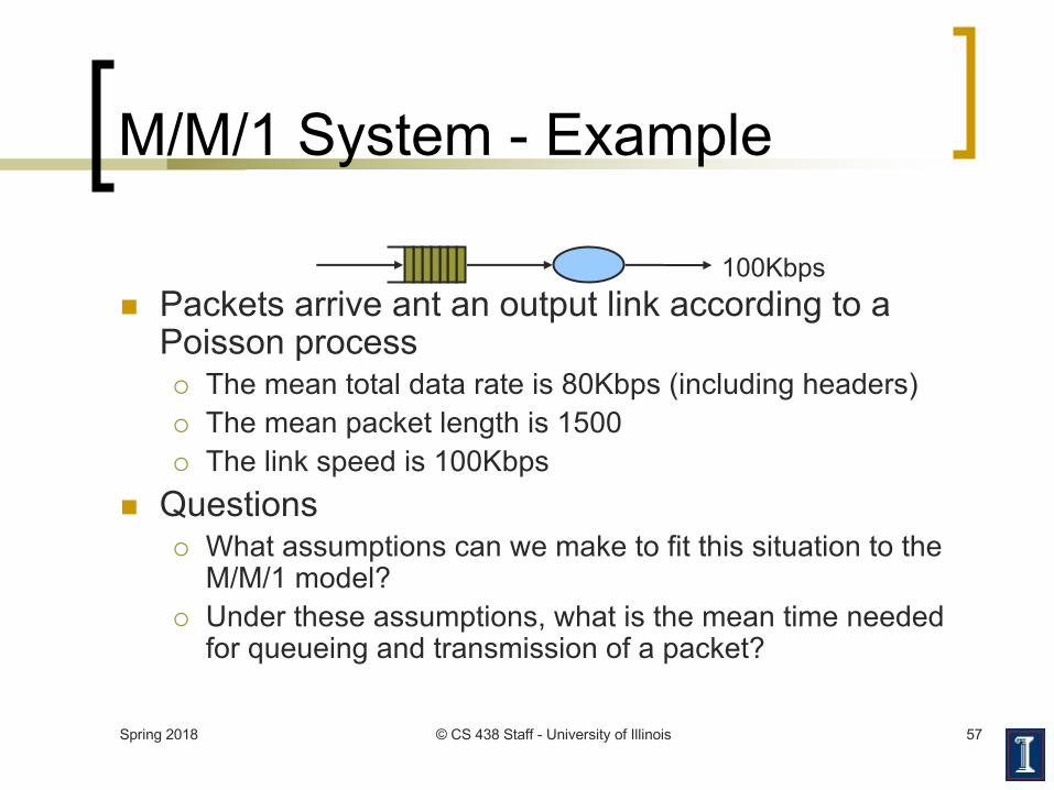
M/M/1 System - Example
n Packets arrive ant an output link according to a Poisson process¡ The mean total data rate is 80Kbps (including headers)¡ The mean packet length is 1500¡ The link speed is 100Kbps
n Questions ¡ What assumptions can we make to fit this situation to the
M/M/1 model?¡ Under these assumptions, what is the mean time needed
for queueing and transmission of a packet?
100Kbps
Spring 2018 © CS 438 Staff - University of Illinois 58
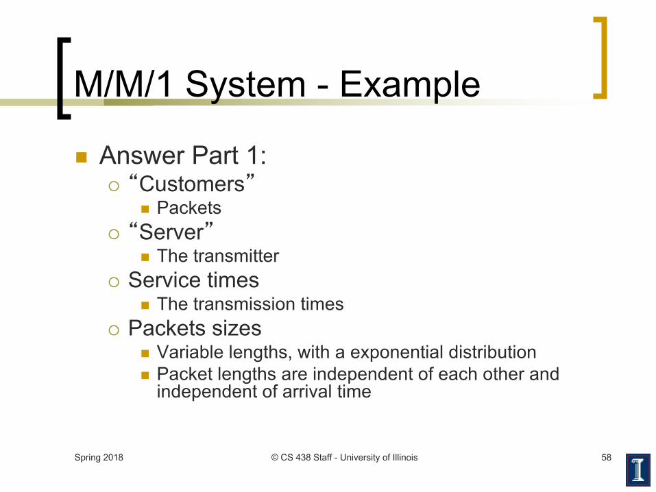
M/M/1 System - Example
n Answer Part 1:¡ �Customers�
n Packets¡ �Server�
n The transmitter¡ Service times
n The transmission times¡ Packets sizes
n Variable lengths, with a exponential distributionn Packet lengths are independent of each other and
independent of arrival time
Spring 2018 © CS 438 Staff - University of Illinois 59
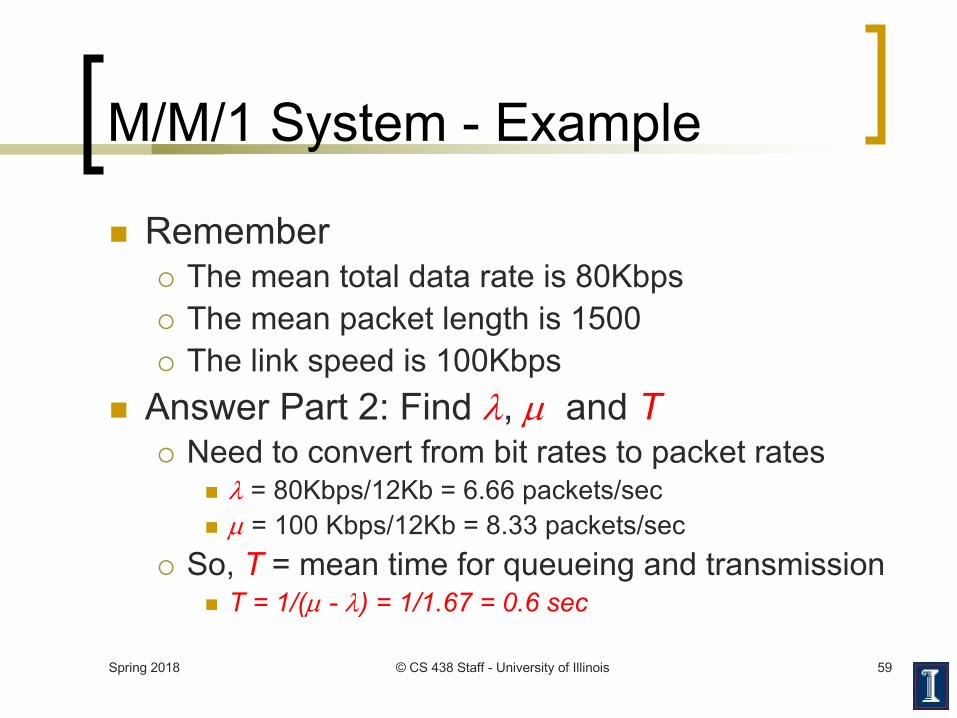
M/M/1 System - Example
n Remember¡ The mean total data rate is 80Kbps ¡ The mean packet length is 1500¡ The link speed is 100Kbps
n Answer Part 2: Find l, µ and T¡ Need to convert from bit rates to packet rates
n l = 80Kbps/12Kb = 6.66 packets/secn µ = 100 Kbps/12Kb = 8.33 packets/sec
¡ So, T = mean time for queueing and transmissionn T = 1/(µ - l) = 1/1.67 = 0.6 sec
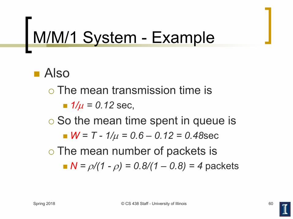
M/M/1 System - Example
n Also¡ The mean transmission time is
n 1/µ = 0.12 sec,
¡ So the mean time spent in queue is n W = T - 1/µ = 0.6 – 0.12 = 0.48sec
¡ The mean number of packets is n N = r/(1 - r) = 0.8/(1 – 0.8) = 4 packets
Spring 2018 © CS 438 Staff - University of Illinois 60
Spring 2018 © CS 438 Staff - University of Illinois 61
M/M/1 System in Practice
n The assumptions we made are often not realisticn We still get the correct qualitative behaviorn Simple formulas for predictive delay are useful for
provisioning resources in a network and setting controls
n Real traffic seems to have bursty behavior on multiple time scales¡ This is not true for Poisson processes