Embed Size (px)
Citation preview
Methods for the specification and verification of business processes
MPB (6 cfu, 295AA)
Roberto Bruni http://www.di.unipi.it/~bruni
19 - Diagnosis for WF nets
1
Object
2
We study suitable diagnosis techniques for unsound Workflow nets
Diagnosing workflow processes using Woflan (article, optional reading) http://wwwis.win.tue.nl/~wvdaalst/publications/p135.pdf
Some Pragmatic Considerations
3
We know that, for free-choice nets, liveness and boundedness can be decided efficiently
(in polynomial time)
but we want to check soundness for a wider range of nets
Moreover, when a process is not sound, some diagnostic can be generated that indicates why it is flawed
Woflan (now a ProM plugin)
4
WOrkFLow ANalyzer (Windows only) http://www.win.tue.nl/woflan/
Woflan tells us if N is a sound workflow net (Is N a workflow net? Is N* bounded? Is N* live?)
if not, provides some diagnostic information
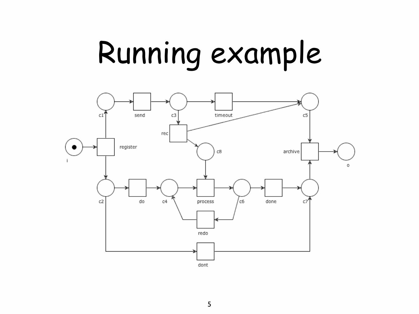
Running example
5
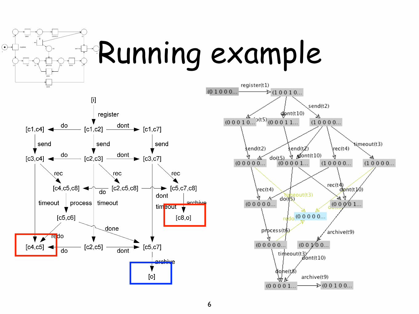
Running example
6
6 H. VERBEEK, T. BASTEN AND W. VAN DER AALST
FIGURE 6. S-components of net N
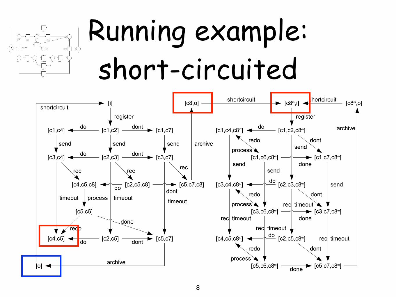
2.2.3. Occurrence graph
The set of occurrence sequences of a system can be embed-
ded into a graph. Every occurrence sequence corresponds to
some path in that graph and vice versa.
NOTATION 2.2. (Reachability) Let N = (P, T, F) be
a P/T net. Marking M1 is reachable from marking M0, de-
noted M0 �⇧ M1, iff system (N ,M0) has an occurrence
sequence ending in M1.
In system S of Figure 2, marking [c4,c5,c8] is reachable
from the initial marking [i], while from [c4,c5,c8] both
[c4,c5] and [o] are reachable.
DEFINITION 2.15. (Occurrence graph) Let S = ((P, T,
F),M0) be a system; let H ⌅ B(P) be a set of markings,
let A ⌅ (H ⇥ T ⇥ H) be a set of T -labeled arcs, and let
G = (H, A) be a graph which satisfies the following re-
quirements:
(i). H = {M ⌃ B(P)|M0 �⇧ M};(ii). A = {(M, t,M1) ⌃ (H ⇥ T ⇥ H)|M t�⇧ M1}.
Graph G is called the occurrence (or reachability) graph
(OG) of S.
The OG of system S of Figure 2 is given in Figure 7.
The OG embeds precisely all occurrence sequences of the
system. The construction of this graph is straightforward,
although termination is not guaranteed, because it might
be infinite. For example, the OG of system S of Figure 3
has infinitely many nodes. In this system, firing the tran-
sitions register send rec dont archive short-
circuit over and over again, leads to infinitely many
markings [i,c8n], for arbitrary n > 0. After one firing of
these transitions, there is one token in c8, after two firings
there are two, and so on. There is no limit to the number of
tokens in c8. Place c8 is said to be unbounded. As a result,
the number of markings in the OG is infinite.
FIGURE 7. The OG of system S
2.2.4. Coverability graph
A solution to cope with unbounded places is the notion of a
so-called coverability graph. A coverability graph is a finite
variant of an OG. However, we have to pay a price: First, we
must allow markings to be infinite to deal with unbounded
behavior. Second, a P/T system may have a number of pos-
sible coverability graphs, whereas it always has one unique
OG.
An extended bag over some alphabet A is a function from
A to the natural numbers plus � (denoting infinity). The set
of all extended bags over A is denoted B�(A). All opera-
tions on bags can be defined for extended bags in a straight-
forward way. An extended bag M ⌃ B�(P) is called an
extended marking of a P/T net (P, T, F). The set of ex-
tended markings can be partitioned into a set of finite mark-
ings B(P) and a set of infinite markings B�(P) \ B(P).
A coverability graph of a system is a variant of the OG,
where paths in the OG with infinitely many different (fi-
nite) markings are represented by a finite number of infinite
markings. An infinite marking is introduced in a coverabil-
ity graph if we encounter a marking M1 on an occurrence
sequence that has a smaller marking M0 as one of its pre-
decessors: The places in M1 � M0 are unbounded and are
marked with �. It is known that a coverability graph is al-
ways finite ([33], p. 70).
DEFINITION 2.16. (Coverability graph) Let S = ((P, T,
F),M0) be a system, let H ⌅ B�(P) be a set of extended
markings, let A ⌅ (H ⇥ T ⇥ H) be a set of T -labeled arcs,
and let G = (H, A) be a graph which can be constructed as
follows:
(i). Initially, H = {M0} and A = ⌥.(ii). Take an M from H and a t from T such that M
enables t and such that no M1 exists with (M, t,M1) ⌃A. Let M2 = M�•t+t•. Add M3 to H and (M, t,M3)
to A, where for every p ⌃ P:
THE COMPUTER JOURNAL, Vol. ??, No. ??, ????
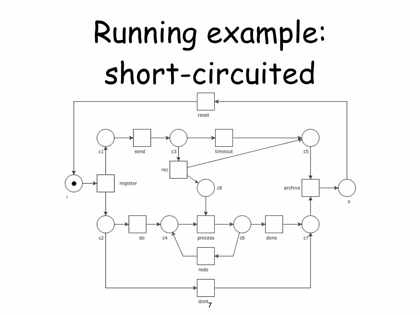
Running example: short-circuited
7
8 H. VERBEEK, T. BASTEN AND W. VAN DER AALST
FIGURE 8. The CG for the short-circuited system S
workflow processes. Cases are often generated by an exter-
nal customer. However, it is also possible that a case is gen-
erated by another department within the same organization
(internal customer). A typical example of a process that is
not case-based, and hence not a workflow process, is a pro-
duction process such as the assembly of bicycles. The task
of putting a tire on a wheel is (generally) independent of the
specific bicycle for which the wheel will be used. Note that
the production of bicycles to order, i.e., procurement, pro-
duction, and assembly are driven by individual orders, can
be considered as a workflow process.
The goal of workflow management is to handle cases as
efficient and effective as possible. A workflow process is
designed to handle large numbers of similar cases. Handling
one customer complaint usually does not differ much from
handling another customer complaint. The basis of a work-
flow process is the workflow process definition. This process
definition specifies which tasks need to be executed in what
order. Alternative terms for workflow process definition are:
‘procedure’, ‘workflow schema’, ‘flow diagram’, and ‘rout-
ing definition’. Tasks are ordered by specifying for each task
the conditions that need to be fulfilled before it may be ex-
ecuted. In addition, it is specified which conditions are ful-
filled by executing a specific task. Thus, a partial ordering of
tasks is obtained. In a workflow process definition, standard
routing elements are used to describe sequential, alternative,
parallel, and iterative routing thus specifying the appropri-
ate route of a case. The workflow management coalition
(WfMC) has standardized a few basic building blocks for
constructing workflow process definitions [29]. A so-called
OR-split is used to specify a choice between several alter-
natives; an OR-join specifies that several alternatives in the
workflow process definition come together. An AND-split
and an AND-join can be used to specify the beginning and
the end of parallel branches in the workflow process defini-
tion. The routing decisions in OR-splits are often based on
data such as the age of a customer, the department responsi-
ble, or the contents of a letter from the customer.
Many cases can be handled by following the same work-
flow process definition. As a result, the same task has to
be executed for many cases. A task that needs to be exe-
cuted for a specific case is called a work item. An example
of a work item is the order to execute task ‘send refund form
to customer’ for case ‘complaint of customer Baker’. Most
work items need a resource in order to be executed. A re-
source is either a machine (e.g., a printer or a fax) or a per-
son (participant, worker, or employee). Besides a resource,
a work item often needs a trigger. A trigger specifies who
or what initiates the execution of a work item. Often, the
trigger for a work item is the resource that must execute the
work item. Other common triggers are external triggers and
time triggers. An example of an external trigger is an incom-
ing phone call of a customer; an example of a time trigger is
the expiration of a deadline. A work item that is being ex-
ecuted is called an activity. If we take a photograph of the
state of a workflow, we see cases, work items, and activities.
Work items link cases and tasks. Activities link cases, tasks,
triggers, and resources.
A thorough investigation of the business processes in a
company that results in a complete set of efficient and ef-
fective workflow processes is the basis of the successful in-
troduction of a workflow system. Formal (qualitative and
quantitative) verification can be a useful aid in obtaining the
desired effectiveness and efficiency.
3.2. Workflow perspectives and abstraction
In the previous subsection, we introduced the workflow con-
cepts used in the remainder of this paper. Workflow man-
agement has many aspects and typically involves many dis-
ciplines. The verification tool presented in this paper fo-
THE COMPUTER JOURNAL, Vol. ??, No. ??, ????
Running example: short-circuited
8
Structural analysis
9
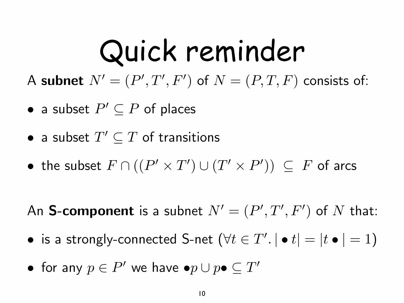
Quick reminder
10
A subnet N � = (P �, T �, F �) of N = (P, T, F ) consists of:
• a subset P � ⇥ P of places
• a subset T � ⇥ T of transitions
• the subset F ⌃ ((P � � T �) ⇧ (T � � P �)) ⇥ F of arcs
An S-component is a subnet N � = (P �, T �, F �) of N that:
• is a strongly-connected S-net (⌅t ⇤ T �. | • t| = |t • | = 1)
• for any p ⇤ P � we have •p ⇧ p• ⇥ T �
Quick reminder
11
In a S-component,the total number of tokens in its places is constant
Any S-componentinduces a uniform invariant (weights 0 and 1)
A net is S-coverable i�any p � P belongs to some S-component
S-coverability implies boundedness(because it induces a positive S-invariant)
S-Invariant analysis
12
If every place of N* is covered by a semi-positive S-invariant then N* is bounded
Places not covered by semi-positive S-invariants are potential sources of errors
S-Coverability vs Soundness
13
S-coverability is one of the basic requirements any workflow process definition should satisfy
Still: S-coverability is not a sufficient requirement for soundness
N* can be S-coverable even if N is not sound
N can be sound even if N* is not S-coverable
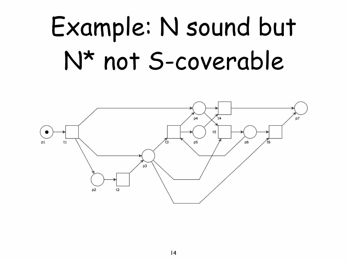
Example: N sound but N* not S-coverable
14
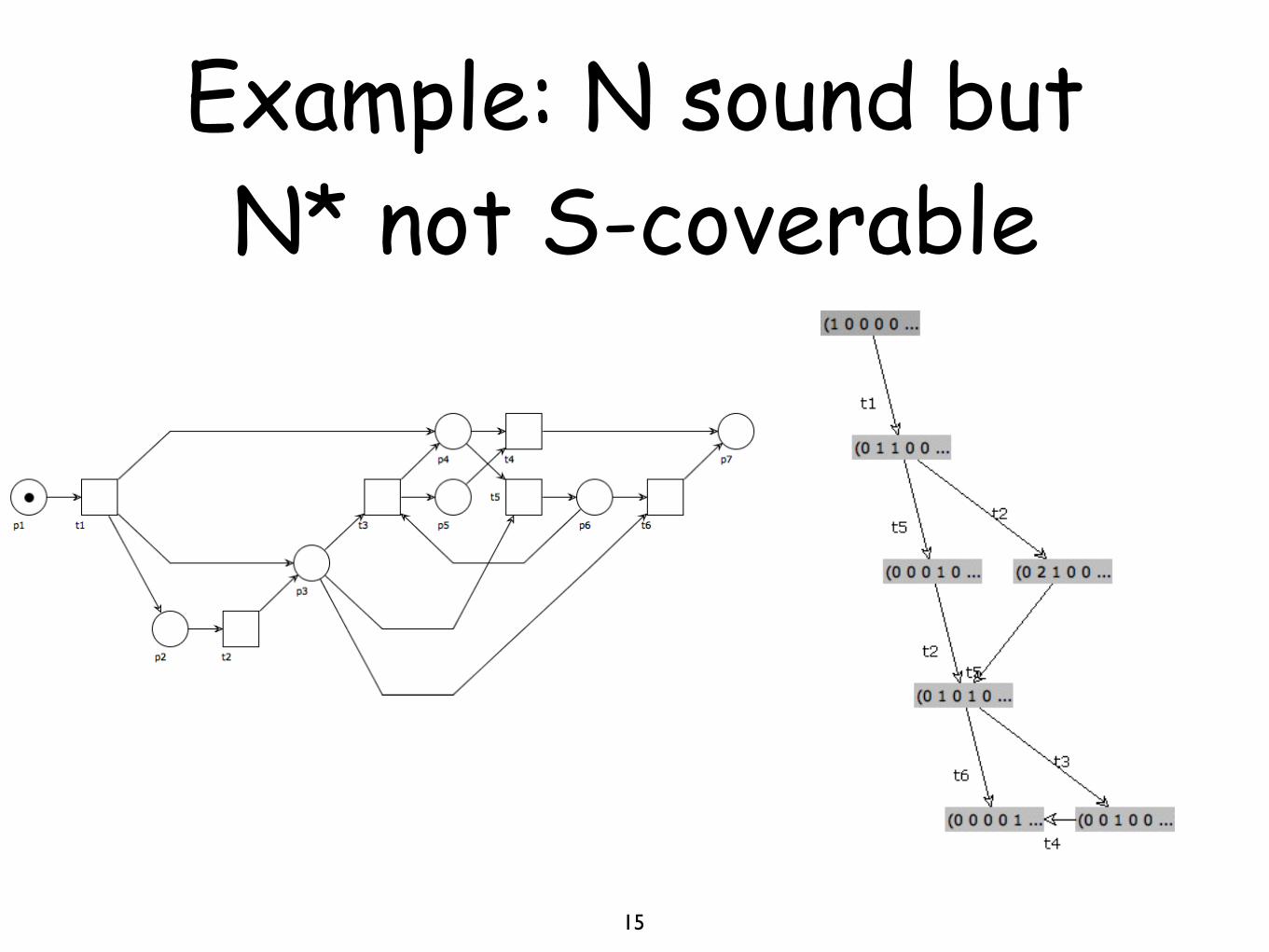
Example: N sound but N* not S-coverable
15
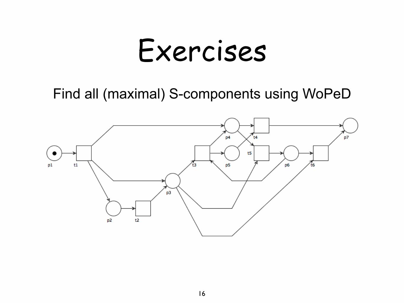
Exercises
16
Find all (maximal) S-components using WoPeD

Exercises
17
Draw a workflow net N that is S-coverable but such that N* is not sound

S-Coverability diagnosis
18
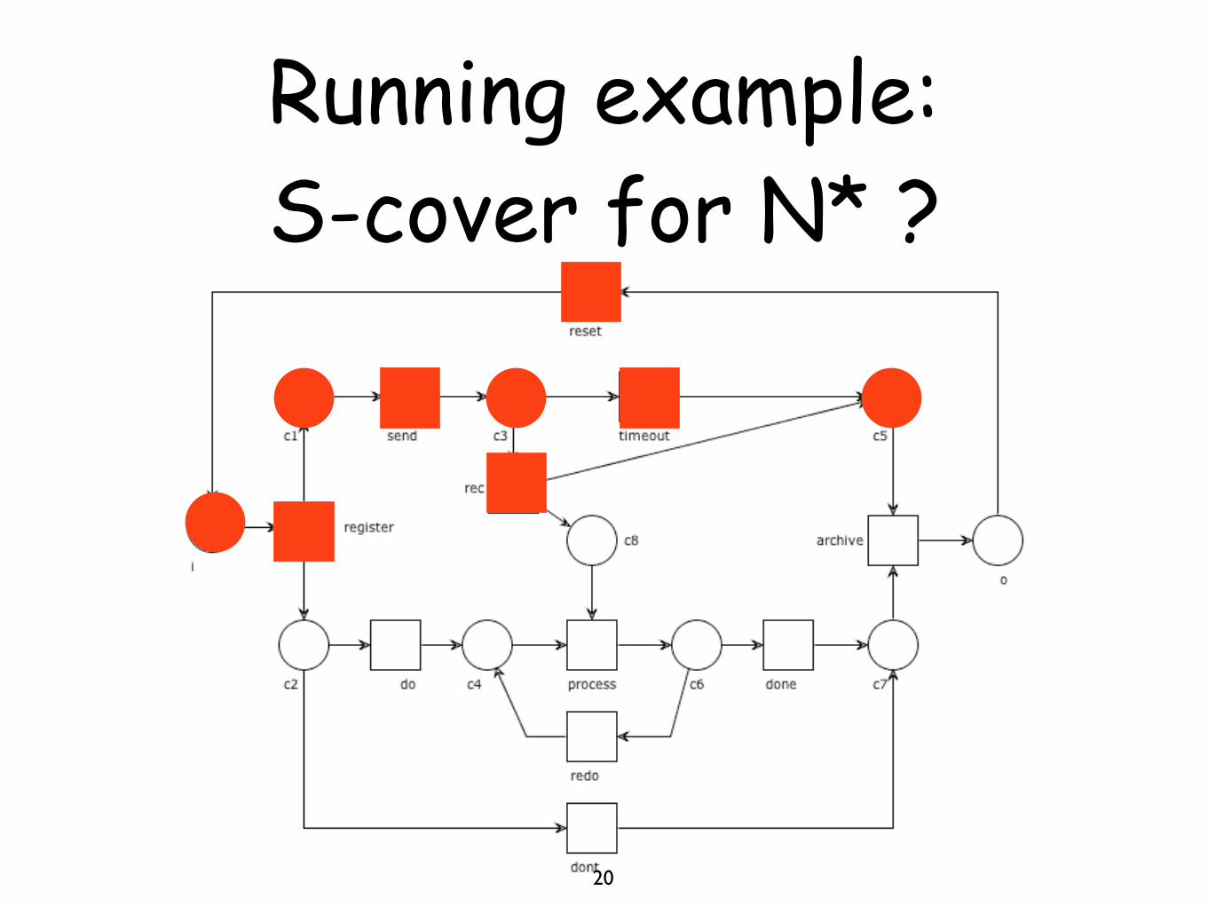
If N* is free-choice, live and bounded it must be S-coverable (S-coverability theorem)
(note that any S-component of N* includes i, o, reset, by strong-connectedness)
Corollary: If N is sound and free-choice, then N* must be S-coverable
N free-choice + N* not S-coverable => N not sound
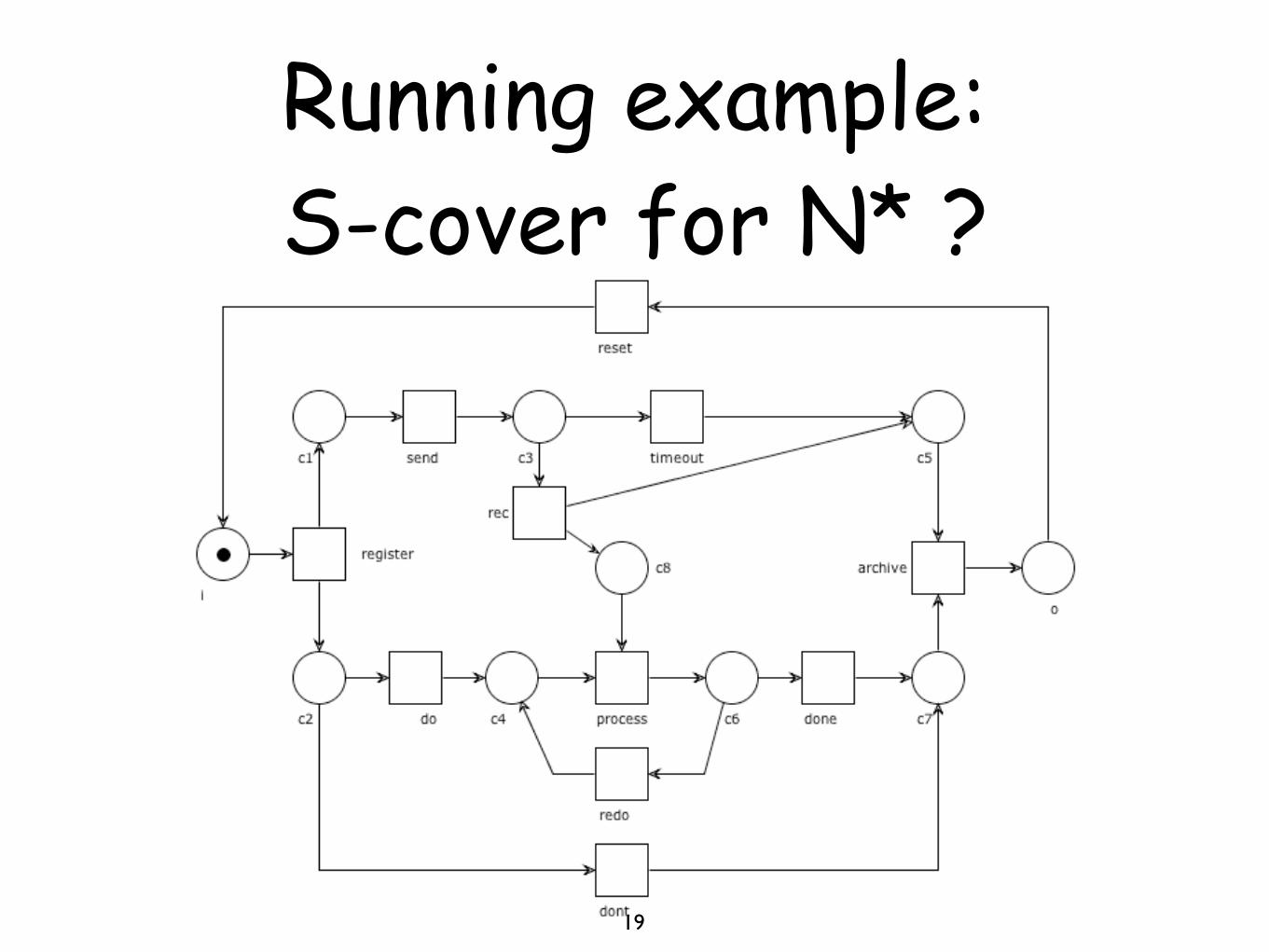
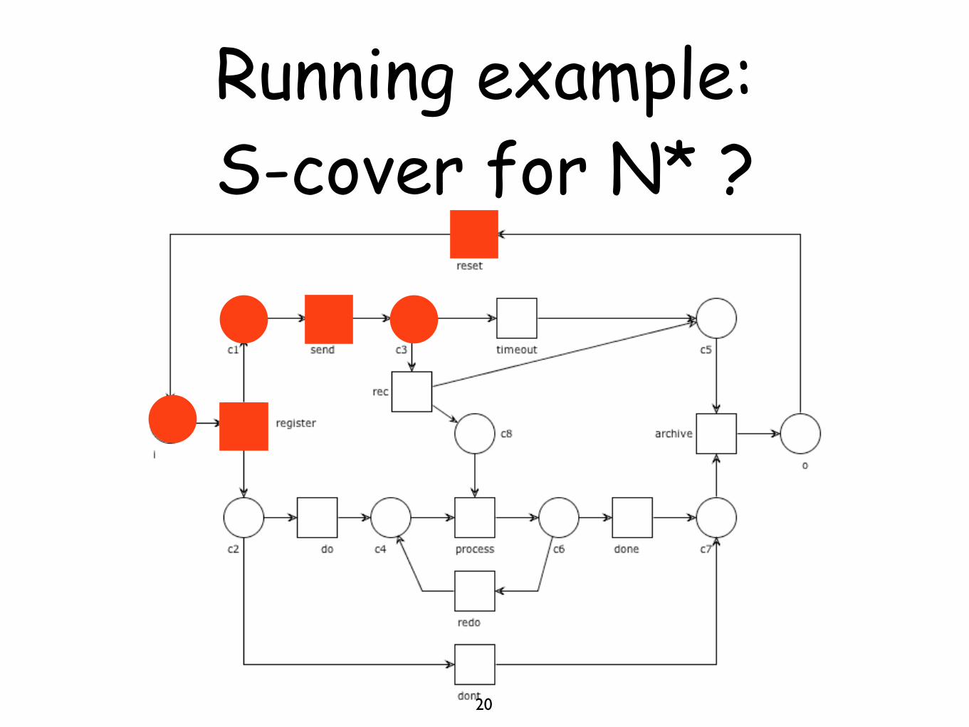
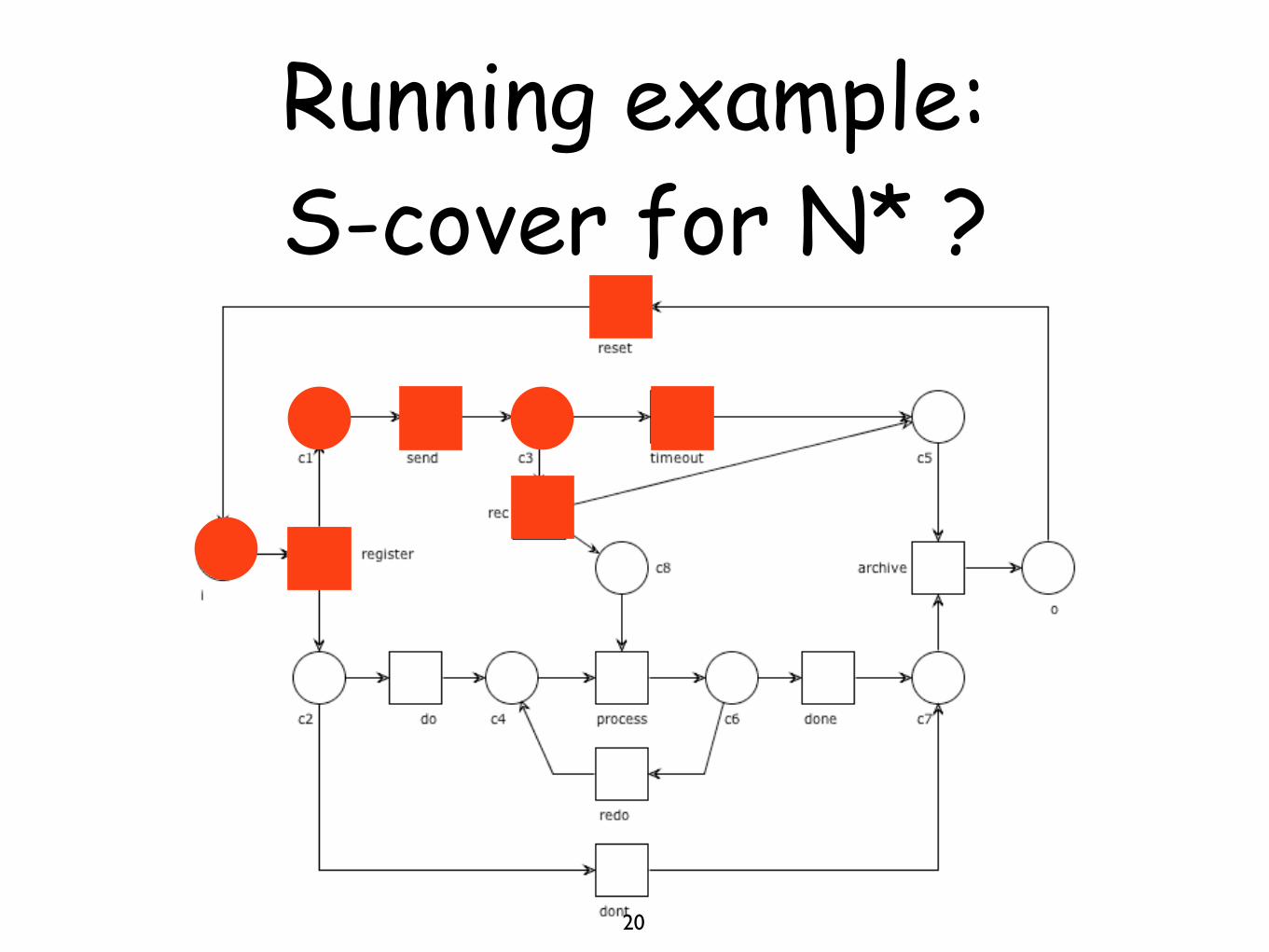
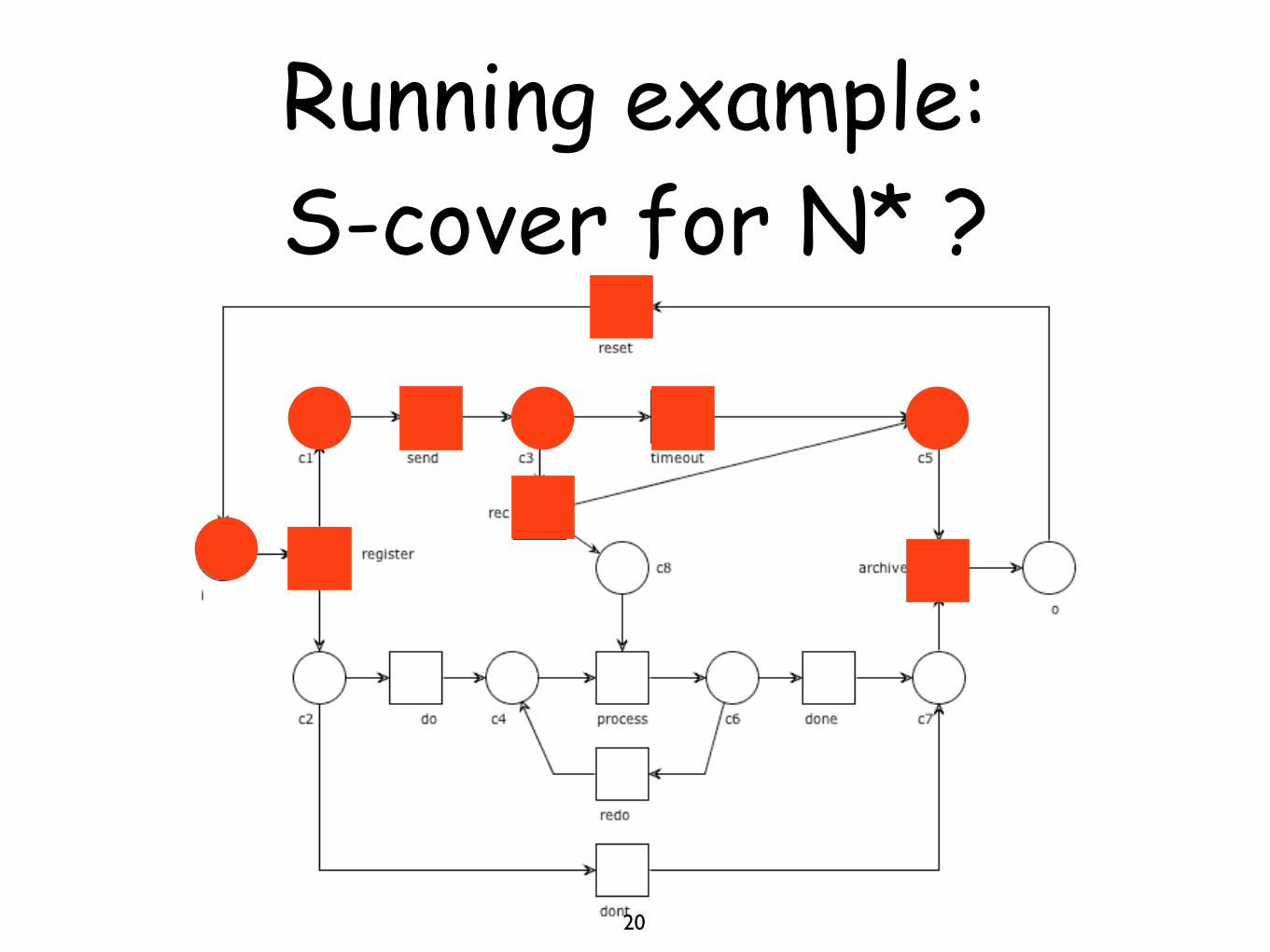
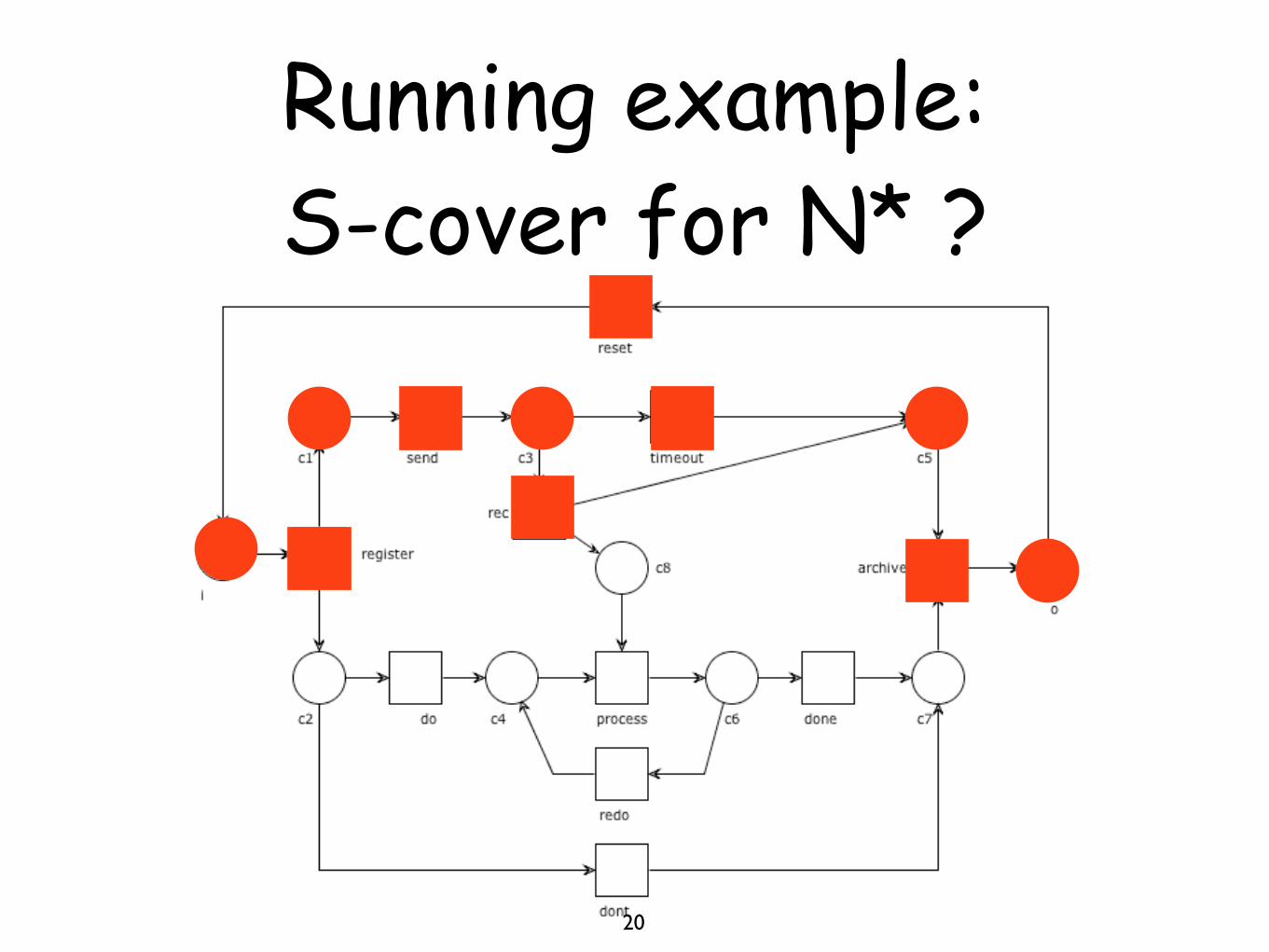
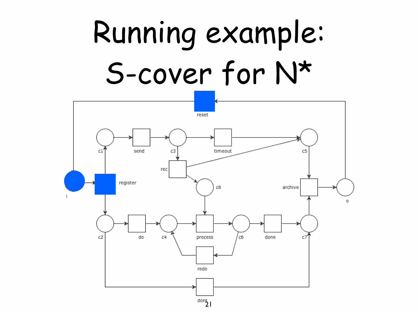
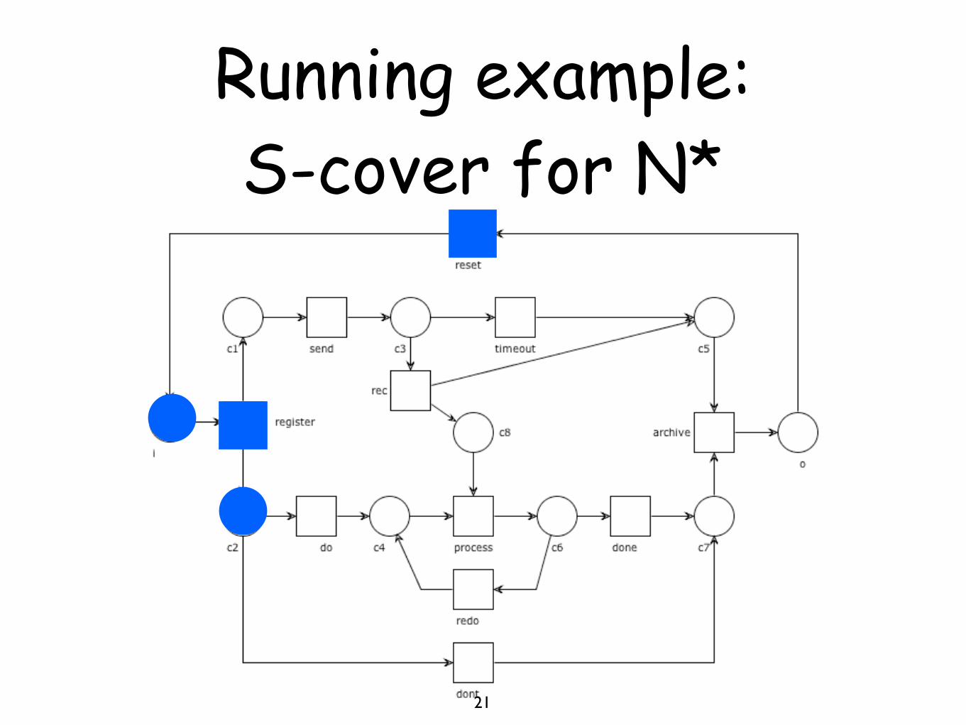
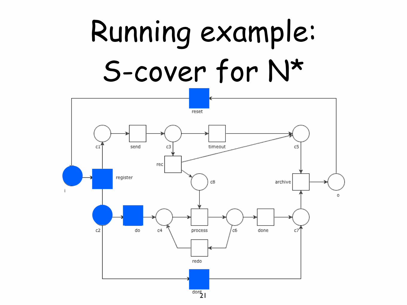
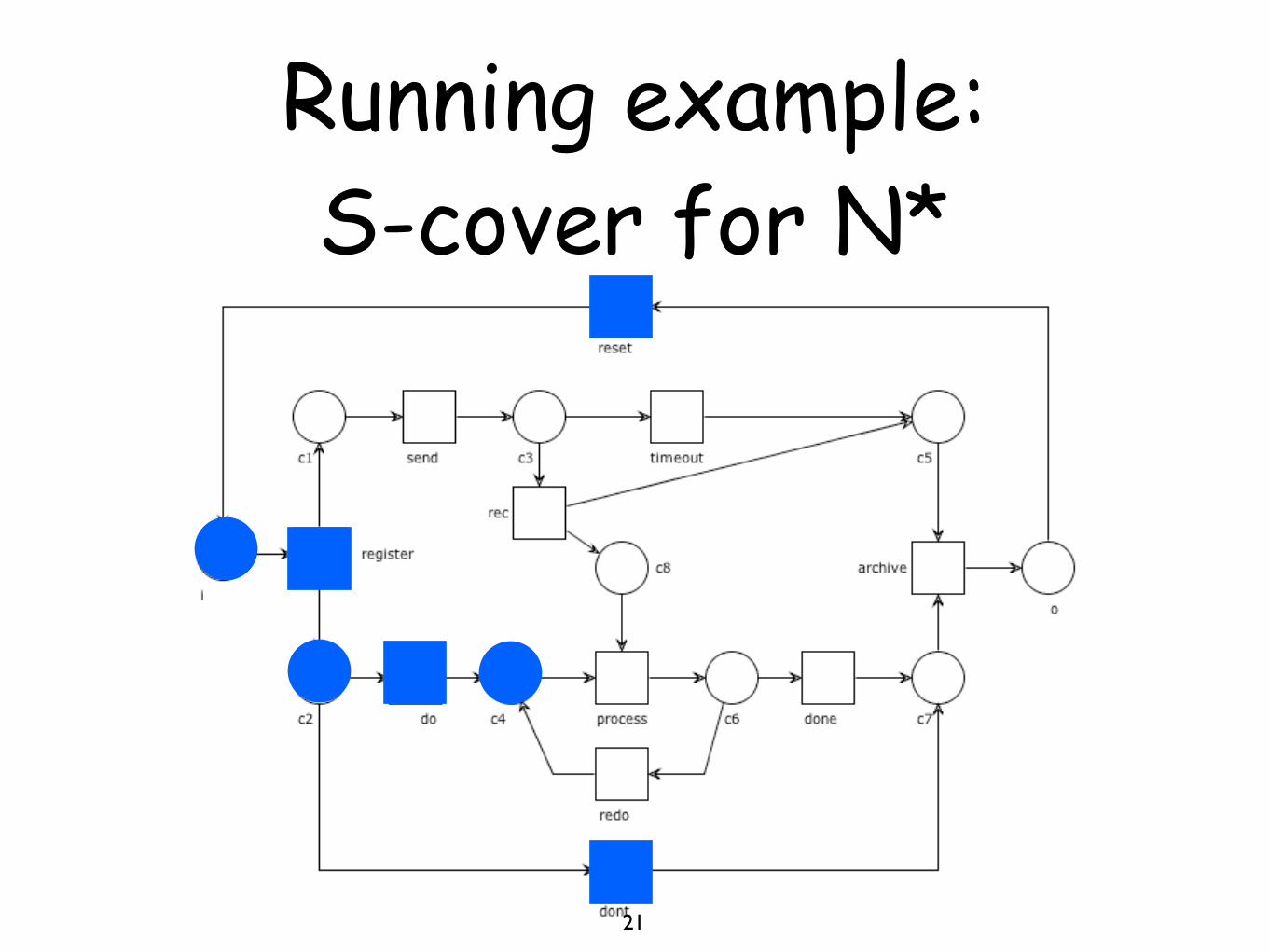
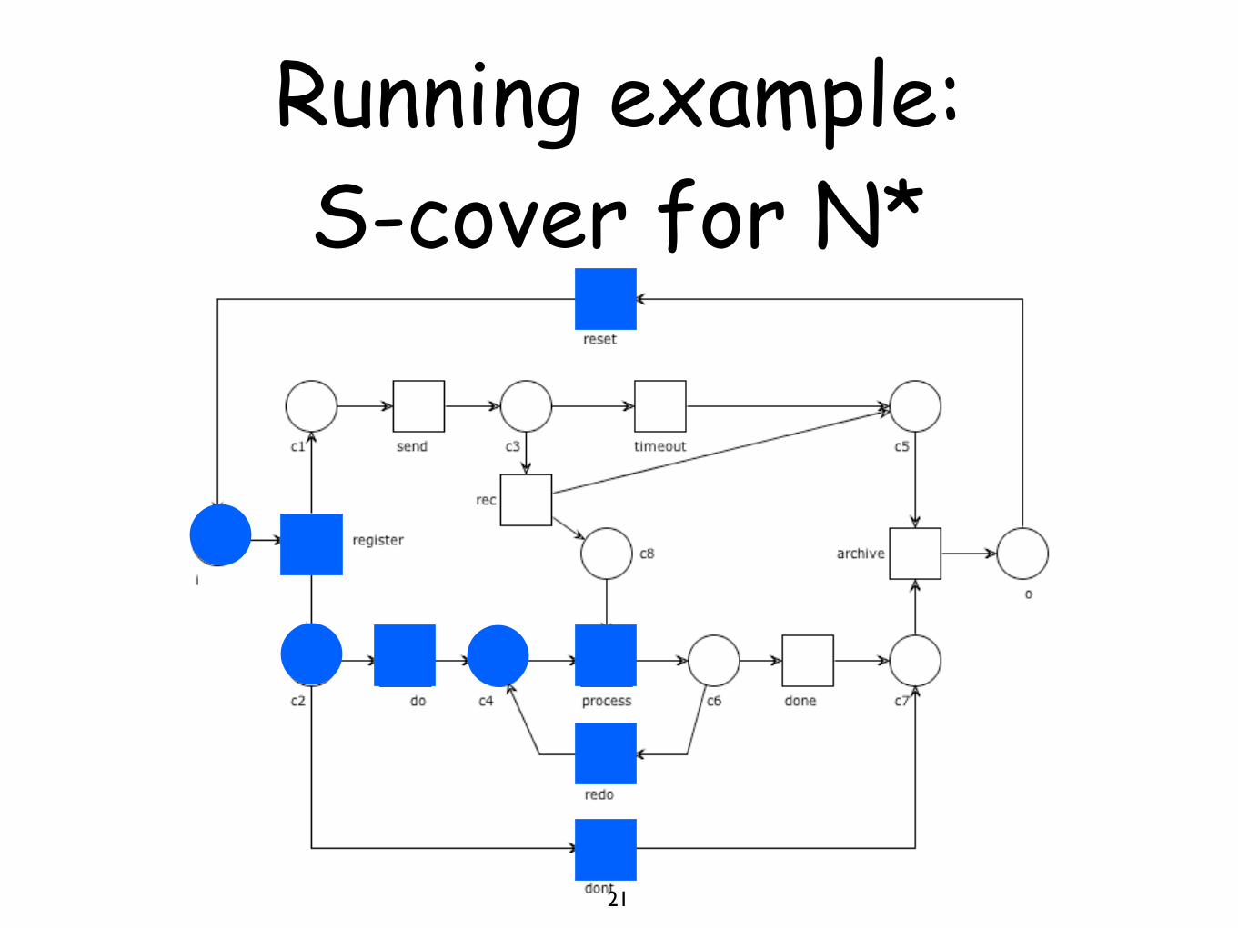
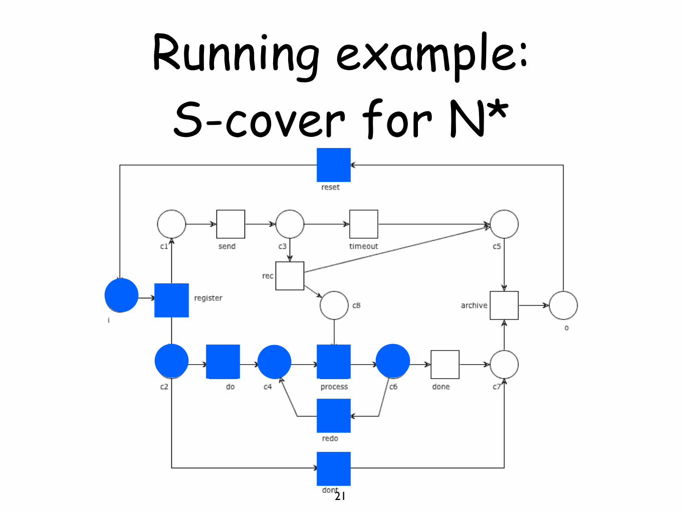
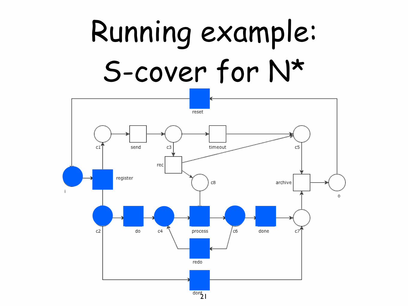
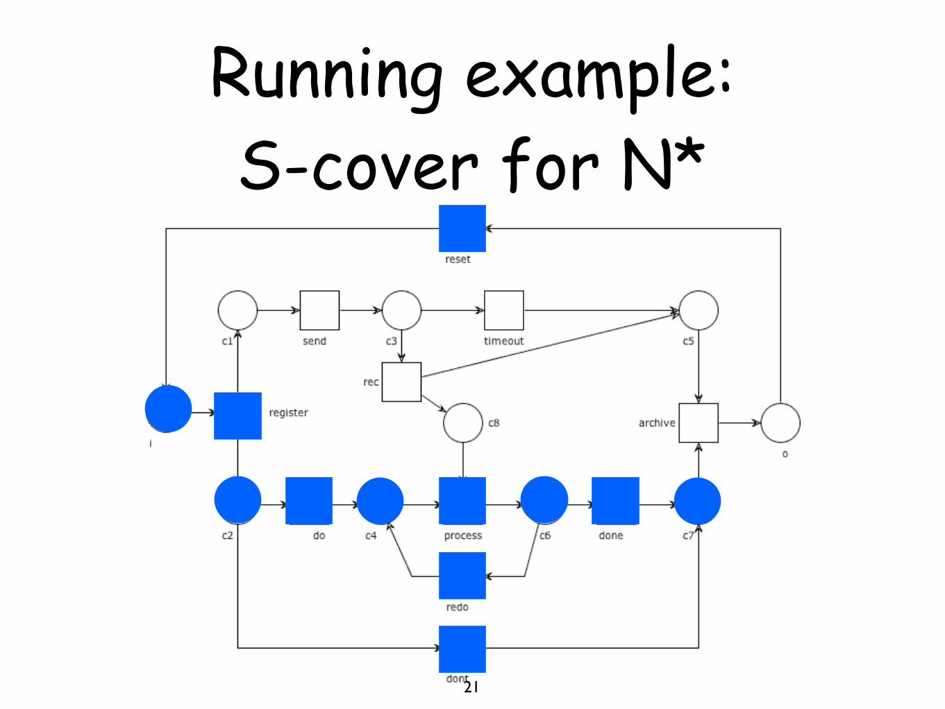
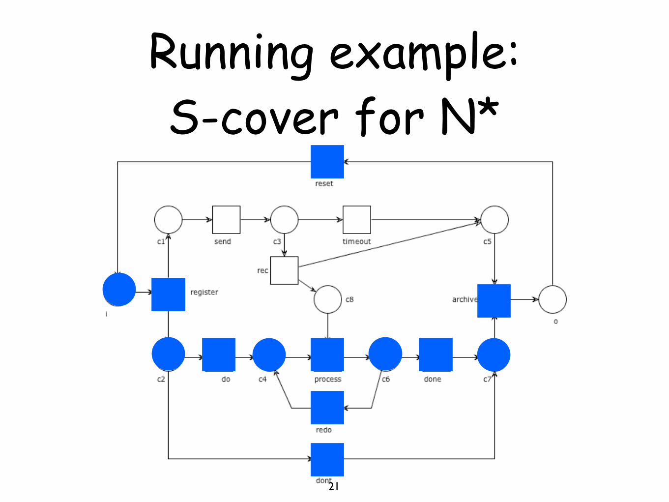
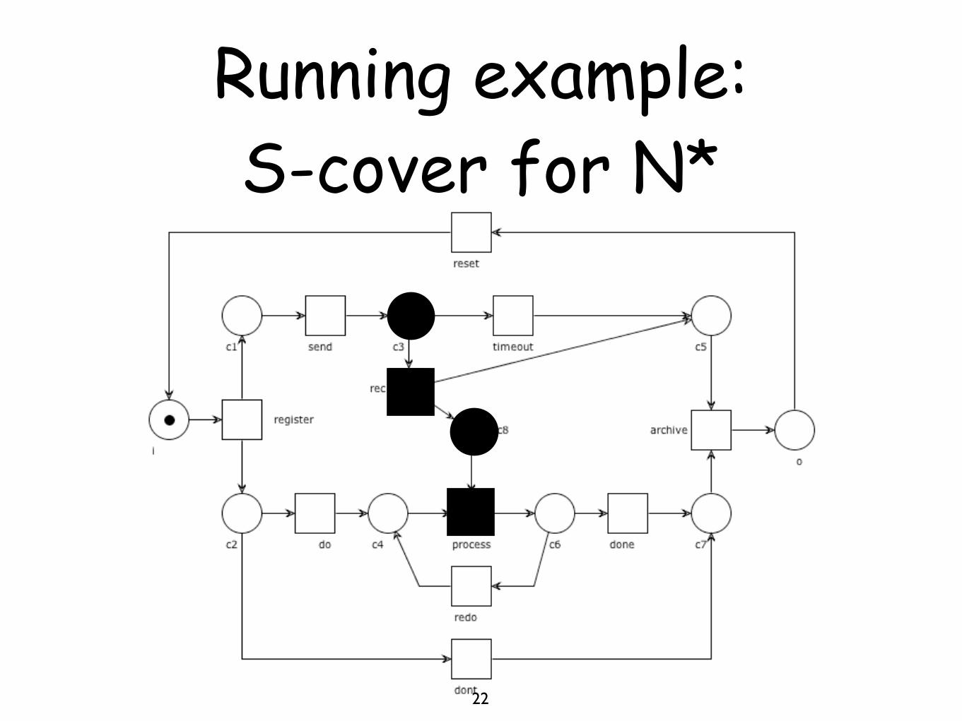
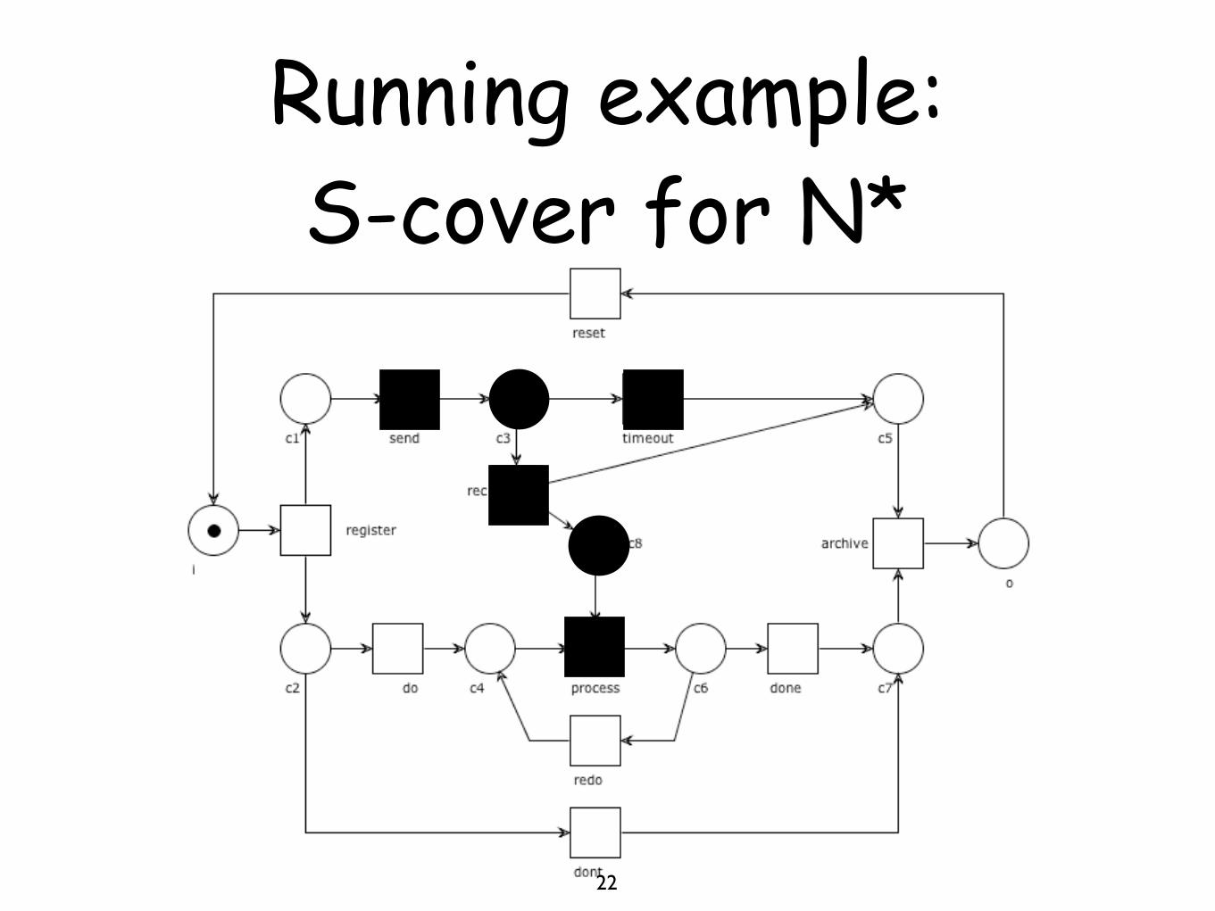
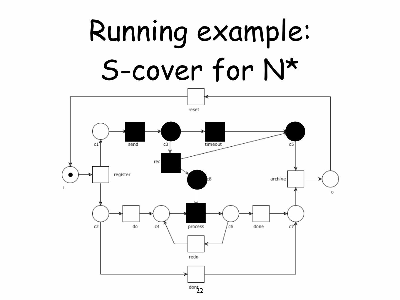
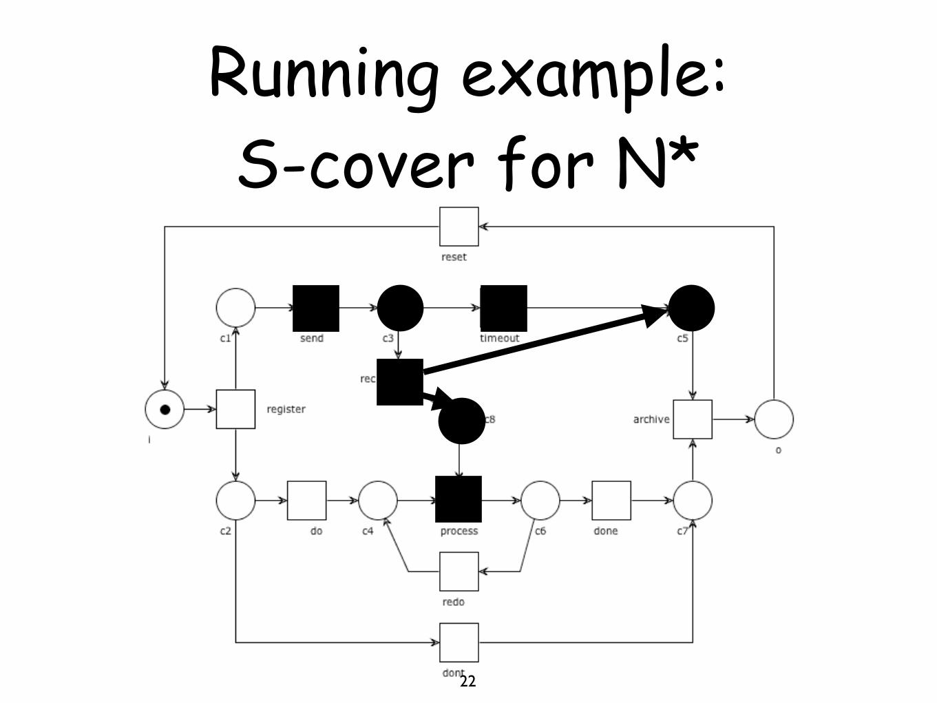
Running example: S-cover for N* ?
19
Running example: S-cover for N* ?
20
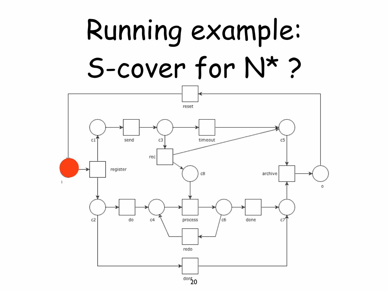
Running example: S-cover for N* ?
20
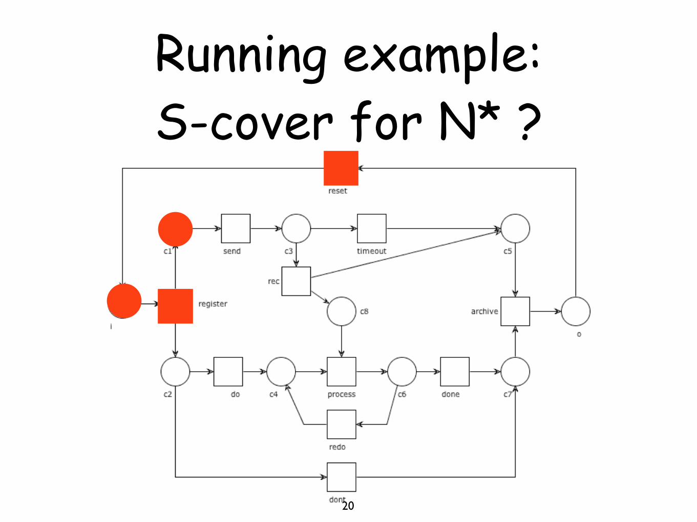
Running example: S-cover for N* ?
20
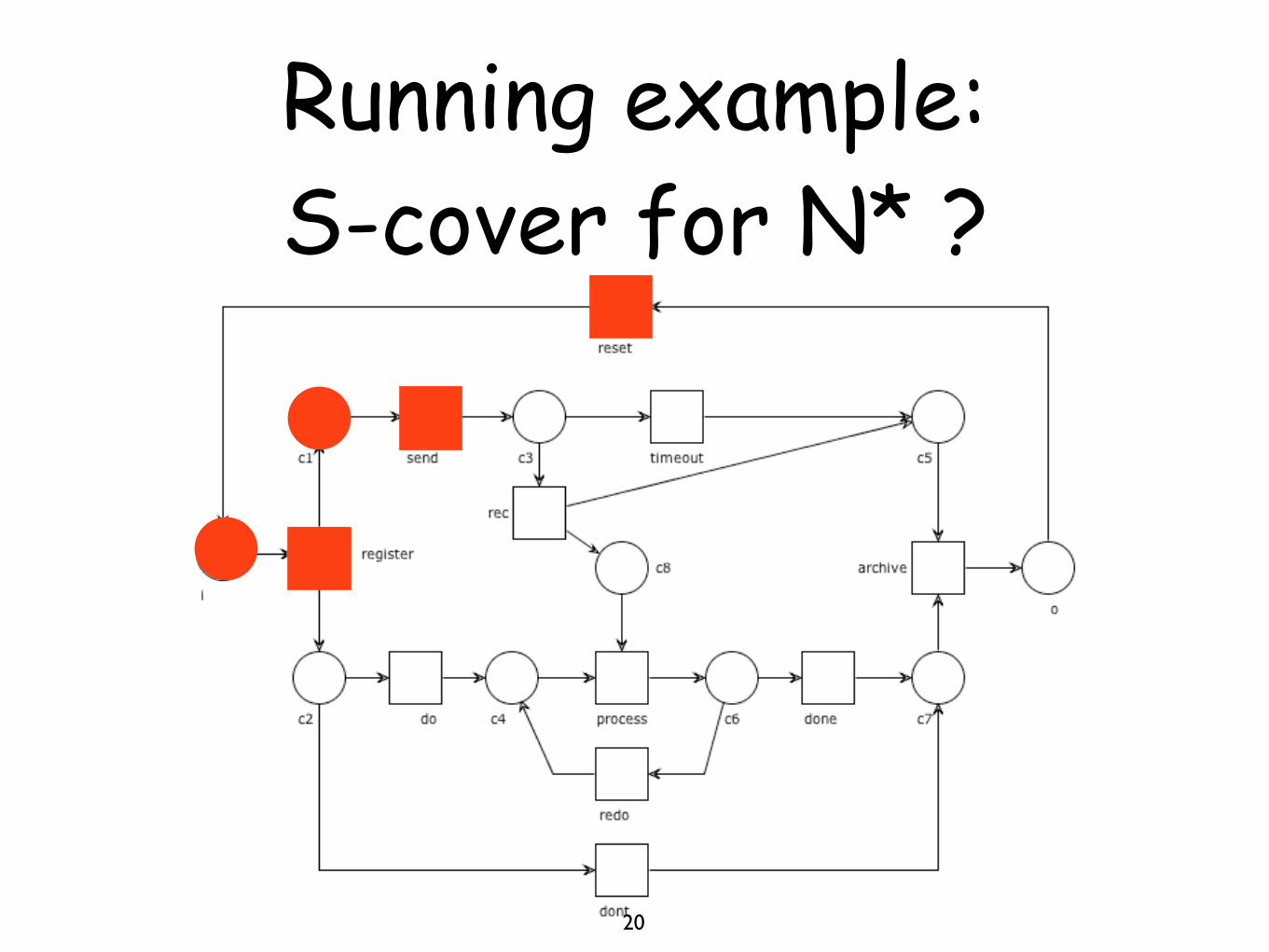
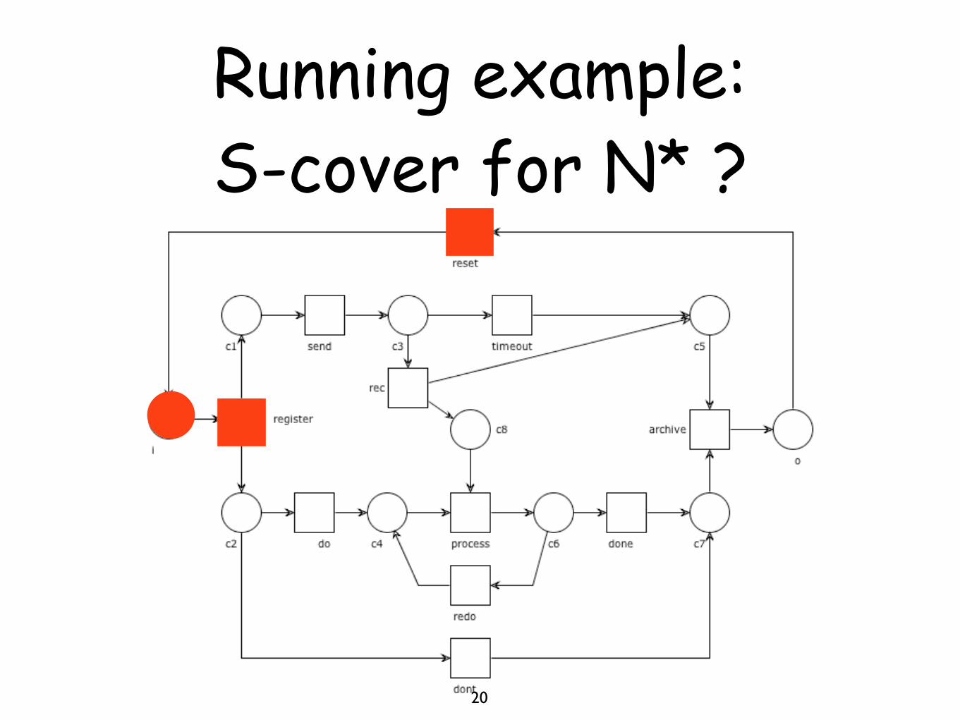
Running example: S-cover for N* ?
20
Running example: S-cover for N* ?
20
Running example: S-cover for N* ?
20
Running example: S-cover for N* ?
20
Running example: S-cover for N* ?
20
Running example: S-cover for N* ?
20
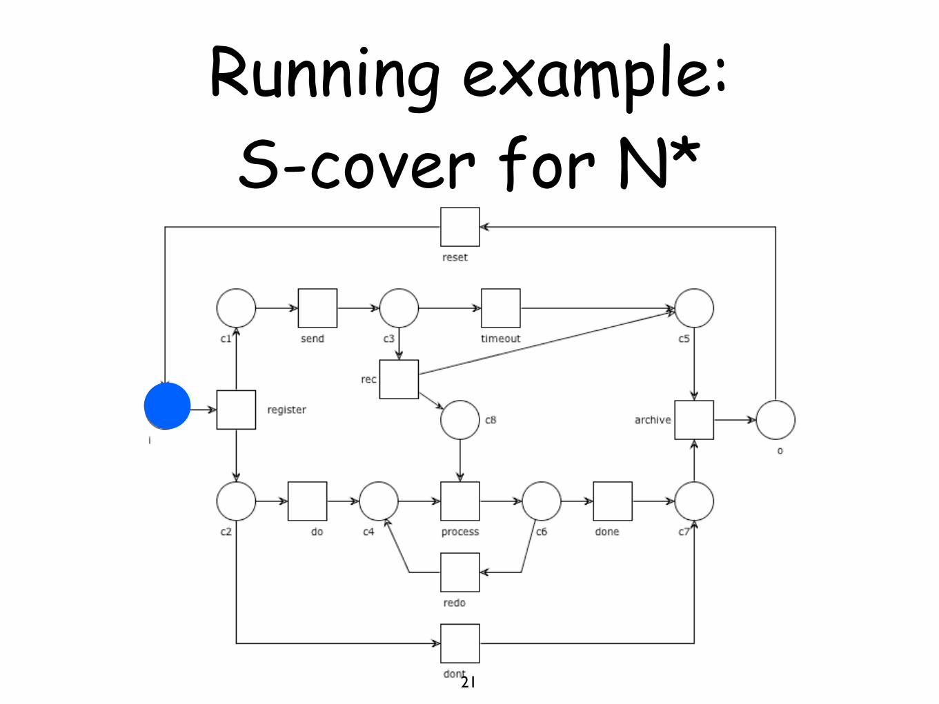
Running example: S-cover for N*
21
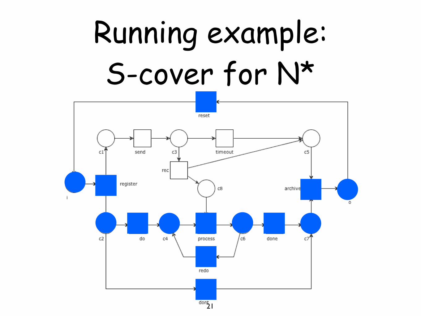
Running example: S-cover for N*
21
Running example: S-cover for N*
21
Running example: S-cover for N*
21
Running example: S-cover for N*
21
Running example: S-cover for N*
21
Running example: S-cover for N*
21
Running example: S-cover for N*
21
Running example: S-cover for N*
21
Running example: S-cover for N*
21
Running example: S-cover for N*
21
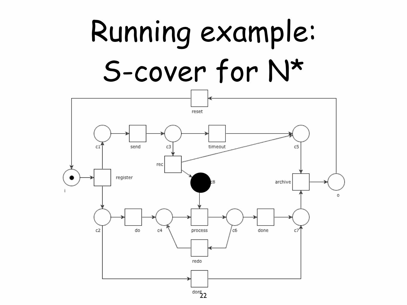
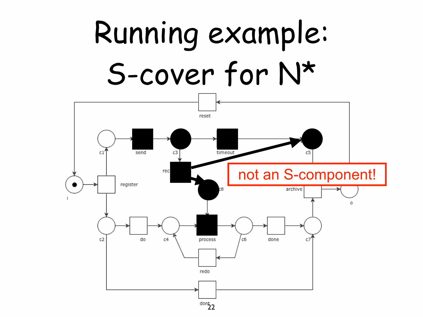
Running example: S-cover for N*
22
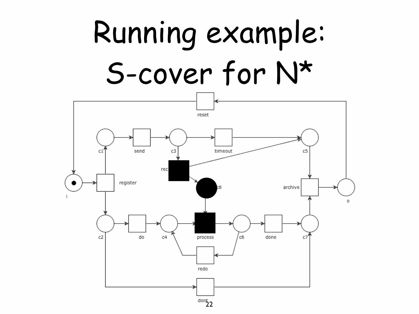
Running example: S-cover for N*
22
Running example: S-cover for N*
22
Running example: S-cover for N*
22
Running example: S-cover for N*
22
Running example: S-cover for N*
22
Running example: S-cover for N*
22
not an S-component!
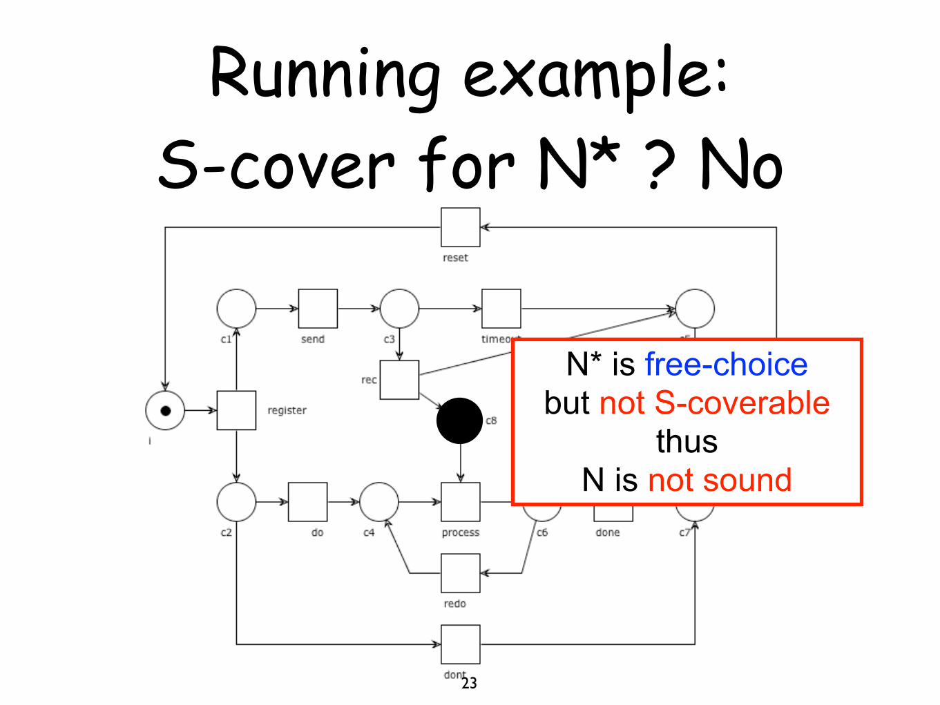
Running example: S-cover for N* ? No
23
N* is free-choice but not S-coverable
thus N is not sound
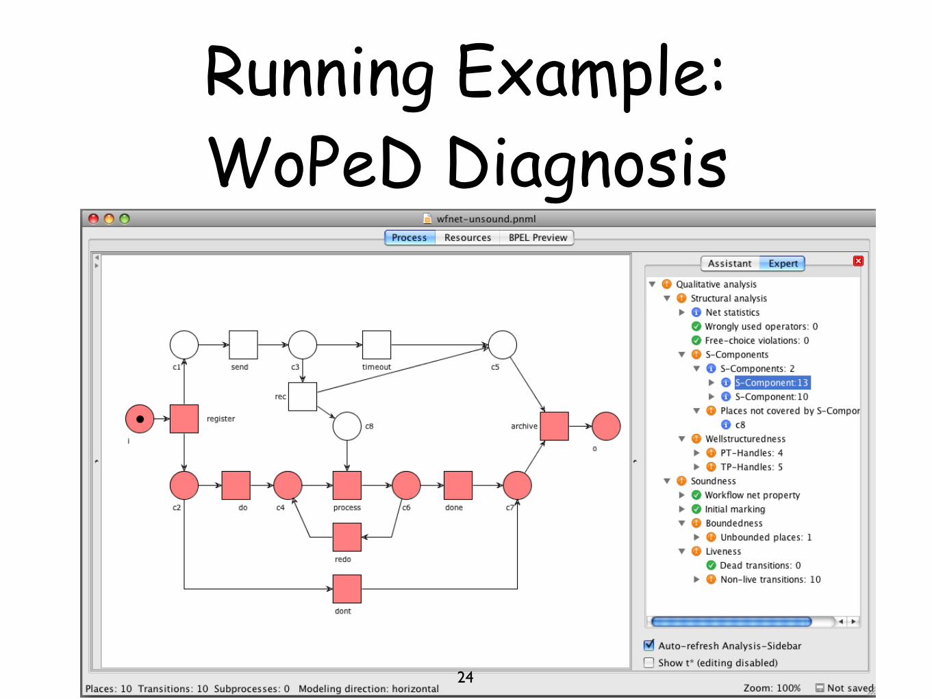
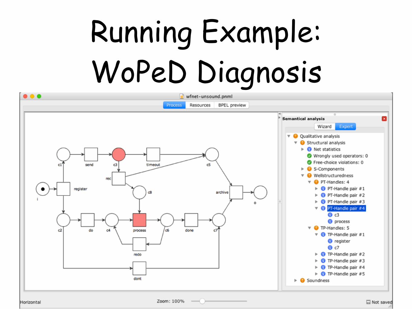
Running Example: WoPeD Diagnosis
24
Split / Join Balancing
25
A good workflow design is characterized by a balance between AND/XOR-split and AND/XOR-joins
Any mismatch is a potential source of errors
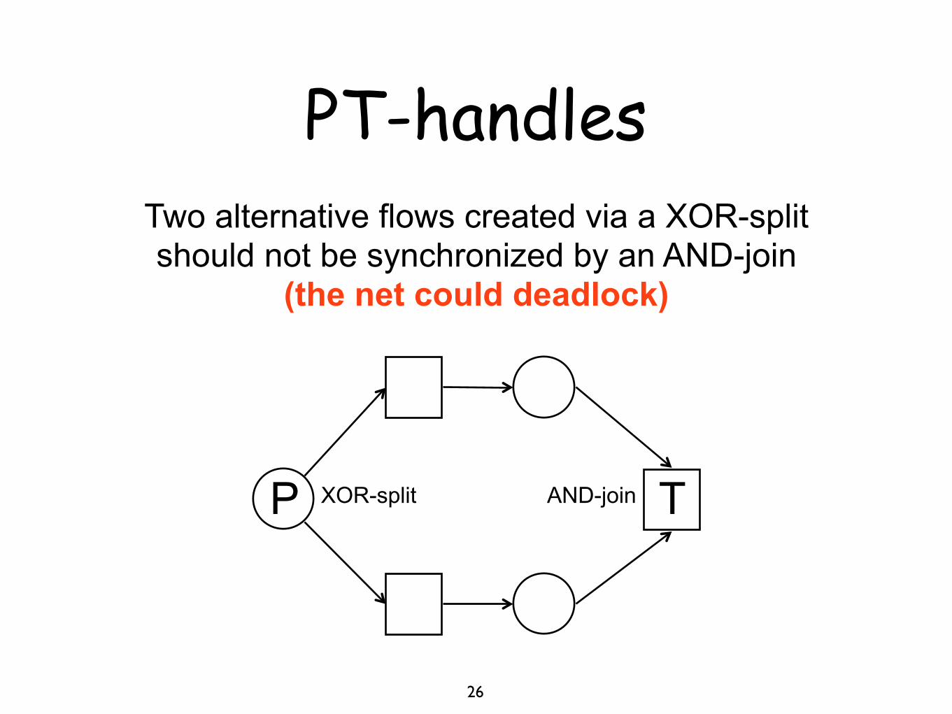
26
Two alternative flows created via a XOR-split should not be synchronized by an AND-join
(the net could deadlock)
PT-handles
TP XOR-split AND-join
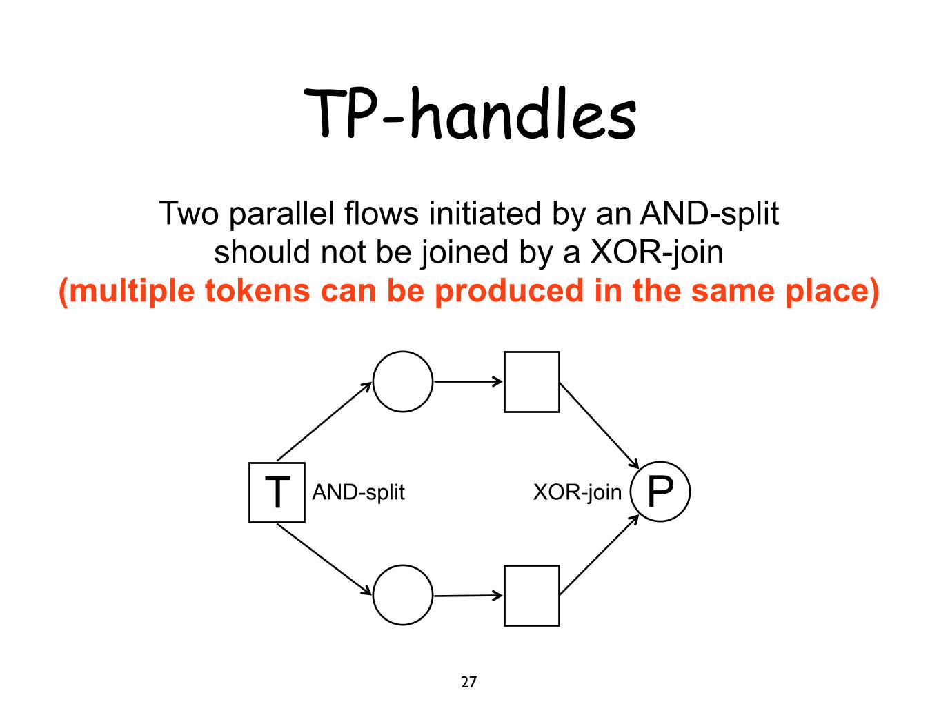
27
Two parallel flows initiated by an AND-split should not be joined by a XOR-join
(multiple tokens can be produced in the same place)
TP-handles
T PAND-split XOR-join
TP- and PT-handles
28
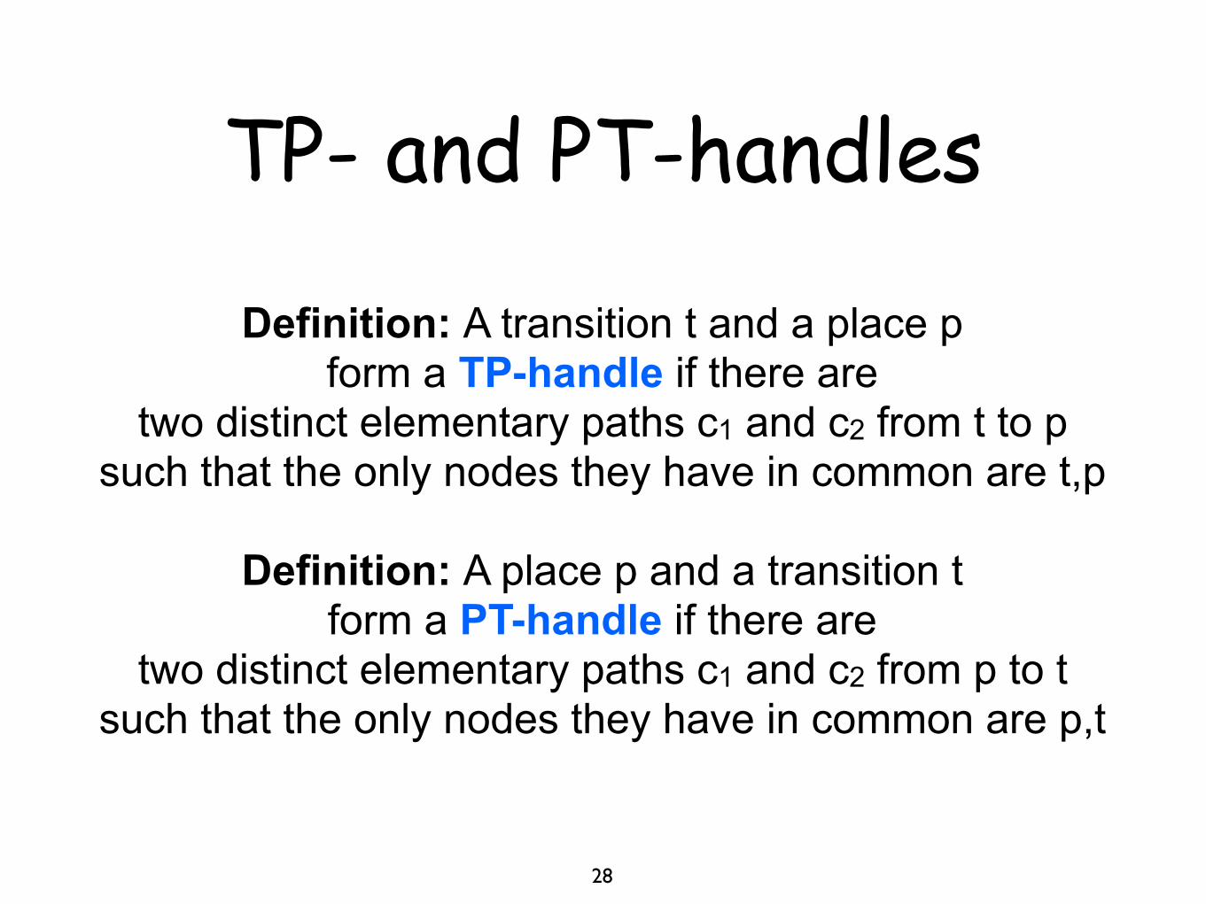
Definition: A transition t and a place p form a TP-handle if there are
two distinct elementary paths c1 and c2 from t to p such that the only nodes they have in common are t,p
Definition: A place p and a transition t form a PT-handle if there are
two distinct elementary paths c1 and c2 from p to t such that the only nodes they have in common are p,t
Well-Structured Nets
29
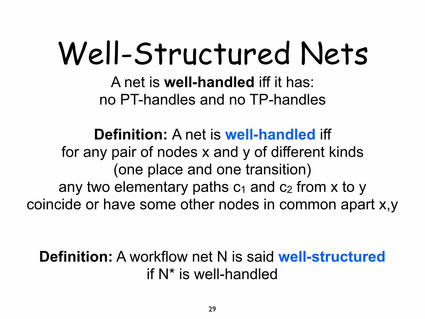
A net is well-handled iff it has: no PT-handles and no TP-handles
Definition: A net is well-handled iff for any pair of nodes x and y of different kinds
(one place and one transition) any two elementary paths c1 and c2 from x to y
coincide or have some other nodes in common apart x,y
Definition: A workflow net N is said well-structured if N* is well-handled
S-coverability diagnosis
30
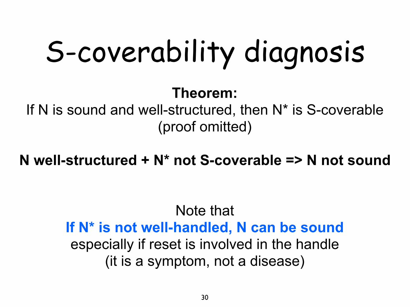
Theorem: If N is sound and well-structured, then N* is S-coverable
(proof omitted)
N well-structured + N* not S-coverable => N not sound
Note that If N* is not well-handled, N can be sound especially if reset is involved in the handle
(it is a symptom, not a disease)
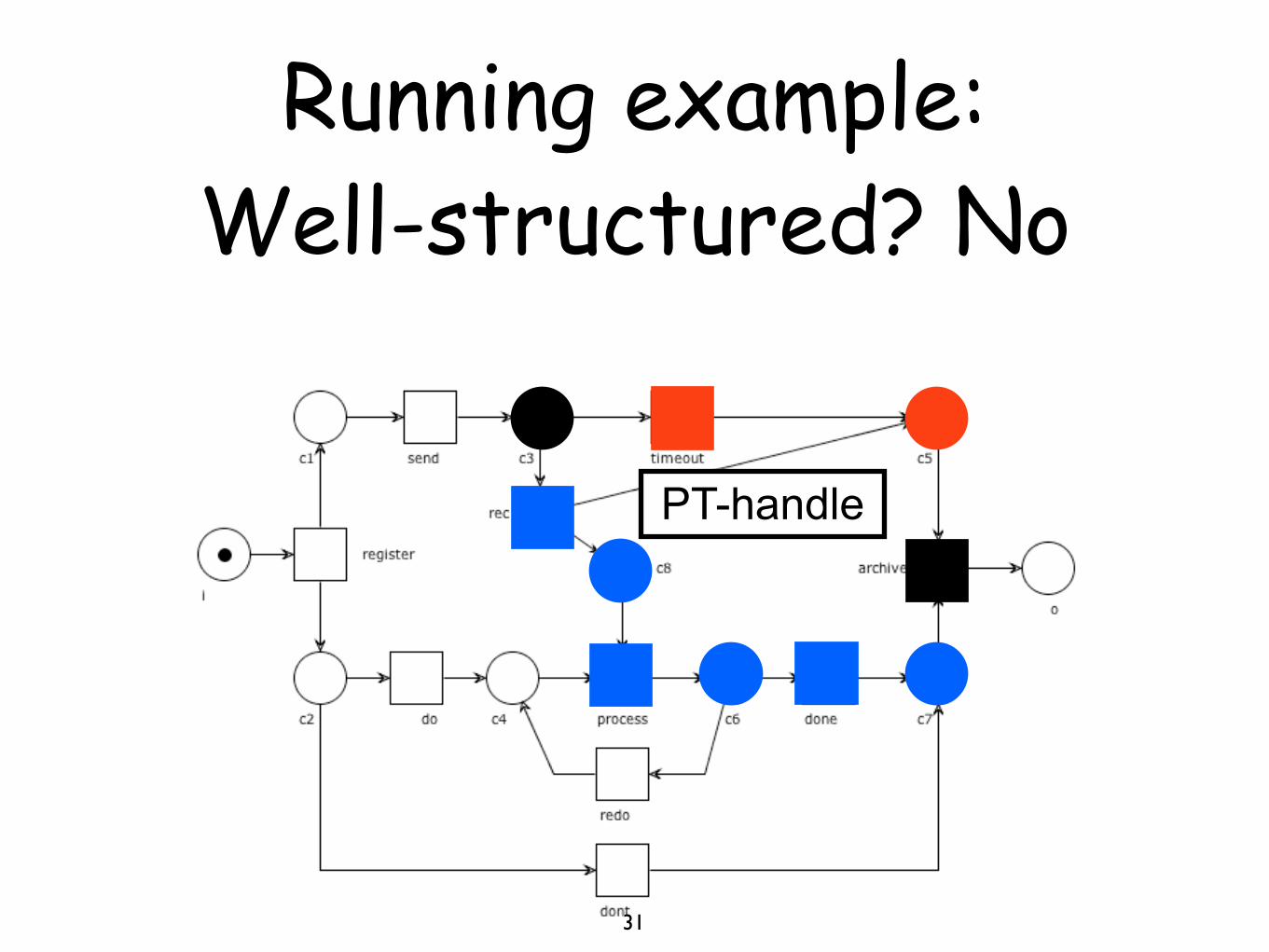
Running example: Well-structured? No
31
PT-handle
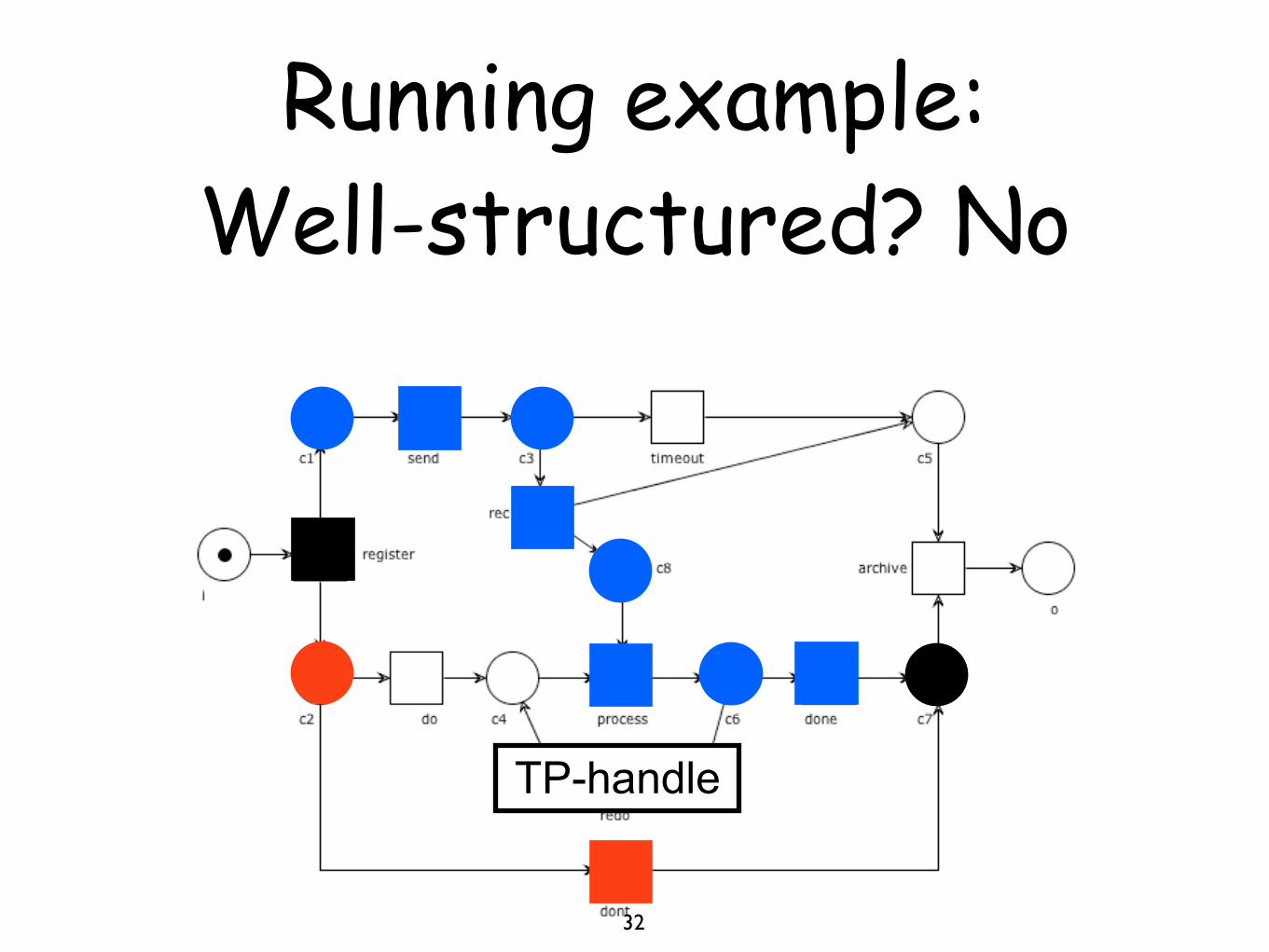
Running example: Well-structured? No
32
TP-handle
Be careful
33
N well-structured = N* well-handled
WoPeD marks PT/TP-handles over N* (not over N)
Running Example: WoPeD Diagnosis
34
Liveness and boundedness vs
Soundness requirements
35
Improper completion
36
Suppose N completes improperly: from i we can reach o+M
We can do the same on N* then we fire reset and reach i+M
we can repeat the same run and reach i+2M and then i+3M and then i+4M and then ... i+kM
then N* has some unbounded places (all p such that M(p)>0)

Unsoundness from unboundedness
37
Improper completion of N implies unboundeness of N*
Symptom: N* has some unbounded places
Disease: N could complete improperly
Consequences of boundedness
38
If N* is bounded, then: if o+M is reachable from i in N, then M=0
If N* is bounded, then either N satisfies
both option to complete and proper completion or N does not satisfy option to complete
Completion option failure
39
Suppose N does not satisfy the “option to complete”: then from i we can reach M
from which we cannot mark o
We can do the same on N* then reset is dead from M i.e. reset is non-live in N*
N* has non-live transitions (including reset)
Unsoundness from non-liveness
40
Option to complete fail for N implies non-liveness of N*
Symptom: reset transition is non-live in N*
Disease: N could violate option to complete
Unsoundness from Non-Liveness
41
If N* is bounded and has dead transitions, then
if reset is dead N and N* have the same finite reachability graph
hence N has the same dead tasks as N* (except reset)
if reset is not dead the reachability graphs of N and N* differ only for
(because N* is bounded) hence N has the same dead tasks as N*
oreset�⇥ i
Unsoundness from Non-Liveness
42
Symptom: N* is bounded and has dead transitions
Disease: N has the same dead tasks as N*
Unsoundness from Non-Liveness
43
Symptom: N* has non-live transitions
Disease: N could have dead transitions
(but which ones?)
Error sequences
44
Diagnostic information
45
The sets of: unbounded places of N* dead transitions of N*
non-live transitions of N*
may provide useful information for the diagnosis of behavioural errors (pointing to different types of errors)
Unfortunately, this information is not always sufficient to determine the exact cause of the error
Behavioural error sequences can overcome this problem
Error sequences
46
Rationale: We want to find firing sequences such that:
every continuation of such sequences will lead to an error
they have minimal length (none of its prefixes satisfies the above property)
Informally: error sequences are scenarios that capture
the essence of errors made in the workflow design (violate “option to complete” or “proper completion”)
Non-Live sequences: informally
47
A non-live sequence is a firing sequence of minimal length
such that completion of the case is no longer possible
i.e. a witness for transition reset being non-live in N*

Non-Live sequences: fundamental property
48
Let N be such that: N* is bounded
N (or equivalently N*) has no dead task
Then, N* is live iff
N has no non-live sequences
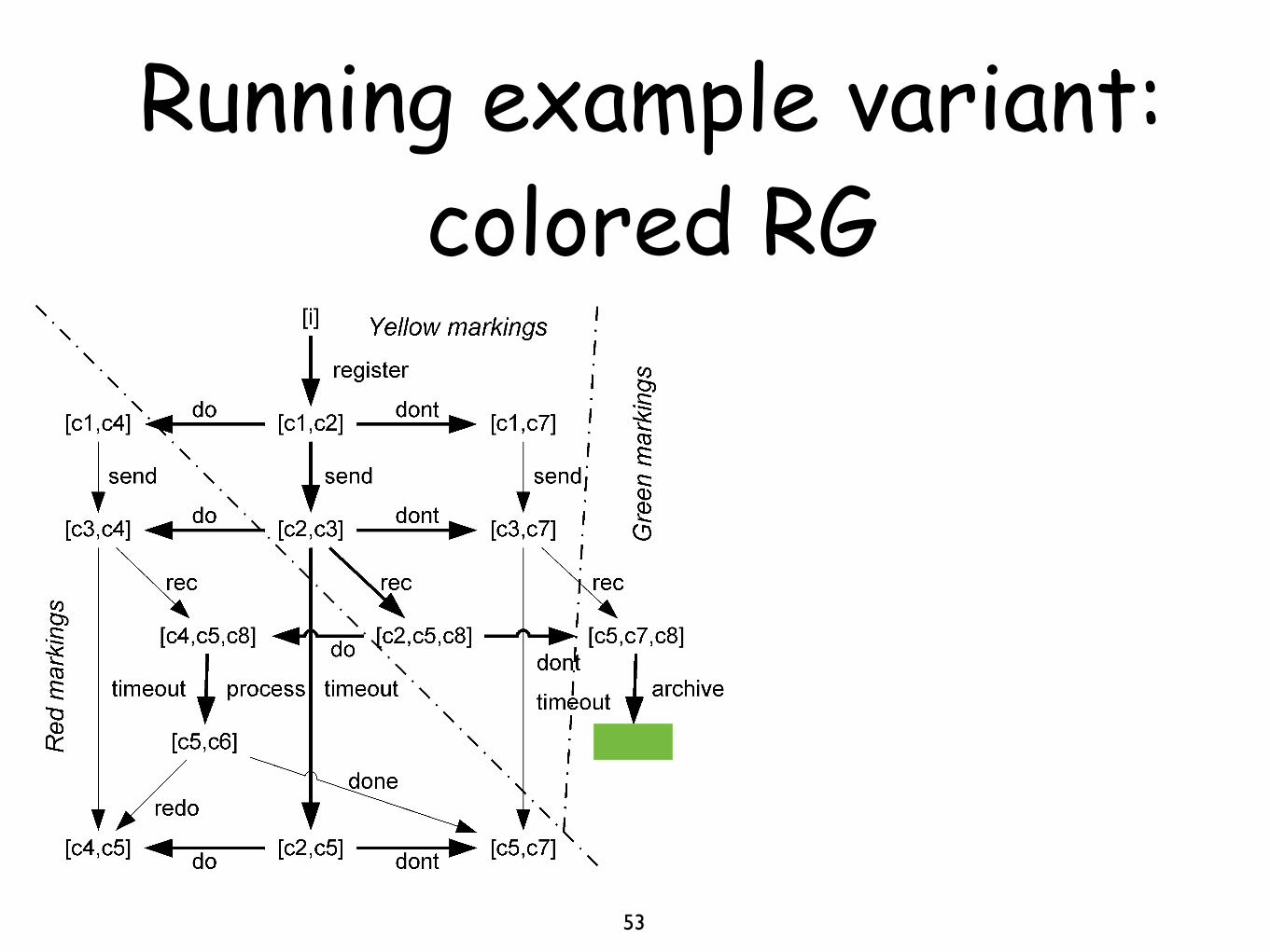
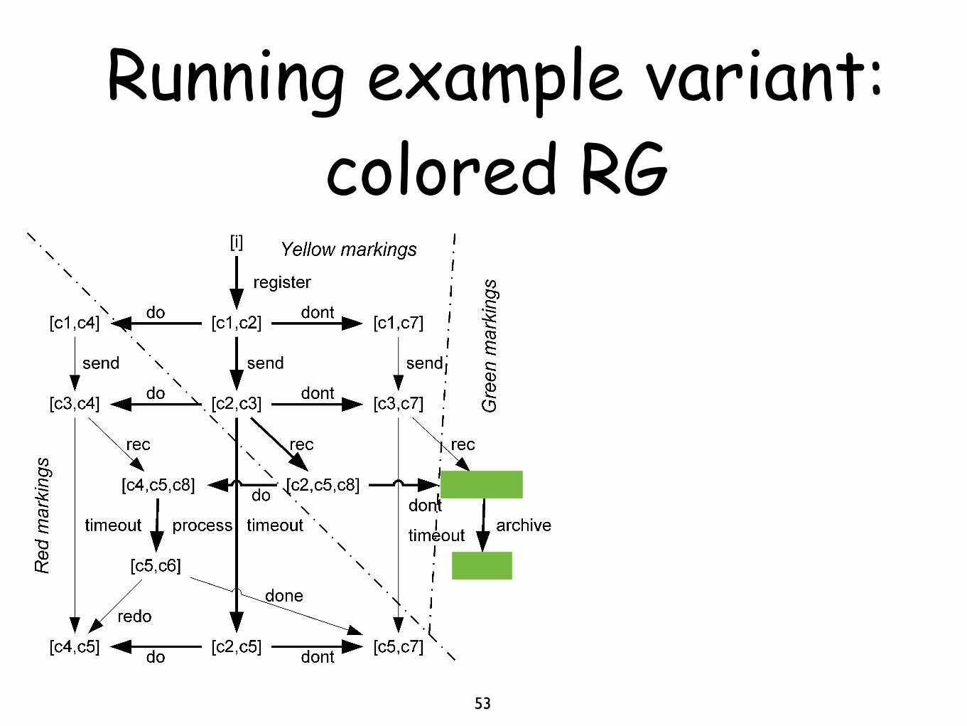
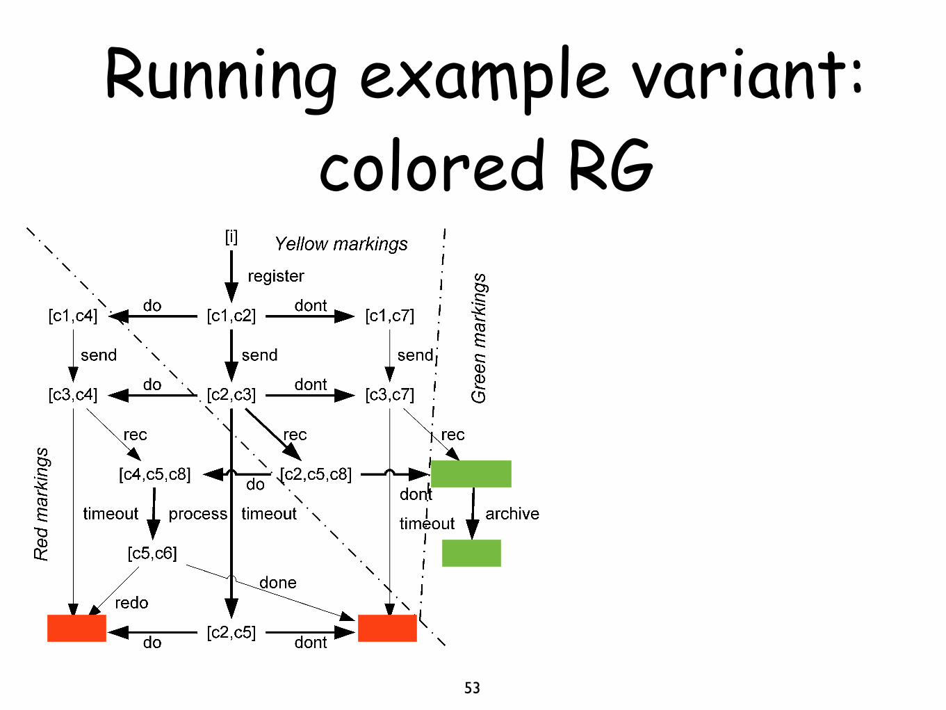
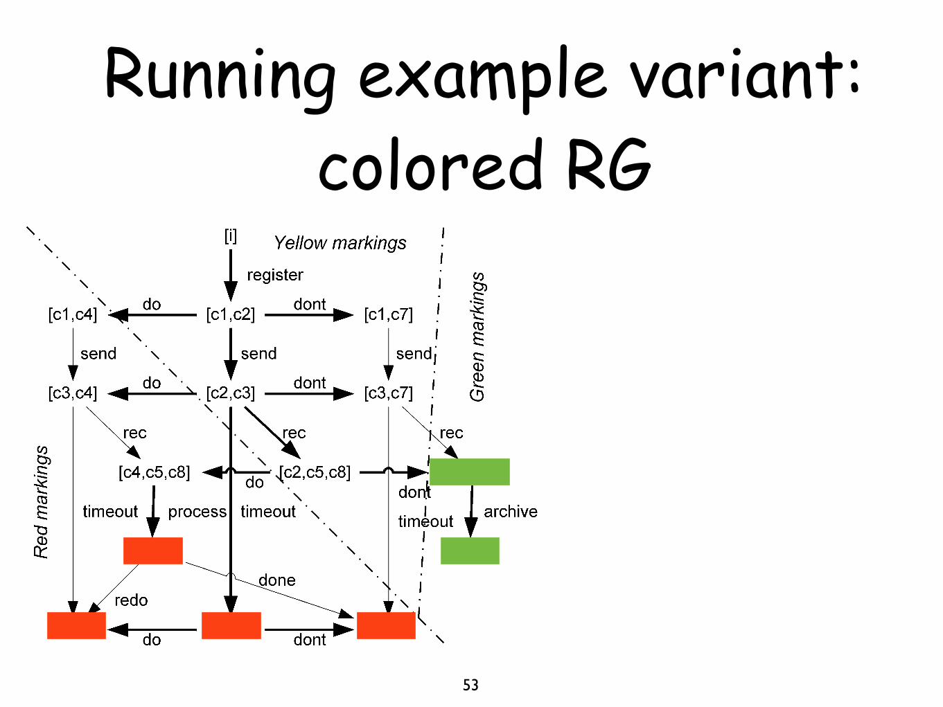
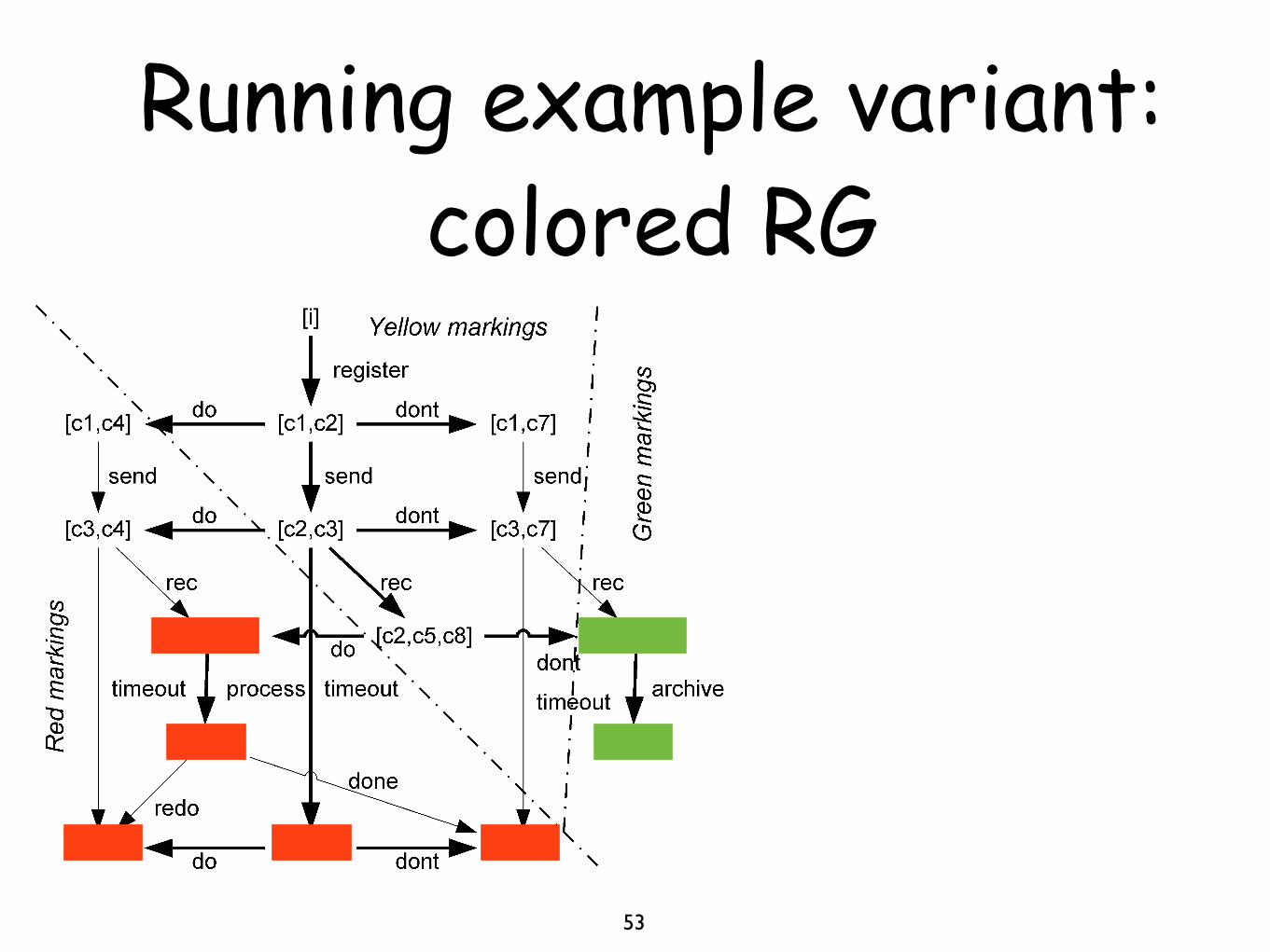
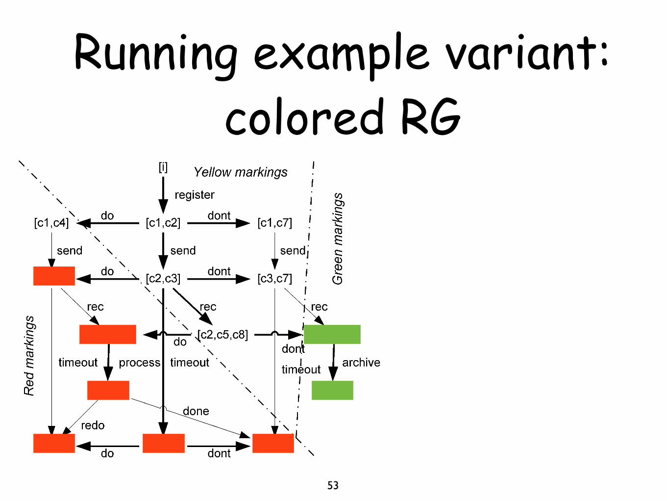
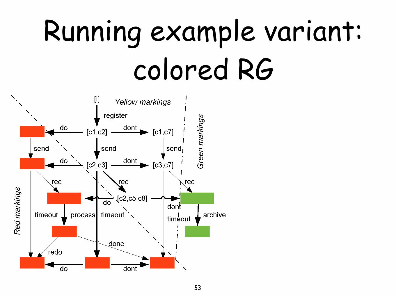
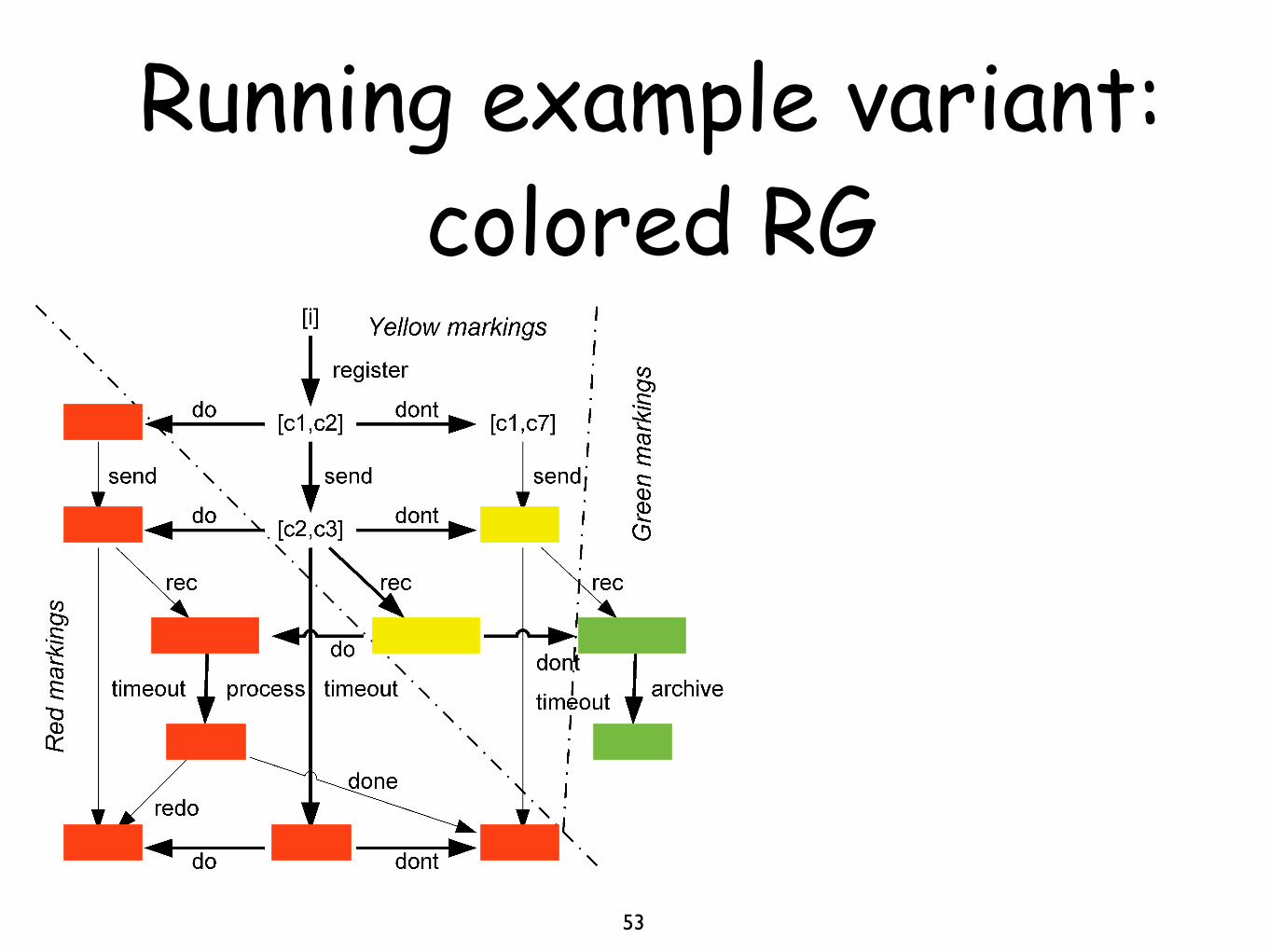
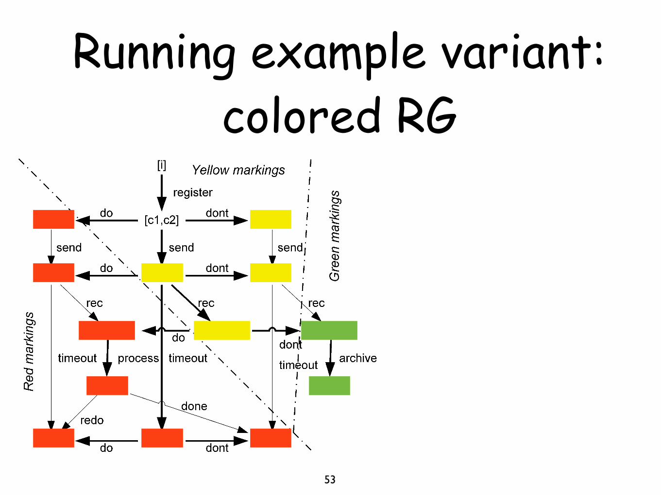
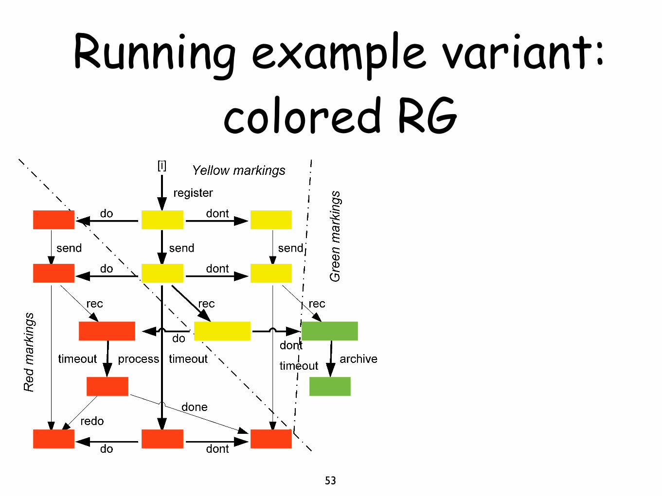
Non-Live sequences: graphically
49
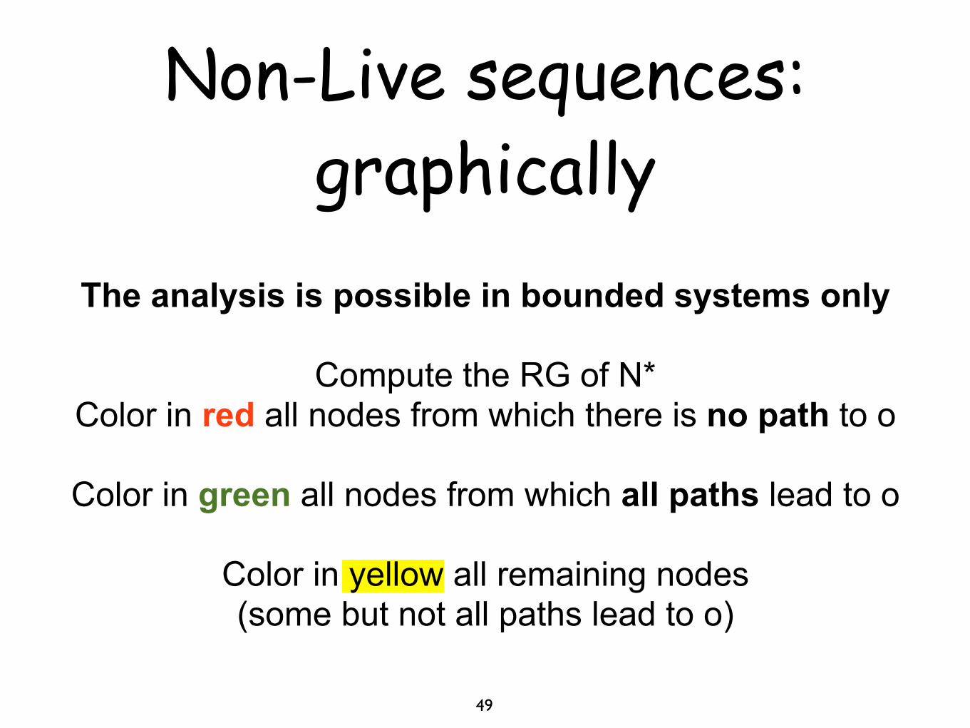
The analysis is possible in bounded systems only
Compute the RG of N* Color in red all nodes from which there is no path to o
Color in green all nodes from which all paths lead to o
Color in yellow all remaining nodes (some but not all paths lead to o)
Non-Live sequences: remarks
50
No red node implies no yellow node
No green node implies no yellow node
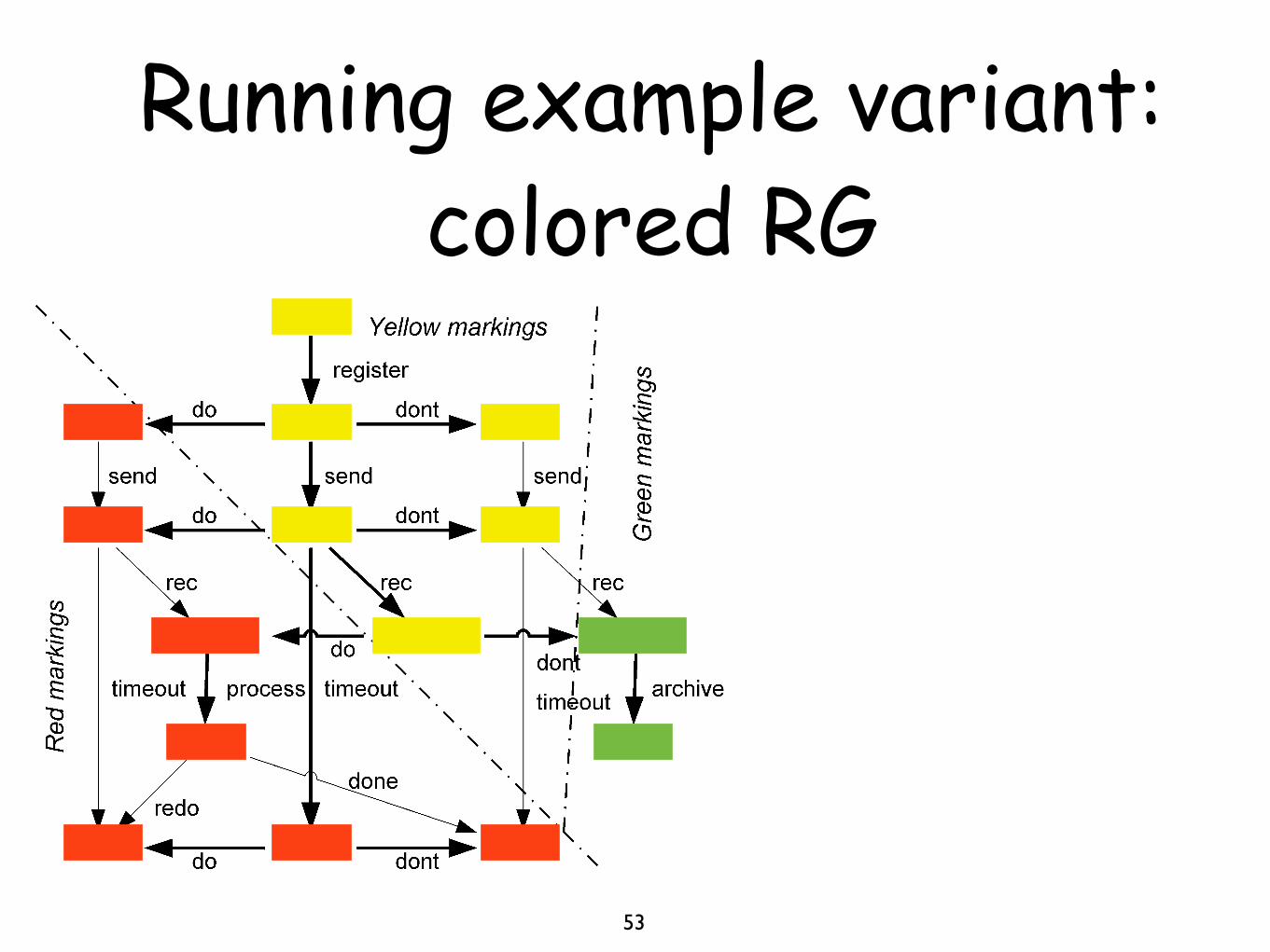
Non-Live sequences: formally
51
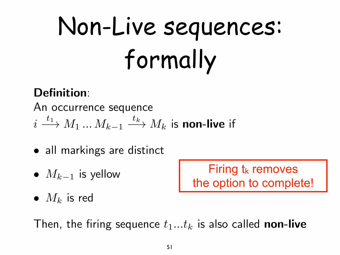
Definition:An occurrence sequence
it1�⇥ M1 ...Mk�1
tk�⇥ Mk is non-live if
• all markings are distinct
• Mk�1 is yellow
• Mk is red
Then, the firing sequence t1...tk is also called non-live
Firing tk removes the option to complete!
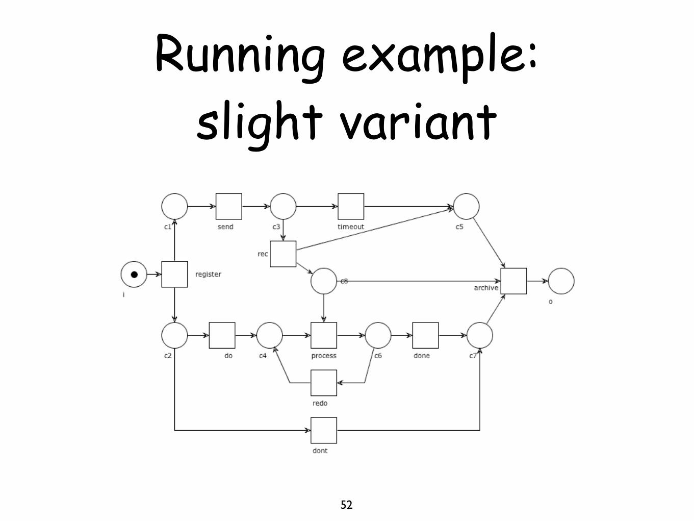
Running example: slight variant
52
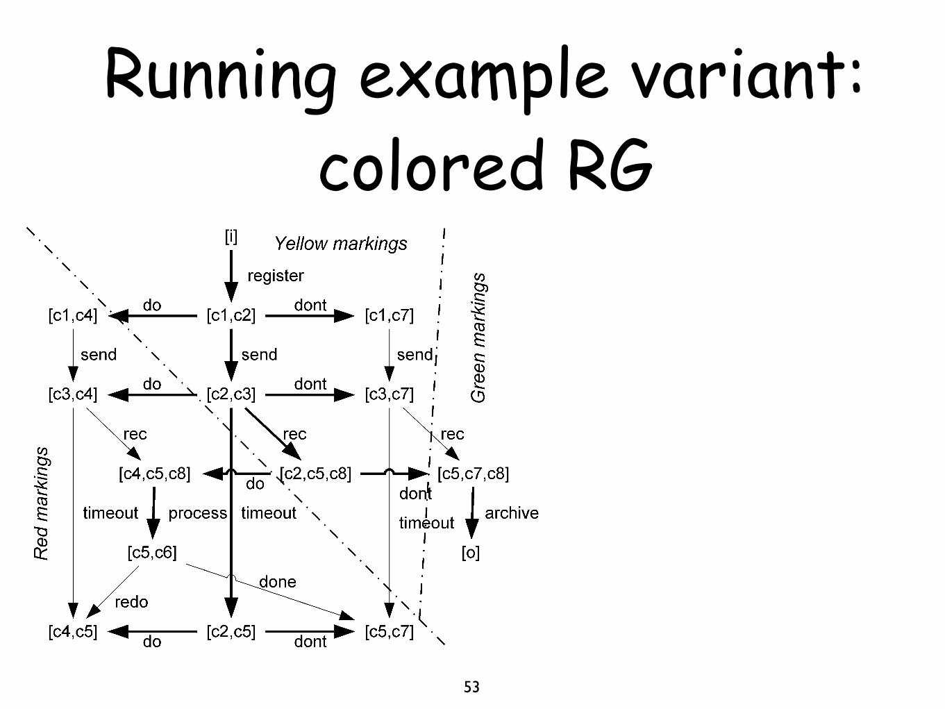
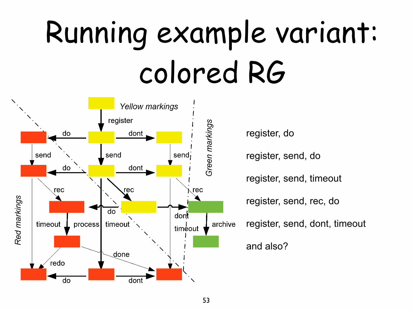
Running example variant: colored RG
53
DIAGNOSING WORKFLOW PROCESSES USING WOFLAN 17
iff Mn ⇥ HR and Mn�1 ⇥ HY . A firing sequence of a WF
system is called non-live iff it is derived from a non-live oc-
currence sequence.
The most valuable information in a non-live sequence is
the combination of its last two markings (Mn�1 ⇥ HY and
Mn ⇥ HR) and its last transition (tn�1). The only interestwe have in the sequence’s prefix ([i]t0M1 . . . tn�2) is that itgives us a path which leads to the last-but-one marking. Note
that we have excluded firing sequences containing cycles (by
requiring that all markings in a non-live sequence must be
distinct); cycles do not provide any additional useful infor-
mation. Also note that it is possible that several non-live
sequences have the same suffix Mn�1tn�1Mn .
THEOREM 4.10. (Non-live sequences vs. liveness) Let S
be a WF system without dead transitions such that the short-
circuited system S is bounded. Then, S is live iff S has no
non-live sequences.
Proof. The theorem follows immediately from Theorem 4.9
(Liveness of bounded short-circuited WF systems) and Def-
inition 4.5 (Non-live sequences).
Note that, based on Theorem 4.1, Theorem 4.10 can alter-
natively be formulated as follows. If S = (N , [i]) is a WF
system without dead transitions such that the short-circuited
system S is bounded, then N is sound iff S has no non-live
sequences.
FIGURE 12. WF net N1
As an example, consider the WF net N1 of Figure 12. It
is a variant of WF net N of Figure 1 with an extra arc from
place c8 to transition archive. The OG of S1=(N1, [i])
is shown in Figure 13. The meaning of the thick arcs is ex-
plained in the next section. Clearly, S1 has no dead tran-
sitions. Since the OG of S1=(N1, [i]) is simply the graph
in Figure 13 extended with the arc ([o], shortcircuit,
[i]), where shortcircuit is the short-circuiting transi-
tion, we see that S1 is bounded. Figure 13 also shows the
partitioning of the OG of S1 according to Definition 4.4. We
FIGURE 13. The OG of S1 partitioned for non-live sequences
can deduce, among others, the following five non-live se-
quences:
(i). register send timeout,
(ii). register send dont timeout,
(iii). register send rec do,
(iv). register send do, and
(v). register do.
Since S1 has non-live sequences, we can deduce from The-
orem 4.10 that S1 is not live, which means that N1 is not
sound. It is also possible to arrive at this conclusion by in-
vestigating the OG of S1. Since it contains deadlock mark-
ing [c4,c5], it follows that all transitions of S1 are non-live.
Unfortunately, the information that all transitions are non-
live is not sufficiently specific to be useful. By examining
the above five non-live sequences, we can obtain more de-
tailed information. Note that non-live sequence (ii) provides
almost the same information as sequence (i). Together, they
show that the combination send and timeout is the pos-
sible cause of an error and that dont is not important. From
sequence (i), we conclude that, whatever happens, place c8
does not get a token. As a result, transitions process and
archive cannot fire. The sequences (iii), (iv), and (v) pro-
vide the information that firing transition do always results
in an error. We may conclude that the cycle to which do
leads might cause a problem. For now, we do not go into
details about possible solutions to correct the errors.
4.4.5. Unbounded sequences
Intuitively, an unbounded sequence is a firing sequence of a
WF system of minimal length such that every continuation
implies a violation of the proper-completion requirement of
Definition 4.2. Such a violation can have two causes. The
first one is the most straightforward one. Clearly, proper
completion is violated if a reachable marking is strictly
greater than the marking [o] that signals proper completion.
The second cause is more implicit. If a WF system is un-
bounded, then the proper-completion requirement is also vi-
THE COMPUTER JOURNAL, Vol. ??, No. ??, ????
register, do
register, send, do
register, send, timeout
register, send, rec, do
register, send, dont, timeout
and also?
Unbounded sequences: informally
55
An unbounded sequence is a firing sequence of minimal length such that
every continuation leads to invalidate proper completion
i.e. a witness for unboundedness
Unbounded sequences: fundamental property
56
N* is bounded iff
N has no unbounded sequences
Undesired markings: infinite-weighted markings or markings greater than o
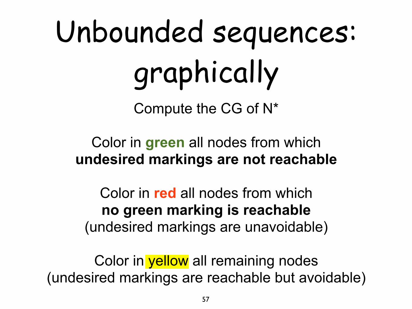
Unbounded sequences: graphically
57
Compute the CG of N*
Color in green all nodes from which undesired markings are not reachable
Color in red all nodes from which no green marking is reachable
(undesired markings are unavoidable)
Color in yellow all remaining nodes (undesired markings are reachable but avoidable)
Unbounded sequences: remarks
58
No red node implies no yellow node
No green node implies no yellow node
Restricted coverability graph (RCG)
59
CG can become very large (intractable!)
Basic observation: infinite-weighted markings leads to infinite-weighted markings
and they will be all red
We can just avoid computing them!
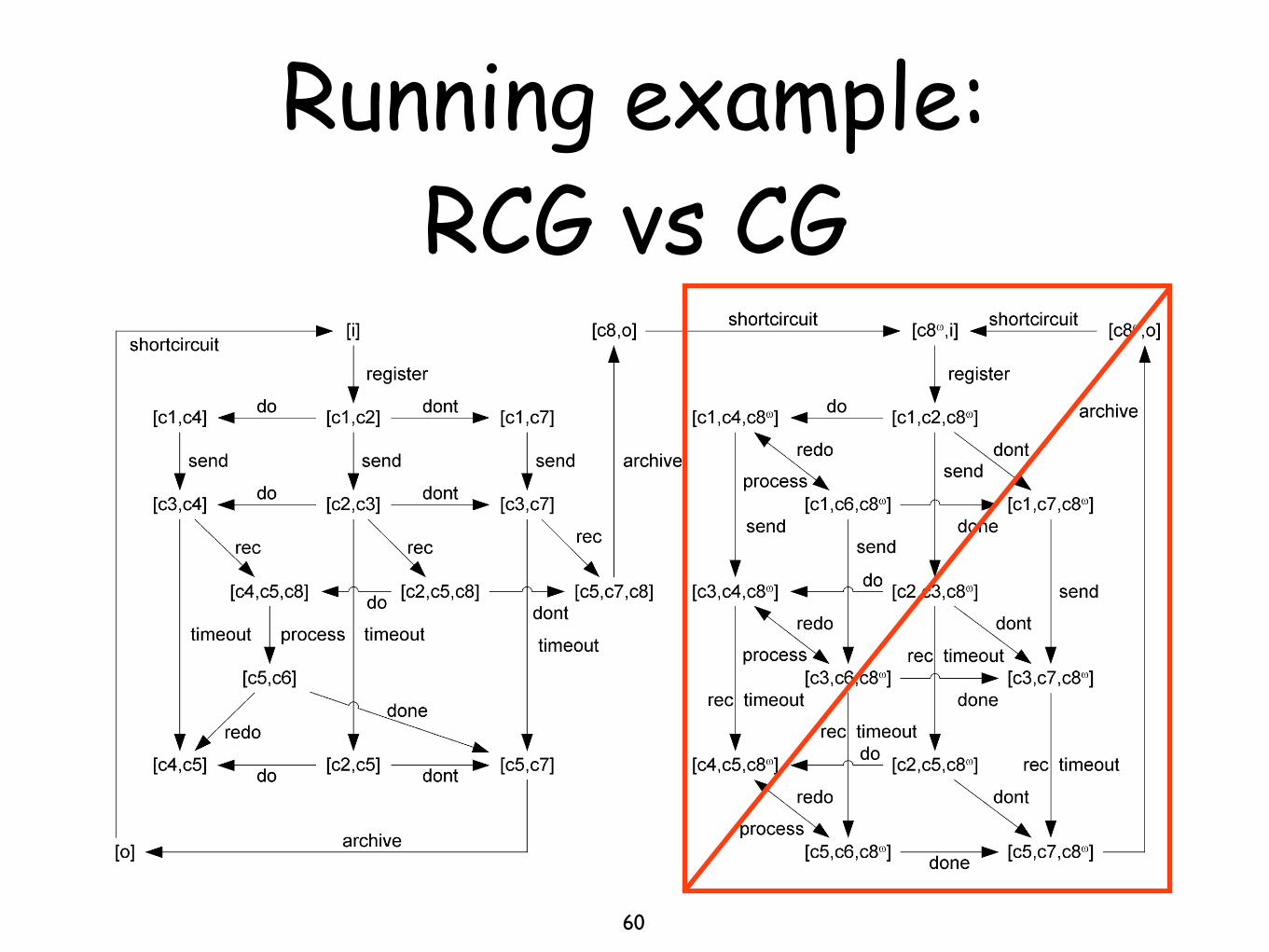
Running example: RCG vs CG
60
8 H. VERBEEK, T. BASTEN AND W. VAN DER AALST
FIGURE 8. The CG for the short-circuited system S
workflow processes. Cases are often generated by an exter-
nal customer. However, it is also possible that a case is gen-
erated by another department within the same organization
(internal customer). A typical example of a process that is
not case-based, and hence not a workflow process, is a pro-
duction process such as the assembly of bicycles. The task
of putting a tire on a wheel is (generally) independent of the
specific bicycle for which the wheel will be used. Note that
the production of bicycles to order, i.e., procurement, pro-
duction, and assembly are driven by individual orders, can
be considered as a workflow process.
The goal of workflow management is to handle cases as
efficient and effective as possible. A workflow process is
designed to handle large numbers of similar cases. Handling
one customer complaint usually does not differ much from
handling another customer complaint. The basis of a work-
flow process is the workflow process definition. This process
definition specifies which tasks need to be executed in what
order. Alternative terms for workflow process definition are:
‘procedure’, ‘workflow schema’, ‘flow diagram’, and ‘rout-
ing definition’. Tasks are ordered by specifying for each task
the conditions that need to be fulfilled before it may be ex-
ecuted. In addition, it is specified which conditions are ful-
filled by executing a specific task. Thus, a partial ordering of
tasks is obtained. In a workflow process definition, standard
routing elements are used to describe sequential, alternative,
parallel, and iterative routing thus specifying the appropri-
ate route of a case. The workflow management coalition
(WfMC) has standardized a few basic building blocks for
constructing workflow process definitions [29]. A so-called
OR-split is used to specify a choice between several alter-
natives; an OR-join specifies that several alternatives in the
workflow process definition come together. An AND-split
and an AND-join can be used to specify the beginning and
the end of parallel branches in the workflow process defini-
tion. The routing decisions in OR-splits are often based on
data such as the age of a customer, the department responsi-
ble, or the contents of a letter from the customer.
Many cases can be handled by following the same work-
flow process definition. As a result, the same task has to
be executed for many cases. A task that needs to be exe-
cuted for a specific case is called a work item. An example
of a work item is the order to execute task ‘send refund form
to customer’ for case ‘complaint of customer Baker’. Most
work items need a resource in order to be executed. A re-
source is either a machine (e.g., a printer or a fax) or a per-
son (participant, worker, or employee). Besides a resource,
a work item often needs a trigger. A trigger specifies who
or what initiates the execution of a work item. Often, the
trigger for a work item is the resource that must execute the
work item. Other common triggers are external triggers and
time triggers. An example of an external trigger is an incom-
ing phone call of a customer; an example of a time trigger is
the expiration of a deadline. A work item that is being ex-
ecuted is called an activity. If we take a photograph of the
state of a workflow, we see cases, work items, and activities.
Work items link cases and tasks. Activities link cases, tasks,
triggers, and resources.
A thorough investigation of the business processes in a
company that results in a complete set of efficient and ef-
fective workflow processes is the basis of the successful in-
troduction of a workflow system. Formal (qualitative and
quantitative) verification can be a useful aid in obtaining the
desired effectiveness and efficiency.
3.2. Workflow perspectives and abstraction
In the previous subsection, we introduced the workflow con-
cepts used in the remainder of this paper. Workflow man-
agement has many aspects and typically involves many dis-
ciplines. The verification tool presented in this paper fo-
THE COMPUTER JOURNAL, Vol. ??, No. ??, ????
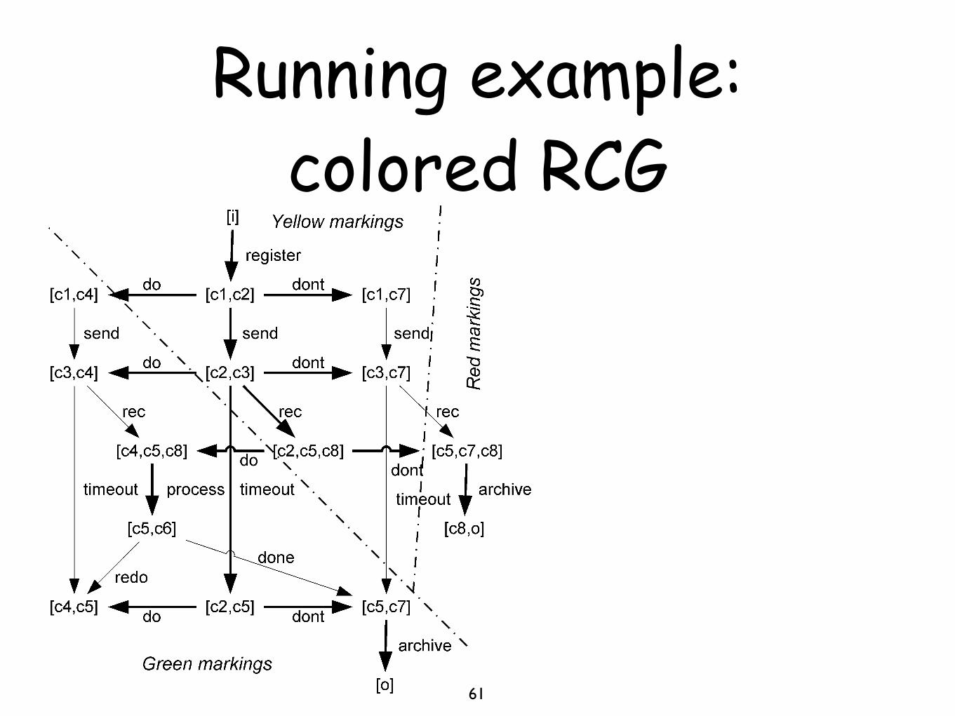
DIAGNOSING WORKFLOW PROCESSES USING WOFLAN 19
Figure 3 depicted in Figure 8 with the RCG of Figure 14.
For this simple example, the RCG is approximately half the
size of the CG. Note that if a system is bounded the RCG-
generation algorithm and the CG-generation algorithm both
yield the OG of the system.
FIGURE 14. The RCG of the short-circuited example net
It is straightforward to see that an RCG can be used to
compute the unbounded sequences of a WF system. Con-
sider the partitioning of a CG given in Definition 4.6. Since
infinite markings are always red, it is clear that successors of
infinite markings are also red. Therefore, the part of a CG
that is omitted in an RCG is not used when constructing un-
bounded sequences. This means that unbounded sequences
can be computed by applying the partitioning of Definition
4.6 to an RCG.
The idea to restrict a CG of a system to an RCG is similar
to one of the ideas behind the notion of an MCG (minimal
CG) of [21]. In general, an RCG of a system is still larger
than its MCG. Unfortunately, the MCG of a WF system is
not suitable for computing unbounded sequences. For more
details, the interested reader is referred to [21].
Figure 15 shows the partitioned RCG of the example sys-
tem S of Figure 2. Note that this RCG is the OG of S, be-
cause S is bounded. S has among others the following un-
bounded sequences:
(i). register send rec dont and
(ii). register send dont rec.
These two sequences show that firing the combination of
rec and dont inevitably leads to unboundedness of the
short-circuited system. The reason is that rec puts a to-
ken in place c8, whereas firing dont removes the option to
remove this token via transition process.
5. WOFLAN
This section describes Woflan (WOrkFLow ANalyzer, see
http://www.tm.tue.nl/it/woflan) version 2.1. Woflan is a tool
FIGURE 15. The RCG partitioned for unboundedness
that analyzes workflow process definitions specified in terms
of Petri nets. It has been designed to verify process defi-
nitions that are downloaded from a workflow management
system, as explained in Section 3.3. As indicated in the in-
troduction, there is a clear need for such a verification tool.
Based on some of the results presented in the previous sec-
tion, the development of the tool Woflan started at the end of
1996 and the first version was released in 1997 [8]. Basi-
cally, Woflan takes a workflow process definition imported
from some workflow product, translates it into a P/T net, and
tells whether or not the net is a sound WF net. Furthermore,
using some standard P/T net-analysis techniques as well as
those tailored to WF nets presented in the previous section,
the tool provides diagnostic information about the net in case
it is not a soundWF net. Woflan implements a predefined di-
agnosis process illustrated in Figure 16. The diagnosis pro-
cess is in fact a workflow process modeled in Protos [31]. In
the next subsection, the diagnosis process of Figure 16 is ex-
plained in detail. In Section 5.2, the P/T net of Figure 1 is
analyzed by means ofWoflan. Version 2.1 ofWoflan extends
version 1.0 as described in [8] with some new analysis tech-
niques of which the technique of behavioral error sequences
is the most important one, with a predefined, detailed diag-
nosis process that uses a new, workflow-oriented nomencla-
ture, and with an import facility for COSA, Staffware, ME-
TEOR, and Protos. A brief overview of the material of this
section was presented at the 2000 International Conference
on Application and Theory of Petri nets [45].
5.1. Diagnosis process
In Sections 2 and 4, we have seen a wide range of analysis
techniques for P/T nets in general and WF nets in particu-
lar. The goal is to apply these techniques in the analysis of
workflow processes in a logical and meaningful order, and
to distill useful diagnostic information from the analysis re-
sults in case of errors in the workflow. The diagnosis process
THE COMPUTER JOURNAL, Vol. ??, No. ??, ????
Running example: colored RCG
61
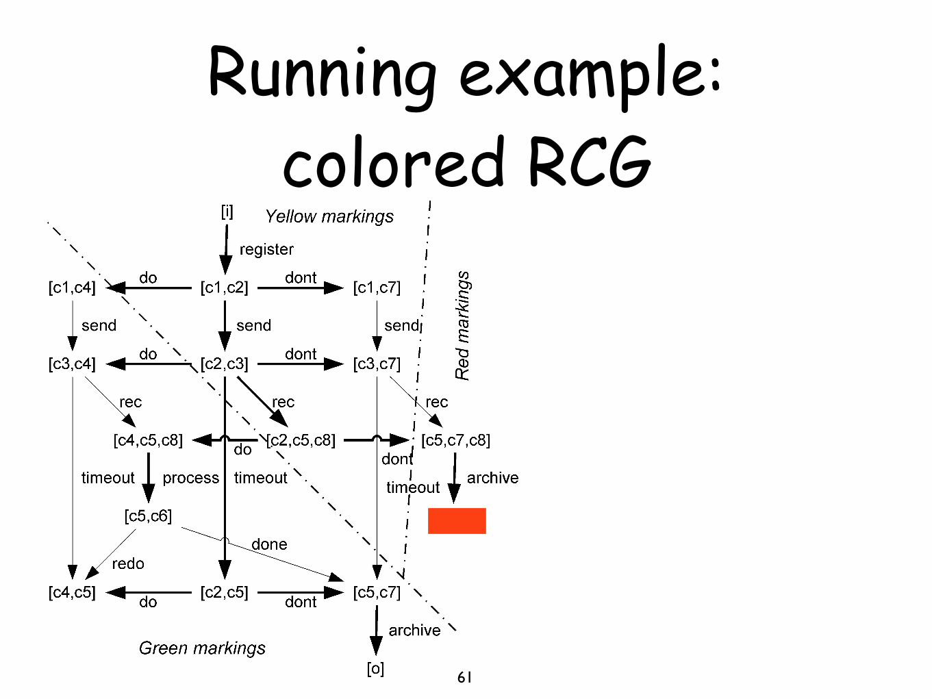
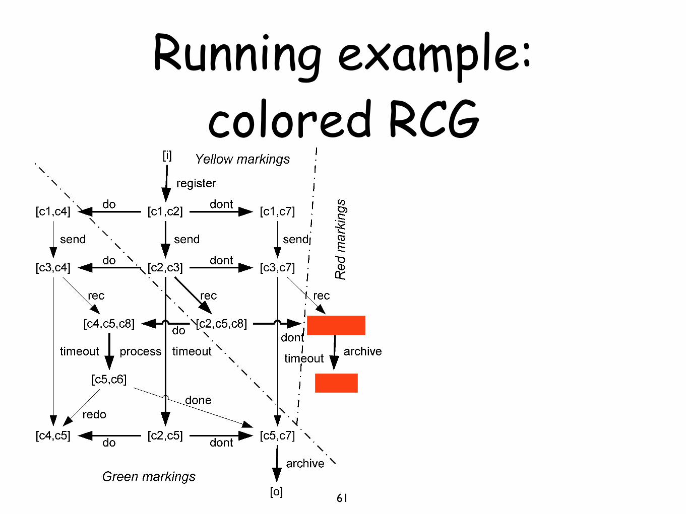
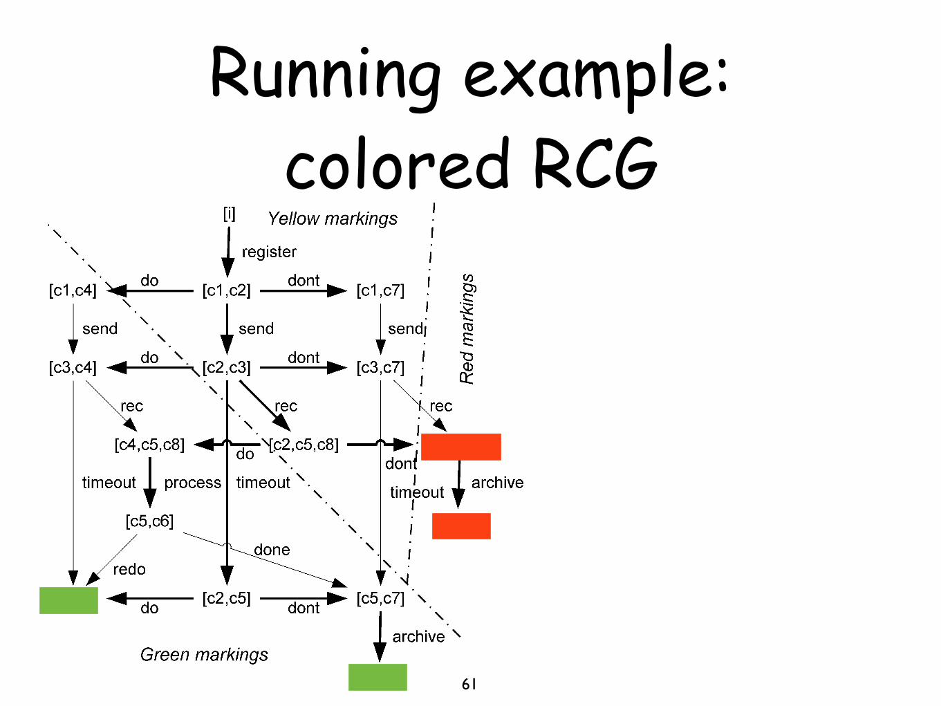
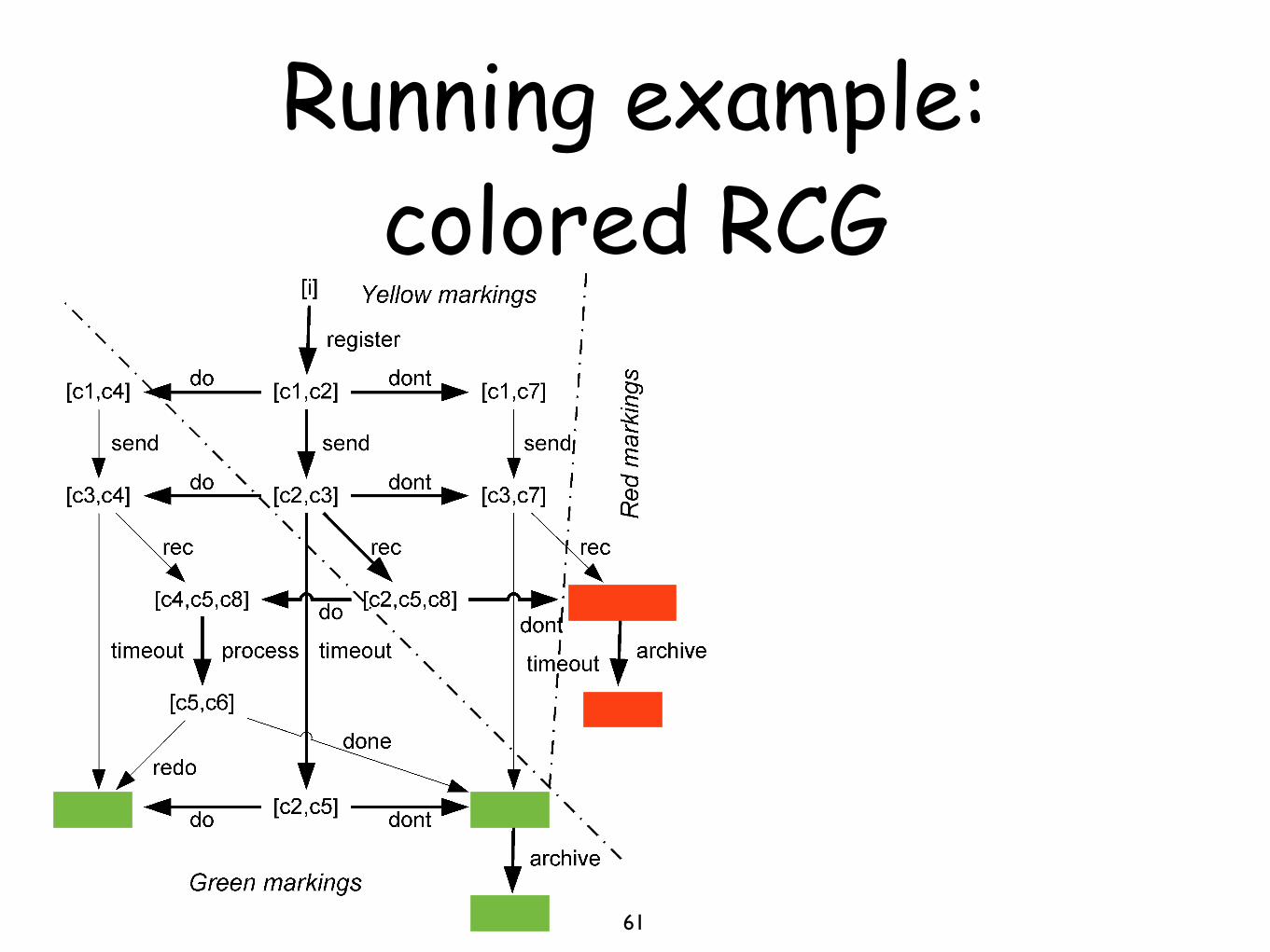
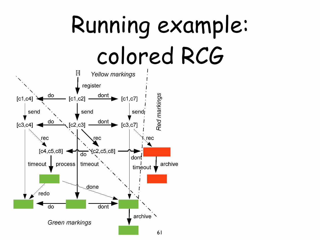
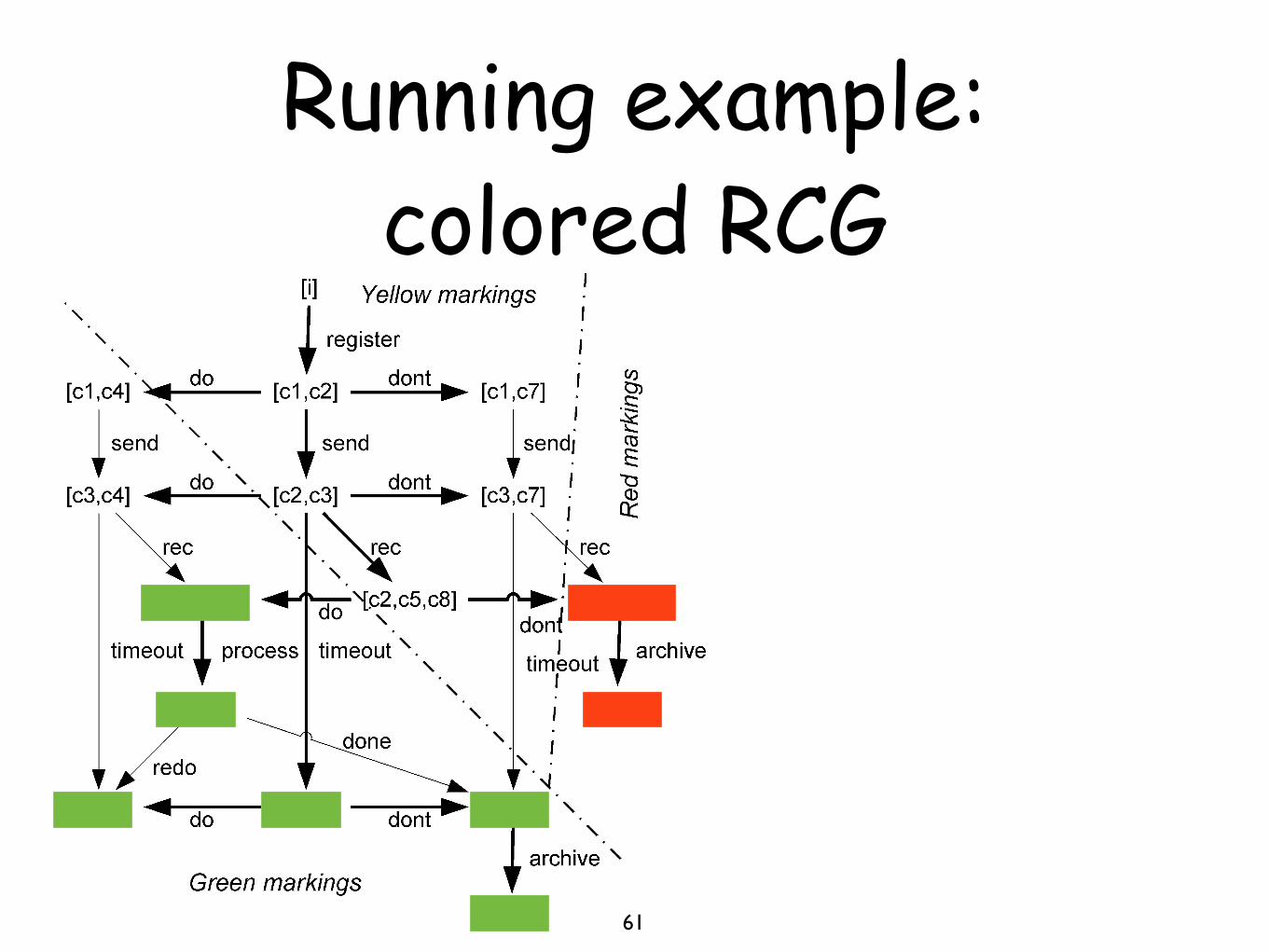
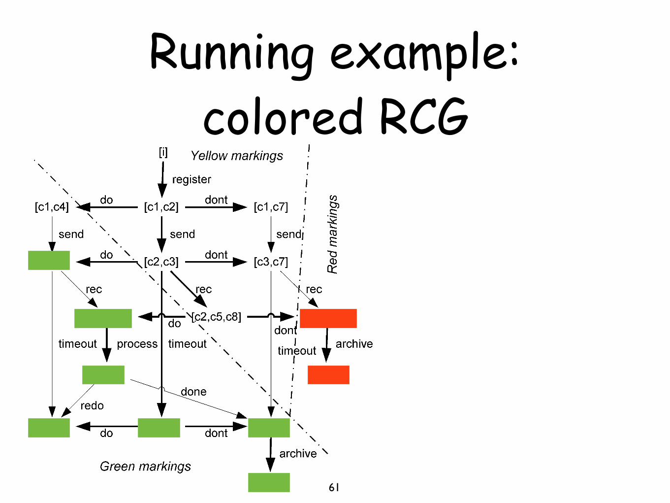
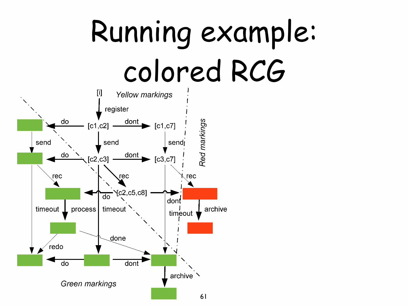
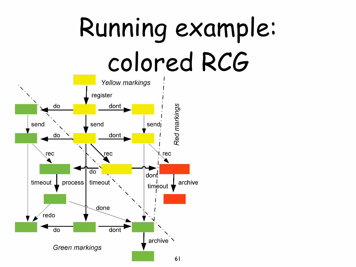
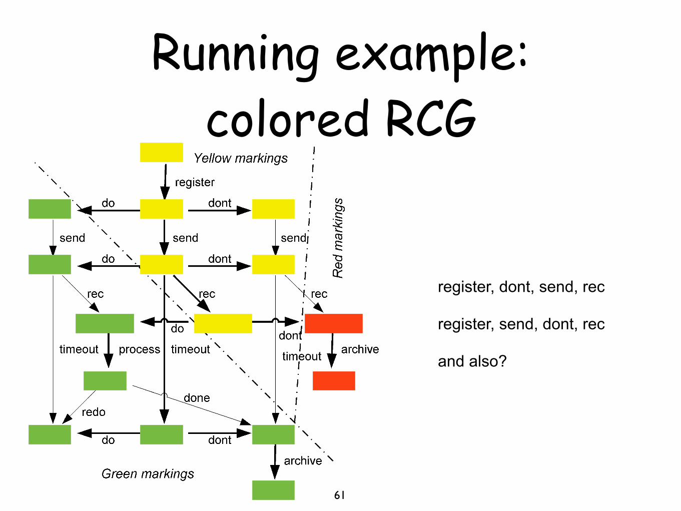
register, dont, send, rec
register, send, dont, rec
and also?
Practice with WoPeD (and Woflan)
63
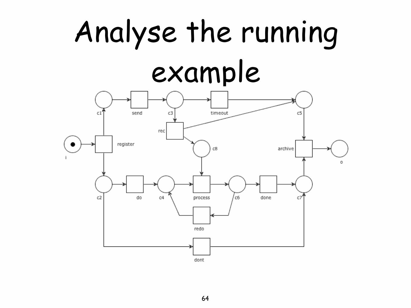
Analyse the running example
64
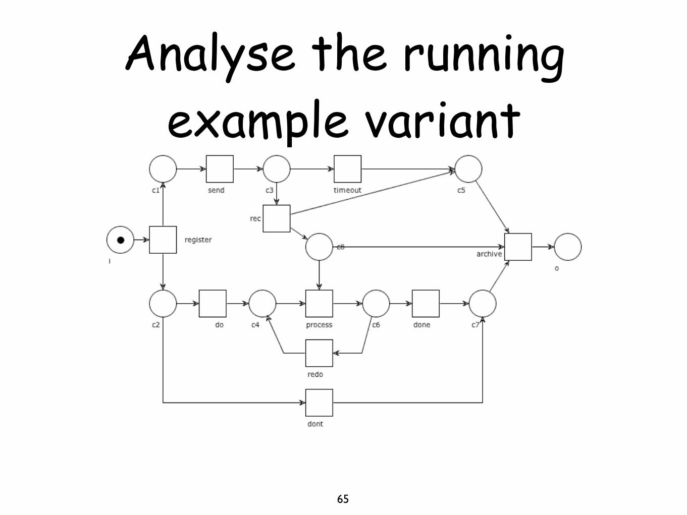
Analyse the running example variant
65
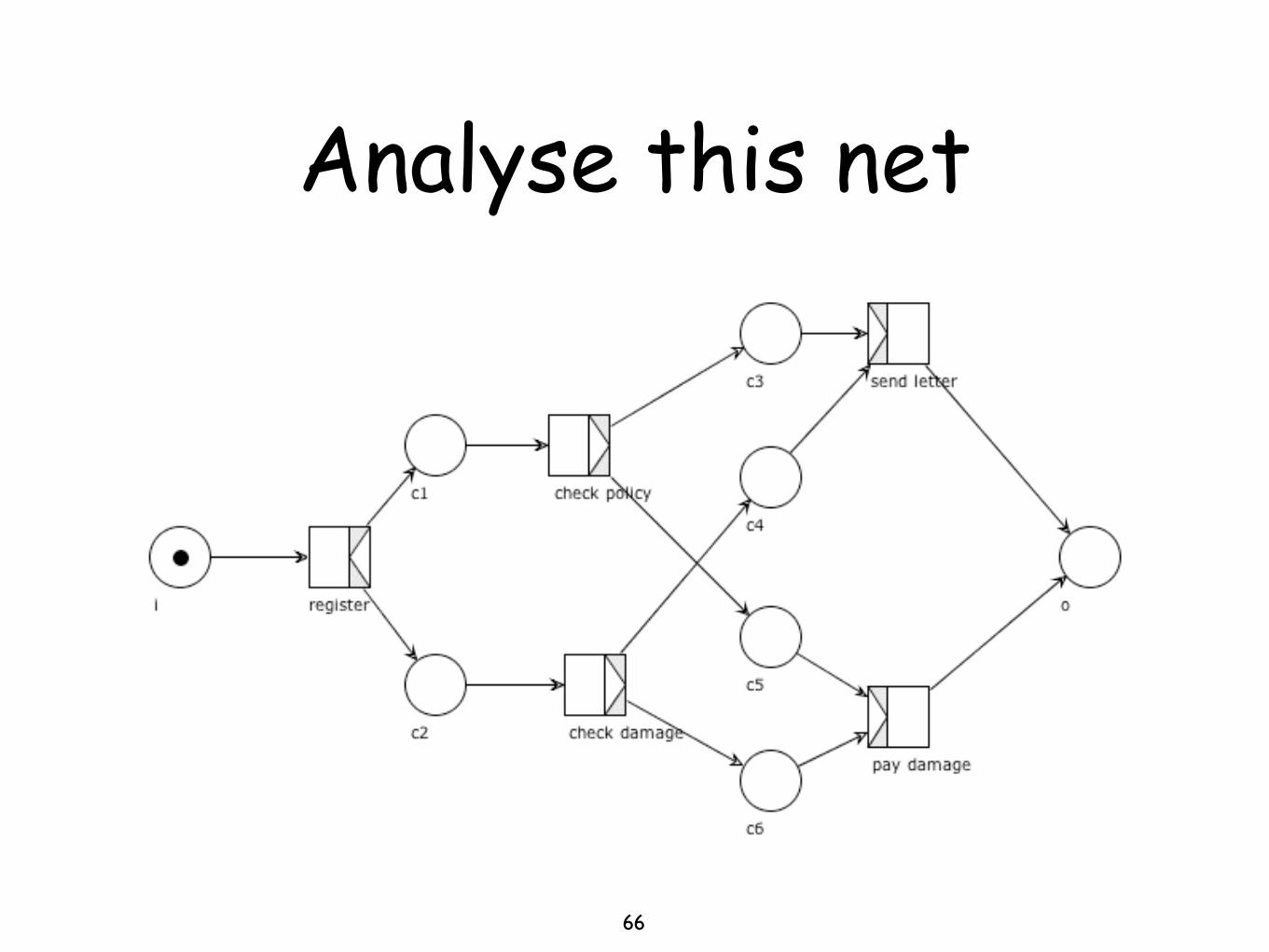
Analyse this net
66
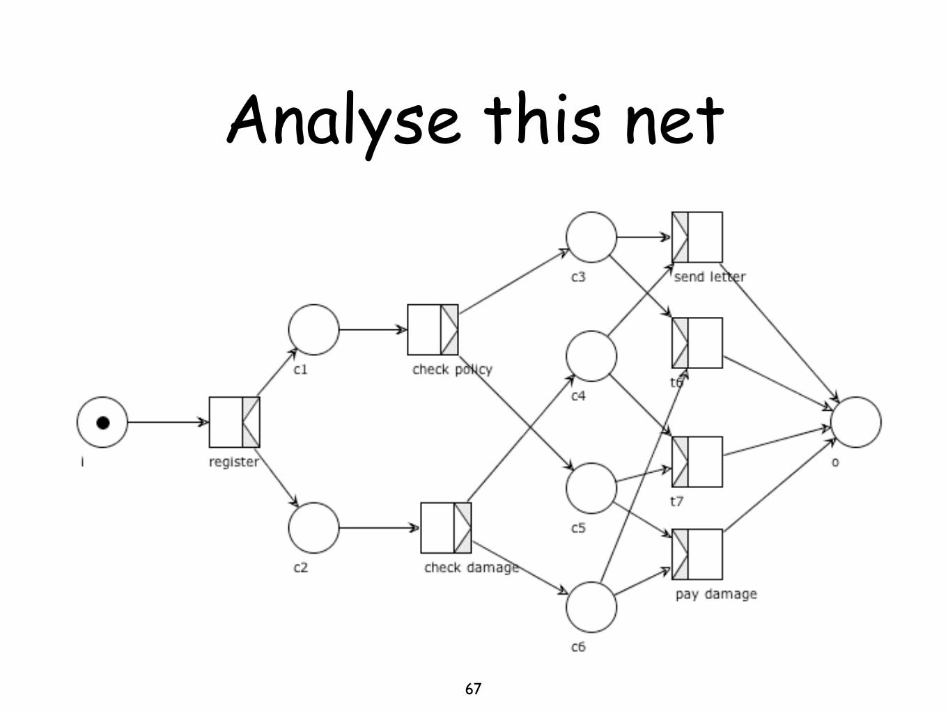
Analyse this net
67
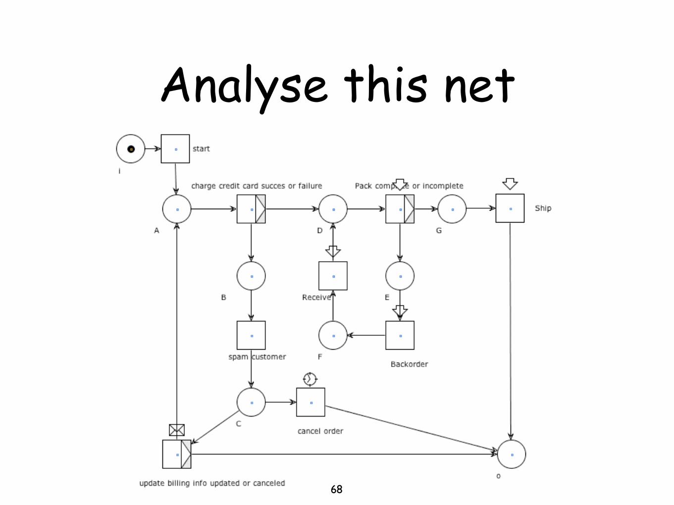
Analyse this net
68
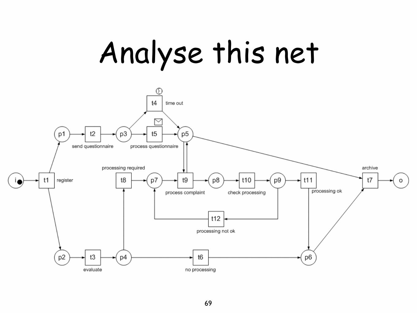
Analyse this net
69
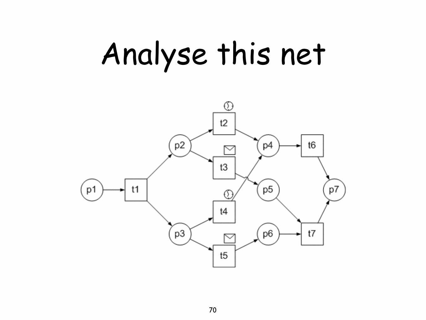
Analyse this net
70
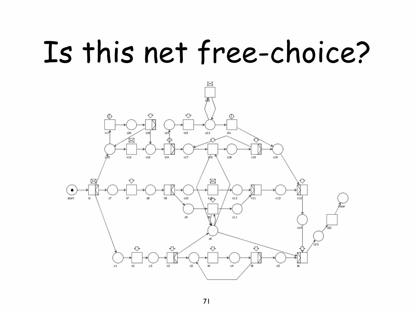
Is this net free-choice?
71
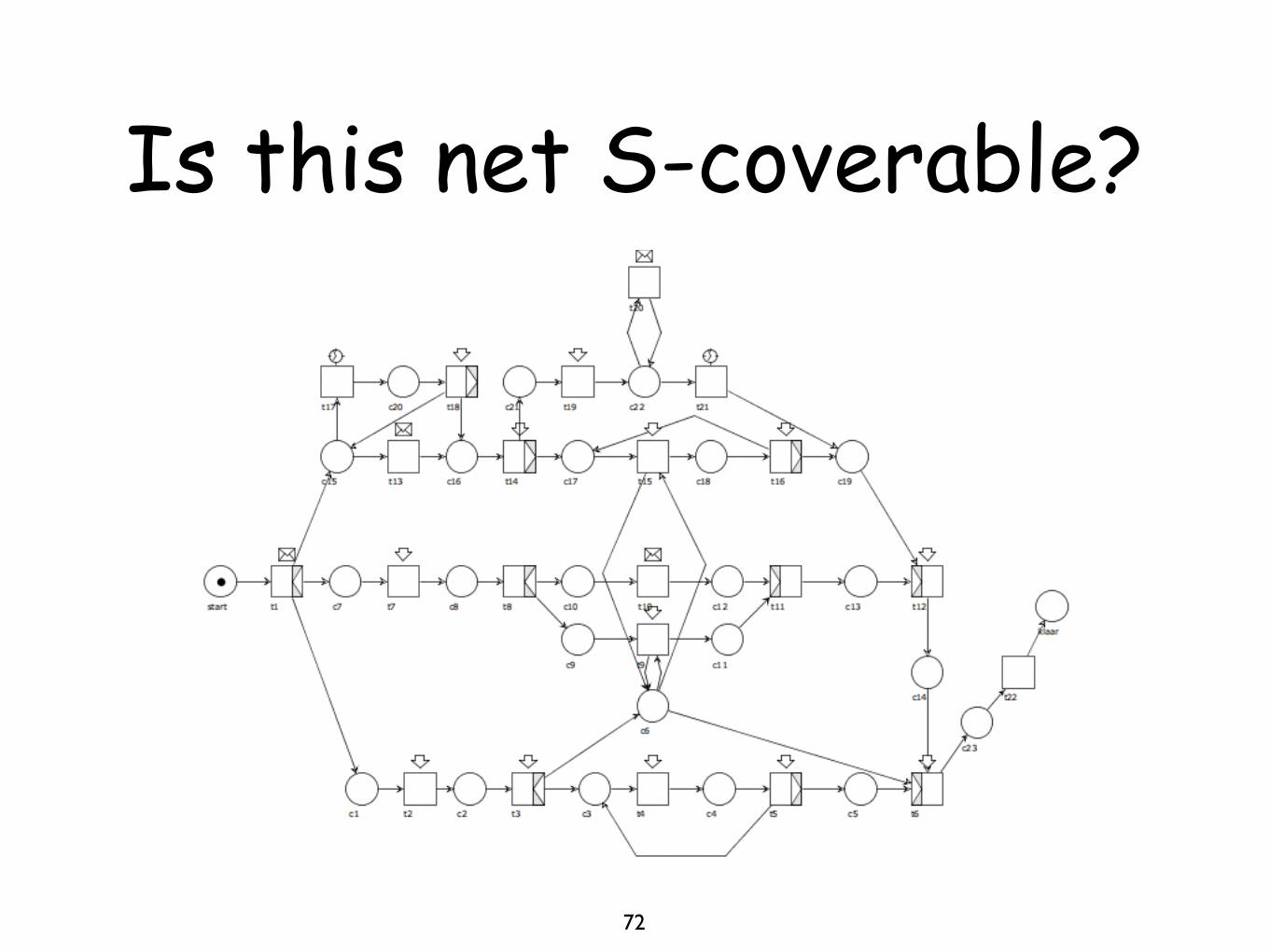
Is this net S-coverable?
72
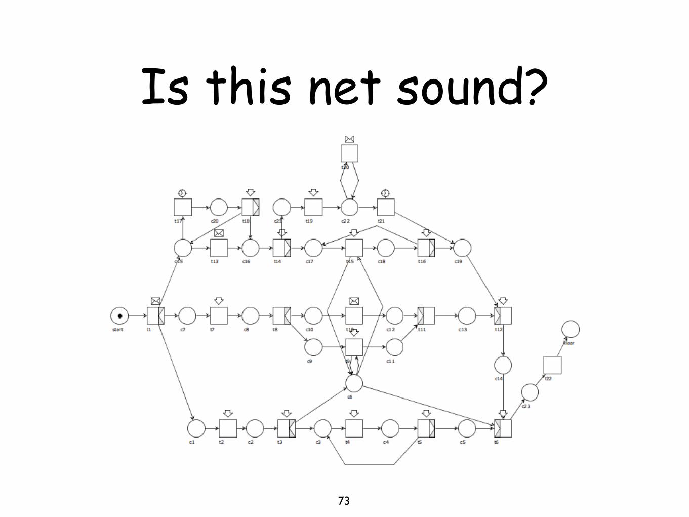
Is this net sound?
73
Design and analysis of WF-nets
74
The workflow of a computer repair service (CRS) can be described as follows. A customer brings in a defective computer and the CRS checks the defect and hands out a repair cost calculation back. If the customer decides that the costs are acceptable, the process continues, otherwise she takes her computer home unrepaired. The ongoing repair consists of two activities, which are executed, in an arbitrary order. The first activity is to check and repair the hardware, whereas the second activity checks and configures the software. After each of these activities, the proper system functionality is tested. If an error is detected another arbitrary repair activity is executed, otherwise the repair is finished.
Model the described workflow as a sound workflow net.

Design and analysis of WF-nets
75
A hospital wants to establish a rating workflow for their doctors. To make the workflow reliable two different roles are assigned. The first one is a referee from the newly created quality assurance department while the second one represents the managing director of the hospital. Both roles execute all of their tasks independently from each other.
The referee starts a new case regarding a certain doctor by interviewing patients. Since a patient interview workflow is already established, it is simply integrated in the new workflow. Meanwhile, the director asks an external expert to review the work of the doctor under rating. Unfortunately, since the expert only gets a low expenses fee, it can happen that the expert is not responding in time. If that happens, another expert has to be asked (who could also not respond in time, i.e. the procedure repeats). If an expert finally sends an expertise, it is received by the director and forwarded to the referee. The referee files the results containing the patient interviews as well as the expertise and afterward creates a report. While the referee is doing this, the manager fills a cheque to pay the expenses of the expert.
Model the described workflow as a sound workflow net.