UNCERTAINTIES IN LCA

Methods for global sensitivity analysis in life cycle assessment

Evelyne A. Groen1& Eddie A. M. Bokkers1 & Reinout Heijungs2,3 & Imke J. M. de Boer1

Received: 9 April 2015 /Accepted: 25 October 2016 /Published online: 28 November 2016# The Author(s) 2016. This article is published with open access at Springerlink.com

AbstractPurpose Input parameters required to quantify environmentalimpact in life cycle assessment (LCA) can be uncertain due toe.g. temporal variability or unknowns about the true value ofemission factors. Uncertainty of environmental impact can beanalysed by means of a global sensitivity analysis to gainmore insight into output variance. This study aimed to (1) giveinsight into and (2) compare methods for global sensitivityanalysis in life cycle assessment, with a focus on the inventorystage.Methods Five methods that quantify the contribution to out-put variance were evaluated: squared standardized regressioncoefficient, squared Spearman correlation coefficient, key is-sue analysis, Sobol’ indices and random balance design. To beable to compare the performance of global sensitivitymethods, two case studies were constructed: one small hypo-thetical case study describing electricity production that is

sensitive to a small change in the input parameters and a largecase study describing a production system of a northeastAtlantic fishery. Input parameters with relative small and largeinput uncertainties were constructed. The comparison of thesensitivity methods was based on four aspects: (I) samplingdesign, (II) output variance, (III) explained variance and (IV)contribution to output variance of individual input parameters.Results and discussion The evaluation of the sampling design(I) relates to the computational effort of a sensitivity method.Key issue analysis does not make use of sampling and wasfastest, whereas the Sobol’ method had to generate two sam-pling matrices and, therefore, was slowest. The total outputvariance (II) resulted in approximately the same output vari-ance for each method, except for key issue analysis, whichunderestimated the variance especially for high input uncer-tainties. The explained variance (III) and contribution to var-iance (IV) for small input uncertainties were optimally quan-tified by the squared standardized regression coefficients andthe main Sobol’ index. For large input uncertainties,Spearman correlation coefficients and the Sobol’ indices per-formed best. The comparison, however, was based on twocase studies only.Conclusions Most methods for global sensitivity analysis per-formed equally well, especially for relatively small input un-certainties. When restricted to the assumptions that quantifi-cation of environmental impact in LCAs behaves linearly,squared standardized regression coefficients, squaredSpearman correlation coefficients, Sobol’ indices or key issueanalysis can be used for global sensitivity analysis. The choicefor one of the methods depends on the available data, themagnitude of the uncertainties of data and the aim of the study.

Keywords Correlation .Key issue analysis .Randombalancedesign . Regression . Sensitivity analysis . Sobol’ sensitivityindex . Variance decomposition

Responsible editor: Walter Klöpffer

Electronic supplementary material The online version of this article(doi:10.1007/s11367-016-1217-3) contains supplementary material,which is available to authorized users.

* Evelyne A. Groenevelyne.groen@gmail.com

1 Animal Production Systems Group,Wageningen University, POBox338, 6700 AH Wageningen, the Netherlands

2 Institute of Environmental Sciences, Leiden University, PO Box9518, 2300 RA Leiden, the Netherlands

3 Department of Econometrics and Operations Research, VUUniversity Amsterdam, De Boelelaan 1105, 1081HVAmsterdam, the Netherlands

Int J Life Cycle Assess (2017) 22:1125–1137DOI 10.1007/s11367-016-1217-3

1 Introduction

Life cycle assessment (LCA) calculates the environmental im-pact of a product or production process along the entire chain.Input parameters required to describe the production chain canbe uncertain due to e.g. temporal variability or unknownsabout the true value of emission factors. Uncertainty in theinput parameters will cause an uncertainty around the outcomeof an LCA. In this paper, uncertainty can refer to variability orepistemic uncertainty (Chen and Corson 2014; Clavreul et al.2013) of the input parameters. Variability (e.g. natural, tem-poral, geographical) is inherent to natural systems and cannotbe reduced. Epistemic uncertainty refers to unknowns in thesystem and can be reduced by gaining more knowledge aboutthe system. Analysing this uncertainty can be done by meansof a sensitivity analysis and can help to gain more insight intothe robustness of the result, to prioritize data collection or tosimplify an LCA model. Many LCA studies have been per-formed over the last decade, and interest in addressing uncer-tainty propagation is increasing (Groen et al. 2014; Heijungsand Lenzen 2014; Lloyd and Ries 2007). However, few stud-ies apply a systematic sensitivity analysis to address the effectof input uncertainties on the output (Mutel et al. 2013). Anexplanation might be that ISO 14044 recommends a sensitiv-ity analysis as part of the LCA framework to identify theimportance of the input uncertainties, but does not recommenda specific technique.

A sensitivity analysis can be performed by varying an inputparameter and, as such, determining the effect on the result.Furthermore, if the distribution function of the input parame-ters is known, it is possible to calculate the contribution to theoutput variance. The first approach belongs to the area of localsensitivity analysis. A local sensitivity analysis determines theeffect of a (small) change in one of the input parameters at atime. The second approach belongs to the area of global sen-sitivity analysis. A global sensitivity analysis can be seen as anextension of uncertainty propagation: it determines howmucheach input parameter contributes to the output variance. Whilewe acknowledge that GSA can be done in several ways, e.g.by density-based methods (Borgonovo and Pliscke 2016), wefocus in this article onmethods that address the contribution tovariance (CTV, see Saltelli et al. 2008) and not e.g. onmoment-independent methods (as used by Cucurachi 2014).The main differences between a local and global sensitivityanalysis are illustrated in Table 1. In this paper, we focus onglobal sensitivity analysis, which requires a case study ofwhich the distribution functions of the input parameters areknown.

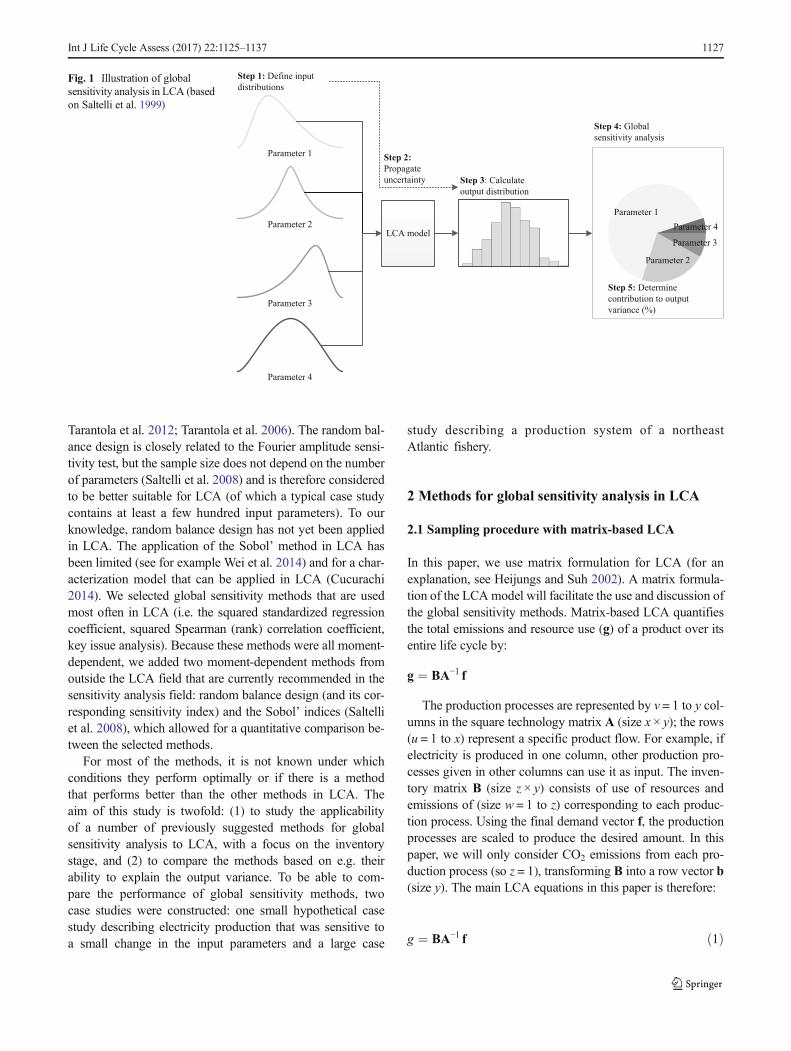
In Fig. 1, the procedure of a global sensitivity analysis isillustrated with a schematic LCAmodel, containing four inputparameters. First, the input parameters and their uncertaintiesare represented by probability density functions (step 1).Second, uncertainty propagation is performed with e.g.

Monte Carlo simulation, which propagates uncertaintythrough the LCA model (step 2) to obtain a distribution func-tion of the output. Third, the variance of the output is calcu-lated (step 3). After the uncertainty propagation is performed,a method for global sensitivity analysis is selected (step 4),which determines howmuch each input parameter contributesto the output variance (step 5). In the example of Fig. 1, thesensitivity analysis shows that parameter 1 and to a lesserextent parameter 2 are the ones that contribute most to theoutput variance.

In LCA literature, five methods for global sensitivity anal-ysis have been mentioned that quantify the contribution tooutput variance: (1) (squared standardized) regression coeffi-cients, as was suggested by Huijbregts et al. (2001) and ap-plied in LCA by e.g. Aktas and Bilec (2012), Basset-Menset al. (2009), Sugiyama et al. (2005) and Vigne et al. (2012);(2) (squared) Pearson correlation coefficient (Heijungs andLenzen 2014; Onat et al. 2014); (3) (squared) Spearman(rank) correlation coefficient (Chen and Corson 2014;Geisler et al. 2005; Heijungs and Lenzen 2014; Mattila et al.2012; Mattinen et al. 2014; Sonnemann et al. 2003; Wang andShen 2013); (4) key issue analysis, which applies a first-orderTaylor expansion around the LCA model to estimate the out-put variance, thus avoiding sampling; key issue analysis inLCA has been developed by Heijungs (1996) and applied inLCA by e.g. Heijungs et al. (2005) and Jung et al. (2014); and(5) Fourier amplitude sensitivity test has been applied by deKoning et al. (2010).

Outside the LCA domain, a much wider set of approacheshave been developed and applied, such as random balancedesign and the Sobol’method, that also quantify the contribu-tion to output variance (Saltelli et al. 2008; Sobol’ 2001;

Table 1 Main differences between local and global sensitivity analysis,described by differences in input data requirements and results

Local sensitivity analysis Global sensitivity analysis

Synonyms One at a time approach;differential analysis;marginal analysis;perturbation analysis

Contribution to variance;variance-based sensitivityanalysis; key issue analysis

Requirements Point value (central value) • Central value and parameterof dispersion

• Probability density function(depends on method)

• Uncertainty propagation

Result Ranking of (locally)sensitive input parame-ters

Contribution to outputvariance of each inputparameter; uncertaintydistribution of output;ranking

Examples Partial derivatives;(relative) change ofoutput due to change ofinput parameter

Regression or correlationtechniques; Sobol’ indices

1126 Int J Life Cycle Assess (2017) 22:1125–1137

Tarantola et al. 2012; Tarantola et al. 2006). The random bal-ance design is closely related to the Fourier amplitude sensi-tivity test, but the sample size does not depend on the numberof parameters (Saltelli et al. 2008) and is therefore consideredto be better suitable for LCA (of which a typical case studycontains at least a few hundred input parameters). To ourknowledge, random balance design has not yet been appliedin LCA. The application of the Sobol’ method in LCA hasbeen limited (see for example Wei et al. 2014) and for a char-acterization model that can be applied in LCA (Cucurachi2014). We selected global sensitivity methods that are usedmost often in LCA (i.e. the squared standardized regressioncoefficient, squared Spearman (rank) correlation coefficient,key issue analysis). Because these methods were all moment-dependent, we added two moment-dependent methods fromoutside the LCA field that are currently recommended in thesensitivity analysis field: random balance design (and its cor-responding sensitivity index) and the Sobol’ indices (Saltelliet al. 2008), which allowed for a quantitative comparison be-tween the selected methods.

For most of the methods, it is not known under whichconditions they perform optimally or if there is a methodthat performs better than the other methods in LCA. Theaim of this study is twofold: (1) to study the applicabilityof a number of previously suggested methods for globalsensitivity analysis to LCA, with a focus on the inventorystage, and (2) to compare the methods based on e.g. theirability to explain the output variance. To be able to com-pare the performance of global sensitivity methods, twocase studies were constructed: one small hypothetical casestudy describing electricity production that was sensitive toa small change in the input parameters and a large case

study describing a production system of a northeastAtlantic fishery.

2 Methods for global sensitivity analysis in LCA

2.1 Sampling procedure with matrix-based LCA

In this paper, we use matrix formulation for LCA (for anexplanation, see Heijungs and Suh 2002). A matrix formula-tion of the LCA model will facilitate the use and discussion ofthe global sensitivity methods. Matrix-based LCA quantifiesthe total emissions and resource use (g) of a product over itsentire life cycle by:

g ¼ BA−1 f

The production processes are represented by v = 1 to y col-umns in the square technology matrix A (size x × y); the rows(u = 1 to x) represent a specific product flow. For example, ifelectricity is produced in one column, other production pro-cesses given in other columns can use it as input. The inven-tory matrix B (size z × y) consists of use of resources andemissions of (size w = 1 to z) corresponding to each produc-tion process. Using the final demand vector f, the productionprocesses are scaled to produce the desired amount. In thispaper, we will only consider CO2 emissions from each pro-duction process (so z = 1), transforming B into a row vector b(size y). The main LCA equations in this paper is therefore:

g ¼ BA−1 f ð1Þ

Step 4: Global

sensitivity analysis

Parameter 1

Parameter 2

Parameter 3

LCA model

Step 1: Define input

distributions

Step 3: Calculate

output distribution

Parameter 4

Parameter 1

Parameter 4

Step 5: Determine

contribution to output

variance (%)

Parameter 2

Parameter 3

Step 2:

Propagate

uncertainty

Fig. 1 Illustration of globalsensitivity analysis in LCA (basedon Saltelli et al. 1999)

Int J Life Cycle Assess (2017) 22:1125–1137 1127

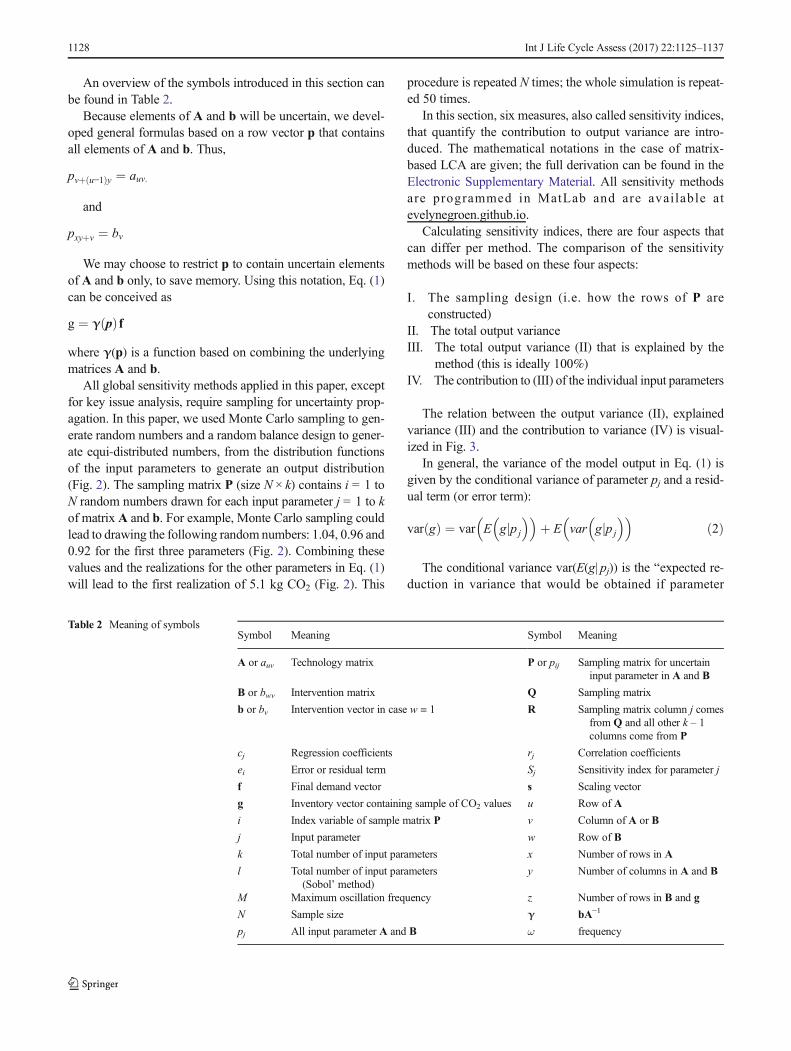
An overview of the symbols introduced in this section canbe found in Table 2.

Because elements of A and b will be uncertain, we devel-oped general formulas based on a row vector p that containsall elements of A and b. Thus,

pvþ u−1ð Þy ¼ auv:

and

pxyþv ¼ bv

We may choose to restrict p to contain uncertain elementsof A and b only, to save memory. Using this notation, Eq. (1)can be conceived as

g ¼ γ pð Þ f

where γ(p) is a function based on combining the underlyingmatrices A and b.

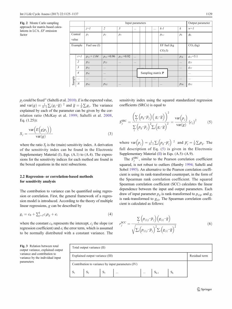
All global sensitivity methods applied in this paper, exceptfor key issue analysis, require sampling for uncertainty prop-agation. In this paper, we used Monte Carlo sampling to gen-erate random numbers and a random balance design to gener-ate equi-distributed numbers, from the distribution functionsof the input parameters to generate an output distribution(Fig. 2). The sampling matrix P (size N × k) contains i = 1 toN random numbers drawn for each input parameter j = 1 to kof matrix A and b. For example, Monte Carlo sampling couldlead to drawing the following random numbers: 1.04, 0.96 and0.92 for the first three parameters (Fig. 2). Combining thesevalues and the realizations for the other parameters in Eq. (1)will lead to the first realization of 5.1 kg CO2 (Fig. 2). This

procedure is repeated N times; the whole simulation is repeat-ed 50 times.

In this section, six measures, also called sensitivity indices,that quantify the contribution to output variance are intro-duced. The mathematical notations in the case of matrix-based LCA are given; the full derivation can be found in theElectronic Supplementary Material. All sensitivity methodsare programmed in MatLab and are available atevelynegroen.github.io.

Calculating sensitivity indices, there are four aspects thatcan differ per method. The comparison of the sensitivitymethods will be based on these four aspects:

I. The sampling design (i.e. how the rows of P areconstructed)

II. The total output varianceIII. The total output variance (II) that is explained by the

method (this is ideally 100%)IV. The contribution to (III) of the individual input parameters

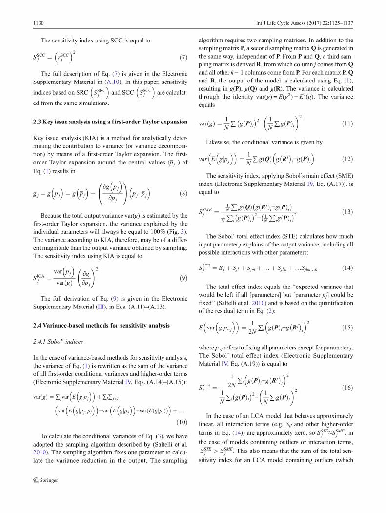
The relation between the output variance (II), explainedvariance (III) and the contribution to variance (IV) is visual-ized in Fig. 3.

In general, the variance of the model output in Eq. (1) isgiven by the conditional variance of parameter pj and a resid-ual term (or error term):

var gð Þ ¼ var E gjp j

� �� �þ E var gjpj

� �� �ð2Þ

The conditional variance var(E(g| pj)) is the Bexpected re-duction in variance that would be obtained if parameter

Table 2 Meaning of symbolsSymbol Meaning Symbol Meaning

A or auv Technology matrix P or pij Sampling matrix for uncertaininput parameter in A and B

B or bwv Intervention matrix Q Sampling matrix

b or bv Intervention vector in case w = 1 R Sampling matrix column j comesfrom Q and all other k – 1columns come from P

cj Regression coefficients rj Correlation coefficients

ei Error or residual term Sj Sensitivity index for parameter j

f Final demand vector s Scaling vector

g Inventory vector containing sample of CO2 values u Row of A

i Index variable of sample matrix P v Column of A or B

j Input parameter w Row of B

k Total number of input parameters x Number of rows in A

l Total number of input parameters(Sobol’ method)

y Number of columns in A and B

M Maximum oscillation frequency z Number of rows in B and g

N Sample size γ bA−1

pj All input parameter A and B ω frequency

1128 Int J Life Cycle Assess (2017) 22:1125–1137

pj could be fixed^ (Saltelli et al. 2010).E is the expected value,and var gð Þ ¼ 1

N−1∑i gi−gð Þ 2 and g ¼ 1N ∑igi. The variance

explained by each of the parameter can be given by the cor-relation ratio (McKay et al. 1999; Saltelli et al. 2008,Eq. (1.25)):

S j ¼var E gjpj

� �� �var gð Þ ð3Þ

where the ratio Sj is the (main) sensitivity index. A derivationof the sensitivity index can be found in the ElectronicSupplementary Material (I), Eqs. (A.1) to (A.4). The expres-sions for the sensitivity indices for each method are found inthe boxed equations in the next subsections.

2.2 Regression- or correlation-based methodsfor sensitivity analysis

The contribution to variance can be quantified using regres-sion or correlation. First, the general framework of a regres-sion model is introduced. According to the theory of multiplelinear regressions, g can be described by

gi ¼ c0 þ ∑kj¼1c jpij þ ei ð4Þ

where the constant c0 represents the intercept, cj the slope (orregression coefficient) and ei the error term, which is assumedto be normally distributed with a constant variance. The

sensitivity index using the squared standardized regressioncoefficients (SRCs) is equal to

SSRCj ¼∑i

pij−pj

� �gi−g

� �� �2

∑i

pij−pj

� �2∑i gi−g� �2 ¼

var pj

� �var gð Þ c j

� �2 ð5Þ

where var pj

� �¼ 1

N−1∑i pij−pj

� �2 and pj ¼ 1

N ∑ipij. The

full description of Eq. (5) is given in the ElectronicSupplementary Material (II) in Eqs. (A.5)–(A.9).

The SSRCj , similar to the Pearson correlation coefficient

squared, is not robust to outliers (Hamby 1994; Saltelli andSobol 1995). An alternative to the Pearson correlation coeffi-cient is using its rank-transformed counterpart, in the form ofthe Spearman rank correlation coefficient. The squaredSpearman correlation coefficient (SCC) calculates the lineardependence between the input and output parameters. Eachdraw of input parameter pij is rank-transformed to p(i)j, and giis rank-transformed to g(i). The Spearman correlation coeffi-cient is calculated as follows:

rSCCj ¼∑i

p ið Þ j−pj

� �g ið Þ−g� �

ffiffiffiffiffiffiffiffiffiffiffiffiffiffiffiffiffiffiffiffiffiffiffiffiffiffiffiffiffiffiffiffiffiffiffiffiffiffiffiffiffiffiffiffiffiffiffiffiffiffiffi∑i p ið Þ j−pj

� �2∑i g ið Þ−g� �2r ð6Þ

sretemaraptupnI Output parameter

j=1 2 3 ... ... k-1 k w=1

Central

value

p1 p2 p3 pk-1 pk

Example Fuel use (l) EF fuel (kg

CO2/l)

CO2 (kg)

Sam

ple

i=1 p11 = 1.04 p12 =0.96 p13 =0.92 ... ... p1k g11=5.1

2 p21 p22 ... ... ... g21

3 p31 ... ... ... g31

4 p41 ... ...

... ... ... ... ... ...

N pN1 pN2 ... ... pNk gN1

Sampling matrix P

Fig. 2 Monte Carlo samplingapproach for matrix-based calcu-lations in LCA. EF emissionfactor

Total output variance (II)

mretlaudiseR)III(ecnairavtuptuodenialpxE

Contribution to variance by input parameters (IV)

S1 S2 S3 ... ... Sk-1 Sk

Fig. 3 Relation between totaloutput variance, explained outputvariance and contribution tovariance by the individual inputparameters

Int J Life Cycle Assess (2017) 22:1125–1137 1129

The sensitivity index using SCC is equal to

SSCCj ¼ rSCCj

� �2ð7Þ

The full description of Eq. (7) is given in the ElectronicSupplementary Material in (A.10). In this paper, sensitivity

indices based on SRC SSRCj

� �and SCC SSCCj

� �are calculat-

ed from the same simulations.

2.3 Key issue analysis using a first-order Taylor expansion

Key issue analysis (KIA) is a method for analytically deter-mining the contribution to variance (or variance decomposi-tion) by means of a first-order Taylor expansion. The first-order Taylor expansion around the central values (pj ) of

Eq. (1) results in

g j ¼ g pj

� �¼ g pj

� �þ

∂g pj

� �∂pj

0@

1A pj−pj

� �ð8Þ

Because the total output variance var(g) is estimated by thefirst-order Taylor expansion, the variance explained by theindividual parameters will always be equal to 100% (Fig. 3).The variance according to KIA, therefore, may be of a differ-ent magnitude than the output variance obtained by sampling.The sensitivity index using KIA is equal to

SKIAj ¼var pj

� �var gð Þ

∂g∂pj

!2

ð9Þ

The full derivation of Eq. (9) is given in the ElectronicSupplementary Material (III), in Eqs. (A.11)–(A.13).

2.4 Variance-based methods for sensitivity analysis

2.4.1 Sobol’ indices

In the case of variance-based methods for sensitivity analysis,the variance of Eq. (1) is rewritten as the sum of the varianceof all first-order conditional variances and higher-order terms(Electronic Supplementary Material IV, Eqs. (A.14)–(A.15)):

var gð Þ ¼ ∑ jvar E gjpj

� �� �þ ∑l∑ j>l

var E gjpj; pl� �� �

−var E gjpj

� �� �−var E gjplð Þð Þ

� �þ…

ð10Þ

To calculate the conditional variances of Eq. (3), we haveadopted the sampling algorithm described by (Saltelli et al.2010). The sampling algorithm fixes one parameter to calcu-late the variance reduction in the output. The sampling

algorithm requires two sampling matrices. In addition to thesamplingmatrix P, a second samplingmatrixQ is generated inthe same way, independent of P. From P and Q, a third sam-pling matrix is derivedR, fromwhich column j comes fromQand all other k− 1 columns come from P. For eachmatrix P,Qand R, the output of the model is calculated using Eq. (1),resulting in g(P), g(Q) and g(R). The variance is calculatedthrough the identity var(g) = E(g2) − E2(g). The varianceequals

var gð Þ ¼ 1

N∑i g Pð Þi� �2− 1

N∑ig Pð Þi

� �2

ð11Þ

Likewise, the conditional variance is given by

var E gjpj

� �� �¼ 1

N∑ig Qð Þ g R j� �

i−g Pð Þi� �

ð12Þ

The sensitivity index, applying Sobol’s main effect (SME)index (Electronic Supplementary Material IV, Eq. (A.17)), isequal to

SSMEj ¼

1N

Pig Qð Þ g R jð Þi−g Pð Þi

� �1N

Pi g Pð Þi� �2− 1

N

Pig Pð Þi

� �2 ð13Þ

The Sobol’ total effect index (STE) calculates how muchinput parameter j explains of the output variance, including allpossible interactions with other parameters:

SSTEj ¼ S j þ Sjl þ Sjm þ…þ Sjlm þ…Sjlm…k ð14Þ

The total effect index equals the Bexpected variance thatwould be left if all [parameters] but [parameter pj] could befixed^ (Saltelli et al. 2010) and is based on the quantificationof the residual term in Eq. (2):

E var gjp∼ j� �� �

¼ 1

2N∑i g Pð Þi−g R j� �

i

� �2ð15Þ

where p~j refers to fixing all parameters except for parameter j.The Sobol’ total effect index (Electronic SupplementaryMaterial IV, Eq. (A.19)) is equal to

SSTEj ¼1

2N∑i g Pð Þi−g R j� �

i

� �21

N∑i g Pð Þi� �2− 1

N∑ig Pð Þi

� �2 ð16Þ

In the case of an LCA model that behaves approximatelylinear, all interaction terms (e.g. Sjl and other higher-order

terms in Eq. (14)) are approximately zero, so SSTEj ≈SSMEj , in

the case of models containing outliers or interaction terms,

SSTEj > SSMEj . This also means that the sum of the total sen-

sitivity index for an LCA model containing outliers (which

1130 Int J Life Cycle Assess (2017) 22:1125–1137

could be seen as a non-linear effect) or interaction terms canbe larger than 100% (Electronic Supplementary Material IV,Eq. (A.20)–(A.21)).

2.4.2 Random balance design

The theory of Fourier series states that any (periodic) functioncan be written as a sum of wave functions. Random balancedesigns (RBDs) calculate the conditional variance by rewrit-ing the LCA model in Eq. (1) in terms of sums of sine andcosine functions. We use complex numbers to facilitate nota-

tion of sine and cosine, thus using effiffiffiffi−1

pω, where we prefer to

writeffiffiffiffiffiffi−1

pover i, allowing us to remain using i as an index

variable. For this method, we use the discrete Fourier trans-formation to convert an equally spaced periodic function ofsize N. The model output of Eq. (1) in terms of Fourier coef-ficients are given in the Electronic Supplementary Material(V), Eq. (A.24). The Fourier coefficients are given by

g pωð Þ ¼ 1

N∑N−1

i¼0 g pij� �

e−ffiffiffiffi−1

pπωi=N ð17Þ

where omega (ω) represents the frequency domain, which isdivided in equally spaced segments: ω = 1 to N − 1. The pa-rameters that contribute most to the output variance will re-semble the wave-like shape of the input parameter. Thismeans that the most sensitive parameters have the highestamplitude and that the amplitude of the wave of the outputis a measure of the conditional variance of input parameter j.The total variance is given by

var gð Þ ¼ 1

N∑N−1

ω¼1 g pωð Þj j� �2

ð18Þ

A similar expression is found for the conditional varianceof each input parameter (Eq. A.28). The sensitivity indexusing RBD is equal to

SRBDj ¼ 2 ∑Mω¼1 g

j pωð Þj j� �2∑N−1

ω¼1 g pωð Þj j� �2 ð19Þ

whereM is equal to the maximum oscillation frequency andgj(pω) is the reordered model output for parameter j. Thederivation of the sensitivity index in Eq. (19) can be foundin the Electronic Supplementary Material (V) and in Xu andGertner (2011).

2.5 Case studies

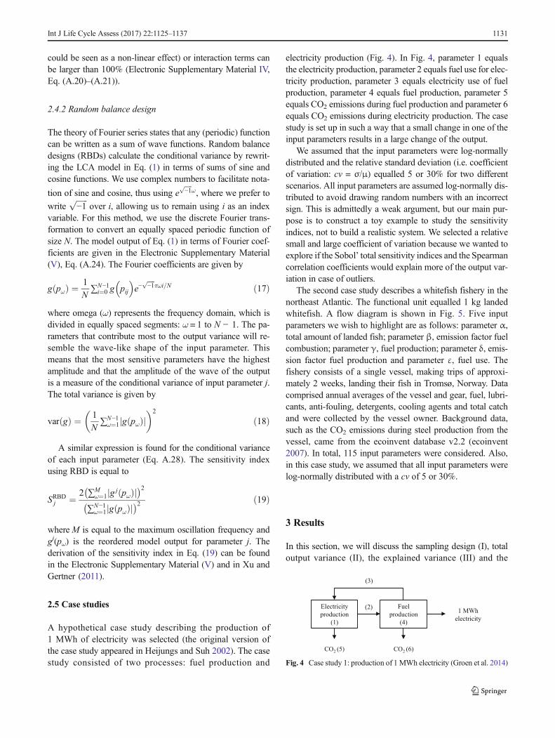
A hypothetical case study describing the production of1 MWh of electricity was selected (the original version ofthe case study appeared in Heijungs and Suh 2002). The casestudy consisted of two processes: fuel production and

electricity production (Fig. 4). In Fig. 4, parameter 1 equalsthe electricity production, parameter 2 equals fuel use for elec-tricity production, parameter 3 equals electricity use of fuelproduction, parameter 4 equals fuel production, parameter 5equals CO2 emissions during fuel production and parameter 6equals CO2 emissions during electricity production. The casestudy is set up in such a way that a small change in one of theinput parameters results in a large change of the output.

We assumed that the input parameters were log-normallydistributed and the relative standard deviation (i.e. coefficientof variation: cv = σ/μ) equalled 5 or 30% for two differentscenarios. All input parameters are assumed log-normally dis-tributed to avoid drawing random numbers with an incorrectsign. This is admittedly a weak argument, but our main pur-pose is to construct a toy example to study the sensitivityindices, not to build a realistic system. We selected a relativesmall and large coefficient of variation because we wanted toexplore if the Sobol’ total sensitivity indices and the Spearmancorrelation coefficients would explain more of the output var-iation in case of outliers.

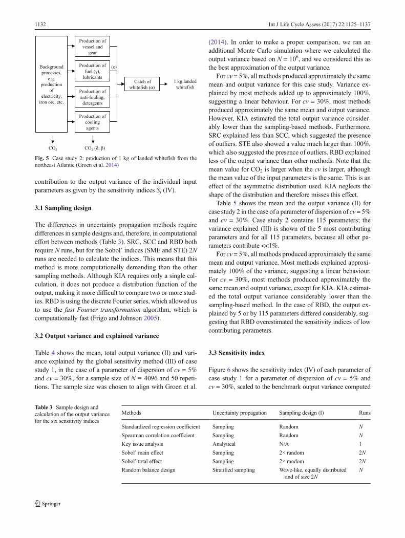
The second case study describes a whitefish fishery in thenortheast Atlantic. The functional unit equalled 1 kg landedwhitefish. A flow diagram is shown in Fig. 5. Five inputparameters we wish to highlight are as follows: parameter α,total amount of landed fish; parameter β, emission factor fuelcombustion; parameter γ, fuel production; parameter δ, emis-sion factor fuel production and parameter ε, fuel use. Thefishery consists of a single vessel, making trips of approxi-mately 2 weeks, landing their fish in Tromsø, Norway. Datacomprised annual averages of the vessel and gear, fuel, lubri-cants, anti-fouling, detergents, cooling agents and total catchand were collected by the vessel owner. Background data,such as the CO2 emissions during steel production from thevessel, came from the ecoinvent database v2.2 (ecoinvent2007). In total, 115 input parameters were considered. Also,in this case study, we assumed that all input parameters werelog-normally distributed with a cv of 5 or 30%.

3 Results

In this section, we will discuss the sampling design (I), totaloutput variance (II), the explained variance (III) and the

Electricity

production

(1)

CO2 (5) CO2 (6)

Fuel

production

(4)

1 MWh

electricity

(2)

(3)

Fig. 4 Case study 1: production of 1 MWh electricity (Groen et al. 2014)

Int J Life Cycle Assess (2017) 22:1125–1137 1131

contribution to the output variance of the individual inputparameters as given by the sensitivity indices Sj (IV).

3.1 Sampling design

The differences in uncertainty propagation methods requiredifferences in sample designs and, therefore, in computationaleffort between methods (Table 3). SRC, SCC and RBD bothrequire N runs, but for the Sobol’ indices (SME and STE) 2Nruns are needed to calculate the indices. This means that thismethod is more computationally demanding than the othersampling methods. Although KIA requires only a single cal-culation, it does not produce a distribution function of theoutput, making it more difficult to compare two or more stud-ies. RBD is using the discrete Fourier series, which allowed usto use the fast Fourier transformation algorithm, which iscomputationally fast (Frigo and Johnson 2005).

3.2 Output variance and explained variance

Table 4 shows the mean, total output variance (II) and vari-ance explained by the global sensitivity method (III) of casestudy 1, in the case of a parameter of dispersion of cv = 5%and cv = 30%, for a sample size of N = 4096 and 50 repeti-tions. The sample size was chosen to align with Groen et al.

(2014). In order to make a proper comparison, we ran anadditional Monte Carlo simulation where we calculated theoutput variance based on N = 106, and we considered this asthe best approximation of the output variance.

For cv = 5%, all methods produced approximately the samemean and output variance for this case study. Variance ex-plained by most methods added up to approximately 100%,suggesting a linear behaviour. For cv = 30%, most methodsproduced approximately the same mean and output variance.However, KIA estimated the total output variance consider-ably lower than the sampling-based methods. Furthermore,SRC explained less than SCC, which suggested the presenceof outliers. STE also showed a value much larger than 100%,which also suggested the presence of outliers. RBD explainedless of the output variance than other methods. Note that themean value for CO2 is larger when the cv is larger, althoughthe mean value of the input parameters is the same. This is aneffect of the asymmetric distribution used. KIA neglects theshape of the distribution and therefore misses this effect.

Table 5 shows the mean and the output variance (II) forcase study 2 in the case of a parameter of dispersion of cv = 5%and cv = 30%. Case study 2 contains 115 parameters; thevariance explained (III) is shown of the 5 most contributingparameters and for all 115 parameters, because all other pa-rameters contribute <<1%.

For cv = 5%, all methods produced approximately the samemean and output variance. Most methods explained approxi-mately 100% of the variance, suggesting a linear behaviour.For cv = 30%, most methods produced approximately thesame mean and output variance, except for KIA. KIA estimat-ed the total output variance considerably lower than thesampling-based method. In the case of RBD, the output ex-plained by 5 or by 115 parameters differed considerably, sug-gesting that RBD overestimated the sensitivity indices of lowcontributing parameters.

3.3 Sensitivity index

Figure 6 shows the sensitivity index (IV) of each parameter ofcase study 1 for a parameter of dispersion of cv = 5% andcv = 30%, scaled to the benchmark output variance computed

Production of

vessel and

gear

Catch of

whitefish (α)

Production of

fuel (γ),

lubricants

Production of

anti-fouling,

detergents

Background

processes,

e.g.

production

of

electricity,

iron ore, etc.

Production of

cooling

agents

1 kg landed

whitefish

CO2 CO2 (δ; β)

(ε)

Fig. 5 Case study 2: production of 1 kg of landed whitefish from thenortheast Atlantic (Groen et al. 2014)

Table 3 Sample design andcalculation of the output variancefor the six sensitivity indices

Methods Uncertainty propagation Sampling design (I) Runs

Standardized regression coefficient Sampling Random N

Spearman correlation coefficient Sampling Random N

Key issue analysis Analytical N/A 1

Sobol’ main effect Sampling 2× random 2N

Sobol’ total effect Sampling 2× random 2N

Random balance design Stratified sampling Wave-like, equally distributedand of size 2N

N

1132 Int J Life Cycle Assess (2017) 22:1125–1137

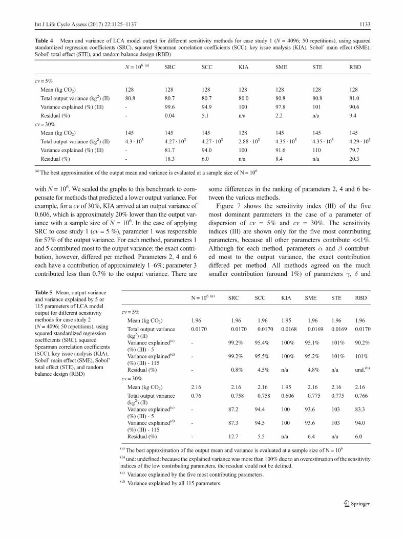
with N = 106. We scaled the graphs to this benchmark to com-pensate for methods that predicted a lower output variance. Forexample, for a cv of 30%, KIA arrived at an output variance of0.606, which is approximately 20% lower than the output var-iance with a sample size of N = 106. In the case of applyingSRC to case study 1 (cv = 5 %), parameter 1 was responsiblefor 57% of the output variance. For each method, parameters 1and 5 contributed most to the output variance; the exact contri-bution, however, differed per method. Parameters 2, 4 and 6each have a contribution of approximately 1–6%; parameter 3contributed less than 0.7% to the output variance. There are

some differences in the ranking of parameters 2, 4 and 6 be-tween the various methods.

Figure 7 shows the sensitivity index (III) of the fivemost dominant parameters in the case of a parameter ofdispersion of cv = 5% and cv = 30%. The sensitivityindices (III) are shown only for the five most contributingparameters, because all other parameters contribute <<1%.Although for each method, parameters α and β contribut-ed most to the output variance, the exact contributiondiffered per method. All methods agreed on the muchsmaller contribution (around 1%) of parameters γ, δ and

Table 4 Mean and variance of LCA model output for different sensitivity methods for case study 1 (N = 4096; 50 repetitions), using squaredstandardized regression coefficients (SRC), squared Spearman correlation coefficients (SCC), key issue analysis (KIA), Sobol’ main effect (SME),Sobol’ total effect (STE), and random balance design (RBD)

N = 106 (a) SRC SCC KIA SME STE RBD

cv = 5%

Mean (kg CO2) 128 128 128 128 128 128 128

Total output variance (kg2) (II) 80.8 80.7 80.7 80.0 80.8 80.8 81.0

Variance explained (%) (III) - 99.6 94.9 100 97.8 101 90.6

Residual (%) - 0.04 5.1 n/a 2.2 n/a 9.4

cv = 30%

Mean (kg CO2) 145 145 145 128 145 145 145

Total output variance (kg2) (II) 4.3 · 103 4.27 · 103 4.27 · 103 2.88 · 103 4.35 · 103 4.35 · 103 4.29 · 103

Variance explained (%) (III) - 81.7 94.0 100 91.6 110 79.7

Residual (%) - 18.3 6.0 n/a 8.4 n/a 20.3

(a) The best approximation of the output mean and variance is evaluated at a sample size of N = 106

Table 5 Mean, output varianceand variance explained by 5 or115 parameters of LCA modeloutput for different sensitivitymethods for case study 2(N = 4096; 50 repetitions), usingsquared standardized regressioncoefficients (SRC), squaredSpearman correlation coefficients(SCC), key issue analysis (KIA),Sobol’main effect (SME), Sobol’total effect (STE), and randombalance design (RBD)

N = 106 (a) SRC SCC KIA SME STE RBD

cv = 5%

Mean (kg CO2) 1.96 1.96 1.96 1.95 1.96 1.96 1.96

Total output variance(kg2) (II)

0.0170 0.0170 0.0170 0.0168 0.0169 0.0169 0.0170

Variance explained(c)

(%) (III) - 5- 99.2% 95.4% 100% 95.1% 101% 90.2%

Variance explained(d)

(%) (III) - 115- 99.2% 95.5% 100% 95.2% 101% 101%

Residual (%) - 0.8% 4.5% n/a 4.8% n/a und.(b)

cv = 30%

Mean (kg CO2) 2.16 2.16 2.16 1.95 2.16 2.16 2.16

Total output variance(kg2) (II)

0.76 0.758 0.758 0.606 0.775 0.775 0.766

Variance explained(c)

(%) (III) - 5- 87.2 94.4 100 93.6 103 83.3

Variance explained(d)

(%) (III) - 115- 87.3 94.5 100 93.6 103 94.0

Residual (%) - 12.7 5.5 n/a 6.4 n/a 6.0

(a) The best approximation of the output mean and variance is evaluated at a sample size of N = 106

(b) und: undefined: because the explained variance wasmore than 100% due to an overestimation of the sensitivityindices of the low contributing parameters, the residual could not be defined.(c) Variance explained by the five most contributing parameters.(d) Variance explained by all 115 parameters.

Int J Life Cycle Assess (2017) 22:1125–1137 1133

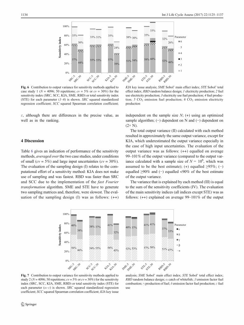
ε, although there are differences in the precise value, aswell as in the ranking.

4 Discussion

Table 6 gives an indication of performance of the sensitivitymethods, averaged over the two case studies, under conditionsof small (cv = 5%) and large input uncertainties (cv = 30%).The evaluation of the sampling design (I) relates to the com-putational effort of a sensitivity method: KIA does not makeuse of sampling and was fastest. RBD was faster than SRCand SCC due to the implementation of the fast Fouriertransformation algorithm. SME and STE have to generatetwo sampling matrices and, therefore, were slowest. The eval-uation of the sampling design (I) was as follows: (++)

independent on the sample size N; (+) using an optimizedsample algorithm; (−) dependent on N and (−) dependent on(2× N).

The total output variance (II) calculated with each methodresulted in approximately the same output variance, except forKIA, which underestimated the output variance especially inthe case of high input uncertainties. The evaluation of theoutput variance was as follows: (++) equalled on average99–101% of the output variance (compared to the output var-iance calculated with a sample size of N = 106, which wasassumed to be the best estimate); (+) equalled ≥95%; (−)equalled ≥90% and (−) equalled <90% of the best estimateof the output variance.

The variance that is explained by each method (III) is equalto the sum of the sensitivity coefficients (IV). The evaluationof the main sensitivity indices (all indices except STE) was asfollows: (++) explained on average 99–101% of the output

57%44%

55% 55% 57%

39%51% 54% 58% 60%

52%46%

35%

30%

33% 31%35%

24%

38% 30%35%

33%

32%

26%

0%

20%

40%

60%

80%

100%

Sen

siti

vty

in

dex

Parameter

6

5

4

3

2

1

Fig. 6 Contribution to output variance for sensitivity methods applied tocase study 1 (N = 4096; 50 repetitions; cv = 5% or cv = 30%) for thesensitivity index (SRC, SCC, KIA, SME, RBD) or total sensitivity index(STE) for each parameter (1–6) is shown. SRC squared standardizedregression coefficient; SCC squared Spearman correlation coefficient;

KIA key issue analysis; SME Sobol’ main effect index; STE Sobol’ totaleffect index; RBD random balance design; 1 electricity production; 2 fueluse electricity production; 3 electricity use fuel production; 4 fuel produc-tion; 5 CO2 emission fuel production; 6 CO2 emission electricityproduction

40%

38%

38% 37%41%

32%

40% 37%41% 41%

37%33%

0%

20%

40%

60%

80%

100%

Sen

siti

vty

in

dex

Parameter

ε

δ

γ

β

α56%

46%54% 55% 56%

45%52% 53% 57% 58%

51% 47%

Fig. 7 Contribution to output variance for sensitivity methods applied tostudy 2 (N = 4096; 50 repetitions; cv = 5% or cv = 30%) for the sensitivityindex (SRC, SCC, KIA, SME, RBD) or total sensitivity index (STE) foreach parameter (α–ε) is shown. SRC squared standardized regressioncoefficient; SCC squared Spearman correlation coefficient;KIA key issue

analysis; SME Sobol’ main effect index; STE Sobol’ total effect index;RBD random balance design; α catch of whitefish; β emission factor fuelcombustion; γ production of fuel; δ emission factor fuel production; ε fueluse

1134 Int J Life Cycle Assess (2017) 22:1125–1137

variance (compared the output variance calculated for eachmethod); (+) explained ≥95%; (−) explained ≥90% and (−)explained <90% of the output variance. The evaluation ofthe total sensitivity index (STE) is given by the difference withSME. If STE is equal to SME, there is no use for calculatingSTE: the bigger the difference between the two indices, themore relevant it becomes to calculate the following: (++)STE − SME ≥10%; (+) STE − SME ≥5%; (−) STE − SME<5 % and (−) STE ≈ SME.

There were some limitations to the case studies that wereused to evaluate the sensitivity methods. First, all parametersare assumed to be uncorrelated, which is a simplification be-cause of lack of data. When correlations are present, includingcorrelated inputs will increase the accuracy of the outcome ofthe global sensitivity analysis (Jacques et al. 2006; Xu andGertner 2008b). A global sensitivity index given by SRC formodels with correlated inputs can be found in Xu and Gertner(2008b), given by the Sobol’ indices in Jacques et al. (2006)and given by the RBD and its corresponding indices in Xu andGertner (2008a).

Second, the performance indicators in Table 6 are based ontwo case studies with two different sets of input parameters,which is limited. Other types of distribution functions or casestudies with more interacting input parameters, for example,were not considered. However, we assumed that not so muchthe type of distribution function will influence the set of rec-ommended methods, but that it primarily relies on the firstmoment of the input uncertainty (increasing the chance ofoutliers and the effect of interactions leading to non-linearbehaviour) (Saltelli et al. 2008).

Third, we only considered the inventory stage in this paper.Usually, an LCA includes a midpoint or even an endpointassessment. In general, the midpoint to inventory calculationstep is assumed to be linear, but the inventory to midpoint ormidpoint to endpoint relations could be non-linear; in thesecases, the Sobol’ method might be preferred because it isbetter able to include non-linear effects (Iooss and Lemaître2014; Sobol’ 2001). An illustrative example is given inCucurachi (2014), where sensitivity indices were quantified

in the case of impact assessment of noise on human health,resulting in high values for STE compared to SME, illustrat-ing the benefit of using Sobol’ indices as a measure of globalsensitivity.

Fourth, this article started from moment-based approaches,in particular the contribution to variance. An extension of ouranalysis to moment-independent approaches seems to be alogical next step.

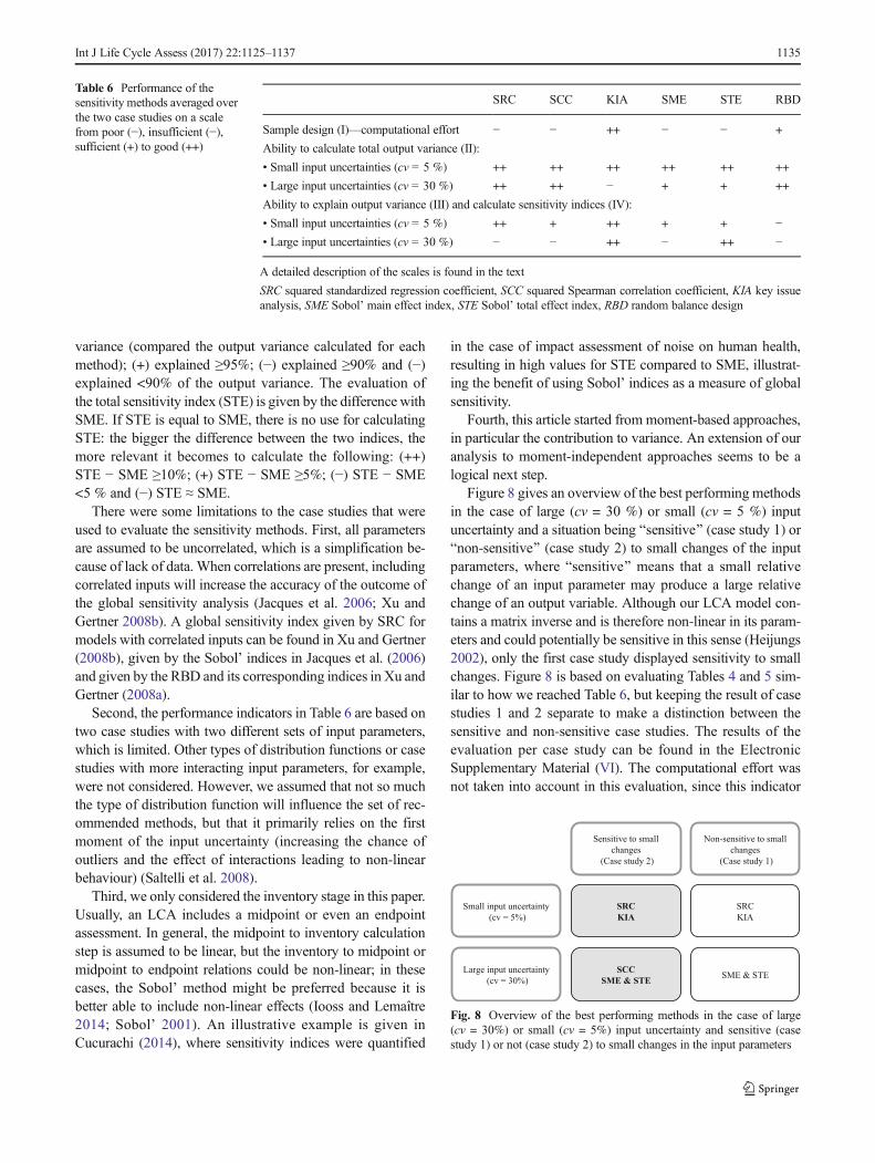
Figure 8 gives an overview of the best performing methodsin the case of large (cv = 30 %) or small (cv = 5 %) inputuncertainty and a situation being Bsensitive^ (case study 1) orBnon-sensitive^ (case study 2) to small changes of the inputparameters, where Bsensitive^ means that a small relativechange of an input parameter may produce a large relativechange of an output variable. Although our LCA model con-tains a matrix inverse and is therefore non-linear in its param-eters and could potentially be sensitive in this sense (Heijungs2002), only the first case study displayed sensitivity to smallchanges. Figure 8 is based on evaluating Tables 4 and 5 sim-ilar to how we reached Table 6, but keeping the result of casestudies 1 and 2 separate to make a distinction between thesensitive and non-sensitive case studies. The results of theevaluation per case study can be found in the ElectronicSupplementary Material (VI). The computational effort wasnot taken into account in this evaluation, since this indicator

Table 6 Performance of thesensitivity methods averaged overthe two case studies on a scalefrom poor (−), insufficient (−),sufficient (+) to good (++)

SRC SCC KIA SME STE RBD

Sample design (I)—computational effort − − ++ − − +

Ability to calculate total output variance (II):

• Small input uncertainties (cv = 5 %) ++ ++ ++ ++ ++ ++

• Large input uncertainties (cv = 30 %) ++ ++ − + + ++

Ability to explain output variance (III) and calculate sensitivity indices (IV):

• Small input uncertainties (cv = 5 %) ++ + ++ + + −• Large input uncertainties (cv = 30 %) − − ++ − ++ −

A detailed description of the scales is found in the text

SRC squared standardized regression coefficient, SCC squared Spearman correlation coefficient, KIA key issueanalysis, SME Sobol’ main effect index, STE Sobol’ total effect index, RBD random balance design

Sensitive to small

changes

(Case study 2)

Non-sensitive to small

changes

(Case study 1)

Small input uncertainty

(cv = 5%)

Large input uncertainty

(cv = 30%)

SRC

KIA

SRC

KIA

SCC

SME & STE SME & STE

Fig. 8 Overview of the best performing methods in the case of large(cv = 30%) or small (cv = 5%) input uncertainty and sensitive (casestudy 1) or not (case study 2) to small changes in the input parameters

Int J Life Cycle Assess (2017) 22:1125–1137 1135

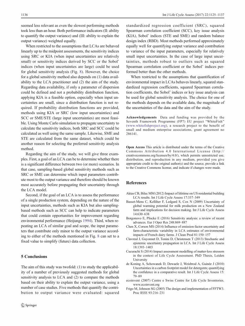
seemed less relevant as even the slowest performing methodstook less than an hour. Both performance indicators (II: abilityto quantify the output variance) and (III: ability to explain theoutput variance) weighted equally.

When restricted to the assumptions that LCAs are behavedlinearly up to the midpoint assessments, the sensitivity indicesusing SRC or KIA (when input uncertainties are relativelysmall) or sensitivity indices derived by SCC or the Sobol’indices (when input uncertainties are large) could be usedfor global sensitivity analysis (Fig. 8). However, the choicefor a global sensitivity method also depends on (1) data avail-ability to the LCA practitioner and (2) the aim of the study.Regarding data availability, if only a parameter of dispersioncould be defined and not a probability distribution function,applying KIA is a feasible option, especially when input un-certainties are small, since a distribution function is not re-quired. If probability distribution functions are provided,methods using KIA or SRC (low input uncertainties) andSCC or SME/STE (large input uncertainties) are most feasi-ble. UsingMonte Carlo simulation to propagate uncertainty tocalculate the sensitivity indices, both SRC and SCC could becalculated as well using the same sample. Likewise, SME andSTE are calculated from the same dataset, which could beanother reason for selecting the preferred sensitivity analysismethod.

Regarding the aim of the study, we will give three exam-ples. First, a goal of an LCA can be to determine whether thereis a significant difference between two (or more) scenarios. Inthat case, sampling-based global sensitivity methods such asSRC or SME can determine which input parameters contrib-ute most to the output variance and therefore should be knownmost accurately before propagating their uncertainty throughthe LCA model.

Second, if the goal of an LCA is to assess the performanceof a single production system, depending on the nature of theinput uncertainties, methods such as KIA but also sampling-based methods such as SCC can help to indicate parametersthat could contain opportunities for improvement regardingenvironmental performance (Heijungs 1994). Third, when re-peating an LCA of similar goal and scope, the input parame-ters that contribute only minor to the output variance accord-ing to either of the methods mentioned in Fig. 8 can set to afixed value to simplify (future) data collection.

5 Conclusions

The aim of this study was twofold: (1) to study the applicabil-ity of a number of previously suggested methods for globalsensitivity analysis to LCA and (2) to compare the methodsbased on their ability to explain the output variance, using anumber of case studies. Five methods that quantify the contri-bution to output variance were evaluated: squared

standardized regression coefficient (SRC), squaredSpearman correlation coefficient (SCC), key issue analysis(KIA), Sobol’ indices (STE and SME) and random balancedesign index (RBD). Most methods performed approximatelyequally well for quantifying output variance and contributionto variance of the input parameters, especially for relativelysmall input uncertainties. In the case of large input uncer-tainties, methods robust to outliers such as squaredSpearman correlation coefficient or the Sobol’ indices per-formed better than the other methods.

When restricted to the assumptions that quantification ofenvironmental impact in LCAs behaves linearly, squared stan-dardized regression coefficients, squared Spearman correla-tion coefficients, the Sobol’ indices or key issue analysis canbe used for global sensitivity analysis. The choice for one ofthe methods depends on the available data, the magnitude ofthe uncertainties of the data and the aim of the study.

Acknowledgements Data and funding was provided by theSeventh Framework Programme (FP7) EU project BWhiteFish^(www.whitefishproject.org), a research project to the benefit ofsmall and medium enterprise associations, grant agreement no286141.

Open Access This article is distributed under the terms of the CreativeCommons At t r ibut ion 4 .0 In te rna t ional License (h t tp : / /creativecommons.org/licenses/by/4.0/), which permits unrestricted use,distribution, and reproduction in any medium, provided you giveappropriate credit to the original author(s) and the source, provide a linkto the Creative Commons license, and indicate if changes were made.

References

Aktas CB, BilecMM (2012) Impact of lifetime onUS residential buildingLCA results. Int J Life Cycle Assess 17:337–349

Basset-Mens C, Kelliher F, Ledgard S, Cox N (2009) Uncertainty ofglobal warming potential for milk production on a New Zealandfarm and implications for decision making. Int J Life Cycle Assess14:630–638

Borgonovo E, Pliscke E (2016) Sensitivity analysis: a review of recentadvances. Eur J Oper Res 248:869–887

Chen X, Corson MS (2014) Influence of emission-factor uncertainty andfarm-characteristic variability in LCA estimates of environmentalimpacts of French dairy farms. J Clean Prod 81:150–157

Clavreul J, Guyonnet D, Tonini D, Christensen T (2013) Stochastic andepistemic uncertainty propagation in LCA. Int J Life Cycle Assess18:1393–1403

Cucurachi S (2014) Impact assessment modelling of matter-less stressorsin the context of Life Cycle Assessment. PhD Thesis, LeidenUniversity

de Koning A, Schowanek D, Dewaele J, Weisbrod A, Guinée J (2010)Uncertainties in a carbon footprint model for detergents; quantifyingthe confidence in a comparative result. Int J Life Cycle Assess 15:79–89

ecoinvent (2007) Centre e Swiss Centre for Life Cycle Inventories.www.ecoinvent.org

Frigo M, Johnson SG (2005) The design and implementation of FFTW3.Proc IEEE 93:216–231

1136 Int J Life Cycle Assess (2017) 22:1125–1137

Geisler G, Hellweg S, Hungerbühler K (2005) Uncertainty analysis in lifecycle assessment (LCA): case study on plant-protection productsand implications for decision making. Int J Life Cycle Assess 10:184–192

Groen EA, Heijungs R, Bokkers EAM, de Boer IJM (2014) Methods foruncertainty propagation in life cycle assessment. Environ ModelSoft 62:316–325

Hamby DM (1994) A review of techniques for parameter sensitivity anal-ysis of environmental models. Environ Monit Assess 32:135–154

Heijungs R (1994) A generic method for the identification of options forcleaner products. Ecol Econ 10:69–81

Heijungs R (1996) Identification of key issues for further investigation inimproving the reliability of life-cycle assessments. J Clean Prod 4:159–166

Heijungs R (2002) The use of matrix perturbation theory for addressingsensitivity and uncertainty issues in LCA. p. 77–80. In: Anonymous(ed) Proceedings of the fifth international conference on ecobalance.Practical tools and thoughtful principles for sustainability. Nov. 6–Nov. 8, 2002, Epochal Tsukuba, Tsukuba, Japan

Heijungs R, Lenzen M (2014) Error propagation methods for LCA—acomparison. Int J Life Cycle Assess 19:1445–1461

Heijungs R, Suh S (2002) The computational structure of life cycle as-sessment. Kluwer Academic Publishers, Dordrecht

Heijungs R, Suh S, Kleijn R (2005) Numerical approaches to life cycleinterpretation—the case of the Ecoinvent’96 database. Int J LifeCycle Assess 10:103–112

Huijbregts MJ et al (2001) Framework for modelling data uncertainty inlife cycle inventories. Int J Life Cycle Assess 6:127–132

Iooss B, Lemaître P (2014) A review on global sensitivity analysismethods. arXiv preprint arXiv:14042405

Jacques J, Lavergne C, Devictor N (2006) Sensitivity analysis in presenceof model uncertainty and correlated inputs. Reliab Eng Syst Safe 91:1126–1134

Jung J, von der Assen N, Bardow A (2014) Sensitivity coefficient-baseduncertainty analysis for multi-functionality in LCA. Int J Life CycleAssess 19:661–676

Lloyd SM, Ries R (2007) Characterizing, propagating, and analyzinguncertainty in life-cycle assessment: a survey of quantitative ap-proaches. J Ind Ecol 11:161–179

Mattila T, Leskinen P, Soimakallio S, Sironen S (2012) Uncertainty inenvironmentally conscious decisionmaking: beer or wine? Int J LifeCycle Assess 17:696–705

Mattinen MK, Heljo J, Vihola J, Kurvinen A, Lehtoranta S, Nissinen A(2014) Modeling and visualization of residential sector energy con-sumption and greenhouse gas emissions. J Clean Prod 81:70–80

McKay MD, Morrison JD, Upton SC (1999) Evaluating prediction un-certainty in simulation models. Comput Phys Commun 117:44–51

Mutel CL, de Baan L, Hellweg S (2013) Two-step sensitivity testing ofparametrized and regionalized life cycle assessments: methodologyand case study. Environ Sci Technol 47:5660–5667

Onat N, Kucukvar M, Tatari O (2014) Integrating triple bottom lineinput–output analysis into life cycle sustainability assessmentframework: the case for US buildings. Int J Life Cycle Assess19:1488–1505

Saltelli A, Sobol IM (1995) About the use of rank transformation in sensi-tivity analysis of model output. Reliab Eng Syst Saf 50:225–239

Saltelli A, Tarantola S, Chan KPS (1999) A quantitative model-independent method for global sensitivity analysis of model output.Technometrics 41:39–56

Saltelli A et al. (2008) Introduction to sensitivity aalysis. In: Global sen-sitivity analysis. The Primer. Wiley, Ltd, pp 1–51

Saltelli A, Annoni P, Azzini I, Campolongo F, Ratto M, Tarantola S(2010) Variance based sensitivity analysis of model output. Designand estimator for the total sensitivity index. Comput Phys Commun181:259–270

Sobol’ IM (2001) Global sensitivity indices for nonlinear mathematicalmodels and their Monte Carlo estimates. Math Comput Simulat 55:271–280

Sonnemann GW, Schuhmacher M, Castells F (2003) Uncertainty assess-ment by a Monte Carlo simulation in a life cycle inventory of elec-tricity produced by a waste incinerator. J Clean Prod 11:279–292

Sugiyama H, Fukushima Y, Hirao M, Hellweg S, Hungerbühler K (2005)Using standard statistics to consider uncertainty in industry-basedlife cycle inventory databases. Int J Life Cycle Assess 10:399–405

Tarantola S, Gatelli D, Mara TA (2006) Random balance designs for theestimation of first order global sensitivity indices. Reliab Eng SystSafe 91:717–727

Tarantola S, Becker W, Zeitz D (2012) A comparison of two samplingmethods for global sensitivity analysis. Comput Phys Commun 183:1061–1072

Vigne M, Martin O, Faverdin P, Peyraud J-L (2012) Comparative uncer-tainty analysis of energy coefficients in energy analysis of dairyfarms from two French territories. J Clean Prod 37:185–191

Wang E, Shen Z (2013) A hybrid data quality indicator and statisticalmethod for improving uncertainty analysis in LCA of complex sys-tem—application to the whole-building embodied energy analysis. JClean Prod 43:166–173

Wei W, Larrey-Lassalle P, Faure T, Dumoulin N, Roux P, Mathias J-D(2014) How to conduct a proper sensitivity analysis in life cycleassessment: taking into account correlations within LCI data andinteractions within the LCA calculation model. Environ SciTechnol 49:377–385

XuC, Gertner GZ (2008a) A general first-order global sensitivity analysismethod. Reliab Eng Syst Safe 93:1060–1071

Xu C, Gertner GZ (2008b) Uncertainty and sensitivity analysis formodels with correlated parameters. Reliab Eng Syst Safe 93:1563–1573

Xu C, Gertner GZ (2011) Understanding and comparisons of differentsampling approaches for the Fourier Amplitudes Sensitivity Test(FAST). Comput Stat Data An 55(1):184–198

Int J Life Cycle Assess (2017) 22:1125–1137 1137