Ocean DynamicsDOI 10.1007/s10236-014-0761-2

Methods for estimating the velocities of the Brazil Currentin the pre-salt reservoir area off southeast Brazil(23 ◦S–26 ◦S)

Tiago Carrilho Bilo · Ilson Carlos Almeida da Silveira ·Wellington Ceccopieri Belo · Belmiro Mendes de Castro ·Alberto Ricardo Piola

Received: 12 May 2014 / Accepted: 30 July 2014© Springer-Verlag Berlin Heidelberg 2014

Abstract The Brazil Current (BC) is likely the leastobserved and investigated subtropical western boundarycurrent in the world. This study proposes a simple andsystematic methodology to estimate quasi-synoptic cross-sectional speeds of the BC within the Santos Basin (23 ◦S−26 ◦S) based on the dynamic method using several combina-tions of data: Conductivity, temperature, and depth (CTD),temperature profiles, CTD and vessel-mounted AcousticDoppler Current Profiler (VMADCP), and temperatureprofiles and VMADCP. All of the geostrophic estimatesagree well with lowered Acoustic Doppler Current Profiler(LADCP) velocity observations and yield volume transportsof -5.56 ±1.31 and 2.50 ±1.01 Sv for the BC and theIntermediate Western Boundary Current (IWBC), respec-tively. The LADCP data revealed that the BC flows south-westward and is ∼100 km wide, 500 m deep, and has avolume transport of approximately -5.75 ±1.53 Sv and amaximum speed of 0.59 m s−1. Underneath the BC, theIWBC flows northeastward and has a vertical extent ofapproximately 1,300 m, a width of ∼60 km, a maximum

Responsible Editor: Pierre De Mey

T. C. Bilo (�) · I. C. A. da Silveira · B. M. de CastroInstituto Oceanografico da Universidade de Sao Paulo, Sao Paulo,Brasile-mail: tiago.bilo@usp.br

W. C. BeloCentro de Pesquisas e Desenvolvimento Leopoldo A. Miguez deMello, Petroleo Brasileiro, SA, Brasil

A. R. PiolaSeccion Dinamica Oceanica, Servicio de Hidrografia Naval(SHN), Universidad de Buenos Aires, and Instituto Franco-Argentino sobre Estudios de Clima y sus Impactos, CONICET,Buenos Aires, Argentina

velocity of ∼0.22 m s−1, and a volume transport of 4.11± 2.01 Sv. Our analysis indicates that in the absence ofthe observed velocities, the isopycnal (σ0) of 26.82 kg m−3

(∼500 dbar) is an adequate level of no motion for usein geostrophic calculations. Additionally, a simple lin-ear relationship between the temperature and the spe-cific volume anomaly can be used for a reliable firstestimate of the BC-IWBC system in temperature-onlytransects.

Keywords Brazil Current · Intermediate WesternBoundary Current · Santos Basin circulation · Geostrophicestimates

1 Introduction

The exploration and environmental control of the recentlydiscovered giant oil and gas reservoirs within the SantosBasin (23 ◦S−28 ◦S, Fig. 1), also referred as Santos Plateauarea in the oceanographic literature, have brought newdemands for operational oceanography, including improvedknowledge of the ocean circulation in Brazilian territorialwaters. These reservoirs (pre-salt reservoirs) are located inan oceanic region that is typically deeper than 1,000 mand are the result of the deposition of organic matterin microbial carbonates (or microbialites). These organicdeposits preceded the deposition of a thick-salt layer, whichmarks the Aptian during the opening of the Atlantic Oceanapproximately 120 million years ago (Meisling et al. 2001;Duarte and Viana 2007; Carminatti et al. 2008; Mohriaket al. 2010). The salt deposits drastically modified thegeomorphological profile of the Brazilian continental mar-gin and formed the Sao Paulo Plateau (3,000–3,600 m),which reduced the steepness of the continental slope and

Ocean Dynamics

replaced the continental rise within the Santos Basin(Zembruscki 1979).

The technological demands of oil and gas exploration atdepths of 1,000 to 3,500 m require adequate knowledge andmonitoring of surface waves and ocean currents. The tempo-ral and spatial variabilities of the western boundary jets alsoneed to be understood and monitored. Some of this infor-mation can be obtained from satellite observations, but theuse of such images can only provide either surface (via Syn-thetic Aperture Radar (SAR)) or depth-integrated (throughaltimetry) estimates of the circulation. In situ observationsare thus required to vertically extend and increase the levelof detail of the characterization of these currents.

In contrast to these operational requirements, the BrazilCurrent (BC) is likely the least observed and investigatedsubtropical western boundary currents in the world. Conse-quently, the BC’s mean flow and its variability are poorlyunderstood. The presence of operational, geophysical, andoceanographic vessels in the Santos Basin represent aunique opportunity to broaden the observational base ofthe BC and its associated mesoscale activity, which in turncan positively impact the exploration and production of the“Pre-Salt” reservoirs. Repeated hydro-oceanographic tran-sects will be performed by ships involved in both oil andgas exploration and environmental monitoring operations.Hence, ships equipped with different oceanographic instru-ments will allow monitoring of the BC at rates that have notbeen available previously.

This work proposes a systematic methodology to esti-mate quasi-synoptic cross-sectional speeds of the BC withinthe Santos Basin for cases in which data are acquiredby (i) a vessel-mounted Acoustic Doppler Current Profiler(VMADCP) and conductivity–temperature–depth (CTD)profiling, (ii) VMADCP and temperature profiling, (iii)only CTD profiling, and (iv) only temperature profiling.These estimates are based on the application of the dynamicmethod to calculate geostrophic velocities.

2 Western Boundary Current Patterns in the SantosBasin

Most of the available information about the surface speedsand volume transport for the BC is based on geostrophic cal-culations using the classical dynamic (geostrophic) methodreferenced to an arbitrarily chosen level of no motion. TheBC surface speeds range from -0.3 to -0.85 m s−1 (wherenegative indicates poleward currents), and the volumetransport varies from -5 to -16 Sv (1 Sv = 106 m3 s−1)(Signorini 1978; Miranda and Filho 1979; Evans et al.1983; Stramma 1989; Garfield 1990; Campos et al. 1995;Lima 1997; Silveira et al. 2001). It is difficult to com-pare the results from these studies because they employed

different zero cross-section velocity levels, ranging from500 to 1,300 m, in their geostrophic computations. In somecalculations, the BC is assumed to transport only Tropi-cal Water (TW) and South Atlantic Central Water (SACW)and, therefore, to only occupy the upper 500 m of thewater column (Stramma and England 1999). Other authorsassumed that the BC carries TW, SACW, Antarctic Interme-diate Water (AAIW), and Upper Circumpolar Deep Water(UCDW) (Memery et al. 2000) and thus assumed that theBC extends to a depth of 1,300 m.

The choice of the appropriate level of no motion to bet-ter reproduce the speeds, geometry, and transport of theBC using the dynamic method should be addressed basedon directly measured velocity profiles. Within the SantosBasin, only three studies provide such information: (Evansand Signorini 1985); (Muller et al. 1998); (Rocha et al.2014). Evans and Signorini (1985) presented a cross-isobathseries of quasi-synoptic profiles at approximately 23 ◦S,which revealed that the BC extends to depths of 400–500 mand that a counterflow is present underneath to a maxi-mum depth of 800–900 m. On the other hand, Muller et al.(1998) described the results of a currentmeter mooring linelocated at 28 ◦S that indicated that the BC extends to adepth of approximately 1,300–1,500 m. Rocha et al. (2014)presented an analysis of a 12-month time series from a cur-rentmeter mooring deployed at 25 ◦S that indicated that thevelocity pattern at this latitude resembles that reported byEvans and Signorini (1985) .

The answer to this apparent dichotomy in the verticalextent of the BC was provided by Boebel et al. (1999), whoperformed an analysis of trajectories of Lagrangian floatsand explained that both the AAIW and UCDW reach theSouth American continental margin from the east as partof the intermediate-upper deep parts of the South AtlanticSubtropical Gyre. The AAIW/UCDW flow splits into twobranches as it hits the southern portion of the Santos Basin.This flow split was named by the authors as the SantosBifurcation; one branch turns poleward, and the other goesthrough a cyclonic loop before turning toward the equator(Fig. 1). The axis of the Santos Bifurcation is located atapproximately 27 ◦S (Legeais et al. 2013). The northward-flowing branch of the AAIW/UCDW organizes itself as anarrow elliptically-shaped undercurrent that is commonlyreferred to as the Intermediate Western Boundary Current(IWBC). This undercurrent flowing opposite to the BCimposes a quiescent level at approximately 500 dbar.

While the appropriate choice of the level of no motion isapparently immediate upon examining the literature, thereis no quantitative assessment of whether the geostrophicvelocity estimates referenced to 500 dbar are good proxiesfor the observed meandering BC flow and therefore if thoseestimates can reproduce the appropriate partition betweenthe barotropic and baroclinic components of the BC. We

Ocean Dynamics

Fig. 1 Schematics of the Brazil Current (BC), the Intermediate West-ern Boundary Current (IWBC) and the Santos Bifurcation flow patternbased on Boebel et al. (1999) and Legeais et al. (2013) (upper panel).The dashed box indicates the area shown in detail in the lower panel.The circles represent the locations of the CTD/LADCP stations of theCERES Experiment cruise. The location of the COROAS mooring isrepresented by the star, and the triangles indicate the locations of theCTD stations of the COROAS transect

also test how the different geostrophic velocity estimatescompare to the currents that have been observed from top–bottom profiling by Lowered-ADCP (LADCP). We maketheses comparisons by focusing on the BC at 26 ◦S.

3 Data and methods

3.1 The data set

Two data sets are used in this work. The first is a his-torical data set from the COROAS experiment, which wasthe Brazilian component of the World Ocean CirculationExperiment (WOCE) (Campos et al. 1996). This data set

consists of a four-level currentmeter mooring and a repeatedquasi-synoptic hydrographic transect off the city of Santos(Fig. 1). The mooring was deployed over the 1,000 m iso-bath (25.55 ◦S, 44.93 ◦W) approximately 17 km from thetransect, and the currentmeters were placed at depths of 29,91, 293, and 698 m. The time series extend from 21 Decem-ber 1992 to 20 March 1994. The hydrographic transect wasrepeated during the HM 1 (January 20, 1993–February 03,1993), HM 2 (July 17, 1993–July 29, 1993) and HM 3(January 20, 1994–January 19, 1994) cruises.

The second data set is part of the CERES experiment,which consisted of five quasi-synoptic hydrographic surveysto investigate the BC and its recirculation cells within thepre-salt reservoir area. Here, we analyze one transect fromthe fourth cruise (June 2010), which consisted of simultane-ous top–bottom CTD and LADCP profiling. The locationsof the CERES experiment stations are shown in Fig. 1.Underway, continuous 75 kHz VMADCP observations fromthe surface to approximately 300 m was also obtained.

The data sets are used in this study as follows. InSection 4, the COROAS currentmeter mooring and hydro-graphic transects are used to evaluate how the zero cross-section velocity level changes with time and how applicablethe 500 dbar average level of no motion is to the temporally-evolving BC. In Section 5, we compare the observed top–bottom velocity patterns with the geostrophic estimatesconsidering the different data sources that are available, aswas discussed in Section 1.

3.2 Methods

3.2.1 Processing of the COROAS mooring data

Each currentmeter time series was low-pass filtered using aLanczos squared filter with a 40h cut-off (e.g., Emery andThomson 2001 to primarily retain the subinertial oscilla-tions. The inertial period at the mooring location is 27.74 h.The daily averaged velocity vectors are presented in aCartesian coordinate system that is rotated 45◦ clockwiseso the x-axis and y-axis are the along and normal direc-tions to the COROAS hydrographic transect, respectively(Fig. 2).

We then follow Silveira et al. (2008) and Rocha et al.(2014) in interpolating the four instrument levels to obtaina smoothed profile of the horizontal velocity and to inferthe velocity inversion depth (i.e., the zero cross-sectionvelocity level). The method consists of projecting thediscrete velocity values at the currentmeter depths ontothe quasi-geostrophic dynamic modes of the vertical struc-ture (the barotropic and the first three baroclinc modes).We computed the dynamic modes using a mean strat-ification frequency profile N2(z) calculated from theWorld Ocean Atlas 2013 (WOA13) climatology. The 117

Ocean Dynamics

Dec/92 Mar/93 Jun/93 Sep/93 Dec/93 Feb/94

698

293

91

29

1 m s−1

Time (month/year)

Depth

(m

)

HM 1 HM 2 HM 3

Fig. 2 Low-passed filtered and rotated current time series for the 29,91, 293, and 698 m levels of the COROAS mooring (25.55 ◦S, 44.93◦W). The scaling vector of 1.0 m s−1 is oriented along the COROAStransect shown in Fig. 1. The shaded bars denote the periods duringwhich the COROAS hydrographic surveys were conducted

climatological temperature (Locarnini et al. 2013) and salin-ity (Zweng et al. 2013) profiles over the continental slope(23 ◦S–26 ◦S) were averaged to generate the potentialdensity σ0(z) and N2(z) profiles (Fig. 3, left panel).

3.2.2 The dynamic method

The geostrophic estimates carried out in this work are basedon the classic dynamic method expression given by Eq. 1.

v(p) = vr + 1

f0

∫ pr

p

∂δ

∂xdp′, (1)

where v(p) is the cross-sectional velocity at the pressurelevel p, vr is the known velocity at the reference isobariclevel pr [vr = v(pr)], δ is the specific volume anomaly, f0

is the Coriolis parameter, and x is the along-section coordi-nate. The variations in how to apply Eq. 1 are based on howto identify or define vr and/or to obtain δ within the SantosBasin.

3.2.3 LADCP and VMADCP data processing

During the CERES experiment, velocity profiles wereobtained using a downward-looking 300 kHz LADCPWorkhorse Sentinel from RD Instruments. The averagevelocity profile at each station was calculated following

Cross-section velocity (m s )

V(507 dbar) = 0

Total

Barotropic

N (10 rad s )

Pressure

(dbar)

24.0 25.0 26.0 27.0 28.0

(kg m )

(507 dbar) = 26.82

TW-SACW

SACW-AAIW

Fig. 3 Climatological N2(z) and σ0 profiles (left panel), and the verti-cal profile of the mean cross-section velocity (right panel) at 25.55 ◦S,44.93 ◦W. The shaded green regions correspond to the TW-SACWand SACW-AAIW interfaces from Memery et al. (2000). The blackdots mark the four discrete mean currentmeter values at the current-meter depths. The red line represents the mean barotropic velocitycomponent, and the magenta line indicates the depth of the mean zerocross-section velocity level

the procedures described by Fischer and Visbeck (1993)and Visbeck (2002). The ocean velocities in the first400 m, which were measured simultaneously by a 75 KHzVMADCP Ocean Surveyor (also from RD Instruments),were included in the LADCP data processing to additionallyconstrain the solution of the inverse problem. This method-ology reduces errors because the constraints from bottomtracking and the upper ocean velocities force the averagevelocity profile to agree with these more accurate data (e.g.,Visbeck, 2002, Schott et al. 2005). The VMADCP dataprocessing was conducted using the processing softwareCommon Ocean Data Access System (CODAS) from theCurrents Group of the University of Hawaii.

4 COROAS mooring and hydrographic transects

4.1 COROAS mooring

The filtered and rotated velocity time series of the fourmeasured levels of the COROAS Mooring are presentedin Fig. 2. The upper three levels are clearly within theBC domain due to the generally southwestward flow direc-tion. The speed near the surface reaches 1.10 m s−1, butits mean value is 0.55 m s−1 with a standard deviation of0.23 m s−1. The velocity decays monotonically with depthwithin the BC. Significant and vertically-coherent variabil-ity is observed in the three upper levels, but only four events

Ocean Dynamics

of flow reversal are observed during the 15 months of theseries. This differs from the BC activity reported by Silveiraet al. (2008) and Rocha et al. (2014) near Cape Seo Tome(22 ◦S) and Cape Frio (23 ◦S), where longer and more fre-quent flow reversals were reported. The currentmeter at thedeepest level is within the IWBC and shows a mean speedof 0.12 m s−1 to the northeast and a standard deviation of0.09 m s−1. The maximum observed IWBC speed is 0.45 ms−1.

The modal projection procedure described inSection 3.2.1 was performed at each time step of the timeseries to obtain the velocity profile time series. Becausewe want to evaluate both the mean velocity profile and thetime dependency of the zero cross-section velocity level,we computed the average velocity profile over the mooringperiod (Fig. 3, right panel) and identified the level of nomotion at each time step. This mean velocity profile hasmaximum southwestward velocities of -0.55 m s−1 andnortheastward velocities of 0.12 m s−1, as was describedabove. Figure 4 illustrates the time series of the level of zerocross-section velocity at the profiles that contain veloc-ity inversions. The level of no motion oscillates around500 dbar with a mean value of 507 dbar and a standarddeviation of 131 dbar.

Because we also wish to relate the zero cross-sectionvelocity level to the interfaces between the water masses inthe Santos Basin, we used the isopycnal interfaces estimatedby Memery et al. (2000). These density values were con-verted to σ0(z), and we searched for the pressure levels atwhich they occur in the climatological σ0(z) profile (Fig. 3,

Dec/92 Mar/93 Jun/93 Sep/93 Dec/93 Feb/94

0

100

200

300

400

500

600

700

800

900

1000

1100

HM 1 HM 2 HM 3

Time (month/year)

Lev

el o

f n

o m

oti

on

(d

bar

)

Fig. 4 Time series of the zero cross-section velocity level esti-mated from the COROAS currentmeter data. The horizontal solidline shows the mean value of the time series (507 dbar). The shadedbars denote the periods during which the COROAS hydrographic sur-veys were conducted. The mooring was deployed over the 1,000 m(∼1,009.20 dbar) isobath

left panel). The depth ranges of the water mass interfacesare presented in Table 1.

Figure 3 (right panel) depicts the average BC-IWBC sys-tem that is described above. As pointed out by Rocha et al.(2014), the barotropic velocity component is approximately-0.1 m s−1 over the 1,000 m isobath. The panels fromFig. 3 illustrate the relationship between the water massand velocity pattern that is described in the literature. Thelevel of no motion is similar to the SACW-AAIW interfacefrom Memery et al. (2000) (within ∼50 dbar), which indi-cates that this interface level represents the transition depthbetween the BC and the IWBC within the Santos Basin.

4.2 Hydrographic transects

To evaluate whether the SACW-AAIW interface is a suit-able level of no motion, we carried out geostrophic estimates(Eq. 1) from the COROAS repeated quasi-synoptic hydro-graphic transect. The geostrophic velocities are computedrelative to the isopycnal level of no motion (e.g., Stramma etal. 1995). The climatological isopycnal level (26.82 kg m−3)at the corresponding no motion pressure level (507 dbar)observed in the mooring is used as reference (see Fig. 3). Allof the hydrographic transects also showed the 26.82 kg m−3

isopycnal at a mean level of approximately 500 dbar. Thismethod represents a rough and simple assessment of theBC system that does not require shoreward extrapolationsof the mass field, although the transports and a comparisonbetween the geostrophic estimates and the mooring data canindicate whether 500 dbar is an appropriate reference level.

The BC and IWBC transports were computed using thewell-defined areas of the velocity cores presented in Figs. 5,6, and 7. Following Rocha et al. (2014), the RMS dif-ferences between the geostrophic profiles closest to themooring location at each transect and the cruise-periodaverage velocity profile from the mooring were also com-puted. The HM 1 transect (Fig. 5) shows that the BC flowssouthwestward with a maximum velocity of approximately-0.40 m s−1 and a transport of -3.59 Sv. The IWBC isdepicted as a northeastward flow with a maximum veloc-ity of ∼0.23 m s−1 and a transport of 2.35 Sv, and its coreis located directly beneath the BC’s core. The geostrophicvelocity profile at the mooring location accurately repre-sents the velocity structure from the mooring observations

Table 1 Pressure levels of the water mass interfaces from Memeryet al. (2000) on the continental slope of the study region (23 ◦S–26 ◦S)

TW-SACW SACW-AAIW

σ0 (kg m−3) 25.60 ± 0.03 26.90 ± 0.01

Pressure range (dbar) 89 ± 6 563 ± 10

The pressure ranges correspond to the 95 % confidence intervals

Ocean Dynamics

Fig. 5 a Geostrophic velocity for the HM 1 transect referenced atthe 26.82 kg m−3 isopycnal level (magenta line) and b comparison ofthe geostrophic velocity profile and mooring velocity (time-averagedover the period of the cruise). Black triangles represent the hydrog-

raphic stations, and the white triangles represent the positions of thegeostrophic velocity profiles. The gray line and markers represent thepositions (along-section) of the mooring and the instrument pressurelevels, respectively

with a RMS of 0.09 m s−1. The main difference is thesharper decay of the geostrophic velocity with depth in theBC domain.

The HM 2 transect (Fig. 6) shows that the BC has a max-imum surface velocity of -0.8 m s−1 and a volume transportof -6.71 Sv. The IWBC has a maximum velocity approx-imately 0.13 m s−1 and a transport of 2.96 Sv. Note thatthe BC and IWBC cores are not aligned along the x-axis asin the HM 1 transect. Both sections show the IWBC coreat ∼900 dbar, but the IWBC is displaced offshore from theBC core in the HM 2 transect. This pattern is also sug-gested by the currentmeter data (Fig. 6, right panel). Thegeostrophic velocity profile at the mooring location rep-resents the mooring profile fairly well; the RMS betweenthem is 0.08 m s−1.

Finally, the HM 3 transect is presented in Fig. 7.Unlike the situations observed in Figs. 5 and 6, the HM3cruise shows a very weak cross-section BC-IWBC system.The BC core has maximum velocities of approximately-0.22 m s−1 at subsurface levels (∼50 dbar) and a vol-ume transport of -1.50 Sv. At intermediate levels (800-1,000 dbar), the IWBC core has maximum velocities of∼0.12 m s−1 and a transport of 0.24 Sv. Offshore from

the IWBC, there is a southwestward flow with veloci-ties of less than 0.06 m s−1. Note that in the right panelof Fig. 7, the geostrophic velocity profile at the moor-ing site has a similar flow pattern to the mooring profile,yielding a RMS of 0.09 m s−1. The low cross-sectionalBC velocities may be related to its meandering activity(e.g., Rocha et al. 2014).

The cruise periods analyzed here illustrate three distinctsituations of the BC in terms of the speed (corroborated bythe mooring observations) and, consequently, volume trans-ports. Campos et al. (1995) and Rocha et al. (2014) foundthat the BC flows southwestward transporting approxi-mately -5.7 Sv in the same region. We found a comparablevalue only in the HM 2 transect (-6.71 Sv); however, thedeeper reference levels (750 and 900 dbar) used by Camposet al. (1995) overestimated the BC’s vertical extent, and noIWBC was observed.

In the IWBC domain, the HM 1 and HM 2 transectsshow intermediate flows that are consistent with thosefound in the literature; the core is close to the conti-nental slope, the maximum velocities range from 0.13 to0.23 m s−1, and the current reaches depths greater than1,500 dbar (e.g., Evans and Signorini 1985; Silveira and

Fig. 6 Similar to Fig. 5 but forthe HM 2 transect

Ocean Dynamics

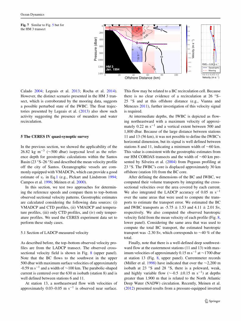
Fig. 7 Similar to Fig. 5 but forthe HM 3 transect

Calado 2004; Legeais et al. 2013; Rocha et al. 2014).However, the distinct scenario presented in the HM 3 tran-sect, which is corroborated by the mooring data, suggestsa possible perturbed state of the IWBC. The float trajec-tories presented by Legeais et al. (2013) also show suchactivity suggesting the presence of meanders and waterrecirculation.

5 The CERES IV quasi-synoptic survey

In the previous section, we showed the applicability of the26.82 kg m−3 (∼500 dbar) isopycnal level as the refer-ence depth for geostrophic calculations within the SantosBasin (23 ◦S–26 ◦S) and described the mean velocity profileoff the city of Santos. Oceanographic vessels are com-monly equipped with VMADCPs, which can provide a goodestimate of vr in Eq.1 (e.g., Pickart and Lindstrom 1994;Campos et al. 1996; Meinen et al. 2000).

In this section, we test two approaches for determin-ing the reference speeds and compare them to top–bottomobserved sectional velocity patterns. Geostrophic estimatesare calculated considering the following data sources: (i)VMADCP and CTD profiles, (ii) VMADCP and tempera-ture profiles, (iii) only CTD profiles, and (iv) only temper-ature profiles. We used the CERES experiment data set toperform these study cases.

5.1 Section of LADCP-measured velocity

As described before, the top–bottom observed velocity pro-files are from the LADCP transect. The observed cross-sectional velocity field is shown in Fig. 8 (upper panel).Note that the BC flows to the southwest in the upper500 dbar with maximum surface velocities of approximately-0.59 m s−1 and a width of ∼100 km. The parabolic-shapedcurrent is centered over the 630 m isobath (station 8) and iswell defined between stations 6 and 11.

At station 13, a northeastward flow with velocities ofapproximately 0.03–0.05 m s−1 is observed near surface.

This flow may be related to a BC recirculation cell. Becausethere is no clear evidence of a recirculation at 26 ◦S–25 ◦S and at this offshore distance (e.g., Vianna andMenezes 2011), further investigation of this velocity signalis required.

At intermediate depths, the IWBC is depicted as flow-ing northeastward with a maximum velocity of approxi-mately 0.22 m s−1 and a vertical extent between 500 and1,800 dbar. Because of the large distance between stations11 and 13 (56 km), it was not possible to define the IWBC’shorizontal dimension, but its signal is well defined betweenstations 8 and 11, indicating a minimum width of ∼60 km.This value is consistent with the geostrophic estimates fromour HM COROAS transects and the width of ∼60 km pre-sented by Silveira et al. (2004) from Pegasus profiling at23 ◦S. The IWBC’s core is displaced approximately 30 kmoffshore (station 10) from the BC core.

After defining the dimensions of the BC and IWBC, wecomputed their volume transports by integrating the cross-sectional velocities over the area covered by each current.We also integrated the LADCP accuracy of 0.05 m s−1

over the same areas that were used to compute the trans-ports to estimate the transport error. We estimated the BCand IWBC transports as -5.75 ± 1.53 and 4.11 ± 2.01 Sv,respectively. We also computed the observed barotropicvelocity field from the mean velocity of each profile (Fig. 8,lower panel). Considering the same area that was used tocompute the total BC transport, the estimated barotropictransport was -2.30 Sv, which corresponds to ∼40 % of thetotal.

Finally, note that there is a well-defined deep southwest-ward flow at the easternmost stations (11 and 13) with max-imum velocities of approximately 0.15 m s−1 at ∼1700 dbarat station 13 (Fig. 8, upper panel). Currentmeter records(Muller et al. 1998) have indicated that over the ∼2,200 misobath at 23 ◦S and 28 ◦S, there is a poleward, weak,and highly variable flow (∼-0.5 ±0.15 m s−1) at depthsgreater than 1,900 m that is related to the North AtlanticDeep Water (NADW) circulation. Recently, Meinen et al.(2012) presented results from a pressure-equipped inverted

Ocean Dynamics

Fig. 8 Cross-sectional velocitytransect measured by LADCP(upper panel) and itscorresponding barotropiccomponent (lower panel).Negative velocities aresouthwestward, and thetriangles indicate the locationsof the stations

echo sounder array at 34.5 ◦S that revealed a weak butwell-organized poleward NADW flow associated with theDeep Western Boundary Current (DWBC). Thus, to verifyif we observed the DWBC signal at stations 11 and 13, weperformed a simple water mass analysis.

The TS diagram and the potential temperature and salin-ity transects overlaid on Memery et al. (2000) water massinterfaces (Fig. 9) show the presence of five typical mid-latitude water masses in the South Atlantic: TW, SACW,AAIW, UCDW, and NADW. Combining the sectional distri-bution of the water masses together with the velocity sectionclearly illustrates the known western boundary circulationwithin the Santos Basin. The TW and SACW follow the pathof the BC in the upper 500 dbar, and the AAIW and UCDWare advected by the IWBC at intermediate depths.

Using the water mass interfaces proposed by Memeryet al. (2000), the NADW was found to be deeper than1,500 dbar at stations 10, 11, and 13. This indicates thatthe southwestward flow observed in the LADCP data maybe part of the DWBC. In addition, we tested the NADWdefinition described by Preu et al. (2013) for the ArgentineBasin: neutral density between 27.90 and 28.10 with a salin-ity greater than 34.8 PSU. Though this criterion places the

UCDW-NADW interface at a slightly deeper level, is alsoindicates that NADW occupies the deepest portions of theeasternmost stations (10–13, Fig. 9b).

5.2 Geostrophic velocity estimates

Based on the observations described in the previous sec-tions, we propose a systematic methodology for estimatinggeostrophic velocities based on the type of data available.All of the estimates are simple versions of well-establishedmethodologies that can be easily used to monitor theBrazil Current (23 ◦S–26 ◦S). In Sections 5.2.1 to 5.2.4,we describe the study cases and present the results. InSection 5.2.5, we discuss the performance of each case andits uncertainties.

5.2.1 VMADCP and CTD profiling

When both VMADCP and CTD profiles are available,geostrophic velocities can be estimated by combining therelative geostrophic velocity with the VMADCP absolutevelocity (vr = VV MADCP in Eq. 1). The method con-sists of calculating the absolute (barotropic + baroclinic)

Ocean Dynamics

Fig. 9 TS Diagram a and potential temperature and salinity sectionsb for the CERES transect. The color scheme indicates the observedwater masses following the σ0 interfaces described by (Memery et al.2000). The shaded area in b represents presence of the NADW basedon the criterion of (Preu et al. 2013)

geostrophic velocity profile averaged between two CTDstations. This kind of approach has the advantage of notrequiring an arbitrarily chosen level of no motion; therefore,the barotropic component is estimated from direct veloc-ity observations. This methodology is based on Pickart andLindstrom (1994) and Cokelet et al. (1996), who definedhow VV MADCP should be applied as vr . Ideally, we mustuse the geostrophic component of the VV MADCP as ref-erence. However, VMADCP measures the total velocityin the upper ocean. For a potential vr , we considered theVV MADCP that obeys two basic criteria: it must be locatedat a pressure level off the Ekman layer, and it has to be inthe equipment’s depth range of operation.

Fig. 10 Absolute geostrophic velocity profiles (solid blue lines) andaverage VMADCP cross-sectional velocity profiles (dashed red lines).The black dots indicate the reference depths used

To define the first criterion, we computed the meanEkman layer depth (DE) within the Santos Basin for theCERES cruise. The estimates were made using sea surfacewind from the National Center for Environmental Prediction(NCEP) Reanalysis and AVISO daily wind speed data. Weestimated DE using Eq. 2 Cushman-Roisin B and BeckersJM (1994).

DE = γ

f0

√|τ |ρ0

, (2)

where γ =0.4 is the Von Karman’s constant, |τ | is the mag-nitude of the wind stress, and ρ0 is the mean density ofthe mixed layer observed in the CERES hydrographic tran-sect. The results show that DE is ∼45.6 m (45.9 dbar) and∼35.3 m (35.5 dbar) when calculated from the NCEP andAVISO data, respectively.

From the Ekman theory and assuming a constant eddyviscosity of 0.05 m2 s−1, the wind-driven current speed at

Table 2 Reference levels employed in the VMADCP-referenceddynamic method

Stations Offshore Bathmetry (m) Reference

distance (km) Pressure (dbar)

4-5 8 196 128

5-6 23 325 133

6-7 38 587 172

7-8 52 937 210

8-9 66 1,418 167

9-10 82 1,876 298

10-11 102 2,299 212

11-13 143 2,431 160

Ocean Dynamics

Fig. 11 VMADCP-referencedabsolute geostrophic velocitytransect. Negative velocities aresouthwestward, black trianglesindicate the locations of thestations, and white trianglesrepresent the locations of thegeostrophic profiles

100 dbar corresponds to ∼7 % of the surface speed (VE).The value of VE obtained using the NCEP (AVISO) windstress is ∼0.024 (0.023) m s−1. Therefore, the BC veloc-ities at 100 dbar are two orders of magnitude higher thanthe wind-driven current speed at this isobaric level. Becausethe velocity was measured by a 75 kHz VMADCP, we ref-erenced our calculations between the 100 and 300 dbarpressure levels. This procedure guarantees that both criteriaare satisfied.

We spatially averaged the VMADCP cross-sectionalvelocity profiles between the CTD stations to obtain themean VMADCP profiles at the same locations as thegeostrophic profiles. The reference level was then chosenby matching the VMADCP and relative geostrophic profilesin a least-squares sense. Figure 10 illustrates the referenceprofiles and the resulting absolute geostrophic velocities atselected station pairs. All of the reference levels employedare presented in Table 2.

The ADCP-referenced geostrophic velocity field isshown in Fig. 11. The BC is depicted as a southwestwardflow with maximum surface velocities of approximately -0.60 m s−1 (stations 7 and 8) and a volume transport of

Fig. 12 Linear fit of the climatological temperature-specific volumeanomaly (δ) curve in the Santos Basin

-6.77 Sv. At stations 8 and 9, the BC appears to extenddown to 600 dbar. At intermediate levels, the IWBC signalis restricted to stations 9–11 and extends from 500 dbar to∼1,700 dbar, yielding a volume transport of 1.02 Sv. TheIWBC core is centered at stations 9 and 10 with maximumvelocities of approximately 0.24 m s−1 at 1,000 dbar.

5.2.2 VMADCP and temperature (T) profiling

As pointed out in Section 1, vessels equipped with differentoceanographic sensors will be operating within the pre-saltreservoir area. These vessels, which cannot stop operatingto deploy LADCP or CTD, can also be used to estimategeostrophic velocities.

Based on the relationship between the climatologicaltemperature (T) and the specific volume anomaly (δ), weestablished a form to derive the mass field from only verti-cal temperature profiles. This kind of approach is useful fordata acquired by supply vessels equipped with instrumentssuch as Expendable Bathythermographs (XBTs).

We calculated the mean δ profile from the WOA13 tem-perature (Locarnini et al. 2013) and salinity (Zweng et al.2013) data within the study region. Based on this averagedcurve, we modeled the relationship between T and its asso-ciated δ using a linear fit. The model is presented in Fig. 12and Eq. 3.

δ(T) = [0.0988T + 0.3635].10−6. (3)

To test Eq. 3, we computed δ from the CERES CTDtemperature profiles and the VMADCP-referenced abso-lute geostrophic velocity. The XBT-like derived geostrophicvelocity transect is shown in Fig. 13. The velocity patternis similar to that obtained in Section 5.2.1, which suggeststhat the linear fit is a satisfactory model. Note that the BChas maximum velocities of -0.57 m s−1 (stations 7 and 8)and a volume transport of -6.55 Sv. At depths greater than500 dbar, the IWBC flows northeastward with a maximum

Ocean Dynamics

Fig. 13 Similar to Fig. 11 butfor the geostrophic velocityderived from only temperatureprofiles

Fig. 14 Isopycnal(26.82 kg m−1, magenta line)referenced absolute geostrophicvelocity transect. Negativevelocities are southwestward,black triangles indicate thelocations of the stations, andwhite triangles represent thelocations of the geostrophicprofiles

Fig. 15 Similar to Fig. 14 butfor the geostrophic velocityderived from only temperatureprofiles

Ocean Dynamics

velocity of ∼0.26 m s−1 (stations 9 and 10) and a volumetransport of 3.13 Sv. We should emphasize that this calcu-lation differs from that presented in Section 5.2.1 solely bythe computation of δ.

5.2.3 CTD profiling

If VMADCP data are not available, absolute geostrophicvelocities can be estimated using the isopycnal depth of26.82 kg m−3 as the zero cross-section velocity level (seeSection 4). As expected, the mean pressure at the CEREStransect that corresponds to the isopycnal 26.82 kg m−3 isapproximately 500 dbar (Fig. 9).

Figure 14 presents the resulting geostrophic field. Onceagain, the BC is depicted as having a width of approxi-mately 100 km (stations 5 and 6 to 10 and 11) and a verticalextent of ∼500 dbar. Its maximum surface velocities reach-0.38 m s−1 (stations 7 and 8), and the volume transport is -4.07 Sv. The IWBC signal is clear from stations 8-9 to 10-11and has maximum intensities of 0.26 m s−1 (stations 9-10)at ∼1,000 dbar. The volume transport at intermediate depthsis 2.72 Sv.

5.2.4 Temperature (T) profiling

Assuming that only temperature profiles are available, abso-lute geostrophic velocities can be estimated by applyingEq. 3 and the isopycnal level of 26.82 kg m−3 as reference(∼500 dbar). Before performing the referencing, the spe-cific volume anomaly (δ) field obtained from Eq. 3 is addedto the standard specific volume and used to obtain the poten-tial density (σ0) field. The results are shown in Fig. 15. Notethat both the BC and IWBC have shapes and dimensions thatare comparable to those obtained using the other methods.The BC’s core is centered at stations 8-9 with maximumsurface intensities of approximately -0.41 m s−1, and itsvolume transport is -4.86 Sv. The IWBC’s core is locatedat ∼1,000 dbar (stations 9-10) and has a maximum veloc-ity of 0.28 m s−1 and a volume transport of approximately3.13 Sv.

5.2.5 Methodology performance and uncertainties

The geostrophic velocity fields obtained in the previoussections (Figs. 11, 13, 14, and 15) are in good qualitativeagreement with the directly observed velocity field fromLADCP measurements (Fig. 8). To quantify how similarthe geostrophic estimates are to the LADCP measurements,we linearly interpolated the LADCP observations to thegeostrophic grid and compared the velocity profiles.

Figure 16 shows the absolute difference fields betweenthe geostrophic estimates and the interpolated LADCP pro-files. Note that the VMADCP-referenced method (panels a

and b) yielded better estimates in the BC current domain(pressures < 500 dbar; stations 5-6 to 10-11) comparedto the level of no motion assumption (panels c and d).At the BC’s core (stations 7 and 8), the isopycnal method(panel c) underestimated the barotropic component by 0.08–0.24 m s−1, which is clearly due to the fact that the BCoccupies the entire water column at stations 7 and 8, and theno motion level is not observed (Fig. 8).

At pressures greater than 500 dbar, the level of no motionassumption performed as well as the VMADCP-referencedmethods. This further confirms that the isopycnal level of26.82 kg m−3 (∼500 dbar) can be used as reference. Thesimilar difference distributions (Fig. 16, left and right pan-els) also indicate that the applied linear relationship betweenδ and T (Eq. 3) is a reasonable first-order approximation.

We plotted the geostrophic profiles closest to the BC andIWBC cores in Fig. 17 with the corresponding interpolatedLADCP profiles. As we observed before, the barotropiccomponent from the VMADCP is better represented (seesmaller RMS differences in panels a and b) than in theisopycnal methods (panels c and d). Another importantaspect is the vertical shear of the LADCP observed veloci-ties; the LADCP shear is similar to the geostrophic shear, inparticular outside the ageostrophic area at pressures greaterthan 100 dbar, which reinforces the applicability of themethods used in this study. As expected, if the geostrophiccalculations are properly applied, the BC-IWBC system canbe represented accurately.

Finally, we recomputed the LADCP-derived volumetransports of the BC and IWBC using the average velocityprofiles between two consecutive station locations (linearlyinterpolated profiles). This simple difference in estimatingthe transports aimed a more adequate and precise directcomparison between the transports inferred from geostro-phy and those calculated from directly observed veloci-ties. The new transport values for the station-pair aver-aged LADCP of the BC and the IWBC are -5.12±0.88and 2.01±0.61 Sv, respectively. Table 3 summarizes thegeostrophic and LADCP transport estimates. Our fourgeostrophic estimates yield mean volume transports of -5.56±1.31 and 2.50 ±1.01 Sv for the BC and IWBC, respec-tively. The ranges of the geostrophic volume transportsrepresent the standard deviations of the four values.

Despite the good agreement between the geostrophicestimates and the direct observations, the errors and uncer-tainties involved in such geostrophic estimates must beconsidered. Johns et al. (1989) stated that the overall error inthe geostrophic velocity (dvg) can be estimated by assumingthree primary sources of uncorrelated errors (Eq. 4).

dvg =√

(d�D

f L)2 + (

dL

Lvg)2 + (dvr)2. (4)

Ocean Dynamics

Fig. 16 Absolute difference distributions between the LADCP and the geostrophic velocities from a VMADCP and CTD, b VMADCP and T, cCTD only and d T only. Black triangles indicate the locations of the stations, and white triangles represent the locations of the velocity profiles

We now examine Eq. 4 by evaluating each of the threeterms on the right hand side. The first term is related to thedynamic height anomaly (�D), or

∫ pr

pδdp′, and is based

on the measurement errors in temperature and salinity. Thesecond term is the station spacing (L) term and is due tothe uncertainties in the station spacing (dL). The last termis related to the accuracy of the reference velocity (dvr ).It is important to note that the expression for dvg assumesL to be adequate for resolving the BC and IWBC flows.Such a mesoscale and geostrophic current system, with onevelocity reversal in the water column, can be describedusing the first-order Rossby deformation radius as the scalefor L (e.g., Cushman-Roisin and Beckers, 1994. Based onclimatological (WOA13) and in situ data (CERES), thefirst deformation radius is ∼23 km. The station spacing isapproximately 15 km except for stations 10-11 and 11-13,which have spacings of 26 and 55 km, respectively. Becausea 55 km spacing does not allow for a proper evaluation ofthe geostrophic velocity vertical shear, no error analysis andconsiderations were performed for the geostrophic profilesat stations 11–13.

With the dynamic heights determined to an accuracy of0.04 m2 s−2 by Johns et al. (1989), we were able to esti-mate the term dD = | d�D

f L|. Because the precision of

CTDs has evolved over the last 20 years and consider-able advances have been made in the estimates of seawaterproperties, d�D of 0.04 m2 s−2 represents a conservativevalue. The presented geostrophic calculations using CTDprofiling yield dD values of approximately 0.04 m s−1 inprofiles 4-5 to 9-10 and 0.02 m s−1 at stations 10–11. Ifonly temperature profiles are available, we proposed a lin-ear relationship to estimate the specific volume anomaly,which makes the error assessment more difficult. Thisprocedure considerably increases d�D, especially in thewater column layers in which the salinity is important fordensity variations (see Fig. 9). As described before, thelinear relationship is a good first approximation, and theintent is to propose a useful tool to perform a first assess-ment of the BC-IWBC’s geostrophic pattern from datasuch as XBT transects. The associated error must be betterevaluated in terms of the accuracy of the sensors and themethods approximation.

Ocean Dynamics

Fig. 17 LADCP and geostrophic profiles at the cores of the BC and IWBC. The geostrophic profiles are from a VMADCP and CTD, b VMADCPand T, c CTD only, d T only data

The station spacing term is similar in all of the appliedmethods. The primary factor that impacts the accuracy ofdL is the ship drift during a CTD cast (Johns et al. 1989).

Table 3 Volume transports (Sv) of the BC-IWBC System over thegeostrophic field area

BC IWBC

LADCP -5.12 ±0.88 2.01 ±0.64

VMADCP and CTD profiles -6.77 1.02

VMADCP and T Profiles -6.55 3.13

Only CTD profiles -4.07 2.72

Only T profiles -4.86 3.13

Geostrophic mean values -5.56 ±1.31 2.50 ±1.01

The mean drift recorded is 1.02 km (maximum drift=1.1 kmat station 13), so we considered a mean spacing error ofdL = √

1.022 + 1.022 ≈1.44 km. In all of the geostrophicmethods, this term will be greatest in the BC core region(stations 7 and 8) and less elsewhere. Because the high-est magnitude of the geostrophic BC was 0.6 m s−1 fromthe VMADCP-referenced method, the maximum | dL

Lvg| is

approximately 0.06 m s−1.Finally, we can estimate the reference velocity term

(|dVr |). Arbitrary assumptions of the level of no motioncan also make the estimation of dVr arbitrary. In this case,we should be able to evaluate the temporal and spatialvariability of the 26.82 kg m−3 isopycnal or the level ofno motion within the Santos Basin. The 1-year velocitytime series from the COROAS mooring only provides the

Ocean Dynamics

temporal variability over the 1,000-m isobath, so a roughestimate of dVr can be made by using the velocity’s stan-dard deviation (0.002 m s−1) from the mooring’s levelof no motion time series. When VMADCP is used asreference, the error is easier to evaluate. Meinen et al.(2000) showed that in this approach, dVr basically dependson the ageostrophic velocity components in the refer-ence velocity signal. Because barotropic and baroclinictides reach maximum velocities of a few centimetersper second in the BC-IWBC domain (e.g., Palma et al.2004 and Pereira et al. 2007), and the BC-IWBC sig-nal in direct velocity measurements is mostly geostrophic(see Fig. 17), we can use the VMADCP accuracy of0.03 m s−1 (e.g., Schott et al. 2005) as a conservative errorestimate.

Now, we can estimate the left hand side of Eq. 4.Considering the error highest values described above, dvg

is approximately 0.08 and 0.07 m s−1 for VMADCP-referenced and isopycnal methods in the BC core region,respectively. We should emphasize again that the linear fitused to estimate the specific volume anomaly increases theerror and it must be better evaluated.

6 Summary and conclusions

Systematic and simple methodologies to estimate thegeostrophic velocities in the BC-IWBC domain (23 ◦S–26 ◦S) are proposed based on the type of data available,including (i) VMADCP and CTD profiles, (ii) VMADCPand temperature profiles, (iii) only CTD profiles, and (iv)only temperature profiles.

When VMADCP data are not available (iii and iv), alevel of no motion is considered as reference. Therefore, wefirst evaluated the applicability of this assumption by com-paring currentmeter data with three hydrographic transects.We concluded that the isopycnal level of 26.82 kg m−3

(∼500 dbar), which lies close to the SACW/AAIW inter-face, can be applied as the level of no motion in the studyregion (Section 4).

The performance of methods (i)–(iv) was evaluated bycomparing geostrophy to LADCP top–bottom measuredvelocities in terms of the current dimensions, position inthe transect, shape, volume transport, and maximum speed(Section 5). The LADCP transect revealed a parabola-shaped BC that flows southwestward over the continentalshelf-break and slope and has a width of ∼100 km and avertical extent of 500 m. Its core has maximum velocities ofapproximately -0.59 m s−1 and a volume transport of -5.75± 1.53 Sv. The IWBC is depicted as an elliptically-shapedundercurrent that flows northeastward near the continen-tal slope. Its vertical extent and width are ∼1,300 m and∼60 km, respectively. The IWBC has maximum velocities

of approximately 0.22 m s−1 and a volume transport of 4.11± 2.01 Sv.

Despite the large uncertainties involved in thegeostrophic calculations, all of the proposed methodsagree well with the directly observed velocity field. Ourgeostrophic transport estimates are -5.56 ±1.31 and 2.50±1.01 Sv for the BC and IWBC, respectively. The per-formance analysis indicates that the VMADCP-referencedmethod better estimated the barotropic velocity componentin regions shallower than 500 m. Another important con-clusion is that a linear relationship between the temperatureand the specific volume anomaly can be used to performa first assessment of the BC-IWBC system from XBT-likedata sets.

It is important to stress that all of the methods (i–iv) aresimple versions of well-established methodologies and thatthey all can be refined and combined with other methodolo-gies to yield more reliable estimates. However, we believethat the simplicity presented in this study and the intenseoil industry activities in the area can provide unprecedenteddata coverage of the BC-IWBC system and may be used toestablish a monitoring system.

Acknowledgements We acknowledge the Brazilian National oilcompany PETROBRAS for the CERES experiment data set and theirpartnership. We also acknowledge the two anonymous reviewers andMSc. Cesar Barbedo Rocha for thoughtful insights and important sug-gestions. This research was funded by Seo Paulo Research Foundation(FAPESP, 2012/05221-2 and 2013/10475-6). Ilson Carlos Almeida daSilveira and Belmiro Mendes de Castro acknowledge support fromCNPq (307122/2010-7).

References

Boebel O, Davis RE, Ollitrault M, Peterson RG, Richardson PL,Schmid C, Zenk W (1999) The intermediate depth circulation ofthe western south atlantic. Geophys Res Lett 26(21):3329–3332

Campos EJD, Goncalves JE, Ikeda Y (1995) Water mass characteris-tics and geostrophic circulation in the South Brazil Bight: Summerof 1991. J Geophys Res 1lo(C9):18, 537–18,550

Campos EJD, Ikeda Y, Castro BM, Gaeta SA, Lorenzzetti JA, Steven-son MR (1996) Experiment studies circulation in the western southatlantic. EOS, Trans Am Geophys Union 77(27):253–264

Carminatti M, Wolff B, Gamboa LAP (2008) New exploratory fron-tiers in Brazil, In: 19th World Petroleum Congress. Madrid, Spain

Cokelet ED, Shcall ML, Dougherty DM (1996) ADCP-Referencedgeostrophic circulation in the bering sea basin. J Phys Oceanogr26(7):1113–1128

Cushman-Roisin B, Beckers JM (1994). In: 2nd (ed) Introductionto geophysical fluid dynamics: Physical and numerical aspects,international geophysics series, Vol 101. Elsevier

Duarte CSL, Viana AR (2007) Santos drift system: Stratigraphic orga-nization and implications for late Cenozoic paleocirculation in theSantos Basin, SW Atlantic Ocean. Geological Society, London.Special Publications 276:171–198

Emery WJ, Thomson RE (2001) Data analysis methods in physicaloceanography. Elsevier, Amsterdam, The Netherlands

Ocean Dynamics

Evans DL, Signorini SR (1985) Vertical structure of the BrazillCurrent. Nature 315:48–50

Evans DL, Signorini SR, Miranda LB (1983) A note on the transportof the Brazil Current. J Phys Oceanogr 13(9):1732–1738

Fischer J, Visbeck M (1993) Deep velocity profiling with self-contained ADCPs. J Atmos Oc Tech 10:764–773

Garfield N (1990) The Brazil Current at subtropical latitudes, PhDthesis. University of Rhode Island, Rhode Island

Johns E, Watts RD, Rossby TH (1989) A Test of geostrophy in the gulfstream. J Phys Oceanogr 94(C3):3211–3222

Legeais JF, Ollitrault M, Arhan M (2013) Lagrangian observations inthe Intermediate Western Boundary Current of the South Atlantic.Deep-Sea Res II(85):109–126

Lima JAM (1997) Oceanic circulation on the Brazil Current shelfbreak and slope at 22 sS, PhD thesis, publisher=University of NewSouth Wales, address=New South Wales

Locarnini RA, Mishonov AV, Antonov JI, Boyer TP, Garcia HE,Baranova OK, Zweng MM, Paver CR, Reagan JR, Johnson DR,Hamilton M, Seidov D (2013) World Ocean Atlas 2013, Volume1: Temperature. Tech. rep., NOAA Atlas NESDIS 73

Meinen CS, Watts RD, Clarke AR (2000) Absolutely referencedgeostrophic velocity and transport on a section across the NorthAtlantic Current. Deep-Sea Res I: Oceanogr Res Pap 47:309–322

Meinen CS, Piola AR, Perez RC, Garzoli SL (2012) Deep WesternBoundary Current transport variability in the South Antlantic: Pre-liminary results from a pilot array at 34.5 ◦S. Ocean Sci 8:1041–1054

Meisling KE, Cobbold PR, Mount VS (2001) Segmentation of anobliquely-rifted margin. AAPG Bulletin 85(11):1903–1924

Memery L, Arhan M, Alvarez-Salgado XA, Messias MJ, Mercier H,Castro CG, Rios AF (2000) The water masses along the west-ern boundary of the south and equatorial Atlantic. Prog Oceanog47(1):69–98

Miranda LB, Filho BMC (1979) Condicoes do movimento geostroficodas aguas adjacentes a Cabo Frio (RJ). BOL DO INSTOCEANOGR 28(2):79–93

Mohriak WU, Nobrega M, Odegard ME, Gomes BS, Dickson WG(2010) Petr Geosc 16:231–245

Muller TJ, Ikeda Y, Zangenberg N, Nonato LV (1998) Direct measure-ments of western boundary currents off brazil between 20◦S and28◦S. J Geophys Res 103(C3):5429–5437

Palma ED, Matano RP, Piola AR (2004) A numerical study of theSouthwestern Atlantic Shelf circulation: Barotropic response totidal and wind forcing. J Geophys Res 109(C08–104)

Pereira AF, Castro BM, Calado L, Silveira ICA (2007) Numericalsimulation of M2 internal tides in South Brazil Bight and theirinteraction with the Brazil Current. J Geophys Res 112(C04009)

Pickart RS, Lindstrom SS (1994) A comparison of techniques forreferencing geostrophic velocities. J Atmos Oc Tech 11(3):814–824

Preu B, Hernodez-Molina FJ, Violante R, Piola AR, Paterlinif CM,Schwenk T, Voigt I, Krastel S, Spiess V (2013) Morphosedimen-tary and hydrographic features of the northern Argentine margin:the interplay between erosive, depositional and gravitational pro-cesses and its conceptual implications. Deep-Sea Res I: OceanogrRes Pap 75:157–174

Rocha CB, da Silveira ICA, Castro BM, Lima JAM (2014)Vertical structure, energetics, and dynamics of the BrazilCurrent System at 22 ◦S–28 ◦S. J Geophys Res-Oceans 19(1):52–69

Schott FA, Dengler M, Zantopp R, Stramma L, Fischer J, BrandtP (2005) The shallow and deep western boundary circulationof the south atlantic at 5◦–11 ◦S. J Phys Oceanogr 35:2031–2053

Signorini SR (1978) On the circulation and the volume transport ofthe Brazil Current between the Cape of Sao Tome and GuanabaraBay. Deep-Sea Res 5(25):481–490

Silveira IC, Lima JAM, Schimdt ACK, Ceccopieri W, SatoriA, Francisco CPF, Fontes RFC (2008) Is the meandergrowth in the Brazil Current System off Southeast Brazildue to baroclinic instability? Dynam Atmos Oceans 45:187–207

Silveira ICA, Schimidt ACK, Campos EJD (2001) A Correntedo Brasil ao largo da costa leste brasileira. R bras Oceanogr48(2):171–183

Silveira ICA, Calado L, De Castro BM, Cirano M, Lima JAM, Mas-carenhas AS (2004) On the Baroclinic structure of the BrazilCurrent-Intermediate Western Boundary Current at 22◦–23◦. S.Geophys Res Lett 31:4308

Stramma L (1989) The Brazil Current transport south of 23 ◦S. Deep-Sea Res 36(4A):639–646

Stramma L, England M (1999) On the wather masses and mean cir-culation of the South Atlantic Ocean. J Geophys Res 104(C9):20,863–20, 883

Stramma L, Fischer J, Reppin J (1995) The North Brazil undercurrent.Deep-Sea Res I: Oceanogr Res Pap 42(5):773–795

Vianna ML, Menezes VV (2011) Double-celled subtropical gyre in theSouth Atlantic Ocean: Means, trends and interannual changes. JGeophys Res 116(C03–s024)

Visbeck M (2002) Deep velocity using acoustic doppler current profil-ers: botton track and inverse solutions. J Atmos Oc Tech 19:794–807

Zembruscki S (1979) Geomorfologia da Margem Continental SulBrasileira e das Bacias Ocenicas Adjacentes. In Projeto REMAC.PETROBRAS. CEMPES. DINTEP (Serie REMAC n◦ 7), pp129–177

Zweng MM, Reagan JR, Antonov JI, Locarnini RA, Mishonov AV,Boyer TP, Garcia HE, Baranova OK, Johnson DR, Seidov D, Bid-dle MM (2013) World ocean atlas 2013, Volume 2: Salinity. Tech.rep., NOAA Atlas NESDIS 73