Methods and guidance to support MRV of livestock emissions dairy... · 2019-11-18 · Methods and guidance to support MRV of livestock emissions Methods for data collection, analysis

Methods and guidance to support MRV of livestock emissions Methods for data collection, analysis and

summary results from a pilot baseline

survey for the Kenya dairy NAMA

Working Paper No. 285

CGIAR Research Program on Climate Change,

Agriculture and Food Security (CCAFS)

Andreas Wilkes

Charles Odhong’

Suzanne van Dijk

Simon Fraval

Shimels Eshete Wassie

Methods and guidance to support MRV of livestock emissions Methods for data collection, analysis and summary results from a pilot baseline survey for the Kenya dairy NAMA

Working Paper No. 285 CGIAR Research Program on Climate Change, Agriculture and Food Security (CCAFS) Andreas Wilkes Charles Odhong’ Suzanne van Dijk Simon Fraval Shimels Eshete Wassie

2

Correct citation: Wilkes A, Odhong’ C, van Dijk S, Fraval S, Wassie SE. 2019. Methods and guidance to support MRV of livestock emissions: Methods for data collection, analysis and summary results from a pilot baseline survey for the Kenya dairy NAMA. CCAFS Working Paper no. 285. Wageningen, the Netherlands: CGIAR Research Program on Climate Change, Agriculture and Food Security (CCAFS). Titles in this series aim to disseminate interim climate change, agriculture and food security research and practices and stimulate feedback from the scientific community. The CGIAR Research Program on Climate Change, Agriculture and Food Security (CCAFS) is led by the International Center for Tropical Agriculture (CIAT) and carried out with support from the CGIAR Trust Fund and through bilateral funding agreements. For more information, please visit https://ccafs.cgiar.org/donors. Contact: CCAFS Program Management Unit, Wageningen University & Research, Lumen building, Droevendaalsesteeg 3a, 6708 PB Wageningen, the Netherlands. Email: [email protected]

This Working Paper is licensed under a Creative Commons Attribution – NonCommercial 4.0 International License. © 2019 CGIAR Research Program on Climate Change, Agriculture and Food Security (CCAFS). CCAFS Working Paper no. 285 DISCLAIMER: This Working Paper has been prepared as an output for the CCAFS Low Emissions Development Flagship under the CCAFS program and has not been peer reviewed. Any opinions stated herein are those of the author(s) and do not necessarily reflect the policies or opinions of CCAFS, donor agencies, or partners. All images remain the sole property of their source and may not be used for any purpose without written permission of the source.

3

Abstract

There is increasing interest in mitigation of greenhouse gas (GHG) emissions from the dairy sector in

developing countries. However, there is little prior experience with measurement, reporting and

verification (MRV) of GHG emissions and emission reductions. A voluntary carbon market

methodology, the Smallholder Dairy Methodology, has proposed a methodology for establishing a

standardized performance baseline for a region targeted by a GHG mitigation initiative. This working

paper reports the first experience of implementing a survey and analyzing survey data to establish a

standardized performance baseline using survey data from central Kenya, which is a region targeted by

the Kenya dairy NAMA promoted by the Government of Kenya. The publication of this report enables

transparent documentation of the baseline setting process for the Kenya dairy NAMA. Data from the

survey were also used to characterize dairy production in the intensive production system in Kenya’s

Tier 2 GHG inventory for dairy cattle. Publication of the survey data also supports transparency of

Kenya’s Tier 2 GHG inventory. The report summarizes the requirements of the Smallholder Dairy

Methodology, the methods used for sampling, data collection and data analysis, the main results of data

analysis and recommendations for future similar initiatives to quantify standardized baselines for dairy

GHG mitigation programs. Appendices present data collection tools, summary statistics, and the data

used to estimate parameters in Kenya’s Tier 2 dairy GHG inventory. Analysis of the survey data

following the Smallholder Dairy Methodology’s requirements shows that the relationship between

GHG intensity (kg CO2e/kg fat and protein corrected milk [FPCM]) and milk yield (kg FPCM per farm

per year) can be represented by a power regression: y = 81.868x-0.436. Using this relationship, dairy

initiatives in central Kenya need only to measure change in milk yield per farm per year, and can

estimate GHG emissions and emission reductions using the relationship published here. The regression

has an r2 of 0.43, and an uncertainty of 18.6% as measured by the root mean square error (RMSE) of

the regression. The Smallholder Dairy Methodology does not require quantification of uncertainty, but

other mitigation initiatives may use estimated uncertainty to discount the GHG emission reductions

claimed in order to ensure conservativeness. The baseline survey is representative of 8 counties with a

dairy cattle population of about 1.7 million, and data collection and analysis cost about US$ 75,000.

The methodology is therefore a cost-effective way to set baselines for an initiative with large numbers

of participating farms.

4

Keywords

Dairy; Greenhouse gas emissions; Kenya; Methodology

5

About the authors

Andreas Wilkes is an associated expert with UNIQUE forestry and land use GmbH.

Email: [email protected].

Suzanne van Dijk is a consultant in the Agriculture and Rural Development Division of UNIQUE

forestry and land use GmbH. Email: [email protected].

Charles Odhong’ is a consultant in the Agriculture and Rural Development Division of UNIQUE

forestry and land use GmbH. Email: [email protected].

Shimels Eshete Wassie is a consultant in the Agriculture and Rural Development Division of

UNIQUE forestry and land use GmbH. Email: [email protected].

Simon Fraval recently completed his PhD on food security in Sub-Saharan Africa at Wageningen

University and Research (WUR) and continues his work at WUR. Email: [email protected].

6

Acknowledgements

This work was implemented as part of the CGIAR Research Program on Climate Change, Agriculture

and Food Security (CCAFS), which is carried out with support from the CGIAR Trust Fund and

through bilateral funding agreements. For details please visit https://ccafs.cgiar.org/donors.

The field work was also financially supported by the Food and Agriculture Organization of the United

Nations (UN FAO) as part of the Reducing Enteric Methane for Improving Food Security and

Livelihoods project supported by the Climate and Clean Air Coalition (CCAC).

The authors gratefully acknowledge most useful advice provided by Carolyn Opio (FAO), and support

from Robin Mbae (SDL) and Mildred Kosgei (KDB). We thank the team of enumerators who collected

the data and all the farmers who gave their valuable time to respond to the questionnaire.

7

Contents

1. Introduction .............................................................................................................. 10

2. Overview of the Smallholder Dairy Methodology requirements and baseline survey

process .......................................................................................................................... 12

3. Sampling and data collection ................................................................................... 14

3.1. Methodology requirements ............................................................................... 14

3.2. Sampling strategy .............................................................................................. 14

3.3. Data collection .................................................................................................. 17

4. Preliminary data analysis ......................................................................................... 18

4.1. General procedures ........................................................................................... 18

4.2. Survey-specific procedures ............................................................................... 18

4.3. Dealing with missing values ............................................................................. 18

5. Calculation of GHG emissions ................................................................................ 22

5.1. Quantification of individual animal GHG emissions and milk yield ............... 22

5.2. Estimation of farm level emissions ................................................................... 35

6. Accuracy and uncertainty ........................................................................................ 39

6.1. Accuracy ........................................................................................................... 39

6.2. Uncertainty ........................................................................................................ 40

7. Discussion and recommendations ............................................................................ 42

7.1. Results ............................................................................................................... 42

7.2. Priorities for improvement in baseline survey methods ................................... 43

7.3. Cost effectiveness of the methodology ............................................................. 45

8. Conclusions .......................................................................................................... 45

Appendix ...................................................................................................................... 46

References .................................................................................................................... 94

8

Acronyms

AFC age at first calving

ANOVA analysis of variance

Ca coefficient for activity

CAN calcium ammonium nitrate

CDM Clean Development Mechanism

Cfi coefficient for maintenance

Cp coefficient for pregnancy

CP crude protein

DAP diammonium phosphate

DE digestible energy

d.f. degrees of freedom

DMA dry matter feed available

DMI dry matter intake

EF emission factor

FPCM fat and protein corrected milk

GE gross energy

GHG greenhouse gas

GHGI greenhouse gas emission intensity

GIS geographic information system

HG hearth girth

IPCC Intergovernmental Panel on Climate Change

ISO International Organization for Standardization

9

LCA life cycle assessment

LW liveweight

MAR missing at random

MCAR missing completely at random

MCF methane conversion factor

MJ megajoule

MMS manure management system

MRV measurement, reporting and verification

MS Microsoft

MW manure weight

NAMA nationally appropriate mitigation action

OM operating margin

PMM predictive mean matching

RSME root mean square error

SNV Netherlands Development Organisation

SSP single superphosphate

TMR total mixed ration

TSP triple super phosphate

UN FAO Food and Agriculture Organization of the United Nations

US United States

VS volatile solids

WG weight gain

10

1. Introduction Dairy cattle make significant contributions to global greenhouse gas (GHG) emissions (Smith et al. 2014, Tubiello et al. 2014). With increasing global demand for livestock products, including dairy products, there is growing interest in measures to meet consumption demand while minimizing the impact on the global environment (Gerber et al. 2013, Herrero et al. 2016, Mottet et al. 2017). Forty-eight developing countries have included the livestock sector in their Nationally Determined Contributions (NDCs), and several countries have proposed specific mitigation actions (Wilkes et al. 2017). In addition, development banks and other actors are exploring ways to leverage finance for investment in dairy development by recognizing the climate change mitigation effects of more efficient dairy production (World Bank and FAO 2019).

All these initiatives require that the mitigation effects of dairy development can be quantified. Intensive data collection for baselines and monitoring, and the transaction costs associated with large numbers of farmers have been identified as barriers to engagement of the agriculture sector in carbon markets, such as the Clean Development Mechanism (CDM) (Larson et al. 2011). Standardized baselines have been introduced in the CDM as a way of reducing transaction costs for underrepresented sectors such as agriculture (Spalding-Fecher and Michaelowa 2013).

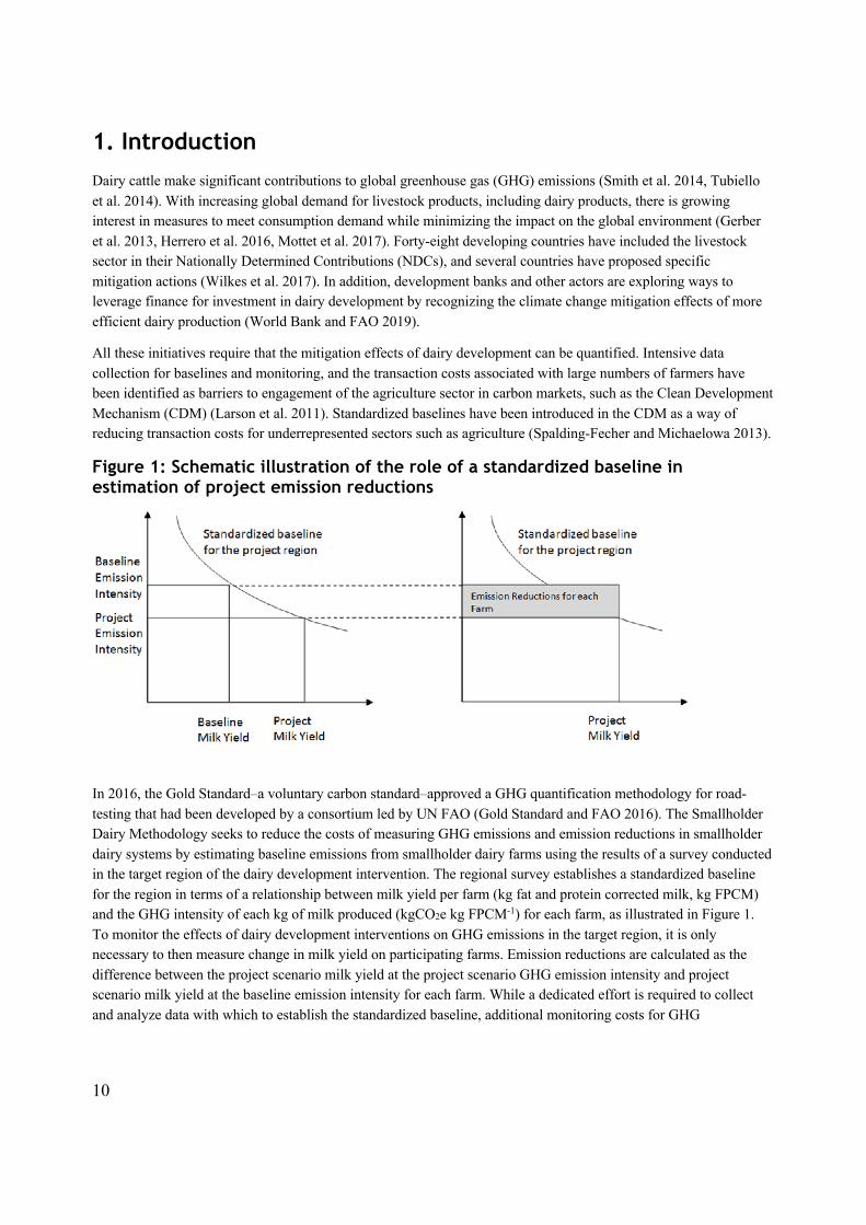
Figure 1: Schematic illustration of the role of a standardized baseline in estimation of project emission reductions

In 2016, the Gold Standard–a voluntary carbon standard–approved a GHG quantification methodology for road-testing that had been developed by a consortium led by UN FAO (Gold Standard and FAO 2016). The Smallholder Dairy Methodology seeks to reduce the costs of measuring GHG emissions and emission reductions in smallholder dairy systems by estimating baseline emissions from smallholder dairy farms using the results of a survey conducted in the target region of the dairy development intervention. The regional survey establishes a standardized baseline for the region in terms of a relationship between milk yield per farm (kg fat and protein corrected milk, kg FPCM) and the GHG intensity of each kg of milk produced (kgCO2e kg FPCM-1) for each farm, as illustrated in Figure 1. To monitor the effects of dairy development interventions on GHG emissions in the target region, it is only necessary to then measure change in milk yield on participating farms. Emission reductions are calculated as the difference between the project scenario milk yield at the project scenario GHG emission intensity and project scenario milk yield at the baseline emission intensity for each farm. While a dedicated effort is required to collect and analyze data with which to establish the standardized baseline, additional monitoring costs for GHG

11

quantification purposes are minimized as monitoring milk yield is a standard practice in dairy development interventions.

The Government of Kenya has proposed a nationally appropriate mitigation action (NAMA) for the dairy sector (State Department of Livestock 2017). Kenya’s Dairy NAMA proposes to use the Smallholder Dairy Methodology to measure GHG emission reductions from dairy development interventions. To test the practical feasibility of the methodology, a pilot baseline survey was conducted in central Kenya, a region dominated by intensive dairy cattle production. The intention is that the field-tested methods can then be replicated in other regions of the country, ultimately providing standardized baselines with nationwide coverage for the dairy NAMA. Similar initiatives are also being developed in other developing countries and these methods may be adopted for use elsewhere.

The descriptive results of the pilot baseline survey were also used as the main data source to estimate dairy cattle characteristics and performance in the intensive dairy production system represented in Kenya’s national GHG inventory (State Department of Livestock 2019). Publishing the data collection methods used and the summary results increases the transparency of the Dairy NAMA Measurement, Reporting and Verification (MRV) system and the national GHG inventory. By documenting the methods used in the Kenya baseline survey, this report can also serve as a reference for similar activities elsewhere.

This report is structured as follows: Section 2 gives an overview of the Smallholder Dairy Methodology’s requirements and the process used to estimate a standardized baseline for one region in Kenya. Section 3 describes the methods used for sampling and data collection. Section 4 describes the methods used to process the data, including treatment of missing values, and preliminary data analysis. Section 5 describes the methods used to transform the data into estimates of parameter values required by the Smallholder Dairy Methodology. Section 6 summarizes the key lessons from the baseline survey and recommendations for future similar initiatives to quantify standardized baselines for dairy GHG mitigation programmes. Appendices present the data collection tool, the main descriptive statistics for the data collected and a comparison of the primary dataset with a dataset containing interpolated missing values, as well as other input data used.

12

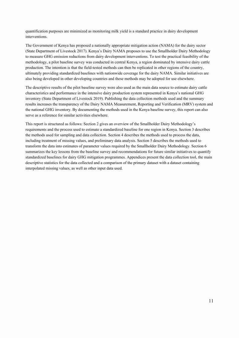
2. Overview of the Smallholder Dairy Methodology requirements and baseline survey process Figure 2 gives an overview of the methodological process for developing the standardized baseline and the corresponding sections in this report. The baseline survey was designed to provide the data needed to quantify GHG intensity of milk production per farm using the methodology set out in the Smallholder Dairy Methodology. The data collection tool used in the survey is shown in Appendix 1. The Smallholder Dairy Methodology requires that the baseline survey should be representative of smallholder dairy farms in the target region and cover production systems that contain at least 80% of smallholder dairy cows in the target region. For this, a sampling strategy is required (see Section 3).

Figure 2. Overview of methodological process and corresponding sections in this report

Once data has been collected and preliminary data analysis completed, the data is used to calculate parameters at three levels:

§ Individual animals: data on several parameters (including milk yield) are used to estimate GHG emissions for each animal present on each farm during the survey, including cows as well as other cattle types, such as heifers, calves, bulls and replacement males;

13

§ Farm emissions: GHG emissions and milk yield are calculated per farm, including GHG emissions from animals on-farm during the survey, emissions from animals that have exited the farm during the year prior to the survey, and emissions from animals kept off-farm for farms that do not maintain sufficient replacement animals to maintain the size of their dairy herd, but excluding surplus males that are not replacements for existing breeding males on the farm;

§ Stratum: For the calculation of off-farm replacement animals and estimation of the standardized baseline, the methodology requires that some parameters are calculated as an average for each type of farm. In the Kenya case, farm types or strata are defined by feeding system, i.e. zero-grazing, mixed stall-fed + grazing (known as ‘semi-zero grazing’), and grazing only feeding systems.

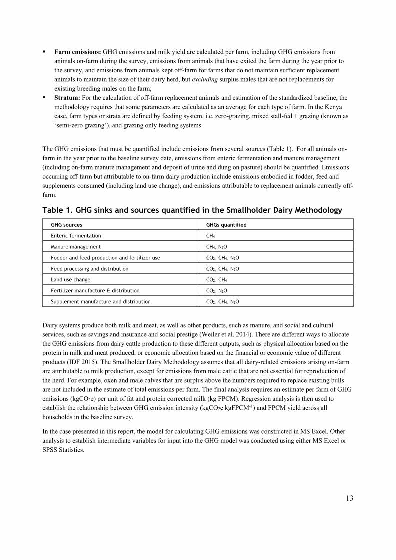
The GHG emissions that must be quantified include emissions from several sources (Table 1). For all animals on-farm in the year prior to the baseline survey date, emissions from enteric fermentation and manure management (including on-farm manure management and deposit of urine and dung on pasture) should be quantified. Emissions occurring off-farm but attributable to on-farm dairy production include emissions embodied in fodder, feed and supplements consumed (including land use change), and emissions attributable to replacement animals currently off-farm.

Table 1. GHG sinks and sources quantified in the Smallholder Dairy Methodology

GHG sources GHGs quantified

Enteric fermentation CH4

Manure management CH4, N2O

Fodder and feed production and fertilizer use CO2, CH4, N2O

Feed processing and distribution CO2, CH4, N2O

Land use change CO2, CH4

Fertilizer manufacture & distribution CO2, N2O

Supplement manufacture and distribution CO2, CH4, N2O

Dairy systems produce both milk and meat, as well as other products, such as manure, and social and cultural services, such as savings and insurance and social prestige (Weiler et al. 2014). There are different ways to allocate the GHG emissions from dairy cattle production to these different outputs, such as physical allocation based on the protein in milk and meat produced, or economic allocation based on the financial or economic value of different products (IDF 2015). The Smallholder Dairy Methodology assumes that all dairy-related emissions arising on-farm are attributable to milk production, except for emissions from male cattle that are not essential for reproduction of the herd. For example, oxen and male calves that are surplus above the numbers required to replace existing bulls are not included in the estimate of total emissions per farm. The final analysis requires an estimate per farm of GHG emissions (kgCO2e) per unit of fat and protein corrected milk (kg FPCM). Regression analysis is then used to establish the relationship between GHG emission intensity (kgCO2e kgFPCM-1) and FPCM yield across all households in the baseline survey.

In the case presented in this report, the model for calculating GHG emissions was constructed in MS Excel. Other analysis to establish intermediate variables for input into the GHG model was conducted using either MS Excel or SPSS Statistics.

14

3. Sampling and data collection

3.1. Methodology requirements The Smallholder Dairy Methodology states that the standardized baseline methodology is applicable under the following conditions:

“(a) In regions where dairy production already occurs on a scale sufficient that a sample survey can quantify baseline management practices to a precision level of 90%±10%;

(b) The survey to determine the standardized baseline covers the different types of dairy farm operations that raise at least 80% of dairy animals in the project region (excluding dairy operations that are not small-scale as defined in footnote 1 above)” (Gold Standard and FAO 2016, p.13).

Applicability condition (a) is intended to ensure that the population of dairy farms is sufficient to enable a representative sample to be taken. The term “baseline management practices” is not well defined. Life Cycle Assessment (LCA) of dairy production in smallholder dairy systems generally finds that enteric methane production is the largest single source of GHG emissions, accounting for 68% to 88% of total CO2e emissions (Weiler et al. 2014, FAO and NZAGRC 2017). Gross energy intake is a key determinant of both enteric fermentation and manure management emissions. In smallholder dairy systems such as in Kenya, gross energy intake is largely driven by animal live weight (LW) and the energy digestibility of feed, which co-determine dry matter intake (DMI). Milk yields may also be a major driver of gross energy intake if it is sufficiently high such that net energy for lactation is a significant proportion of total net energy requirements.

The Smallholder Dairy Methodology refers to guidance on sampling from the CDM.1 That guidance clarifies that where there are multiple parameters to estimate through sampling, the sample size shall be given by the largest sample size of the different parameters required to achieve a precision level of 90%±10%. Appendix 3 provides analysis of the precision achievable for key driving variables with different sample sizes using the survey data from Kenya.

Applicability condition (b) implies that only smallholder dairy farms need be sampled, since the Smallholder Dairy Methodology is not applicable to large-scale, industrial dairy farming operations. Note that if sampling follows this requirement, then the resulting data may not be fully representative of all dairy farms or dairy cows in the target region. This may limit the application of the data to other purposes, e.g. for use in national GHG inventories.

3.2. Sampling strategy Several sources give general guidance on sampling for rural household surveys (e.g. UN DESA 2005). Considering transport and other survey costs, multistage cluster sampling may be a cost-effective sampling method. With multistage cluster sampling, enumeration areas (e.g. wards, villages) are selected randomly from within the target region, and clusters of households (e.g. households in the same village) are selected in each enumeration area. The multistage sampling procedure employed to select representative locations (enumeration areas) and households in the pilot baseline survey in Kenya is elaborated below.

Stage 1: Identification of the target population: For the pilot baseline survey, the target population was identified as households with dairy cattle in the intensive production region of Kenya. The intensive production region had

1 https://cdm.unfccc.int/Reference/Standards/meth/meth_stan05.pdf

15

been identified by a previous study of dairy production in Kenya by FAO (FAO and NZAGRC 2017). The counties in this region are: Embu, Kiambu, Kirinyaga, Meru, Murang’a, Nakuru, Nyandarua and Nyeri.2

Stage 2: Sampling of enumeration areas: Considering the resources available for the pilot baseline survey, within each county it was planned to sample households clustered in 41 enumeration areas, with 10 households per cluster. Since there were no prior lists of households with dairy cattle, enumeration areas were chosen by randomly selecting locations within each county using a script to perform random selection of locations in GIS after blocking out forest and urban areas. The selected points were moved to the nearest village, school, crossroads or other identified location. Twelve points were selected in each county, with two points being used as replacement enumeration areas in case any of the selected enumeration areas had insufficient numbers of dairy producing households. Prior to the survey, the location of each site and the presence of dairy production in the nearest village was verified, and contacts with the resident administrative officials were made.

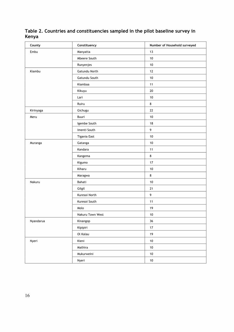
Stage 3: Random sampling of households: Since there are no prior lists of households with dairy cattle in each village or enumeration area, a transect sampling method was used (Staal et al. 2002). Discussions with the local administration were held to produce a hand-drawn map of the village and identify key landmarks (e.g. river, school, church etc.) on each side of the village. Pairs of landmarks were selected and straight lines (transects) were drawn between them. One transect was chosen at random, and the enumeration team walked along the transect sampling every fifth household along the transect, until 10 households with dairy cows had been interviewed. If a household was selected that does not have dairy cows, then the enumeration team proceeded to the next sampled household (i.e. 5 households later). If a transect was completed and still 10 households had not been interviewed, another transect was randomly selected and household sampling repeated in the same manner. In the pilot baseline survey, 429 households were sampled at locations shown in Table 2.

2 This grouping of counties differs slightly from the counties identified as having ‘intensive production systems’ in Kenya’s Tier 2 dairy cattle GHG inventory (State Department of Livestock 2019).

16

Table 2. Countries and constituencies sampled in the pilot baseline survey in Kenya

County Constituency Number of Household surveyed

Embu Manyatta 13

Mbeere South 10

Runyenjes 10

Kiambu Gatundu North 12

Gatundu South 10

Kiambaa 11

Kikuyu 20

Lari 10

Ruiru 8

Kirinyaga Gichugu 22

Meru Buuri 10

Igembe South 18

Imenti South 9

Tigania East 10

Muranga Gatanga 10

Kandara 11

Kangema 8

Kigumo 17

Kiharu 10

Maragwa 8

Nakuru Bahati 10

Gilgil 21

Kuresoi North 9

Kuresoi South 11

Molo 19

Nakuru Town West 10

Nyandarua Kinangop 36

Kipipiri 17

Ol Kalau 19

Nyeri Kieni 10

Mathira 10

Mukurweini 10

Nyeri 10

17

3.3. Data collection

3.3.1. Data collection tool Appendix 1 shows the data collection tool used in the pilot baseline survey. Appendix 2 summarizes which of the parameters required by the Smallholder Dairy Methodology are derived from which sections of the survey tool.

In particular, it is worth noting that the definition of animal sub-categories used in the survey tool differs from more common categorizations used in Kenya. The survey tool codings give 13 animal sub-categories, which is more than is usually used in household surveys of dairy production. The reasons are:

(a) sub-dividing adult males in bulls and oxen is used to select the appropriate value for the coefficient for growth (C) in the IPCC model, which varies between castrated and intact males;

(b) subdividing cows into lactating, dry and lactating in-calf cows is used together with other information on milk production and calving interval to ensure a more accurate estimate of the proportion of cows that were pregnant in the year;

(c) subdividing heifers into those that are and are not in-calf is useful to correctly apply the coefficient for pregnancy (Cp) to heifers that have not yet calved.

3.3.2. Enumerator training A team of enumerators was formed that consisted of professionals and graduate students with animal or veterinary science or social science background. All had previous experience of conducting household surveys. Three survey team leaders with prior experience of managing survey teams in the field and quality control were also in the team. A two-day training course was provided, with the first day covering every detail of the sampling procedure and survey tool, and the second day involving trial data collection with dairy farming households.

3.3.3. Selection of respondents Because the survey requires in-depth familiarity with the dairy cattle raising practices of the household, the questionnaire must be answered by an adult household member with some responsibility for dairy cattle keeping. The questions on the introductory page of the survey tool (Appendix 1) aim to ensure that eligible household members were identified. The respondent may be the household head, spouse or another adult household member. Hired workers may only be the main respondent if the household head or spouse has agreed. If the household head is not involved in dairy cattle raising, enumerators were instructed to identify another eligible household member with more specific knowledge of household dairy management practices. The respondent eventually selected responded to the questionnaire.

18

4. Preliminary data analysis

4.1. General procedures The raw data was entered into SPSS. Data cleaning involved checks for transcription errors (e.g. values that were not present in the item codings, implausible parameter values), and cross-checks of the categorization of each animal by sub-category against reported age, live weight (LW), calving and lactation history. In particular, the age of animals was used to confirm that the recorded age of each animal is within the age range for the definition of each animal sub-category, and to check that the pregnancy, birth or lactation status of each type of cow corresponds to the definition for each sub-category of cow. Outlier parameter values were cross-checked against the original survey forms, and in a small number of cases the respondent was re-contacted in order to cross-check reported values or replace missing values.

4.2. Survey-specific procedures The definition of dairy farm strata used in analysis of the baseline survey data was determined ex-post on the basis of data collected by the survey tool on feeding management for productive females in each household (Table 4.2 in Appendix 1). Specific definitions used to allocate households to a feeding system were:

§ Zero-grazing system: All productive females and replacement heifers are raised in zero-grazing systems in both dry and wet seasons. In some cases, male animals may be grazed, but since the intensiveness of production practices for females is expected to be the main determinant of milk production, the grazing system for females was used as the defining characteristic.

§ Semi-zero grazing system: Some productive females or replacement heifers graze for some part of the year. § Grazing system: All productive females and replacement heifers graze 100% of the time in both wet and dry

seasons.

This information is given in responses to Question 4.2 in the survey tool (see Appendix 1), which was analysed prior to analysis of other survey data so that each farm was coded by feeding system prior to further analysis.

4.3. Dealing with missing values There can be many reasons for incomplete data. Possible reasons include:

§ Omissions when filling in questionnaire forms § Lack of understanding or knowledge on the part of the respondent § Requesting information in units or to a level of detail that farmers are unaccustomed to measuring § Requesting information on too long a recall period § Refusal to respond by the respondent, e.g. due to fatigue or other reasons.

Some of these reasons can be avoided, for example, by

§ Testing the survey tool in a small-scale pilot § Ensuring that survey enumerators are properly trained in both interviewing and documenting responses § Ensuring that respondents have been regularly involved in farm dairy operations over the year prior to the

survey § Ensuring timely inspection of completed survey forms in the field, so that any omissions can be detected and

follow-up interviews made § Taking direct measurements, e.g. heart girth measurements, age estimation using dentition.

19

However, some of causes of missing data cannot be avoided. For example, resource limitations mean that it would not be possible to directly measure several parameters across a large number of households. In the pilot baseline survey, for example, enumerators were instructed to select one animal of each type present on the farm for heart girth measurement. This saved time but resulted in a large number of missing values for the live weight of animals that were not measured. Another example might be where cows are frequently purchased as mature animals, and the new owners may not know the age, parity, calving interval or dates of last calving for these animals.

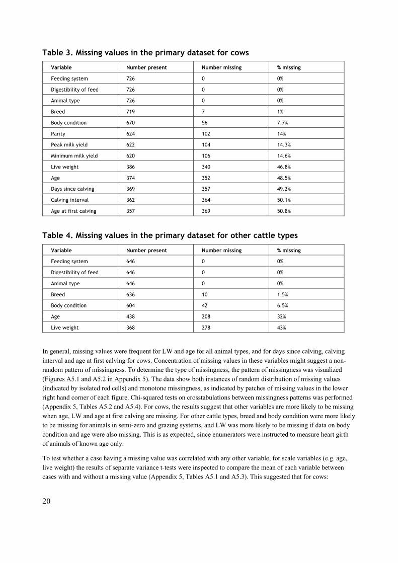
Thirty-two cases (i.e. households) were deleted that had missing values for animal type, since it would not be plausible to impute values for other parameters if animal type is unknown, leaving a sample of 397 households for data analysis. Missing value analysis in SPSS Statistics was used to diagnose the extent, patterns and mechanisms of missing data in the primary dataset. First, the presence or absence of missing data were tabulated by each of the key parameters. This was done separately for cows (Table 3) and for other cattle types (Table 4), because variables such as age at first calving or milk yield are by definition ‘missing’ for other animal types. For example, results for cows (Table 3) show that among 12 variables, there were no missing values for feeding system type, animal type or feed digestibility, and few missing values for breed or body condition, but 14-51% of cases had missing values for other variables. Overall, for cows 90% of cases had at least one missing value, with 28% of all values missing. For other cattle types, age and/or live weight (LW) were missing in 32%-43% of cases, and 53% of cases had at least one missing value.

20

Table 3. Missing values in the primary dataset for cows

Variable Number present Number missing % missing

Feeding system 726 0 0%

Digestibility of feed 726 0 0%

Animal type 726 0 0%

Breed 719 7 1%

Body condition 670 56 7.7%

Parity 624 102 14%

Peak milk yield 622 104 14.3%

Minimum milk yield 620 106 14.6%

Live weight 386 340 46.8%

Age 374 352 48.5%

Days since calving 369 357 49.2%

Calving interval 362 364 50.1%

Age at first calving 357 369 50.8%

Table 4. Missing values in the primary dataset for other cattle types

Variable Number present Number missing % missing

Feeding system 646 0 0%

Digestibility of feed 646 0 0%

Animal type 646 0 0%

Breed 636 10 1.5%

Body condition 604 42 6.5%

Age 438 208 32%

Live weight 368 278 43%

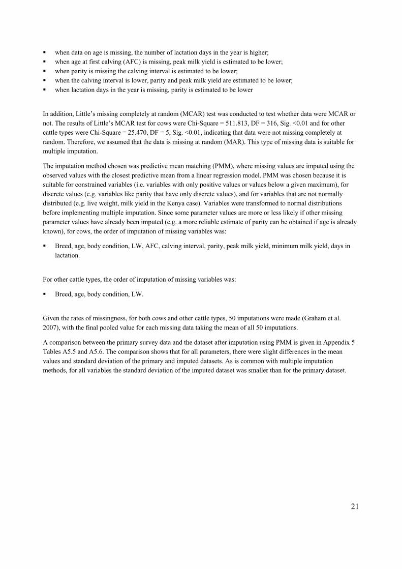
In general, missing values were frequent for LW and age for all animal types, and for days since calving, calving interval and age at first calving for cows. Concentration of missing values in these variables might suggest a non-random pattern of missingness. To determine the type of missingness, the pattern of missingness was visualized (Figures A5.1 and A5.2 in Appendix 5). The data show both instances of random distribution of missing values (indicated by isolated red cells) and monotone missingness, as indicated by patches of missing values in the lower right hand corner of each figure. Chi-squared tests on crosstabulations between missingness patterns was performed (Appendix 5, Tables A5.2 and A5.4). For cows, the results suggest that other variables are more likely to be missing when age, LW and age at first calving are missing. For other cattle types, breed and body condition were more likely to be missing for animals in semi-zero and grazing systems, and LW was more likely to be missing if data on body condition and age were also missing. This is as expected, since enumerators were instructed to measure heart girth of animals of known age only.

To test whether a case having a missing value was correlated with any other variable, for scale variables (e.g. age, live weight) the results of separate variance t-tests were inspected to compare the mean of each variable between cases with and without a missing value (Appendix 5, Tables A5.1 and A5.3). This suggested that for cows:

21

§ when data on age is missing, the number of lactation days in the year is higher; § when age at first calving (AFC) is missing, peak milk yield is estimated to be lower; § when parity is missing the calving interval is estimated to be lower; § when the calving interval is lower, parity and peak milk yield are estimated to be lower; § when lactation days in the year is missing, parity is estimated to be lower

In addition, Little’s missing completely at random (MCAR) test was conducted to test whether data were MCAR or not. The results of Little’s MCAR test for cows were Chi-Square = 511.813, DF = 316, Sig. <0.01 and for other cattle types were Chi-Square = 25.470, DF = 5, Sig. <0.01, indicating that data were not missing completely at random. Therefore, we assumed that the data is missing at random (MAR). This type of missing data is suitable for multiple imputation.

The imputation method chosen was predictive mean matching (PMM), where missing values are imputed using the observed values with the closest predictive mean from a linear regression model.PMM was chosen because it is suitable for constrained variables (i.e. variables with only positive values or values below a given maximum), for discrete values (e.g. variables like parity that have only discrete values), and for variables that are not normally distributed (e.g. live weight, milk yield in the Kenya case). Variables were transformed to normal distributions before implementing multiple imputation. Since some parameter values are more or less likely if other missing parameter values have already been imputed (e.g. a more reliable estimate of parity can be obtained if age is already known), for cows, the order of imputation of missing variables was:

§ Breed, age, body condition, LW, AFC, calving interval, parity, peak milk yield, minimum milk yield, days in lactation.

For other cattle types, the order of imputation of missing variables was:

§ Breed, age, body condition, LW.

Given the rates of missingness, for both cows and other cattle types, 50 imputations were made (Graham et al. 2007), with the final pooled value for each missing data taking the mean of all 50 imputations.

A comparison between the primary survey data and the dataset after imputation using PMM is given in Appendix 5 Tables A5.5 and A5.6. The comparison shows that for all parameters, there were slight differences in the mean values and standard deviation of the primary and imputed datasets. As is common with multiple imputation methods, for all variables the standard deviation of the imputed dataset was smaller than for the primary dataset.

22

5. Calculation of GHG emissions Preliminary data analysis described in the previous section created a full dataset of the parameters required for estimating GHG emissions from each animal and thus each farm surveyed. This section explains the methods used to transform the raw data into estimates of GHG emissions and milk yields per animal and per farm.

5.1. Quantification of individual animal GHG emissions and milk yield GHG emissions attributable to each animal present on the farm during the year prior to the survey include:

§ (1) Methane emissions from enteric fermentation § (2) Methane emissions from manure management § (3) Nitrous oxide emissions from manure management and dung and urine deposited on pasture § (4) Emissions embodied in feed consumed on farm. Estimates from (1)-(4) are then used to estimate:

§ (5) Emissions from animals that were present on the farm for only part of the year, and § (6) Emissions from replacement animals that are not kept on the farm.

5.1.1. Enteric fermentation emissions The method required by the Smallholder Dairy Methodology for quantification of enteric fermentation emissions is the IPCC Tier 2 approach. The specific IPCC equations are not presented here, but can be found in the IPCC Guidelines (IPCC 2006). Table 5 shows the variables for which data is required. The baseline survey data indicated that only 2 out of 1400 dairy cattle surveyed did any work during the year, so net energy for work was not calculated.3 Each of the following sub-sections describes how the parameters required for estimation of enteric fermentation emissions using the IPCC Tier 2 model can be obtained from analysis of the baseline survey data. Note that because net energy for maintenance is an input into the estimation of net energy for activity and net energy for pregnancy, it was calculated first.

3 If any type of dairy cattle do significant amounts of work, the IPCC guidelines should be followed to estimate net energy for work.

23

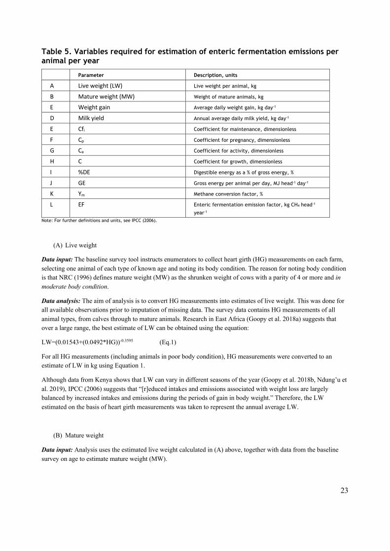
Table 5. Variables required for estimation of enteric fermentation emissions per animal per year

Parameter Description, units

A Live weight (LW) Live weight per animal, kg

B Mature weight (MW) Weight of mature animals, kg

E Weight gain Average daily weight gain, kg day-1

D Milk yield Annual average daily milk yield, kg day-1

E Cfi Coefficient for maintenance, dimensionless

F Cp Coefficient for pregnancy, dimensionless

G Ca Coefficient for activity, dimensionless

H C Coefficient for growth, dimensionless

I %DE Digestible energy as a % of gross energy, %

J GE Gross energy per animal per day, MJ head-1 day-1

K Ym Methane conversion factor, %

L EF Enteric fermentation emission factor, kg CH4 head-1

year-1 Note: For further definitions and units, see IPCC (2006).

(A) Live weight

Data input: The baseline survey tool instructs enumerators to collect heart girth (HG) measurements on each farm, selecting one animal of each type of known age and noting its body condition. The reason for noting body condition is that NRC (1996) defines mature weight (MW) as the shrunken weight of cows with a parity of 4 or more and in moderate body condition.

Data analysis: The aim of analysis is to convert HG measurements into estimates of live weight. This was done for all available observations prior to imputation of missing data. The survey data contains HG measurements of all animal types, from calves through to mature animals. Research in East Africa (Goopy et al. 2018a) suggests that over a large range, the best estimate of LW can be obtained using the equation:

LW=(0.01543+(0.0492*HG))-0.3595 (Eq.1)

For all HG measurements (including animals in poor body condition), HG measurements were converted to an estimate of LW in kg using Equation 1.

Although data from Kenya shows that LW can vary in different seasons of the year (Goopy et al. 2018b, Ndung’u et al. 2019), IPCC (2006) suggests that “[r]educed intakes and emissions associated with weight loss are largely balanced by increased intakes and emissions during the periods of gain in body weight.” Therefore, the LW estimated on the basis of heart girth measurements was taken to represent the annual average LW.�

(B) Mature weight

Data input: Analysis uses the estimated live weight calculated in (A) above, together with data from the baseline survey on age to estimate mature weight (MW).

24

Data analysis: The aim of analysis is to estimate the MW for male and female cattle in each stratum (e.g. feeding system). For females, MW is defined as the shrunken body weight of cows after their 4th parity in moderate body condition, and shrunken body weight is estimated as live weight multiplied by 0.96 (NRC 1996). Where there is no statistically significant difference between strata, or where the sample size is too small (e.g. for castrated oxen, which were uncommon on dairy farms in the baseline survey) a single value was used in the GHG calculations for all strata. For example, given very small samples of bulls (n=47) and oxen (n=5), after excluding males in poor body condition, the top quartile of LW was used to estimate MW. For cows, there were no statistically significant differences between mean live weights of mature cows in different feeding systems, so a single estimate of MW was used.

(C) Daily weight gain

Data input: Analysis used the estimated LW calculated in (A) above, and data from the baseline survey on animal type and age to estimate daily weight gain (WG).

Data analysis: The aim of analysis is to estimate daily weight gain for each type of growing animal (i.e. male and female calves, heifers and growing males). Following IPCC (2006), we assume that weight gain for adult cows and males is equal to zero. Daily weight gain is used to estimate net energy for growth for each animal type.

Calf daily weight gain is expected to be higher at younger age, gradually decreasing as age increases, and many calves in the survey were less than 6 months old. So estimating daily weight gain by dividing weight gain since birth by the number of days since birth for each animal would overestimate annual average daily weight gain for calves that had been alive for less than a year. Therefore, annual average daily weight gain was estimated for each sub-category of growing animal in each stratum.

Using data on LW calculated in (A) above for growing cattle types (i.e. male and female calves, heifers and growing males), the dataset was divided by stratum (i.e. feeding system). Survey data on age in months was converted to age in days. A best-fit regression equation was established between age in days and LW for male and female calves separately. The resulting equations were used to estimate LW for the typical animal of each sex for each age group of growing animal. From the estimate of LW at each age, average daily weight gain (i.e. ΔLW) during the period representing the age range of each animal type was estimated.

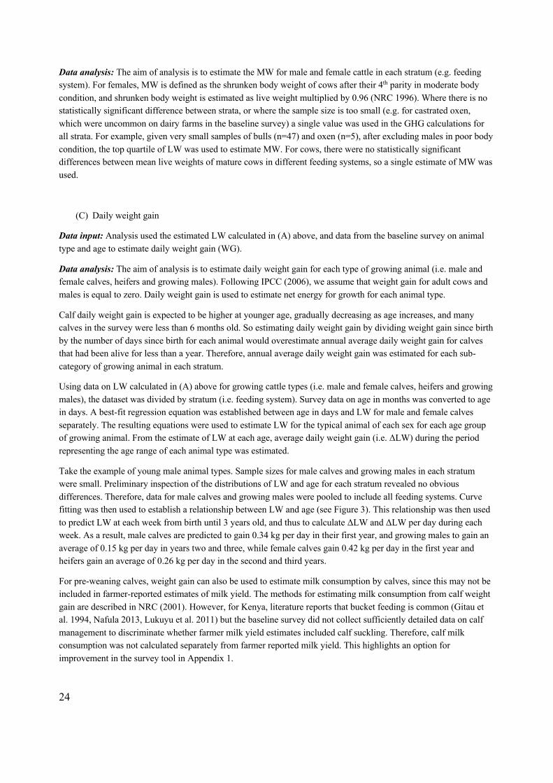
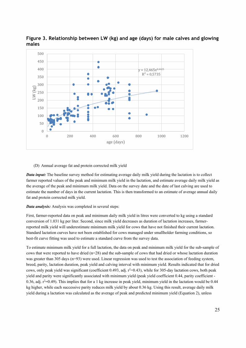
Take the example of young male animal types. Sample sizes for male calves and growing males in each stratum were small. Preliminary inspection of the distributions of LW and age for each stratum revealed no obvious differences. Therefore, data for male calves and growing males were pooled to include all feeding systems. Curve fitting was then used to establish a relationship between LW and age (see Figure 3). This relationship was then used to predict LW at each week from birth until 3 years old, and thus to calculate ΔLW and ΔLW per day during each week. As a result, male calves are predicted to gain 0.34 kg per day in their first year, and growing males to gain an average of 0.15 kg per day in years two and three, while female calves gain 0.42 kg per day in the first year and heifers gain an average of 0.26 kg per day in the second and third years.

For pre-weaning calves, weight gain can also be used to estimate milk consumption by calves, since this may not be included in farmer-reported estimates of milk yield. The methods for estimating milk consumption from calf weight gain are described in NRC (2001). However, for Kenya, literature reports that bucket feeding is common (Gitau et al. 1994, Nafula 2013, Lukuyu et al. 2011) but the baseline survey did not collect sufficiently detailed data on calf management to discriminate whether farmer milk yield estimates included calf suckling. Therefore, calf milk consumption was not calculated separately from farmer reported milk yield. This highlights an option for improvement in the survey tool in Appendix 1.

25

Figure 3. Relationship between LW (kg) and age (days) for male calves and glowing males

(D) Annual average fat and protein corrected milk yield

Data input: The baseline survey method for estimating average daily milk yield during the lactation is to collect farmer reported values of the peak and minimum milk yield in the lactation, and estimate average daily milk yield as the average of the peak and minimum milk yield. Data on the survey date and the date of last calving are used to estimate the number of days in the current lactation. This is then transformed to an estimate of average annual daily fat and protein corrected milk yield.

Data analysis: Analysis was completed in several steps:

First, farmer-reported data on peak and minimum daily milk yield in litres were converted to kg using a standard conversion of 1.031 kg per liter. Second, since milk yield decreases as duration of lactation increases, farmer-reported milk yield will underestimate minimum milk yield for cows that have not finished their current lactation. Standard lactation curves have not been established for cows managed under smallholder farming conditions, so best-fit curve fitting was used to estimate a standard curve from the survey data.

To estimate minimum milk yield for a full lactation, the data on peak and minimum milk yield for the sub-sample of cows that were reported to have dried (n=28) and the sub-sample of cows that had dried or whose lactation duration was greater than 305 days (n=93) were used. Linear regression was used to test the association of feeding system, breed, parity, lactation duration, peak yield and calving interval with minimum yield. Results indicated that for dried cows, only peak yield was significant (coefficient 0.493, adj. r2=0.43), while for 305-day lactation cows, both peak yield and parity were significantly associated with minimum yield (peak yield coefficient 0.44, parity coefficient -0.36, adj. r2=0.49). This implies that for a 1 kg increase in peak yield, minimum yield in the lactation would be 0.44 kg higher, while each successive parity reduces milk yield by about 0.36 kg. Using this result, average daily milk yield during a lactation was calculated as the average of peak and predicted minimum yield (Equation 2), unless

y=12,465x0,4425

R²=0,5735

0

50

100

150

200

250

300

350

400

450

500

0 200 400 600 800 1000 1200

LW(kg)

age(days)

26

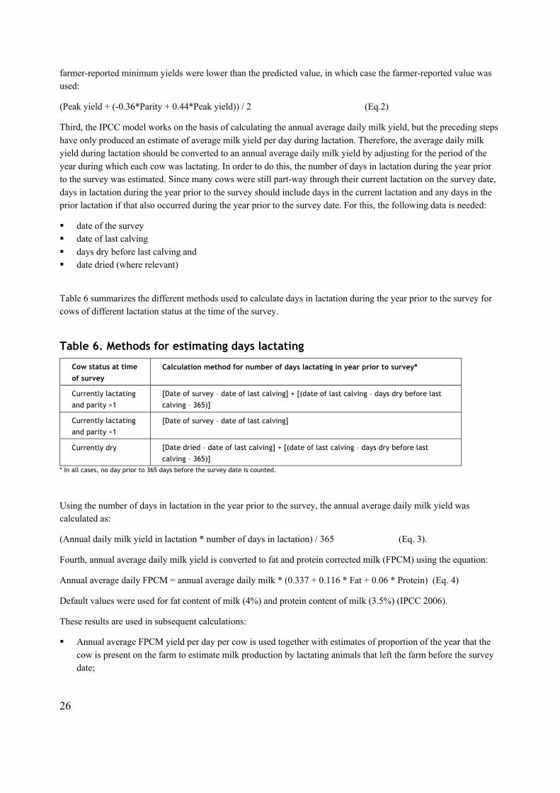
farmer-reported minimum yields were lower than the predicted value, in which case the farmer-reported value was used:

(Peak yield + (-0.36*Parity + 0.44*Peak yield)) / 2 (Eq.2)

Third, the IPCC model works on the basis of calculating the annual average daily milk yield, but the preceding steps have only produced an estimate of average milk yield per day during lactation. Therefore, the average daily milk yield during lactation should be converted to an annual average daily milk yield by adjusting for the period of the year during which each cow was lactating. In order to do this, the number of days in lactation during the year prior to the survey was estimated. Since many cows were still part-way through their current lactation on the survey date, days in lactation during the year prior to the survey should include days in the current lactation and any days in the prior lactation if that also occurred during the year prior to the survey date. For this, the following data is needed:

§ date of the survey § date of last calving § days dry before last calving and § date dried (where relevant)

Table 6 summarizes the different methods used to calculate days in lactation during the year prior to the survey for cows of different lactation status at the time of the survey.

Table 6. Methods for estimating days lactating

Cow status at time of survey

Calculation method for number of days lactating in year prior to survey*

Currently lactating

and parity >1

[Date of survey – date of last calving] + [(date of last calving – days dry before last

calving – 365)]

Currently lactating

and parity =1 [Date of survey – date of last calving]

Currently dry [Date dried – date of last calving] + [(date of last calving – days dry before last

calving – 365)] * In all cases, no day prior to 365 days before the survey date is counted.

Using the number of days in lactation in the year prior to the survey, the annual average daily milk yield was calculated as:

(Annual daily milk yield in lactation * number of days in lactation) / 365 (Eq. 3).

Fourth, annual average daily milk yield is converted to fat and protein corrected milk (FPCM) using the equation:

Annual average daily FPCM = annual average daily milk * (0.337 + 0.116 * Fat + 0.06 * Protein) (Eq. 4)

Default values were used for fat content of milk (4%) and protein content of milk (3.5%) (IPCC 2006).

These results are used in subsequent calculations:

§ Annual average FPCM yield per day per cow is used together with estimates of proportion of the year that the cow is present on the farm to estimate milk production by lactating animals that left the farm before the survey date;

27

§ Annual average FPCM yield per day per cow is multiplied by the proportion of the year that each animal was present on the farm to estimate annual FPCM per animal;

§ The sum of annual FPCM per animal for all animals on the same farm is calculated to estimate annual FPCM per farm.

(E) Coefficient for maintenance (Cfi)

Data input: IPCC (2006) gives default values for the coefficient for maintenance (Cfi) for bulls, lactating cows and non-lactating cows. The IPCC default value for maintenance is 20% higher for lactating than for non-lactating cows. A value for Cfi was calculated for lactating cows that is weighted by the proportion of the year lactating. The IPCC default value for bulls can be used as given in IPCC (2006). For other female cattle (e.g. heifers and female calves), the value for non-lactating cows (0.322) is used. For other male cattle (e.g. growing males and male calves), the value for intact bulls (0.370) is used.

Data analysis: For cows, days in lactation were estimated in (D) above using baseline survey data for each cow on the date of the survey, date of last calving and (where relevant) date dried. The IPCC default value for Cfi for non-lactating cows is 0.322 and for lactating cows is 0.386. By weighting the coefficient by the proportion of the year spent lactating, the baseline survey derived a mean value for Cfi of 0.372 (s.d. 0.010).

(F) Coefficient for pregnancy (Cp)

Data input: For productive cows, baseline data on date of last calving and calving interval is used to estimate the number of days in the year that each animal was pregnant. A coefficient for pregnancy (Cp) is also applied to pregnant heifers.

Data analysis: The IPCC 2006 default value for Cp (i.e. 0.1) is an annualized estimate assuming a pregnancy of 281 days. It is normally applied together with an estimate of the % of cows giving birth in the year. However, the baseline survey collected finer resolution data on the number of days pregnant during the year prior to the survey, which may be considerably less than 281 days. Therefore, the aim of analysis is the adjust the coefficient for the number of days pregnant during the year.

The number of days pregnant during the year prior to the survey was calculated for each cow using the date of the survey, the date of last calving and assuming 281 days pregnancy:

Date pregnancy began = date of last calving – 281.

If (date pregnancy began – 1 year prior to the date of survey) >0, then days pregnant in the year = (date of last calving - 1 year prior to the date of survey).

If (date pregnancy began – 1 year prior to the date of survey) <0, then days pregnant in the year = 0.

Cp is then calculated as (days pregnant in the year/281) * 0.1.

The resulting mean value for Cp for cows was 0.06 (s.d. 0.03). For pregnant heifers, the IPCC default value was used (i.e., 0.1).

28

(G) Coefficient for activity (Ca)

Data inputs: The IPCC gives default values for the coefficient for activity (Ca) based on feeding situation (i.e., stall feeding, grazing in confined pasture and extensive grazing). The IPCC default values for Ca are 0 for no grazing, 0.17 for confined grazing and 0.36 for extensive grazing. However, no quantitative definition of these feeding situations is given in the IPCC Guidelines. Ca is estimated following equations given in NRC (2001), which consider animal LW and distance travelled.

Data analysis: NRC (2001) suggests that there are two components to net energy for activity: a maintenance energy requirement for walking and a maintenance energy requirement for eating activity. NRC (2001) proposes a value of 0.0012 Mcal per kg body weight for energy associated with eating, and 0.00045 Mcal/kg BW per km distance of walking in flat areas. Mcal was converted to MJ by multiplying by 4.1868. Thus, assuming a cow body weight of 360 kg, the IPCC default of 0.17 for cattle grazing confined areas would apply to a cow walking 3.7 km per day and the value of 0.36 for extensive grazing would imply a distance on flat terrain of more than 12 km per day.

The baseline survey data was analysed as follows:

Annual average km walked per day = (km in wet season * (months of wet season/12)) + (km in dry season * (months in dry season/12)) (Eq. 5)

If the proportion of DMI per day obtained from grazing >0, then:

Ca = ((0.00045*LW*annual average km per day)+(0.0012*LW)*4.1868)/NEm (Eq. 6)

where NEm is net energy for maintenance, calculated using IPCC (2006) Equation 10.3.

If the proportion of DMI per day obtained from grazing = 0, then:

Ca = ((0.00045*LW*annual average km per day) *4.1868)/NEm (Eq. 7)

The resulting average values for Ca were 0.001 in the zero-grazing system (due to a small number of males and replacement animals that were not 100% stall fed); 0.04 in the mixed system; and 0.06 in the grazing system. The baseline survey in Kenya was conducted in a relatively high population density area. More than 70% of sample households operated stall feeding systems for adult and replacement females. Even where there was a mixed stall + grazing system or a fully grazing system, distances estimated by farmers to and from the grazing site each day were small in both wet and dry seasons, with an annual average distance walked per day of 0.55 km in the mixed system and 1 km in the grazing system. Moreover, of those households in mixed or grazing systems, 55% reported tethering at least some animals when grazing. In the mixed and grazing systems, the average animal obtained only 30% and 34% of required DMI through grazing in each system, respectively. Taken together, this suggests that even in mixed and grazing systems in the survey area, most animals obtain a limited proportion of DMI from grazing, and a lower average value for Ca than the IPCC default values for grazing animals is justified.

(H) Coefficient for growth

Data input: Coefficients for growth used the IPCC default values, i.e. 0.8 for all females, 1.0 for castrated males and 1.2 for bulls. The default value for bulls was applied to growing males, and male calves as well as intact adult males.

29

(I) Feed intake and feed energy digestibility

Data input: Baseline survey data on the mass of feed (including roughage, concentrates and organic or inorganic supplements fed) fed to each animal type in each farm is the main input data. In addition, analysis requires the following inputs:

§ Feed unit conversions to kg: Farmers use a variety of units to transport roughage harvest and to feed animals (e.g. debe, wheelbarrow loads, kasuku cans etc). Conversions to kg were obtained from the literature and from expert judgement.

§ Dry matter conversion factors: Feeds reported in the baseline survey include fresh weight and dried fodders, both of which contain moisture. Weights must be converted to dry matter weights.

§ Feed digestibility: Feed digestibility values were not measured in the survey, but were derived from the literature for Kenya, East Africa (where Kenya data are unavailable) or from Feedipedia (where East Africa data are unavailable). At the same time, feed crude protein content (CP%) estimates were obtained for use in the N2O manure management emission estimates.

Dry matter content and feed digestibility values were obtained from scientific publications based on studies conducted in Kenya, the ILRI feed database,4 and from an East Africa regional feed table (Laswai et al. 2013) and are presented in Appendix 6 Table A6.1.

Data analysis: The aim of analysis is to estimate the average feed energy digestibility of the total feed basket for each animal in the baseline survey. For analysis, the following steps were followed:

§ (1) Convert baseline survey feed units into kg; § (2) Convert kg fresh and dry feed into kg DM;

(3) Using baseline survey data on the types of animals fed each type of feed in the wet and dry seasons, estimate the total volume of each type of feed available to each animal on each farm in each season. If the survey indicated that the type of feed was fed to all animal types, then the total available feed was divided by the number of animals present on the farm; if the survey indicated that the feed was fed to specific animal types, the total volume available was divided by the number of animals of that type present on the farm.

(4) Estimate the total amount of each type of feed available per animal per day in each season and then estimate the average annual daily total amount available per animal weighted by the lengths of the wet and dry seasons.

(5) Using data on LW of each animal and digestibility of available feed per animal, apply the appropriate IPCC equations to estimate DMI requirements for each animal (IPCC 2006 Vol. 4 Ch. 10 Equations 10.17-20.18. For growing cattle, a NEma value of 5.0 was assumed).

(6) Compare the estimated DMI requirements with the estimated DM feed available (DMA). If necessary, adjustments are made as follows:

a. If estimated DMA is > DMI, then it is assumed that intake from grazing equals zero. If the survey data reports that grazing animals are tethered, this is a reasonable assumption. Check that feed and supplement feeding rates and roughage:concentrate ratios are reasonable. Taking feed and supplement volumes as fixed, adjust the volume of roughage fed so that the proportion of each roughage type in the total ration is the same as reported by farmers, and the total sum of roughage, concentrate and supplement equals estimated DMI requirements.

4 https://feedsdatabase.ilri.org/

30

b. If estimated DMA is < DMI, then assume that the remaining intake requirement is met through grazing. Cross-check this assumption against the baseline survey data on the proportion of time spent grazing in each season. Where this assumption is inappropriate (e.g. for animals kept under zero-grazing), adjust the total volume of roughage available in proportion to their availability as reported by farmers such that DMA=DMI.

(7) Once the composition of the total ration has been estimated, multiply the dry matter weight of each type of feed consumed by its energy digestibility and calculate the weighted average feed digestibility of the total ration consumed.

The resulting estimated diet composition and average annual feed digestibility is shown in Appendix 6 (Tables A6.2 – A6.5). Although this method of estimating feed intake has many shortcomings, because the volumes of each type of feed consumed will also be used to estimate the emissions from feed production, it is important that the estimated volumes are biologically feasible.

(J) Calculate gross energy

Data input: The parameter values calculated in the preceding subsections are the inputs into the IPCC equations for estimating gross energy (GE) intake (IPCC 2006, Eq. 10.14-10.16).

Data analysis: The aim of analysis is to estimate GE for each animal present on each farm. The parameter and coefficient values previously calculated are used together with the IPCC equations to estimate GE.

(K) Methane conversion factor

Data input: The IPCC default value for the methane conversion factor (Ym) of 6.5% was used for all cattle types.

(L) Calculate enteric fermentation emission factors

Data input: Estimated GE and data on entry and exit of animals from each farm are used together with the IPCC equations to estimate an annualized emission factor for each animal.

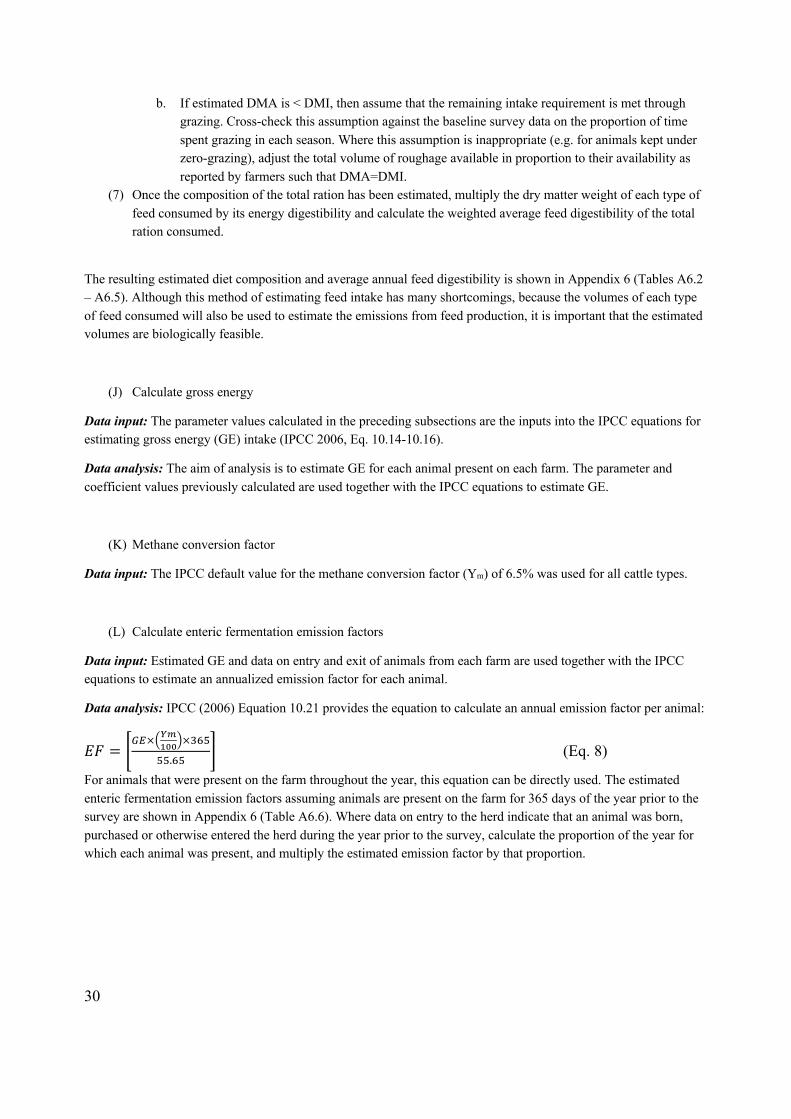
Data analysis: IPCC (2006) Equation 10.21 provides the equation to calculate an annual emission factor per animal:

!" = $%&×()*+,,-×./000./0 2 (Eq. 8)

For animals that were present on the farm throughout the year, this equation can be directly used. The estimated enteric fermentation emission factors assuming animals are present on the farm for 365 days of the year prior to the survey are shown in Appendix 6 (Table A6.6). Where data on entry to the herd indicate that an animal was born, purchased or otherwise entered the herd during the year prior to the survey, calculate the proportion of the year for which each animal was present, and multiply the estimated emission factor by that proportion.

31

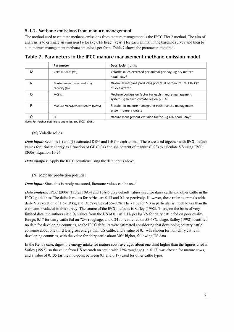
5.1.2. Methane emissions from manure management The method used to estimate methane emissions from manure management is the IPCC Tier 2 method. The aim of analysis is to estimate an emission factor (kg CH4 head-1 year-1) for each animal in the baseline survey and then to sum manure management methane emissions per farm. Table 7 shows the parameters required.

Table 7. Parameters in the IPCC manure management methane emission model


M Volatile solids (VS) Volatile solids excreted per animal per day, kg dry matter

head-1 day-1

N Maximum methane producing capacity (Bo)

Maximum methane producing potential of manure, m3 CH4 kg-1

of VS excreted

O MCF(S,k) Methane conversion factor for each manure management

system (S) in each climate region (k), %

P Manure management system (MMS) Fraction of manure managed in each manure management

system, dimensionless

Q EF Manure management emission factor, kg CH4 head-1 day-1 Note: For further definitions and units, see IPCC (2006).

(M) Volatile solids

Data input: Sections (I) and (J) estimated DE% and GE for each animal. These are used together with IPCC default values for urinary energy as a fraction of GE (0.04) and ash content of manure (0.08) to calculate VS using IPCC (2006) Equation 10.24.

Data analysis: Apply the IPCC equations using the data inputs above.

(N) Methane production potential

Data input: Since this is rarely measured, literature values can be used.

Data analysis: IPCC (2006) Tables 10A-4 and 10A-5 give default values used for dairy cattle and other cattle in the IPCC guidelines. The default values for Africa are 0.13 and 0.1 respectively. However, these refer to animals with daily VS excretion of 1.5-1.9 kg, and DE% values of 55-60%. The value for VS in particular is much lower than the estimates produced in this survey. The source of the IPCC defaults is Safley (1992). There, on the basis of very limited data, the authors cited Bo values from the US of 0.1 m3 CH4 per kg VS for dairy cattle fed on poor quality forage, 0.17 for dairy cattle fed on 72% roughage, and 0.24 for cattle fed on 58-68% silage. Safley (1992) identified no data for developing countries, so the IPCC defaults were estimated considering that developing country cattle consume about one third less gross energy than US cattle, and a value of 0.1 was chosen for non-dairy cattle in developing countries, with the value for dairy cattle about 30% higher, following US data.

In the Kenya case, digestible energy intake for mature cows averaged about one third higher than the figures cited in Safley (1992), so the value from US research on cattle with 72% roughage (i.e. 0.17) was chosen for mature cows, and a value of 0.135 (as the mid-point between 0.1 and 0.17) used for other cattle types.

32

(O) Methane conversion factors (MCF)

Data input: IPCC gives MCFs for different manure management systems. The default values were used together with data on manure management systems from the baseline survey and estimated annual average temperatures.

Data analysis: The MCF for some management systems depends on annual average temperatures. Annual average temperatures for each county included in the survey were obtained from the 1991-2015 time series at the Climate Change Knowledge Portal.5 Estimated average temperatures for each county were applied to identify the appropriate MCF for liquid/slurry management in the baseline survey. For other management systems, the default MFCs for the temperate climate region were used.

(P) Manure management systems

Data input: The baseline survey collected data on the proportion of manure managed in different systems.

Data analysis: The farmer reported data referred only to the proportion of manure on the farm managed in different systems, but did not consider manure deposited on pasture. The survey data was reviewed to ensure that the proportion of time spent on pasture was reflected in the estimate of proportion of manure deposited on pasture, considering also that in many cases, the location of the pasture was less than 200 m from the homestead (i.e. it is still feasible for households to collect manure deposited on pasture and manage it in other ways).

(Q) Estimate manure management methane emission factors

Using the values estimated in (M) to (P), together with IPCC equation 10.23, emission factors were calculated. These emission factors are shown in Appendix 6 (Table A6.7).

5.1.3. Nitrous oxide emissions from manure management and dung and urine deposited on pasture The IPCC Tier 2 methods identify three sources of N2O emission from manure management:

§ Direct N2O emissions § Indirect emissions from volatilization § Indirect emissions from nitrogen leaching (pasture management system only). For most manure management systems, the relevant equations and emission factors are given in IPCC 2006 Vol 4 Ch 10, but for manure deposited on pasture, the equations and emission factors are given in Ch 11. Here, we estimated the direct and indirect nitrous oxide emissions from manure management and deposit of dung and urine on pasture as part of the same calculation process. Table 8 shows the parameters required.

5 https://climateknowledgeportal.worldbank.org/

33

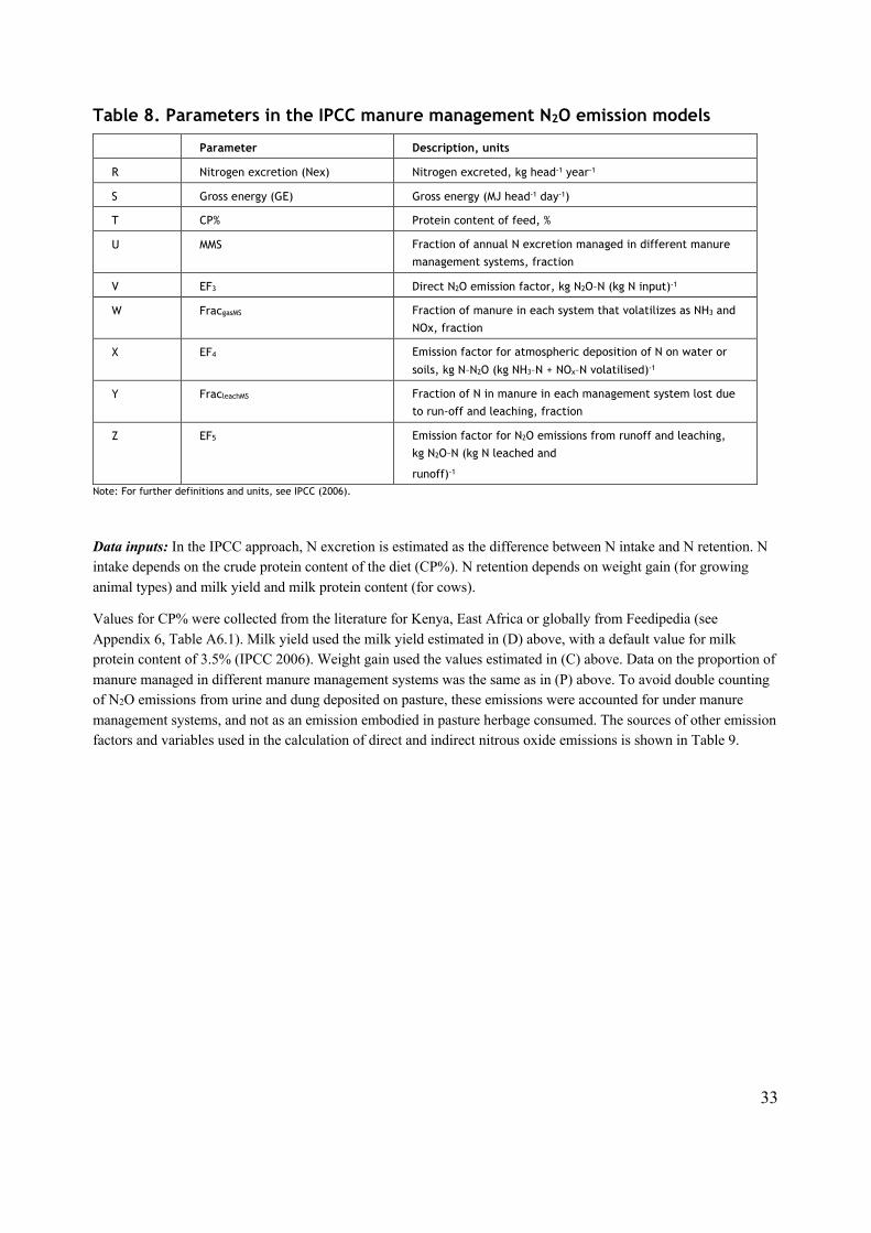
Table 8. Parameters in the IPCC manure management N2O emission models


R Nitrogen excretion (Nex) Nitrogen excreted, kg head-1 year-1

S Gross energy (GE) Gross energy (MJ head-1 day-1)

T CP% Protein content of feed, %

U MMS Fraction of annual N excretion managed in different manure

management systems, fraction

V EF3 Direct N2O emission factor, kg N2O–N (kg N input)-1

W FracgasMS Fraction of manure in each system that volatilizes as NH3 and

NOx, fraction

X EF4 Emission factor for atmospheric deposition of N on water or

soils, kg N–N2O (kg NH3–N + NOx–N volatilised)-1

Y FracleachMS Fraction of N in manure in each management system lost due

to run-off and leaching, fraction

Z EF5 Emission factor for N2O emissions from runoff and leaching,

kg N2O–N (kg N leached and

runoff)-1 Note: For further definitions and units, see IPCC (2006).

Data inputs: In the IPCC approach, N excretion is estimated as the difference between N intake and N retention. N intake depends on the crude protein content of the diet (CP%). N retention depends on weight gain (for growing animal types) and milk yield and milk protein content (for cows).

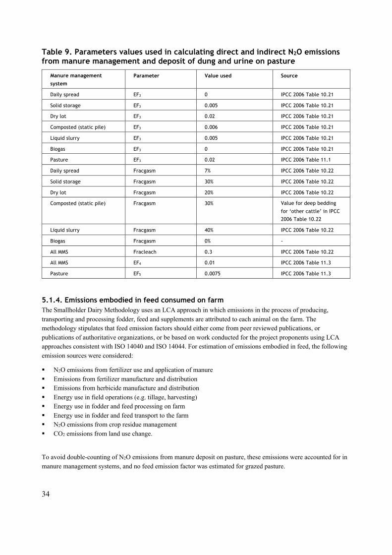
Values for CP% were collected from the literature for Kenya, East Africa or globally from Feedipedia (see Appendix 6, Table A6.1). Milk yield used the milk yield estimated in (D) above, with a default value for milk protein content of 3.5% (IPCC 2006). Weight gain used the values estimated in (C) above. Data on the proportion of manure managed in different manure management systems was the same as in (P) above. To avoid double counting of N2O emissions from urine and dung deposited on pasture, these emissions were accounted for under manure management systems, and not as an emission embodied in pasture herbage consumed. The sources of other emission factors and variables used in the calculation of direct and indirect nitrous oxide emissions is shown in Table 9.

34

Table 9. Parameters values used in calculating direct and indirect N2O emissions from manure management and deposit of dung and urine on pasture

Manure management system

Parameter Value used Source

Daily spread EF3 0 IPCC 2006 Table 10.21

Solid storage EF3 0.005 IPCC 2006 Table 10.21

Dry lot EF3 0.02 IPCC 2006 Table 10.21

Composted (static pile) EF3 0.006 IPCC 2006 Table 10.21

Liquid slurry EF3 0.005 IPCC 2006 Table 10.21

Biogas EF3 0 IPCC 2006 Table 10.21

Pasture EF3 0.02 IPCC 2006 Table 11.1

Daily spread Fracgasm 7% IPCC 2006 Table 10.22

Solid storage Fracgasm 30% IPCC 2006 Table 10.22

Dry lot Fracgasm 20% IPCC 2006 Table 10.22

Composted (static pile) Fracgasm 30% Value for deep bedding

for ‘other cattle’ in IPCC

2006 Table 10.22

Liquid slurry Fracgasm 40% IPCC 2006 Table 10.22

Biogas Fracgasm 0% -

All MMS Fracleach 0.3 IPCC 2006 Table 10.22

All MMS EF4 0.01 IPCC 2006 Table 11.3

Pasture EF5 0.0075 IPCC 2006 Table 11.3

5.1.4. Emissions embodied in feed consumed on farm The Smallholder Dairy Methodology uses an LCA approach in which emissions in the process of producing, transporting and processing fodder, feed and supplements are attributed to each animal on the farm. The methodology stipulates that feed emission factors should either come from peer reviewed publications, or publications of authoritative organizations, or be based on work conducted for the project proponents using LCA approaches consistent with ISO 14040 and ISO 14044. For estimation of emissions embodied in feed, the following emission sources were considered:

§ N2O emissions from fertilizer use and application of manure § Emissions from fertilizer manufacture and distribution § Emissions from herbicide manufacture and distribution § Energy use in field operations (e.g. tillage, harvesting) § Energy use in fodder and feed processing on farm § Energy use in fodder and feed transport to the farm § N2O emissions from crop residue management § CO2 emissions from land use change.

To avoid double-counting of N2O emissions from manure deposit on pasture, these emissions were accounted for in manure management systems, and no feed emission factor was estimated for grazed pasture.

35

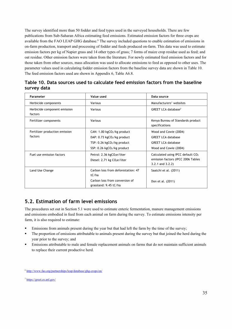
The survey identified more than 50 fodder and feed types used in the surveyed households. There are few publications from Sub-Saharan Africa estimating feed emissions. Estimated emission factors for three crops are available from the FAO LEAP GHG database.6 The survey included questions to enable estimation of emissions in on-farm production, transport and processing of fodder and feeds produced on-farm. This data was used to estimate emission factors per kg of Napier grass and 14 other types of grass; 7 forms of maize crop residue used as feed; and oat residue. Other emission factors were taken from the literature. For newly estimated feed emission factors and for those taken from other sources, mass allocation was used to allocate emissions to feed as opposed to other uses. The parameter values used in calculating fodder emission factors from the baseline survey data are shown in Table 10. The feed emission factors used are shown in Appendix 6, Table A6.8.

Table 10. Data sources used to calculate feed emission factors from the baseline survey data

Parameter Value used Data source

Herbicide components Various Manufacturers’ websites

Herbicide component emission

factors

Various GREET LCA database7

Fertilizer components Various Kenya Bureau of Standards product

specifications

Fertilizer production emission

factors CAN: 1.00 kgCO2/kg product

DAP: 0.73 kgCO2/kg product

TSP: 0.26 kgCO2/kg product

SSP: 0.26 kgCO2/kg product

Wood and Cowie (2004)

GREET LCA database

GREET LCA database

Wood and Cowie (2004)

Fuel use emission factors Petrol: 2.36 kgCO2e/liter

Diesel: 2.71 kg CO2e/liter

Calculated using IPCC default CO2

emission factors (IPCC 2006 Tables

3.2.1 and 3.2.2)

Land Use Change Carbon loss from deforestation: 47

tC/ha

Carbon loss from conversion of

grassland: 9.45 tC/ha

Saatchi et al. (2011)

Don et al. (2011)

5.2. Estimation of farm level emissions The procedures set out in Section 5.1 were used to estimate enteric fermentation, manure management emissions and emissions embodied in feed from each animal on farm during the survey. To estimate emissions intensity per farm, it is also required to estimate:

§ Emissions from animals present during the year but that had left the farm by the time of the survey; § The proportion of emissions attributable to animals present during the survey but that joined the herd during the

year prior to the survey; and § Emissions attributable to male and female replacement animals on farms that do not maintain sufficient animals

to replace their current productive herd.

6 http://www.fao.org/partnerships/leap/database/ghg-crops/en/

7 https://greet.es.anl.gov/

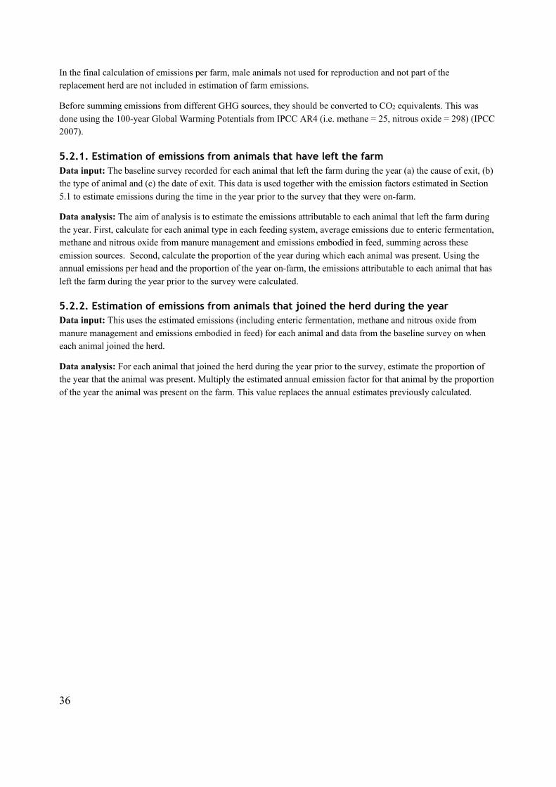
36

In the final calculation of emissions per farm, male animals not used for reproduction and not part of the replacement herd are not included in estimation of farm emissions.

Before summing emissions from different GHG sources, they should be converted to CO2 equivalents. This was done using the 100-year Global Warming Potentials from IPCC AR4 (i.e. methane = 25, nitrous oxide = 298) (IPCC 2007).

5.2.1. Estimation of emissions from animals that have left the farm Data input: The baseline survey recorded for each animal that left the farm during the year (a) the cause of exit, (b) the type of animal and (c) the date of exit. This data is used together with the emission factors estimated in Section 5.1 to estimate emissions during the time in the year prior to the survey that they were on-farm.

Data analysis: The aim of analysis is to estimate the emissions attributable to each animal that left the farm during the year. First, calculate for each animal type in each feeding system, average emissions due to enteric fermentation, methane and nitrous oxide from manure management and emissions embodied in feed, summing across these emission sources. Second, calculate the proportion of the year during which each animal was present. Using the annual emissions per head and the proportion of the year on-farm, the emissions attributable to each animal that has left the farm during the year prior to the survey were calculated.

5.2.2. Estimation of emissions from animals that joined the herd during the year Data input: This uses the estimated emissions (including enteric fermentation, methane and nitrous oxide from manure management and emissions embodied in feed) for each animal and data from the baseline survey on when each animal joined the herd.

Data analysis: For each animal that joined the herd during the year prior to the survey, estimate the proportion of the year that the animal was present. Multiply the estimated annual emission factor for that animal by the proportion of the year the animal was present on the farm. This value replaces the annual estimates previously calculated.

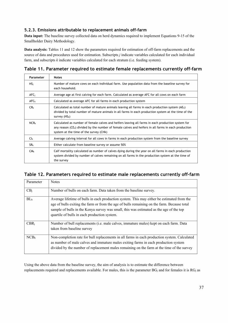
37

5.2.3. Emissions attributable to replacement animals off-farm Data input: The baseline survey collected data on herd dynamics required to implement Equations 9-15 of the Smallholder Dairy Methodology.

Data analysis: Tables 11 and 12 show the parameters required for estimation of off-farm replacements and the source of data and procedures used for estimation. Subscripts j indicate variables calculated for each individual farm, and subscripts k indicate variables calculated for each stratum (i.e. feeding system).

Table 11. Parameter required to estimate female replacements currently off-farm

Parameter Notes

HSj Number of mature cows on each individual farm. Use population data from the baseline survey for

each household.

AFCj Average age at first calving for each farm. Calculated as average AFC for all cows on each farm

AFCk Calculated as average AFC for all farms in each production system

CRk Calculated as total number of mature animals leaving all farms in each production system (AEk)

divided by total number of mature animals in all farms in each production system at the time of the

survey (HSk)

NCRk Calculated as number of female calves and heifers leaving all farms in each production system for

any reason (CEk) divided by the number of female calves and heifers in all farms in each production

system at the time of the survey (CHk)

CIk Average calving interval for all cows in farms in each production system from the baseline survey

SRk Either calculate from baseline survey or assume 50%

CMk Calf mortality calculated as number of calves dying during the year on all farms in each production

system divided by number of calves remaining on all farms in the production system at the time of

the survey

Table 12. Parameters required to estimate male replacements currently off-farm Parameter Notes

CBj Number of bulls on each farm. Data taken from the baseline survey.

BLk Average lifetime of bulls in each production system. This may either be estimated from the age of bulls exiting the farm or from the age of bulls remaining on the farm. Because total sample of bulls in the Kenya survey was small, this was estimated as the age of the top quartile of bulls in each production system.

CBRj Number of bull replacements (i.e. male calves, immature males) kept on each farm. Data taken from baseline survey

NCBk Non-completion rate for bull replacements in all farms in each production system. Calculated as number of male calves and immature males exiting farms in each production system divided by the number of replacement males remaining on the farm at the time of the survey

Using the above data from the baseline survey, the aim of analysis is to estimate the difference between replacements required and replacements available. For males, this is the parameter BGj and for females it is RGj as

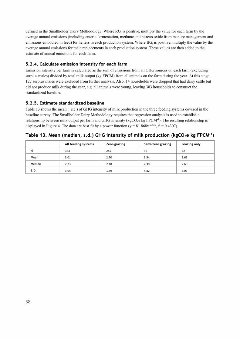
38

defined in the Smallholder Dairy Methodology. Where RGj is positive, multiply the value for each farm by the average annual emissions (including enteric fermentation, methane and nitrous oxide from manure management and emissions embodied in feed) for heifers in each production system. Where BGj is positive, multiply the value by the average annual emissions for male replacements in each production system. These values are then added to the estimate of annual emissions for each farm.

5.2.4. Calculate emission intensity for each farm Emission intensity per farm is calculated as the sum of emissions from all GHG sources on each farm (excluding surplus males) divided by total milk output (kg FPCM) from all animals on the farm during the year. At this stage, 127 surplus males were excluded from further analysis. Also, 14 households were dropped that had dairy cattle but did not produce milk during the year, e.g. all animals were young, leaving 383 households to construct the standardized baseline.

5.2.5. Estimate standardized baseline Table 13 shows the mean (±s.e.) of GHG intensity of milk production in the three feeding systems covered in the baseline survey. The Smallholder Dairy Methodology requires that regression analysis is used to establish a relationship between milk output per farm and GHG intensity (kgCO2e kg FPCM-1). The resulting relationship is displayed in Figure 4. The data are best fit by a power function (y = 81.868x-0.436, r² = 0.4307).

Table 13. Mean (median, s.d.) GHG intensity of milk production (kgCO2e kg FPCM-1)

All feeding systems Zero-grazing Semi-zero grazing Grazing only

N 383 245 96 42

Mean 3.01 2.70 3.54 3.65

Median 2.23 2.18 2.39 2.60

S.D. 3.04 1.89 4.82 3.06

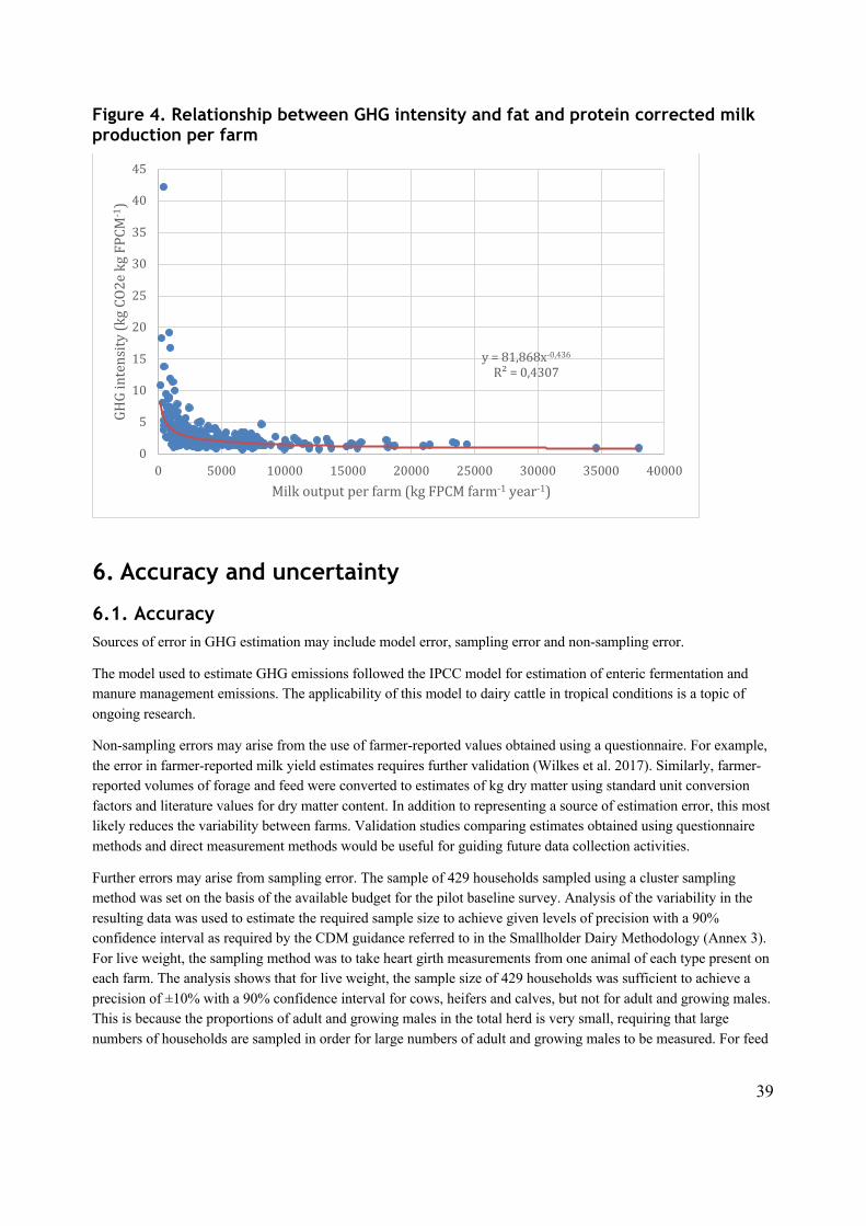
39

Figure 4. Relationship between GHG intensity and fat and protein corrected milk production per farm

6. Accuracy and uncertainty

6.1. Accuracy Sources of error in GHG estimation may include model error, sampling error and non-sampling error.

The model used to estimate GHG emissions followed the IPCC model for estimation of enteric fermentation and manure management emissions. The applicability of this model to dairy cattle in tropical conditions is a topic of ongoing research.

Non-sampling errors may arise from the use of farmer-reported values obtained using a questionnaire. For example, the error in farmer-reported milk yield estimates requires further validation (Wilkes et al. 2017). Similarly, farmer-reported volumes of forage and feed were converted to estimates of kg dry matter using standard unit conversion factors and literature values for dry matter content. In addition to representing a source of estimation error, this most likely reduces the variability between farms. Validation studies comparing estimates obtained using questionnaire methods and direct measurement methods would be useful for guiding future data collection activities.

Further errors may arise from sampling error. The sample of 429 households sampled using a cluster sampling method was set on the basis of the available budget for the pilot baseline survey. Analysis of the variability in the resulting data was used to estimate the required sample size to achieve given levels of precision with a 90% confidence interval as required by the CDM guidance referred to in the Smallholder Dairy Methodology (Annex 3). For live weight, the sampling method was to take heart girth measurements from one animal of each type present on each farm. The analysis shows that for live weight, the sample size of 429 households was sufficient to achieve a precision of ±10% with a 90% confidence interval for cows, heifers and calves, but not for adult and growing males. This is because the proportions of adult and growing males in the total herd is very small, requiring that large numbers of households are sampled in order for large numbers of adult and growing males to be measured. For feed

y=81,868x-0,436

R²=0,4307

0

5

10

15

20

25

30

35

40

45

0 5000 10000 15000 20000 25000 30000 35000 40000

GHGintensity(kgCO2ekgFPCM

-1)

Milkoutputperfarm(kgFPCMfarm-1 year-1)

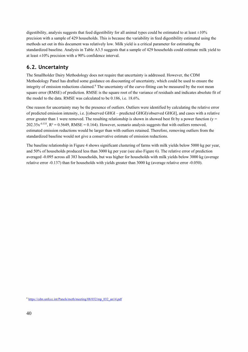
40

digestibility, analysis suggests that feed digestibility for all animal types could be estimated to at least ±10% precision with a sample of 429 households. This is because the variability in feed digestibility estimated using the methods set out in this document was relatively low. Milk yield is a critical parameter for estimating the standardized baseline. Analysis in Table A3.5 suggests that a sample of 429 households could estimate milk yield to at least ±10% precision with a 90% confidence interval.

6.2. Uncertainty The Smallholder Dairy Methodology does not require that uncertainty is addressed. However, the CDM Methodology Panel has drafted some guidance on discounting of uncertainty, which could be used to ensure the integrity of emission reductions claimed.8 The uncertainty of the curve-fitting can be measured by the root mean square error (RMSE) of prediction. RMSE is the square root of the variance of residuals and indicates absolute fit of the model to the data. RMSE was calculated to be 0.186, i.e. 18.6%.

One reason for uncertainty may be the presence of outliers. Outliers were identified by calculating the relative error of predicted emission intensity, i.e. [(observed GHGI – predicted GHGI)/observed GHGI], and cases with a relative error greater than 1 were removed. The resulting relationship is shown in showed best fit by a power function (y = 202.35x-0.535, R² = 0.5649, RMSE = 0.164). However, scenario analysis suggests that with outliers removed, estimated emission reductions would be larger than with outliers retained. Therefore, removing outliers from the standardized baseline would not give a conservative estimate of emission reductions.

The baseline relationship in Figure 4 shows significant clustering of farms with milk yields below 5000 kg per year, and 50% of households produced less than 3000 kg per year (see also Figure 6). The relative error of prediction averaged -0.095 across all 383 households, but was higher for households with milk yields below 3000 kg (average relative error -0.137) than for households with yields greater than 3000 kg (average relative error -0.050).

8 https://cdm.unfccc.int/Panels/meth/meeting/08/032/mp_032_an14.pdf

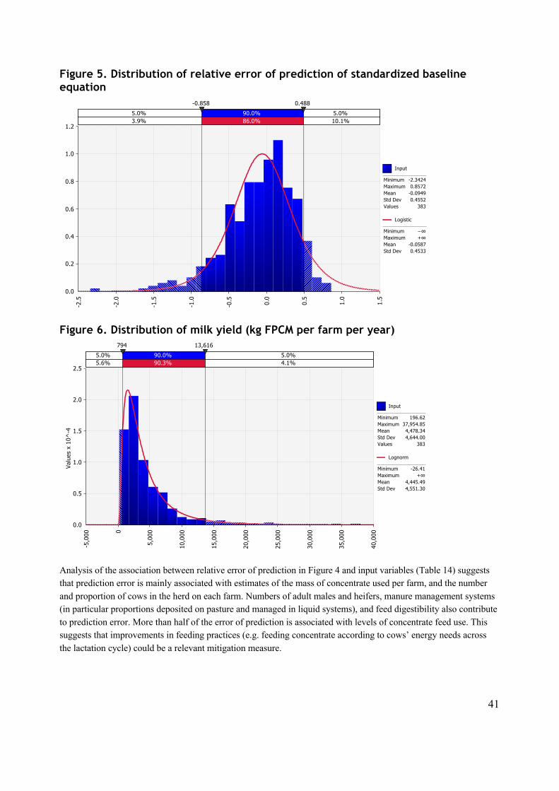
41

Figure 5. Distribution of relative error of prediction of standardized baseline equation

Figure 6. Distribution of milk yield (kg FPCM per farm per year)

Analysis of the association between relative error of prediction in Figure 4 and input variables (Table 14) suggests that prediction error is mainly associated with estimates of the mass of concentrate used per farm, and the number and proportion of cows in the herd on each farm. Numbers of adult males and heifers, manure management systems (in particular proportions deposited on pasture and managed in liquid systems), and feed digestibility also contribute to prediction error. More than half of the error of prediction is associated with levels of concentrate feed use. This suggests that improvements in feeding practices (e.g. feeding concentrate according to cows’ energy needs across the lactation cycle) could be a relevant mitigation measure.

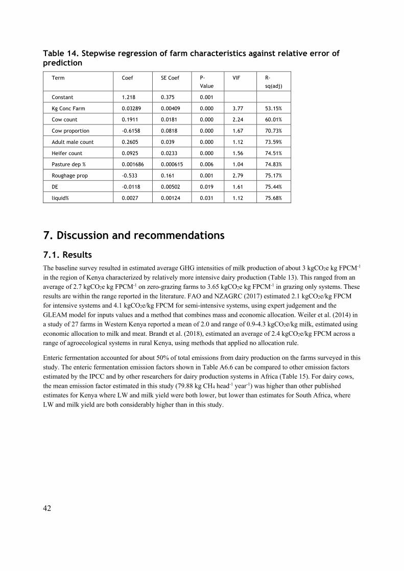
42

Table 14. Stepwise regression of farm characteristics against relative error of prediction

Term Coef SE Coef P-

Value

VIF R-

sq(adj)

Constant 1.218 0.375 0.001

Kg Conc Farm 0.03289 0.00409 0.000 3.77 53.15%

Cow count 0.1911 0.0181 0.000 2.24 60.01%

Cow proportion -0.6158 0.0818 0.000 1.67 70.73%

Adult male count 0.2605 0.039 0.000 1.12 73.59%

Heifer count 0.0925 0.0233 0.000 1.56 74.51%

Pasture dep % 0.001686 0.000615 0.006 1.04 74.83%

Roughage prop -0.533 0.161 0.001 2.79 75.17%

DE -0.0118 0.00502 0.019 1.61 75.44%

liquid% 0.0027 0.00124 0.031 1.12 75.68%

7. Discussion and recommendations

7.1. Results The baseline survey resulted in estimated average GHG intensities of milk production of about 3 kgCO2e kg FPCM-1 in the region of Kenya characterized by relatively more intensive dairy production (Table 13). This ranged from an average of 2.7 kgCO2e kg FPCM-1 on zero-grazing farms to 3.65 kgCO2e kg FPCM-1 in grazing only systems. These results are within the range reported in the literature. FAO and NZAGRC (2017) estimated 2.1 kgCO2e/kg FPCM for intensive systems and 4.1 kgCO2e/kg FPCM for semi-intensive systems, using expert judgement and the GLEAM model for inputs values and a method that combines mass and economic allocation. Weiler et al. (2014) in a study of 27 farms in Western Kenya reported a mean of 2.0 and range of 0.9-4.3 kgCO2e/kg milk, estimated using economic allocation to milk and meat. Brandt et al. (2018), estimated an average of 2.4 kgCO2e/kg FPCM across a range of agroecological systems in rural Kenya, using methods that applied no allocation rule.

Enteric fermentation accounted for about 50% of total emissions from dairy production on the farms surveyed in this study. The enteric fermentation emission factors shown in Table A6.6 can be compared to other emission factors estimated by the IPCC and by other researchers for dairy production systems in Africa (Table 15). For dairy cows, the mean emission factor estimated in this study (79.88 kg CH4 head-1 year-1) was higher than other published estimates for Kenya where LW and milk yield were both lower, but lower than estimates for South Africa, where LW and milk yield are both considerably higher than in this study.

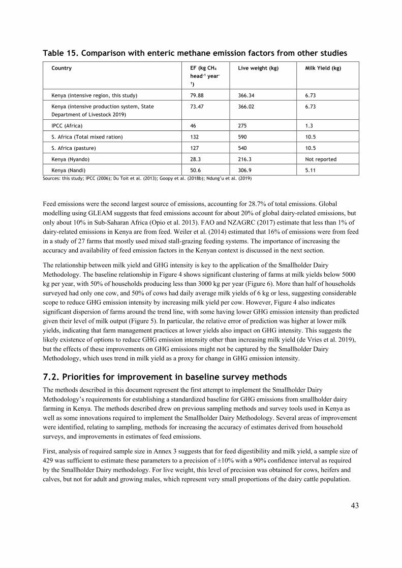
43

Table 15. Comparison with enteric methane emission factors from other studies

Country EF (kg CH4 head-1 year-

1)

Live weight (kg) Milk Yield (kg)

Kenya (intensive region, this study) 79.88 366.34 6.73

Kenya (intensive production system, State

Department of Livestock 2019) 73.47 366.02 6.73

IPCC (Africa) 46 275 1.3

S. Africa (Total mixed ration) 132 590 10.5

S. Africa (pasture) 127 540 10.5

Kenya (Nyando) 28.3 216.3 Not reported

Kenya (Nandi) 50.6 306.9 5.11 Sources: this study; IPCC (2006); Du Toit et al. (2013); Goopy et al. (2018b); Ndung’u et al. (2019)

Feed emissions were the second largest source of emissions, accounting for 28.7% of total emissions. Global modelling using GLEAM suggests that feed emissions account for about 20% of global dairy-related emissions, but only about 10% in Sub-Saharan Africa (Opio et al. 2013). FAO and NZAGRC (2017) estimate that less than 1% of dairy-related emissions in Kenya are from feed. Weiler et al. (2014) estimated that 16% of emissions were from feed in a study of 27 farms that mostly used mixed stall-grazing feeding systems. The importance of increasing the accuracy and availability of feed emission factors in the Kenyan context is discussed in the next section.

The relationship between milk yield and GHG intensity is key to the application of the Smallholder Dairy Methodology. The baseline relationship in Figure 4 shows significant clustering of farms at milk yields below 5000 kg per year, with 50% of households producing less than 3000 kg per year (Figure 6). More than half of households surveyed had only one cow, and 50% of cows had daily average milk yields of 6 kg or less, suggesting considerable scope to reduce GHG emission intensity by increasing milk yield per cow. However, Figure 4 also indicates significant dispersion of farms around the trend line, with some having lower GHG emission intensity than predicted given their level of milk output (Figure 5). In particular, the relative error of prediction was higher at lower milk yields, indicating that farm management practices at lower yields also impact on GHG intensity. This suggests the likely existence of options to reduce GHG emission intensity other than increasing milk yield (de Vries et al. 2019), but the effects of these improvements on GHG emissions might not be captured by the Smallholder Dairy Methodology, which uses trend in milk yield as a proxy for change in GHG emission intensity.

7.2. Priorities for improvement in baseline survey methods The methods described in this document represent the first attempt to implement the Smallholder Dairy Methodology’s requirements for establishing a standardized baseline for GHG emissions from smallholder dairy farming in Kenya. The methods described drew on previous sampling methods and survey tools used in Kenya as well as some innovations required to implement the Smallholder Dairy Methodology. Several areas of improvement were identified, relating to sampling, methods for increasing the accuracy of estimates derived from household surveys, and improvements in estimates of feed emissions.

First, analysis of required sample size in Annex 3 suggests that for feed digestibility and milk yield, a sample size of 429 was sufficient to estimate these parameters to a precision of ±10% with a 90% confidence interval as required by the Smallholder Dairy methodology. For live weight, this level of precision was obtained for cows, heifers and calves, but not for adult and growing males, which represent very small proportions of the dairy cattle population.

44

For weight gain of growing animal types (e.g. heifers, calves), the one-off survey method used here was not able to accurately measure animal growth (i.e. change in weight over time). The live weight data collected were analysed to estimate typical growth curves for male and female growing cattle, which were used to estimate average weight gain for each animal sub-category. The effects of this method would be to reduce the variability in weight gain achieved by animals on different farms.

Second, the methods described here did not account for consumption of milk by calves. While the survey tool did indicate whether the age at weaning of each calf on surveyed farms, no further details on feeding methods were collected. Since bucket feeding is common, the survey tool was therefore not able to distinguish between farmer-reported milk yields that did and did not account for calf consumption of milk. Future surveys should further elaborate questions to determine this.

Third, previous analysis of the uncertainty associated with enteric fermentation emissions from dairy cattle in Kenya estimated using the IPCC Tier 2 model (State Department of Livestock 2019) highlighted that the main variables contributing to uncertainty of emission factor estimates were the methane conversion factor (Ym), feed digestibility, live weight and weight gain, especially for cows and heifers that make up 73% of the animals enumerated in the baseline survey. In the absence of country-specific research, the IPCC default factor for Ym was used. Feed digestibility estimates were based on a combination of feed composition data from the survey and literature values for feed chemical composition. The baseline survey tool collects farmer reported data on feeds fed to different animal types in different seasons. Analyzing the data collected, for roughage, out of 1862 reports of roughages fed by 397 households, 70% were reported as being fed to all dairy cattle, and 30% were fed to particular sub-categories of cattle. Of 669 reports of concentrates and other feed fed, 40% were fed to all dairy cattle and 60% were fed to particular sub-categories, most often (80% of cases) cows. These figures suggest that in the intensive dairy farming region of Kenya, survey tools that aim to identify feed composition for particular animal sub-categories should be able to more accurately reflect diets than methods that estimate available feed only, particularly for cows. The error associated with farmer estimates of volumes fed and their conversion to kg dry matter is unknown. Refusals of feed fed is known to occur (e.g. Methu et al. 2001), but were not accounted for using the methods applied here. While the overall estimates of feed digestibility for each cattle sub-category (Table A6.5) are close to the IPCC default value for dairy cattle in Africa, and are broadly consistent with other literature reports (e.g. Goopy et al. 2018b, Ndung’u et al. 2019), improvements in methods for feed composition data collection and feed chemical composition measurements should be a future priority.

In addition to the sources of uncertainty identified in previous research, the standardized baseline is likely to be sensitive to milk yield estimates, as milk yield appears in both the dependent and independent variable used to estimate the milk yield–GHG intensity relationship. Milk yield estimates were based on farmer-reported milk yields and estimates of the number of days in lactation. Some previous research has indicated that farmer-reported milk yield estimates can be quite accurate in low-yield production systems (Zezza et al. 2016), but sources of error in higher yield systems such as Kenya are not known, and factors such as extended lactations, calf suckling practices, and gendered ownership of morning and evening milk may influence the accuracy of farmer-reported milk yield estimates (Wilkes et al. 2018). Further research is required to validate the accuracy of farmer self-reported milk yields and different methods for estimating annual milk yields using recall methods.

Feed emissions also accounted for a significant proportion of total emissions. To date, there are few estimates of feed emission factors for Sub-Saharan Africa. The baseline survey collected data to enable estimation of emission factors for some key forage components, such as Napier and maize. However, missing data was common for feed production data and, as with milk yield, crop yield data estimated using farmer self-reported estimates may not be accurate, particularly for fodder crops that are harvested multiple times through the year. For concentrates and purchased feeds, the emissions embodied in many ingredients were estimated using emission factors from

45

FEEDPRINT, a database of emission factors developed for the Dutch livestock sector.9 It can be expected that compared to Dutch feed manufacturers, energy use efficiency would be much lower in Kenya (KMT 2017), and the operating margin grid emission factor for the Netherlands (ca. 0.43 tCO2e/MWh) is lower than for Kenya (ca. 0.66 tCO2e/MWh), but production inputs used and transport distances would vary. It has not been possible to assess the effects on uncertainty of using the FEEDPRINT database as a data source. Further research is required to provide more representative and accurate estimates of the GHG intensity of fodder and feed production, processing and transport in Kenya.

7.3. Cost effectiveness of the methodology The premise of the Smallholder Dairy Methodology is that, since dairy development initiatives will mostly track change in milk yields anyway, by establishing a relationship between milk yield and GHG emission intensity at the regional level, the costs of monitoring GHG emissions due to project interventions is decreased. The cost of data collection and analysis for establishing the regional standardized performance baseline was about US$75,000. Following the Smallholder Dairy Methodology, the baseline remains valid for a crediting period of 7 years. The costs of baseline data collection are therefore much lower than for methodologies that require the collection of the full set of baseline data for each participating farm. The Kenya dairy NAMA targets about 155,000 farms, so the cost of baseline setting for each participating farm would be about US$ 0.1. If smaller dairy mitigation initiatives are implemented in the region covered by a baseline survey, with 30,000 participating farms, the cost of baseline setting is about US$ 0.78 per participating farm.

8. Conclusions This pilot baseline survey, conducted in central Kenya, has demonstrated practical methods for setting a regional standardized performance baseline survey to measure the GHG effects of dairy development initiatives. The pilot has shown that collection and analysis of baseline data in accordance with the requirements of the Smallholder Dairy Methodology is feasible and cost-effective. The data collected through the sampling approach described here was capable of achieving precision of ±10% with a confidence interval of 90% for the key parameters driving GHG emissions for most cattle types. Improvements to the data collection tool and measurement methods can further increase the accuracy of the data used. The results from central Kenya show that the regression of milk yield against GHG intensity has an uncertainty of about 18.6%. The Smallholder Dairy Methodology does not require that uncertainty is quantified, but other dairy development initiatives wishing to quantify GHG emission reductions or mitigation actions targeting the dairy sector can apply the estimated uncertainty to discount emission reductions and ensure that claims are conservative. More generally, setting standardized performance baselines for livestock or crop types may be a cost-effective approach for measuring the GHG effects of mitigation initiatives in other agricultural sub-sectors, which might be more generally applicable to support MRV of agricultural mitigation actions in developing countries.

9 http://webapplicaties.wur.nl/software/feedprintNL/index.asp

46

Appendix

Appendix 1. Baseline data collection tool Note: The actual data collection tool also collected data on management practices, gender roles and financing of farm dairy enterprises. Only the GHG-relevant contents are shown in this appendix. Enumerator: Each time a household has been selected for interview, go to the household and:

(1) Make a brief introduction:

Good morning/afternoon. My name is ___________. We are working for UNIQUE forestry and land use consultants. Together with the Kenya Dairy Board and State Department of Livestock, we are doing a survey about dairy cows and dairy production. Does your household keep dairy cows? [If No, say “thank you” and get another household from the list. If Yes:] Does it keep more than 20 dairy cows? If more than 20 cows, then this household should not be sampled.

(2) Explain in more detail about the survey:

The survey we are doing will provide information to help the State Department of Livestock and Kenya Dairy Board to design programmes of support to dairy farmers. The survey asks questions about the dairy cows that you keep, how you do feeding and other management on the farm, and the services that you use. Are you the person responsible for looking after cattle? [If No, ask to speak to someone, e.g. household head, spouse or another adult household member, who is responsible for dairy cattle on the farm. If Yes, continue:]

(3) Check if the person is willing to be interviewed:

The survey will take about 1 and a half hours. Can you spare some time to talk now? [If No, try to rearrange for later today. If yes, begin the survey]

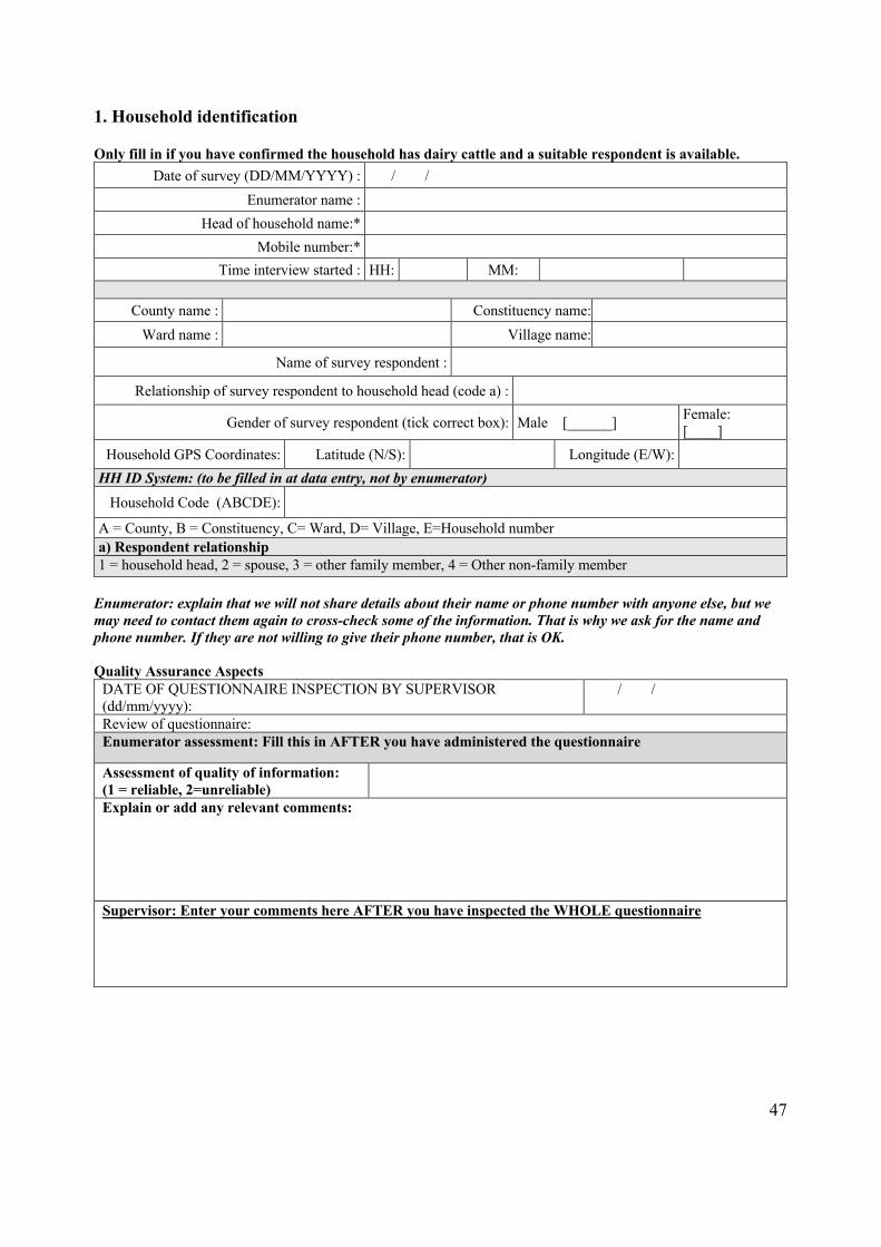
47

1. Household identification Only fill in if you have confirmed the household has dairy cattle and a suitable respondent is available.

Date of survey (DD/MM/YYYY) : / /

Enumerator name :

Head of household name:*

Mobile number:*

Time interview started : HH: MM:

County name : Constituency name:

Ward name : Village name:

Name of survey respondent :

Relationship of survey respondent to household head (code a) :

Gender of survey respondent (tick correct box): Male [______] Female: [____]

Household GPS Coordinates: Latitude (N/S): Longitude (E/W):

HH ID System: (to be filled in at data entry, not by enumerator) Household Code (ABCDE):

A = County, B = Constituency, C= Ward, D= Village, E=Household number a) Respondent relationship 1 = household head, 2 = spouse, 3 = other family member, 4 = Other non-family member

Enumerator: explain that we will not share details about their name or phone number with anyone else, but we may need to contact them again to cross-check some of the information. That is why we ask for the name and phone number. If they are not willing to give their phone number, that is OK. Quality Assurance Aspects

DATE OF QUESTIONNAIRE INSPECTION BY SUPERVISOR (dd/mm/yyyy):

/ /

Review of questionnaire: Enumerator assessment: Fill this in AFTER you have administered the questionnaire

Assessment of quality of information: (1 = reliable, 2=unreliable)

Explain or add any relevant comments: Supervisor: Enter your comments here AFTER you have inspected the WHOLE questionnaire

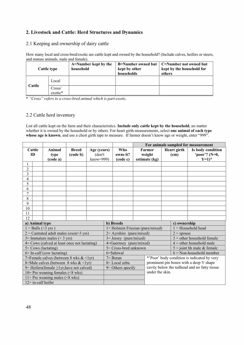
48

2. Livestock and Cattle: Herd Structures and Dynamics 2.1 Keeping and ownership of dairy cattle How many local and cross-bred/exotic are cattle kept and owned by the household? (Include calves, heifers or steers, and mature animals, male and female).

Cattle type A=Number kept by the household

B=Number owned but kept by other households

C=Number not owned but kept by the household for others

Cattle Local

Cross/ exotic*

* “Cross” refers to a cross-bred animal which is part-exotic. 2.2 Cattle herd inventory List all cattle kept on the farm and their characteristics. Include only cattle kept by the household, no matter whether it is owned by the household or by others. For heart girth measurements, select one animal of each type whose age is known, and use a chest girth tape to measure. If farmer doesn’t know age or weight, enter “999”. For animals sampled for measurement

Cattle ID

Animal type

(code a)

Breed (code b)

Age (years) (don't

know=999)

Who owns it? (code c)

Farmer weight

estimate (kg)

Heart girth (cm)

Is body condition ‘poor’? (N=0,

Y=1)* 1 2 3 4 5 6 7 8 9 10 11 12 a) Animal type b) Breeds c) ownership 1 = Bulls (>3 yrs ) 1= Holstein Friesian (pure/mixed) 1 = Household head 2 = Castrated adult males (oxen>3 yrs) 2= Ayrshire (pure/mixed) 2 = spouse 3= Immature males (< 3 yrs) 3= Jersey (pure/mixed) 3 = other household female 4= Cows (calved at least once not lactating) 4=Guernsey (pure/mixed) 4 = other household male 5= Cows (lactating) 5= Cross-bred unknown 5 = joint hh male & female 6= In-calf (cow lactating) 6=Sahiwal 6 = Non-household member 7=Female calves (between 8 wks & <1yr) 7= Boran *’Poor’ body condition is indicated by very

prominent pin bones with a deep V shape cavity below the tailhead and no fatty tissue under the skin.

8=Male calves (between 8 wks & <1yr) 8= Local zebu 9= Heifers(female ≥1yr,have not calved) 9= Others specify 10= Pre weaning females (<8 wks) 11= Pre weaning males (<8 wks) 12= in-calf heifer

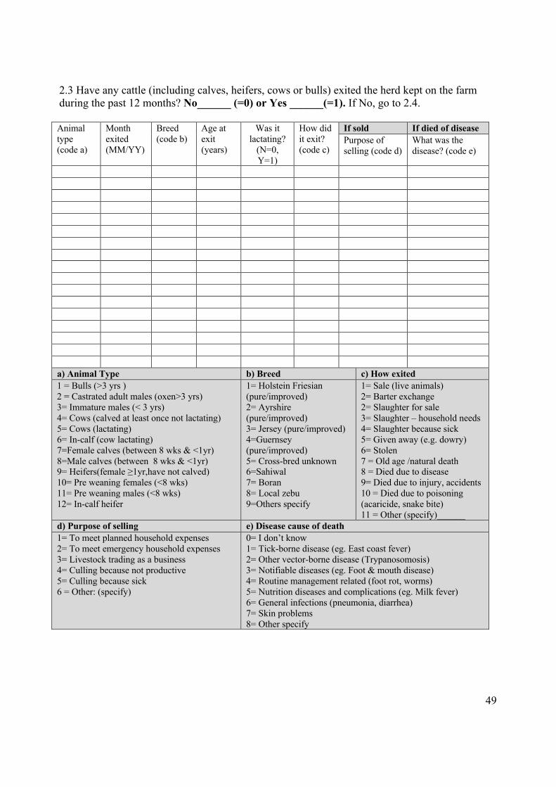
49

2.3 Have any cattle (including calves, heifers, cows or bulls) exited the herd kept on the farm during the past 12 months? No______ (=0) or Yes ______(=1). If No, go to 2.4. Animal type (code a)

Month exited (MM/YY)

Breed (code b)

Age at exit (years)

Was it lactating?

(N=0, Y=1)

How did it exit? (code c)

If sold If died of disease Purpose of selling (code d)

What was the disease? (code e)

a) Animal Type b) Breed c) How exited 1 = Bulls (>3 yrs ) 2 = Castrated adult males (oxen>3 yrs) 3= Immature males (< 3 yrs) 4= Cows (calved at least once not lactating) 5= Cows (lactating) 6= In-calf (cow lactating) 7=Female calves (between 8 wks & <1yr) 8=Male calves (between 8 wks & <1yr) 9= Heifers(female ≥1yr,have not calved) 10= Pre weaning females (<8 wks) 11= Pre weaning males (<8 wks) 12= In-calf heifer

1= Holstein Friesian (pure/improved) 2= Ayrshire (pure/improved) 3= Jersey (pure/improved) 4=Guernsey (pure/improved) 5= Cross-bred unknown 6=Sahiwal 7= Boran 8= Local zebu 9=Others specify

1= Sale (live animals) 2= Barter exchange 2= Slaughter for sale 3= Slaughter – household needs 4= Slaughter because sick 5= Given away (e.g. dowry) 6= Stolen 7 = Old age /natural death 8 = Died due to disease 9= Died due to injury, accidents 10 = Died due to poisoning (acaricide, snake bite) 11 = Other (specify)______

d) Purpose of selling e) Disease cause of death 1= To meet planned household expenses 2= To meet emergency household expenses 3= Livestock trading as a business 4= Culling because not productive 5= Culling because sick 6 = Other: (specify)

0= I don’t know 1= Tick-borne disease (eg. East coast fever) 2= Other vector-borne disease (Trypanosomosis) 3= Notifiable diseases (eg. Foot & mouth disease) 4= Routine management related (foot rot, worms) 5= Nutrition diseases and complications (eg. Milk fever) 6= General infections (pneumonia, diarrhea) 7= Skin problems 8= Other specify

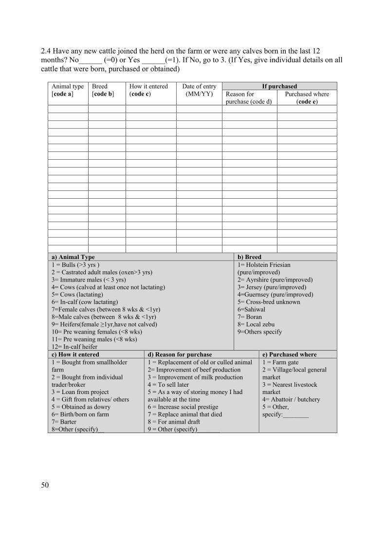
50

2.4 Have any new cattle joined the herd on the farm or were any calves born in the last 12 months? No______ (=0) or Yes ______(=1). If No, go to 3. (If Yes, give individual details on all cattle that were born, purchased or obtained)

Animal type [code a]

Breed [code b]

How it entered (code c)

Date of entry (MM/YY)

If purchased Reason for purchase (code d)

Purchased where (code e)

a) Animal Type b) Breed 1 = Bulls (>3 yrs ) 2 = Castrated adult males (oxen>3 yrs) 3= Immature males (< 3 yrs) 4= Cows (calved at least once not lactating) 5= Cows (lactating) 6= In-calf (cow lactating) 7=Female calves (between 8 wks & <1yr) 8=Male calves (between 8 wks & <1yr) 9= Heifers(female ≥1yr,have not calved) 10= Pre weaning females (<8 wks) 11= Pre weaning males (<8 wks) 12= In-calf heifer

1= Holstein Friesian (pure/improved) 2= Ayrshire (pure/improved) 3= Jersey (pure/improved) 4=Guernsey (pure/improved) 5= Cross-bred unknown 6=Sahiwal 7= Boran 8= Local zebu 9=Others specify

c) How it entered d) Reason for purchase e) Purchased where 1 = Bought from smallholder farm 2 = Bought from individual trader/broker 3 = Loan from project 4 = Gift from relatives/ others 5 = Obtained as dowry 6= Birth/born on farm 7= Barter 8=Other (specify)__

1 = Replacement of old or culled animal 2= Improvement of beef production 3 = Improvement of milk production 4 = To sell later 5 = As a way of storing money I had available at the time 6 = Increase social prestige 7 = Replace animal that died 8 = For animal draft 9 = Other (specify)_______

1 = Farm gate 2 = Village/local general market 3 = Nearest livestock market 4= Abattoir / butchery 5 = Other, specify:________

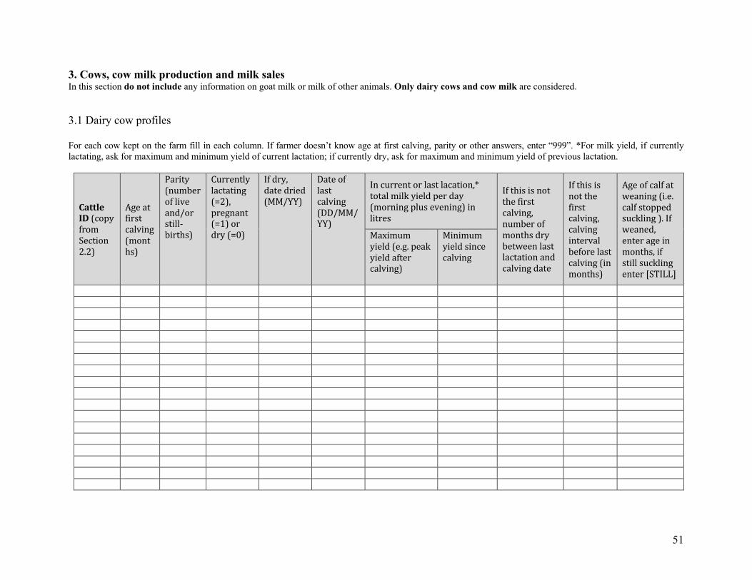
51

3. Cows, cow milk production and milk sales In this section do not include any information on goat milk or milk of other animals. Only dairy cows and cow milk are considered. 3.1 Dairy cow profiles For each cow kept on the farm fill in each column. If farmer doesn’t know age at first calving, parity or other answers, enter “999”. *For milk yield, if currently lactating, ask for maximum and minimum yield of current lactation; if currently dry, ask for maximum and minimum yield of previous lactation.

CattleID(copyfromSection2.2)

Ageatfirstcalving(months)

Parity(numberofliveand/orstill-births)

Currentlylactating(=2),pregnant(=1)ordry(=0)

Ifdry,datedried(MM/YY)

Dateoflastcalving(DD/MM/YY)

Incurrentorlastlacation,*totalmilkyieldperday(morningplusevening)inlitres

Ifthisisnotthefirstcalving,numberofmonthsdrybetweenlastlactationandcalvingdate

Ifthisisnotthefirstcalving,calvingintervalbeforelastcalving(inmonths)

Ageofcalfatweaning(i.e.calfstoppedsuckling).Ifweaned,enterageinmonths,ifstillsucklingenter[STILL]

Maximumyield(e.g.peakyieldaftercalving)

Minimumyieldsincecalving

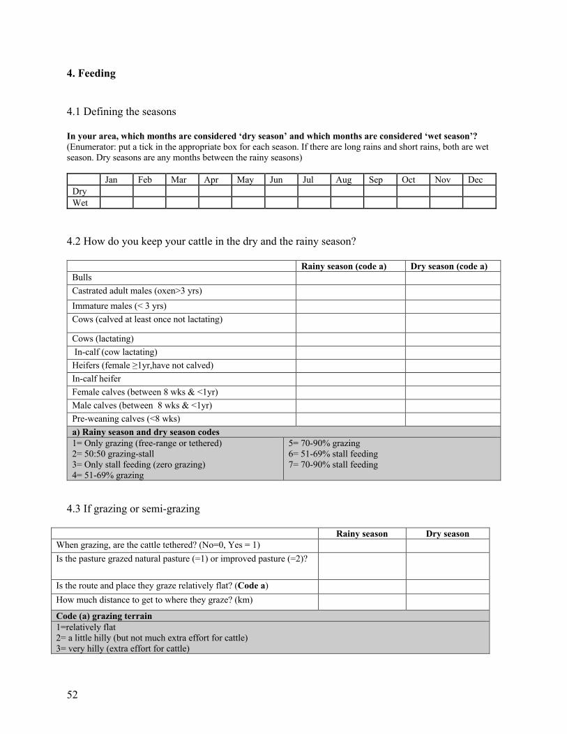
52

4. Feeding 4.1 Defining the seasons In your area, which months are considered ‘dry season’ and which months are considered ‘wet season’? (Enumerator: put a tick in the appropriate box for each season. If there are long rains and short rains, both are wet season. Dry seasons are any months between the rainy seasons)

Jan Feb Mar Apr May Jun Jul Aug Sep Oct Nov Dec Dry Wet

4.2 How do you keep your cattle in the dry and the rainy season?

Rainy season (code a) Dry season (code a) Bulls Castrated adult males (oxen>3 yrs) Immature males (< 3 yrs) Cows (calved at least once not lactating)

Cows (lactating) In-calf (cow lactating) Heifers (female ≥1yr,have not calved) In-calf heifer Female calves (between 8 wks & <1yr)

Male calves (between 8 wks & <1yr) Pre-weaning calves (<8 wks) a) Rainy season and dry season codes 1= Only grazing (free-range or tethered) 2= 50:50 grazing-stall 3= Only stall feeding (zero grazing) 4= 51-69% grazing

5= 70-90% grazing 6= 51-69% stall feeding 7= 70-90% stall feeding

4.3 If grazing or semi-grazing

Rainy season Dry season When grazing, are the cattle tethered? (No=0, Yes = 1) Is the pasture grazed natural pasture (=1) or improved pasture (=2)?

Is the route and place they graze relatively flat? (Code a)

How much distance to get to where they graze? (km)

Code (a) grazing terrain 1=relatively flat 2= a little hilly (but not much extra effort for cattle) 3= very hilly (extra effort for cattle)

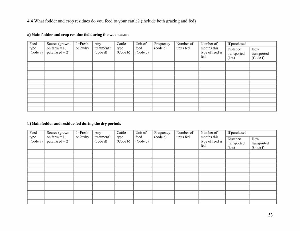
53

4.4 What fodder and crop residues do you feed to your cattle? (include both grazing and fed) a)Mainfodderandcropresiduefedduringthewetseason

Feed

type (Code a)

Source (grown

on farm = 1, purchased = 2)

1=Fresh

or 2=dry

Any

treatment? (code d)

Cattle

type (Code b)

Unit of

feed (Code c)

Frequency

(code e)

Number of

units fed

Number of

months this type of feed is

fed

If purchased:

Distance

transported (km)

How

transported (Code f)

b)Mainfodderandresiduefedduringthedryperiods

Feed

type

(Code a)

Source (grown

on farm = 1,

purchased = 2)

1=Fresh

or 2=dry

Any

treatment?

(code d)

Cattle

type

(Code b)

Unit of

feed

(Code c)

Frequency

(code e)

Number of

units fed

Number of

months this

type of feed is fed

If purchased:

Distance

transported

(km)

How

transported

(Code f)

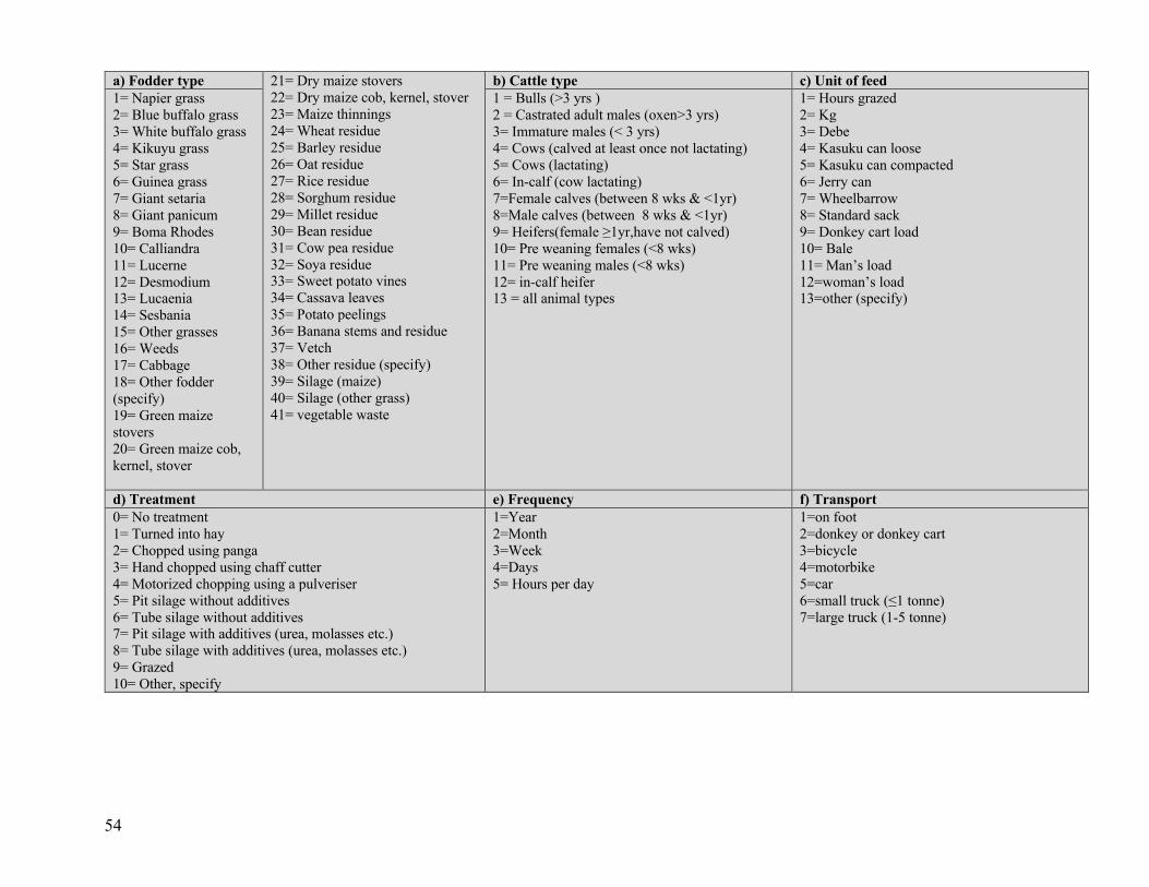
54

a) Fodder type 21= Dry maize stovers

22= Dry maize cob, kernel, stover

23= Maize thinnings

24= Wheat residue

25= Barley residue

26= Oat residue

27= Rice residue

28= Sorghum residue

29= Millet residue

30= Bean residue

31= Cow pea residue

32= Soya residue 33= Sweet potato vines

34= Cassava leaves

35= Potato peelings

36= Banana stems and residue

37= Vetch

38= Other residue (specify)

39= Silage (maize)

40= Silage (other grass)

41= vegetable waste

b) Cattle type c) Unit of feed 1= Napier grass

2= Blue buffalo grass

3= White buffalo grass

4= Kikuyu grass

5= Star grass

6= Guinea grass

7= Giant setaria

8= Giant panicum

9= Boma Rhodes

10= Calliandra

11= Lucerne

12= Desmodium 13= Lucaenia

14= Sesbania

15= Other grasses

16= Weeds

17= Cabbage

18= Other fodder

(specify)

19= Green maize

stovers

20= Green maize cob,

kernel, stover

1 = Bulls (>3 yrs )

2 = Castrated adult males (oxen>3 yrs)

3= Immature males (< 3 yrs)

4= Cows (calved at least once not lactating)

5= Cows (lactating)

6= In-calf (cow lactating)

7=Female calves (between 8 wks & <1yr)

8=Male calves (between 8 wks & <1yr)

9= Heifers(female ≥1yr,have not calved)

10= Pre weaning females (<8 wks)

11= Pre weaning males (<8 wks)

12= in-calf heifer 13 = all animal types

1= Hours grazed

2= Kg

3= Debe

4= Kasuku can loose

5= Kasuku can compacted

6= Jerry can

7= Wheelbarrow

8= Standard sack

9= Donkey cart load

10= Bale

11= Man’s load

12=woman’s load 13=other (specify)

d) Treatment e) Frequency f) Transport 0= No treatment

1= Turned into hay

2= Chopped using panga

3= Hand chopped using chaff cutter

4= Motorized chopping using a pulveriser

5= Pit silage without additives

6= Tube silage without additives 7= Pit silage with additives (urea, molasses etc.)

8= Tube silage with additives (urea, molasses etc.)

9= Grazed

10= Other, specify

1=Year

2=Month

3=Week

4=Days

5= Hours per day

1=on foot

2=donkey or donkey cart

3=bicycle

4=motorbike

5=car

6=small truck (≤1 tonne)

7=large truck (1-5 tonne)

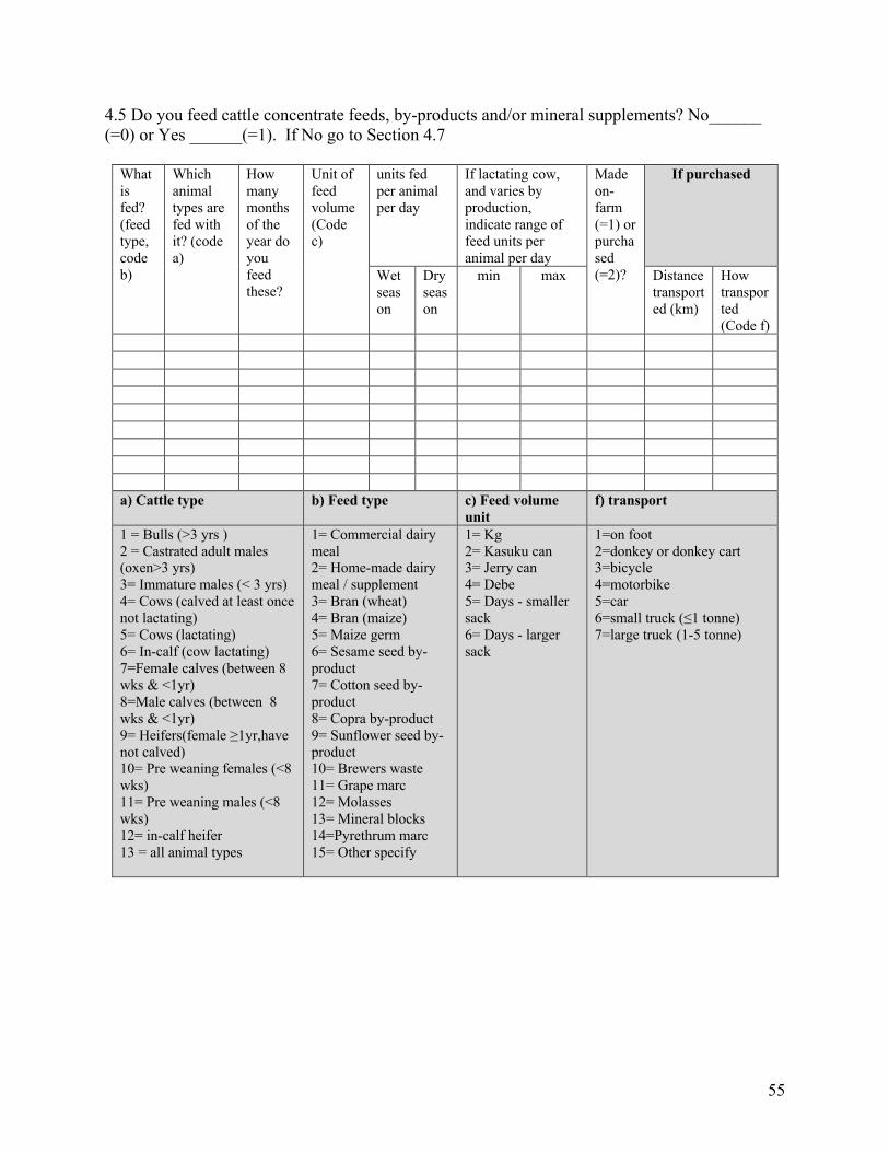
55

4.5 Do you feed cattle concentrate feeds, by-products and/or mineral supplements? No______ (=0) or Yes ______(=1). If No go to Section 4.7

What is fed? (feed type, code b)

Which animal types are fed with it? (code a)

How many months of the year do you feed these?

Unit of feed volume (Code c)

units fed per animal per day

If lactating cow, and varies by production, indicate range of feed units per animal per day

Made on-farm (=1) or purchased (=2)?

If purchased

Wet season

Dry season

min max Distance transported (km)

How transported (Code f)

a) Cattle type b) Feed type c) Feed volume

unit f) transport

1 = Bulls (>3 yrs ) 2 = Castrated adult males (oxen>3 yrs) 3= Immature males (< 3 yrs) 4= Cows (calved at least once not lactating) 5= Cows (lactating) 6= In-calf (cow lactating) 7=Female calves (between 8 wks & <1yr) 8=Male calves (between 8 wks & <1yr) 9= Heifers(female ≥1yr,have not calved) 10= Pre weaning females (<8 wks) 11= Pre weaning males (<8 wks) 12= in-calf heifer 13 = all animal types

1= Commercial dairy meal 2= Home-made dairy meal / supplement 3= Bran (wheat) 4= Bran (maize) 5= Maize germ 6= Sesame seed by-product 7= Cotton seed by-product 8= Copra by-product 9= Sunflower seed by-product 10= Brewers waste 11= Grape marc 12= Molasses 13= Mineral blocks 14=Pyrethrum marc 15= Other specify

1= Kg 2= Kasuku can 3= Jerry can 4= Debe 5= Days - smaller sack 6= Days - larger sack

1=on foot 2=donkey or donkey cart 3=bicycle 4=motorbike 5=car 6=small truck (≤1 tonne) 7=large truck (1-5 tonne)

56

4.6Ifowndairymeal/supplementmadeon-farm,whatdoyouincorporate?

Supplement input (Code a)

Purchased? 1=Yes 0=No

% of mix in dry season % of mix in wet season

a) Dairy meal / supplement input

1= Maize germ 2= Wheat 3= Pollard 4= Molasses 5= Maize bran 6= Wheat bran 7= Soya bean meal

8= Sunflower seed cake 9= Sesbania leaves 10= Calliandra leaves 11= Fish meal 12= Dicalcium Phosphate 13= Limestone

14= Rock phosphate 15= Mineral Premix. 16=Diamond V 17=Kupa Kula 18=Other specify 99=No more supplement

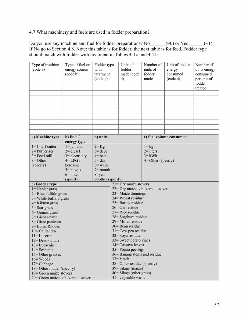
57

4.7 What machinery and fuels are used in fodder preparation? Do you use any machine and fuel for fodder preparations? No______ (=0) or Yes ______(=1). If No go to Section 4.8. Note: this table is for fodder, the next table is for feed. Fodder type should match with fodder with treatment in Tables 4.4.a and 4.4.b.

Type of machine (code a)

Type of fuel or energy source (code b)

Fodder type with treatment (code c)

Units of fodder made (code d)

Number of units of fodder made

Unit of fuel or energy consumed (code d)

Number of units energy consumed per unit of fodder treated

a) Machine type b) Fuel /

energy type d) units e) fuel volume consumed

1= Chaff cutter 2= Pulverizer 3= Feed mill 3= Other (specify)

1=by hand 2= diesel 3= electricity 4= LPG / kerosene 5= biogas 6= other (specify)

2= Kg 3= debe 4= bale 5= day 6= week 7= month 8=year 9=other (specify)

1= kg 2= liters 3= kWh 4= Other (specify)

c) Fodder type 21= Dry maize stovers 22= Dry maize cob, kernel, stover 23= Maize thinnings 24= Wheat residue 25= Barley residue 26= Oat residue 27= Rice residue 28= Sorghum residue 29= Millet residue 30= Bean residue 31= Cow pea residue 32= Soya residue 33= Sweet potato vines 34= Cassava leaves 35= Potato peelings 36= Banana stems and residue 37= Vetch 38= Other residue (specify) 39= Silage (maize) 40= Silage (other grass) 41= vegetable waste

1= Napier grass 2= Blue buffalo grass 3= White buffalo grass 4= Kikuyu grass 5= Star grass 6= Guinea grass 7= Giant setaria 8= Giant panicum 9= Boma Rhodes 10= Calliandra 11= Lucerne 12= Desmodium 13= Lucaenia 14= Sesbania 15= Other grasses 16= Weeds 17= Cabbage 18= Other fodder (specify) 19= Green maize stovers 20= Green maize cob, kernel, stover

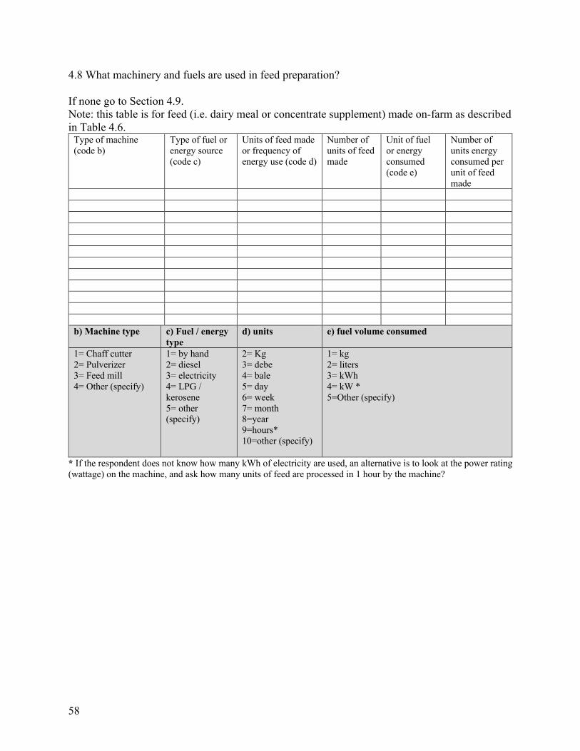
58

4.8 What machinery and fuels are used in feed preparation? If none go to Section 4.9. Note: this table is for feed (i.e. dairy meal or concentrate supplement) made on-farm as described in Table 4.6.

Type of machine (code b)

Type of fuel or energy source (code c)

Units of feed made or frequency of energy use (code d)

Number of units of feed made

Unit of fuel or energy consumed (code e)

Number of units energy consumed per unit of feed made

b) Machine type c) Fuel / energy

type d) units e) fuel volume consumed

1= Chaff cutter 2= Pulverizer 3= Feed mill 4= Other (specify)

1= by hand 2= diesel 3= electricity 4= LPG / kerosene 5= other (specify)

2= Kg 3= debe 4= bale 5= day 6= week 7= month 8=year 9=hours* 10=other (specify)

1= kg 2= liters 3= kWh 4= kW * 5=Other (specify)

* If the respondent does not know how many kWh of electricity are used, an alternative is to look at the power rating (wattage) on the machine, and ask how many units of feed are processed in 1 hour by the machine?

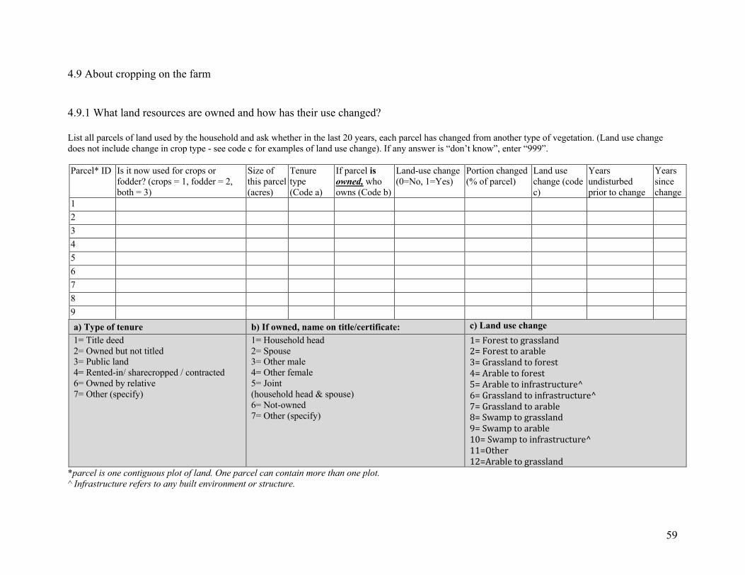
59

4.9 About cropping on the farm 4.9.1 What land resources are owned and how has their use changed? List all parcels of land used by the household and ask whether in the last 20 years, each parcel has changed from another type of vegetation. (Land use change does not include change in crop type - see code c for examples of land use change). If any answer is “don’t know”, enter “999”. Parcel* ID Is it now used for crops or

fodder? (crops = 1, fodder = 2, both = 3)

Size of this parcel (acres)

Tenure type (Code a)

If parcel is owned, who owns (Code b)

Land-use change (0=No, 1=Yes)

Portion changed (% of parcel)

Land use change (code c)

Years undisturbed prior to change

Years since change

1

2

3

4

5

6

7

8

9

a) Type of tenure b) If owned, name on title/certificate: c) Land use change 1= Title deed 2= Owned but not titled 3= Public land 4= Rented-in/ sharecropped / contracted 6= Owned by relative 7= Other (specify)

1= Household head 2= Spouse 3= Other male 4= Other female 5= Joint (household head & spouse) 6= Not-owned 7= Other (specify)

1=Foresttograssland2=Foresttoarable3=Grasslandtoforest4=Arabletoforest5=Arabletoinfrastructure^6=Grasslandtoinfrastructure^7=Grasslandtoarable8=Swamptograssland9=Swamptoarable10=Swamptoinfrastructure^11=Other12=Arabletograssland

*parcel is one contiguous plot of land. One parcel can contain more than one plot. ^ Infrastructure refers to any built environment or structure.

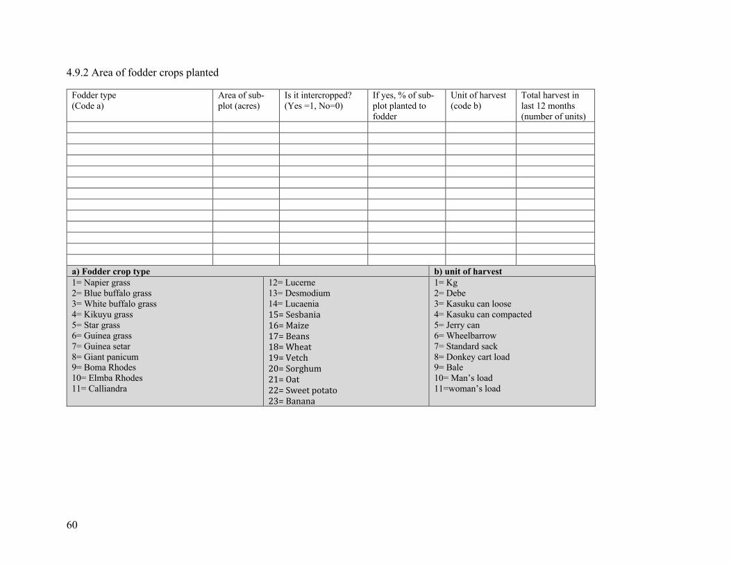
60

4.9.2 Area of fodder crops planted

Fodder type (Code a)

Area of sub-plot (acres)

Is it intercropped? (Yes =1, No=0)

If yes, % of sub-plot planted to fodder

Unit of harvest (code b)

Total harvest in last 12 months (number of units)

a) Fodder crop type b) unit of harvest 1= Napier grass 2= Blue buffalo grass 3= White buffalo grass 4= Kikuyu grass 5= Star grass 6= Guinea grass 7= Guinea setar 8= Giant panicum 9= Boma Rhodes 10= Elmba Rhodes 11= Calliandra

12= Lucerne 13= Desmodium 14= Lucaenia 15=Sesbania 16=Maize 17=Beans 18=Wheat 19=Vetch 20=Sorghum 21=Oat22=Sweetpotato23=Banana

1= Kg 2= Debe 3= Kasuku can loose 4= Kasuku can compacted 5= Jerry can 6= Wheelbarrow 7= Standard sack 8= Donkey cart load 9= Bale 10= Man’s load 11=woman’s load

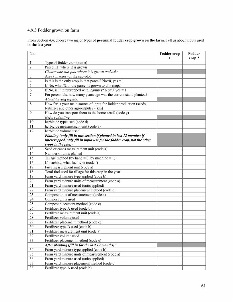
61

4.9.3 Fodder grown on farm From Section 4.4, choose two major types of perennial fodder crop grown on the farm. Tell us about inputs used in the last year.

No. Fodder crop 1

Fodder crop 2

1 Type of fodder crop (name) 2 Parcel ID where it is grown Choose one sub-plot where it is grown and ask: 3 Area (in acres) of the sub-plot 4 Is this is the only crop in that parcel? No=0, yes = 1 5 If No, what % of the parcel is grown to this crop? 6 If No, is it intercropped with legumes? No=0, yes = 1 7 For perennials, how many years ago was the current stand planted? About buying inputs: 8 How far is your main source of input for fodder production (seeds,

fertilizer and other agro-inputs?) (km)

9 How do you transport them to the homestead? (code g) Before planting 10 herbicide type used (code d) 11 herbicide measurement unit (code a) 12 herbicide volume used Planting (only fill in this section if planted in last 12 months; if

intercropped, only fill in input use for the fodder crop, not the other crops in the plot):

13 Seed or canes measurement unit (code a) 14 Number of units planted 15 Tillage method (by hand = 0, by machine = 1) 16 If machine, what fuel type (code f) 17 Fuel measurement unit (code a) 18 Total fuel used for tillage for this crop in the year 19 Farm yard manure type applied (code b) 20 Farm yard manure units of measurement (code a) 21 Farm yard manure used (units applied) 22 Farm yard manure placement method (code c) 23 Compost units of measurement (code a) 24 Compost units used 25 Compost placement method (code c) 26 Fertilizer type A used (code b) 27 Fertilizer measurement unit (code a) 28 Fertilizer volume used 29 Fertilizer placement method (code c) 30 Fertilizer type B used (code b) 31 Fertilizer measurement unit (code a) 32 Fertilizer volume used 33 Fertilizer placement method (code c) After planting (fill in for the last 12 months): 34 Farm yard manure type applied (code b) 35 Farm yard manure units of measurement (code a) 36 Farm yard manure used (units applied) 37 Farm yard manure placement method (code c) 38 Fertilizer type A used (code b)

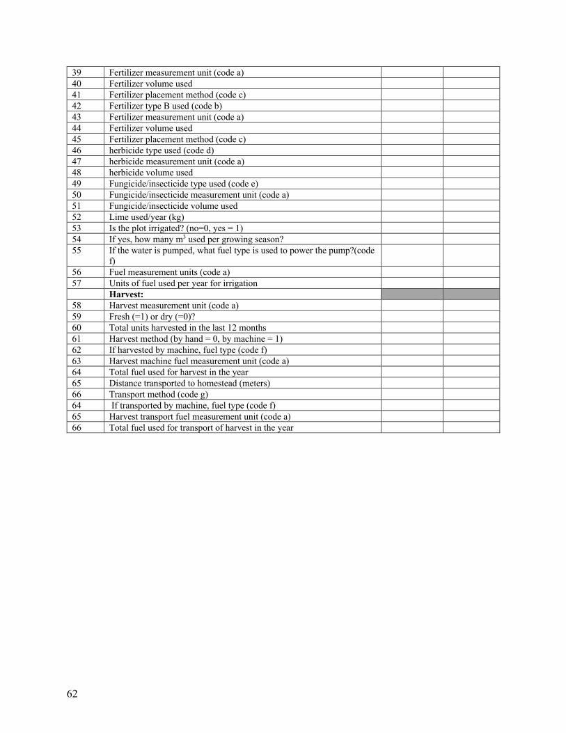
62

39 Fertilizer measurement unit (code a) 40 Fertilizer volume used 41 Fertilizer placement method (code c) 42 Fertilizer type B used (code b) 43 Fertilizer measurement unit (code a) 44 Fertilizer volume used 45 Fertilizer placement method (code c) 46 herbicide type used (code d) 47 herbicide measurement unit (code a) 48 herbicide volume used 49 Fungicide/insecticide type used (code e) 50 Fungicide/insecticide measurement unit (code a) 51 Fungicide/insecticide volume used 52 Lime used/year (kg) 53 Is the plot irrigated? (no=0, yes = 1) 54 If yes, how many m3 used per growing season? 55 If the water is pumped, what fuel type is used to power the pump?(code

f)

56 Fuel measurement units (code a) 57 Units of fuel used per year for irrigation Harvest: 58 Harvest measurement unit (code a) 59 Fresh (=1) or dry (=0)? 60 Total units harvested in the last 12 months 61 Harvest method (by hand = 0, by machine = 1) 62 If harvested by machine, fuel type (code f) 63 Harvest machine fuel measurement unit (code a) 64 Total fuel used for harvest in the year 65 Distance transported to homestead (meters) 66 Transport method (code g) 64 If transported by machine, fuel type (code f) 65 Harvest transport fuel measurement unit (code a) 66 Total fuel used for transport of harvest in the year

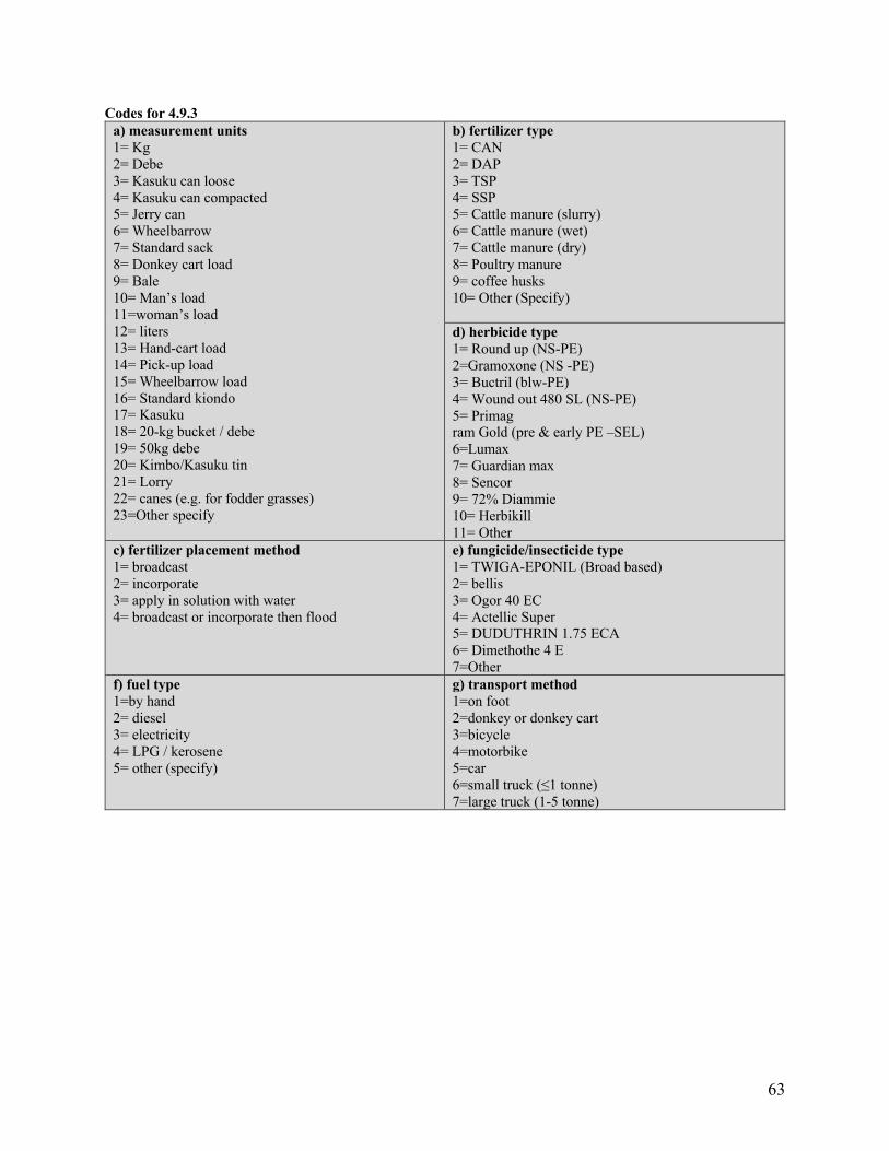
63

Codes for 4.9.3 a) measurement units 1= Kg 2= Debe 3= Kasuku can loose 4= Kasuku can compacted 5= Jerry can 6= Wheelbarrow 7= Standard sack 8= Donkey cart load 9= Bale 10= Man’s load 11=woman’s load 12= liters 13= Hand-cart load 14= Pick-up load 15= Wheelbarrow load 16= Standard kiondo 17= Kasuku 18= 20-kg bucket / debe 19= 50kg debe 20= Kimbo/Kasuku tin 21= Lorry 22= canes (e.g. for fodder grasses) 23=Other specify

b) fertilizer type 1= CAN 2= DAP 3= TSP 4= SSP 5= Cattle manure (slurry) 6= Cattle manure (wet) 7= Cattle manure (dry) 8= Poultry manure 9= coffee husks 10= Other (Specify) d) herbicide type 1= Round up (NS-PE) 2=Gramoxone (NS -PE) 3= Buctril (blw-PE) 4= Wound out 480 SL (NS-PE) 5= Primag ram Gold (pre & early PE –SEL) 6=Lumax 7= Guardian max 8= Sencor 9= 72% Diammie 10= Herbikill 11= Other

c) fertilizer placement method 1= broadcast 2= incorporate 3= apply in solution with water 4= broadcast or incorporate then flood

e) fungicide/insecticide type 1= TWIGA-EPONIL (Broad based) 2= bellis 3= Ogor 40 EC 4= Actellic Super 5= DUDUTHRIN 1.75 ECA 6= Dimethothe 4 E 7=Other

f) fuel type 1=by hand 2= diesel 3= electricity 4= LPG / kerosene 5= other (specify)

g) transport method 1=on foot 2=donkey or donkey cart 3=bicycle 4=motorbike 5=car 6=small truck (≤1 tonne) 7=large truck (1-5 tonne)

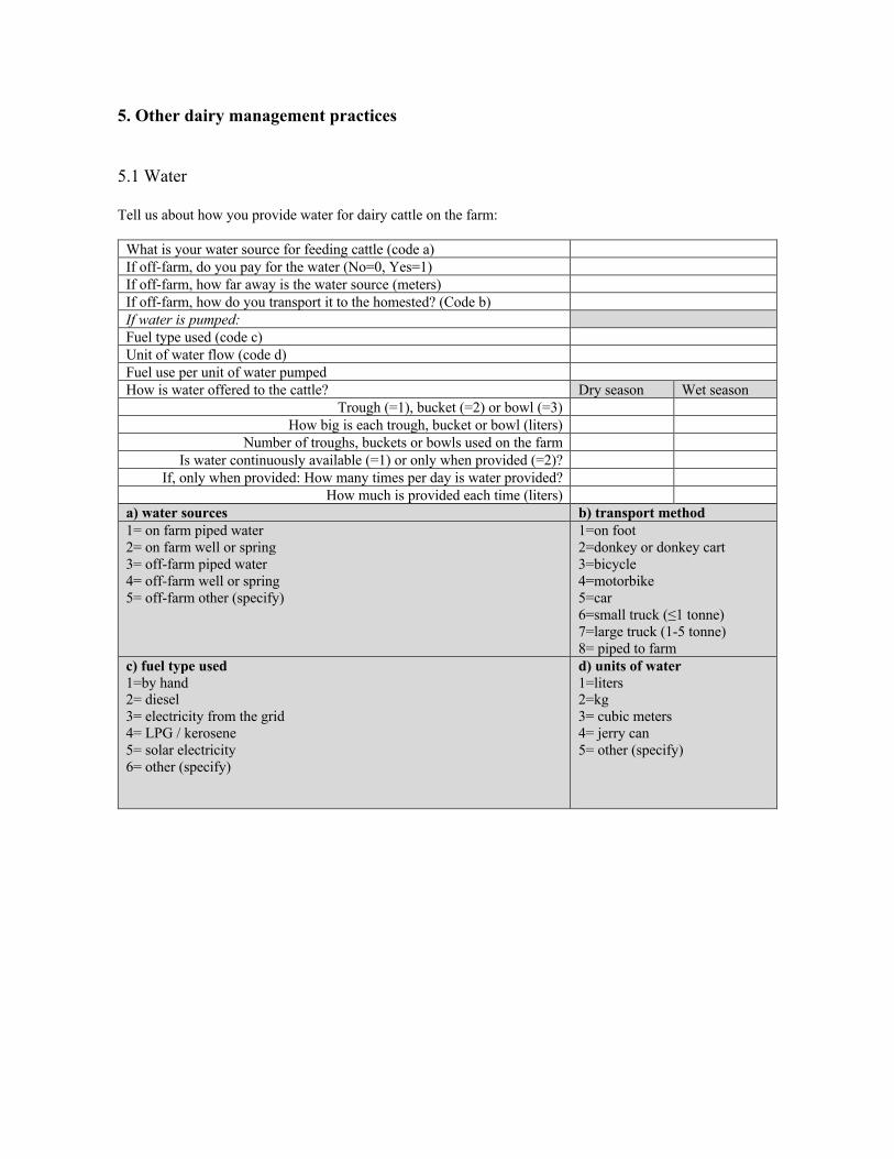
64

5. Other dairy management practices 5.1 Water Tell us about how you provide water for dairy cattle on the farm:

What is your water source for feeding cattle (code a) If off-farm, do you pay for the water (No=0, Yes=1) If off-farm, how far away is the water source (meters) If off-farm, how do you transport it to the homested? (Code b) If water is pumped: Fuel type used (code c) Unit of water flow (code d) Fuel use per unit of water pumped How is water offered to the cattle? Dry season Wet season

Trough (=1), bucket (=2) or bowl (=3) How big is each trough, bucket or bowl (liters)

Number of troughs, buckets or bowls used on the farm Is water continuously available (=1) or only when provided (=2)?

If, only when provided: How many times per day is water provided? How much is provided each time (liters)

a) water sources b) transport method 1= on farm piped water 2= on farm well or spring 3= off-farm piped water 4= off-farm well or spring 5= off-farm other (specify)

1=on foot 2=donkey or donkey cart 3=bicycle 4=motorbike 5=car 6=small truck (≤1 tonne) 7=large truck (1-5 tonne) 8= piped to farm

c) fuel type used 1=by hand 2= diesel 3= electricity from the grid 4= LPG / kerosene 5= solar electricity 6= other (specify)

d) units of water 1=liters 2=kg 3= cubic meters 4= jerry can 5= other (specify)

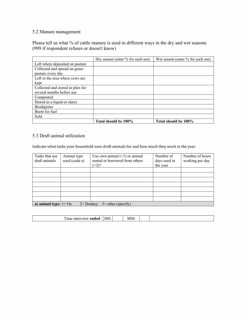
65

5.2 Manure management Please tell us what % of cattle manure is used in different ways in the dry and wet seasons (999 if respondent refuses or doesn't know)

Dry season (enter % for each use) Wet season (enter % for each use) Left where deposited on pasture Collected and spread on grass/ pasture every day

Left in the area where cows are kept

Collected and stored in piles for several months before use

Composted Stored as a liquid or slurry Biodigester Burnt for fuel Sold Total should be 100% Total should be 100%

5.3 Draft animal utilization Indicatewhattasksyourhouseholdusesdraftanimalsforandhowmuchtheyworkintheyear.

Tasks that use draft animals

Animal type used (code a)

Use own animal (=1) or animal rented or borrowed from others (=2)?

Number of days used in the year

Number of hours working per day

a) animal type: 1= Ox 2= Donkey 3= other (specify)

Time interview ended : HH: MM:

66

To be answered privately by the enumerator immediately following the interview

1. In your opinion, how did you establish rapport with this respondent [____] 1 = with ease 2 = with some persuasion 3 = with difficulty 4 = it was impossible

2. Overall, how did the respondent give answers to your questions? [____] 1 = willingly 2 = reluctantly 3 = with persuasion 4 = it was hard to get answers

3. How often do you think the respondent was telling the truth? [____] 1 = rarely 2 = sometimes 3 = most of the times 4 = all the time

I certify that I have checked the questionnaire two times to be sure that all the questions have been answered, and that the answers are legible. Signed: _____________________ Date ____/____/____

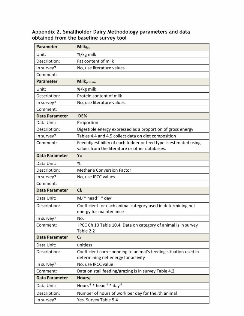
67

Appendix 2. Smallholder Dairy Methodology parameters and data obtained from the baseline survey tool

Parameter Milkfat Unit: %/kg milk Description: Fat content of milk In survey? No, use literature values. Comment: Parameter Milkprotein Unit: %/kg milk Description: Protein content of milk In survey? No, use literature values. Comment: Data Parameter DE% Data Unit: Proportion Description: Digestible energy expressed as a proportion of gross energy In survey? Tables 4.4 and 4.5 collect data on diet composition Comment: Feed digestibility of each fodder or feed type is estimated using

values from the literature or other databases. Data Parameter YM Data Unit: % Description: Methane Conversion Factor In survey? No, use IPCC values. Comment: Data Parameter Cfi Data Unit: MJ * head-1 * day- Description: Coefficient for each animal category used in determining net

energy for maintenance In survey? No. Comment: IPCC Ch 10 Table 10.4. Data on category of animal is in survey

Table 2.2 Data Parameter Ca Data Unit: unitless Description: Coefficient corresponding to animal’s feeding situation used in

determining net energy for activity In survey? No. use IPCC value Comment: Data on stall feeding/grazing is in survey Table 4.2 Data Parameter Hoursi Data Unit: Hours-1 * head-1 * day-1 Description: Number of hours of work per day for the ith animal In survey? Yes. Survey Table 5.4

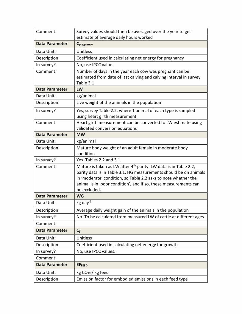
68

Comment: Survey values should then be averaged over the year to get estimate of average daily hours worked

Data Parameter Cpregnancy Data Unit: Unitless Description: Coefficient used in calculating net energy for pregnancy In survey? No, use IPCC value. Comment: Number of days in the year each cow was pregnant can be

estimated from date of last calving and calving interval in survey Table 3.1

Data Parameter LW Data Unit: kg/animal Description: Live weight of the animals in the population

In survey? Yes, survey Table 2.2, where 1 animal of each type is sampled using heart girth measurement.

Comment: Heart girth measurement can be converted to LW estimate using validated conversion equations

Data Parameter MW Data Unit: kg/animal Description: Mature body weight of an adult female in moderate body

condition In survey? Yes. Tables 2.2 and 3.1 Comment: Mature is taken as LW after 4th parity. LW data is in Table 2.2,

parity data is in Table 3.1. HG measurements should be on animals in ‘moderate’ condition, so Table 2.2 asks to note whether the animal is in ‘poor condition’, and if so, these measurements can be excluded.

Data Parameter WG Data Unit: kg day-1 Description: Average daily weight gain of the animals in the population In survey? No. To be calculated from measured LW of cattle at different ages Comment: Data Parameter Cg Data Unit: Unitless Description: Coefficient used in calculating net energy for growth In survey? No, use IPCC values. Comment: Data Parameter EFFEED Data Unit: kg CO2e/ kg feed Description: Emission factor for embodied emissions in each feed type

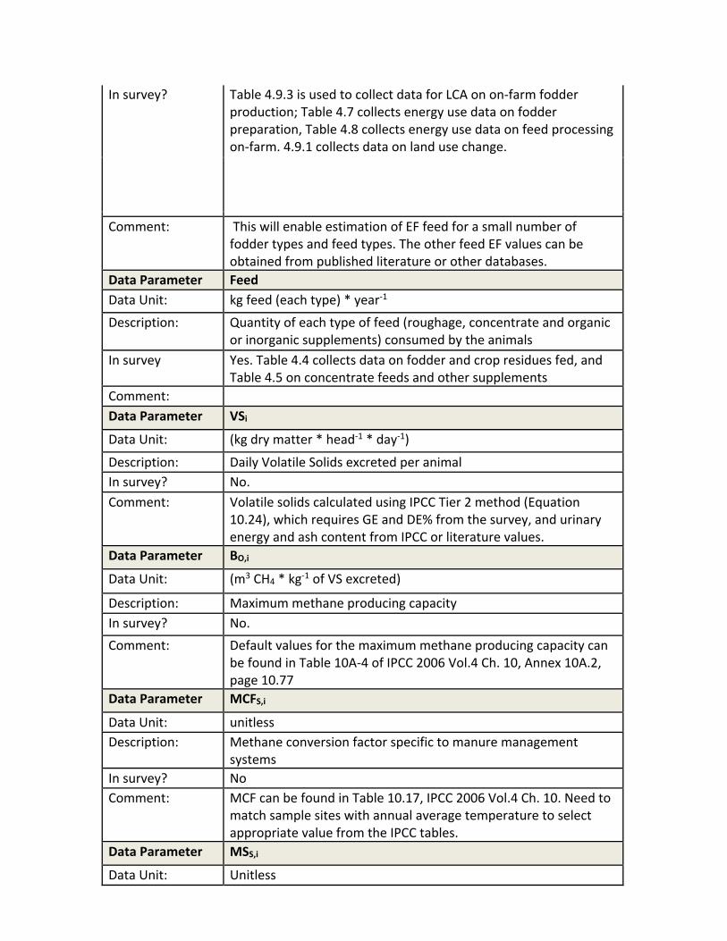
69

In survey? Table 4.9.3 is used to collect data for LCA on on-farm fodder production; Table 4.7 collects energy use data on fodder preparation, Table 4.8 collects energy use data on feed processing on-farm. 4.9.1 collects data on land use change.

Comment: This will enable estimation of EF feed for a small number of

fodder types and feed types. The other feed EF values can be obtained from published literature or other databases.

Data Parameter Feed Data Unit: kg feed (each type) * year-1 Description: Quantity of each type of feed (roughage, concentrate and organic

or inorganic supplements) consumed by the animals In survey Yes. Table 4.4 collects data on fodder and crop residues fed, and

Table 4.5 on concentrate feeds and other supplements Comment: Data Parameter VSi Data Unit: (kg dry matter * head-1 * day-1) Description: Daily Volatile Solids excreted per animal In survey? No. Comment: Volatile solids calculated using IPCC Tier 2 method (Equation

10.24), which requires GE and DE% from the survey, and urinary energy and ash content from IPCC or literature values.

Data Parameter BO,i Data Unit: (m3 CH4 * kg-1 of VS excreted)

Description: Maximum methane producing capacity In survey? No. Comment: Default values for the maximum methane producing capacity can

be found in Table 10A-4 of IPCC 2006 Vol.4 Ch. 10, Annex 10A.2, page 10.77

Data Parameter MCFS,i Data Unit: unitless Description: Methane conversion factor specific to manure management

systems In survey? No Comment: MCF can be found in Table 10.17, IPCC 2006 Vol.4 Ch. 10. Need to

match sample sites with annual average temperature to select appropriate value from the IPCC tables.

Data Parameter MSS,i Data Unit: Unitless

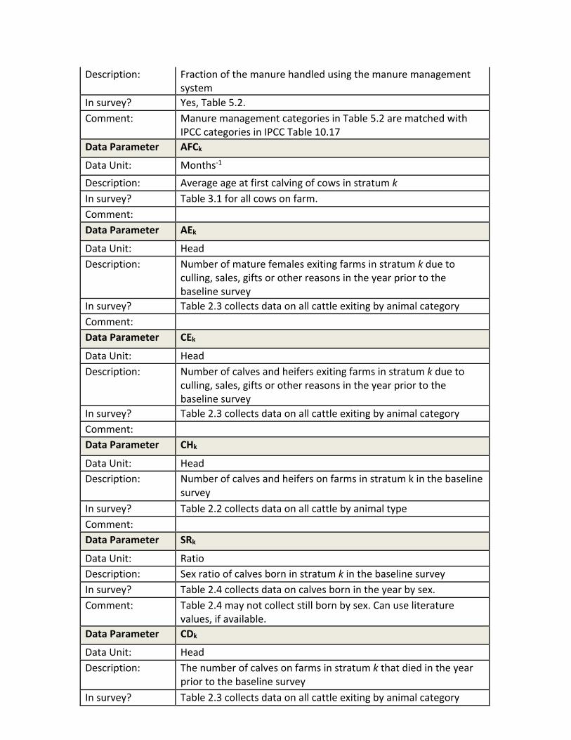
70

Description: Fraction of the manure handled using the manure management system

In survey? Yes, Table 5.2. Comment: Manure management categories in Table 5.2 are matched with

IPCC categories in IPCC Table 10.17 Data Parameter AFCk Data Unit: Months-1 Description: Average age at first calving of cows in stratum k In survey? Table 3.1 for all cows on farm. Comment:

Data Parameter AEk Data Unit: Head Description: Number of mature females exiting farms in stratum k due to

culling, sales, gifts or other reasons in the year prior to the baseline survey

In survey? Table 2.3 collects data on all cattle exiting by animal category Comment:

Data Parameter CEk Data Unit: Head Description: Number of calves and heifers exiting farms in stratum k due to

culling, sales, gifts or other reasons in the year prior to the baseline survey

In survey? Table 2.3 collects data on all cattle exiting by animal category Comment:

Data Parameter CHk Data Unit: Head Description: Number of calves and heifers on farms in stratum k in the baseline

survey In survey? Table 2.2 collects data on all cattle by animal type Comment:

Data Parameter SRk Data Unit: Ratio Description: Sex ratio of calves born in stratum k in the baseline survey In survey? Table 2.4 collects data on calves born in the year by sex. Comment: Table 2.4 may not collect still born by sex. Can use literature

values, if available. Data Parameter CDk Data Unit: Head Description: The number of calves on farms in stratum k that died in the year

prior to the baseline survey In survey? Table 2.3 collects data on all cattle exiting by animal category

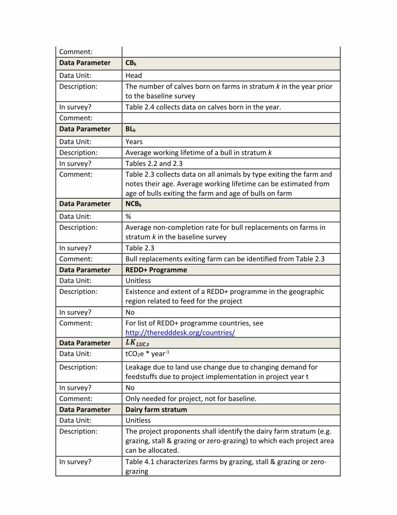
71

Comment:

Data Parameter CBk Data Unit: Head Description: The number of calves born on farms in stratum k in the year prior

to the baseline survey In survey? Table 2.4 collects data on calves born in the year. Comment:

Data Parameter BLk Data Unit: Years Description: Average working lifetime of a bull in stratum k In survey? Tables 2.2 and 2.3 Comment: Table 2.3 collects data on all animals by type exiting the farm and

notes their age. Average working lifetime can be estimated from age of bulls exiting the farm and age of bulls on farm

Data Parameter NCBk Data Unit: % Description: Average non-completion rate for bull replacements on farms in

stratum k in the baseline survey In survey? Table 2.3 Comment: Bull replacements exiting farm can be identified from Table 2.3 Data Parameter REDD+ Programme Data Unit: Unitless Description: Existence and extent of a REDD+ programme in the geographic

region related to feed for the project In survey? No Comment: For list of REDD+ programme countries, see

http://theredddesk.org/countries/ Data Parameter Data Unit: tCO2e * year-1

Description: Leakage due to land use change due to changing demand for

feedstuffs due to project implementation in project year t In survey? No Comment: Only needed for project, not for baseline. Data Parameter Dairy farm stratum Data Unit: Unitless Description: The project proponents shall identify the dairy farm stratum (e.g.

grazing, stall & grazing or zero-grazing) to which each project area can be allocated.

In survey? Table 4.1 characterizes farms by grazing, stall & grazing or zero-grazing

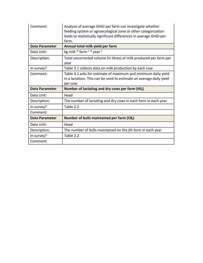
72

Comment: Analysis of average GHGI per farm can investigate whether feeding system or agroecological zone or other categorization leads to statistically significant differences in average GHGI per farm.

Data Parameter Annual total milk yield per farm Data Unit: kg milk * farm-1 * year-1 Description: Total uncorrected volume (in litres) of milk produced per farm per

year In survey? Table 3.1 collects data on milk production by each cow Comment: Table 3.1 asks for estimate of maximum and minimum daily yield

in a lactation. This can be used to estimate an average daily yield per cow.

Data Parameter Number of lactating and dry cows per farm (HSj) Data Unit: Head Description: The number of lactating and dry cows in each farm in each year In survey? Table 2.2 Comment:

Data Parameter Number of bulls maintained per farm (CBj) Data Unit: Head Description: The number of bulls maintained on the jth farm in each year In survey? Table 2.2 Comment:

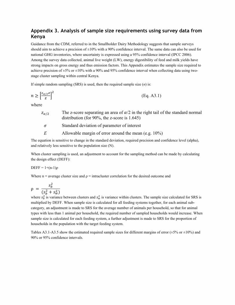
73

Appendix 3. Analysis of sample size requirements using survey data from Kenya Guidance from the CDM, referred to in the Smallholder Dairy Methodology suggests that sample surveys should aim to achieve a precision of ±10% with a 90% confidence interval. The same data can also be used for national GHG inventories, where uncertainty is expressed using a 95% confidence interval (IPCC 2006). Among the survey data collected, animal live weight (LW), energy digestibility of feed and milk yields have strong impacts on gross energy and thus emission factors. This Appendix estimates the sample size required to achieve precision of ±5% or ±10% with a 90% and 95% confidence interval when collecting data using two-stage cluster sampling within central Kenya.

If simple random sampling (SRS) is used, then the required sample size (n) is:

! ≥ #$%/'() *+ (Eq. A3.1)

where ,-/+ The z-score separating an area of ./2 in the right tail of the standard normal

distribution (for 90%, the z-score is 1.645)

/ Standard deviation of parameter of interest E Allowable margin of error around the mean (e.g. 10%)

The equation is sensitive to change in the standard deviation, required precision and confidence level (alpha), and relatively less sensitive to the population size (N).

When cluster sampling is used, an adjustment to account for the sampling method can be made by calculating the design effect (DEFF):

DEFF = 1+(n-1)ρ

Where n = average cluster size and ρ = intracluster correlation for the desired outcome and

ρ = 34+(34+ + 37+ )

where 34+ is variance between clusters and 37+ is variance within clusters. The sample size calculated for SRS is multiplied by DEFF. When sample size is calculated for all feeding systems together, for each animal sub-category, an adjustment is made to SRS for the average number of animals per household, so that for animal types with less than 1 animal per household, the required number of sampled households would increase. When sample size is calculated for each feeding system, a further adjustment is made to SRS for the proportion of households in the population with the target feeding system.

Tables A3.1-A3.5 show the estimated required sample sizes for different margins of error (±5% or ±10%) and 90% or 95% confidence intervals.

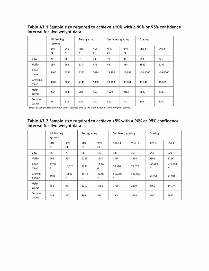
74

Table A3.1 Sample size required to achieve ±10% with a 90% or 95% confidence interval for live weight data

All feeding

systems

Zero-grazing Semi-zero grazing Grazing

90%

CI

95%

CI

90%

CI

95%

CI

90%

CI

95%

CI 90% CI 95% CI

Cow 20 28 31 43 79 94 250 321

Heifer 184 262 319 453 617 868 1529 2162

Adult

male 3406 4784 2287 3094 13,190 18,893 >20,000* >20,000*

Growing

male 4005 5650 4149 5890 21,789 30,761 13,240 18,656

Male

calves 252 353 703 967 1529 2162 3697 4930

Female

calves 91 125 131 180 501 701 802 1070

* required sample size could not be established due to the small sample size in the pilot survey.

Table A3.2 Sample size required to achieve ±5% with a 90% or 95% confidence interval for live weight data

All feeding

systems Zero-grazing Semi-zero grazing Grazing

90%

CI

95%

CI

90%

CI

95%

CI 90% CI 95% CI 90% CI 95% CI

Cow 55 75 86 123 189 251 643 929

Heifer 702 993 1225 1730 2334 3298 5801 8226

Adult

male

12,974

18,326 7936 11,164

50,620 71,652 >75,000*

>75,000*

Growin

g male 1996

>2000*

15,795

22,487

>16,000*

>22,500*

50,551 71,916

Male

calves 655 957 1319 1759 1755 2339 9860 14,174

Female

calves 283 397 394 558 1603 2254 2140 2942

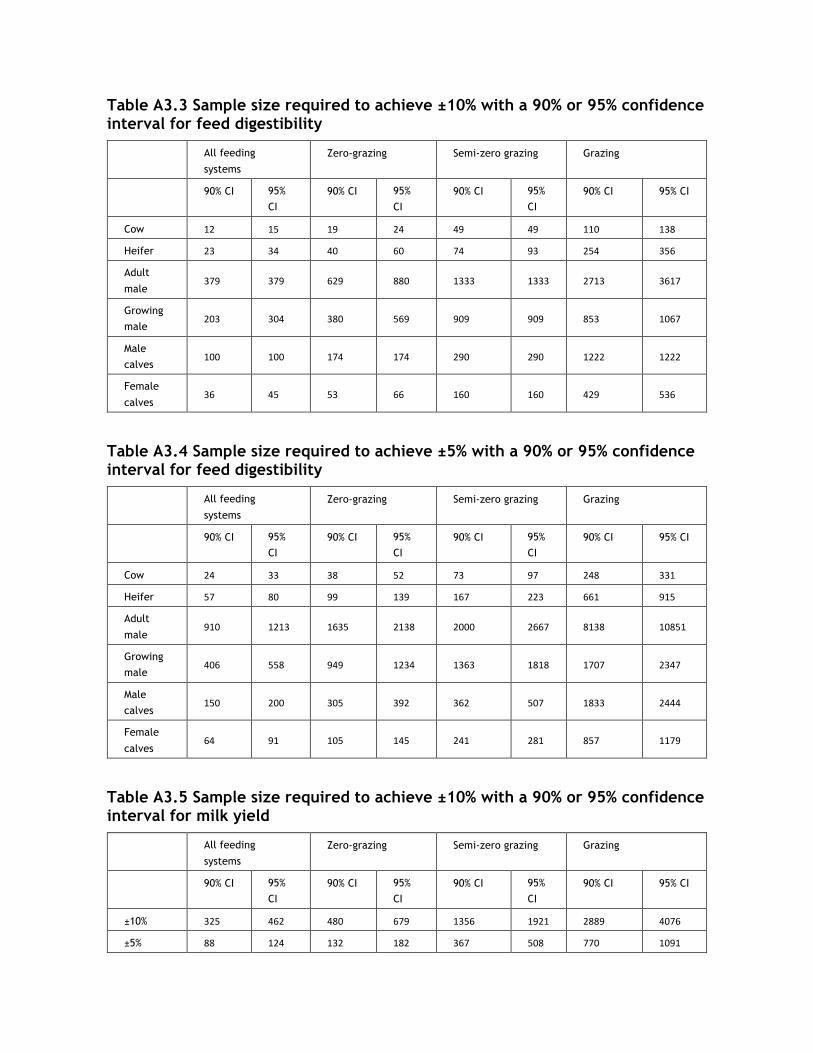
75

Table A3.3 Sample size required to achieve ±10% with a 90% or 95% confidence interval for feed digestibility

All feeding

systems


90% CI 95%

CI 90% CI 95%

CI 90% CI 95%

CI 90% CI 95% CI

Cow 12 15 19 24 49 49 110 138

Heifer 23 34 40 60 74 93 254 356

Adult

male 379 379 629 880 1333 1333 2713 3617

Growing

male 203 304 380 569 909 909 853 1067

Male

calves 100 100 174 174 290 290 1222 1222

Female

calves 36 45 53 66 160 160 429 536

Table A3.4 Sample size required to achieve ±5% with a 90% or 95% confidence interval for feed digestibility

All feeding

systems


90% CI 95%

CI 90% CI 95%

CI 90% CI 95%

CI 90% CI 95% CI

Cow 24 33 38 52 73 97 248 331

Heifer 57 80 99 139 167 223 661 915

Adult

male 910 1213 1635 2138 2000 2667 8138 10851

Growing

male 406 558 949 1234 1363 1818 1707 2347

Male

calves 150 200 305 392 362 507 1833 2444

Female

calves 64 91 105 145 241 281 857 1179

Table A3.5 Sample size required to achieve ±10% with a 90% or 95% confidence interval for milk yield

All feeding

systems


90% CI 95%

CI 90% CI 95%

CI 90% CI 95%

CI 90% CI 95% CI

±10% 325 462 480 679 1356 1921 2889 4076

±5% 88 124 132 182 367 508 770 1091

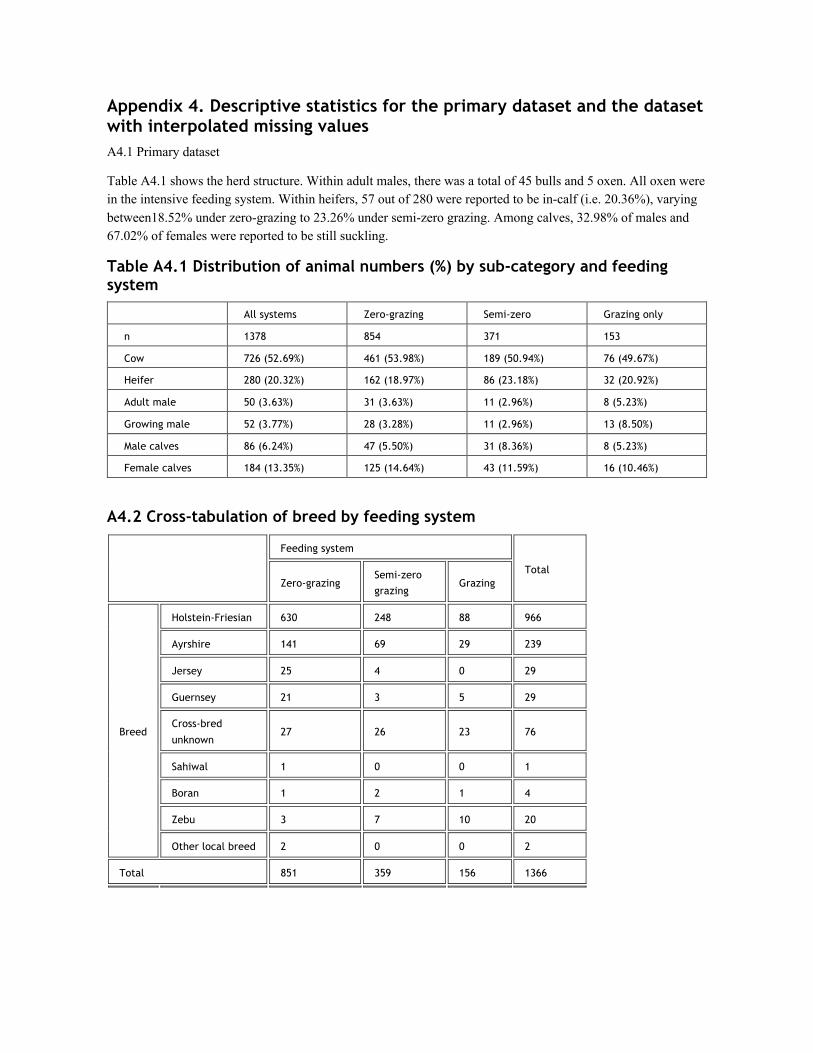
76

Appendix 4. Descriptive statistics for the primary dataset and the dataset with interpolated missing values A4.1 Primary dataset

Table A4.1 shows the herd structure. Within adult males, there was a total of 45 bulls and 5 oxen. All oxen were in the intensive feeding system. Within heifers, 57 out of 280 were reported to be in-calf (i.e. 20.36%), varying between18.52% under zero-grazing to 23.26% under semi-zero grazing. Among calves, 32.98% of males and 67.02% of females were reported to be still suckling.

Table A4.1 Distribution of animal numbers (%) by sub-category and feeding system

All systems Zero-grazing Semi-zero Grazing only

n 1378 854 371 153

Cow 726 (52.69%) 461 (53.98%) 189 (50.94%) 76 (49.67%)

Heifer 280 (20.32%) 162 (18.97%) 86 (23.18%) 32 (20.92%)

Adult male 50 (3.63%) 31 (3.63%) 11 (2.96%) 8 (5.23%)

Growing male 52 (3.77%) 28 (3.28%) 11 (2.96%) 13 (8.50%)

Male calves 86 (6.24%) 47 (5.50%) 31 (8.36%) 8 (5.23%)

Female calves 184 (13.35%) 125 (14.64%) 43 (11.59%) 16 (10.46%)

A4.2 Cross-tabulation of breed by feeding system

Feeding system

Total Zero-grazing

Semi-zero

grazing Grazing

Breed

Holstein-Friesian 630 248 88 966

Ayrshire 141 69 29 239

Jersey 25 4 0 29

Guernsey 21 3 5 29

Cross-bred

unknown 27 26 23 76

Sahiwal 1 0 0 1

Boran 1 2 1 4

Zebu 3 7 10 20

Other local breed 2 0 0 2

Total 851 359 156 1366

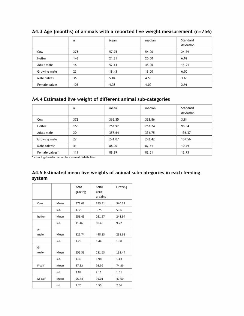
77

A4.3 Age (months) of animals with a reported live weight measurement (n=756)

n Mean median Standard

deviation

Cow 275 57.75 54.00 24.39

Heifer 146 21.31 20.00 6.92

Adult male 16 52.13 48.00 15.91

Growing male 23 18.43 18.00 6.00

Male calves 36 5.04 4.50 3.63

Female calves 102 4.38 4.00 2.91

A4.4 Estimated live weight of different animal sub-categories

n mean median Standard

deviation

Cow 372 365.35 363.86 3.84

Heifer 166 262.92 263.74 98.34

Adult male 20 357.64 334.75 136.37

Growing male 27 241.07 242.42 107.56

Male calves* 41 88.00 82.51 10.79

Female calves* 111 88.29 82.51 12.73 * after log-transformation to a normal distribution.

A4.5 Estimated mean live weights of animal sub-categories in each feeding system

Zero-

grazing Semi-

zero

grazing

Grazing

Cow Mean 371.62 353.91 340.21

s.d. 4.38 3.75 5.06

heifer Mean 256.49 261.67 243.94

s.d. 11.46 10.48 9.22

A-male Mean 321.74 448.33 231.63

s.d. 1.29 1.44 1.98

G-male Mean 255.33 231.63 133.44

s.d. 1.39 1.98 1.43

F-calf Mean 87.32 98.99 74.89

s.d. 1.89 2.11 1.61

M-calf Mean 95.74 91.01 47.60

s.d. 1.70 1.55 2.66

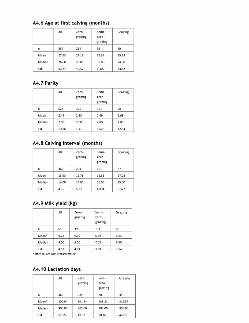
78

A4.6 Age at first calving (months)

All Zero-

grazing Semi-

zero

grazing

Grazing

n 357 235 93 29

Mean 27.63 27.16 29.34 25.93

Median 26.00 26.00 30.00 24.00

s.d. 5.127 4.957 5.309 4.652

A4.7 Parity

All Zero-

grazing Semi-

zero

grazing

Grazing

n 624 395 161 68

Mean 2.44 2.38 2.49 2.63

Median 2.00 2.00 2.00 2.00

s.d. 1.486 1.41 1.628 1.564

A4.8 Calving interval (months)

All Zero-

grazing Semi-

zero

grazing

Grazing

n 362 224 101 37

Mean 15.93 15.78 15.83 17.08

Median 14.00 14.00 15.00 15.00

s.d. 4.95 5.22 4.094 5.372

A4.9 Milk yield (kg)

All Zero-

grazing Semi-

zero

grazing

Grazing

n 616 396 154 66

Mean* 8.21 9.00 6.99 6.63

Median 8.00 8.50 7.03 6.50

s.d. 4.51 4.71 3.98 3.54 * after square root transformation

A4.10 Lactation days

All Zero-

grazing Semi-

zero

grazing

Grazing

n 360 245 80 35

Mean* 300.04 301.54 288.21 316.57

Median 305.00 305.00 305.00 305.00

s.d. 57.55 49.52 80.16 42.67

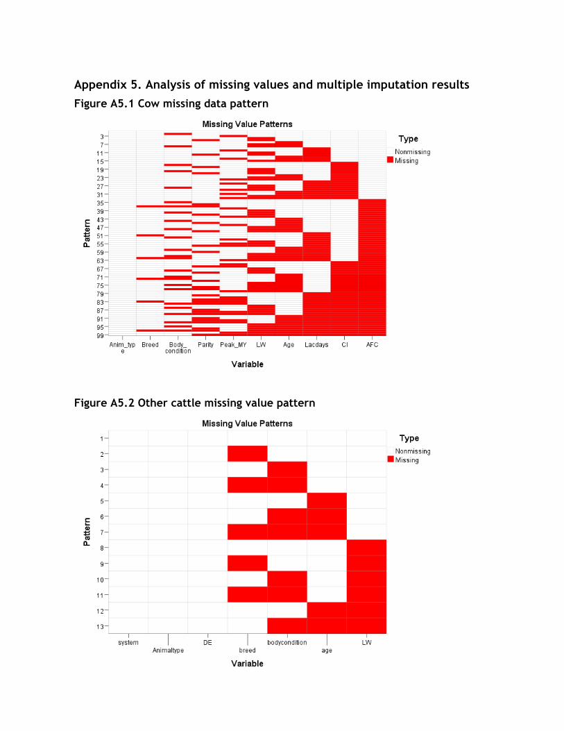
79

Appendix 5. Analysis of missing values and multiple imputation results Figure A5.1 Cow missing data pattern

Figure A5.2 Other cattle missing value pattern

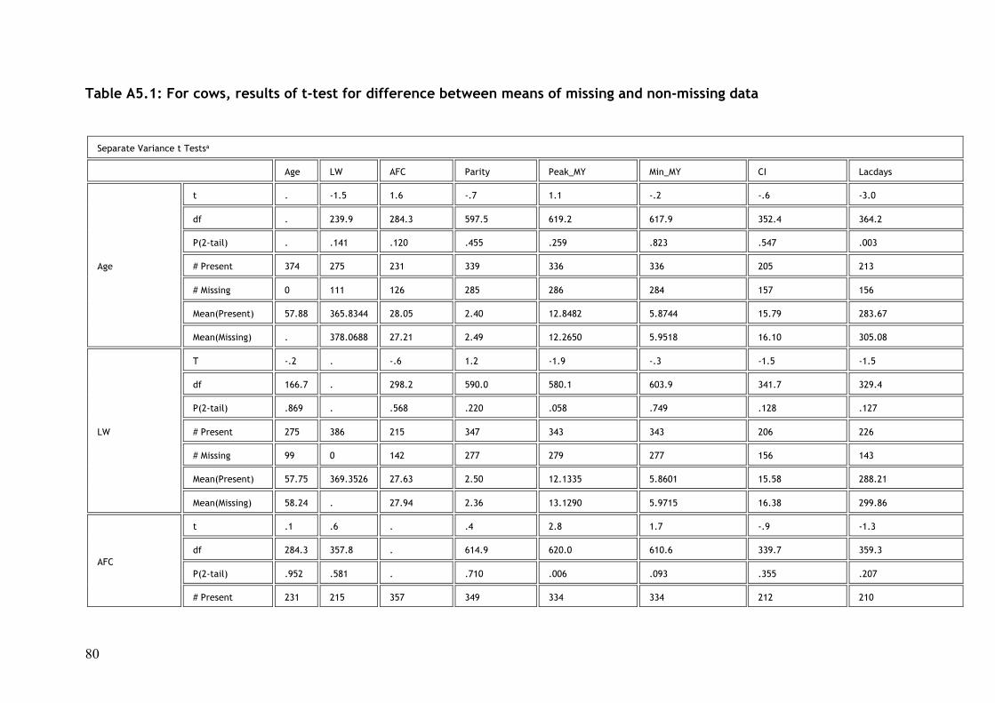
80

Table A5.1: For cows, results of t-test for difference between means of missing and non-missing data

Separate Variance t Testsa

Age LW AFC Parity Peak_MY Min_MY CI Lacdays

Age

t . -1.5 1.6 -.7 1.1 -.2 -.6 -3.0

df . 239.9 284.3 597.5 619.2 617.9 352.4 364.2

P(2-tail) . .141 .120 .455 .259 .823 .547 .003

# Present 374 275 231 339 336 336 205 213

# Missing 0 111 126 285 286 284 157 156

Mean(Present) 57.88 365.8344 28.05 2.40 12.8482 5.8744 15.79 283.67

Mean(Missing) . 378.0688 27.21 2.49 12.2650 5.9518 16.10 305.08

LW

T -.2 . -.6 1.2 -1.9 -.3 -1.5 -1.5

df 166.7 . 298.2 590.0 580.1 603.9 341.7 329.4

P(2-tail) .869 . .568 .220 .058 .749 .128 .127

# Present 275 386 215 347 343 343 206 226

# Missing 99 0 142 277 279 277 156 143

Mean(Present) 57.75 369.3526 27.63 2.50 12.1335 5.8601 15.58 288.21

Mean(Missing) 58.24 . 27.94 2.36 13.1290 5.9715 16.38 299.86

AFC

t .1 .6 . .4 2.8 1.7 -.9 -1.3

df 284.3 357.8 . 614.9 620.0 610.6 339.7 359.3

P(2-tail) .952 .581 . .710 .006 .093 .355 .207

# Present 231 215 357 349 334 334 212 210

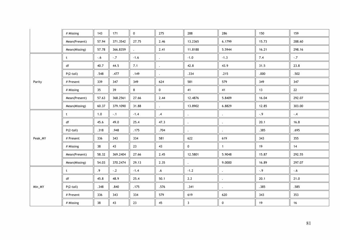
81

# Missing 143 171 0 275 288 286 150 159

Mean(Present) 57.94 371.3542 27.75 2.46 13.2365 6.1799 15.73 288.60

Mean(Missing) 57.78 366.8359 . 2.41 11.8188 5.5944 16.21 298.16

Parity

t -.6 -.7 -1.6 . -1.0 -1.3 7.4 -.7

df 40.7 44.5 7.1 . 42.8 43.9 31.5 23.8

P(2-tail) .548 .477 .149 . .334 .215 .000 .502

# Present 339 347 349 624 581 579 349 347

# Missing 35 39 8 0 41 41 13 22

Mean(Present) 57.63 368.2561 27.66 2.44 12.4876 5.8409 16.04 292.07

Mean(Missing) 60.37 379.1090 31.88 . 13.8902 6.8829 12.85 303.00

Peak_MY

t 1.0 -.1 -1.4 .4 . . -.9 -.4

df 45.6 49.0 25.4 47.3 . . 20.1 16.8

P(2-tail) .318 .948 .175 .704 . . .385 .695

# Present 336 343 334 581 622 619 343 355

# Missing 38 43 23 43 0 1 19 14

Mean(Present) 58.32 369.2404 27.66 2.45 12.5801 5.9048 15.87 292.55

Mean(Missing) 54.03 370.2474 29.13 2.35 . 9.0000 16.89 297.07

Min_MY

t .9 -.2 -1.4 .6 -1.2 . -.9 -.6

df 45.8 48.9 25.4 50.1 2.2 . 20.1 21.0

P(2-tail) .348 .840 .175 .576 .341 . .385 .585

# Present 336 343 334 579 619 620 343 353

# Missing 38 43 23 45 3 0 19 16

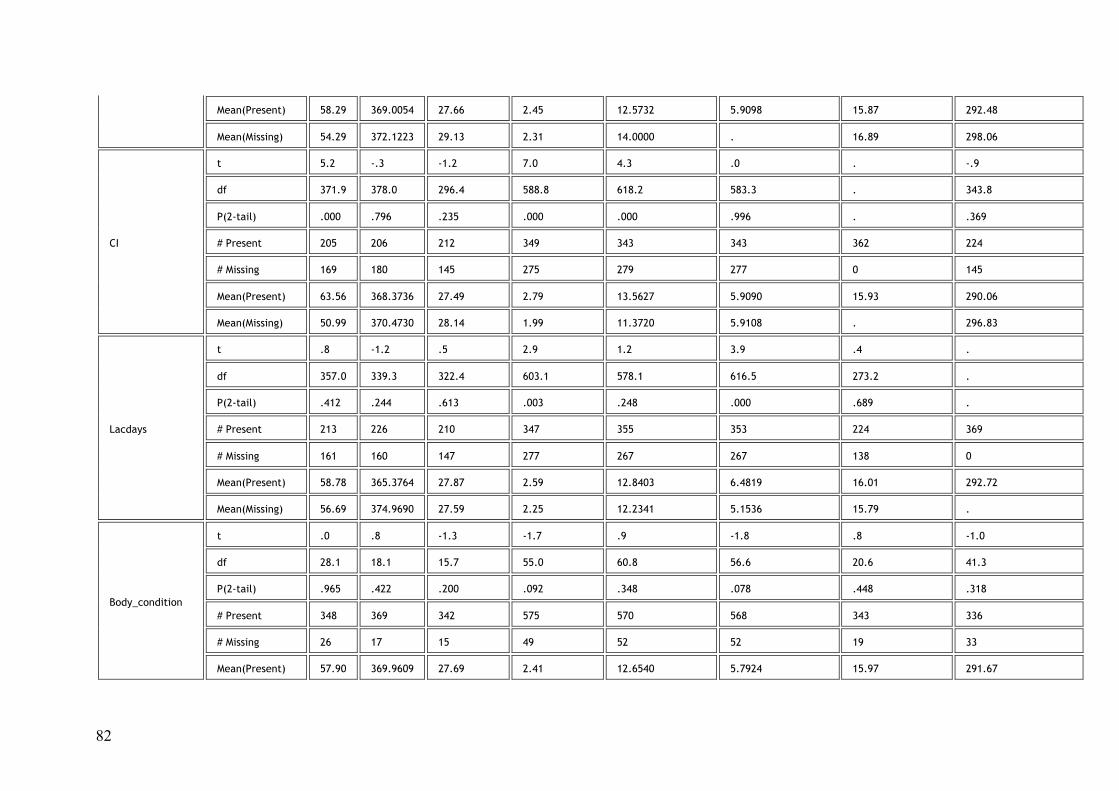
82

Mean(Present) 58.29 369.0054 27.66 2.45 12.5732 5.9098 15.87 292.48

Mean(Missing) 54.29 372.1223 29.13 2.31 14.0000 . 16.89 298.06

CI

t 5.2 -.3 -1.2 7.0 4.3 .0 . -.9

df 371.9 378.0 296.4 588.8 618.2 583.3 . 343.8

P(2-tail) .000 .796 .235 .000 .000 .996 . .369

# Present 205 206 212 349 343 343 362 224

# Missing 169 180 145 275 279 277 0 145

Mean(Present) 63.56 368.3736 27.49 2.79 13.5627 5.9090 15.93 290.06

Mean(Missing) 50.99 370.4730 28.14 1.99 11.3720 5.9108 . 296.83

Lacdays

t .8 -1.2 .5 2.9 1.2 3.9 .4 .

df 357.0 339.3 322.4 603.1 578.1 616.5 273.2 .

P(2-tail) .412 .244 .613 .003 .248 .000 .689 .

# Present 213 226 210 347 355 353 224 369

# Missing 161 160 147 277 267 267 138 0

Mean(Present) 58.78 365.3764 27.87 2.59 12.8403 6.4819 16.01 292.72

Mean(Missing) 56.69 374.9690 27.59 2.25 12.2341 5.1536 15.79 .

Body_condition

t .0 .8 -1.3 -1.7 .9 -1.8 .8 -1.0

df 28.1 18.1 15.7 55.0 60.8 56.6 20.6 41.3

P(2-tail) .965 .422 .200 .092 .348 .078 .448 .318

# Present 348 369 342 575 570 568 343 336

# Missing 26 17 15 49 52 52 19 33

Mean(Present) 57.90 369.9609 27.69 2.41 12.6540 5.7924 15.97 291.67

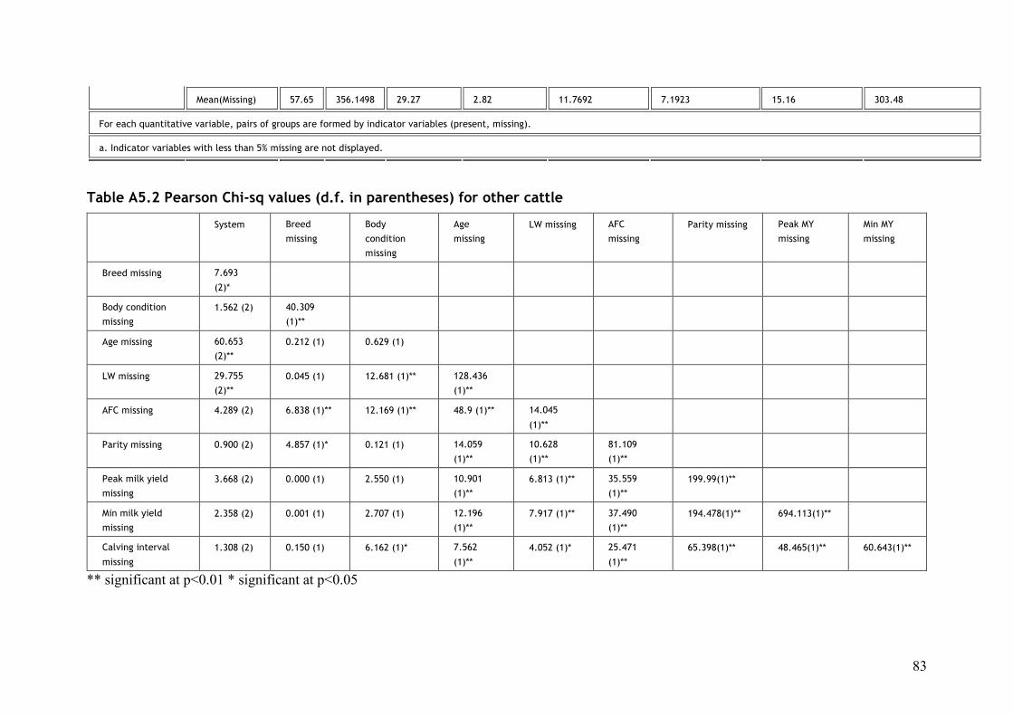
83

Table A5.2 Pearson Chi-sq values (d.f. in parentheses) for other cattle

System Breed

missing

Body

condition

missing

Age

missing

LW missing AFC

missing

Parity missing Peak MY

missing

Min MY

missing

Breed missing 7.693

(2)*

Body condition

missing

1.562 (2) 40.309

(1)**

Age missing 60.653

(2)**

0.212 (1) 0.629 (1)

LW missing 29.755

(2)**

0.045 (1) 12.681 (1)** 128.436

(1)**

AFC missing 4.289 (2) 6.838 (1)** 12.169 (1)** 48.9 (1)** 14.045

(1)**

Parity missing 0.900 (2) 4.857 (1)* 0.121 (1) 14.059

(1)**

10.628

(1)**

81.109

(1)**

Peak milk yield

missing

3.668 (2) 0.000 (1) 2.550 (1) 10.901

(1)**

6.813 (1)** 35.559

(1)**

199.99(1)**

Min milk yield

missing

2.358 (2) 0.001 (1) 2.707 (1) 12.196

(1)**

7.917 (1)** 37.490

(1)**

194.478(1)** 694.113(1)**

Calving interval

missing

1.308 (2) 0.150 (1) 6.162 (1)* 7.562

(1)**

4.052 (1)* 25.471

(1)**

65.398(1)** 48.465(1)** 60.643(1)**

** significant at p<0.01 * significant at p<0.05

Mean(Missing) 57.65 356.1498 29.27 2.82 11.7692 7.1923 15.16 303.48

For each quantitative variable, pairs of groups are formed by indicator variables (present, missing).

a. Indicator variables with less than 5% missing are not displayed.

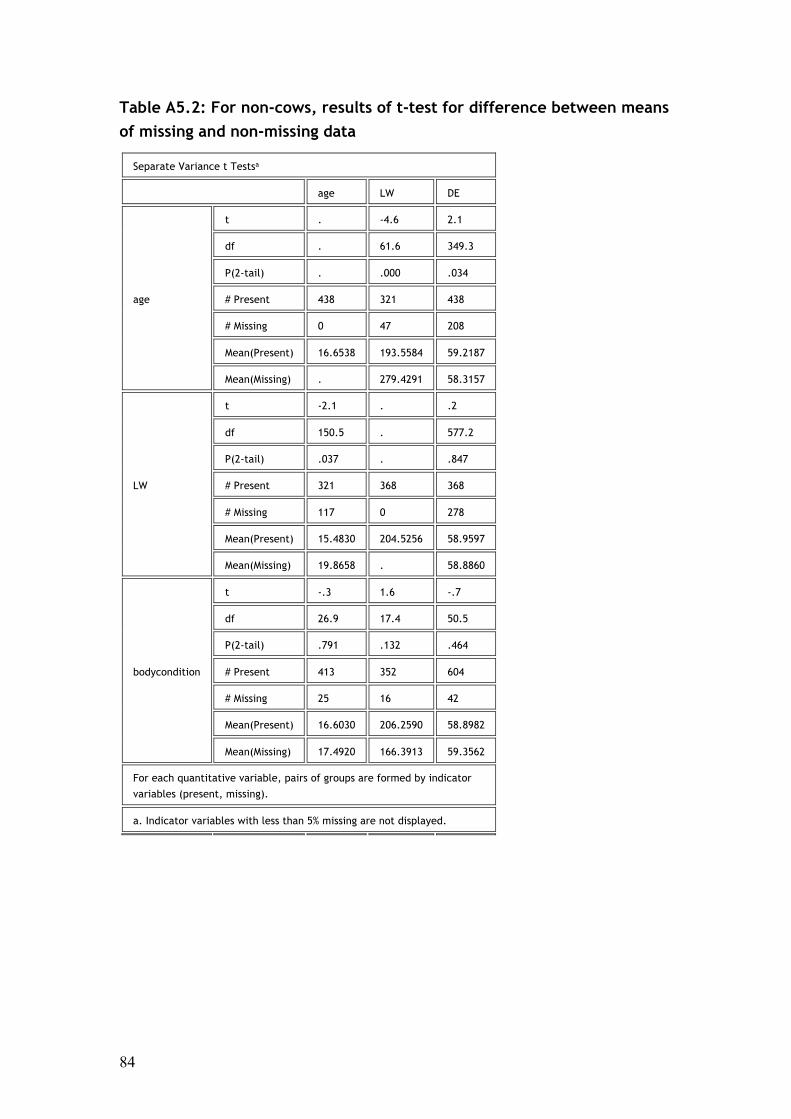
84

Table A5.2: For non-cows, results of t-test for difference between means

of missing and non-missing data

Separate Variance t Testsa

age LW DE

age

t . -4.6 2.1

df . 61.6 349.3

P(2-tail) . .000 .034

# Present 438 321 438

# Missing 0 47 208

Mean(Present) 16.6538 193.5584 59.2187

Mean(Missing) . 279.4291 58.3157

LW

t -2.1 . .2

df 150.5 . 577.2

P(2-tail) .037 . .847

# Present 321 368 368

# Missing 117 0 278

Mean(Present) 15.4830 204.5256 58.9597

Mean(Missing) 19.8658 . 58.8860

bodycondition

t -.3 1.6 -.7

df 26.9 17.4 50.5

P(2-tail) .791 .132 .464

# Present 413 352 604

# Missing 25 16 42

Mean(Present) 16.6030 206.2590 58.8982

Mean(Missing) 17.4920 166.3913 59.3562

For each quantitative variable, pairs of groups are formed by indicator

variables (present, missing).

a. Indicator variables with less than 5% missing are not displayed.

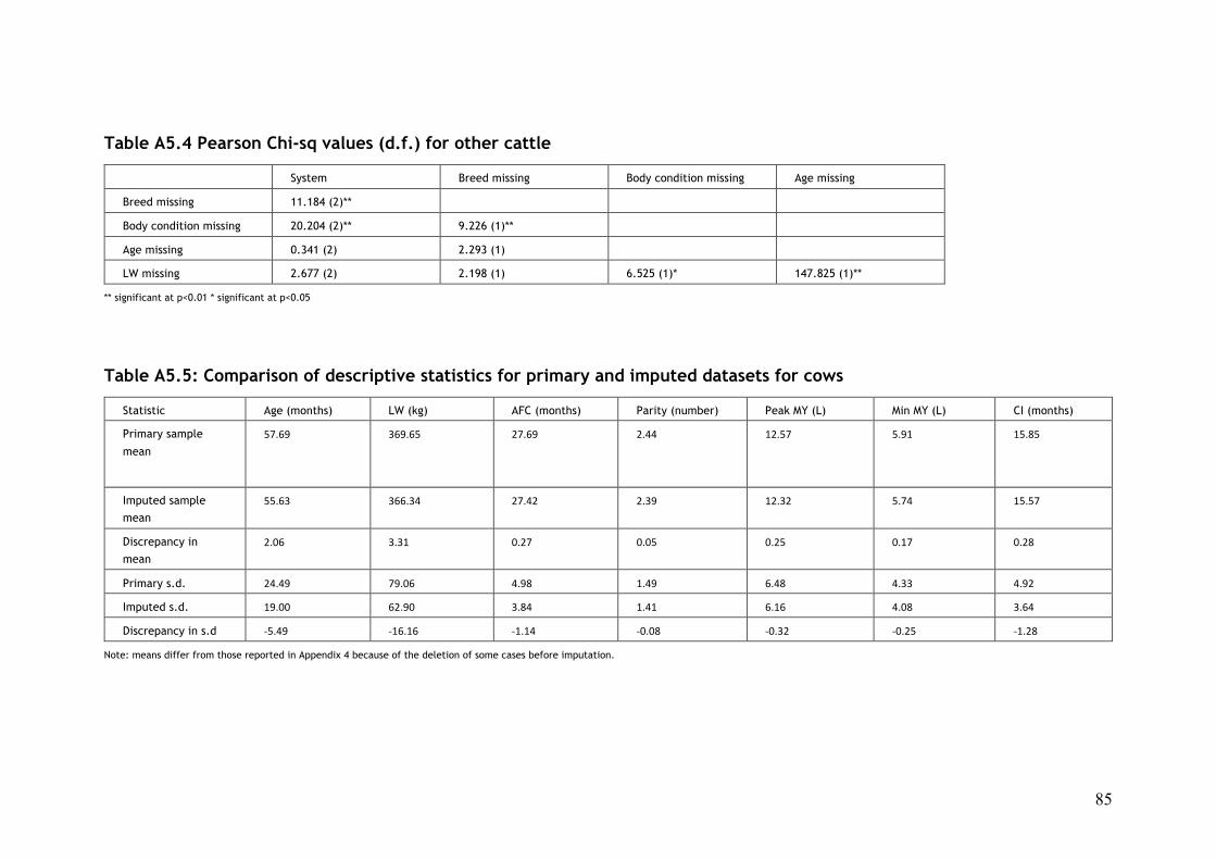
85

Table A5.4 Pearson Chi-sq values (d.f.) for other cattle

System Breed missing Body condition missing Age missing

Breed missing 11.184 (2)**

Body condition missing 20.204 (2)** 9.226 (1)**

Age missing 0.341 (2) 2.293 (1)

LW missing 2.677 (2) 2.198 (1) 6.525 (1)* 147.825 (1)**

** significant at p<0.01 * significant at p<0.05

Table A5.5: Comparison of descriptive statistics for primary and imputed datasets for cows

Statistic Age (months) LW (kg) AFC (months) Parity (number) Peak MY (L) Min MY (L) CI (months)

Primary sample

mean

57.69 369.65 27.69 2.44 12.57 5.91 15.85

Imputed sample

mean 55.63 366.34 27.42 2.39 12.32 5.74 15.57

Discrepancy in

mean 2.06 3.31 0.27 0.05 0.25 0.17 0.28

Primary s.d. 24.49 79.06 4.98 1.49 6.48 4.33 4.92

Imputed s.d. 19.00 62.90 3.84 1.41 6.16 4.08 3.64

Discrepancy in s.d -5.49 -16.16 -1.14 -0.08 -0.32 -0.25 -1.28

Note: means differ from those reported in Appendix 4 because of the deletion of some cases before imputation.

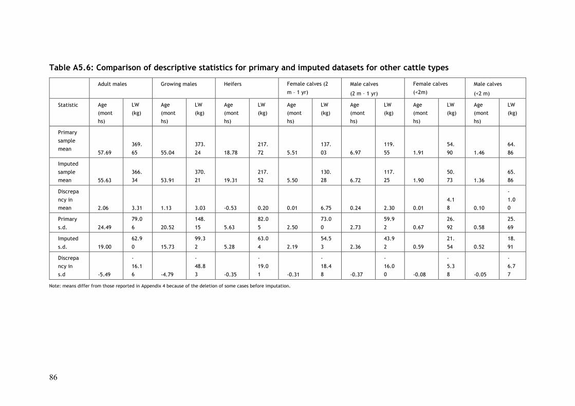
86

Table A5.6: Comparison of descriptive statistics for primary and imputed datasets for other cattle types

Adult males Growing males Heifers Female calves (2

m – 1 yr)

Male calves

(2 m – 1 yr)

Female calves

(<2m)

Male calves

(<2 m)

Statistic Age

(mont

hs)

LW

(kg)

Age

(mont

hs)

LW

(kg)

Age

(mont

hs)

LW

(kg)

Age

(mont

hs)

LW

(kg)

Age

(mont

hs)

LW

(kg)

Age

(mont

hs)

LW

(kg)

Age

(mont

hs)

LW

(kg)

Primary

sample

mean 57.69

369.

65 55.04

373.

24 18.78

217.

72 5.51

137.

03 6.97

119.

55 1.91

54.

90 1.46

64.

86

Imputed

sample

mean 55.63

366.

34 53.91

370.

21 19.31

217.

52 5.50

130.

28 6.72

117.

25 1.90

50.

73 1.36

65.

86

Discrepa

ncy in

mean 2.06 3.31 1.13 3.03 -0.53 0.20 0.01 6.75 0.24 2.30 0.01

4.1

8 0.10

-

1.0

0

Primary

s.d. 24.49

79.0

6 20.52

148.

15 5.63

82.0

5 2.50

73.0

0 2.73

59.9

2 0.67

26.

92 0.58

25.

69

Imputed

s.d. 19.00

62.9

0 15.73

99.3

2 5.28

63.0

4 2.19

54.5

3 2.36

43.9

2 0.59

21.

54 0.52

18.

91

Discrepa

ncy in

s.d -5.49

-

16.1

6 -4.79

-

48.8

3 -0.35

-

19.0

1 -0.31

-

18.4

8 -0.37

-

16.0

0 -0.08

-

5.3

8 -0.05

-

6.7

7

Note: means differ from those reported in Appendix 4 because of the deletion of some cases before imputation.

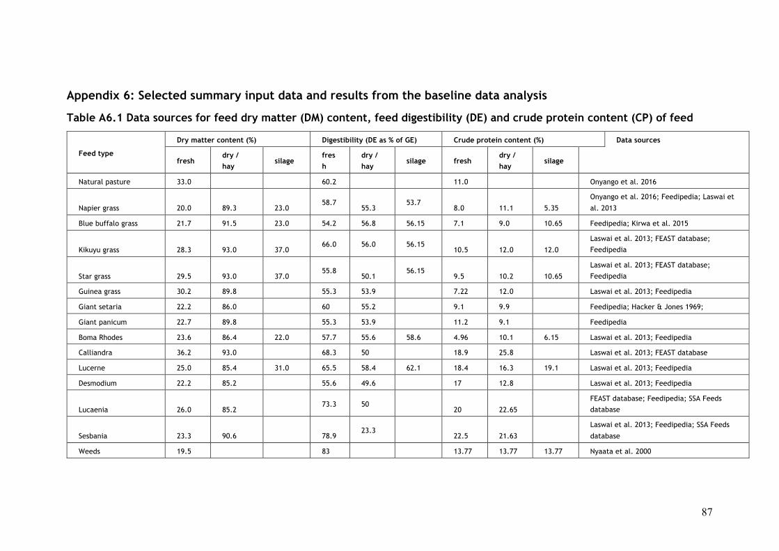
87

Appendix 6: Selected summary input data and results from the baseline data analysis

Table A6.1 Data sources for feed dry matter (DM) content, feed digestibility (DE) and crude protein content (CP) of feed

Feed type

Dry matter content (%) Digestibility (DE as % of GE) Crude protein content (%) Data sources

fresh dry /

hay silage

fres

h

dry /

hay silage fresh

dry /

hay silage

Natural pasture 33.0 60.2 11.0 Onyango et al. 2016

Napier grass 20.0 89.3 23.0 58.7

55.3 53.7

8.0 11.1 5.35

Onyango et al. 2016; Feedipedia; Laswai et

al. 2013

Blue buffalo grass 21.7 91.5 23.0 54.2 56.8 56.15 7.1 9.0 10.65 Feedipedia; Kirwa et al. 2015

Kikuyu grass 28.3 93.0 37.0 66.0 56.0 56.15

10.5 12.0 12.0

Laswai et al. 2013; FEAST database;

Feedipedia

Star grass 29.5 93.0 37.0 55.8

50.1 56.15

9.5 10.2 10.65

Laswai et al. 2013; FEAST database;

Feedipedia

Guinea grass 30.2 89.8 55.3 53.9 7.22 12.0 Laswai et al. 2013; Feedipedia

Giant setaria 22.2 86.0 60 55.2 9.1 9.9 Feedipedia; Hacker & Jones 1969;

Giant panicum 22.7 89.8 55.3 53.9 11.2 9.1 Feedipedia

Boma Rhodes 23.6 86.4 22.0 57.7 55.6 58.6 4.96 10.1 6.15 Laswai et al. 2013; Feedipedia

Calliandra 36.2 93.0 68.3 50 18.9 25.8 Laswai et al. 2013; FEAST database

Lucerne 25.0 85.4 31.0 65.5 58.4 62.1 18.4 16.3 19.1 Laswai et al. 2013; Feedipedia

Desmodium 22.2 85.2 55.6 49.6 17 12.8 Laswai et al. 2013; Feedipedia

Lucaenia 26.0 85.2 73.3 50

20 22.65

FEAST database; Feedipedia; SSA Feeds

database

Sesbania 23.3 90.6 78.9 23.3

22.5 21.63

Laswai et al. 2013; Feedipedia; SSA Feeds

database

Weeds 19.5 83 13.77 13.77 13.77 Nyaata et al. 2000

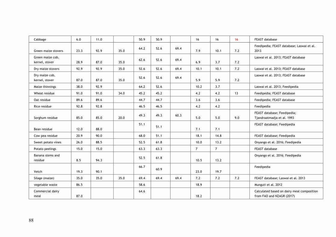
88

Cabbage 6.0 11.0 50.9 50.9 16 16 16 FEAST database

Green maize stovers 23.3 92.9 35.0 64.2 52.6 69.4

7.9 10.1 7.2

Feedipedia; FEAST database; Laswai et al.

2013

Green maize cob,

kernel, stover 28.9 87.0 35.0 62.6 52.6 69.4

6.9 3.7 7.2

Laswai et al. 2013; FEAST database

Dry maize stovers 92.9 92.9 35.0 52.6 52.6 69.4 10.1 10.1 7.2 Laswai et al. 2013; FEAST database

Dry maize cob,

kernel, stover 87.0 87.0 35.0 52.6 52.6 69.4

5.9 5.9 7.2

Laswai et al. 2013; FEAST database

Maize thinnings 38.0 92.9 64.2 52.6 10.2 3.7 Laswai et al. 2013; Feedipedia

Wheat residue 91.0 91.0 34.0 45.2 45.2 4.2 4.2 13 Feedipedia; FEAST database

Oat residue 89.6 89.6 44.7 44.7 3.6 3.6 Feedipedia; FEAST database

Rice residue 92.8 92.8 46.5 46.5 4.2 4.2 Feedipedia

Sorghum residue 85.0 85.0 20.0 49.3 49.3 60.3

5.0 5.0 9.0

FEAST database; Feedipedia;

Tjandraatmadja et al. 1993

Bean residue 12.0 88.0

51.1

51.1

7.1 7.1

FEAST database; Feedipedia

Cow pea residue 20.9 90.0 68.0 51.1 18.1 14.8 FEAST database; Feedipedia

Sweet potato vines 26.0 88.5 52.5 61.8 10.0 13.2 Onyango et al. 2016; Feedipedia

Potato peelings 15.0 15.0 63.3 63.3 7 7 FEAST database

Banana stems and

residue 8.5 94.3 52.5 61.8

10.5 13.2

Onyango et al. 2016; Feedipedia

Vetch 19.3 90.1

66.7

60.9

23.0 19.7

Feedipedia

Silage (maize) 35.0 35.0 35.0 69.4 69.4 69.4 7.2 7.2 7.2 FEAST database; Laswai et al. 2013

vegetable waste 86.5 58.6 18.9 Munguti et al. 2012

Commercial dairy

meal 87.0

64.6

18.2

Calculated based on dairy meal composition

from FAO and NZAGR (2017)

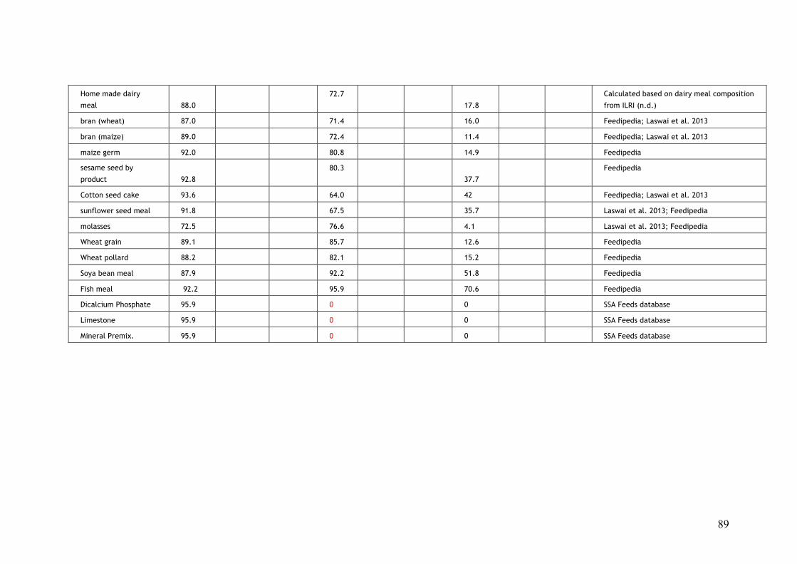
89

Home made dairy

meal 88.0

72.7

17.8

Calculated based on dairy meal composition

from ILRI (n.d.)

bran (wheat) 87.0 71.4 16.0 Feedipedia; Laswai et al. 2013

bran (maize) 89.0 72.4 11.4 Feedipedia; Laswai et al. 2013

maize germ 92.0 80.8 14.9 Feedipedia

sesame seed by

product 92.8

80.3

37.7

Feedipedia

Cotton seed cake 93.6 64.0 42 Feedipedia; Laswai et al. 2013

sunflower seed meal 91.8 67.5 35.7 Laswai et al. 2013; Feedipedia

molasses 72.5 76.6 4.1 Laswai et al. 2013; Feedipedia

Wheat grain 89.1 85.7 12.6 Feedipedia

Wheat pollard 88.2 82.1 15.2 Feedipedia

Soya bean meal 87.9 92.2 51.8 Feedipedia

Fish meal 92.2 95.9 70.6 Feedipedia

Dicalcium Phosphate 95.9 0 0 SSA Feeds database

Limestone 95.9 0 0 SSA Feeds database

Mineral Premix. 95.9 0 0 SSA Feeds database

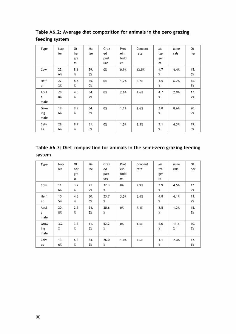
90

Table A6.2: Average diet composition for animals in the zero grazing feeding system

Type Nap

ier

Ot

her

gra

ss

Ma

ize

Graz

ed

past

ure

Prot

ein

fodd

er

Concent

rate

Ma

ize

ger

m

Mine

rals

Ot

her

Cow 22.

6%

8.6

%

29.

3% 0% 0.9% 13.5% 4.7

% 4.4% 15.

6%

Heif

er

22.

3%

8.8

%

35.

0% 0% 1.2% 6.7% 3.5

% 6.2% 16.

3%

Adul

t

male

28.

8%

4.5

%

34.

7%

0% 2.6% 4.6% 4.7

%

2.9% 17.

2%

Grow

ing

male

19.

6%

9.9

%

34.

5% 0% 1.1% 2.6% 2.8

% 8.6% 20.

9%

Calv

es

28.

6%

8.7

%

31.

8% 0% 1.5% 3.3% 2.1

% 4.3% 19.

8%

Table A6.3: Diet composition for animals in the semi-zero grazing feeding system

Type Nap

ier

Ot

her

gra

ss

Ma

ize

Graz

ed

past

ure

Prot

ein

fodd

er

Concent

rate

Ma

ize

ger

m

Mine

rals

Ot

her

Cow 11.

6%

3.7

%

21.

9%

32.3

% 0% 9.9% 2.9

% 4.5% 12.

9%

Heif

er

10.

5%

4.3

%

30.

6%

23.7

%

3.5% 5.4% 4.8

%

4.1% 13.

2%

Adul

t

male

20.

8%

2.5

%

24.

5%

30.6

%

0% 2.1% 2.5

%

1.2% 15.

9%

Grow

ing

male

3.2

%

3.3

%

11.

5%

52.2

% 0% 1.6% 6.0

%

11.6

%

10.

7%

Calv

es

13.

6%

6.3

%

34.

5%

26.0

% 1.0% 2.6% 1.1

% 2.4% 12.

6%

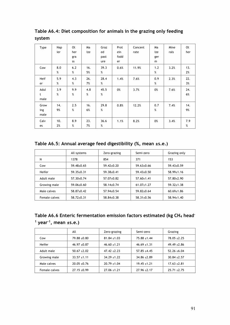
91

Table A6.4: Diet composition for animals in the grazing only feeding system

Type Nap

ier

Ot

her

gra

ss

Ma

ize

Graz

ed

past

ure

Prot

ein

fodd

er

Concent

rate

Ma

ize

ger

m

Mine

rals

Ot

her

Cow 8.0

%

6.2

%

16.

5%

39.3

% 0.6% 11.9% 1.2

% 3.2% 13.

2%

Heif

er

5.9

%

4.3

%

26.

7%

28.4

% 1.4% 7.6% 0.9

% 2.3% 22.

3%

Adul

t

male

3.9

%

9.9

%

4.8

%

45.5

%

0% 3.7% 0% 7.6% 24.

6%

Grow

ing

male

14.

9%

2.5

%

16.

6%

29.8

% 0.8% 12.2% 0.7

% 7.4% 14.

9%

Calv

es

10.

2%

8.9

%

23.

7%

36.6

% 1.1% 8.2% 0% 3.4% 7.9

%

Table A6.5: Annual average feed digestibility (%, mean ±s.e.)

All systems Zero-grazing Semi-zero Grazing only

N 1378 854 371 153

Cow 59.48±0.65 59.42±0.20 59.63±0.66 59.43±0.59

Heifer 59.35±0.31 59.38±0.41 59.43±0.50 58.99±1.16

Adult male 57.30±0.74 57.07±0.82 57.60±1.41 57.80±2.90

Growing male 59.06±0.60 58.14±0.74 61.07±1.27 59.32±1.38

Male calves 58.87±0.42 57.94±0.54 59.82±0.64 60.69±1.86

Female calves 58.72±0.31 58.84±0.38 58.31±0.56 58.94±1.40

Table A6.6 Enteric fermentation emission factors estimated (kg CH4 head-

1 year-1, mean ±s.e.)

All Zero-grazing Semi-zero Grazing

Cow 79.88 ±0.80 81.84 ±1.03 75.88 ±1.44 78.05 ±2.25

Heifer 46.97 ±0.87 46.60 ±1.21 46.69 ±1.31 49.49 ±2.86

Adult male 50.67 ±2.02 47.42 ±2.23 57.85 ±4.45 52.26 ±6.04

Growing male 33.57 ±1.11 34.29 ±1.22 34.86 ±2.89 30.84 ±2.57

Male calves 20.05 ±0.76 20.79 ±1.04 19.45 ±1.21 17.63 ±2.81

Female calves 27.15 ±0.99 27.06 ±1.21 27.96 ±2.17 25.71 ±2.75

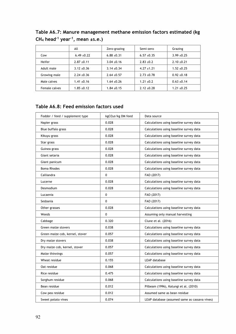
92

Table A6.7: Manure management methane emission factors estimated (kg CH4 head-1 year-1, mean ±s.e.)

All Zero-grazing Semi-zero Grazing

Cow 6.49 ±0.22 6.88 ±0.31 6.57 ±0.35 3.99 ±0.25

Heifer 2.87 ±0.11 3.04 ±0.16 2.83 ±0.2 2.10 ±0.21

Adult male 3.12 ±0.36 3.14 ±0.34 4.27 ±1.21 1.52 ±0.25

Growing male 2.24 ±0.36 2.64 ±0.57 2.73 ±0.78 0.92 ±0.18

Male calves 1.41 ±0.16 1.64 ±0.26 1.21 ±0.2 0.63 ±0.14

Female calves 1.85 ±0.12 1.84 ±0.15 2.12 ±0.28 1.21 ±0.25

Table A6.8: Feed emission factors used

Fodder / feed / supplement type kgCO2e/kg DM feed Data source

Napier grass 0.028 Calculations using baseline survey data

Blue buffalo grass 0.028 Calculations using baseline survey data

Kikuyu grass 0.028 Calculations using baseline survey data

Star grass 0.028 Calculations using baseline survey data

Guinea grass 0.028 Calculations using baseline survey data

Giant setaria 0.028 Calculations using baseline survey data

Giant panicum 0.028 Calculations using baseline survey data

Boma Rhodes 0.028 Calculations using baseline survey data

Calliandra 0 FAO (2017)

Lucerne 0.028 Calculations using baseline survey data

Desmodium 0.028 Calculations using baseline survey data

Lucaenia 0 FAO (2017)

Sesbania 0 FAO (2017)

Other grasses 0.028 Calculations using baseline survey data

Weeds 0 Assuming only manual harvesting

Cabbage 0.320 Clune et al. (2016)

Green maize stovers 0.038 Calculations using baseline survey data

Green maize cob, kernel, stover 0.057 Calculations using baseline survey data

Dry maize stovers 0.038 Calculations using baseline survey data

Dry maize cob, kernel, stover 0.057 Calculations using baseline survey data

Maize thinnings 0.057 Calculations using baseline survey data

Wheat residue 0.155 LEAP database

Oat residue 0.068 Calculations using baseline survey data

Rice residue 0.475 Calculations using baseline survey data

Sorghum residue 0.068 Calculations using baseline survey data

Bean residue 0.012 Pilbeam (1996), Katungi et al. (2010)

Cow pea residue 0.012 Assumed same as bean residue

Sweet potato vines 0.074 LEAP database (assumed same as cassava vines)

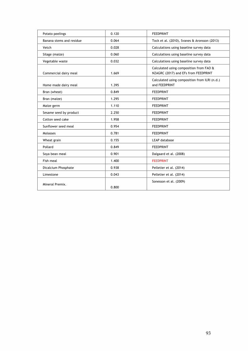
93

Potato peelings 0.120 FEEDPRINT

Banana stems and residue 0.064 Tock et al. (2010), Svanes & Aronsson (2013)

Vetch 0.028 Calculations using baseline survey data

Silage (maize) 0.060 Calculations using baseline survey data

Vegetable waste 0.032 Calculations using baseline survey data

Commercial dairy meal 1.669

Calculated using composition from FAO &

NZAGRC (2017) and EFs from FEEDPRINT

Home made dairy meal 1.395

Calculated using composition from ILRI (n.d.)

and FEEDPRINT

Bran (wheat) 0.849 FEEDPRINT

Bran (maize) 1.295 FEEDPRINT

Maize germ 1.110 FEEDPRINT

Sesame seed by product 2.250 FEEDPRINT

Cotton seed cake 1.958 FEEDPRINT

Sunflower seed meal 0.954 FEEDPRINT

Molasses 0.781 FEEDPRINT

Wheat grain 0.155 LEAP database

Pollard 0.849 FEEDPRINT

Soya bean meal 0.901 Dalgaard et al. (2008)

Fish meal 1.400 FEEDPRINT

Dicalcium Phosphate 0.938 Pelletier et al. (2014)

Limestone 0.043 Pelletier et al. (2014)

Mineral Premix. 0.800

Sonesson et al. (2009)

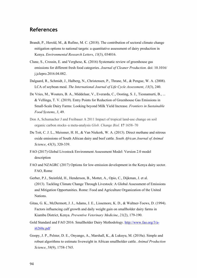
94

References

Brandt, P., Herold, M., & Rufino, M. C. (2018). The contribution of sectoral climate change

mitigation options to national targets: a quantitative assessment of dairy production in

Kenya. Environmental Research Letters, 13(3), 034016.

Clune, S., Crossin, E. and Verghese, K. (2016) Systematic review of greenhouse gas

emissions for different fresh food categories. Journal of Cleaner Production. doi: 10.1016/

j.jclepro.2016.04.082.

Dalgaard, R., Schmidt, J., Halberg, N., Christensen, P., Thrane, M., & Pengue, W. A. (2008).

LCA of soybean meal. The International Journal of Life Cycle Assessment, 13(3), 240.

De Vries, M., Wouters, B. A., Middelaar, V., Everarda, C., Oosting, S. J., Tiesnamurti, B., ...

& Vellinga, T. V. (2019). Entry Points for Reduction of Greenhouse Gas Emissions in

Small-Scale Dairy Farms: Looking beyond Milk Yield Increase. Frontiers in Sustainable Food Systems, 3, 49.

Don A, Schumacher J and Freibauer A 2011 Impact of tropical land-use change on soil

organic carbon stocks–a meta-analysis Glob. Change Biol. 17 1658–70

Du Toit, C. J. L., Meissner, H. H., & Van Niekerk, W. A. (2013). Direct methane and nitrous

oxide emissions of South African dairy and beef cattle. South African Journal of Animal Science, 43(3), 320-339.

FAO (2017) Global Livestock Environment Assessment Model: Version 2.0 model

description

FAO and NZAGRC (2017) Options for low-emission development in the Kenya dairy sector.

FAO, Rome

Gerber, P.J., Steinfeld, H., Henderson, B., Mottet, A., Opio, C., Dijkman, J. et al.

(2013). Tackling Climate Change Through Livestock: A Global Assessment of Emissions

and Mitigation Opportunities. Rome: Food and Agriculture Organization of the United

Nations.

Gitau, G. K., McDermott, J. J., Adams, J. E., Lissemore, K. D., & Waltner-Toews, D. (1994).

Factors influencing calf growth and daily weight gain on smallholder dairy farms in

Kiambu District, Kenya. Preventive Veterinary Medicine, 21(2), 179-190.

Gold Standard and FAO 2016. Smallholder Dairy Methodology. http://www.fao.org/3/a-

i6260e.pdf

Goopy, J. P., Pelster, D. E., Onyango, A., Marshall, K., & Lukuyu, M. (2018a). Simple and

robust algorithms to estimate liveweight in African smallholder cattle. Animal Production Science, 58(9), 1758-1765.

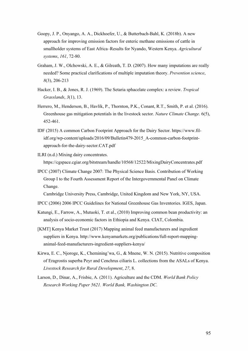
95

Goopy, J. P., Onyango, A. A., Dickhoefer, U., & Butterbach-Bahl, K. (2018b). A new

approach for improving emission factors for enteric methane emissions of cattle in

smallholder systems of East Africa–Results for Nyando, Western Kenya. Agricultural systems, 161, 72-80.

Graham, J. W., Olchowski, A. E., & Gilreath, T. D. (2007). How many imputations are really

needed? Some practical clarifications of multiple imputation theory. Prevention science,

8(3), 206-213

Hacker, I. B., & Jones, R. J. (1969). The Setaria sphacelate complex: a review. Tropical Grasslands, 3(1), 13.

Herrero, M., Henderson, B., Havlík, P., Thornton, P.K., Conant, R.T., Smith, P. et al. (2016).

Greenhouse gas mitigation potentials in the livestock sector. Nature Climate Change. 6(5),

452-461.

IDF (2015) A common Carbon Footprint Approach for the Dairy Sector. https://www.fil-

idf.org/wp-content/uploads/2016/09/Bulletin479-2015_A-common-carbon-footprint-

approach-for-the-dairy-sector.CAT.pdf

ILRI (n.d.) Mixing dairy concentrates.

https://cgspace.cgiar.org/bitstream/handle/10568/12522/MixingDairyConcentrates.pdf

IPCC (2007) Climate Change 2007: The Physical Science Basis. Contribution of Working

Group I to the Fourth Assessment Report of the Intergovernmental Panel on Climate

Change.

Cambridge University Press, Cambridge, United Kingdom and New York, NY, USA.

IPCC (2006) 2006 IPCC Guidelines for National Greenhouse Gas Inventories. IGES, Japan.

Katungi, E., Farrow, A., Mutuoki, T. et al., (2010) Improving common bean productivity: an

analysis of socio-economic factors in Ethiopia and Kenya. CIAT, Colombia.

[KMT] Kenya Market Trust (2017) Mapping animal feed manufacturers and ingredient

suppliers in Kenya. http://www.kenyamarkets.org/publications/full-report-mapping-

animal-feed-manufacturers-ingredient-suppliers-kenya/

Kirwa, E. C., Njoroge, K., Chemining’wa, G., & Mnene, W. N. (2015). Nutritive composition

of Eragrostis superba Peyr and Cenchrus ciliaris L. collections from the ASALs of Kenya.

Livestock Research for Rural Development, 27, 8.

Larson, D., Dinar, A., Frisbie, A. (2011). Agriculture and the CDM. World Bank Policy Research Working Paper 5621. World Bank, Washington DC.

96

Laswai, G.H., Mgheni, D.M., Mtenga, L.A., Ndikumana, J., Zziwa, E. (Eds), 2013. Chemical

Composition and Nutritional Values of Feed Resources for Ruminants: Eastern and Central

Africa (ECA) Feedstuff Table for Ruminants. ASARECA, Entebbe.

LEAP database. http://www.fao.org/partnerships/leap/database/ghg-crops/en/

Lukuyu, B., Franzel, S., Ongadi, P. M., & Duncan, A. J. (2011). Livestock feed resources:

Current production and management practices in central and northern rift valley provinces

of Kenya. Livestock Research for Rural Development, 23(5), 112.

Methu, J. N., Owen, E., Abate, A. L., & Tanner, J. C. (2001). Botanical and nutritional

composition of maize stover, intakes and feed selection by dairy cattle. Livestock Production Science, 71(2-3), 87-96.

Mottet, A., Henderson, B., Opio, C., Falcucci, A., Tempio, G, Silvestry, S. et al. (2017).

Climate change mitigation and productivity gains in livestock supply chains: insights

from regional case studies. Regional Environmental Change. 17:129.

doi.org/10.1007/s10113-016-0986-3

Munguti, J., Charo-Karisa, H., Opiyo, M. A., Ogello, E. O., Marijani, E., Nzayisenga, L., &

Liti, D. (2012). Nutritive value and availability of commonly used feed ingredients for

farmed Nile tilapia (Oreochromis niloticus L.) and African catfish (Clarias gariepinus,

Burchell) in Kenya, Rwanda and Tanzania. African Journal of Food, Agriculture, Nutrition and Development, 12(3), 6135-6155.

Nafula, S. S. (2013). The impact of enhanced nutritional and feeding practices on growth and health of dairy calves in Mukurweini district of Kenya. Doctoral dissertation, University of

Nairobi.

Ndung’u, P. W., Bebe, B. O., Ondiek, J. O., Butterbach-Bahl, K., Merbold, L., & Goopy, J. P.

(2019). Improved region-specific emission factors for enteric methane emissions from

cattle in smallholder mixed crop: livestock systems of Nandi County, Kenya. Animal Production Science, 59(6), 1136-1146.

NRC (1996) Nutrient Requirements of Beef Cattle. National Academies Press.

NRC (2001) Nutrient Requirements of Dairy Cattle. National Academies Press.

Nyaata, O. Z., Dorward, P. T., Keatinge, J. D. H., & O'neill, M. K. (2000). Availability and

use of dry season feed resources on smallholder dairy farms in central Kenya. Agroforestry Systems, 50(3), 315-331.

Onyango, A., Dickhoefer, U., Butterbach-Bahl, K. and Goopy, J. (2016). Digestibility and

metabolizable energy of selected tropical feedstuffs estimated by in vitro and prediction

equations. Poster presented at Tropentag 2016.

97

Opio, C., Gerber, P., Mottet, A., Falcucci, A., Tempio, G., MacLeod, M., Vellinga, T.,

Henderson, B. and Steinfeld, H. 2013. Greenhouse gas emissions from ruminant supply chains – A global life cycle assessment. Food and Agriculture Organization of the United

Nations (FAO), Rome.

Pelletier, N., Ibarburu, M., & Xin, H. (2014). Comparison of the environmental footprint of

the egg industry in the United States in 1960 and 2010. Poultry science, 93(2), 241-255.

Pilbeam, C. J. (1996). Variation in harvest index of maize (Zea mays) and common bean

(Phaseolus vulgaris) grown in a marginal rainfall area of Kenya. The Journal of Agricultural Science, 126(1), 1-6.

Saatchi, S. S., Harris, N. L., Brown, S., Lefsky, M., Mitchard, E. T., Salas, W., ... & Petrova,

S. (2011). Benchmark map of forest carbon stocks in tropical regions across three

continents. Proceedings of the national academy of sciences, 108(24), 9899-9904.

Safley, L. M. (1992). Global methane emissions from livestock and poultry manure. United

States Environmental Protection Agency.

Smith, P., Clark, H., Dong, H., Elsiddig, E.A., Haberl, H., Harper, R. et al. (2014). Chapter 11: Agriculture, forestry and other land use (AFOLU). In Climate Change 2014:

Mitigation of Climate Change. IPCC Working Group III Contribution to AR5, ed.

Edenhofer, O., Pichs-Madruga, R., Sokona, Y., Minx, J.C., Farahani, E., Kadner, S.,

Seyboth, K., Adler, A., Baum, I., Brunner, S., Eickemeier, P., Kriemann, B., Savolainen,

J., Schlömer, S., von Stechow, C. and Zwickel, T. (Cambridge: Cambridge University

Press), 811-922.

Sonesson, U., Cederberg, C. and M. Berglund (2009) Greenhouse gas emissions in animal

feed production: decision support for certification. http://www.klimatmarkningen.se/wp-

content/uploads/2009/12/2009-2-feed.pdf

Spalding-Fecher, R., & Michaelowa, A. (2013). Should the use of standardized baselines in

the CDM be mandatory?. Climate policy, 13(1), 80-88.

Staal, S. J., Baltenweck, I., Waithaka, M. M., DeWolff, T., & Njoroge, L. (2002). Location

and uptake: integrated household and GIS analysis of technology adoption and land use,

with application to smallholder dairy farms in Kenya. Agricultural Economics, 27(3), 295-

315.

State Department of Livestock (2017). Dairy NAMA concept note.

http://www.kilimo.go.ke/wp-content/uploads/2018/03/NAMA-Kenya-Dairy-NAMA-GCF-

concept-NoteJanuary-2017-1.pdf

State Department of Livestock (2019) Inventory of GHG emissions from dairy cattle in Kenya

(1995-2017). Unpublished document.

98

Svanes, E., & Aronsson, A. K. (2013). Carbon footprint of a Cavendish banana supply chain.

The International Journal of Life Cycle Assessment, 18(8), 1450-1464.

Tjandraatmadja, M., MacRae, I. C., & Norton, B. W. (1993). Intake and digestibility of

sorghum silage by goats. Animal feed science and technology, 41(3), 171-179.

Tock, J. Y., Lai, C. L., Lee, K. T., Tan, K. T., & Bhatia, S. (2010). Banana biomass as

potential renewable energy resource: A Malaysian case study. Renewable and sustainable energy reviews, 14(2), 798-805.

Tubiello, F.N., Salvatore, M., Condor-Golec R.D., Ferrara, A., Rossi, S., Biancalani, R. et al.

(2014). Agriculture, Forestry and Other Land Use Emissions by Sources and Removals by

Sinks, 1990-2011 Analysis. Rome: Food and Agriculture Organization of the United

Nations.

[UN DESA] UN Department for Social and Economic Affairs (2005) Designing Household

Survey Samples.

https://unstats.un.org/unsd/demographic/sources/surveys/Handbook23June05.pdf

Weiler, V., Udo, H. M., Viets, T., Crane, T. A., & De Boer, I. J. (2014). Handling multi-

functionality of livestock in a life cycle assessment: the case of smallholder dairying in

Kenya. Current Opinion in Environmental Sustainability, 8, 29-38.

Wilkes, A., Reisinger, A., Wollenberg, E. K., & Dijk, S. V. (2017). Measurement, reporting

and verification of livestock GHG emissions by developing countries in the UNFCCC:

current practices and opportunities for improvement.

Wilkes, A., Rosenstock, T. S., Namoi, N., and Fraval, S. (2018). Suitability of project M&E

systems to support agricultural MRV: The case of the Kenya dairy NAMA. CCAFS

working paper.

Wood, S. and A. Cowie 2004. A review of greenhouse gas emission factors for fertilizer production. Cooperative Research Centre for Greenhouse Accounting.

World Bank and FAO (2019) Investing in Sustainable Livestock Guide.

https://www.sustainablelivestockguide.org/

Zezza, A., Federighi, G., Kalilou, A. A. and Hiernaux, P. (2016). Milking the data: Measuring

milk off-take in extensive livestock systems. Experimental evidence from Niger. Food policy, 59, 174-186.

The CGIAR Research Program on Climate Change, Agriculture and Food

Security (CCAFS) brings together some of the world’s best researchers

in agricultural science, development research, climate science and Earth

system science, to identify and address the most important interactions,

synergies and tradeoffs between climate change, agriculture and food

security. For more information, visit us at https://ccafs.cgiar.org/.

Titles in this series aim to disseminate interim climate change,

agriculture and food security research and practices and stimulate

feedback from the scientific community.

CCAFS research is supported by:

CCAFS is led by:

Science for a food-secure future

Documents

Methods and guidance to support MRV of livestock emissions dairy... · 2019-11-18 · Methods and guidance to support MRV of livestock emissions Methods for data collection, analysis