Method of Moments (MoM): Application for

Solving Augmented Electric Field Integral Equation (AEFIE)

By

Binye Li

Senior  Thesis  in  Electrical  Engineering  

University  of  Illinois  at  Urbana-­‐Champaign  

Advisor:  Weng  Cho  Chew  

 

 

 

December 2014

ii    

Abstract

Surface integral equations (SIEs) are promising candidates for modeling circuits because they

reduce degrees of freedom by restricting physical unknowns on the surface, which simplifies

complex structures. However, there are still challenges related to achieving stability over a broad

frequency band. Specifically, the low frequency breakdown of electrical field integral equation

(EFIE) operator is discussed in this work. In order to solve or alleviate this problem, the

separation of irrotational and solenoidal current must be accomplished. A proposed method, the

Augmented Electrical Field Integral Equation (AEFIE), is intended to separate the current

element by introducing charge as another variable and relate irrotational current and the charge

vector. Finally, the method of moments (MoM) is applied to solve the integral equation by

projecting the current onto RWG basis and performing subspace projections to fill out the

integral equation operator matrix. For complicated circuit structure, MoM can be accelerated

using the fast multipole algorithm (FMA).

Subject  Keywords:  ECE  499;  Senior  Thesis;  Computational  Electromagnetics;  EFIE;  MoM

iii    

Table of Contents

1. Introduction………………………………………….………………………………….. 1

2. Introduction to Electric Field Integral Equation (EFIE)………………………………... 2

3. Low Frequency Breakdown with EFIE…………………..…………………………….. 9

4. Formulation of Augmented Electric Field Integral Equation (AEFIE)……….……....... 15

5. Method of Moment (MoM) in A-EFIE………………………………………………..... 20

6. Design of Graphical User Interface………………………………...………………….... 22

7. Conclusion……………………………………………………………………………..... 25

References…………………………………………………………………………………… 26

Appendix A： Source code of GUI........................................................................................ 27

  1  

1. Introduction

The design of microelectronic devices is faced with many challenges, such as signal integrity,

power integrity, electromagnetic interference, and so on. It is also not practical to put design into

production before investigating the potential problems of such design. In order to know the flaws

of a design beforehand, computational electromagnetics is the research area that provides

accurate simulation result. Unlike traditional quasi-static methods, which neglects displacement

current and focus on the problem in low frequency. Surface Integral Equation (SIE) method is

going to give full wave electromagnetic analysis [3]. This project is going to focus on the

challenges associated with this method and potential solutions.

  2  

2. Introduction to Electric Field Integral Equation (EFIE)

2.1 Electrical Field Wave Equation

It will be most intuitive to introduce Maxwell’s equations before studying electromagnetic

problems. The differential form of Maxwell’s equations can be written as

∇× E = iωµH (2.1)

∇× H = −iωεE + J (2.2)

∇⋅εE = ρe (2.3)

∇⋅µH = 0 (2.4)

In homogeneous media, the wave equation for the electrical field can be derived by taking the

curl of Faraday’s Law,

∇×∇× E = iωµ∇× H (2.5)

and substituting with Ampere’s Law,

∇×∇× E = iωµ(−iωεE + J) =ω 2µεE + iωµJ (2.6)

k2 =ω 2µε (2.7)

As for homogeneous medium, the wave number is a constant. The wave equation of an electrical

field with spatial dependence r is

∇×∇× E(r)− k2E(r) = iωµJ(r) (2.8)

  3  

2.2 The Dyadic Green’s Function

The dyadic Green’s function is the point source response to the vector wave equation [1]. The

electric field can be formulized alternatively with the dyadic Green’s function

E(r) = iωµ dr 'V∫ J(r ' ) ⋅G

_(r ' , r) (2.9)

Applying equation (2.9) to the wave equation derived in the last section, the following equation

is achieved:

∇×∇×G_(r)− k2G

_(r) = I

_δ (r - r ' ) (2.10)

The right-hand side of this equation represents the point source. Mathematically, the solution [1]

is given by

G_(r) = (I

_+ ∇∇k2) eik r−r '

4π r − r ' (2.11)

Once the point source is known, the solution to the corresponding dyadic Green’s function can be

achieved by equation (2.11) [1]. Theoretically, the resulting electrical field distribution can be

calculated when the current distribution and the point source response are given. In the next

section, the equivalence principle is introduced to come up with the surface integral, and thus the

electrical field integral equation (EFIE).

  4  

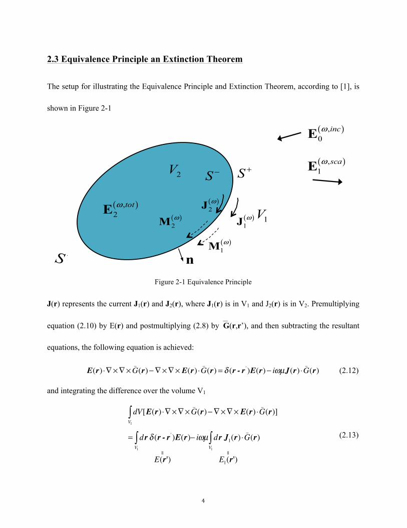
2.3 Equivalence Principle an Extinction Theorem

The setup for illustrating the Equivalence Principle and Extinction Theorem, according to [1], is

shown in Figure 2-1

Figure 2-1 Equivalence Principle

J(r) represents the current J1(r) and J2(r), where J1(r) is in V1 and J2(r) is in V2. Premultiplying

equation (2.10) by E(r) and postmultiplying (2.8) by�G(r,r’), and then subtracting the resultant

equations, the following equation is achieved:

E(r) ⋅∇ ×∇×G_(r)−∇×∇× E(r) ⋅G

_(r) = δ (r - r ' )E(r)− iωµJ(r) ⋅G

_(r) (2.12)

and integrating the difference over the volume V1

dV[E(r) ⋅∇ ×∇×G_(r)−∇×∇× E(r) ⋅G

_(r)

V1∫ ]

= dr δ (r - r ' )E(r)V1∫

E(r')||

− iωµ dr J1(r) ⋅G_(r)

V1∫

E1(r')||

(2.13)

S +

( ),0incωE

( ),1scaωE

 

S +S −

   

   

( ),2totωE

( )1ωJ

( )1ωM

( )2ωM

( )2ωJ

1V

2V

n

  5  

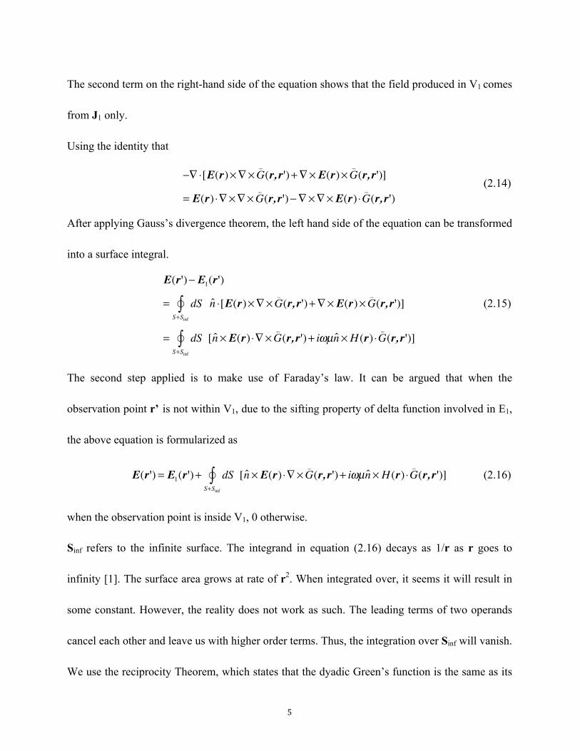
The second term on the right-hand side of the equation shows that the field produced in V1 comes

from J1 only.

Using the identity that

−∇⋅[E(r)×∇×G

_(r, r')+∇× E(r)×G

_(r, r')]

= E(r) ⋅∇ ×∇×G_(r, r')−∇×∇× E(r) ⋅G

_(r, r')

(2.14)

After applying Gauss’s divergence theorem, the left hand side of the equation can be transformed

into a surface integral.

E(r')− E1(r')

= dS n̂ ⋅[E(r)×∇×G_(r, r')+∇× E(r)×G

_(r, r')

S+Sinf!∫ ]

= dS [n̂ × E(r) ⋅∇ ×G_(r, r')+ iωµn̂ × H (r) ⋅G

_(r, r')

S+Sinf!∫ ]

(2.15)

The second step applied is to make use of Faraday’s law. It can be argued that when the

observation point r’ is not within V1, due to the sifting property of delta function involved in E1,

the above equation is formularized as

E(r') = E1(r')+ dS [n̂ × E(r) ⋅∇ ×G

_(r, r')+ iωµn̂ × H (r) ⋅G

_(r, r')

S+Sinf!∫ ] (2.16)

when the observation point is inside V1, 0 otherwise.

Sinf refers to the infinite surface. The integrand in equation (2.16) decays as 1/r as r goes to

infinity [1]. The surface area grows at rate of r2. When integrated over, it seems it will result in

some constant. However, the reality does not work as such. The leading terms of two operands

cancel each other and leave us with higher order terms. Thus, the integration over Sinf will vanish.

We use the reciprocity Theorem, which states that the dyadic Green’s function is the same as its

  6  

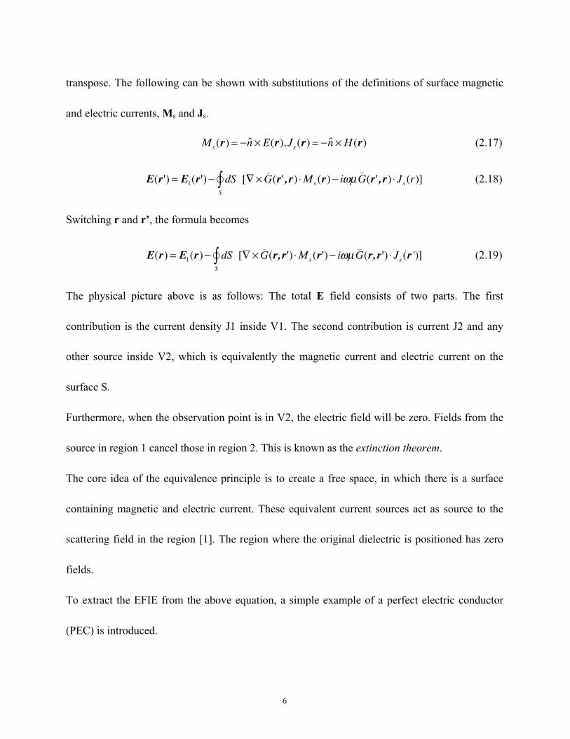
transpose. The following can be shown with substitutions of the definitions of surface magnetic

and electric currents, Ms and Js.

Ms (r) = −n̂ × E(r), Js (r) = −n̂ × H (r) (2.17)

E(r') = E1(r')− dS [∇×G

_(r', r) ⋅Ms (r)− iωµG

_(r', r) ⋅ Js (r)]

S!∫ (2.18)

Switching r and r’, the formula becomes

E(r) = E1(r)− dS [∇×G

_(r, r') ⋅Ms (r')− iωµG

_(r, r')

S!∫ ⋅ Js (r ')] (2.19)

The physical picture above is as follows: The total E field consists of two parts. The first

contribution is the current density J1 inside V1. The second contribution is current J2 and any

other source inside V2, which is equivalently the magnetic current and electric current on the

surface S.

Furthermore, when the observation point is in V2, the electric field will be zero. Fields from the

source in region 1 cancel those in region 2. This is known as the extinction theorem.

The core idea of the equivalence principle is to create a free space, in which there is a surface

containing magnetic and electric current. These equivalent current sources act as source to the

scattering field in the region [1]. The region where the original dielectric is positioned has zero

fields.

To extract the EFIE from the above equation, a simple example of a perfect electric conductor

(PEC) is introduced.

  7  

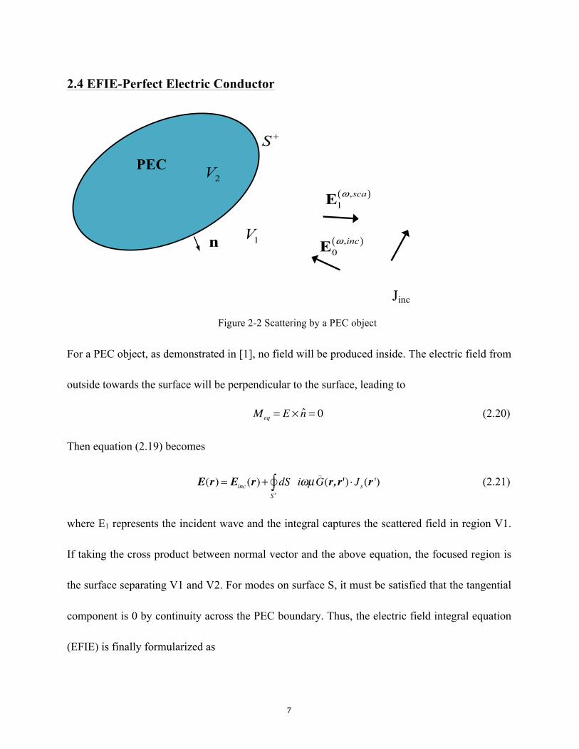
2.4 EFIE-Perfect Electric Conductor

Figure 2-2 Scattering by a PEC object

For a PEC object, as demonstrated in [1], no field will be produced inside. The electric field from

outside towards the surface will be perpendicular to the surface, leading to

Meq = E × n̂ = 0 (2.20)

Then equation (2.19) becomes

E(r) = Einc(r)+ dS iωµG

_(r, r') ⋅ Js (r ')

S+!∫ (2.21)

where E1 represents the incident wave and the integral captures the scattered field in region V1.

If taking the cross product between normal vector and the above equation, the focused region is

the surface separating V1 and V2. For modes on surface S, it must be satisfied that the tangential

component is 0 by continuity across the PEC boundary. Thus, the electric field integral equation

(EFIE) is finally formularized as

( ),0incωE

( ),1scaωE

 

S +

1V

2V

n

Jinc

PEC

  8  

E(r) = 0 = n̂ × Einc(r)+ iωµn̂ × dS ' G_(r, r')Jeq (r ')S∫ (2.22)

  9  

3. Low Frequency Breakdown of EFIE

3.1 Example of Low Frequency Breakdown

The electrical field integral equation is used to solve problems computationally, which results in

problems from the limited precision of computer.

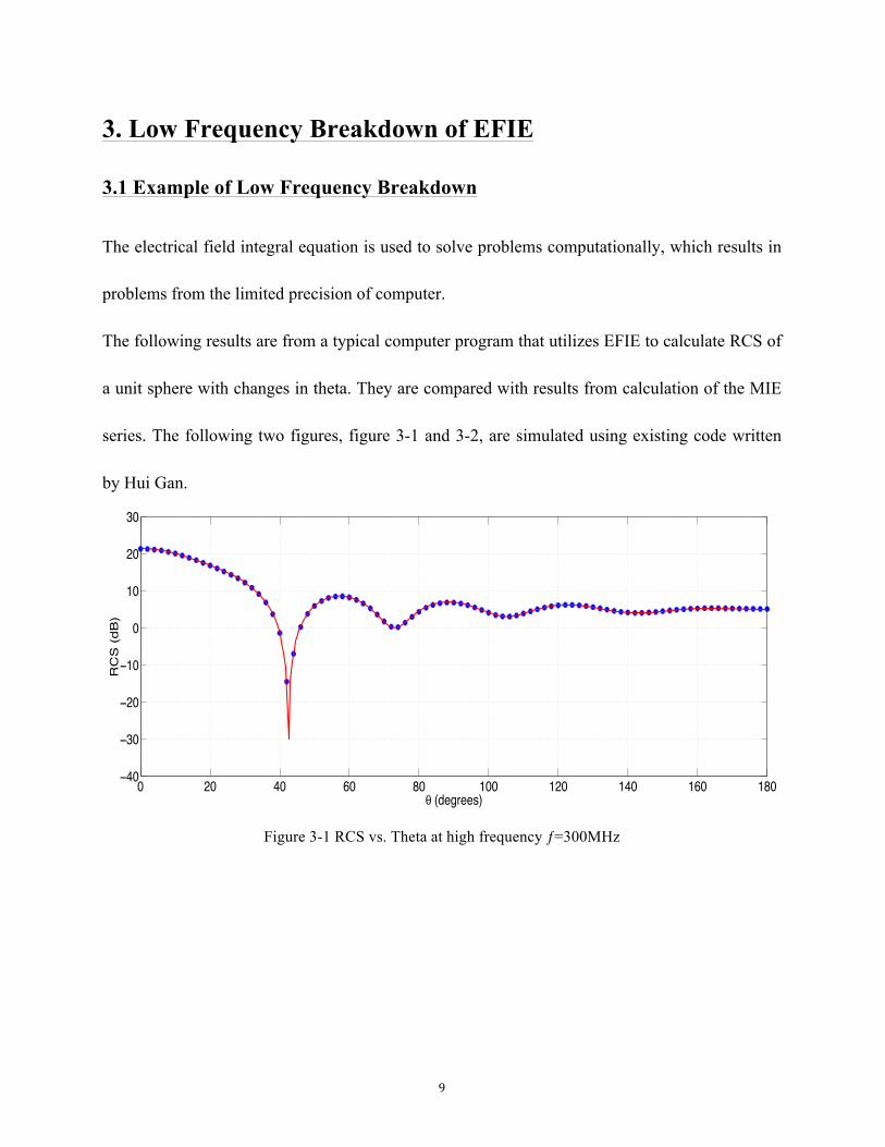
The following results are from a typical computer program that utilizes EFIE to calculate RCS of

a unit sphere with changes in theta. They are compared with results from calculation of the MIE

series. The following two figures, figure 3-1 and 3-2, are simulated using existing code written

by Hui Gan.

Figure 3-1 RCS vs. Theta at high frequency ƒ=300MHz

0 20 40 60 80 100 120 140 160 180−40

−30

−20

−10

0

10

20

30

θ (degrees)

RC

S (

dB)

  10  

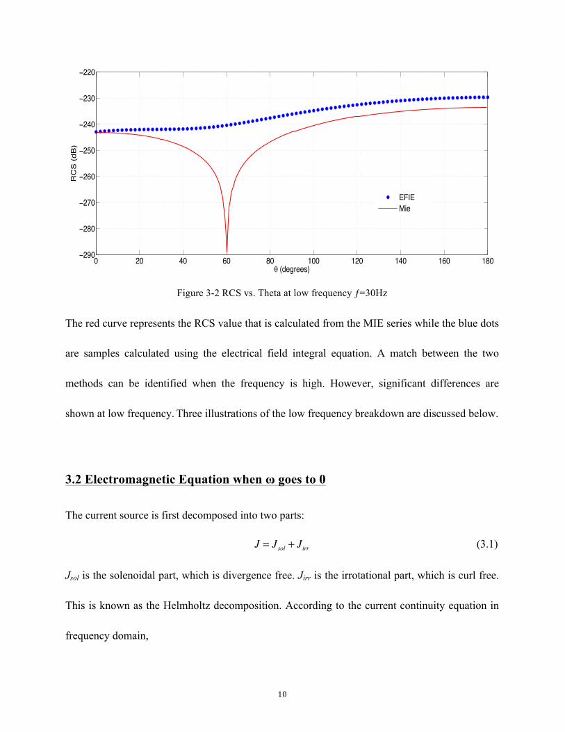
Figure 3-2 RCS vs. Theta at low frequency ƒ=30Hz

The red curve represents the RCS value that is calculated from the MIE series while the blue dots

are samples calculated using the electrical field integral equation. A match between the two

methods can be identified when the frequency is high. However, significant differences are

shown at low frequency. Three illustrations of the low frequency breakdown are discussed below.

3.2 Electromagnetic Equation when ω goes to 0

The current source is first decomposed into two parts:

J = Jsol + Jirr (3.1)

Jsol is the solenoidal part, which is divergence free. Jirr is the irrotational part, which is curl free.

This is known as the Helmholtz decomposition. According to the current continuity equation in

frequency domain,

0 20 40 60 80 100 120 140 160 180−290

−280

−270

−260

−250

−240

−230

−220

θ (degrees)

RC

S (

dB)

EFIEMie

  11  

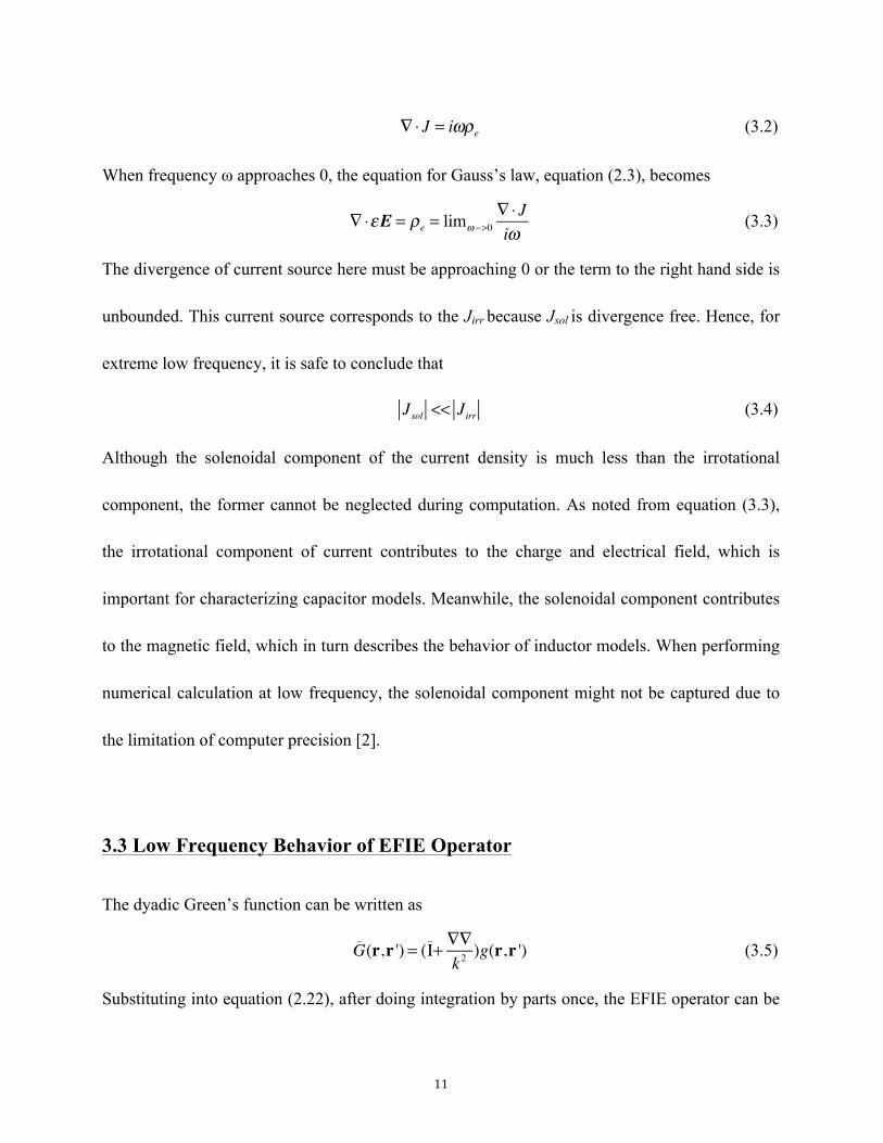
∇⋅ J = iωρe (3.2)

When frequency ω approaches 0, the equation for Gauss’s law, equation (2.3), becomes

∇⋅εE = ρe = limω −>0∇⋅ Jiω

(3.3)

The divergence of current source here must be approaching 0 or the term to the right hand side is

unbounded. This current source corresponds to the Jirr because Jsol is divergence free. Hence, for

extreme low frequency, it is safe to conclude that

Jsol << Jirr (3.4)

Although the solenoidal component of the current density is much less than the irrotational

component, the former cannot be neglected during computation. As noted from equation (3.3),

the irrotational component of current contributes to the charge and electrical field, which is

important for characterizing capacitor models. Meanwhile, the solenoidal component contributes

to the magnetic field, which in turn describes the behavior of inductor models. When performing

numerical calculation at low frequency, the solenoidal component might not be captured due to

the limitation of computer precision [2].

3.3 Low Frequency Behavior of EFIE Operator

The dyadic Green’s function can be written as

G_(r,r ') = (I

_+ ∇∇k2)g(r,r ') (3.5)

Substituting into equation (2.22), after doing integration by parts once, the EFIE operator can be

  12  

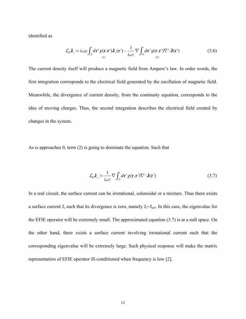
identified as

LEJs = iωµ dr 'g(r,r ')Js (r ')

S∫ −(1)

1iωε∇ dr 'g(r,r ')∇ '⋅J(r ')

S∫(2)

(3.6)

The current density itself will produce a magnetic field from Ampere’s law. In order words, the

first integration corresponds to the electrical field generated by the oscillation of magnetic field.

Meanwhile, the divergence of current density, from the continuity equation, corresponds to the

idea of moving charges. Thus, the second integration describes the electrical field created by

changes in the system.

As ω approaches 0, term (2) is going to dominate the equation. Such that

LEJs !

1iωε∇ dr 'g(r,r ')∇ '⋅J(r ')

S∫ (3.7)

In a real circuit, the surface current can be irrotational, solenoidal or a mixture. Thus there exists

a surface current Js such that its divergence is zero, namely Js=Jsol. In this case, the eigenvalue for

the EFIE operator will be extremely small. The approximated equation (3.7) is at a null space. On

the other hand, there exists a surface current involving irrotational current such that the

corresponding eigenvalue will be extremely large. Such physical response will make the matrix

representation of EFIE operator ill-conditioned when frequency is low [2].

  13  

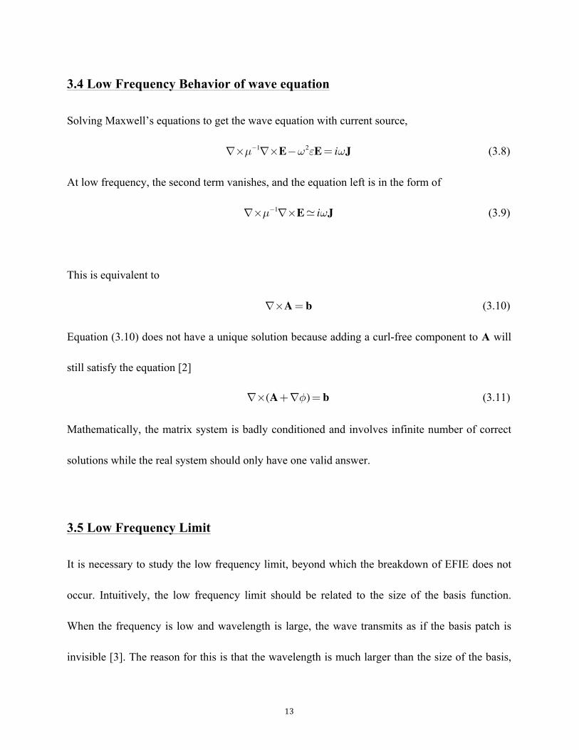
3.4 Low Frequency Behavior of wave equation

Solving Maxwell’s equations to get the wave equation with current source,

∇×µ−1∇×E−ω2εE= iωJ (3.8)

At low frequency, the second term vanishes, and the equation left is in the form of

∇×µ−1∇×E! iωJ (3.9)

This is equivalent to

∇×A= b (3.10)

Equation (3.10) does not have a unique solution because adding a curl-free component to A will

still satisfy the equation [2]

∇×(A+∇φ)= b (3.11)

Mathematically, the matrix system is badly conditioned and involves infinite number of correct

solutions while the real system should only have one valid answer.

3.5 Low Frequency Limit

It is necessary to study the low frequency limit, beyond which the breakdown of EFIE does not

occur. Intuitively, the low frequency limit should be related to the size of the basis function.

When the frequency is low and wavelength is large, the wave transmits as if the basis patch is

invisible [3]. The reason for this is that the wavelength is much larger than the size of the basis,

  14  

so that the information of the basis function is hardly seen by the wave. Due to the finite

computational precision, only large values can be collected and the smooth part of the EFIE

matrix is hard to obtain.

  15  

4. Formulation of Augmented Electric Field Integral

Equation (AEFIE)

4.1 Motivation

Full-wave electromagnetic modeling of microelectronic structure is an important method to

predict the functionality of a design. It is better than the quasi-static method as the latter is not

accurate at high frequencies. EFIE is one of the full-wave modeling techniques that covers a

wide frequency band. However, a problem arises due to the low frequency breakdown described

in the previous section. The main reason for the occurrence of low frequency breakdown is the

limitation of computer memory, which cannot distinguish vector and scalar potentials at low

frequency. In order to eliminate the low frequency problem, many techniques are implemented to

separate the calculation involving vector and scalar potentials. The loop-tree method is one of

them. However, the implementation of this method consumes a lot of memory to search for

specific loops and trees, which is not practical for large-scale structures [3]. The augmented

electric field integral equation includes charges as an extra parameter, which separates the

contributions of the vector and scalar potential. In addition to that, an appropriate scaling method

should be applied to account for precision limitation of computations in order to prevent from

low frequency breakdown [2].

  16  

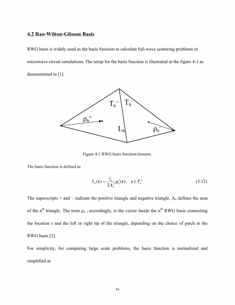
4.2 Rao-Wilton-Glisson Basis

RWG basis is widely used as the basis function to calculate full-wave scattering problems in

microwave circuit simulations. The setup for the basis function is illustrated in the figure 4-1 as

demonstrated in [1].

Figure 4-1 RWG basis function/element.

The basis function is defined as

Λn (r)=

ln2A±

n

ρ±n (r), r∈Tn

± (3.12)

The superscripts + and – indicate the positive triangle and negative triangle. An defines the area

of the nth triangle. The term ρn , accordingly, is the vector inside the nth RWG basis connecting

the location r and the left or right tip of the triangle, depending on the choice of patch in the

RWG basis [3].

For simplicity, for computing large scale problems, the basis function is normalized and

simplified as

  17  

Λn (r)=

r−r+

2An+ , r∈T +

n

r−r−

2An− , r∈T −n

0, , elsewhere

⎧

⎨

⎪⎪⎪⎪⎪⎪⎪⎪⎪

⎩

⎪⎪⎪⎪⎪⎪⎪⎪⎪

(3.13)

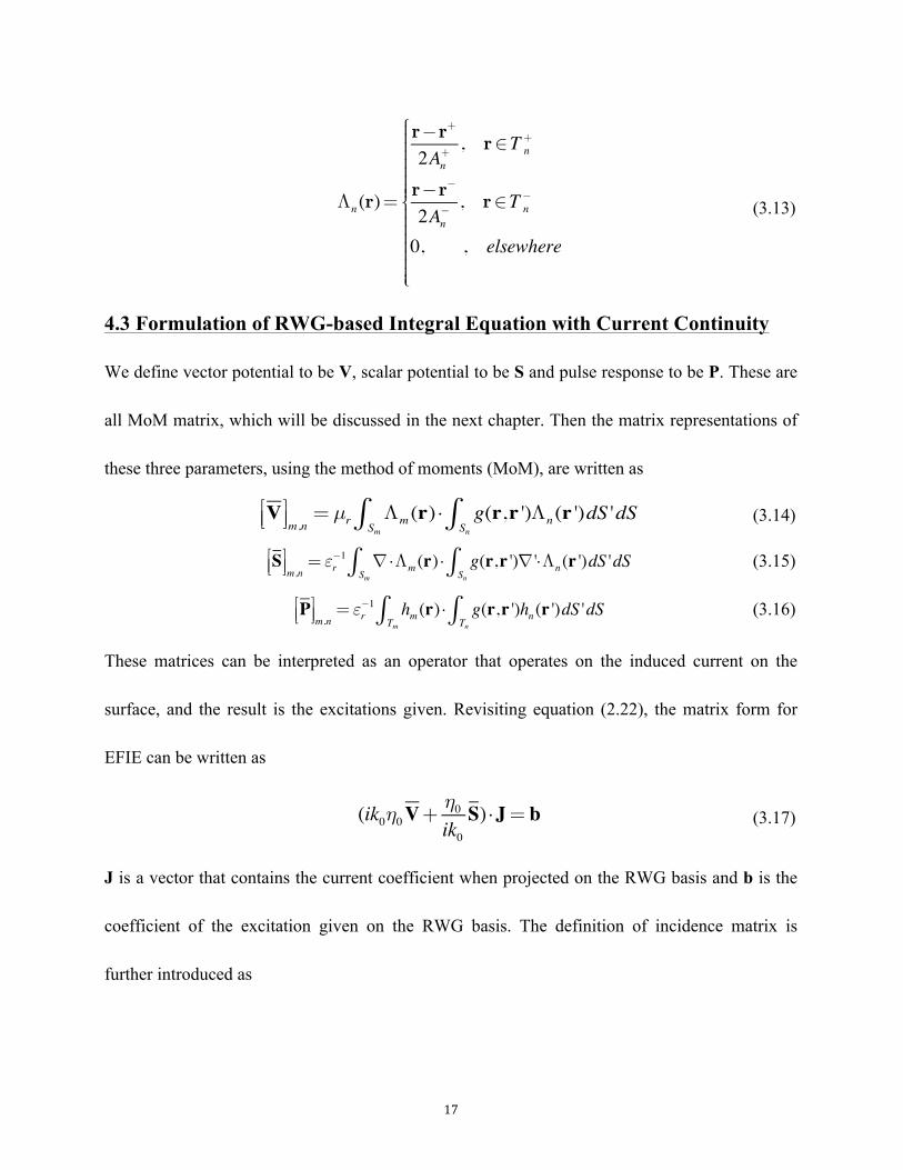
4.3 Formulation of RWG-based Integral Equation with Current Continuity

We define vector potential to be V, scalar potential to be S and pulse response to be P. These are

all MoM matrix, which will be discussed in the next chapter. Then the matrix representations of

these three parameters, using the method of moments (MoM), are written as

V⎡⎣⎢⎤⎦⎥m,n = µr Λm (r)⋅ g(r,r ')Λn (r ')dS 'dS

Sn∫Sm

∫ (3.14)

S⎡⎣⎢⎤⎦⎥m,n = εr

−1 ∇⋅Λm (r)⋅ g(r,r ')∇ '⋅Λn (r ')dS 'dSSn∫Sm

∫ (3.15)

P⎡⎣⎢⎤⎦⎥m,n = εr

−1 hm (r)⋅ g(r,r ')hn (r ')dS 'dSTn∫Tm

∫ (3.16)

These matrices can be interpreted as an operator that operates on the induced current on the

surface, and the result is the excitations given. Revisiting equation (2.22), the matrix form for

EFIE can be written as

(ik0η0V+

η0ik0S)⋅J= b (3.17)

J is a vector that contains the current coefficient when projected on the RWG basis and b is the

coefficient of the excitation given on the RWG basis. The definition of incidence matrix is

further introduced as

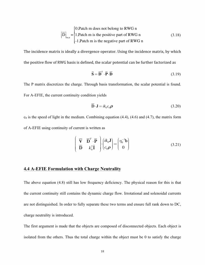
  18  

D⎡⎣⎢⎤⎦⎥m,n

=0,Patch m does not belong to RWG n1,Patch m is the positive part of RWG n-1,Patch m is the negative part of RWG n

⎧

⎨

⎪⎪⎪⎪

⎩⎪⎪⎪⎪

(3.18)

The  incidence  matrix  is  ideally  a  divergence  operator.  Using  the  incidence  matrix,  by  which  

the  positive  flow  of  RWG  basis  is  defined,  the  scalar  potential  can  be  further  factorized  as      

S=DT⋅P ⋅D (3.19)

The P matrix discretizes the charge. Through basis transformation, the scalar potential is found.

For A-EFIE, the current continuity condition yields

D⋅J = ik0c0ρ (3.20)

c0 is the speed of light in the medium. Combining equation (4.4), (4.6) and (4.7), the matrix form

of A-EFIE using continuity of current is written as

V DT⋅P

D k20 I

⎛

⎝

⎜⎜⎜⎜⎜⎜

⎞

⎠

⎟⎟⎟⎟⎟⎟⎟⋅ik0Jc0ρ⎛

⎝⎜⎜⎜⎞

⎠⎟⎟⎟⎟=η0−1b0

⎛

⎝⎜⎜⎜⎜

⎞

⎠⎟⎟⎟⎟ (3.21)

 

4.4 A-EFIE Formulation with Charge Neutrality

The above equation (4.8) still has low frequency deficiency. The physical reason for this is that

the current continuity still contains the dynamic charge flow. Irrotational and solenoidal currents

are not distinguished. In order to fully separate these two terms and ensure full rank down to DC,

charge neutrality is introduced.

The first argument is made that the objects are composed of disconnected objects. Each object is

isolated from the others. Thus the total charge within the object must be 0 to satisfy the charge

  19  

neutrality condition. ρr is introduced to represent the vector of charges in reduced form. The

forward matrix and backward matrix are defined to map the transformation between ρr and ρ.

ρr = F ⋅ρ

ρ= B⋅ρr (3.22)

Then in the equation (4.8), the total charge is replaced with changes inside each spanning tree.

The Augmented EFIE formulation is modified as

V DT⋅P⋅B

F ⋅D k20 Ir

⎛

⎝

⎜⎜⎜⎜⎜⎜

⎞

⎠

⎟⎟⎟⎟⎟⎟⎟⋅ik0Jc0ρr

⎛

⎝⎜⎜⎜

⎞

⎠⎟⎟⎟⎟=η0−1b0

⎛

⎝⎜⎜⎜⎜

⎞

⎠⎟⎟⎟⎟ (3.23)

  20  

5. Method of Moments (MoM) in A-EFIE

MoM solves integral form of Maxwell’s equations. The unknowns of MoM are the equivalent

electric current elements projected on the RWG basis.

For large-scale problems, usually it is hard to directly solve the scattering field and equivalent

current on the surface. The method of moment introduces the idea of subspace projection, which

results in another name for MoM, the subspace projection method. For example, if the

formularized equation in matrix form is given by

a11 … a1n! " !am1 # amn

⎛

⎝

⎜⎜⎜⎜⎜⎜⎜⎜

⎞

⎠

⎟⎟⎟⎟⎟⎟⎟⎟⎟=

b11 … b1n! " !bm1 # bmn

⎛

⎝

⎜⎜⎜⎜⎜⎜⎜⎜

⎞

⎠

⎟⎟⎟⎟⎟⎟⎟⎟⎟ (4.1)

then the fundamental idea of MoM is to solve the following:

a11 … a1n! " !am1 # amn

⎛

⎝

⎜⎜⎜⎜⎜⎜⎜⎜

⎞

⎠

⎟⎟⎟⎟⎟⎟⎟⎟⎟

v1..vn

⎛

⎝

⎜⎜⎜⎜⎜⎜⎜⎜⎜⎜⎜

⎞

⎠

⎟⎟⎟⎟⎟⎟⎟⎟⎟⎟⎟⎟

=b11 … b1n! " !bm1 # bmn

⎛

⎝

⎜⎜⎜⎜⎜⎜⎜⎜

⎞

⎠

⎟⎟⎟⎟⎟⎟⎟⎟⎟

v1..vn

⎛

⎝

⎜⎜⎜⎜⎜⎜⎜⎜⎜⎜⎜

⎞

⎠

⎟⎟⎟⎟⎟⎟⎟⎟⎟⎟⎟⎟

(4.2)

Equation (5.2) does not directly imply equation (5.1), while using equation (5.2) will help filling

in the matrix elements of the unknowns.

In the previous section, we mentioned the usage of MoM in these three equations:

V⎡⎣⎢⎤⎦⎥m,n = µr Λm (r)⋅ g(r,r ')Λn (r ')dS 'dS

Sn∫Sm

∫ (4.3)

S⎡⎣⎢⎤⎦⎥m,n = εr

−1 ∇⋅Λm (r)⋅ g(r,r ')∇ '⋅Λn (r ')dS 'dSSn∫Sm

∫ (4.4)

P⎡⎣⎢⎤⎦⎥m,n = εr

−1 hm (r)⋅ g(r,r ')hn (r ')dS 'dSTn∫Tm

∫ (4.5)

  21  

Equations (5.3)~(5.4) utilize the method of moments to calculate vector potential and Scalar

potential by projecting the EFIE operator onto the RWG basis [1]. Equation (5.5) uses the

projection of the capacitive term in the EFIE operator onto the pulse function basis in order to

separate the irrotational and solenoidal terms.

  22  

6. Design of Graphical User Interface

6.1 Specification of Graphical User Interface

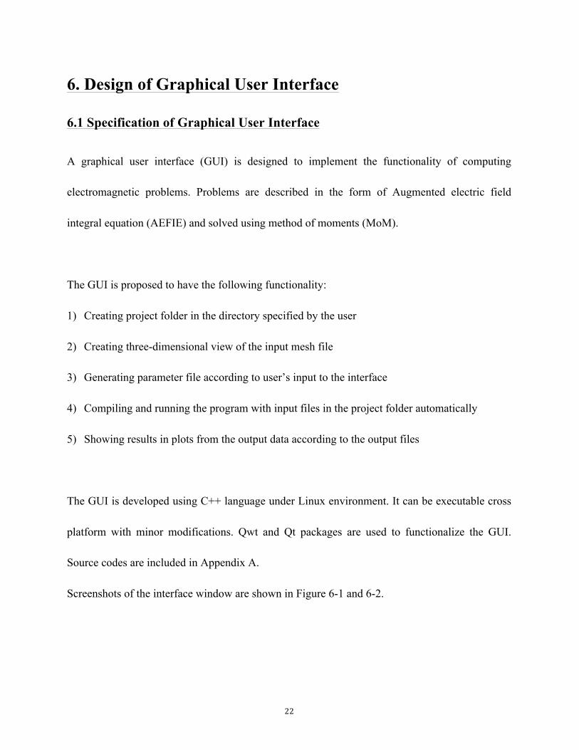
A graphical user interface (GUI) is designed to implement the functionality of computing

electromagnetic problems. Problems are described in the form of Augmented electric field

integral equation (AEFIE) and solved using method of moments (MoM).

The GUI is proposed to have the following functionality:

1) Creating project folder in the directory specified by the user

2) Creating three-dimensional view of the input mesh file

3) Generating parameter file according to user’s input to the interface

4) Compiling and running the program with input files in the project folder automatically

5) Showing results in plots from the output data according to the output files

The GUI is developed using C++ language under Linux environment. It can be executable cross

platform with minor modifications. Qwt and Qt packages are used to functionalize the GUI.

Source codes are included in Appendix A.

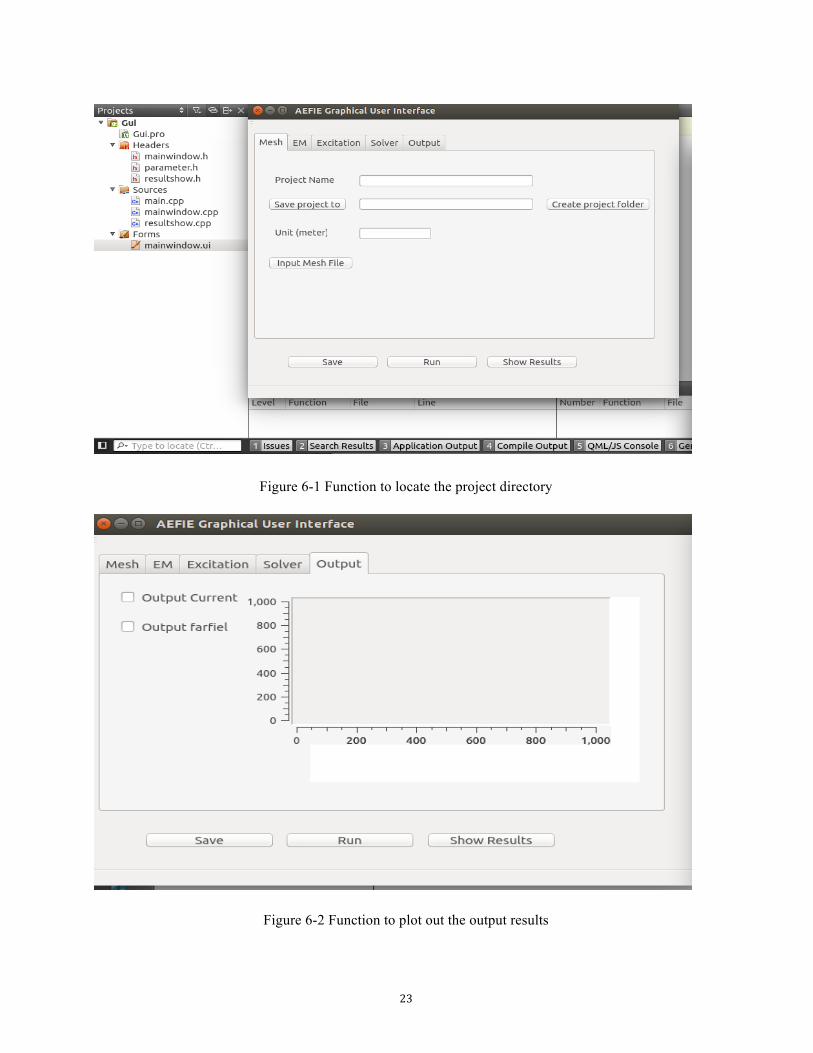
Screenshots of the interface window are shown in Figure 6-1 and 6-2.

  23  

Figure 6-1 Function to locate the project directory

Figure 6-2 Function to plot out the output results

  24  

Creating the parameter file is accomplished and the Qwt package used to show outcome results.

Linking the GUI and existing code is the next step. Creating three-dimensional view of the mesh

file will be the final task.

6.2 Instructions for using the GUI

1. Choose the location of program folder and naming it according to the input project name

2. Select the mesh file for process and click “Input mesh file” button

3. Fill in all the required blanks

4. Click on the “Save” button

5. Click on the “Run” button upon success

6. Click on the “Show Results” button, and a new window will appear with output plots

  25  

7. Conclusion

Surface integral equations are useful to model full wave electromagnetic problems. Augmented

SIEs can generally solve low frequency breakdown problems associated with EFIE operator.

However, it is suggested from simulation results that at low frequency, there are still low

frequency inaccuracies because of not being able to capture inductive behaviors of the circuit

elements.

In future work, in order to increase the accuracy of modeling a certain geometry, smaller mesh

size is required. Meanwhile, it might not be practical for the computer to handle the data with the

same algorithm. A potential area of interest is a fast algorithm to accelerate the computation and

maintain reasonable accuracy.

  26  

References

[1] W. C. Chew, M. S. Tong, B. Hu, Integral Equation Methods for Electromagnetic and Elastic

Waves, Arizona, Morgan & Claypool Publishers, 2009. [2] Zhi Guo Qian and W. C. Chew, “A quantitative study on the low frequency breakdown of

EFIE,” Comm. Comp. Phys., vol. 50, no. 5, pp. 1159-1162, 2008. [3] Weng Cho Chew, Zhi Guo Qian, Li J. Jiang and Y. P. Chen, “An augmented electric field

integral equation for layered medium Green's function,” IEEE Transactions on Antennas and Propagation., vol. 59, no. 3, pp. 960-968, 2011.

  27  

Appendix A: Source Code of GUI 1. Mainwindow.h #Ifndef MAINWINDOW_H #define MAINWINDOW_H #include <QMainWindow> #include<QFileDialog> #include<QTextStream> #include<QMessageBox> #include<QDir> #include<QString> #include<QDebug> #include<QTextStream> #include<QApplication> #include<QFileDialog> #include<QTextStream> #include<QMessageBox> #include<QDir> #include<QString> #include<QFile> #include<QDebug> #include<QTextStream> #include <QApplication> #include <qmath.h> #include <QVector> #include <qwt_plot.h> #include <qwt_plot_curve.h> #include <qwt_plot_magnifier.h> #include <qwt_plot_panner.h> #include <qwt_legend.h> #include "parameter.h" namespace Ui { class MainWindow; } class MainWindow : public QMainWindow

  28  

{ Q_OBJECT public: explicit MainWindow(QWidget *parent = 0); ~MainWindow(); void writefile(); private slots: void on_SaveButton_clicked(); void on_RunButton_clicked(); void on_ExitButton_clicked(); void on_pushButton_clicked(); void on_pushButton_2_clicked(); void on_lineEdit_3_textChanged(); void on_lineEdit_textEdited(const QString &arg1); void on_pushButton_3_clicked(); void on_lineEdit_11_textEdited(const QString &arg1); void on_lineEdit_19_textEdited(const QString &arg1); void on_lineEdit_20_textEdited(const QString &arg1); void on_checkBox_clicked(); void on_checkBox_2_clicked(); void on_checkBox_3_clicked();

  29  

void on_checkBox_4_clicked(); void on_checkBox_5_clicked(); void on_checkBox_8_clicked(); void on_checkBox_6_clicked(); void on_checkBox_7_clicked(); void on_checkBox_9_clicked(); void on_checkBox_11_clicked(); void on_checkBox_13_clicked(); void on_checkBox_10_clicked(); void on_checkBox_12_clicked(); void on_checkBox_14_clicked(); void on_checkBox_15_clicked(); void on_checkBox_16_clicked(); void on_checkBox_17_clicked(); void on_checkBox_18_clicked(); private: Ui::MainWindow *ui; parameter myparameter; }; #endif // MAINWINDOW_H

  30  

2. Mainwindow.cpp #include "mainwindow.h" #include "ui_mainwindow.h" #include "mainwindow_2.h" MainWindow::MainWindow(QWidget *parent) : QMainWindow(parent), ui(new Ui::MainWindow) { ui->setupUi(this); } MainWindow::~MainWindow() { delete ui; } void MainWindow::writefile() { QFile mFile(myparameter.mesh_project_name+".para"); if(!mFile.open(QFile::WriteOnly | QFile::Text)) { qDebug() <<"Could not open file for writing"; return; } QTextStream out(&mFile); //out<<"Hello world"; out<<"PROJECTNAME: "; out<<myparameter.mesh_project_name<<'\n'; out<<"MESHUNIT: "; out<<myparameter.mesh_unit<<'\n'; out<<"#FREQUENCYSWEEP: "; out<<myparameter.frequency_lower_bound<<" "<<myparameter.frequency_higher_bound<<" "<<myparameter.number_of_frequency<<'\n'; out<<"BACKGROUND: \n"; out<<QString::number(myparameter.background_medium_eps_r.toFloat(),'f',6) <<" "<<QString::number(myparameter.background_medium_eps_i.toFloat(),'f',6)

  31  

<<" "<<QString::number(myparameter.background_medium_mu_r.toFloat(),'f',6)<<" "<<QString::number(myparameter.background_medium_mu_i.toFloat(),'f',6) <<" "<<QString::number(myparameter.background_medium_sigma.toFloat(),'e',6)<<'\n'; out<<"EMPARAS: 1\n"; out<<" "<<QString::number(myparameter.medium_eps_r.toFloat(),'f',6) <<" "<<QString::number(myparameter.medium_eps_i.toFloat(),'f',6) <<" "<<QString::number(myparameter.medium_mu_r.toFloat(),'f',6) <<" "<<QString::number(myparameter.medium_mu_i.toFloat(),'f',6) <<" "<<QString::number(myparameter.medium_sigma.toFloat(),'f',1) <<" "<<QString::number(myparameter.medium_thickness.toFloat(),'g',2)<<'\n'; out<<"SOLVER: "; out<<myparameter.solver<<'\n'; out<<"SOLVERMETHOD: "; out<<myparameter.solver_method<<'\n'; out<<"ACCURACYLEVEL: "; out<<myparameter.accuracy_level; out<<"EXCITATIONTYPE: "; out<<myparameter.excitation_type; out<<"PLANEWAVE: "; out<<ui->lineEdit_16->text()<<" "<<ui->lineEdit_18->text()<<" "<<ui->lineEdit_21->text()<<'\n'; out<<"PLANEWAVEOBS: "; out<<ui->lineEdit_25->text()<<" "<<ui->lineEdit_24->text()<<'\n'; out<<" "<<ui->lineEdit_23->text()<<" "<<ui->lineEdit_22->text()<<'\n'; out<<" "<<ui->lineEdit_12->text()<<" "<<ui->lineEdit_17->text()<<'\n'; out<<"POINTSOURCE: "; out<<" "<<ui->lineEdit_26->text()<<" "<<ui->lineEdit_29->text()<<" "<<ui->lineEdit_30->text()<<'\n'; out<<" "<<ui->lineEdit_27->text()<<" "<<ui->lineEdit_32->text()<<" "<<ui->lineEdit_31->text()<<'\n'; out<<"NEARFIELDOBS: 3"; out<<" "<<ui->lineEdit_40->text()<<" "<<ui->lineEdit_34->text()<<" "<<ui->lineEdit_28->text()<<'\n';

  32  

out<<" "<<ui->lineEdit_39->text()<<" "<<ui->lineEdit_38->text()<<'\n'; out<<" "<<ui->lineEdit_36->text()<<" "<<ui->lineEdit_35->text()<<'\n'; out<<" "<<ui->lineEdit_37->text()<<" "<<ui->lineEdit_33->text()<<'\n'; out<<"GMRESPARAS: "; out<<" "<<ui->lineEdit_42->text()<<" "<<ui->lineEdit_45->text()<<" "<<ui->lineEdit_41->text()<<'\n'; out<<"FMAPARAS: -1 "; out<<ui->lineEdit_44->text()<<" "<<ui->lineEdit_46->text()<<" "<<ui->lineEdit_43->text()<<'\n'; out<<"NUMBEROBJECTS: "; out<<ui->lineEdit_47->text()<<'\n'; out<<"FMAOBJECTS: "<<ui->lineEdit_49->text()<<'\n'<<" 0"; mFile.flush(); mFile.close(); } void MainWindow::on_SaveButton_clicked() { myparameter.mesh_unit=ui->lineEdit->text().toDouble(); //Medium Page myparameter.background_medium_eps_r=ui->lineEdit_4->text(); myparameter.background_medium_eps_i=ui->lineEdit_6->text(); myparameter.background_medium_mu_r=ui->lineEdit_8->text(); myparameter.background_medium_mu_i=ui->lineEdit_9->text(); myparameter.background_medium_sigma=ui->lineEdit_15->text(); myparameter.medium_eps_r=ui->lineEdit_5->text(); myparameter.medium_eps_i=ui->lineEdit_7->text(); myparameter.medium_mu_r=ui->lineEdit_10->text(); myparameter.medium_mu_i=ui->lineEdit_13->text(); myparameter.medium_sigma=ui->lineEdit_14->text();

  33  

//Excitation page myparameter.frequency_lower_bound=ui->lineEdit_11->text(); myparameter.frequency_higher_bound=ui->lineEdit_19->text(); myparameter.number_of_frequency=ui->lineEdit_20->text(); //Solver page myparameter.accuracy_level=ui->spinBox->value(); //Solver II page ui->lineEdit->setText("load"); //save to parameter file if (1==QDir::setCurrent(myparameter.home_directory+'/'+myparameter.mesh_project_name)) { writefile(); } } void MainWindow::on_RunButton_clicked() { ui->lineEdit_2->setText("run"); } void MainWindow::on_ExitButton_clicked() { MainWindow_2 * result_current = new MainWindow_2; result_current->show(); } void MainWindow::on_pushButton_clicked() { QString filename=QFileDialog::getOpenFileName( this, tr("Open File"), "/Users/QQ" "All files (*.*);;Text File (*.txt);;Music file (*.mp3);;"

  34  

); } void MainWindow::on_pushButton_2_clicked() { if (1==QDir::setCurrent(myparameter.home_directory)){ QDir().mkdir(ui->lineEdit_3->text()); //ui->lineEdit_2->setText("/Users/QQ"); QMessageBox::information(0,"FYI","successfully created"); } } void MainWindow::on_lineEdit_3_textChanged() { myparameter.mesh_project_name=ui->lineEdit_3->text(); } void MainWindow::on_pushButton_3_clicked() { QString dir = QFileDialog::getExistingDirectory(this,tr("open directory"),"/Users/QQ", QFileDialog::ShowDirsOnly |QFileDialog::DontResolveSymlinks); ui->lineEdit_2->setText(dir); myparameter.home_directory=dir; } void MainWindow::on_checkBox_clicked() { if(ui->checkBox->isChecked()) myparameter.solver_method=1; }

  35  

void MainWindow::on_checkBox_2_clicked() { if(ui->checkBox_2->isChecked()) myparameter.solver_method=2; } void MainWindow::on_checkBox_9_clicked() { if(ui->checkBox_9->isChecked()) myparameter.solver_method=3; } void MainWindow::on_checkBox_3_clicked() { if(ui->checkBox_3->isChecked()) myparameter.solver_method=4; } void MainWindow::on_checkBox_4_clicked() { if(ui->checkBox_4->isChecked()) myparameter.solver=1; } void MainWindow::on_checkBox_5_clicked() { if(ui->checkBox_5->isChecked()) myparameter.solver=2; } void MainWindow::on_checkBox_11_clicked() { if(ui->checkBox_11->isChecked()) myparameter.solver=3; } void MainWindow::on_checkBox_13_clicked() { if(ui->checkBox_13->isChecked())

  36  

myparameter.solver=4; } void MainWindow::on_checkBox_7_clicked() { if(ui->checkBox_7->isChecked()) myparameter.solver=5; } void MainWindow::on_checkBox_10_clicked() { if(ui->checkBox_10->isChecked()) myparameter.solver=6; } void MainWindow::on_checkBox_12_clicked() { if(ui->checkBox_12->isChecked()) myparameter.solver=7; } void MainWindow::on_checkBox_14_clicked() { if(ui->checkBox_14->isChecked()) myparameter.excitation_type=1; } void MainWindow::on_checkBox_15_clicked() { if(ui->checkBox_15->isChecked()) myparameter.excitation_type=2; } void MainWindow::on_checkBox_16_clicked() { if(ui->checkBox_16->isChecked()) myparameter.observation_coordinate=1; }

  37  

void MainWindow::on_checkBox_17_clicked() { if(ui->checkBox_17->isChecked()) myparameter.observation_coordinate=2; } void MainWindow::on_checkBox_18_clicked() { if(ui->checkBox_18->isChecked()) myparameter.observation_coordinate=3; }