Embed Size (px)
Citation preview
Method for environmental noise estimation via
injection tests for ground-based gravitational wave
detectors
T. Washimi∗,1, T. Yokozawa2, T. Tanaka2, Y. Itoh3, J. Kume4,5,
J. Yokoyama4,5
1Gravitational Wave Science Project (GWSP), Kamioka branch, National
Astronomical Observatory of Japan (NAOJ), Kamioka-cho, Hida City, Gifu 506-1205,
Japan2Institute for Cosmic Ray Research (ICRR), KAGRA Observatory, The University of
Tokyo, Kamioka-cho, Hida City, Gifu 506-1205, Japan3Osaka city university, Sugimoto Sumiyoshi-ku, Osaka City, Osaka 558-8585, Japan4Research Center for the Early Universe (RESCEU), Graduate School of Science,
The University of Tokyo, Hongo, Bunkyo-ku, Tokyo 113-0033, Japan5Department of Physics, Graduate School of Science, The University of Tokyo,
Hongo, Bunkyo-ku, Tokyo 113-0033, Japan
E-mail: [email protected]
Abstract. Environmental noise is one of the critical issues for the observation of
gravitational waves, but is difficult to predict in advance. Therefore, to evaluate the
adverse impact of environmental noise on the detector sensitivity, understanding the
detector response to the environmental noise in actual setup is crucial, for both the
observation and future upgrades. In this paper, we introduce and verify a new method
of the environmental noise injection test based on the post-observation commissioning
of KAGRA. This new method (response function model) includes the frequency
conversion and nonlinearity of power, which are the effects that are not considered
in the current model (coupling function model) used in LIGO and Virgo. We also
confirmed the validity of our method by applying it to an environmental noise-enriched
dataset and successfully reproducing them.
1. Introduction
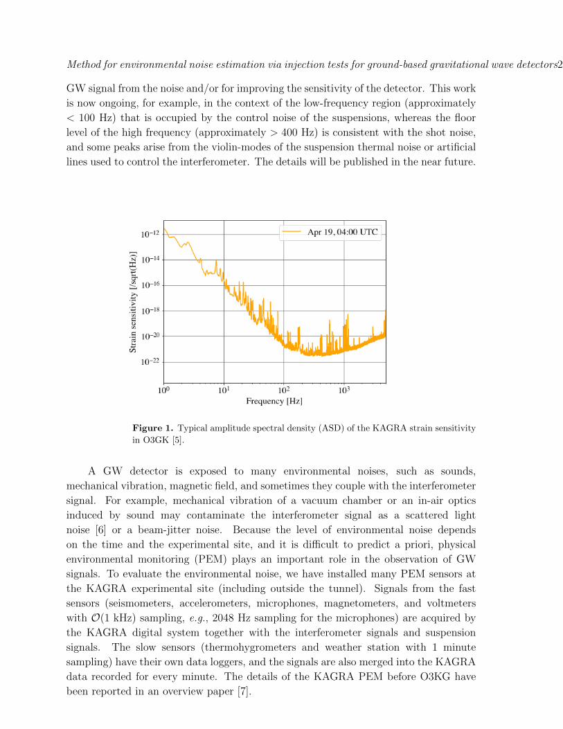
Since the first detection of gravitational waves (GW) was achieved by the advanced
LIGO [1], more than 50 GW events [2, 3] have been detected by 3-detectors; LLO, LHO
in US, and Virgo in Italy. The 4th GW detector, KAGRA, constructed in Japan, is a
unique detector that is in an underground facility and that cools the test-mass mirrors to
reduce seismic noise and thermal noise [4]. KAGRA performed the first joint observation
run (O3GK) with GEO600 in Germany, from April 7 to 21, 2020 [5]. The typical strain
sensitivity of the KAGRA interferometer in O3GK is shown in Figure 1. Understanding
the noise components, the so called ”Noise budget”, is important for distinguishing a
arX
iv:2
012.
0929
4v3
[gr
-qc]
7 M
ay 2
021
Method for environmental noise estimation via injection tests for ground-based gravitational wave detectors2
GW signal from the noise and/or for improving the sensitivity of the detector. This work
is now ongoing, for example, in the context of the low-frequency region (approximately
< 100 Hz) that is occupied by the control noise of the suspensions, whereas the floor
level of the high frequency (approximately > 400 Hz) is consistent with the shot noise,
and some peaks arise from the violin-modes of the suspension thermal noise or artificial
lines used to control the interferometer. The details will be published in the near future.
Figure 1. Typical amplitude spectral density (ASD) of the KAGRA strain sensitivity
in O3GK [5].
A GW detector is exposed to many environmental noises, such as sounds,
mechanical vibration, magnetic field, and sometimes they couple with the interferometer
signal. For example, mechanical vibration of a vacuum chamber or an in-air optics
induced by sound may contaminate the interferometer signal as a scattered light
noise [6] or a beam-jitter noise. Because the level of environmental noise depends
on the time and the experimental site, and it is difficult to predict a priori, physical
environmental monitoring (PEM) plays an important role in the observation of GW
signals. To evaluate the environmental noise, we have installed many PEM sensors at
the KAGRA experimental site (including outside the tunnel). Signals from the fast
sensors (seismometers, accelerometers, microphones, magnetometers, and voltmeters
with O(1 kHz) sampling, e.g., 2048 Hz sampling for the microphones) are acquired by
the KAGRA digital system together with the interferometer signals and suspension
signals. The slow sensors (thermohygrometers and weather station with 1 minute
sampling) have their own data loggers, and the signals are also merged into the KAGRA
data recorded for every minute. The details of the KAGRA PEM before O3KG have
been reported in an overview paper [7].
Method for environmental noise estimation via injection tests for ground-based gravitational wave detectors3
The power spectrum density (PSD) of the interferometer signal S(f) can be divided
into a component SPEM(f) caused by environmental noise P (f) monitored by a PEM
sensor, and other noise Sother(f) that is independent of P (f):
S(f) = SPEM(f) + Sother(f). (1)
One purpose of the PEM is to estimate the environmental noise SPEM(f) for an
observation mode.
2. Concept of the PEM injection
PEM injection is a technique to estimate the environmental noise SPEM(f) in the
interferometer signal S(f) by increasing the environmental noise artificially. In this
paper, Sbkg(f) and Pbkg(f) denote PSDs for the strain signal and the PEM signal for
the background data, respectively, and Sinj(f) and Pinj(f) denote those for the injection
data.
Because sometimes Sinj(f) is not larger than Sbkg(f) adequately, the transfer
function is not available for PEM injection analysis. If Pinj(f) is sufficiently larger
than Pbkg(f), SPEM(f) can be derived, even though it is below the sensitivity Sbkg(f).
2.1. The coupling function model
A coupling function model has been developed in LIGO [8, 9] and widely used in LIGO,
Virgo [10], and KAGRA. In this model, PEM projection SPEM(f) for the background
data is estimated as
SPEM(f) = C2(f) · Pbkg(f) =Sinj(f)− Sbkg(f)
Pinj(f)− Pbkg(f)· Pbkg(f), (2)
where C(f) is the coupling function ‡. The excess in the interferometer ∆S =
Sinj(f) − Sbkg(f) is not always significant. In case of ∆S(f) < Sbkg(f), the upper
limit of the coupling function and the PEM projection are expressed as
C2UL(f) =
Sbkg(f)
Pinj(f)− Pbkg(f), (3)
SPEM,UL(f) = C2UL(f) · Pbkg(f), (4)
instead of the coupling function and PEM projection themselves. If the injected noise
∆P = Pinj(f)−Pbkg(f) is not sufficient, neither the PEM projection nor its upper limit
are evaluated for such frequency.
This coupling function model is based on the following hypothesis: (1) Frequency
conservation (no frequency conversion such as harmonics, side bands, etc.), (2) Linearity
of PSD between the interferometer and environmental noise (e.g., SPEM doubles if P (f)
doubles), and (3) Stability of the interferometer during measurement. However, they
are not always satisfied. For example, the scattered light noise is expressed as
hscat(t) = K sin
(8π
λx(t)
), (5)
‡ For the ASD,√SPEM(f) = C(f)
√Pbkg(f)
Method for environmental noise estimation via injection tests for ground-based gravitational wave detectors4
where x(t) is the low frequency (< 10 Hz) vibration (displacement) of the surface on
which the ghost beam is scattered (e.g., the inner surface of the vacuum chamber), λ is
the wavelength of light, and K is a constant [6]. The PSD of hscat(t) neither has linearity
nor frequency conservation in general. If there are some moving peaks or bumps that
are independent of the environmental noise, they can be larger than the threshold of
∆S and make overestimation in the PEM projection result, it means some finite excess
caused by instability (time dependence) of the interferometer itself and not be coming
from the PEM injection.
2.2. The response function and non-linear model
To include frequency conversion and nonlinearity, we expand the Equation (2) to the
following formula:
SPEM(f) =
∫ [R(f, f ′) · Pbkg(f
′) · ε]df ′, (6)
where R(f, f ′) is the response function §, ε = ε(f, f ′, Pbkg) is a function that describes
some nonlinearity (ε = 1 for linear response).
The coupling function model is included as
RCF(f, f ′) =Sinj(f)− Sbkg(f)
Pinj(f ′)− Pbkg(f ′)· δ(f − f ′), ε = 1. (7)
When a single frequency (f ′) environmental noise is injected, the kernel of the integral
can be measured as follows:
R(f, f ′) · ε =Sinj(f)− Sbkg(f)
Pinj(f ′)− Pbkg(f ′)· 1
∆f ′, (8)
where ∆f ′ is the frequency resolution of these PSDs. To take stability of the
interferometer into account in the analysis quantitatively, the threshold of ∆S needs
to be determined via a statistical treatment.
3. Experimental setup
The measurements were performed on June 11, 2020, in the post-commissioning term
of the O3GK. In this paper, the error signal (non-calibrated raw signal) of the KAGRA
interferometer was used instead of the strain or differential arm length (DARM) because
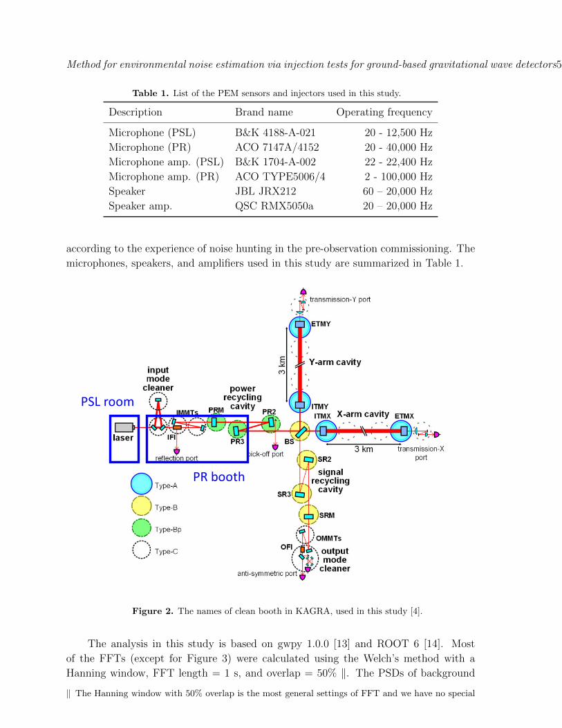
the accurate calibration was not realized for this day. Figure 2 presents a schematic view
of the KAGRA apparatus; laser path, mirrors, vacuum chambers, and clean booths. In
this study, we focused on the acoustic noise at the input optics [12] area, since it
is known that the pre-mode cleaner in the PSL (pre-stabilized laser) room and the
scattered light on the bellows between the IMC (input mode cleaner) and the IFI (input
Faraday isolator) in the PR (power recycling) booth are sensitive to the acoustic noise,
§ The response function is widely used in the field of fast-neutron detector [11].
Method for environmental noise estimation via injection tests for ground-based gravitational wave detectors5
Table 1. List of the PEM sensors and injectors used in this study.
Description Brand name Operating frequency
Microphone (PSL) B&K 4188-A-021 20 - 12,500 Hz
Microphone (PR) ACO 7147A/4152 20 - 40,000 Hz
Microphone amp. (PSL) B&K 1704-A-002 22 - 22,400 Hz
Microphone amp. (PR) ACO TYPE5006/4 2 - 100,000 Hz
Speaker JBL JRX212 60 – 20,000 Hz
Speaker amp. QSC RMX5050a 20 – 20,000 Hz
according to the experience of noise hunting in the pre-observation commissioning. The
microphones, speakers, and amplifiers used in this study are summarized in Table 1.
PSL room
PR booth
Figure 2. The names of clean booth in KAGRA, used in this study [4].
The analysis in this study is based on gwpy 1.0.0 [13] and ROOT 6 [14]. Most
of the FFTs (except for Figure 3) were calculated using the Welch’s method with a
Hanning window, FFT length = 1 s, and overlap = 50% ‖. The PSDs of background
‖ The Hanning window with 50% overlap is the most general settings of FFT and we have no special
Method for environmental noise estimation via injection tests for ground-based gravitational wave detectors6
are evaluated by approximately 5 min data.
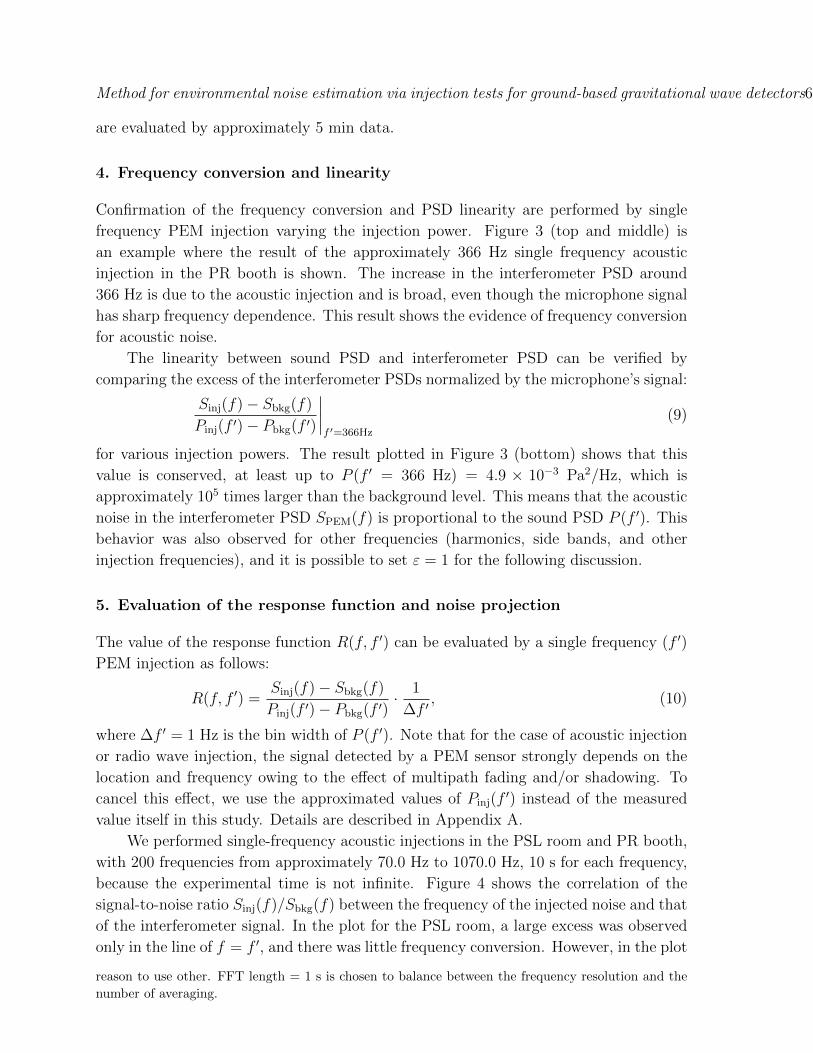
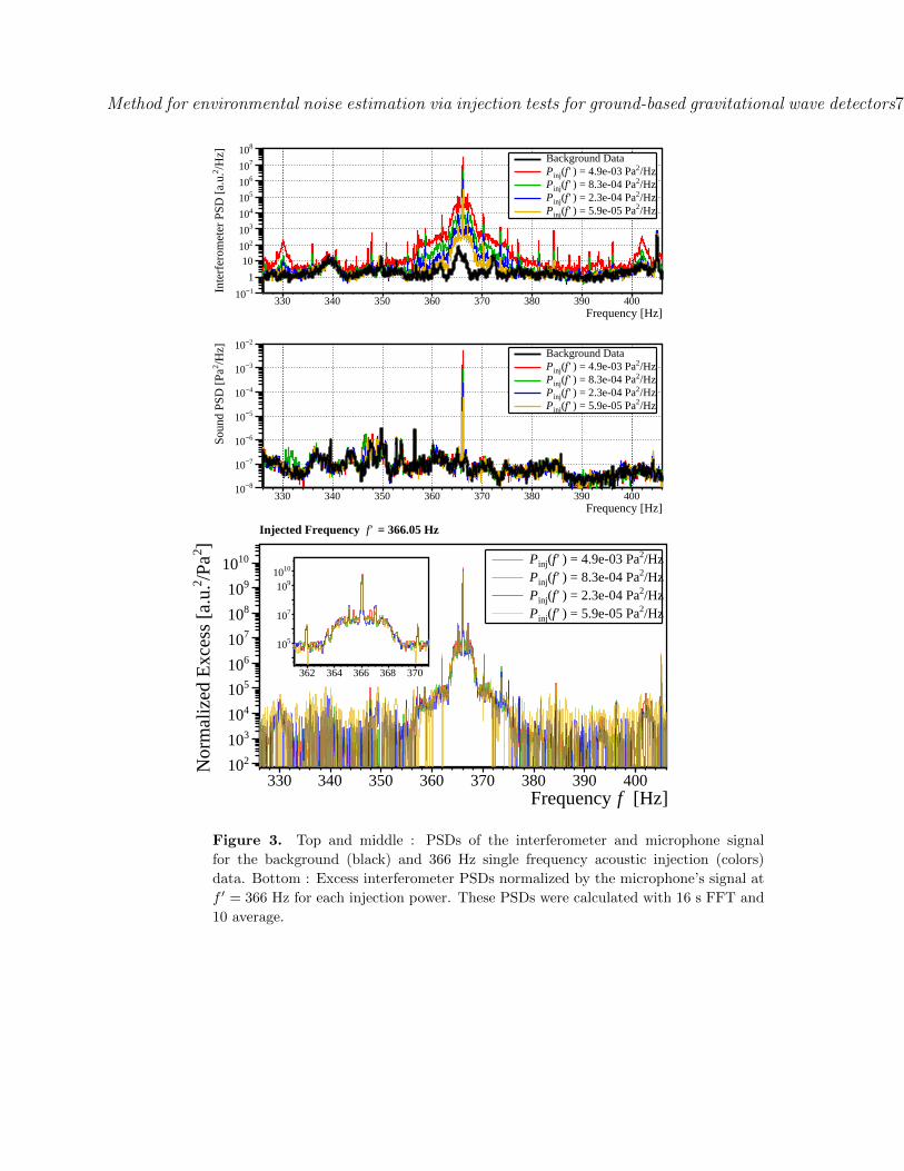
4. Frequency conversion and linearity
Confirmation of the frequency conversion and PSD linearity are performed by single
frequency PEM injection varying the injection power. Figure 3 (top and middle) is
an example where the result of the approximately 366 Hz single frequency acoustic
injection in the PR booth is shown. The increase in the interferometer PSD around
366 Hz is due to the acoustic injection and is broad, even though the microphone signal
has sharp frequency dependence. This result shows the evidence of frequency conversion
for acoustic noise.
The linearity between sound PSD and interferometer PSD can be verified by
comparing the excess of the interferometer PSDs normalized by the microphone’s signal:
Sinj(f)− Sbkg(f)
Pinj(f ′)− Pbkg(f ′)
∣∣∣∣f ′=366Hz
(9)
for various injection powers. The result plotted in Figure 3 (bottom) shows that this
value is conserved, at least up to P (f ′ = 366 Hz) = 4.9 × 10⁻³ Pa2/Hz, which is
approximately 105 times larger than the background level. This means that the acoustic
noise in the interferometer PSD SPEM(f) is proportional to the sound PSD P (f ′). This
behavior was also observed for other frequencies (harmonics, side bands, and other
injection frequencies), and it is possible to set ε = 1 for the following discussion.
5. Evaluation of the response function and noise projection
The value of the response function R(f, f ′) can be evaluated by a single frequency (f ′)
PEM injection as follows:
R(f, f ′) =Sinj(f)− Sbkg(f)
Pinj(f ′)− Pbkg(f ′)· 1
∆f ′, (10)
where ∆f ′ = 1 Hz is the bin width of P (f ′). Note that for the case of acoustic injection
or radio wave injection, the signal detected by a PEM sensor strongly depends on the
location and frequency owing to the effect of multipath fading and/or shadowing. To
cancel this effect, we use the approximated values of Pinj(f′) instead of the measured
value itself in this study. Details are described in Appendix A.
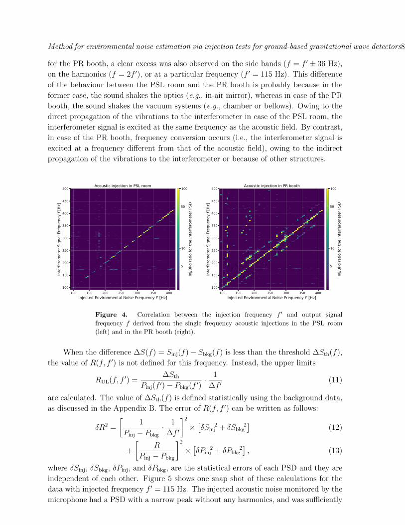
We performed single-frequency acoustic injections in the PSL room and PR booth,
with 200 frequencies from approximately 70.0 Hz to 1070.0 Hz, 10 s for each frequency,
because the experimental time is not infinite. Figure 4 shows the correlation of the
signal-to-noise ratio Sinj(f)/Sbkg(f) between the frequency of the injected noise and that
of the interferometer signal. In the plot for the PSL room, a large excess was observed
only in the line of f = f ′, and there was little frequency conversion. However, in the plot
reason to use other. FFT length = 1 s is chosen to balance between the frequency resolution and the
number of averaging.
Method for environmental noise estimation via injection tests for ground-based gravitational wave detectors7
330 340 350 360 370 380 390 400Frequency [Hz]
1−10
1
10
210
310
410
510
610
710
810
/Hz]
2In
terf
erom
eter
PSD
[a.
u.
Background Data/Hz2) = 4.9e-03 Paf'(injP/Hz2) = 8.3e-04 Paf'(injP/Hz2) = 2.3e-04 Paf'(injP/Hz2) = 5.9e-05 Paf'(injP
330 340 350 360 370 380 390 400Frequency [Hz]
8−10
7−10
6−10
5−10
4−10
3−10
2−10
/Hz]
2 S
ound
PSD
[Pa
Background Data/Hz2) = 4.9e-03 Paf'(injP/Hz2) = 8.3e-04 Paf'(injP/Hz2) = 2.3e-04 Paf'(injP/Hz2) = 5.9e-05 Paf'(injP
330 340 350 360 370 380 390 400 [Hz]fFrequency
210
310
410
510
610
710
810
910
1010
]2/P
a2
Nor
mal
ized
Exc
ess
[a.u
.
/Hz2) = 4.9e-03 Paf'(injP/Hz2) = 8.3e-04 Paf'(injP/Hz2) = 2.3e-04 Paf'(injP/Hz2) = 5.9e-05 Paf'(injP
362 364 366 368 370
510
710
910
1010
= 366.05 Hzf'Injected Frequency
Figure 3. Top and middle : PSDs of the interferometer and microphone signal
for the background (black) and 366 Hz single frequency acoustic injection (colors)
data. Bottom : Excess interferometer PSDs normalized by the microphone’s signal at
f ′ = 366 Hz for each injection power. These PSDs were calculated with 16 s FFT and
10 average.
Method for environmental noise estimation via injection tests for ground-based gravitational wave detectors8
for the PR booth, a clear excess was also observed on the side bands (f = f ′ ± 36 Hz),
on the harmonics (f = 2f ′), or at a particular frequency (f ′ = 115 Hz). This difference
of the behaviour between the PSL room and the PR booth is probably because in the
former case, the sound shakes the optics (e.g., in-air mirror), whereas in case of the PR
booth, the sound shakes the vacuum systems (e.g., chamber or bellows). Owing to the
direct propagation of the vibrations to the interferometer in case of the PSL room, the
interferometer signal is excited at the same frequency as the acoustic field. By contrast,
in case of the PR booth, frequency conversion occurs (i.e., the interferometer signal is
excited at a frequency different from that of the acoustic field), owing to the indirect
propagation of the vibrations to the interferometer or because of other structures.
100 150 200 250 300 350 400Injected Environmental Noise Frequency f ′ [Hz]
100
150
200
250
300
350
400
450
500
Inte
rfero
met
er S
igna
l Fre
quen
cy f
[Hz]
Acoustic injection in PSL room
10
100
5
50
Inj/B
kg ra
tio fo
r the
inte
rfero
met
er P
SD
100 150 200 250 300 350 400Injected Environmental Noise Frequency f ′ [Hz]
100
150
200
250
300
350
400
450
500
Inte
rfero
met
er S
igna
l Fre
quen
cy f
[Hz]
Acoustic injection in PR booth
10
100
5
50
Inj/B
kg ra
tio fo
r the
inte
rfero
met
er P
SD
Figure 4. Correlation between the injection frequency f ′ and output signal
frequency f derived from the single frequency acoustic injections in the PSL room
(left) and in the PR booth (right).
When the difference ∆S(f) = Sinj(f)− Sbkg(f) is less than the threshold ∆Sth(f),
the value of R(f, f ′) is not defined for this frequency. Instead, the upper limits
RUL(f, f ′) =∆Sth
Pinj(f ′)− Pbkg(f ′)· 1
∆f ′(11)
are calculated. The value of ∆Sth(f) is defined statistically using the background data,
as discussed in the Appendix B. The error of R(f, f ′) can be written as follows:
δR2 =
[1
Pinj − Pbkg
· 1
∆f ′
]2×[δSinj
2 + δSbkg2]
(12)
+
[R
Pinj − Pbkg
]2×[δPinj
2 + δPbkg2], (13)
where δSinj, δSbkg, δPinj, and δPbkg, are the statistical errors of each PSD and they are
independent of each other. Figure 5 shows one snap shot of these calculations for the
data with injected frequency f ′ = 115 Hz. The injected acoustic noise monitored by the
microphone had a PSD with a narrow peak without any harmonics, and was sufficiently
Method for environmental noise estimation via injection tests for ground-based gravitational wave detectors9
larger than the background level (Pinj/Pbkg ∼ 105 at f ′ = 115 Hz). Many peaks were
observed in the PSD of the interferometer signal, not only at approximately 115 Hz, but
also at the combination of the harmonics and sidebands. One remarkable point is that
the SNR at f = 230 Hz ( second harmonic) was larger than that at f = 115 Hz.
200 400 600 800 1000Frequency [Hz]
1−10
1
10
210
310
410
510
610
710
810
/Hz]
2In
terf
erom
eter
PSD
[a.
u.
Injected data
Background data
200 400 600 800 1000Frequency [Hz]
1−10
1
10
210
310
410
510
bkg
/ PS
Din
jIn
terf
erom
eter
PSD
200 400 600 800 1000Frequency [Hz]
10−10
8−10
6−10
4−10
2−10
/Hz]
2So
und
PSD
[Pa
Injection modelInjected dataBackground data
200 400 600 800 1000Frequency [Hz]
310
410
510
610
710
810
910
1010
1110)]2 /
(Hz
Pa2
R(f
,f')
[a.
u.Response Function
Upper Limit (99.7%)
Figure 5. Snap shot of the single frequency acoustic injection in the PR booth at
f ′ = 115 Hz. Top left : PSDs of the interferometer signal for injection data and
background data. Bottom left : Same as the microphone signal and the approximated
function of the injected noise. Top right : Ratio of injection PSD and background PSD
(SNR) for the interferometer signal. Bottom right : Response function and its upper
limit at f ′ = 115 Hz.
The PEM projection SPEM(f) and its upper limit are calculated as
SPEM(f) =∑f ′
[R(f, f ′) · Pbkg(f
′)]
∆f ′inj, (14)
[SPEM,UL(f)]2 =∑f ′
[RUL(f, f ′) · Pbkg(f
′) ·∆f ′inj]2, (15)
where ∆f ′inj ∼ 5 Hz is the interval of injection frequency and Pbkg(f′) is the average
of Pbkg(f′′) for f ′ − ∆f ′inj/2 ≤ f ′′ < f ′ + ∆f ′inj/2. The error of SPEM(f) is a slightly
complicated because δR(f, f ′) also contains n2bkg. However, since Pinj is much larger
than Pbkg at the injected frequency, Pbkg and δPbkg are negligible in the Equation (13) :
δR2 ' δSinj2 + δSbkg
2
(Pinj ·∆f ′)2+
[R
Pinj
· δPinj
]2. (16)
Method for environmental noise estimation via injection tests for ground-based gravitational wave detectors10
Under this approximation, the error of the PEM projection can be written as
[δSPEM(f)]2 '∑f ′
[{δR(f, f ′) · Pbkg(f
′)}2
+{R(f, f ′) · δPbkg(f
′)}2] ·∆f ′inj2. (17)
This error will be used in the discussion in the next section.
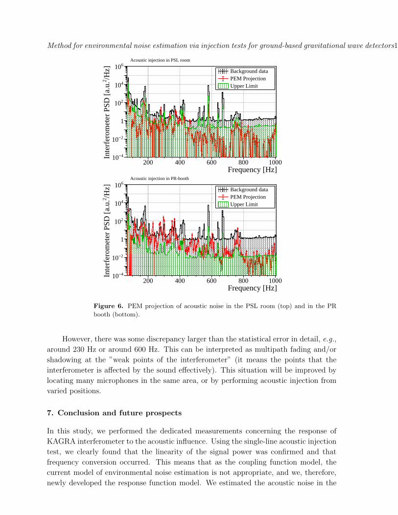
Figure 6 shows the results of PEM projections and these upper limits of acoustic
noise in the PR booth and in the PSL room. On one hand, the projected acoustic
noise in the PR booth was larger than the upper limit at most frequencies and was
dominant around 200-400 Hz. On the other hand, the projected acoustic noise in the
PSL room contributed only around 350 Hz, and was smaller than the upper limit at
most frequencies.
In case of the coupling function model, the situation is quite simple because we can
calculate the PEM projection at the frequency for ∆S(f) > ∆Sth(f) and the upper limit
for ∆S(f) < ∆Sth(f). However, in case of the coupling function model, the possibility
that there are hidden excess below ∆Sth(f) not only for the injected frequency (f ′)
but also for all frequencies (f) is considered. Finally, the upper limit is stacked up and
became about ×√
200 (the threshold ∆Sth(f) is common for all f ′) due to the integral of
f ′, where 200 is the number of injected frequencies. The results of PEM projection (red
graph in Figure 6) is meaningful only they are above the upper limit (green). Therefore,
we need for this analysis (the response function model) to inject the noise with larger
power compared to the coupling function model case.
We performed the acoustic injection with the same DAC count for both PSL room
and PR booth. For the PSL room, constructed with hard door and wall, the speaker
was located outside of the door to avoid defiling the cleanness. But for the PR booth, we
could locate the speaker inside of the clean booth. Actually, Pinj/Pbkg was about104−5
for the PR booth but Pinj/Pbkg was about 103 for the PSL room. This is a good precept
for us toward the further measurements.
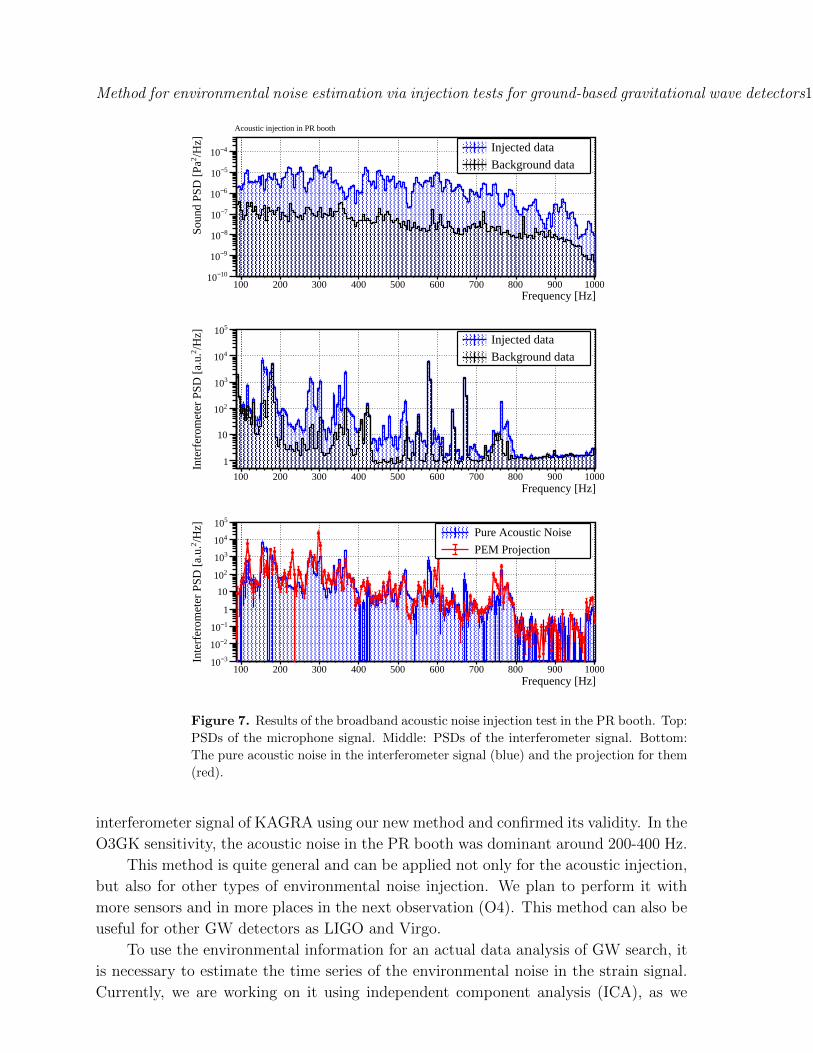
6. Test of the response function model by broadband acoustic injection
Verification of the response function model and results of PEM projection were
tested using another dataset. Here, Sbroad(f) and Pbroad(f) were the PSDs of the
interferometer and the PEM sensor, respectively, for a broadband PEM injection. The
difference Sbroad(f) − Sbkg(f) can be understood as a ”pure environmental noise” in
the interferometer signal when is is assumed that the other noises are stationary and
canceled. This difference can be predicted as
SPEM(f) =∑f ′
R(f, f ′){Pbroad(f ′)− Pbkg(f
′)}
∆f ′inj, (18)
using the response function R(f, f ′) derived from single-frequency injections. Figure 7
shows the results of the broadband acoustic noise injection test in the PR booth,
performed just after the single frequency acoustic injections. The excess in the
interferometer signal is almost consistent with the calculation from the Equation (18).
Method for environmental noise estimation via injection tests for ground-based gravitational wave detectors11
200 400 600 800 1000Frequency [Hz]
4−10
2−10
1
210
410
610
/Hz]
2In
terf
erom
eter
PSD
[a.
u.
Background dataPEM ProjectionUpper Limit
Acoustic injection in PSL room
200 400 600 800 1000Frequency [Hz]
4−10
2−10
1
210
410
610
/Hz]
2In
terf
erom
eter
PSD
[a.
u.
Background dataPEM ProjectionUpper Limit
Acoustic injection in PR-booth
Figure 6. PEM projection of acoustic noise in the PSL room (top) and in the PR
booth (bottom).
However, there was some discrepancy larger than the statistical error in detail, e.g.,
around 230 Hz or around 600 Hz. This can be interpreted as multipath fading and/or
shadowing at the ”weak points of the interferometer” (it means the points that the
interferometer is affected by the sound effectively). This situation will be improved by
locating many microphones in the same area, or by performing acoustic injection from
varied positions.
7. Conclusion and future prospects
In this study, we performed the dedicated measurements concerning the response of
KAGRA interferometer to the acoustic influence. Using the single-line acoustic injection
test, we clearly found that the linearity of the signal power was confirmed and that
frequency conversion occurred. This means that as the coupling function model, the
current model of environmental noise estimation is not appropriate, and we, therefore,
newly developed the response function model. We estimated the acoustic noise in the
Method for environmental noise estimation via injection tests for ground-based gravitational wave detectors12
100 200 300 400 500 600 700 800 900 1000Frequency [Hz]
10−10
9−10
8−10
7−10
6−10
5−10
4−10/Hz]
2So
und
PSD
[Pa
Injected data
Background data
Acoustic injection in PR booth
100 200 300 400 500 600 700 800 900 1000Frequency [Hz]
1
10
210
310
410
510
/Hz]
2In
terf
erom
eter
PSD
[a.
u.
Injected data
Background data
100 200 300 400 500 600 700 800 900 1000Frequency [Hz]
3−10
2−10
1−10
1
10
210
310
410
510
/Hz]
2In
terf
erom
eter
PSD
[a.
u.
Pure Acoustic Noise
PEM Projection
Figure 7. Results of the broadband acoustic noise injection test in the PR booth. Top:
PSDs of the microphone signal. Middle: PSDs of the interferometer signal. Bottom:
The pure acoustic noise in the interferometer signal (blue) and the projection for them
(red).
interferometer signal of KAGRA using our new method and confirmed its validity. In the
O3GK sensitivity, the acoustic noise in the PR booth was dominant around 200-400 Hz.
This method is quite general and can be applied not only for the acoustic injection,
but also for other types of environmental noise injection. We plan to perform it with
more sensors and in more places in the next observation (O4). This method can also be
useful for other GW detectors as LIGO and Virgo.
To use the environmental information for an actual data analysis of GW search, it
is necessary to estimate the time series of the environmental noise in the strain signal.
Currently, we are working on it using independent component analysis (ICA), as we
Method for environmental noise estimation via injection tests for ground-based gravitational wave detectors13
performed in iKAGRA data [15]. Although the simplest linear mixing model has been
investigated in this paper, ICA can be further extended to the case where the noise
couples nonlinearly to the strain channel. This should be useful to deal with the acoustic
noises observed in this work. We are going to improve ICA by appropriately taking into
account the environmental information, and by establishing a noise subtraction scheme
that enhances the efficiency of the GW search.
Acknowledgement
This research has made use of data, software, and web tools obtained or developed by
the KAGRA Collaboration. In this study, we were supported by KAGRA collaborators,
especially the commissioning members of the interferometer and vibration-isolation
systems, administrators of the digital system, and managers of the KAGRA experiment.
We were also helped by the LIGO project, and the Virgo project, especially Robert
Schofield & Anamaria Effler in the LIGO PEM group and Federico Paoletti & Irene Fiori
in the Virgo environmental group. We would like to thank Editage (www.editage.com)
for English language editing.
The KAGRA project is funded by the Ministry of Education, Culture, Sports,
Science and Technology (MEXT) and the Japan Society for the Promotion of Science
(JSPS). Especially this work was founded by JSPS Grant-in-Aid for Scientific Research
(S) 17H06133 and 20H05639, JSPS Grant-in-Aid for JSPS Fellows 19J01299 JSPS
Grant-in-Aid for Scientific Research on Innovative Areas 6105 20H05256, and the Joint
Research Program of the Institute for Cosmic Ray Research (ICRR) University of Tokyo
2019-F14, 2020-G12, and 2020-G21.
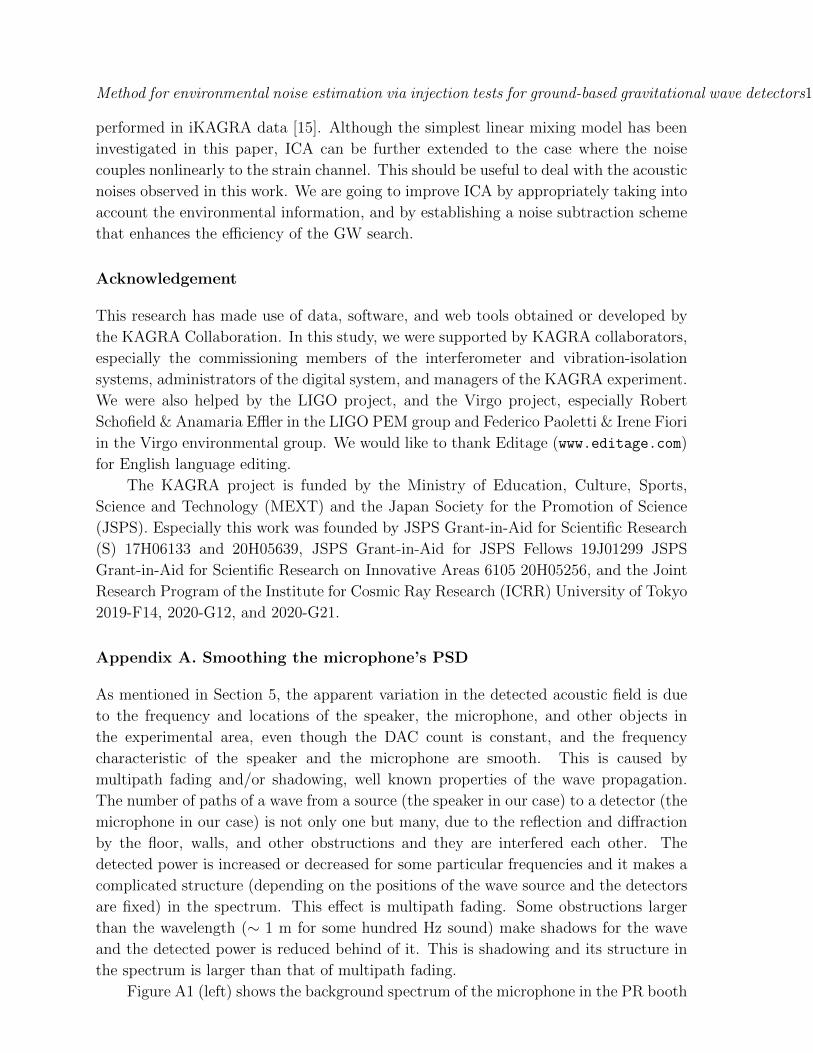
Appendix A. Smoothing the microphone’s PSD
As mentioned in Section 5, the apparent variation in the detected acoustic field is due
to the frequency and locations of the speaker, the microphone, and other objects in
the experimental area, even though the DAC count is constant, and the frequency
characteristic of the speaker and the microphone are smooth. This is caused by
multipath fading and/or shadowing, well known properties of the wave propagation.
The number of paths of a wave from a source (the speaker in our case) to a detector (the
microphone in our case) is not only one but many, due to the reflection and diffraction
by the floor, walls, and other obstructions and they are interfered each other. The
detected power is increased or decreased for some particular frequencies and it makes a
complicated structure (depending on the positions of the wave source and the detectors
are fixed) in the spectrum. This effect is multipath fading. Some obstructions larger
than the wavelength (∼ 1 m for some hundred Hz sound) make shadows for the wave
and the detected power is reduced behind of it. This is shadowing and its structure in
the spectrum is larger than that of multipath fading.
Figure A1 (left) shows the background spectrum of the microphone in the PR booth
Method for environmental noise estimation via injection tests for ground-based gravitational wave detectors14
(black), and the peak values of each line for the single-frequency injection test (blue).
Because the points that the acoustic noise affects the interferometer are different from
those of the microphone, this bias needs to be canceled. Here, the data log10 Pinj(f′) is
fitted to a polynomial function using the least-squares method. The red line in Figure A1
(left) is the result, and the histogram in the Figure A1 (right) is the difference between
the data and the function. The same procedure is also performed for the measurement
in the PSL room.
200 400 600 800 1000Frequency [Hz]
10−10
8−10
6−10
4−10
2−10
1
/ H
z]2
Soun
d PS
D [
Pa
Injected peaks
Polynomial approx.
Background data
3− 2− 1− 0 1 2 3 (Data/Function)
10log
0
2
4
6
8
10
num
ber
of p
oint
s
Figure A1. Left : PSD of the PR booth microphone for the background data (black),
the peak values for the single frequency acoustic injections (blue), and the polynomial
approximation (red). Right : Difference between the data and the function.
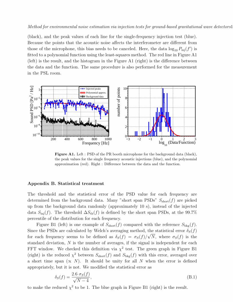
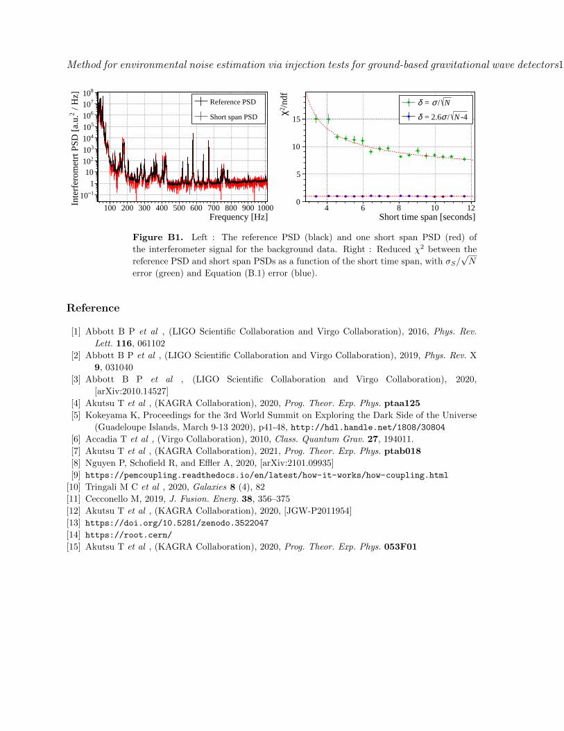
Appendix B. Statistical treatment
The threshold and the statistical error of the PSD value for each frequency are
determined from the background data. Many ”short span PSDs” Sshort(f) are picked
up from the background data randomly (approximately 10 s), instead of the injected
data Sinj(f). The threshold ∆Sth(f) is defined by the short span PSDs, at the 99.7%
percentile of the distribution for each frequency.
Figure B1 (left) is one example of Sshort(f) compared with the reference Sbkg(f).
Since the PSDs are calculated by Welch’s averaging method, the statistical error δS(f)
for each frequency seems to be defined as δS(f) = σS(f)/√N , where σS(f) is the
standard deviation, N is the number of averages, if the signal is independent for each
FFT window. We checked this definition via χ2 test. The green graph in Figure B1
(right) is the reduced χ2 between Sshort(f) and Sbkg(f) with this error, averaged over
a short time span (∝ N). It should be unity for all N when the error is defined
appropriately, but it is not. We modified the statistical error as
δS(f) =2.6 σS(f)√N − 4
, (B.1)
to make the reduced χ2 to be 1. The blue graph in Figure B1 (right) is the result.
Method for environmental noise estimation via injection tests for ground-based gravitational wave detectors15
100 200 300 400 500 600 700 800 900 1000Frequency [Hz]
1−10
1
10
210
310
410
510
610
710
810
/ H
z]2
Inte
rfer
omet
rt P
SD [
a.u.
Reference PSD
Short span PSD
4 6 8 10 12Short time span [seconds]
0
5
10
15
/ndf
2 χ
N/σ = δ
-4N/σ = 2.6δ
Figure B1. Left : The reference PSD (black) and one short span PSD (red) of
the interferometer signal for the background data. Right : Reduced χ2 between the
reference PSD and short span PSDs as a function of the short time span, with σS/√N
error (green) and Equation (B.1) error (blue).
Reference
[1] Abbott B P et al , (LIGO Scientific Collaboration and Virgo Collaboration), 2016, Phys. Rev.
Lett. 116, 061102
[2] Abbott B P et al , (LIGO Scientific Collaboration and Virgo Collaboration), 2019, Phys. Rev. X
9, 031040
[3] Abbott B P et al , (LIGO Scientific Collaboration and Virgo Collaboration), 2020,
[arXiv:2010.14527]
[4] Akutsu T et al , (KAGRA Collaboration), 2020, Prog. Theor. Exp. Phys. ptaa125
[5] Kokeyama K, Proceedings for the 3rd World Summit on Exploring the Dark Side of the Universe
(Guadeloupe Islands, March 9-13 2020), p41-48, http://hdl.handle.net/1808/30804
[6] Accadia T et al , (Virgo Collaboration), 2010, Class. Quantum Grav. 27, 194011.
[7] Akutsu T et al , (KAGRA Collaboration), 2021, Prog. Theor. Exp. Phys. ptab018
[8] Nguyen P, Schofield R, and Effler A, 2020, [arXiv:2101.09935]
[9] https://pemcoupling.readthedocs.io/en/latest/how-it-works/how-coupling.html
[10] Tringali M C et al , 2020, Galaxies 8 (4), 82
[11] Cecconello M, 2019, J. Fusion. Energ. 38, 356–375
[12] Akutsu T et al , (KAGRA Collaboration), 2020, [JGW-P2011954]
[13] https://doi.org/10.5281/zenodo.3522047
[14] https://root.cern/
[15] Akutsu T et al , (KAGRA Collaboration), 2020, Prog. Theor. Exp. Phys. 053F01