HEAT TREATING PROGRESS • NOVEMBER/DECEMBER 2007 23

Professor Induction welcomescomments, questions, and

suggestions for future columns. Since 1993, Dr. Rudnev has been on the staff of Inductoheat Group,

where he currently serves as groupdirector – science and technology.

In the past, he was an associate professor at several universities. His expertise is in materialsscience, metallurgy, heat treating, applied electromagnetics,computer modeling, and process development. Dr. Rudnev

is a member of the editorial boards of several journals, including Microstructure and Materials Properties andMaterials and Product Technology. He has 28 years of

experience in induction heating. Credits include 16 patentsand 128 scientific and engineering publications.

Contact Dr. Rudnev at Inductoheat Group32251 North Avis Drive

Madison Heights, MI 48071tel: 248/629-5055; fax: 248/589-1062

e-mail: rudnev@inductoheat.comWeb: www.inductoheat.com

This is the third part of the series that alternates with “Systematic analysis of in-duction coil failures.” The coil failures series will resume in the January/February2008 Heat Treating Progress.

PROFESSOR INDUCTIONby Valery I. Rudnev, FASM, Inductoheat Group

Metallurgical insights for induction heat treatersPART 3: LIMITATIONS OF TTT AND CCT DIAGRAMS

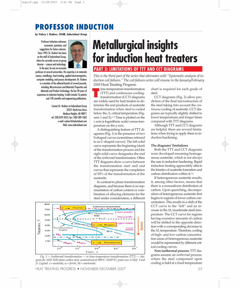
ime-temperature-transformation(TTT) and continuous-cooling-transformation (CCT) diagrams

are widely used by heat treaters to de-termine the end products of austenitetransformation when steel is cooledbelow the A1 critical temperature (Fig-ures 1 and 2).1–5 Time is plotted on thex axis (a logarithmic scale) versus tem-perature on the y axis.

A distinguishing feature of TTT di-agrams (Fig. 1) is the presence of twoS-shaped curves (sometimes referredto as C-shaped curves). The left solidcurve represents the beginning (start)of the transformation process and theright solid curve designates the endof the isothermal transformation. OftenTTT diagrams show a curve betweenthe transformation start and endcurves that represents the completionof 50% of the transformation of theaustenite.

In contrast to phase transformationdiagrams, and because there is no rep-resentation of carbon content or com-bination of alloying elements for thesteel under consideration, a different

chart is required for each grade ofsteel.

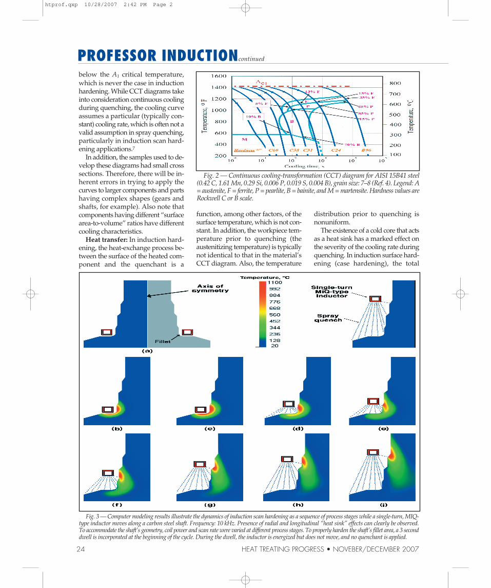
CCT diagrams (Fig. 2) allow pre-diction of the final microstructure ofthe steel taking into account the con-tinuous cooling of austenite. CCT dia-grams are typically slightly shifted tolower temperatures and longer timescompared with TTT diagrams.

Although TTT and CCT diagramsare helpful, there are several limita-tions when trying to apply them to in-duction hardening.

The diagrams’ limitationsBoth the TTT and CCT diagrams

were developed assuming homoge-neous austenite, which is not alwaysthe case in induction hardening. Rapidinduction heating appreciably affectsthe kinetics of austenite formation andcarbon distribution within it.1,6

If heterogeneous austenite results,it, among other factors, means thatthere is a nonuniform distribution ofcarbon. Upon quenching, decompo-sition of heterogeneous austenite firstbegins in regions of lower carbon con-centration. This results in a shift of theCCT curve to the “left” and an in-crease in the Ms (martensite start) tem-perature. The CCT curve for regionshaving excessive amounts of carbonwill be shifted in the opposite direc-tion with a corresponding decrease inthe Ms temperature. Therefore, coolingof high- and low-carbon concentra-tion areas of heterogeneous austenitewould be represented by different crit-ical cooling curves.

Non-isothermal process: TTT dia-grams assume an isothermal process,where the steel component uponcooling is held at a fixed temperature

T

Fig. 1 — Isothermal transformation — or time-temperature-transformation (TTT) — dia-gram for AISI 1020 plain carbon steel, austenitized at 900°C (1650°F); grain size: 6 (Ref. 3 and5). Legend: γ = austenite, α = ferrite, M = martensite.

htprof.qxp 10/28/2007 2:42 PM Page 1

24 HEAT TREATING PROGRESS • NOVEBER/DECEMBER 2007

below the A1 critical temperature,which is never the case in inductionhardening. While CCT diagrams takeinto consideration continuous coolingduring quenching, the cooling curveassumes a particular (typically con-stant) cooling rate, which is often not avalid assumption in spray quenching,particularly in induction scan hard-ening applications.7

In addition, the samples used to de-velop these diagrams had small crosssections. Therefore, there will be in-herent errors in trying to apply thecurves to larger components and partshaving complex shapes (gears andshafts, for example). Also note thatcomponents having different “surfacearea-to-volume” ratios have differentcooling characteristics.

Heat transfer: In induction hard-ening, the heat-exchange process be-tween the surface of the heated com-ponent and the quenchant is a

function, among other factors, of thesurface temperature, which is not con-stant. In addition, the workpiece tem-perature prior to quenching (theaustenitizing temperature) is typicallynot identical to that in the material’sCCT diagram. Also, the temperature

distribution prior to quenching isnonuniform.

The existence of a cold core that actsas a heat sink has a marked effect onthe severity of the cooling rate duringquenching. In induction surface hard-ening (case hardening), the total

PROFESSOR INDUCTIONcontinued

Fig. 2 — Continuous cooling-transformation (CCT) diagram for AISI 15B41 steel(0.42 C, 1.61 Mn, 0.29 Si, 0.006 P, 0.019 S, 0.004 B), grain size: 7–8 (Ref. 4). Legend: A= austenite, F = ferrite, P = pearlite, B = bainite, and M = martensite. Hardness values areRockwell C or B scale.

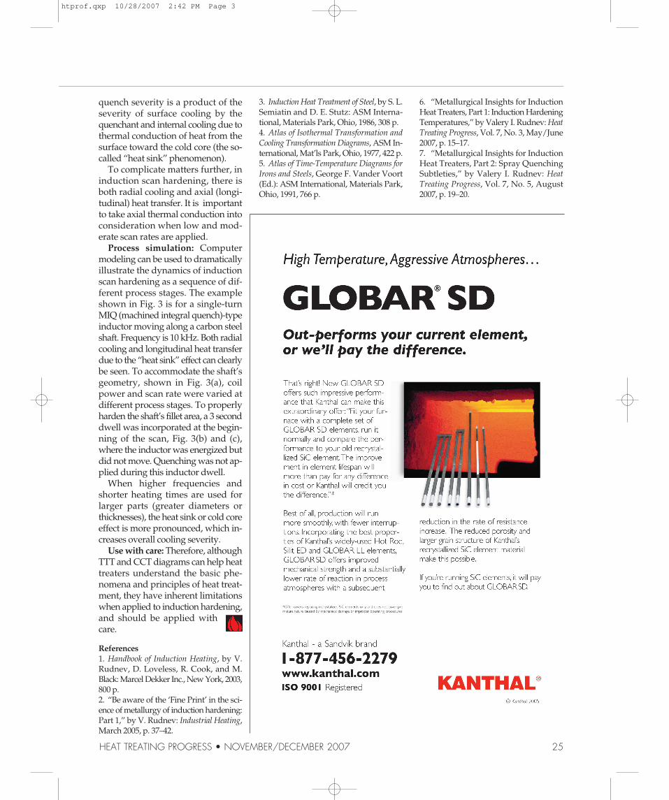
Fig. 3 — Computer modeling results illustrate the dynamics of induction scan hardening as a sequence of process stages while a single-turn, MIQ-type inductor moves along a carbon steel shaft. Frequency: 10 kHz. Presence of radial and longitudinal “heat sink” effects can clearly be observed.To accommodate the shaft’s geometry, coil power and scan rate were varied at different process stages. To properly harden the shaft’s fillet area, a 3 seconddwell is incorporated at the beginning of the cycle. During the dwell, the inductor is energized but does not move, and no quenchant is applied.

htprof.qxp 10/28/2007 2:42 PM Page 2

quench severity is a product of theseverity of surface cooling by thequenchant and internal cooling due tothermal conduction of heat from thesurface toward the cold core (the so-called “heat sink” phenomenon).

To complicate matters further, ininduction scan hardening, there isboth radial cooling and axial (longi-tudinal) heat transfer. It is importantto take axial thermal conduction intoconsideration when low and mod-erate scan rates are applied.

Process simulation: Computermodeling can be used to dramaticallyillustrate the dynamics of inductionscan hardening as a sequence of dif-ferent process stages. The exampleshown in Fig. 3 is for a single-turnMIQ (machined integral quench)-typeinductor moving along a carbon steelshaft. Frequency is 10 kHz. Both radialcooling and longitudinal heat transferdue to the “heat sink” effect can clearlybe seen. To accommodate the shaft’sgeometry, shown in Fig. 3(a), coilpower and scan rate were varied atdifferent process stages. To properlyharden the shaft’s fillet area, a 3 seconddwell was incorporated at the begin-ning of the scan, Fig. 3(b) and (c),where the inductor was energized butdid not move. Quenching was not ap-plied during this inductor dwell.

When higher frequencies andshorter heating times are used forlarger parts (greater diameters orthicknesses), the heat sink or cold coreeffect is more pronounced, which in-creases overall cooling severity.

Use with care: Therefore, althoughTTT and CCT diagrams can help heattreaters understand the basic phe-nomena and principles of heat treat-ment, they have inherent limitationswhen applied to induction hardening,and should be applied withcare.

References1. Handbook of Induction Heating, by V.Rudnev, D. Loveless, R. Cook, and M.Black: Marcel Dekker Inc., New York, 2003,800 p.2. “Be aware of the ‘Fine Print’ in the sci-ence of metallurgy of induction hardening:Part 1,” by V. Rudnev: Industrial Heating,March 2005, p. 37–42.

3. Induction Heat Treatment of Steel, by S. L.Semiatin and D. E. Stutz: ASM Interna-tional, Materials Park, Ohio, 1986, 308 p.4. Atlas of Isothermal Transformation andCooling Transformation Diagrams, ASM In-ternational, Mat’ls Park, Ohio, 1977, 422 p.5. Atlas of Time-Temperature Diagrams forIrons and Steels, George F. Vander Voort(Ed.): ASM International, Materials Park,Ohio, 1991, 766 p.

6. “Metallurgical Insights for InductionHeat Treaters, Part 1: Induction HardeningTemperatures,” by Valery I. Rudnev: HeatTreating Progress, Vol. 7, No. 3, May/June2007, p. 15–17.7. “Metallurgical Insights for InductionHeat Treaters, Part 2: Spray QuenchingSubtleties,” by Valery I. Rudnev: HeatTreating Progress, Vol. 7, No. 5, August2007, p. 19–20.

HEAT TREATING PROGRESS • NOVEMBER/DECEMBER 2007 25

htprof.qxp 10/28/2007 2:42 PM Page 3