METAlab Graph Theoretic General Linear Model Software website: www.nitrc.org/projects/metalab_gtg/ Author: Jeffrey M. Spielberg (jmsp@bu.edu, http://sites.bu.edu/metalab/) Current version: Beta 0.32 (08.26.14) WARNING: This is a beta version. There no known bugs, but only limited testing has been performed. This software comes with no warranty (even the implied warranty of merchantability or fitness for a particular purpose). Therefore, USE AT YOUR OWN RISK!!! Copyleft 2014. Software can be modified and redistributed, but modified, redistributed versions must have the same rights Overview: The main function of this Matlab toolbox is to run a GLM on graph theoretic network properties computed from brain networks. The GLM accepts continuous & categorical between-participant predictors and a categorical within-participant predictor. Significance is determined via non-parametric permutation tests. The toolbox allows testing of both fully connected and thresholded (binarized or not binarized) networks (based on a range of thresholds). Currently, the toolbox works only with undirected matrices (directed matrices and tests of direction/causality will be added in the future). The toolbox also provides a data (pre)processing path for resting state and (block design) task fMRI data. Several options for partialing nuisance signals are included (particularly relevant for resting analyses), including partialing total or local (Jo et al., 2013) white matter signal, partialing the first 5 principal components of white matter/ventricular signal (instead of the means; Muschelli et al., 2014), calculation of Saad et al. (2013)'s GCOR, and the use of Chen et al. (2012)’s GNI method to determine whether global signal partialing is needed. In addition, Power et al. (2014)'s motion scrubbing method and Patel et al. (2014)'s WaveletDespike procedure are available. For task fMRI, the toolbox will compute connectivity matrices for each user-specified condition after dividing up the timeseries by condition. In order to compensate for HDR-related delay, the timeseries’ are first deconvolved (using SPM's method), allowing them to be divided at the actual onset/offset times. Therefore, this method will likely not work for fast event-related designs and may or may not work for slow event-related designs. Even with a block design, extra caution should be used with this method, because we have explored the method only minimally. In-house testing shows that this method produces similar findings to simply assuming a 2-second delay and dividing the timeseries without deconvolution, indicating that the deconvolution process is not introducing any major distortion.

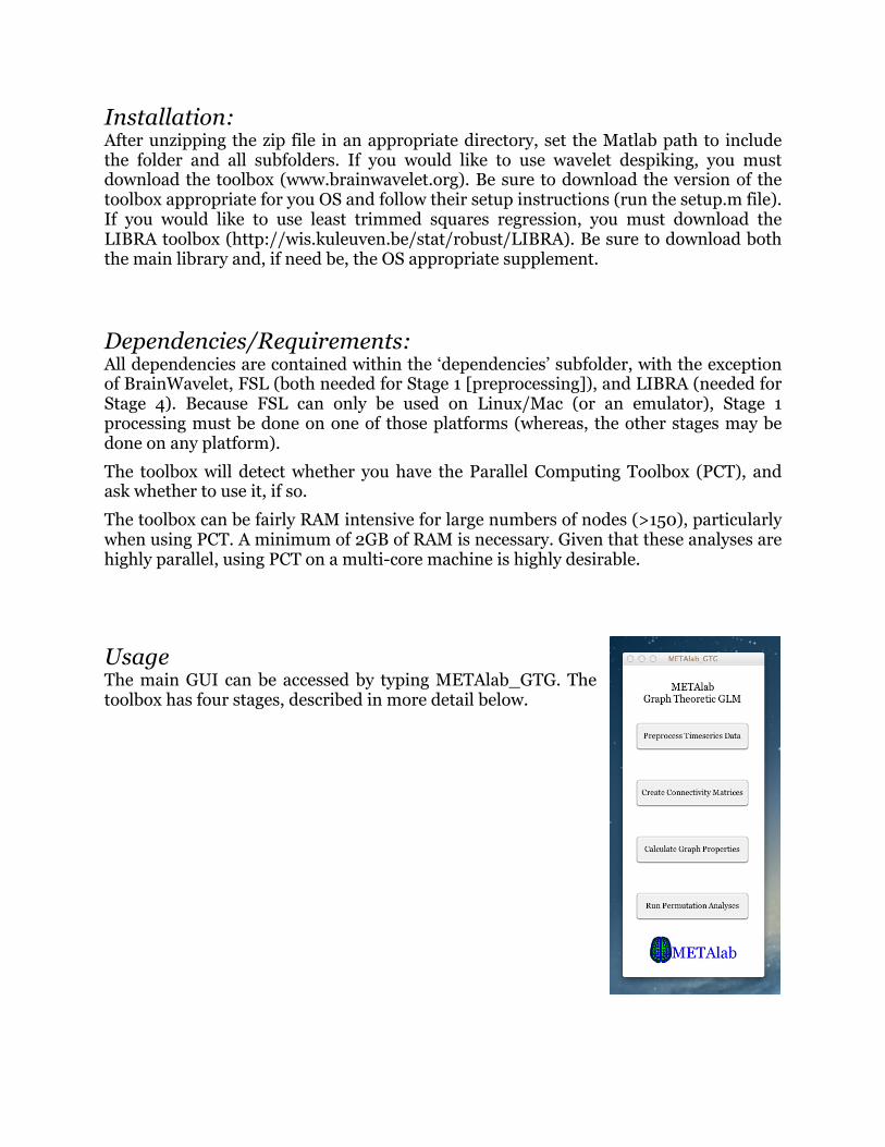
Installation: After unzipping the zip file in an appropriate directory, set the Matlab path to include the folder and all subfolders. If you would like to use wavelet despiking, you must download the toolbox (www.brainwavelet.org). Be sure to download the version of the toolbox appropriate for you OS and follow their setup instructions (run the setup.m file). If you would like to use least trimmed squares regression, you must download the LIBRA toolbox (http://wis.kuleuven.be/stat/robust/LIBRA). Be sure to download both the main library and, if need be, the OS appropriate supplement. Dependencies/Requirements: All dependencies are contained within the ‘dependencies’ subfolder, with the exception of BrainWavelet, FSL (both needed for Stage 1 [preprocessing]), and LIBRA (needed for Stage 4). Because FSL can only be used on Linux/Mac (or an emulator), Stage 1 processing must be done on one of those platforms (whereas, the other stages may be done on any platform). The toolbox will detect whether you have the Parallel Computing Toolbox (PCT), and ask whether to use it, if so. The toolbox can be fairly RAM intensive for large numbers of nodes (>150), particularly when using PCT. A minimum of 2GB of RAM is necessary. Given that these analyses are highly parallel, using PCT on a multi-core machine is highly desirable. Usage The main GUI can be accessed by typing METAlab_GTG. The toolbox has four stages, described in more detail below.

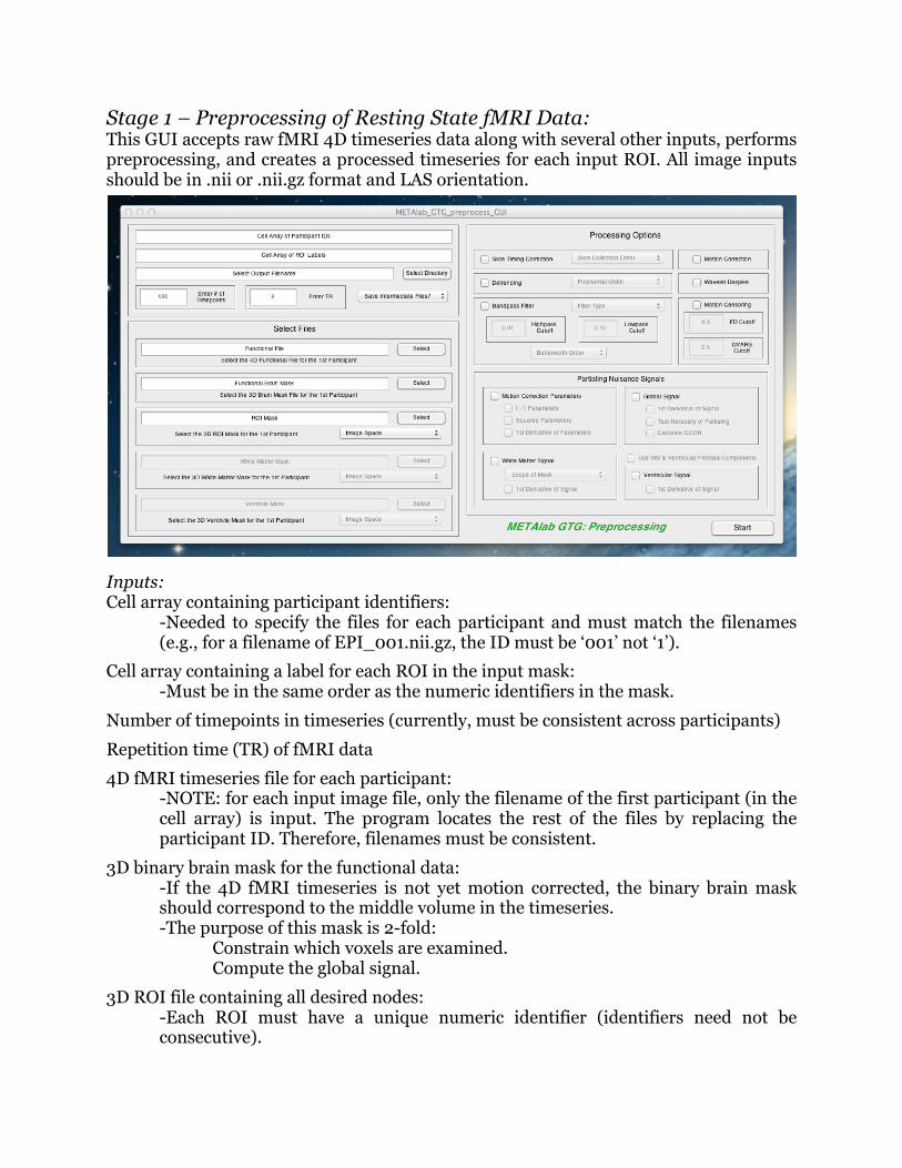
Stage 1 – Preprocessing of Resting State fMRI Data: This GUI accepts raw fMRI 4D timeseries data along with several other inputs, performs preprocessing, and creates a processed timeseries for each input ROI. All image inputs should be in .nii or .nii.gz format and LAS orientation.

Inputs: Cell array containing participant identifiers:

-Needed to specify the files for each participant and must match the filenames (e.g., for a filename of EPI_001.nii.gz, the ID must be ‘001’ not ‘1’).

Cell array containing a label for each ROI in the input mask: -Must be in the same order as the numeric identifiers in the mask.

Number of timepoints in timeseries (currently, must be consistent across participants) Repetition time (TR) of fMRI data 4D fMRI timeseries file for each participant:

-NOTE: for each input image file, only the filename of the first participant (in the cell array) is input. The program locates the rest of the files by replacing the participant ID. Therefore, filenames must be consistent.

3D binary brain mask for the functional data: -If the 4D fMRI timeseries is not yet motion corrected, the binary brain mask should correspond to the middle volume in the timeseries. -The purpose of this mask is 2-fold:

Constrain which voxels are examined. Compute the global signal.

3D ROI file containing all desired nodes: -Each ROI must have a unique numeric identifier (identifiers need not be consecutive).

-NOTE: if the ROI, white matter, and ventricular masks have not yet been transformed into functional space, the user must note the input space and provide the correct transform file (to get to functional space). For standard space to functional, the transform must be a warp file suitable for use with FSL’s FNIRT. For structural space to functional, the transform must be a matrix file suitable for use with FSL’s FLIRT.

3D binary white matter mask: -Optional, only needed if the user wishes to partial white matter signal.

3D binary ventricle mask: -Optional, only needed if the user wishes to partial ventricular signal.

Options (in order of implementation): -Slice timing correction -Motion Correction -Polynomial detrending -Wavelet despiking (using Patel et al. (2014)'s Brain Wavelet Toolbox).

NOTE: despiking is performed with the default parameters. Also, this procedure is likely incompatible with Power et al. (2014)'s motion scrubbing, so only one of these procedures can be used at a time.

-Bandpass filtering Three filter options:

‘Ideal’ filter: This filter is based on that used in REST v. 1.8. This filter achieves complete precision (of cutoff frequency) in the frequency domain at the expense of inducing oscillation in the time domain. Butterworth filter: This filter induces less oscillation in the time domain than the ‘ideal’ filter at the expense of a shallower frequency cutoff. FSL’s nonlinear highpass & Gaussian linear lowpass filter: The non-linearity of the highpass filter may be useful, because non-Gaussianity in lower frequencies may be useful in determining causal direction (Mumford & Ramsey, 2014).

-Partialing of nuisance signals: Motion correction parameters:

-Original 6 parameters. -t - 1 parameters (a la Friston’s autoregressive method). -Squared parameters. -(2nd order) 1st derivative of parameters.

Global signal: -(2nd order) 1st derivative of signal. -Given the controversy surrounding partialing of global signal, two further options are available:

GNI: The user can test the necessity of partialing global signal on a participant specific basis, using Chen et al. (2012)’s GNI method (i.e., global signal is not partialed from data with a GNI > 3). A note of caution should be considered when using this method. Specifically, if GNI correlates with variables of interest, it is possible that partialing global signal for only certain participants may lead to false associations (or mask true effects). Therefore, if this method is used, it is highly recommended that the user ascertain whether global partialing is related to variables of interest.

GCOR: The user can choose to calculate a GCOR (Saad et al., 2013) value for each participant. This value can be used as a covariate in higher-level analyses to reduce bias. See Saad et al. for further details regarding the use of GCOR.

White matter signal: -Default is to extract the signal from the entire white matter mask. However, Jo et al. (2013) suggest that extracting signal from local white matter (i.e., white matter within a 45mm sphere around the current voxel of interest) may help to reduce distance-dependent artifact induced by partialing of the global signal. -(2nd order) 1st derivative of signal -It is possible to remove the first five principal components rather than the mean signal. To do so, click the box labeled 'Use WM & Ventricular Principal Components'.

Ventricular signal: -(2nd order) 1st derivative of signal. -It is possible to remove the first five principal components rather than the mean signal. To do so, click the box labeled 'Use WM & Ventricular Principal Components'.

-Motion scrubbing via Power et al. (2014)'s method: -The FD (frame displacement) cutoff (in mm) must be set. FD is the amount of estimated movement from the previous volume to the current volume. Typical values range from .5mm (liberal) to .2mm (conservative). You should pick a value based on your sample (e.g., if you pick .2mm and this results in throwing out too many participants, you may want to rethink your cutoff or the use of scrubbing in general).

-The DVARS cutoff (in standard deviation units) must be set. DVARS is roughly the change in mean signal from the previous volume to the current volume. The selection of threshold here has the same considerations as FD.

-NOTE: this procedure is likely incompatible with Patel et al. (2014)'s despiking, so only one of these procedures can currently be used at a time.

Outputs: -.mat file containing a structure with processed timeseries for each ROI in the mask, along with numerous other variables used in processing -Logfile Stage 2 – Creation of Connectivity Matrices: This GUI accepts the Stage 1 output and creates connectivity matrices (one per participant/repeated condition). For task fMRI, deconvolution and division by condition are performed, with the option of detrending within block Four measures of association can be used:

-Pearson correlation -Partial correlation

Thought to reflect direct effects to a greater degree. However, this is much less useful in datasets with a very large # of nodes (given the large percentage of variance removed).

-Mutual information Uses the script available in the Functional Connectivity Toolbox

-Robust (bendcorr) Correlation Uses the script available in Corr_toolbox_v2

Outputs: -Output structure containing connectivity matrices for each participant -Logfile

Stage 3 – Calculation of Graph Properties: This stage takes connectivity matrices as input (can, but does not have to be, the Stage 2 output) and calculates graph theoretic properties for each participant/repeated level (to be used as dependent variables in Stage 4).

This stage requires that entries in the connectivity matrices represent connectivity strength, but the measure of connectivity does not matter. In other words, entries could be Pearson correlations (e.g., output from Stage 2) or white matter tract strength (e.g., obtained from diffusion tractography). Therefore, entries do not have to conform to a specific scale. HOWEVER, some properties (e.g., local efficiency) will be calculated incorrectly if entries exceed 1 (or -1). Therefore, if your connectivity matrices contain entries greater than 1 (or < -1), you should rescale them, though ensuring to retain the 0 point (i.e., do not z-score, which will change the 0 point). This can be done by dividing all entries (across participants) by the maximum absolute value in the data or the maximum possible value (e.g., if your measure of strength has a potential max of 2, you could divide by 2 instead of the max in your data, in order to preserve the actual potential range). This stage computes properties for fully-connected and/or (binarized or non-binarized) thresholded networks. For thresholded networks, the toolbox computes properties across a set of density thresholds. The user specifies a desired maximum density (a value of 0.5-0.6 is common) and the desired density step, and the toolbox computes the minimum density. When matrices are 'sparser,' it is possible that the specified maximum density cannot be reached. In this case, the toolbox will use the maximum possible density. Therefore, be sure to check the actual maximum density reached (i.e., out.max_dens_pos, out.max_dens_neg). This may occur, for example, for negative weights in resting data. The minimum density is chosen such that, at the very least, the presence of disconnected networks is not highly correlated with variables of interest (e.g., IVs in Stage 4). Therefore, this computation takes into account variables specified by the user and creates groups of participants by stratifying (e.g., high, medium, low) these variables. Mean networks are created for each (stratification) group, and the minimum

density at which that network remains connected is identified. This is done for each group (across each variable, across all selected variables) and for the overall mean network. Then, the maximum of these minima is chosen as the overall minimum density. After each property is computed (for each threshold), a standardized area under the curve (AUC) is computed for each property, creating one value per property, per participant (or one value for each node/edge, for node/edge specific measures). For both fully connected and thresholded networks, properties will be automatically calculated for positive and negative weights separately (only positive, if absolute value is used). However, it is often the case that an appropriate minimum density cannot be found for negative weights in thresholded matrices, in which case these properties will not be computed. IMPORTANT:  Property  values  for  negative  weights  are  calculated  by  reversing  the  sign  of  the   matrices   and   then   treating   them   the   same   as   the   original   matrices.   Therefore,   you  should  flip  the  signs  for  betas  and  t-­‐vals  from  statistics  calculated  with  these  values  when  interpreting  these  findings.   Inputs: -Connectivity matrices:

-1 matrix per repeated level, per participant. -NOTE: these matrices can have been created in any program and do not have to correspond to resting-state fMRI (e.g., can be diffusion fiber strength). -If repeated-measures tests are desired in Stage 4, the repeated measure should be indexed in the fourth dimension. For example, for 3 repeated levels, 10 participants, and 30 ROIs, the dimensions of the input matrix should be 30 x 30 x 10 x 3. In this stage (3), each level of the repeated factor will be treated independently. Note, Stage 4 uses polynomial contrasts, so arrange the levels of the repeated measure accordingly.

-Cell array containing a label for each ROI -Cell array containing participant identifiers -Variables used to calculate minimum density -Covariates used for calculating minimum density Options: -AUC for Connected Networks:

Because the procedure described above may still leave some disconnected matrices, the user has the option of also computing the AUC on ONLY connected matrices.

-Partial Variables: -The stratified groups can be created using either the original variables or variables that have had the variance associated with the other specified variables (and any covariates) partialed out. -The reason to use partialed variables is because this is the variance that will actually be tested in the GLMs in Stage 4.

-Calculate Properties for Absolute Value of Weights: -By default, properties will be calculated for positive and negative weights separately. However, the user can specify to calculate properties based on the absolute value of network weights, if only the strength of the relationship is of interest.

-Number of Runs for Modularity: -Some properties require a modular structure, which is computed based on the overall mean network (using the Louvain algorithm and then the Fine-tuning algorithm, both from the Brain Connectivity Toolbox). Because modularity calculation is not deterministic (i.e., it depends on the initial start values), this computation is repeated and the organization that maximizes modularity is chosen. Therefore, this value specifies the number of repeated runs (this process is fairly quick, so a large value [5,000-10,000] is recommended).

-Calculate Max Club Size: -Max club size for rich club networks can vary across matrices. Thus, this value can either be computed based on the data or prespecified here.

-Properties for Fully Connected Matrices: -Specify which properties to compute. See the Appendix A for details regarding these properties.

-Properties for Thresholded Matrices: -Specify which properties to compute. See the Appendix A for details regarding these properties.

Output: -Output structure containing graph theoretic properties for each participant

-Properties for fully-connected networks are contained in out_data.fullmat_graph_meas, and for thresholded networks in AUC_thrmat_graph_meas.

-For thresholded matrices, for each property field there is a corresponding field with ‘_numvalsAUC’ appended that indicates the number of values used in computing that particular AUC. This will allow the user to determine whether this varies with variables of interest (which might introduce bias). -If the user specified that AUC should also be computed for only connected networks, the fields corresponding to these values have ‘_nodiscon’ appended.

-The output structure contains other useful values including the modularity

structure (mod_grps) and other values used in processing (serving as a logfile). Stage 4 – Running GLM with Permutation-Based Significance: This stage calculates GLMs with the graph properties computed in Stage 3 as DVs. The user selects IVs and contrasts/F-tests of these IVs (‘contrasts’ is used loosely here to include something like [0 0 1], which would test the significance of the third IV; i.e., contrasts do not have to sum to 0). Continuous & categorical between-participant predictors and a categorical within-participant predictor are accepted.

Testing a single predictor or a contrast between predictors: First, define the design matrix and leave the 'Contrasts' drop-down menu on 'Contrasts'. Next, specify the desired # of contrasts in the box (then hit return or select somewhere else in the GUI). This will create a matrix in the bottom left with a column for each predictor and a row for each contrast. Enter the desired weights for each contrast in the appropriate rows. Testing a between-participant factor: If the factor has only two levels, it should be treated as a single predictor (see above). For more than two levels, first define the design matrix. The factor must be specified in the design matrix by q-1 dummy coded variables (q=#of levels), which can be created in MATLAB using dummyvar (Note: this will create q predictors, so only use the first q-1).

Next, select 'F-tests' from the 'Contrasts' drop-down menu. Next, specify the desired # of F-tests in the box, and enter a 1 in the column associated with each of the dummy coded variables. Testing a within-participant factor: Currently, only a single repeated factor can be specified, with a maximum of eight levels. Additionally, only OLS can be used with repeated-measures. These limitations will be addressed in future releases. Note, the repeated factor must have been specified in Stage 3 (indexed by the 4th dimension, see above). In Stage 4, the toolbox will recognize (based on the Stage 3 output) that there is a repeated measure (and the number of levels). Therefore, nothing different must be done in Stage 4 to test a repeated measure (i.e., specify the desired contrasts/F-tests as described above). Polynomial contrasts are used, and the output will contain (in order): 1) F-test for the between effect (i.e., averaging across levels) 2) F-test for each polynomial contrast (in ascending order, e.g., linear, quadratic, cubic) 3) the omnibus test across (within) levels. The test statistic for the omnibus test will either be a Wilks' Lambda if a contrast is specified for between-participant predictors or an F-test if an F-test is specified for between-participant predictors. Significance is determined via non-parametric permutation tests using the method of Freedman & Lane (1983) (e.g., the same method used in FSL’s Randomise). Because several of the measures are node or edge specific, computation time is greatly increased if ‘Test ALL Nodes’ is specified. Testing all nodes/edges is also problematic in terms of multiple comparisons (i.e., you don’t have to look at all the tests, but it sure is tempting…..). Therefore, we strongly recommend examining only specific nodes/edges at this point. Nodes/edges can be selected based on a priori hypotheses. However, we also highly recommend using Zalesky, Fornito, & Bullmore (2012)’s NBS toolbox to identify specific nodes/edges that vary with IVs of interest.  IMPORTANT:  Property  values  for  negative  weights  are  calculated  by  reversing  the  sign  of  the   matrices   and   then   treating   them   the   same   as   the   original   matrices.   Therefore,   you  should   flip   the   signs   for   betas   and   t-­‐vals   for   tests   of   negative  weights  when   interpreting  these  findings.      Inputs: -Output structure from Stage 3 -IVs of interest Outputs: -Structure containing test statistics (t/F/Wilks' Lambda values, p-values) for each contrast/F-test, for each property selected -Significant effects (at the chosen alpha) are summarized in an output file (<outname>_sig_analyses.txt) and out_data.sig_find  

Appendix  A    NOTE:  The   information   in   this  appendix  has  been  culled   from  a  number  of  sources,  most  notably:    Rubinov,  M.,  Sporns,  O.  (2010).  Complex  network  measures  of  brain  connectivity:  Uses  and  interpretations.  NeuroImage,  52,  1059-­‐1069.    Rubinov  M.,   Sporns   O.   (2011)  Weight-­‐conserving   characterization   of   complex   functional  brain  networks.  NeuroImage,  56,  2068-­‐2079.      Therefore,  most  of  the  credit  should  go  to  these  authors  (but,  all  mistakes  are  mine).        Types of Measures: Functional Segregation: The ability for specialized processing to occur within densely interconnected groups of brain regions. Measures: Clustering Coefficient, Local Efficiency, Transitivity. Functional Integration: The ability to rapidly combine specialized information from distributed brain regions. Measures: Characteristic Path Length, Global Efficiency. Centrality (Influence): The importance of a node (edge) for acting as hubs and facilitating integration. Measures: Degree, (Density for Influence), Diversity Coefficient, Edge Betweeness Centrality, Eigenvector Centrality, K-Coreness Centrality, Node Betweeness Centrality, Node Strength, Pagerank Centrality, Participation Coefficient, Subgraph Centrality, Within-Module Degree Z-Score. Resilience: Network vulnerability to insult. Measures: Assortativity. Measures: Assortativity‡: The correlation between degrees of all nodes on two opposite ends of a link. A measure of resilience. Positive values reflect greater resilience. One value is produced for the entire network. Characteristic Path Length (CPL): The average shortest path between all pairs of nodes. More influenced by shorter paths. A measure of functional integration. Higher values reflect less integration. One value is produced for the entire network.

Clustering Coefficient: The fraction of triangles around a node (the mean across the network is also computed). A measure of functional segregation. Higher values reflect more clustered connectivity. Two outputs, one has one value per node, one describes entire network. Degree: The number of neighbors (edges) of a node. A measure of centrality. Reflects the general importance of a node. Higher values reflect greater importance. Computed only for thresholded networks. One value is produced for each node. Density: Fraction of present connections to possible connections. Similar to the mean degree of all nodes in the network. A measure of influence (centrality on a network scale). Reflects the total “wiring cost” of network. Higher values reflect more interconnected networks. Computed only for thresholded networks. One value is produced for the entire network. Diversity Coefficient: Measures the diversity of intermodular connections (the variance of the weights of edges connected to a node). A measure of centrality. Higher values reflect greater diversity. Computed only for fully connected networks. One value is produced per node. Edge Betweeness Centrality†: The fraction of all the shortest paths in a network that pass through a given edge. A measure of centrality. Higher values suggest that an edge is more important for controlling information flow. One value is produced for each edge. Eigenvector Centrality: The corresponding element of the eigenvector with the largest eigenvalue. A measure of centrality. Higher values suggest that a node is connected to other nodes with high eigenvector centrality. Is more reflective of the global (vs. local) prominence of a node. One value is produced for each node. Global Efficiency: The average inverse shortest path between all pairs of nodes. More influenced by longer paths. A measure of functional integration. Higher values reflect greater integration. One value is produced for the entire network. K-Coreness Centrality: A k-core if the largest subgraph comprising nodes of at least k degree, and the k-coreness of a node is k if the node belongs to the k-core but not the (k+1)-core. A measure of centrality. Higher values reflect greater connectivity to more connected nodes/membership in a relatively more influential network. Computed only for thresholded networks.

One value is produced for each node Local Efficiency: The average inverse shortest path for neighbors of a node (the mean across the network is also computed). Reflects the efficiency of communication among neighbors when a node is removed. A measure of functional segregation. Higher values reflect greater communication. Two outputs, one has one value per node, one describes entire network. Matching Index†: A measure of the similarity between two nodes' connectivity profiles. Higher values reflect greater similarity. One value is produced for each pair of nodes. Node Betweeness Centrality: The fraction of all the shortest paths in a network that pass through a node. A measure of centrality. Higher values suggest that a node is more important for controlling information flow. One value is produced for each node. Node Strength: The sum of the weights connected to a node (the sum across the network is also computed). A measure of centrality. Higher and lower values reflect greater centrality of a node for positive and negative edges, respectively. Computed only for fully connected networks. Two outputs, one has one value per node, one describes entire network. Pagerank Centrality: Similar to eigenvector centrality. A measure of centrality. Higher values suggest greater centrality. Is more reflective of the global (vs. local) prominence of a node. One value is produced for each node. Participation Coefficient: The extent to which a node is connected with nodes outside its module. A measure of centrality. Higher values reflect more between module connectivity. Nodes with a high within module degree z-score but a low participation coefficient are known as provincial hubs and play an important part in facilitating modular segregation. Nodes with both a high within module degree z-score and a high participation coefficient are known as connector hubs and facilitate intermodular communication. One value is produced for each node. Rich Club Networks‡: Reflects the degree to which network hubs tend to be more densely connected among themselves than nodes of a lower degree. One value is produced for each degree size (up to the maximum degree).

Small Worldness: The ratio of clustering coefficient to path length (each normalized by random networks). Higher values reflect more small worldness, and networks high in small worldness have both high integration and segregation. Computed only for thresholded networks. One value is produced for the entire network. Subgraph Centrality: A weighted sum of the closed walks of different lengths in the network starting and ending at the node. Reflects the extent to which a node participates in subgraphs. A measure of centrality. Higher values reflect greater centrality. Computed only for thresholded networks. One value is produced for each node. Transitivity: The (normalized) mean clustering coefficient. A measure of functional segregation. Higher values reflect more clustered connectivity. One value is produced for the entire network. Within-Module Degree Z-Score: The extent to which a node is connected to other nodes in its module. A measure of centrality. Higher values reflect more within module connectivity. Nodes with a high within module degree z-score but a low participation coefficient are known as provincial hubs and play an important part in facilitating modular segregation. Nodes with both a high within module degree z-score and a low participation coefficient are known as connector hubs and facilitate intermodular communication. One value is produced for each node. ‡Calculating this measure depends on the presence of (at least some) zeros; thus, it cannot be calculated when there is non-zero value for all entries of the connectivity matrix; therefore, calculation of this property is automatically turned off when using the absolute value of weights for fully connected matrices †Because a value is produced for each edge, the number of values produced can be quite large and computing/testing can be time consuming.