Musical scale rationalization – a graph-theoreticapproach

Albert GrafInstitute of Musicology, Dept. of Music-InformaticsJohannes Gutenberg-University Mainz, Germany

December 2002

Abstract

While most Western music today uses the well-established equal-tempered 12 tone scale,there are many reasons why composers and music theorists are still interested in “just”scales in which the scale tones are simple integer ratios. Therefore the rationalization ofmusical scales is an important problem in music theory. The first general scale rationaliza-tion algorithm based on a complete enumeration approach was proposed by the influentialcontemporary composer Clarence Barlow. This paper gives a general formulation of theproblem and proves that the problem is NP-complete. The paper also describes new al-gorithms for scale rationalization based on clique search in graphs, and a method to drawrational scales using multidimensional scaling. A scale rationalization and visualizationsoftware based on these algorithms is discussed as well.

1 Introduction

It is a well-known fact that pure musical intervals can be described in terms of simplefrequency ratios, such as 1/1 (the unison or prime), 2/1 (the octave), 3/2 (the perfect fifth)or 5/4 (the major third). It has also been observed that the “pleasantness” or “consonance”of an interval is somehow correlated with the complexity of its frequency ratio. Thus, e.g.,in most contexts the perfect fifth is recognized as the most consonant interval besidesthe prime and the octave. An abundance of different consonance measures have beenproposed, such as Euler’s gradus suavitatis [7], Helmholtz’s harmoniousness measure [9],James Tenney’s harmonic distance [4], Paul Erlich’s harmonic entropy [6] and, last notleast, Clarence Barlow’s harmonicity function [1]. An interesting point about Barlow’sharmonicity function is that it can be employed to rationalize a musical scale. That is,given an arbitrary (not necessarily rational) scale, it is possible to transform the scale intoa rational form in which each scale tone is close to the corresponding tone in the originalscale while keeping to simple integer ratios. For instance, if the input is the usual equal-tempered 12 tone scale then the result will be a just 12 tone scale. The rationalized scalecan then be used, e.g., for compositional purposes or to study harmonic relationships inthe original scale. So this method is valuable for music theorists and composers interestedin just intonation.

Unfortunately, however, scale rationalization is computationally very intensive; as weprove in this paper, the problem is in fact NP-complete. We treat the general case of “sub-additive” consonance measures which yield mathematical metrics on scales. This allows usto both visualize rational scales using multidimensional scaling (another idea proposed byClarence Barlow), and to formulate the scale rationalization problem as a clique problemon an underlying “harmonicity graph”. The latter approach leads to a variety of improvedrationalization algorithms employing variations of the standard clique search algorithm byCarraghan and Pardalos [3], which often help to solve the problem much more efficientlythan with the “brute force” method which requires a complete enumeration of all potentialsolutions. These methods are applicable to a wide range of possible consonance measures,including the ones proposed by Barlow, Euler and Tenney. The algorithms have actu-ally been implemented in a graphical program suitable for experimenting with just andmicrotonal tunings.

The paper is organized as follows. We first give a general definition of subadditiveconsonance measures and the corresponding metrics. We then show how to employ thesefunctions to formulate the scale rationalization problem as a clique problem, prove thatthe problem is NP-complete, and propose some heuristic branch and bound algorithms forsolving the problem. We also discuss how to visualize the harmonicity graph of a scaleusing multidimensional scaling. Finally, we briefly describe a scale rationalization andvisualization software based on our methods, and take a look at some simple examples. Inthe conclusion we summarize our results and point out some directions for further research.

1

2 Harmonicity

The term “consonance” is somewhat troublesome, since it is used to denote several differentphenomena in music theory and psychoacoustics [11]. Hence we adopt Barlow’s terminologyand use the artificial terms harmonicity and disharmonicity throughout this paper.

Barlow’s harmonicities, as well as Euler’s gradus suavitatis and several other consonancemeasures are defined in terms of sums of elementary disharmonicities (called “indigestibili-ties” by Barlow) of the prime factors of a rational interval. In the following we give a genericdefinition which covers all these approaches. So let the prime disharmonicities g(p) > 0for all prime numbers p be given. (We assume throughout that g(p) can be computed inpolynomial time with respect to log p.) We extend g to all positive rational numbers xas follows. If x = pa1

1 pa22 · · · pan

n > 0 is a rational number, where p1 < p2 < · · · < pn arethe prime factors of x and a1, a2, . . . , an their (positive or negative) multiplicities, then thedisharmonicity g(x) of x (with respect to the given prime disharmonicities) is defined as:

g(x) = |a1|g(p1) + |a2|g(p2) + · · ·+ |an|g(pn).

The harmonicity h(x) of x is then defined as the inverse of its disharmonicity, that is,

h(x) = 1/g(x).

Note that, in particular, g(1) = g(1/1) = 0 and hence the unison has infinite harmonic-ity for any given prime disharmonicities. We also remark that the disharmonicity functionis additive for integer arguments, i.e., g(xy) = g(x) + g(y) if x and y are positive integers.Moreover, the disharmonicity of an interval x/y given in its cancelled-down form (i.e., xand y integer, gcd(x, y) = 1), is always the sum of the disharmonicities of the numeratorand the denominator:

g(x/y) = g(x) + g(y) = g(xy).

It is also easy to see that in the general case, for arbitrary rational values x, y > 0, thedisharmonicity function is subadditive:

g(xy) ≤ g(x) + g(y).

Using the generic definition above, we can obtain various different harmonicity measuressuch as Barlow’s disharmonicities and Euler’s gradus function by just plugging in suitableprime disharmonicities. For instance:

• Barlow disharmonicities: gB(p) = 2(p− 1)2/p

• Euler disharmonicities: gE(p) = p− 1

The Barlow and Euler disharmonicities for some common intervals are shown in Fig.1. (The meaning of the “cent” values is explained below.) Note that the factor 2 in thedefinition of the Barlow disharmonicities is just a normalization factor which makes theoctave 2/1 have a value of 1. We also remark that Euler’s original definition of the gradus

2

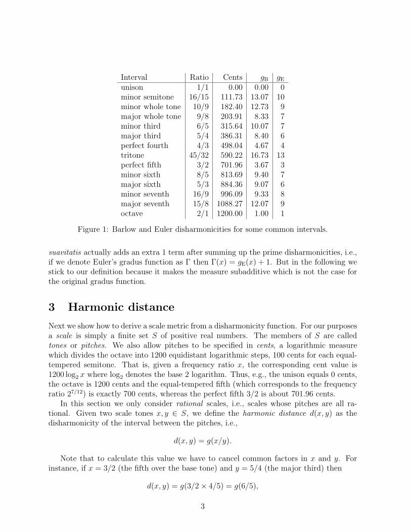
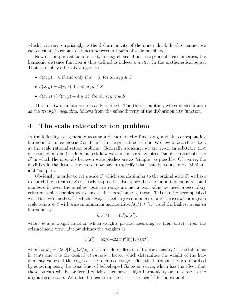
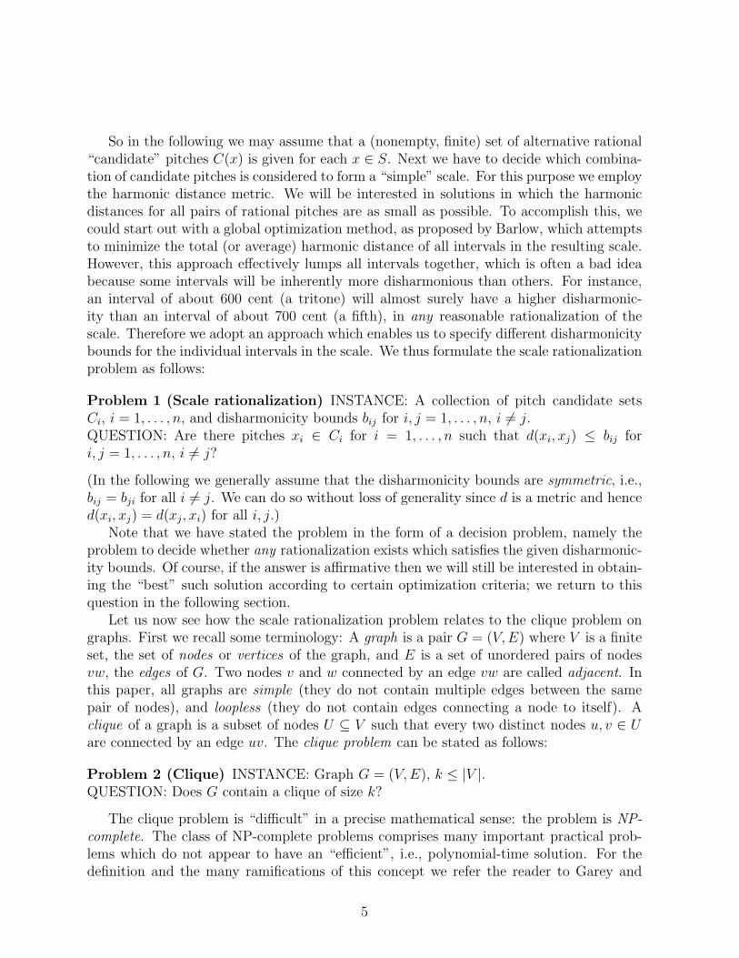
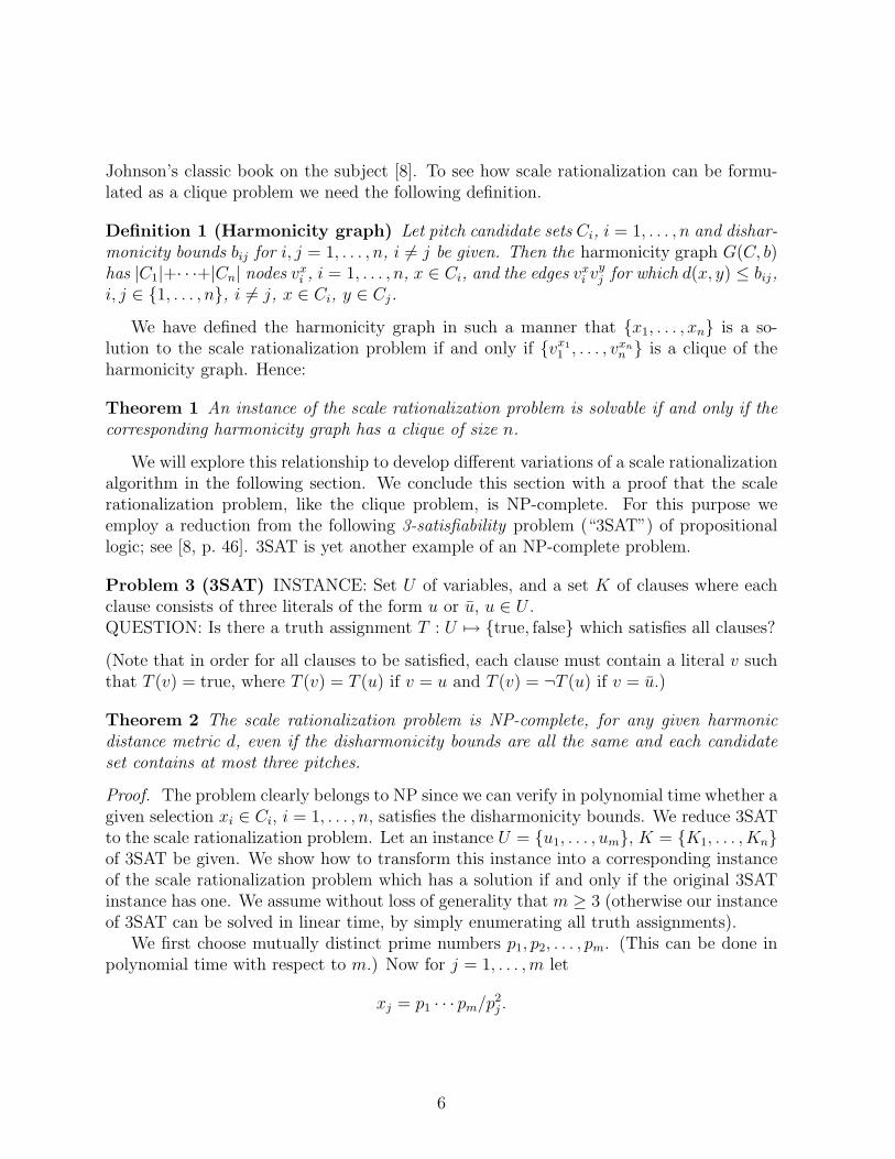
Interval Ratio Cents gB gE

unison 1/1 0.00 0.00 0minor semitone 16/15 111.73 13.07 10minor whole tone 10/9 182.40 12.73 9major whole tone 9/8 203.91 8.33 7minor third 6/5 315.64 10.07 7major third 5/4 386.31 8.40 6perfect fourth 4/3 498.04 4.67 4tritone 45/32 590.22 16.73 13perfect fifth 3/2 701.96 3.67 3minor sixth 8/5 813.69 9.40 7major sixth 5/3 884.36 9.07 6minor seventh 16/9 996.09 9.33 8major seventh 15/8 1088.27 12.07 9octave 2/1 1200.00 1.00 1

Figure 1: Barlow and Euler disharmonicities for some common intervals.

suavitatis actually adds an extra 1 term after summing up the prime disharmonicities, i.e.,if we denote Euler’s gradus function as Γ then Γ(x) = gE(x) + 1. But in the following westick to our definition because it makes the measure subadditive which is not the case forthe original gradus function.

3 Harmonic distance

Next we show how to derive a scale metric from a disharmonicity function. For our purposesa scale is simply a finite set S of positive real numbers. The members of S are calledtones or pitches. We also allow pitches to be specified in cents, a logarithmic measurewhich divides the octave into 1200 equidistant logarithmic steps, 100 cents for each equal-tempered semitone. That is, given a frequency ratio x, the corresponding cent value is1200 log2 x where log2 denotes the base 2 logarithm. Thus, e.g., the unison equals 0 cents,the octave is 1200 cents and the equal-tempered fifth (which corresponds to the frequencyratio 27/12) is exactly 700 cents, whereas the perfect fifth 3/2 is about 701.96 cents.

In this section we only consider rational scales, i.e., scales whose pitches are all ra-tional. Given two scale tones x, y ∈ S, we define the harmonic distance d(x, y) as thedisharmonicity of the interval between the pitches, i.e.,

d(x, y) = g(x/y).

Note that to calculate this value we have to cancel common factors in x and y. Forinstance, if x = 3/2 (the fifth over the base tone) and y = 5/4 (the major third) then

d(x, y) = g(3/2× 4/5) = g(6/5),

3

which, not very surprisingly, is the disharmonicity of the minor third. In this manner wecan calculate harmonic distances between all pairs of scale members.

Now it is important to note that, for any choice of positive prime disharmonicities, theharmonic distance function d thus defined is indeed a metric in the mathematical sense.That is, it obeys the following rules:

• d(x, y) = 0 if and only if x = y, for all x, y ∈ S

• d(x, y) = d(y, x), for all x, y ∈ S

• d(x, z) ≤ d(x, y) + d(y, z), for all x, y, z ∈ S

The first two conditions are easily verified. The third condition, which is also knownas the triangle inequality, follows from the subadditivity of the disharmonicity function.

4 The scale rationalization problem

In the following we generally assume a disharmonicity function g and the correspondingharmonic distance metric d as defined in the preceding section. We now take a closer lookat the scale rationalization problem. Generally speaking, we are given an arbitrary (notnecessarily rational) scale S and ask how we can transform S into a “similar” rational scaleS ′ in which the intervals between scale pitches are as “simple” as possible. Of course, thedevil lies in the details, and so we now have to specify what exactly we mean by “similar”and “simple”.

Obviously, in order to get a scale S ′ which sounds similar to the orginal scale S, we haveto match the pitches of S as closely as possible. But since there are infinitely many rationalnumbers in even the smallest positive range around a real value we need a secondarycriterion which enables us to choose the “best” among those. This can be accomplishedwith Barlow’s method [1] which always selects a given number of alternatives x′ for a givenscale tone x ∈ S with a given minimum harmonicity, h(x′) ≥ hmin, and the highest weightedharmonicity

hw(x′) = w(x′)h(x′),

where w is a weight function which weights pitches according to their offsets from theoriginal scale tone. Barlow defines the weights as

w(x′) = exp(−∆(x′)2 ln(1/a)/t2),

where ∆(x′) = 1200| log2(x′/x)| is the absolute offset of x′ from x in cents, t is the tolerance

in cents and a is the desired attenuation factor which determines the weight of the har-monicity values at the edges of the tolerance range. Thus the harmonicities are modifiedby superimposing the usual kind of bell-shaped Gaussian curve, which has the effect thatthose pitches will be preferred which either have a high harmonicity or are close to theoriginal scale tone. We refer the reader to the cited reference [1] for an example.

4

So in the following we may assume that a (nonempty, finite) set of alternative rational“candidate” pitches C(x) is given for each x ∈ S. Next we have to decide which combina-tion of candidate pitches is considered to form a “simple” scale. For this purpose we employthe harmonic distance metric. We will be interested in solutions in which the harmonicdistances for all pairs of rational pitches are as small as possible. To accomplish this, wecould start out with a global optimization method, as proposed by Barlow, which attemptsto minimize the total (or average) harmonic distance of all intervals in the resulting scale.However, this approach effectively lumps all intervals together, which is often a bad ideabecause some intervals will be inherently more disharmonious than others. For instance,an interval of about 600 cent (a tritone) will almost surely have a higher disharmonic-ity than an interval of about 700 cent (a fifth), in any reasonable rationalization of thescale. Therefore we adopt an approach which enables us to specify different disharmonicitybounds for the individual intervals in the scale. We thus formulate the scale rationalizationproblem as follows:

Problem 1 (Scale rationalization) INSTANCE: A collection of pitch candidate setsCi, i = 1, . . . , n, and disharmonicity bounds bij for i, j = 1, . . . , n, i 6= j.QUESTION: Are there pitches xi ∈ Ci for i = 1, . . . , n such that d(xi, xj) ≤ bij fori, j = 1, . . . , n, i 6= j?

(In the following we generally assume that the disharmonicity bounds are symmetric, i.e.,bij = bji for all i 6= j. We can do so without loss of generality since d is a metric and henced(xi, xj) = d(xj, xi) for all i, j.)

Note that we have stated the problem in the form of a decision problem, namely theproblem to decide whether any rationalization exists which satisfies the given disharmonic-ity bounds. Of course, if the answer is affirmative then we will still be interested in obtain-ing the “best” such solution according to certain optimization criteria; we return to thisquestion in the following section.

Let us now see how the scale rationalization problem relates to the clique problem ongraphs. First we recall some terminology: A graph is a pair G = (V, E) where V is a finiteset, the set of nodes or vertices of the graph, and E is a set of unordered pairs of nodesvw, the edges of G. Two nodes v and w connected by an edge vw are called adjacent. Inthis paper, all graphs are simple (they do not contain multiple edges between the samepair of nodes), and loopless (they do not contain edges connecting a node to itself). Aclique of a graph is a subset of nodes U ⊆ V such that every two distinct nodes u, v ∈ Uare connected by an edge uv. The clique problem can be stated as follows:

Problem 2 (Clique) INSTANCE: Graph G = (V, E), k ≤ |V |.QUESTION: Does G contain a clique of size k?

The clique problem is “difficult” in a precise mathematical sense: the problem is NP-complete. The class of NP-complete problems comprises many important practical prob-lems which do not appear to have an “efficient”, i.e., polynomial-time solution. For thedefinition and the many ramifications of this concept we refer the reader to Garey and

5

Johnson’s classic book on the subject [8]. To see how scale rationalization can be formu-lated as a clique problem we need the following definition.

Definition 1 (Harmonicity graph) Let pitch candidate sets Ci, i = 1, . . . , n and dishar-monicity bounds bij for i, j = 1, . . . , n, i 6= j be given. Then the harmonicity graph G(C, b)has |C1|+· · ·+|Cn| nodes vx

i , i = 1, . . . , n, x ∈ Ci, and the edges vxi vy

j for which d(x, y) ≤ bij,i, j ∈ {1, . . . , n}, i 6= j, x ∈ Ci, y ∈ Cj.

We have defined the harmonicity graph in such a manner that {x1, . . . , xn} is a so-lution to the scale rationalization problem if and only if {vx1

1 , . . . , vxnn } is a clique of the

harmonicity graph. Hence:

Theorem 1 An instance of the scale rationalization problem is solvable if and only if thecorresponding harmonicity graph has a clique of size n.

We will explore this relationship to develop different variations of a scale rationalizationalgorithm in the following section. We conclude this section with a proof that the scalerationalization problem, like the clique problem, is NP-complete. For this purpose weemploy a reduction from the following 3-satisfiability problem (“3SAT”) of propositionallogic; see [8, p. 46]. 3SAT is yet another example of an NP-complete problem.

Problem 3 (3SAT) INSTANCE: Set U of variables, and a set K of clauses where eachclause consists of three literals of the form u or u, u ∈ U .QUESTION: Is there a truth assignment T : U 7→ {true, false} which satisfies all clauses?

(Note that in order for all clauses to be satisfied, each clause must contain a literal v suchthat T (v) = true, where T (v) = T (u) if v = u and T (v) = ¬T (u) if v = u.)

Theorem 2 The scale rationalization problem is NP-complete, for any given harmonicdistance metric d, even if the disharmonicity bounds are all the same and each candidateset contains at most three pitches.

Proof. The problem clearly belongs to NP since we can verify in polynomial time whether agiven selection xi ∈ Ci, i = 1, . . . , n, satisfies the disharmonicity bounds. We reduce 3SATto the scale rationalization problem. Let an instance U = {u1, . . . , um}, K = {K1, . . . , Kn}of 3SAT be given. We show how to transform this instance into a corresponding instanceof the scale rationalization problem which has a solution if and only if the original 3SATinstance has one. We assume without loss of generality that m ≥ 3 (otherwise our instanceof 3SAT can be solved in linear time, by simply enumerating all truth assignments).

We first choose mutually distinct prime numbers p1, p2, . . . , pm. (This can be done inpolynomial time with respect to m.) Now for j = 1, . . . ,m let

xj = p1 · · · pm/p2j .

6

Then for each j, j1, j2 ∈ {1, . . . ,m}, j1 6= j2, we have:

g(x2j) = 2

m∑j=1

g(pj) g(xj/xj) = 0

g(xj1xj2) = 2∑

j 6=j1,j2

g(pj) g(xj1/xj2) = 2g(pj1) + 2g(pj2)

Thus, since m ≥ 3, it is possible to choose a bound B such that g(xj1xj2) > B ifj1 = j2 and g(xj1xj2), g(xj1/xj2) ≤ B otherwise. We now construct an instance of the scalerationalization problem as follows. For each clause Ki let Ci be the set of pitches xj forwhich uj ∈ Ki and pitches 1/xj for which uj ∈ Ki. Furthermore, let bi1i2 = B for alli1, i2 ∈ {1, . . . , n}, i1 6= i2. Now it is easy to verify that S = {y1, . . . , yn}, yi ∈ Ci, is asolution for the scale rationalization instance if and only if T is a satisfying truth assignmentfor the 3SAT instance, where T (uj) = true iff xj ∈ S, j = 1, . . . ,m. Conversely, if T isa satisfying truth assignment then we can pick a literal vji

∈ Ki ∩ {uji, uji

} such thatT (vji

) = true for i = 1, . . . , n. We then obtain a solution S = {y1, . . . , yn} for the scalerationalization instance, where yi = xji

if vji= uji

and yi = 1/xjiotherwise. q.e.d.

5 Scale rationalization algorithms

Using the relationship between scale rationalization and the clique problem established inthe previous section, we now show how to solve the rationalization problem with Carraghanand Pardalos’ branch and bound procedure for enumerating cliques in a graph [3]. Thebasic algorithm is shown in Fig. 2. The algorithm starts out with an initial solution C(the empty clique) and the set V of all nodes of G. It then adds nodes from V to thecurrent clique C, one at a time, checks whether the new configuration can still lead to aclique of the desired size, and invokes itself recursively on the new partial solution. Theinvariant maintained during execution of the algorithm is the fact that C always is a cliqueof G and the current set of candidate nodes V consists of all nodes which are adjacent toall nodes in C. The algorithm terminates when all cliques have been enumerated. (In aconcrete implementation we will of course stop the algorithm as soon as the desired numberof cliques has been produced.)

If you compare the above algorithm to the original one in [3], you will notice some slightmodifications. First, the node selection strategy (step 7 of the algorithm) is adaptablerather than using a fixed node order determined before execution; this allows us to applydifferent search strategies as described below. Second, the recursion is terminated as soonas a clique of the given size is found; this accounts for the fact that we know in advancehow large our cliques must be.

To apply the algorithm to the scale rationalization problem, it is invoked on the har-monicity graph for the given problem instance (cf. Definition 1) and with the desired cliquesize k = n. If we just want to take a quick look at some (not necessarily optimal) solutions,the algorithm can be run until the desired number of alternative solutions is obtained. But

7

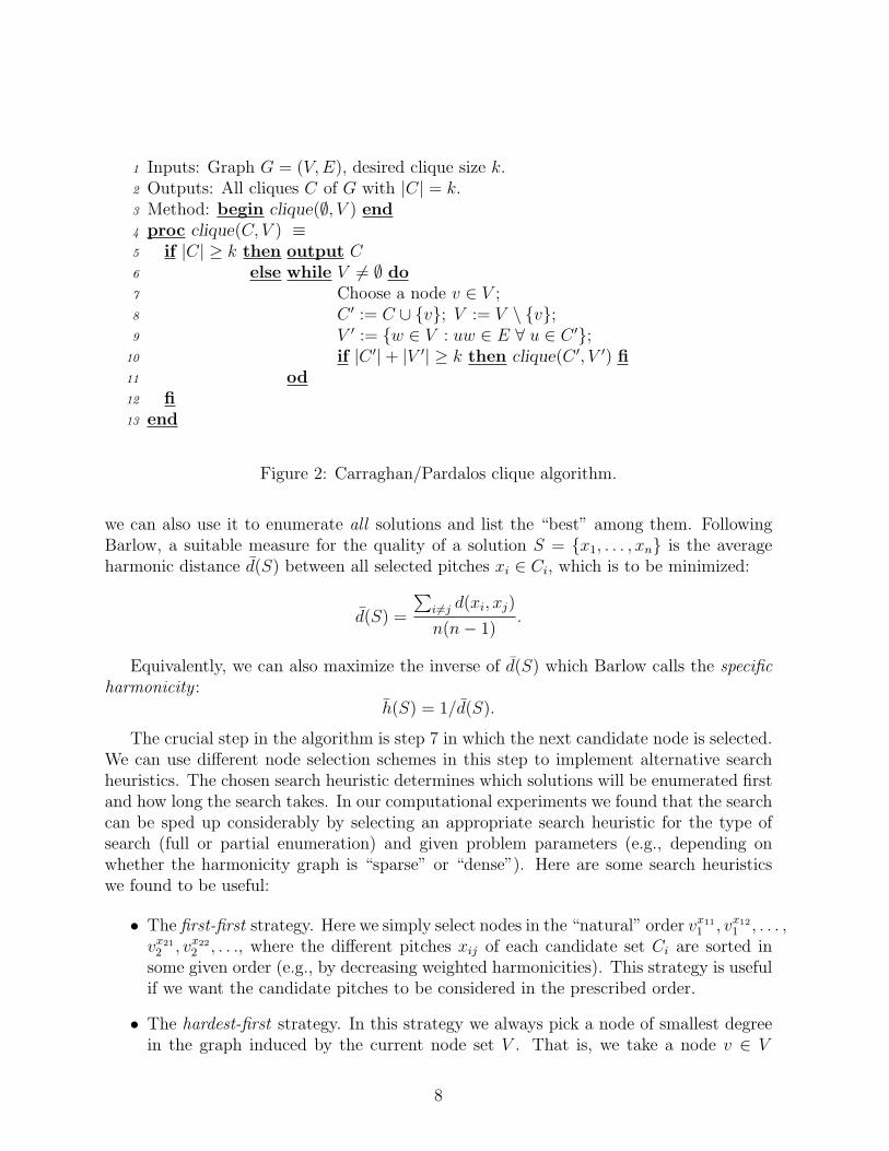
1 Inputs: Graph G = (V, E), desired clique size k.2 Outputs: All cliques C of G with |C| = k.3 Method: begin clique(∅, V ) end4 proc clique(C, V ) ≡5 if |C| ≥ k then output C6 else while V 6= ∅ do7 Choose a node v ∈ V ;8 C ′ := C ∪ {v}; V := V \ {v};9 V ′ := {w ∈ V : uw ∈ E ∀ u ∈ C ′};

10 if |C ′|+ |V ′| ≥ k then clique(C ′, V ′) fi11 od12 fi13 end

Figure 2: Carraghan/Pardalos clique algorithm.

we can also use it to enumerate all solutions and list the “best” among them. FollowingBarlow, a suitable measure for the quality of a solution S = {x1, . . . , xn} is the averageharmonic distance d(S) between all selected pitches xi ∈ Ci, which is to be minimized:

d(S) =

∑i6=j d(xi, xj)

n(n− 1).

Equivalently, we can also maximize the inverse of d(S) which Barlow calls the specificharmonicity :

h(S) = 1/d(S).

The crucial step in the algorithm is step 7 in which the next candidate node is selected.We can use different node selection schemes in this step to implement alternative searchheuristics. The chosen search heuristic determines which solutions will be enumerated firstand how long the search takes. In our computational experiments we found that the searchcan be sped up considerably by selecting an appropriate search heuristic for the type ofsearch (full or partial enumeration) and given problem parameters (e.g., depending onwhether the harmonicity graph is “sparse” or “dense”). Here are some search heuristicswe found to be useful:

• The first-first strategy. Here we simply select nodes in the “natural” order vx111 , vx12

1 , . . . ,vx21

2 , vx222 , . . ., where the different pitches xij of each candidate set Ci are sorted in

some given order (e.g., by decreasing weighted harmonicities). This strategy is usefulif we want the candidate pitches to be considered in the prescribed order.

• The hardest-first strategy. In this strategy we always pick a node of smallest degreein the graph induced by the current node set V . That is, we take a node v ∈ V

8

which minimizes the value |{w ∈ V : vw ∈ E}|. The rationale behind this strategyis that we want to do “the hardest nodes first” in order to reduce the number ofalternatives to consider in later stages of the algorithm. It has been observed byCarraghan and Pardalos that this approach in fact tends to reduce the overall runningtime if the input graph is dense. Thus this strategy is appropriate if there are many“harmonious” intervals in the harmonicity graph. We also found this strategy helpfulwhen enumerating all solutions in order to find an optimal solution.

• The random-first strategy. Here we always select the next node at random (eachnode v ∈ V is selected with the same probability). This strategy is useful if onewants to have a quick look at the average solution quality.

• The best-first strategy. In this strategy we always select a node v ∈ V which mini-mizes

∑vw∈Ew∈C d(v, w) where d(v, w) denotes the harmonic distance between the pitches

represented by the nodes v and w. This strategy tends to enumerate solutions firstwhich have a lower average harmonic distance; it effectively turns the algorithm into a“greedy” heuristic. This is useful if we want to find some “good” (but not necessarilyoptimal) solutions quickly.

Note that all described variations of the algorithm take exponential time in the worstcase. As we have pointed out in the previous section, the scale rationalization problemis NP-complete already in its decision form and hence one cannot hope for a polynomial-time solution. However, we have found the procedures based on the Carraghan/Pardalosalgorithm to be a good solution method for the problem, since they enable us to experimentwith different search strategies and algorithm parameters until a good solution is obtainedin a reasonable amount of time. The algorithm seems to be practical for the usual kindsof scales composers work with, which rarely have more than a few dozen pitches.

We remark that other, more advanced algorithmic approaches to the scale rational-ization problem seem possible. As we point out in the following section, one can often“embed” scale metrics in the Euclidean plane or space. This fact could lead to more effi-cient algorithms for some special cases of the problem, by exploiting geometric structure.For instance, it is known that for a certain class of “geometric” graphs, namely the “unitdisk” graphs, the clique problem can actually be solved in polynomial time using bipartitematching techniques [5]. Geometric graphs have their edges defined in terms of Euclideandistances between the nodes, just like we defined the edges of the harmonicity graphs interms of harmonic distances. Thus it might be possible to apply similar techniques to solvesome special cases of the scale rationalization problem as well.

6 Drawing a scale

We now discuss how to visualize a rational scale by drawing its harmonicity graph in 2-or 3-dimensional space in such a manner that the visible (Euclidean) distances betweenthe scale tones provide a good approximation for the actual harmonic distances. (The

9

harmonicity graph G(S) of a rational scale S = {x1, . . . , xn} is defined analogously toDefinition 1, but now there is only one node vi for each scale tone xi.) Such visualizationsmake it easy to spot the harmonic relationships inside a scale and to compare differentrationalizations of a scale by just taking a look at the corresponding pictures.

The method we employ for this purpose is called multidimensional scaling (henceforthabbreviated as “MDS”). Whenever we have a metric d on a finite set S = {x1, . . . , xn},MDS can be used to embed the members of the set into m-dimensional Euclidean space, byassigning a point ui to each xi ∈ S such that the Euclidean distances d2(ui, uj) = ||ui − uj||2match the metric distances d(xi, xj) as closely as possible. Of course, if we want to drawa real picture, say, on a computer screen, we better find an embedding in low-dimensionalspace. Hence for our purposes we concentrate on 2- and 3-dimensional embeddings. Inour software we also perform a principle axis rotation of the resulting embedding, so thatthe coordinates with the greatest amount of variation are on the x and y axes. Anotherpoint that deserves mentioning is that the embeddings produced with MDS are usuallynot determined uniquely; depending on the choice of parameters, the MDS algorithm mayproduce distinct embeddings which correspond to different local minima of the “stress”function explained below.

MDS is routinely used in the social sciences to analyze statistical data involving sim-ilarity measurements. A fortunate consequence of this situation is that an abundance ofdifferent MDS methods is readily available, like, e.g., Torgerson’s “classical” algorithm [12]and Kruskal’s gradient method [10]. The method we mainly employ in our software isa modern MDS algorithm due to De Leeuw and Heiser, called “SMACOF” (the curiousacronym stands for “scaling by majorizing a convex function”), see [2] for details. Thisalgorithm, like most others, attempts to minimize the so-called stress of the embedding,which is a measure for the error in the representation, defined as:

σ =∑i<j

(d2(ui, uj)− d(xi, xj))2.

If the stress is zero then the embedding provides a perfect visualization. This is rarelyachieved since many interesting metrics are not Euclidean at all (this condition can bechecked using Torgerson’s algorithm), and even if a metric is Euclidean then it mightnot be perfectly embeddable in low-dimensional space. This also happens with harmonicdistance metrics, but we have found that the embeddings produced for many interestingscales provide fairly good representations of the harmonic distances, at least for the Barlowand Euler metrics (we have not tried other metrics with a substantial number of examplesyet). To determine the relative error in the representation one usually works with a relativekind of stress measure, called stress-1, which is defined as the ratio between σ and the totalof the squared metric values,

∑i<j d(xi, xj)

2. A rule of thumb says that an MDS solutionis acceptable if the stress-1 value, as a percentage, does not exceed some 10%.

As an example, Fig. 3 shows the Barlow harmonicity graph of an Indian shruti scalewhich exhibits a fairly regular structure. The edges of the graph are for a harmonicitythreshold of 0.1 (i.e., edges are shown for all intervals with a maximum Barlow dishar-monicity of 10). The picture makes it easy to spot the chains of fifths in the scale, as well

10

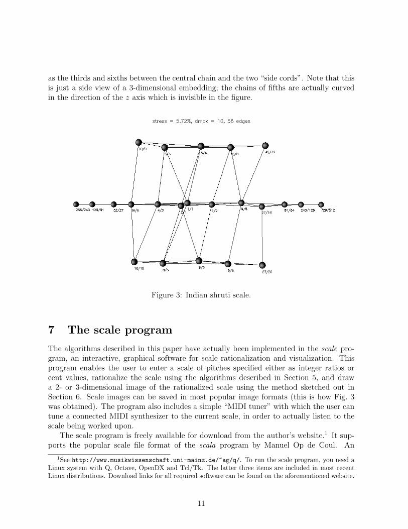
as the thirds and sixths between the central chain and the two “side cords”. Note that thisis just a side view of a 3-dimensional embedding; the chains of fifths are actually curvedin the direction of the z axis which is invisible in the figure.

Figure 3: Indian shruti scale.

7 The scale program

The algorithms described in this paper have actually been implemented in the scale pro-gram, an interactive, graphical software for scale rationalization and visualization. Thisprogram enables the user to enter a scale of pitches specified either as integer ratios orcent values, rationalize the scale using the algorithms described in Section 5, and drawa 2- or 3-dimensional image of the rationalized scale using the method sketched out inSection 6. Scale images can be saved in most popular image formats (this is how Fig. 3was obtained). The program also includes a simple “MIDI tuner” with which the user cantune a connected MIDI synthesizer to the current scale, in order to actually listen to thescale being worked upon.

The scale program is freely available for download from the author’s website.1 It sup-ports the popular scale file format of the scala program by Manuel Op de Coul. An

1See http://www.musikwissenschaft.uni-mainz.de/~ag/q/. To run the scale program, you need aLinux system with Q, Octave, OpenDX and Tcl/Tk. The latter three items are included in most recentLinux distributions. Download links for all required software can be found on the aforementioned website.

11

extensive archive with more than 2800 different scales in scala format is available from Opde Coul’s website.2

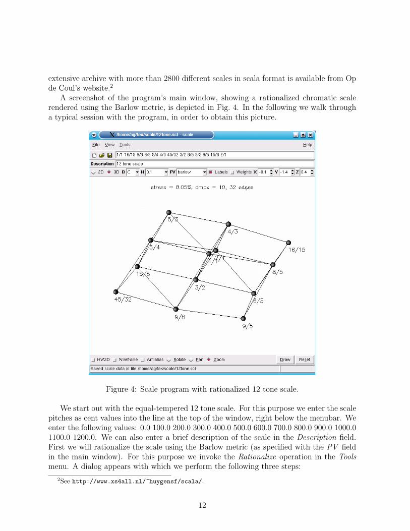
A screenshot of the program’s main window, showing a rationalized chromatic scalerendered using the Barlow metric, is depicted in Fig. 4. In the following we walk througha typical session with the program, in order to obtain this picture.

Figure 4: Scale program with rationalized 12 tone scale.

We start out with the equal-tempered 12 tone scale. For this purpose we enter the scalepitches as cent values into the line at the top of the window, right below the menubar. Weenter the following values: 0.0 100.0 200.0 300.0 400.0 500.0 600.0 700.0 800.0 900.0 1000.01100.0 1200.0. We can also enter a brief description of the scale in the Description field.First we will rationalize the scale using the Barlow metric (as specified with the PV fieldin the main window). For this purpose we invoke the Rationalize operation in the Toolsmenu. A dialog appears with which we perform the following three steps:

2See http://www.xs4all.nl/~huygensf/scala/.

12

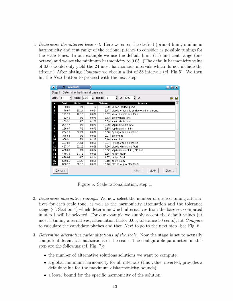
1. Determine the interval base set. Here we enter the desired (prime) limit, minimumharmonicity and cent range of the rational pitches to consider as possible tunings forthe scale tones. In our example we use the default limit (11) and cent range (oneoctave) and we set the minimum harmonicity to 0.05. (The default harmonicity valueof 0.06 would only yield the 24 most harmonious intervals which do not include thetritone.) After hitting Compute we obtain a list of 38 intervals (cf. Fig 5). We thenhit the Next button to proceed with the next step.

Figure 5: Scale rationalization, step 1.

2. Determine alternative tunings. We now select the number of desired tuning alterna-tives for each scale tone, as well as the harmonicity attenuation and the tolerancerange (cf. Section 4) which determine which alternatives from the base set computedin step 1 will be selected. For our example we simply accept the default values (atmost 3 tuning alternatives, attenuation factor 0.05, tolerance 50 cents), hit Computeto calculate the candidate pitches and then Next to go to the next step. See Fig. 6.

3. Determine alternative rationalizations of the scale. Now the stage is set to actuallycompute different rationalizations of the scale. The configurable parameters in thisstep are the following (cf. Fig. 7):

• the number of alternative solutions solutions we want to compute;

• a global minimum harmonicity for all intervals (this value, inverted, provides adefault value for the maximum disharmonicity bounds);

• a lower bound for the specific harmonicity of the solution;

13

Figure 6: Scale rationalization, step 2.

Figure 7: Scale rationalization, step 3.

14

• the type of algorithm and search heuristic to invoke.

For a first run, we can simply keep the default settings which will invoke the scalerationalization algorithm described in Section 5 to compute the first three solutions usingthe “first-first” strategy. A short while after hitting the Compute button the solutions willbe displayed. Except for the first solution with a specific harmonicity of about 0.08, thesesolutions are not very good, so let’s try the “best-first” strategy instead (we select Bestin the Heur field and push Compute again). Now we already have two solutions with aspecific harmonicity of 0.08.

But we are still not satisfied; now we want to go for a (nearly) optimal solution, byselecting the Best algorithm in the Alg field. This requires some careful tuning of thealgorithm parameters since the real optimum might take hours to compute. Taking a lookat the best solutions from the second run we see that all these solutions have a minimuminterval harmonicity (the values in parentheses behind the specific harmonicities in eachcolumn header) of more than 0.033. So we decide to increase the value in the Hmin field to0.033; this will reduce the number of edges in the harmonicity graph and hopefully speedup the algorithm.

Figure 8: Scale rationalization, step 3, detail settings.

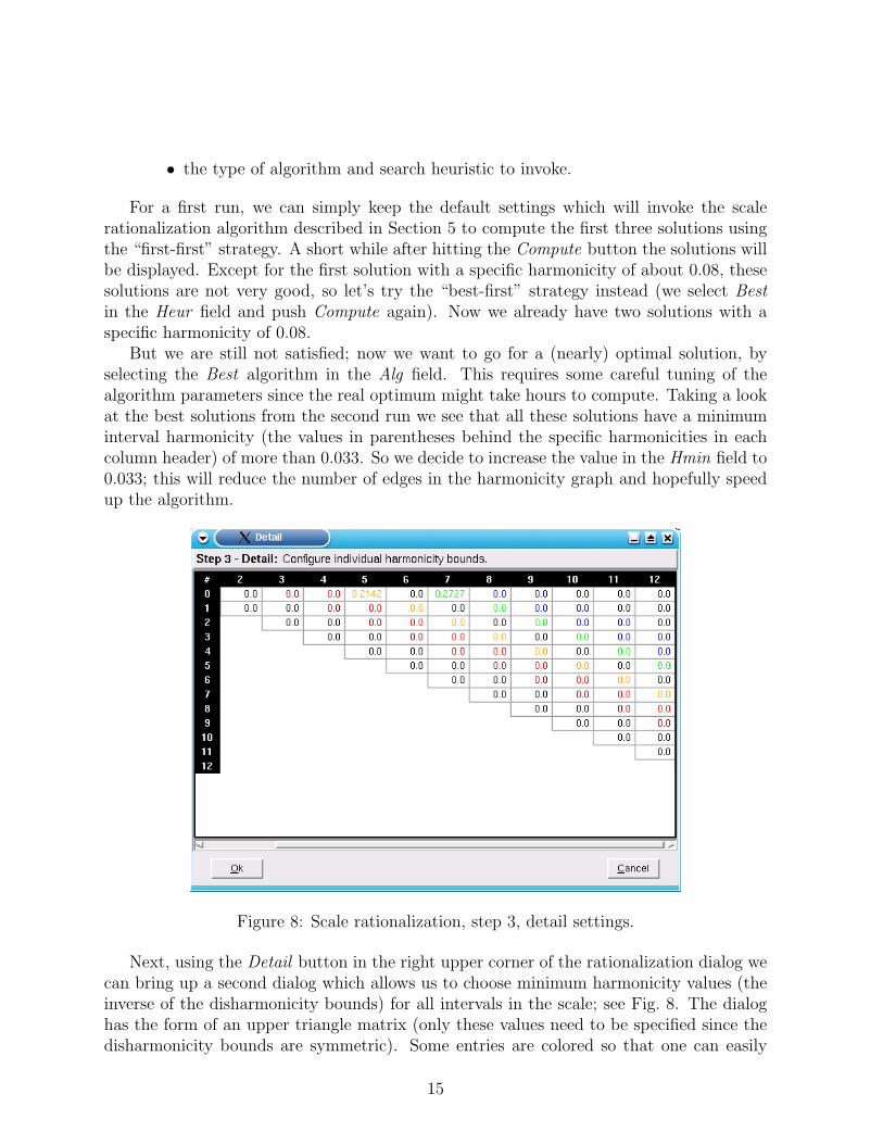
Next, using the Detail button in the right upper corner of the rationalization dialog wecan bring up a second dialog which allows us to choose minimum harmonicity values (theinverse of the disharmonicity bounds) for all intervals in the scale; see Fig. 8. The dialoghas the form of an upper triangle matrix (only these values need to be specified since thedisharmonicity bounds are symmetric). Some entries are colored so that one can easily

15

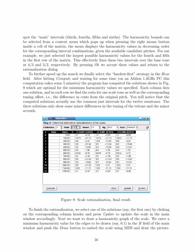
spot the “main” intervals (thirds, fourths, fifths and sixths). The harmonicity bounds canbe selected from a context menu which pops up when pressing the right mouse buttoninside a cell of the matrix; the menu displays the harmonicity values in decreasing orderfor the corresponding interval combinations, given the available candidate pitches. For ourexample, we just selected the largest possible harmonicity values for the fourth and fifthin the first row of the matrix. This effectively fixes these two intervals over the base toneat 4/3 and 3/2, respectively. By pressing Ok we accept these values and return to therationalization dialog.

To further speed up the search we finally select the “hardest-first” strategy in the Heurfield. After hitting Compute and waiting for some time (on an Athlon 1.4GHz PC thiscomputation takes some 5 minutes) the program has computed the solutions shown in Fig.9 which are optimal for the minimum harmonicity values we specified. Each column listsone solution, and in each row we find the ratio for one scale tone as well as the correspondingtuning offset, i.e., the difference in cents from the original pitch. You will notice that thecomputed solutions actually use the common just intervals for the twelve semitones. Thethree solutions only show some minor differences in the tuning of the tritone and the minorseventh.

Figure 9: Scale rationalization, final result.

To finish the rationalization, we select one of the solutions (say, the first one) by clickingon the corresponding column header and press Update to update the scale in the mainwindow accordingly. Next we want to draw a harmonicity graph of the scale. We enter aminimum harmonicity value for the edges to be drawn (say, 0.1) in the H field of the mainwindow and push the Draw button to embed the scale using MDS and draw the picture.

16

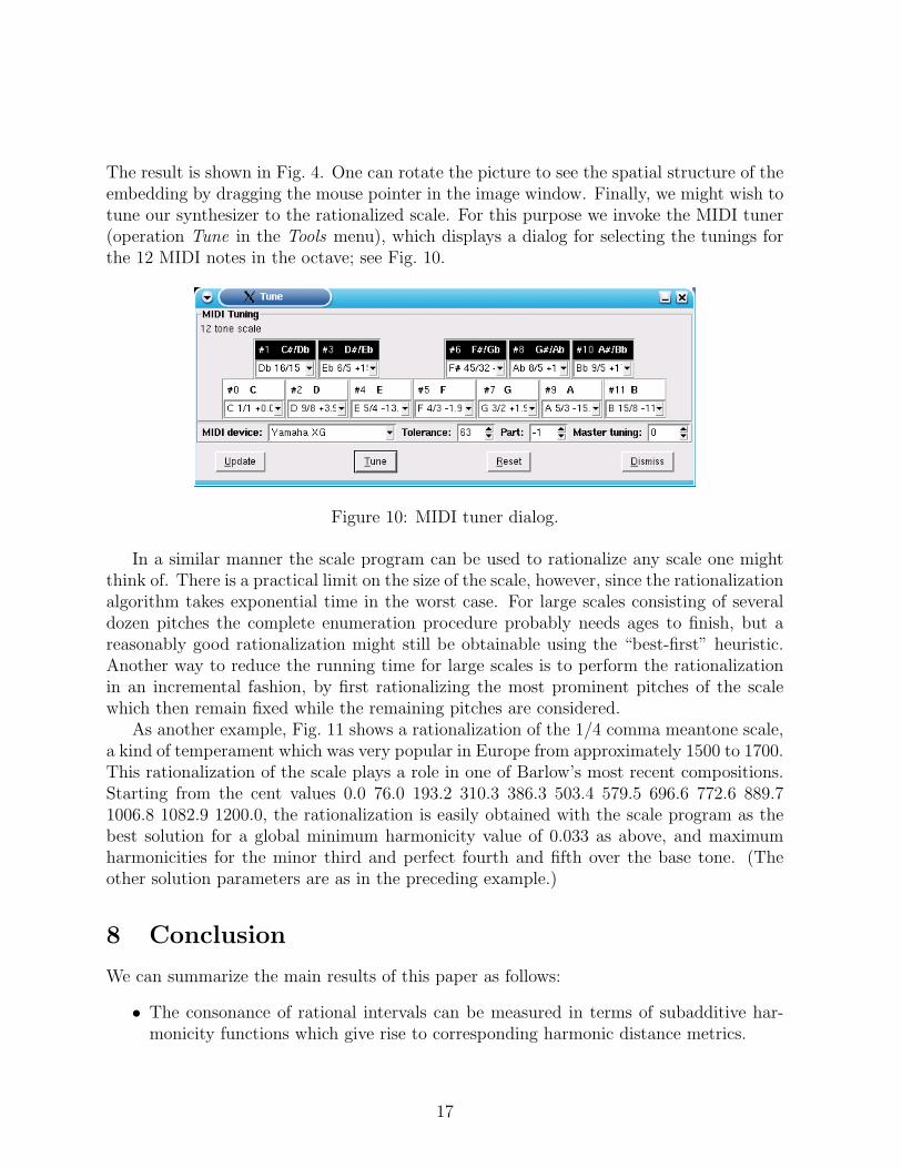
The result is shown in Fig. 4. One can rotate the picture to see the spatial structure of theembedding by dragging the mouse pointer in the image window. Finally, we might wish totune our synthesizer to the rationalized scale. For this purpose we invoke the MIDI tuner(operation Tune in the Tools menu), which displays a dialog for selecting the tunings forthe 12 MIDI notes in the octave; see Fig. 10.

Figure 10: MIDI tuner dialog.

In a similar manner the scale program can be used to rationalize any scale one mightthink of. There is a practical limit on the size of the scale, however, since the rationalizationalgorithm takes exponential time in the worst case. For large scales consisting of severaldozen pitches the complete enumeration procedure probably needs ages to finish, but areasonably good rationalization might still be obtainable using the “best-first” heuristic.Another way to reduce the running time for large scales is to perform the rationalizationin an incremental fashion, by first rationalizing the most prominent pitches of the scalewhich then remain fixed while the remaining pitches are considered.

As another example, Fig. 11 shows a rationalization of the 1/4 comma meantone scale,a kind of temperament which was very popular in Europe from approximately 1500 to 1700.This rationalization of the scale plays a role in one of Barlow’s most recent compositions.Starting from the cent values 0.0 76.0 193.2 310.3 386.3 503.4 579.5 696.6 772.6 889.71006.8 1082.9 1200.0, the rationalization is easily obtained with the scale program as thebest solution for a global minimum harmonicity value of 0.033 as above, and maximumharmonicities for the minor third and perfect fourth and fifth over the base tone. (Theother solution parameters are as in the preceding example.)

8 Conclusion

We can summarize the main results of this paper as follows:

• The consonance of rational intervals can be measured in terms of subadditive har-monicity functions which give rise to corresponding harmonic distance metrics.

17

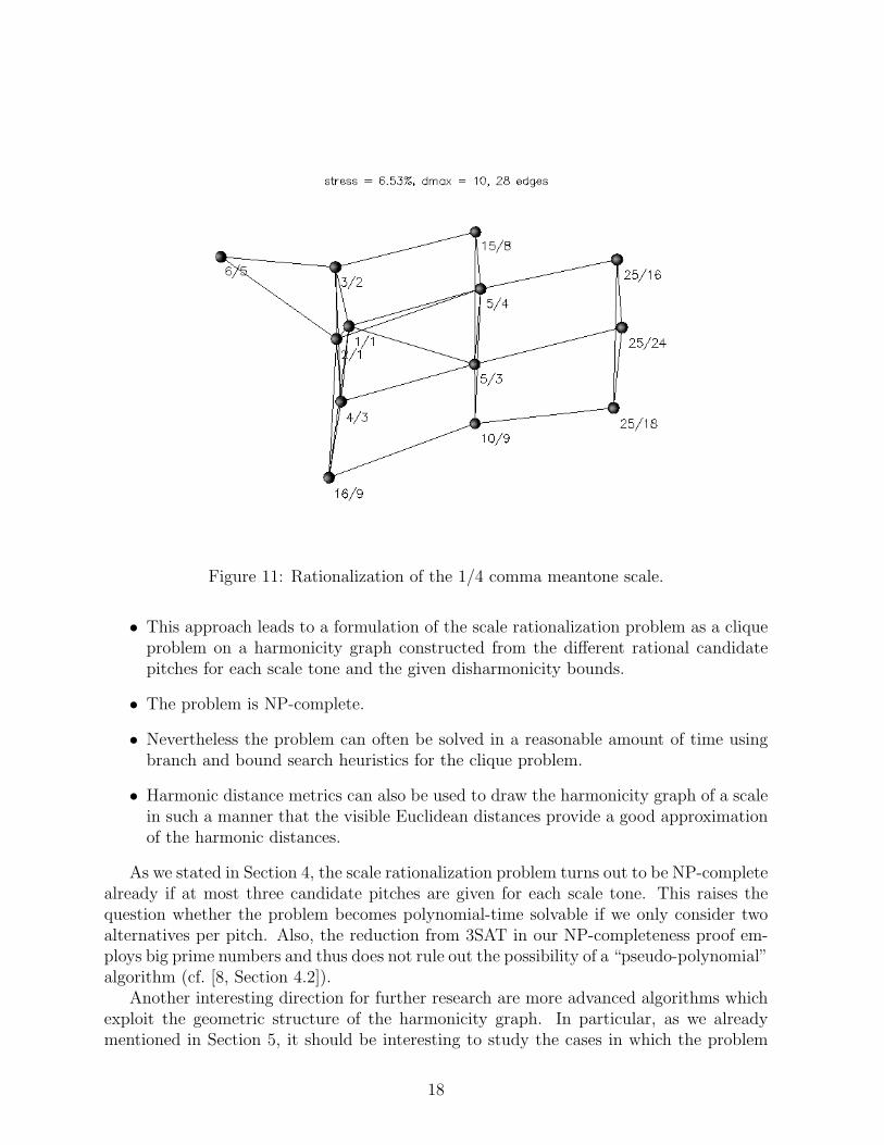
Figure 11: Rationalization of the 1/4 comma meantone scale.

• This approach leads to a formulation of the scale rationalization problem as a cliqueproblem on a harmonicity graph constructed from the different rational candidatepitches for each scale tone and the given disharmonicity bounds.

• The problem is NP-complete.

• Nevertheless the problem can often be solved in a reasonable amount of time usingbranch and bound search heuristics for the clique problem.

• Harmonic distance metrics can also be used to draw the harmonicity graph of a scalein such a manner that the visible Euclidean distances provide a good approximationof the harmonic distances.

As we stated in Section 4, the scale rationalization problem turns out to be NP-completealready if at most three candidate pitches are given for each scale tone. This raises thequestion whether the problem becomes polynomial-time solvable if we only consider twoalternatives per pitch. Also, the reduction from 3SAT in our NP-completeness proof em-ploys big prime numbers and thus does not rule out the possibility of a “pseudo-polynomial”algorithm (cf. [8, Section 4.2]).

Another interesting direction for further research are more advanced algorithms whichexploit the geometric structure of the harmonicity graph. In particular, as we alreadymentioned in Section 5, it should be interesting to study the cases in which the problem

18

can be solved using matching techniques. Unfortunately, it does not seem that thesetechniques will help to solve the optimization version of the problem in which, e.g., thespecific harmonicity is to be maximized.

Yet another topic for future research are other potential applications. For instance, ithas been pointed out by Barlow that scale rationalization techniques can also be used totune instruments in realtime and to perform rhythmic quantization. Our methods shouldbe applicable to these problems as well, provided that the number of pitches or timeintervals to be considered at the same time is not too large.

Acknowledgements

I would like to thank Clarence Barlow for introducing me to the topic of scale rational-ization, for many enlightening discussions, and for commenting on earlier drafts of thispaper.

References

[1] C. Barlow. On the quantification of harmony and metre. In C. Barlow, editor, TheRatio Book, Feedback Papers 43, pages 2–23. Feedback Publishing Company, Cologne,2001.

[2] I. Borg and P. Groenen. Modern Multidimensional Scaling. Springer Series in Statis-tics. Springer, New York, 1997.

[3] R. Carraghan and P. M. Pardalos. An exact algorithm for the maximum clique prob-lem. Operations Research Letters, 9:375–382, 1990.

[4] J. Chalmers. The Divisions of the Tetrachord. Frog Peak Music, 1993.

[5] B. N. Clark, C. J. Colbourn, and D. S. Johnson. Unit disk graphs. Discrete Mathe-matics, 86:165–177, 1990.

[6] P. Erlich. On harmonic entropy. Mills College Tuning Digest, 1997. See http:

//sonic-arts.org/td/entropy.htm.

[7] L. Euler. Tentamen novae theoriae musicae ex certissimis harmoniae principiis dilucideexpositae. St. Petersburg, 1739.

[8] M. R. Garey and D. S. Johnson. Computers and Intractability: A Guide to the Theoryof NP-Completeness. W. H. Freeman and Company, New York, 1979.

[9] H. v. Helmholtz. Die Lehre von den Tonempfindungen als physiologische Grundlagefur die Theorie der Musik. Vieweg, Hildesheim, 6th edition, 1983.

19

[10] J. B. Kruskal. Nonmetric multidimensional scaling: a numerical method. Psychome-trika, 29:115–129, 1964.

[11] J. Tenney. A History of ‘Consonance’ and ‘Dissonance’. Excelsior Music PublishingCompany, New York, 1988.

[12] W. S. Torgerson. Multidimensional scaling: I. Theory and method. Psychometrika,17:401–419, 1952.

20