Metabolomic Data Analysis with MetaboAnalyst

User ID: guest4965371694680211620

April 14, 2009

1 Data Processing and Normalization

1.1 Reading and Processing the Raw Data

MetaboAnalyst accepts a variety of data types generated in metabolomic stud-ies, including compound concentration data, binned NMR/MS spectra data,NMR/MS peak list data, as well as MS spectra (NetCDF, mzXML, mzDATA).Users need to specify the data types when uploading their data in order forMetaboAnalyst to select the correct algorithm to process them.

The R scripts datautils.R and processing.R are required to read in andprocess the uploaded data.

1.1.1 Reading Concentration Data

The concentration data should be uploaded in comma separated values (.csv)format. Samples can be in rows or columns, with class labels immediatelyfollowing the sample IDs.

The uploaded file is in comma separated values (.csv) format. Samples arein rows and features in columns The uploaded data file contains 57 (samples)by 54 (compounds) data matrix.

1.1.2 Data Integrity Check

Before data analysis, a data integrity check is performed to make sure that allthe necessary information has been collected. The class labels must be presentand contain only two classes. If samples are paired, the class label must befrom -n/2 to -1 for one group, and 1 to n/2 for the other group (n is the samplenumber and must be an even number). Class labels with same absolute valueare assumed to be pairs. Compound concentration or peak intensity values mustall be non-negative numbers.

1

1.1.3 Missing value imputations

Too many zeroes or missing values will cause difficulties for downstream analysis.MetaboAnalyst offers several different methods for this purpose. The defaultmethod replaces all the missing and zero values with a small values (the half ofthe minimum positive values in the original data) assuming to be the detectionlimit. The assumption of this approach is that most missing values are causedby low abundance metabolites (i.e.below the detection limit). In addition, sincezero values may cause problem for data normalization (i.e. log), they are alsoreplaced with this small value. User can also specify other methods, such asreplace by mean/median, or use Probabilistic PCA (PPCA), Bayesian PCA(BPCA) method, Singular Value Decomposition (SVD) method to impute themissing values 1. Please choose the one that is the most appropriate for yourdata. Table 1 summarizes the result of the data processing steps.

Missing variables were replaced with a small value: 0.5

1Stacklies W, Redestig H, Scholz M, Walther D, Selbig J. pcaMethods: a bioconductorpackage, providing PCA methods for incomplete data., Bioinformatics 2007 23(9):1164-1167

2

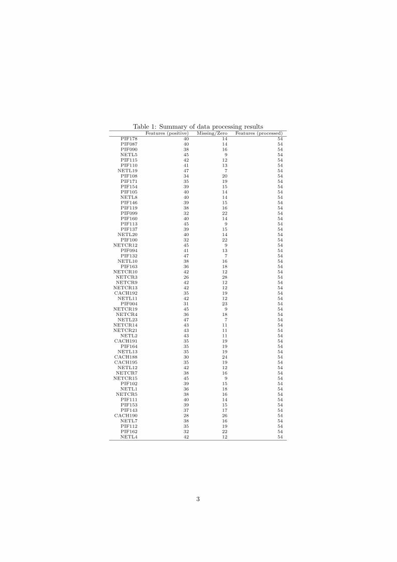
Table 1: Summary of data processing resultsFeatures (positive) Missing/Zero Features (processed)

PIF178 40 14 54PIF087 40 14 54PIF090 38 16 54NETL5 45 9 54PIF115 42 12 54PIF110 41 13 54

NETL19 47 7 54PIF108 34 20 54PIF171 35 19 54PIF154 39 15 54PIF105 40 14 54NETL8 40 14 54PIF146 39 15 54PIF119 38 16 54PIF099 32 22 54PIF160 40 14 54PIF113 45 9 54PIF137 39 15 54

NETL20 40 14 54PIF100 32 22 54

NETCR12 45 9 54PIF094 41 13 54PIF132 47 7 54

NETL10 38 16 54PIF163 36 18 54

NETCR10 42 12 54NETCR3 26 28 54NETCR9 42 12 54

NETCR13 42 12 54CACH192 35 19 54NETL11 42 12 54PIF004 31 23 54

NETCR19 45 9 54NETCR4 36 18 54NETL23 47 7 54

NETCR14 43 11 54NETCR21 43 11 54

NETL2 43 11 54CACH191 35 19 54

PIF164 35 19 54NETL13 35 19 54

CACH188 30 24 54CACH195 35 19 54NETL12 42 12 54NETCR7 38 16 54

NETCR15 45 9 54PIF102 39 15 54NETL1 36 18 54

NETCR5 38 16 54PIF111 40 14 54PIF153 39 15 54PIF143 37 17 54

CACH190 28 26 54NETL7 38 16 54PIF112 35 19 54PIF162 32 22 54NETL4 42 12 54

3

1.2 Data Normalization

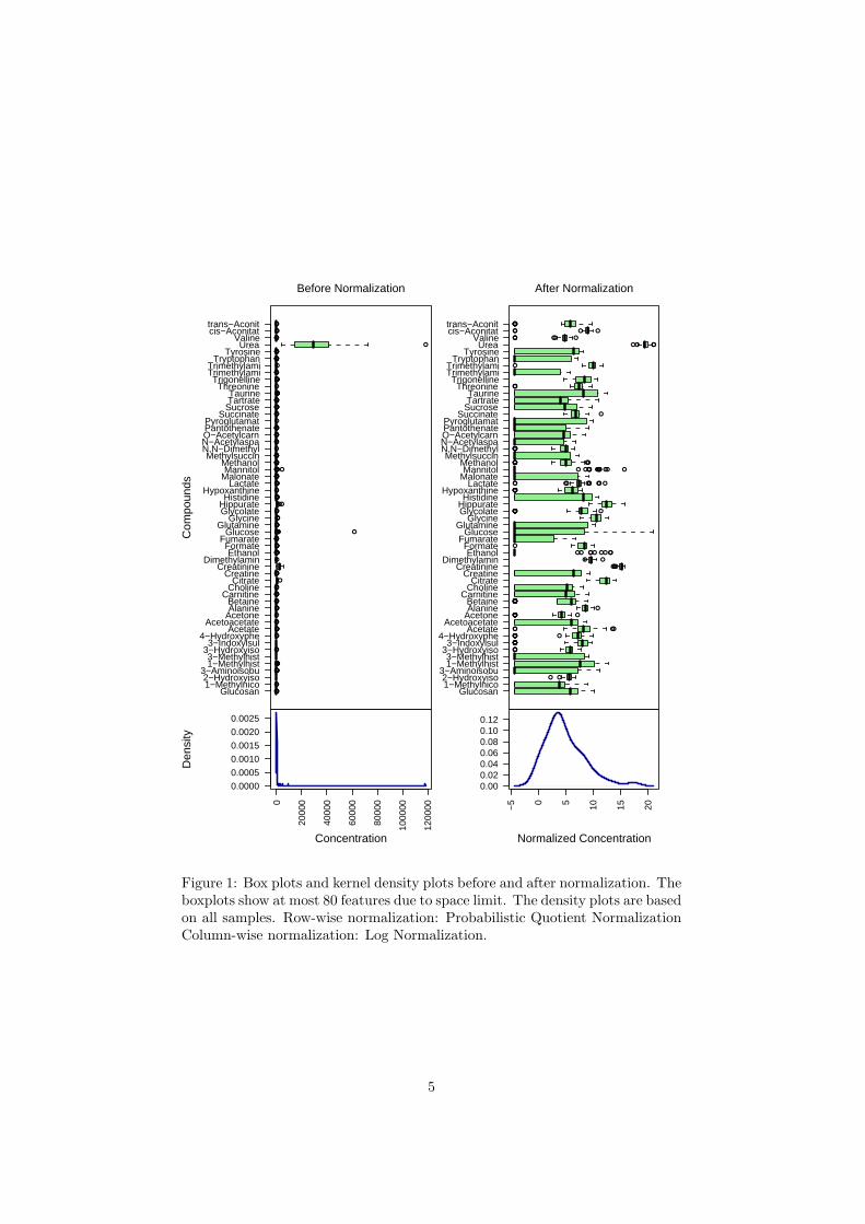
The data is stored as a table with one sample per row and one variable (bin/peak/metabolite) per column. There are two types of normalization. Row-wise normalization aims to bring each sample (row) comparable to each other(i.e. urine samples with different dilution effects). Column-wise normalizationaims to make each variable (column) comparable to each other within the samesample. The procedure is useful when variables are of very different orders ofmagnitude.

The normalization consists of the following options:

1. Row-wise normalization:

� Normalization by the sum

� Normalization by a reference sample (probabilistic quotient normal-ization) 2

� Normalization by a reference feature (i.e. creatinine, internal control)

� Sample specific normalization (i.e. normalize by dry weight, volume)

2. Column-wise normalization :

� Log transformation (log 2)

� Unit scaling (mean-centered and divided by standard deviation ofeach variable)

� Pareto scaling (mean-centered and divided by the square root of stan-dard deviation of each variable)

� Range scaling (mean-centered and divided by the value range of eachvariable)

The R script normalization.R is required. Figure 1 shows the effects beforeand after normalization.

2Dieterle F, Ross A, Schlotterbeck G, Senn H. Probabilistic quotient normalization asrobust method to account for dilution of complex biological mixtures. Application in 1H NMRmetabonomics, 2006, Anal Chem 78 (13);4281 - 4290

4

●●●●●

●●

●●●●●●

●●●●●●●

●●

●●

●●●●

●●●

●

●●●

●●●●

●●●●●●●●

●●●

●

●●●●●

●

●●●●●●●●●

●●●●●

●●●●●●●

●●●● ●●●●●

●●●●●

●●●

●●

●●

●●●●●●

●●

●●●●●

●●●●●●●●●

●●●●● ●●●●●●●●●

●●●●●●●●

●●●●●●●

●

●●●

●●●●●

●●●●●●●●●

●

●●●●●

●●●●●●●●●

●●●●●●●●

●●●●●●●

●

●●●●●●●●

●●●●

●

●●●●●●●●

●●●●●●

●

●●●●

●●

●●

Glucosan1−Methylnico2−Hydroxyiso

3−Aminoisobu1−Methylhist3−Methylhist

3−Hydroxyiso3−Indoxylsul

4−HydroxypheAcetate

AcetoacetateAcetoneAlanineBetaine

CarnitineCholineCitrate

CreatineCreatinine

DimethylaminEthanol

FormateFumarate

GlucoseGlutamine

GlycineGlycolateHippurateHistidine

HypoxanthineLactate

MalonateMannitol

MethanolMethylsuccin

N,N−DimethylN−AcetylaspaO−AcetylcarnPantothenatePyroglutamat

SuccinateSucroseTartrateTaurine

ThreonineTrigonelline

TrimethylamiTrimethylami

TryptophanTyrosine

UreaValine

cis−Aconitattrans−Aconit

Com

poun

ds

Before Normalization0

2000

0

4000

0

6000

0

8000

0

1000

00

1200

00

0.0000

0.0005

0.0010

0.0015

0.0020

0.0025

Den

sity

Concentration

● ●

●●●●

●●●●●●●●●●

●●●●●●●●●

●● ●●

●●●●●●●●●●●

●

●●●●●●●●●●●●●●

●●●●

●●

● ●●● ●●●● ●

●

●●●●●●●●●● ●

●●●●●●●●●●

● ● ●●●●●● ●●

●●●● ● ●●●● ●●●● ●

●●●●●●● ●●

●●●●●●●●●

●

●●●●

●

● ●● ●

●●● ●● ●

●●●●

●●●●●●●●●●●

Glucosan1−Methylnico2−Hydroxyiso

3−Aminoisobu1−Methylhist3−Methylhist

3−Hydroxyiso3−Indoxylsul

4−HydroxypheAcetate

AcetoacetateAcetoneAlanineBetaine

CarnitineCholineCitrate

CreatineCreatinine

DimethylaminEthanol

FormateFumarate

GlucoseGlutamine

GlycineGlycolateHippurateHistidine

HypoxanthineLactate

MalonateMannitol

MethanolMethylsuccin

N,N−DimethylN−AcetylaspaO−AcetylcarnPantothenatePyroglutamat

SuccinateSucroseTartrateTaurine

ThreonineTrigonelline

TrimethylamiTrimethylami

TryptophanTyrosine

UreaValine

cis−Aconitattrans−Aconit

After Normalization

−5 0 5 10 15 20

0.000.020.040.060.080.100.12

Normalized Concentration

Figure 1: Box plots and kernel density plots before and after normalization. Theboxplots show at most 80 features due to space limit. The density plots are basedon all samples. Row-wise normalization: Probabilistic Quotient NormalizationColumn-wise normalization: Log Normalization.

5

2 Statistical and Machine Learning Data Anal-ysis

MetaboAnalyst offers a variety of methods commonly used in metabolomic dataanalyses. They include:

1. Univariate analysis methods:

� Fold Change Analysis

� T-tests

� Volcano Plot

2. Dimensional Reduction methods:

� Principal Component Analysis (PCA)

� Partial Least Squares - Discriminant Analysis (PLS-DA)

3. Robust Feature Selection Methods in microarray studies

� Significance Analysis of Microarray (SAM)

� Empirical Bayesian Analysis of Microarray (EBAM)

4. Clustering Analysis

� Hierarchical Clustering

– Dendrogram– Heatmap

� Partitional Clustering

– K-means Clustering– Self-Organizing Map (SOM)

5. Supervised Classification and Feature Selection methods

� Random Forest

� Support Vector Machine (SVM)

6

2.1 Univariate Analysis

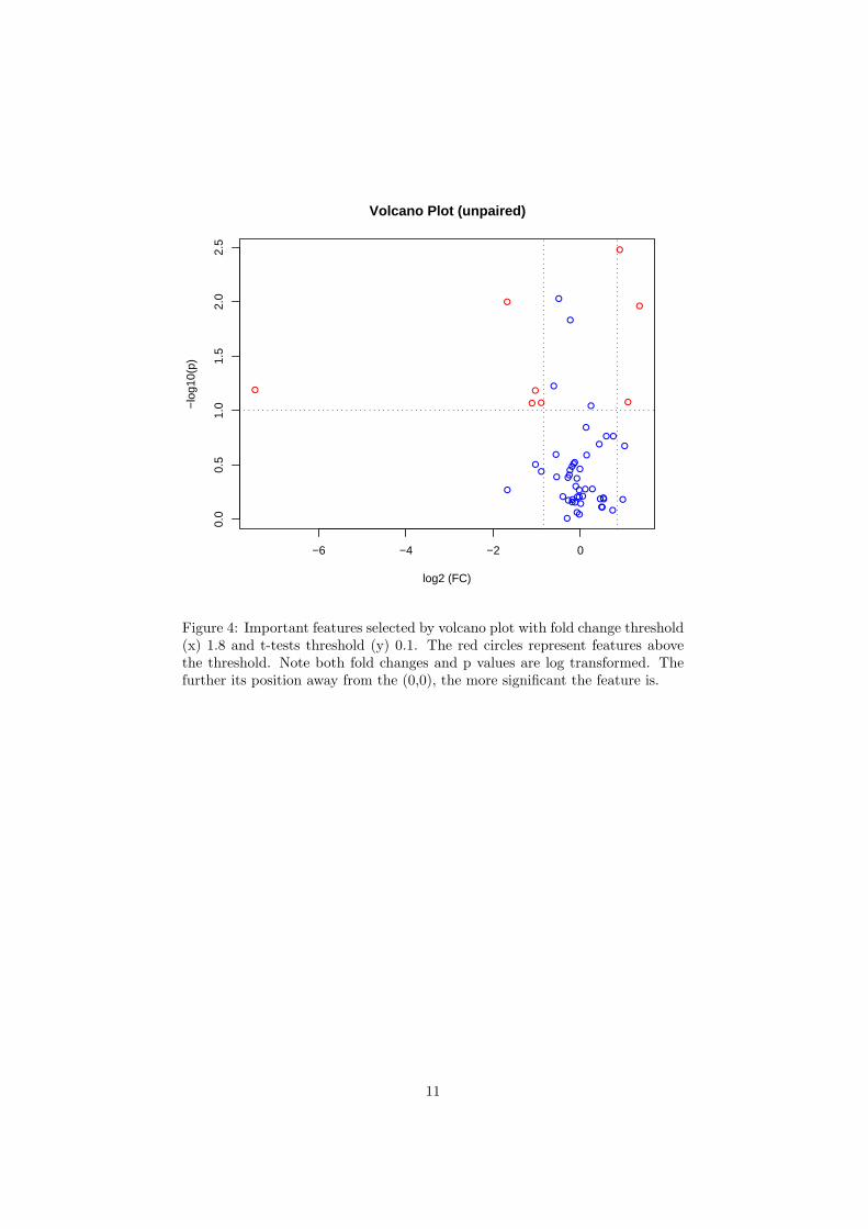
There are three methods available for univariate analyses, including Fold Change(FC) analysis, t-tests, and volcano plot which is a combination of the first twomethods. All three these methods support both unpaired and paired analy-ses. They provide a preliminary overview about features that are potentiallysignificant in discriminating the two groups under study.

For paired fold change analysis, the algorithm first counts the total numberof pairs with fold changes that are consistently above/below the specified FCthreshold for each variable. A variable will be reported as significant if thisnumber is above a given count threshold (default > 75% of pairs/variable)

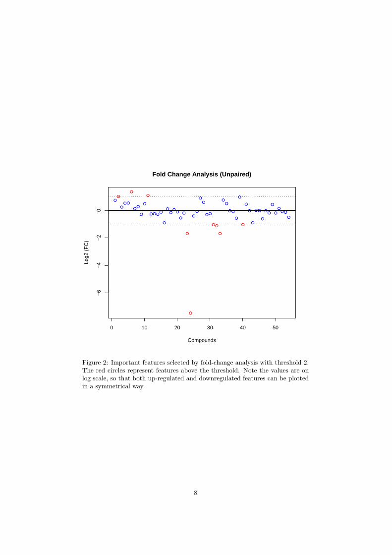
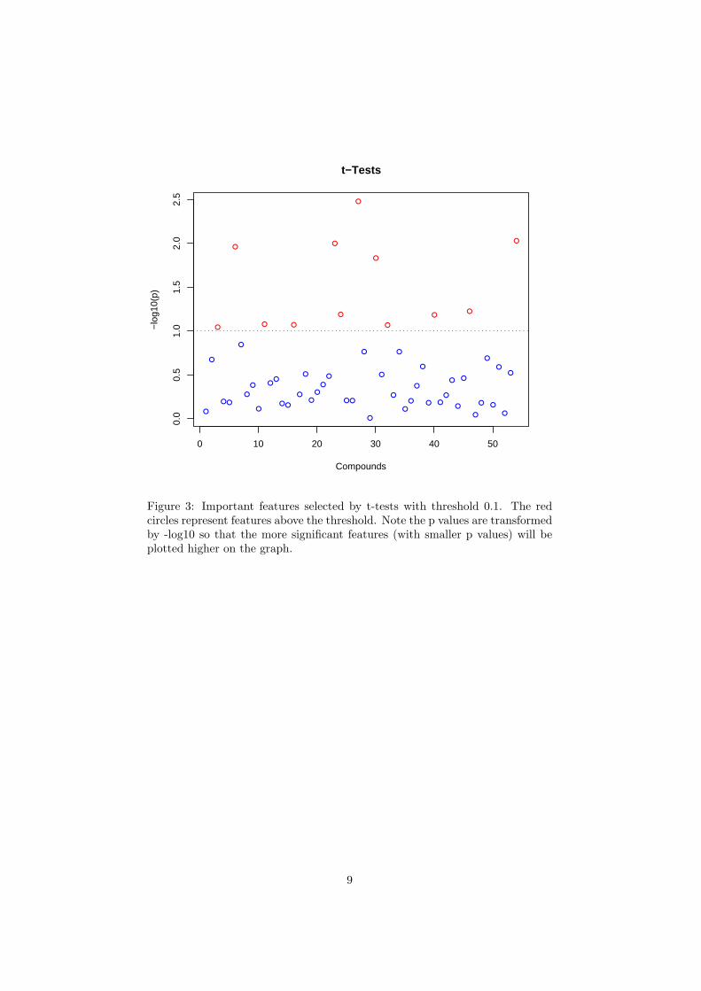
The R script univartests.R is required. Figure 2 shows the importantfeatures identified by fold change analysis. Table 2 shows the details of thesefeatures; Figure 3 shows the important features identified by t-tests. Table3 shows the details of these features; Figure 4 shows the important featuresidentified by volcano plot. Table 4 shows the details of these features.

Please note, the purpose of fold change is to compare absolute value changesbetween two group means. Therefore, the data before column normlaization willbe used instead. Also note, the result is plotted in log2 scale, so that same foldchange (up/down-regulated) will have the same distance to the zero baseline.

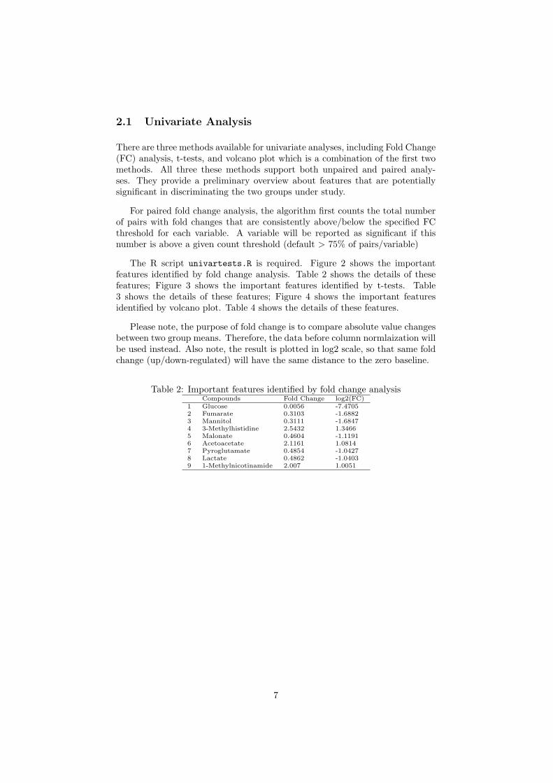
Table 2: Important features identified by fold change analysisCompounds Fold Change log2(FC)

1 Glucose 0.0056 -7.47052 Fumarate 0.3103 -1.68823 Mannitol 0.3111 -1.68474 3-Methylhistidine 2.5432 1.34665 Malonate 0.4604 -1.11916 Acetoacetate 2.1161 1.08147 Pyroglutamate 0.4854 -1.04278 Lactate 0.4862 -1.04039 1-Methylnicotinamide 2.007 1.0051

7

●●

●● ●

●

●●

●

●

●

● ● ●●

●

●●

●●

●

●

●

●

●

●

●

●

● ●

● ●

●

●●

● ●

●

●

●

●

●

●

● ●

●

●●

●

●

●● ●

●

0 10 20 30 40 50

−6

−4

−2

0

Fold Change Analysis (Unpaired)

Compounds

Log2

(F

C)

Figure 2: Important features selected by fold-change analysis with threshold 2.The red circles represent features above the threshold. Note the values are onlog scale, so that both up-regulated and downregulated features can be plottedin a symmetrical way

8

●

●

●

● ●

●

●

●

●

●

●

●●

● ●

●

●

●

●

●

●

●

●

●

● ●

●

●

●

●

●

●

●

●

●

●

●

●

●

●

●

●

●

●

●

●

●

●

●

●

●

●

●

●

0 10 20 30 40 50

0.0

0.5

1.0

1.5

2.0

2.5

t−Tests

Compounds

−lo

g10(

p)

Figure 3: Important features selected by t-tests with threshold 0.1. The redcircles represent features above the threshold. Note the p values are transformedby -log10 so that the more significant features (with smaller p values) will beplotted higher on the graph.

9

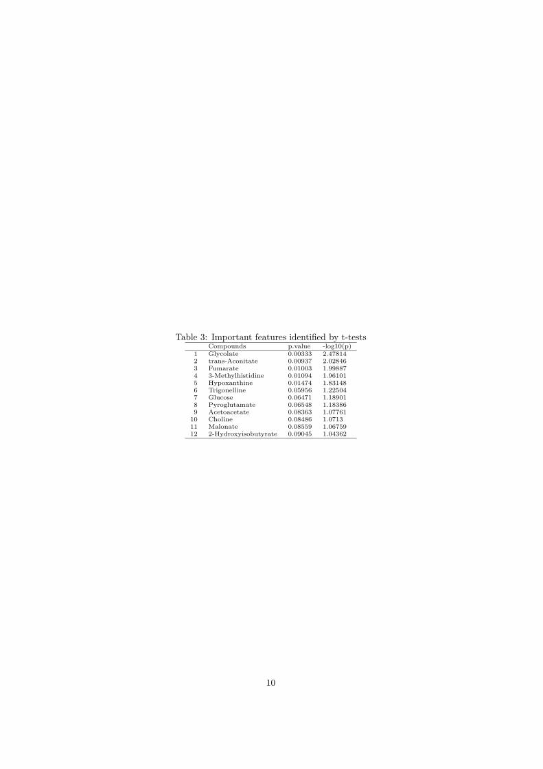
Table 3: Important features identified by t-testsCompounds p.value -log10(p)

1 Glycolate 0.00333 2.478142 trans-Aconitate 0.00937 2.028463 Fumarate 0.01003 1.998874 3-Methylhistidine 0.01094 1.961015 Hypoxanthine 0.01474 1.831486 Trigonelline 0.05956 1.225047 Glucose 0.06471 1.189018 Pyroglutamate 0.06548 1.183869 Acetoacetate 0.08363 1.07761

10 Choline 0.08486 1.071311 Malonate 0.08559 1.0675912 2-Hydroxyisobutyrate 0.09045 1.04362

10

●

●

●

●●

●

●

●

●

●

●

●●

●●

●

●

●

●

●

●

●

●

●

● ●

●

●

●

●

●

●

●

●

●

●

●

●

●

●

●

●

●

●

●

●

●

●

●

●

●

●

●

●

−6 −4 −2 0

0.0

0.5

1.0

1.5

2.0

2.5

Volcano Plot (unpaired)

log2 (FC)

−lo

g10(

p)

Figure 4: Important features selected by volcano plot with fold change threshold(x) 1.8 and t-tests threshold (y) 0.1. The red circles represent features abovethe threshold. Note both fold changes and p values are log transformed. Thefurther its position away from the (0,0), the more significant the feature is.

11

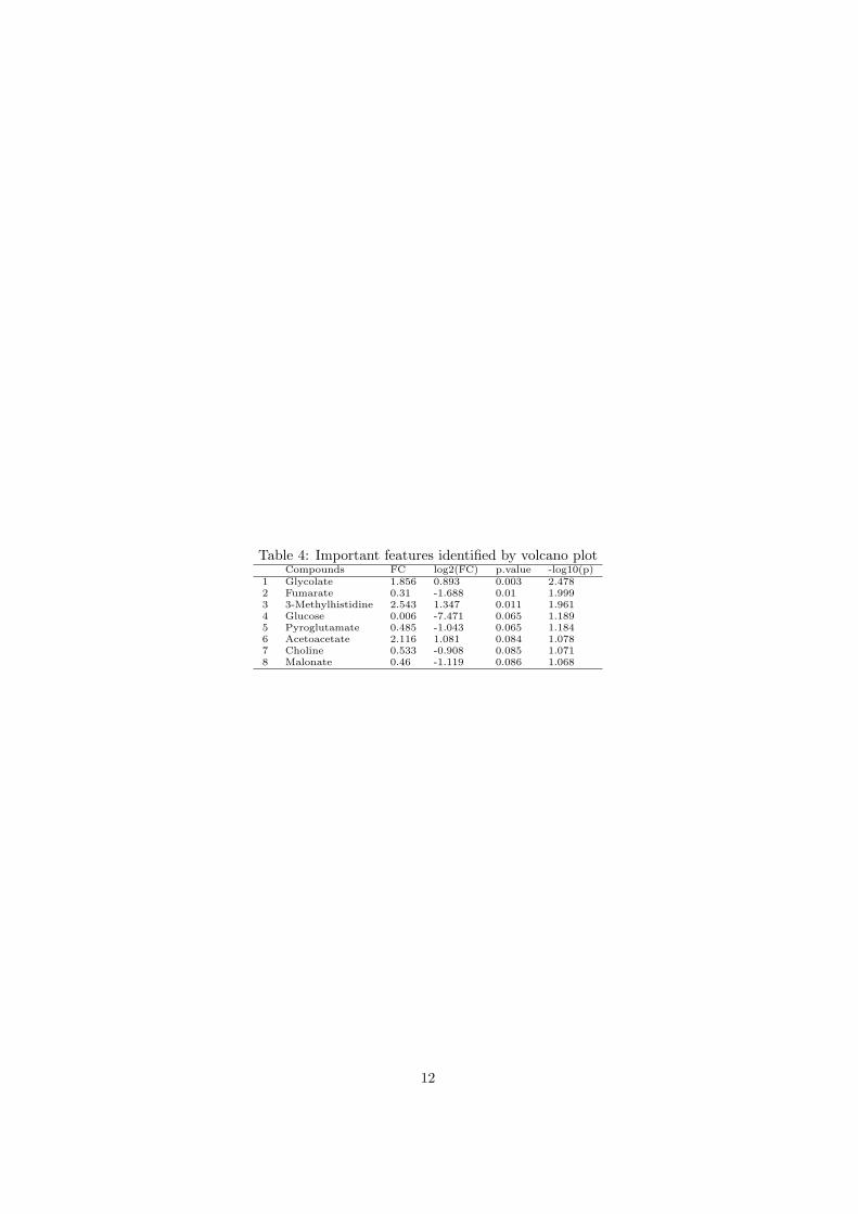
Table 4: Important features identified by volcano plotCompounds FC log2(FC) p.value -log10(p)

1 Glycolate 1.856 0.893 0.003 2.4782 Fumarate 0.31 -1.688 0.01 1.9993 3-Methylhistidine 2.543 1.347 0.011 1.9614 Glucose 0.006 -7.471 0.065 1.1895 Pyroglutamate 0.485 -1.043 0.065 1.1846 Acetoacetate 2.116 1.081 0.084 1.0787 Choline 0.533 -0.908 0.085 1.0718 Malonate 0.46 -1.119 0.086 1.068

12

2.2 Partial Least Squares - Discriminant Analysis (PLS-DA)

PLS is a supervised method that uses multivariate regression techniques toextract via linear combination of original variables (X) the information thatcan predict the class membership (Y). The PLS regression is performed usingthe plsr function provided by R pls package3. The classification and cross-validation are performed using the corresponding wrapper function offered bythe caret package4.

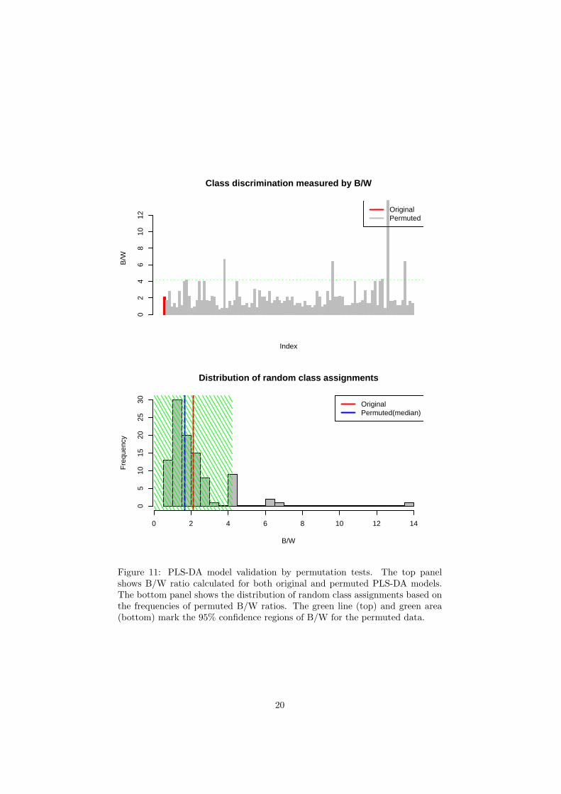
To assess the significance of class discrimination, a permutation test wasperformed. In each permutation, a PLS-DA model was built between the data(X) and the permuted class labels (Y) using the optimal number of compo-nents determined by cross validation for the model based on the original classassignment. The ratio of the between sum of the squares and the within sumof squares (B/W-ratio) for the class assignment prediction of each model wascalculated. If the B/W ratio of the original class assignment is a part of thedistribution based on the permuted class assignments The contrast between thetwo class assignment cannot be considered significant from a statistical point ofview.

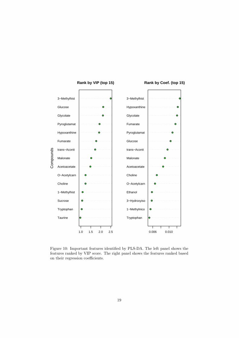
There are two variable importance measures in PLS-DA. The first, VariableImportance in Projection (VIP) is a weighted sum of squares of the PLS loadingstaking into account the amount of explained Y-variation in each dimension. Theother importance measure is based on the weighted sum of PLS-regression Theweights are a function of the reduction of the sums of squares across the numberof PLS components. coefficients5.

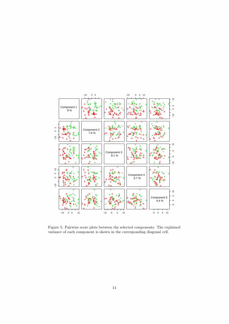
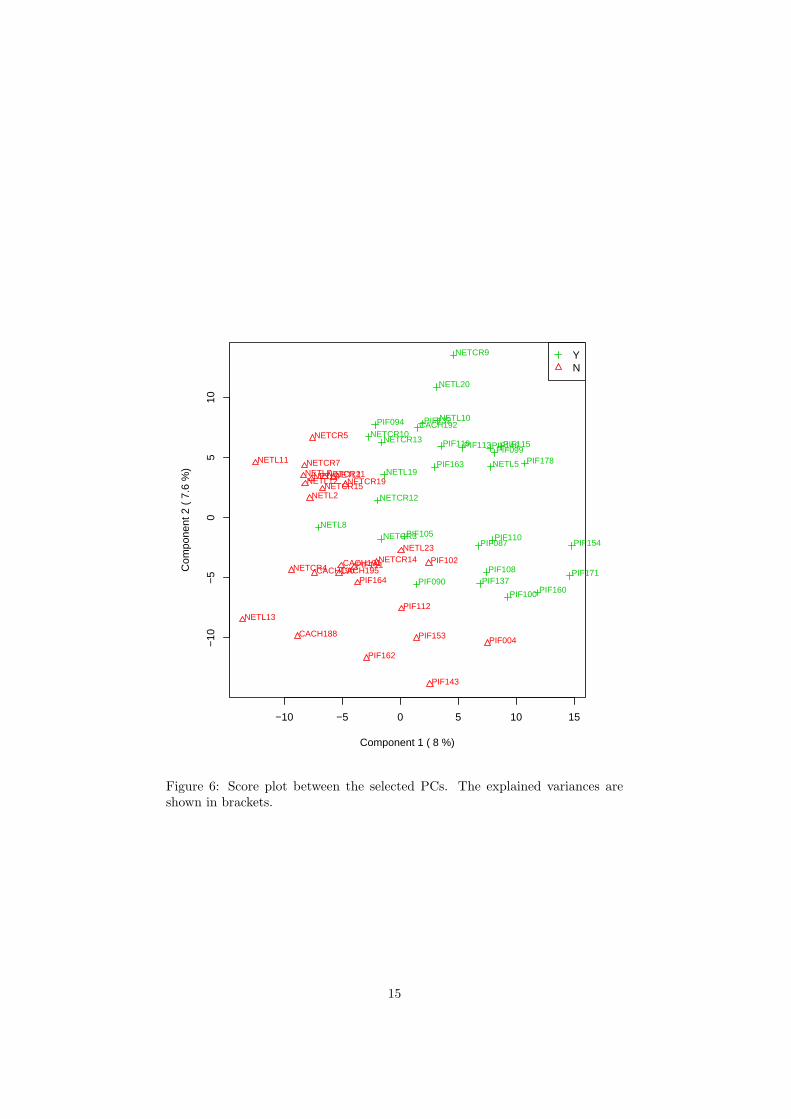
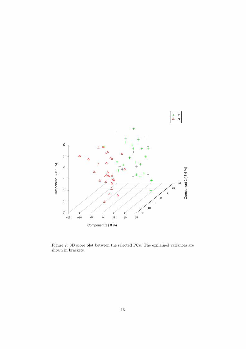
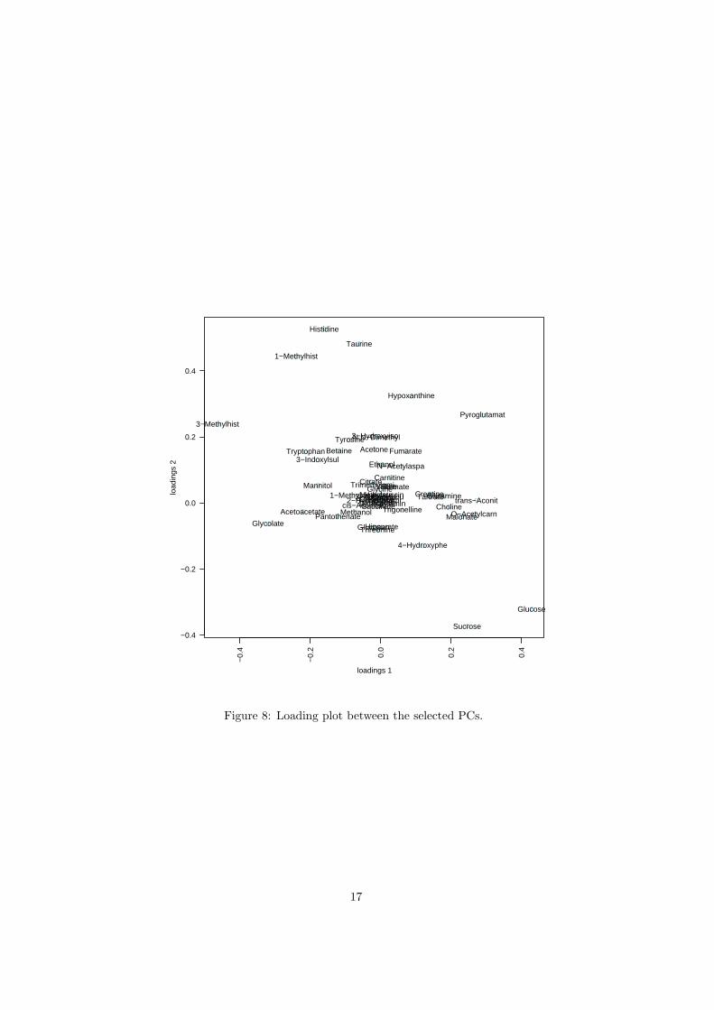
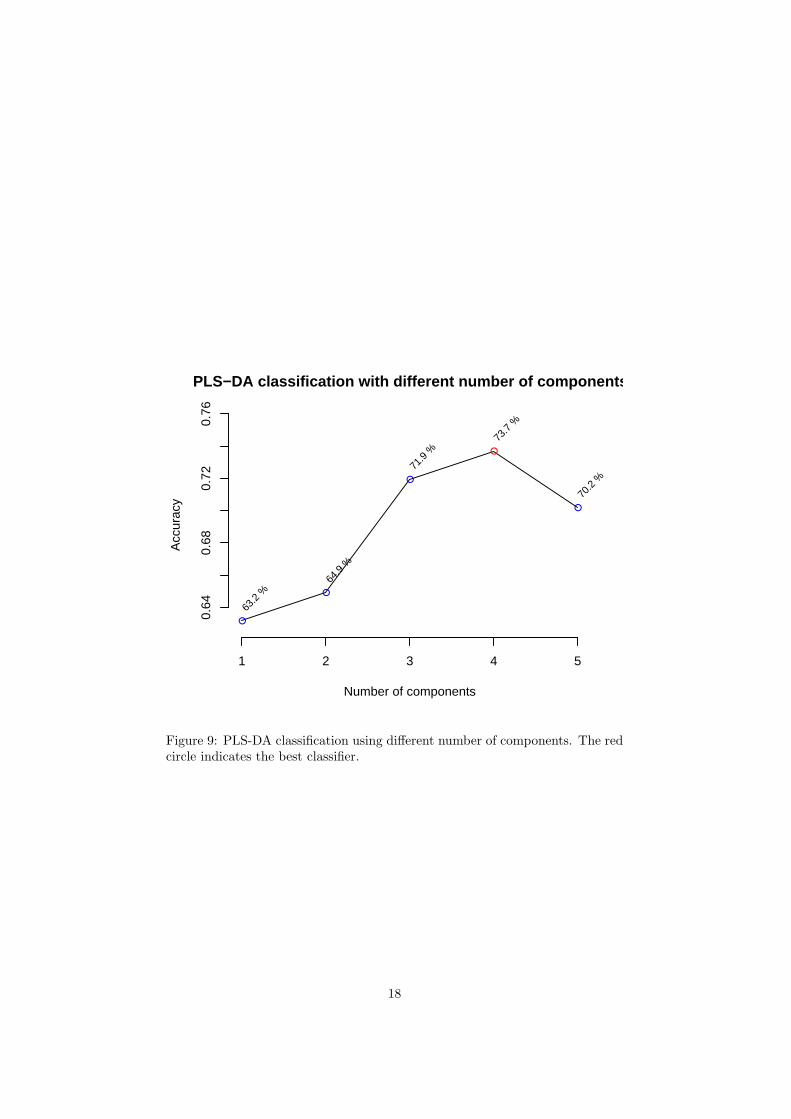
The R script chemometrics.R is required. Figure 5 shows the overview ofscore plots; Figure 6 shows the 2-D score plot between selected components;Figure 7 shows the 3-D score plot between selected components; Figure 8 showsthe loading plot between the selected components; Figure 9 shows the classifi-cation performance with different number of components. Figure 10 shows theimportant features identified by PLS-DA. Figure 11 shows the permutation testresults for model validation.

3Ron Wehrens and Bjorn-Helge Mevik.pls: Partial Least Squares Regression (PLSR) andPrincipal Component Regression (PCR), 2007, R package version 2.1-0

4Max Kuhn. Contributions from Jed Wing and Steve Weston and Andre Williams.caret:Classification and Regression Training, 2008, R package version 3.45

5Bijlsma et al.Large-Scale Human Metabolomics Studies: A Strategy for Data (Pre-) Pro-cessing and Validation, Anal Chem. 2006, 78 567 - 574

13

Component 1 8 %

−10 0 5 −10 0 5 10

−10

05

15

−10

05

Component 2 7.6 %

Component 3 8.1 %

−15

−5

515

−10

05

10

Component 4 5.7 %

−10 0 5 15 −15 −5 5 15 −5 0 5 10

−5

05

10

Component 5 4.4 %

Figure 5: Pairwise score plots between the selected components. The explainedvariance of each component is shown in the corresponding diagonal cell.

14

−10 −5 0 5 10 15

−10

−5

05

10

Component 1 ( 8 %)

Com

pone

nt 2

( 7

.6 %

)

PIF178

PIF087

PIF090

NETL5

PIF115

PIF110

NETL19

PIF108 PIF171

PIF154PIF105

NETL8

PIF146PIF119PIF099

PIF160

PIF113

PIF137

NETL20

PIF100

NETCR12

PIF094 PIF132NETL10

PIF163

NETCR10

NETCR3

NETCR9

NETCR13

CACH192

NETL11

PIF004

NETCR19

NETCR4

NETL23NETCR14

NETCR21

NETL2

CACH191

PIF164

NETL13

CACH188

CACH195

NETL12

NETCR7

NETCR15

PIF102

NETL1

NETCR5

PIF111

PIF153

PIF143

CACH190

NETL7

PIF112

PIF162

NETL4

YN

Figure 6: Score plot between the selected PCs. The explained variances areshown in brackets.

15

−15 −10 −5 0 5 10 15

−15

−10

−5

0 5

10

15

−15

−10

−5

0

5

10

15

Component 1 ( 8 %)

Com

pone

nt 2

( 7

.6 %

)

Com

pone

nt 3

( 8

.1 %

)

YN

Figure 7: 3D score plot between the selected PCs. The explained variances areshown in brackets.

16

●

●●

●

●

●

●

●

●

●

●

●

●

●

●

●

●

●●

●

●

●

●

●

●

●

●●

●

●

●

●

●

●

●

●

●

●●

●

●

●

●

●

●

●

●

●

●

●

●

●

●●

−0.

4

−0.

2

0.0

0.2

0.4

−0.4

−0.2

0.0

0.2

0.4

loadings 1

load

ings

2

Glucosan

1−Methylnico2−Hydroxyiso3−Aminoisobu

1−Methylhist

3−Methylhist

3−Hydroxyiso

3−Indoxylsul

4−Hydroxyphe

AcetateAcetoacetate

Acetone

Alanine

Betaine

Carnitine

Choline

Citrate

CreatineCreatinineDimethylamin

Ethanol

Formate

Fumarate

Glucose

GlutamineGlycine

Glycolate Hippurate

Histidine

Hypoxanthine

Lactate

Malonate

Mannitol

Methanol

Methylsuccin

N,N−Dimethyl

N−Acetylaspa

O−AcetylcarnPantothenate

Pyroglutamat

Succinate

Sucrose

Tartrate

Taurine

Threonine

Trigonelline

Trimethylami

Trimethylami

Tryptophan

Tyrosine

Urea

Valine

cis−Aconitattrans−Aconit

Figure 8: Loading plot between the selected PCs.

17

PLS−DA classification with different number of components

Number of components

Acc

urac

y

63.2

%64

.9 %

71.9

%73

.7 %

70.2

%

●

●

●

●

●

0.64

0.68

0.72

0.76

1 2 3 4 5

Figure 9: PLS-DA classification using different number of components. The redcircle indicates the best classifier.

18

Taurine

Tryptophan

Sucrose

1−Methylhist

Choline

O−Acetylcarn

Acetoacetate

Malonate

trans−Aconit

Fumarate

Hypoxanthine

Pyroglutamat

Glycolate

Glucose

3−Methylhist

●

●

●

●

●

●

●

●

●

●

●

●

●

●

●

1.0 1.5 2.0 2.5

Rank by VIP (top 15)

Com

poun

ds

Tryptophan

1−Methylnico

3−Hydroxyiso

Ethanol

O−Acetylcarn

Choline

Acetoacetate

Malonate

trans−Aconit

Glucose

Pyroglutamat

Fumarate

Glycolate

Hypoxanthine

3−Methylhist

●

●

●

●

●

●

●

●

●

●

●

●

●

●

●

0.006 0.010

Rank by Coef. (top 15)

Figure 10: Important features identified by PLS-DA. The left panel shows thefeatures ranked by VIP score. The right panel shows the features ranked basedon their regression coefficients.

19

Class discrimination measured by B/W

Index

B/W

02

46

810

12

OriginalPermuted

Distribution of random class assignments

B/W

Fre

quen

cy

0 2 4 6 8 10 12 14

05

1015

2025

30 OriginalPermuted(median)

Figure 11: PLS-DA model validation by permutation tests. The top panelshows B/W ratio calculated for both original and permuted PLS-DA models.The bottom panel shows the distribution of random class assignments based onthe frequencies of permuted B/W ratios. The green line (top) and green area(bottom) mark the 95% confidence regions of B/W for the permuted data.

20

2.3 Significance Analysis of Microarray (SAM)

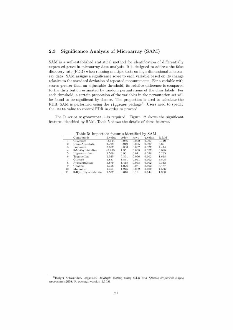
SAM is a well-established statistical method for identification of differentiallyexpressed genes in microarray data analysis. It is designed to address the falsediscovery rate (FDR) when running multiple tests on high-dimensional microar-ray data. SAM assigns a significance score to each variable based on its changerelative to the standard deviation of repeated measurements. For a variable withscores greater than an adjustable threshold, its relative difference is comparedto the distribution estimated by random permutations of the class labels. Foreach threshold, a certain proportion of the variables in the permutation set willbe found to be significant by chance. The proportion is used to calculate theFDR. SAM is performed using the siggenes package6. Users need to specifythe Delta value to control FDR in order to proceed.

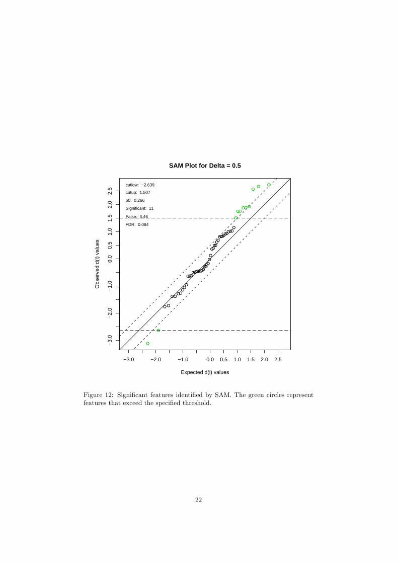
The R script sigfeatures.R is required. Figure 12 shows the significantfeatures identified by SAM. Table 5 shows the details of these features.

Table 5: Important features identified by SAMCompounds d.value stdev rawp q.value R.fold

1 Glycolate -3.114 0.986 0.002 0.027 0.1192 trans-Aconitate 2.729 0.919 0.005 0.027 5.693 Fumarate 2.667 0.803 0.007 0.027 4.4144 3-Methylhistidine -2.639 1.35 0.008 0.027 0.0855 Hypoxanthine 2.569 0.93 0.01 0.028 5.2356 Trigonelline 1.925 0.361 0.056 0.102 1.6187 Glucose 1.887 1.541 0.061 0.102 7.5058 Pyroglutamate 1.879 1.418 0.063 0.102 6.3439 Choline 1.756 1.026 0.081 0.102 3.487

10 Malonate 1.751 1.246 0.082 0.102 4.53611 3-Hydroxyisovalerate 1.507 0.618 0.13 0.144 1.908

6Holger Schwender. siggenes: Multiple testing using SAM and Efron’s empirical Bayesapproaches,2008, R package version 1.16.0

21

● ●

●●●●

●●

●

●●●●●●●●●●●●

●●●●

●

●

●●●●

●●●●●●

●●●●●●

−3.0 −2.0 −1.0 0.0 0.5 1.0 1.5 2.0 2.5

−3.

0−

2.0

−1.

00.

00.

51.

01.

52.

02.

5

SAM Plot for Delta = 0.5

Expected d(i) values

Obs

erve

d d(

i) va

lues

●

●●●● ●

●●

●

●

●

cutlow: −2.639

cutup: 1.507

p0: 0.266

Significant: 11

False: 3.46

FDR: 0.084

Figure 12: Significant features identified by SAM. The green circles representfeatures that exceed the specified threshold.

22

3 Data Annotation

Please be advised that MetaboAnalyst also supports metabolomic data annota-tion. For NMR, MS, or GC-MS peak list data, users can perform peak identi-fication by searching the corresponding libraries. For compound concentrationdata, users can perform pathway mapping. These tasks require a lot of manualefforts and are not performed by default.

——————————–

The report was generated on Tue Apr 14 19:04:35 2009 with R version2.8.1 (2008-12-22) on a i386-redhat-linux-gnu platform. Thank you for usingMetaboAnalyst! For suggestions and feedback please contact Jeff Xia (jian-guox@ualberta.ca).

23