Meta Optimization and its Application to Portfolio Selection

Puja DasDept of Computer Science & Engg

Univ of Minnesota, Twin Citiespdas@cs.umn.edu

Arindam BanerjeeDept of Computer Science & Engg

Univ of Minnesota, Twin Citiesbanerjee@cs.umn.edu

ABSTRACTSeveral data mining algorithms use iterative optimization methodsfor learning predictive models. It is not easy to determine up-front which optimization method will perform best or converge fastfor such tasks. In this paper, we analyze Meta Algorithms (MAs)which work by adaptively combining iterates from a pool of baseoptimization algorithms. We show that the performance of MAs arecompetitive with the best convex combination of the iterates fromthe base algorithms for online as well as batch convex optimizationproblems. We illustrate the effectiveness of MAs on the problem ofportfolio selection in the stock market and use several existing ideasfor portfolio selection as base algorithms. Using daily S&P500data for the past 21 years and a benchmark NYSE dataset, we showthat MAs outperform existing portfolio selection algorithms withprovable guarantees by several orders of magnitude, and match theperformance of the best heuristics in the pool.

1. INTRODUCTIONSeveral data mining algorithms use iterative update methods for

learning predictive models. Typically, there are several choicesfor iterative update methods including gradient based or Newtonstep based optimization routines, stochastic gradient descent algo-rithms, domain specific methods, evolutionary and genetic algo-rithms, or plain heuristics. It is not easy to determine upfront whichmethod will converge fast or perform the best.

While multiple iterative update methods can be run in an em-barrassingly parallel manner, it is unclear if iterates from multiplealgorithms for the same problem can be meaningfully combinedto guarantee good optimization performance. Ideally, one wouldlike the combined iterates to outperform the best algorithm in thepool, noting that the best algorithm may be different for differentproblem settings and domains. Such a desideratum is related toensemble methods for prediction problems, where one expects theensemble prediction to outperform the single best predictor in thepool [13, 6, 7]. In this paper, we investigate a related questionin the contest of iterative optimization: Can iterates from multipleiterative update algorithms for the same problem be combined ina way so as to outperform the single best algorithm in the pool in

Permission to make digital or hard copies of all or part of this work forpersonal or classroom use is granted without fee provided that copies arenot made or distributed for profit or commercial advantage and that copiesbear this notice and the full citation on the first page. To copy otherwise, torepublish, to post on servers or to redistribute to lists, requires prior specificpermission and/or a fee.KDD’11, August 21–24, 2011, San Diego, California, USA.Copyright 2011 ACM 978-1-4503-0813-7/11/08 ...$10.00.

terms of optimization performance? Related questions have beeninvestigated in certain other contexts, including online learning [9,22] and genetic programming [24, 27].

The setting we consider is fairly general: Given a canonical con-vex optimization problem minx∈P φ(x) and a set of k differentbase algorithms which generate an iterate xt,h ∈ P, 1 ≤ h ≤ kin every iteration, can we form an adaptive convex combination ofthe iterates xwt

t =Pkh=1 wt,hxt,h whose performance is at least

as good as the best single algorithm. There is no requirement fromthe base algorithms other than producing a feasible xt,h ∈ P inevery iteration. In particular, the base algorithms need not guar-antee monotonic improvements in the objective function, and maybe based on a heuristic without any guarantees. To make our anal-ysis general, we even allow the convex function to change overtime. Using advances in online learning and online convex opti-mization [8, 22, 20, 9, 15], we develop two algorithms for adap-tively combining iterates which are guaranteed to be as good as thebest convex combination of iterates, and hence the best algorithm.

We extensively evaluate the proposed methodology in an impor-tant problem in financial data mining—portfolio selection [23, 10,16, 1]. The goal is to adaptively update a portfolio over a set ofstocks so that the returns over time are maximized. The problemcan be posed as an online convex optimization problem, where theconvex function gets determined by market movements on eachday [1, 16, 10]. Due to its importance, the portfolio selection prob-lem has been widely studied for six decades [23, 19, 10, 9], andnumerous algorithms and heuristics exist on how to pick the nextdays portfolio which forms the iterate xt,h in our setting. We usea pool of these existing algorithms for portfolio selection, and fo-cus on creating a portfolio by adaptively combining the portfoliossuggested by the base algorithms. Through our analysis and algo-rithms, we establish theoretical results and illustrate strong empir-ical performance. In particular, we show that the meta algorithmsfor portfolio selection will be universal, i.e., competitive with thebest constant rebalanced portfolio (CRP) chosen in hindsight [10,18, 4], if any base algorithm in the pool is universal. Note thatuniversal portfolios are guaranteed to be as good as the best stockeven in adversarial settings. Our experiments show that the metaalgorithms outperform all existing universal algorithms by ordersof magnitude, by suitably leveraging good heuristics in the pool.For example, trading on S&P500 stocks over the past 21 years(1990-2010), the meta algorithms multiply the starting wealth by103 times even with two major financial meltdowns. Further, theproposed meta algorithms clearly outperform other simplistic ap-proaches to combining portfolios.

The rest of the paper is organized as follows. We present a gen-eral framework and two algorithms for meta optimization in Sec-tion 2. In Section 3, we specialize the analysis and algorithms to

(a) (b) (c)

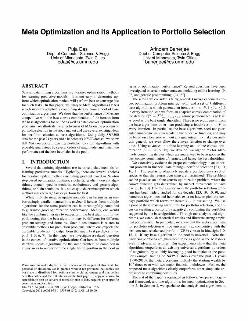
Figure 1: The best convex combination xwt of the iterates fromthe base algorithms is always better than individual iteratesxt,h(the red dot is the global minimum and the green dot isthe best point in the convex hull of iterates): (a) xwt achieves theglobal minimum, (b) xwt is on an edge of the hull, and (c) xwtoverlaps with the best iterate.

the problem of portfolio selection. We present comprehensive ex-perimental results in Section 4, and conclude in Section 5.

2. ONLINE META OPTIMIZATIONConsider the following generic convex optimization problem which

shows up while building models for a variety of data mining tasks[25]:

minx∈P

φ(x) , (1)

where φ is a convex function and P ∈ Rd determines the convexfeasible set. For the meta-optimization setting, we assume access tok different iterative algorithms A1, . . . , Ak, referred to as base al-gorithms, which attempt to solve the above problem. In particular,Ah is assumed to generate a feasible xt,h ∈ P at every iteration.The analysis we present does not depend on any other propertiesof the base algorithms or the iterates. The iterates may be comingfrom a iterative convex optimization routines based on gradient orNewton methods, from domain specific heuristics, or even entirelyarbitrary guesses. The proposed meta-algorithm picks a suitableiterate from the convex hull of the iterates at any time, given by:

Co(Xt) =

(Xtw =

kXh=1

whxt,h

˛˛kXh=1

wh = 1, wh ≥ 0

),

where Xt = [xt,1 · · · xt,k] ∈ Rd×k is the matrix of iterates. Let∆k denote the k-dimensional simplex. Then, it is easy to see thatthe best point xwt = Xtw =

Ph whxt,h ∈ Co(Xt) will always

achieve a lower (better) objective function value than any of theindividual iterates, i.e.,

minw∈∆k

φ

kXh=1

whxt,h

!≤ φ(xt,h), ∀h .

Figure 1 shows examples to illustrate the above point. In Fig-ure 1(a), the best point in the convex hull of the iterates achieves theglobal minimum of the function; in Figure 1(b), it is nearest to theglobal minimum; and in Figure 1(c), the best point in the convexhull is an iterate itself, i.e., a corner of the hull.

In general, the best point xwt = Xtw ∈ Co(Xt) inside the con-vex hull or equivalently the best convex combination w ∈ ∆k can-not be obtained in closed form. One can design optimization algo-rithms to find the best point inside the convex hull. Note that suchcomputations have to be repeated at every iteration, since corners ofthe hull, determined by Xt, changes in every iteration. In this sec-tion, we develop algorithms which adaptively pick wt ∈ ∆k based

Algorithm 1 Online Gradient Update (OGU) for Meta Optimiza-tion1: Initialize w1,h = 1

k, h = 1, . . . , k

2: For t = 1, . . . , T3: Receive Xt = [xt,1 · · · xt,k] from base algorithms4: Compute xwt

t =Pkh=1 wt,hxt,h

5: Receive convex function φt from nature6: Update distribution

wt+1,h = wt,h exp(−η`t(h))/Zt

where `t(h) is as in (6) and Zt is the partition function.

on Xt−1, and show that the iterates xwtt = Xtwt =

Ph wt,hxt,h

of the meta-algorithm are competitive with any fixed convex com-bination w ∈ ∆k used over iterations, i.e., ∀w ∈ ∆k we have

TXt=1

φ(Xtwt) ≤TXt=1

φ (Xtw) + o(T ) . (2)

In particular, if any w∗ ∈ ∆k achieves the global minimum, theadaptive approach will find the global minimum as well. Indeed,instead of simply being competitive with the single best iterate, theadaptive xwt

t will be competitive with any convex combinationsof them (Figure 1). To present our analysis in its full generality,we consider the online convex optimization (OCO) setting [28],where the convex function itself can change over time. We denotethe convex function at time t to be φt. Note that we can recoverthe batch case analysis for a fixed φ as a special case by simplysetting φt = φ, ∀t. In the OCO setting, we intend to get a set ofadaptive iterates xwt

t such that the following form of regret boundsare satisfied:

TXt=1

φt(Xtwt) ≤ minw∈∆k

TXt=1

φt (Xtwt) + o(T ) . (3)

2.1 Online Gradient UpdatesOur meta algorithm and analysis for Online Gradient Updates

(OGU) involves suitably reducing the Online Meta Optimization(OMO) problem to an online learning problem over k experts [22,9], where each expert corresponds to a corner for meta-optimization.We start by recalling a standard result from the online learning lit-erature [22, 12, 3]:

Lemma 1 Let `t ∈ [0, 1]k, t = 1, . . . , T, be an arbitrary sequenceof loss vectors over the k experts. If one maintains an adaptivedistribution over the experts using multiplicative updates given bypt+1(h) = pt(h) exp(−η`t(h))/Zt, where η > 0 and Zt is thepartition function, then for any w ∈ ∆k, the following inequalityholds:

TXt=1

pTt `t ≤ηPTt=1 w

T `t + log k

1− exp(−η). (4)

Variants of the above result form the basis of much work in onlinelearning, boosting, game theory, and numerous other developmentsin the past two decades [22, 12, 11, 2, 3, 9]. We now outline atransformation of the OMO problem to the above online learningsetting.

For our analysis, we assume that the sequence of convex func-tions φt can be arbitrary, but satisfies ‖∇φt(x)‖∞ ≤ g∞ for x ∈P . Further, we assume x ∈ P satisfies ‖x‖1 ≤ c. For the portfolio

selection application in Section 3, we will obtain specific values forg∞ and c. Let

ft(w) = φt (Xtw) . (5)

Since φt : P 7→ R, where P ⊆ Rd, is a convex function, thefunction ft : ∆k 7→ R is also convex. To see this, first note thatthe Hessian ∇2ft(w) = XT

t ∇2φt(Xtw)Xt. Since φt is convex,∇2φ(Xtw) is positive semi-definite. Hence, ∇2ft(w) is positivesemi-definite, implying convexity of ft. Define loss vector

`t =1

2

„∇ft(wt)cg∞

+ e

«∈ Rk , (6)

where e is the all ones vector. Based on this definition of loss, Algo-rithm 1 presents an adaptive algorithm for Online gradient updatefor meta optimization. We establish the following regret bound forOGO for this algorithm:

Theorem 1 For any sequence of convex functions φt such that‖∇φt(x)‖∞ ≤ g∞, and any sequence of iterates Xt = [xt,1 · · ·

· · · xt,k] such that ‖xt,h‖1 ≤ c, for η = log

„1 +

q2 log kT

«in

Algorithm 1, we have

TXt=1

ft(wt)− minw∈∆k

TXt=1

ft(w)

≤ 2cg∞“p

2T log k + log k”.

(7)

PROOF. Since ∇ft(wt) = XTt ∇φt(Xtwt), ‖∇ft(wt)‖∞ =

maxh |xTt,h∇φt(xwtt )|. From Hölder’s inequality [26, 14, 21],

|xTt,h∇φt(Xtwt)| ≤ ‖xt,h‖1‖∇φt(Xtwt)‖∞ ≤ cg∞ .

Hence ∇ft(wt)cg∞

∈ [−1, 1]k, so that `t ∈ [0, 1]k. From Lemma 1,Algorithm 1 will satisfy (4). Let ε = 1 − exp(−η) so that fromLemma 1 we have

TXt=1

wTt `t −TXt=1

wT `t ≤ εT +1

εlog k ,

where we have usedPtt=1 w

T `t ≤ T . Choosing ε =√

2 log k√2 log k+

√T

,a direct calculation shows

TXt=1

`Tt (wt − w) ≤p

2T log k + log k . (8)

Now, since ft is convex, we have

ft(wt)− ft(w) ≤ ∇ft(wt)T (wt − w) = 2cg∞`Tt (wt − w) ,

where the last equality follows since eT (wt − w) = 0 as wt, w ∈∆k. Adding over all t and using (8), we have

TXt=1

ft(wt)−TXt=1

ft(w) ≤ 2cg∞

TXt=1

`Tt (wt − w)

≤ 2cg∞“p

2T log k + log k”.

Noting that the above inequality holds for any w ∈ ∆k completesthe proof.

Since 2cg∞`√

2T log k + log k´

= o(T ), we have a desiredform of the bound. Further, assuming φt = φ gives the corre-sponding bound for the batch optimization case.

Algorithm 2 Online Newton Update (ONU) for Meta Optimization1: Initialize w1 ∈ ∆k

2: Let β = minn

18cg∞

, αo

3: For t = 1, . . . , T4: Receive Xt = [xt,1 · · · xt,k] from base algorithms5: Compute xwt

t =Pkh=1 wt,hxt,h

6: Receive convex function φt from nature7: Update distribution

wt+1,h =YAt

∆k

„wt −

2

βA−1t ∇ft

«,

where At andQAt

∆kare as in (9) and (10).

2.2 Online Newton UpdatesOur analysis for Online Newton Updates (ONU) build on recent

advances in Online Convex Optimization (OCO) [15, 1]. The anal-ysis of ONU differs from the standard analysis of online Newtonstep [15] due to two reasons: first, our analysis focuses on the de-rived convex function ft : ∆k 7→ R instead of the original convexfunction φt : P 7→ R, and second, our bounds are based on theL∞ norm of φt instead of the L2 norm, which can be substantiallylarger for high-dimensional problems.

Following [15], we consider convex functions φt which satisfythe α-exp-concavity property: there is a α > 0 such that for x ∈ P ,exp(−αφt(x)) is a concave function . Note that α-exp-concavefunctions φt are more general than ones which have bounded gra-dients and Hessians which are strictly bounded away from 0, i.e.,∇2φt � HI for some constant H > 0. As before, we assume thatL∞ norm of the gradient of φt are bounded above, i.e., ‖∇φt‖∞ ≤g∞.

With these assumptions, Algorithm 2 presents the Online New-ton Update (ONU) algorithm for Online Meta Optimization [15].In essence, the algorithm takes a Newton-like step from the currentiterate wt, and then projects the vector to the feasible set ∆k toobtain wt+1. Note that the algorithm does not use the actual Hes-sian of ft, but a matrix based on the outer product of the gradientsdefined as:

At =

tXτ=1

∇ft∇fTt + εI , (9)

where ε = kβ2c2

. FurtherQAt

∆kis the projection onto ∆k using the

Mahalanobis distance induced by At, i.e.,YAt

∆k

(w) = argminw∈∆k

(w − w)TA−1t (w − w) . (10)

We start our analysis by showing that if φt is α-exp-concave forx ∈ P , then ft is α-exp-concave for w ∈ ∆k for the same (set of)α.

Lemma 2 If φt is α-exp-concave for some α > 0, then ft as de-fined in (5) is also α-exp-concave.

PROOF. Let ht(w) = exp(−αft(w)). The Hessian is given by

∇2ht(w) = [α2(∇ft)(∇ft)T − α∇2ft]ht(w)

= XTt [α2(∇φt)(∇φt)T − α∇2φt]Xtht(w)

Let ψt(x) = exp(−αφt(x)). Since φt is α-exp-concave, the Hes-sian∇2ψt � 0, so that

[α2(∇φt)(∇φt)T − α∇2φt]ψt(x) � 0 .

LetBt = [α2(∇φt)(∇φt)T −α∇2φt]. Since ψt(x) ≥ 0, we have

Bt � 0 ⇒ XTt BtXt � 0 ,

so that∇2ht � 0 since ht(w) ≥ 0, implying ht isα-exp-concave.

We now establish a result, similar to Lemma 3 in [15], but usingthe L∞ bound g∞ and the fact that ‖x‖1 ≤ c for x ∈ P .

Lemma 3 For β ≤ min{ 18cg∞

, α}, for any w,wt ∈ ∆k, we have

ft(w) ≥ ft(wt) +∇ft(wt)T (w − wt)

+β

4(w − wt)T∇ft(wt)∇ft(wt)T (w − wt) .

(11)

PROOF. Since β ≤ α, following the proof of Lemma 3 in [15]we have

ft(w) ≥ ft(wt)−1

βlog[1− β∇ft(wt)T (w − wt)] .

Now, by Hölder’s inequality,

|β∇ft(wt)T (w−wt)| ≤ β‖∇ft(wt)‖∞‖w−wt‖1 ≤ 2βcg∞ ≤1

4.

Since − log(1 − z) ≥ z + 14z2 for |z| ≤ 1

4, using it for z =

β∇ft(wt)T (w − wt) completes the proof.

We now present the main result for ONU:

Theorem 2 For any sequence of α-exp-concave functions φt suchthat ‖∇φt‖∞ ≤ g∞ for x ∈ P where ‖x‖1 ≤ c, for T ≥ 2awhere a = 32g∞

c2, we have the following regret bound:

TXt=1

ft(wt)− minw∈∆k

TXt=1

ft(w) ≤ k„

8cg∞ +1

α

«log

eT

a. (12)

PROOF. Using Lemma 3 and using the proof of Theorem 2 in [15],we haveTXt=1

Rt ≤1

β

TXt=1

∇Tt A−1t ∇t+

β

4(wt−w)T (A1−∇1∇T1 )(w1−w) ,

where Rt = ft(wt) − ft(w) for any w ∈ ∆k, ∇t = ∇ft, andAt =

Ptτ=1∇τ∇

Tτ + εI as in (9). Since A1 − ∇1∇T1 = εI,

‖w1 − w‖22 ≤ 4c2, and ε = kβ2c2

, we have

TXt=1

Rt ≤1

β

TXt=1

∇Tt A−1t ∇t +

β

4ε‖w1 − w‖22

≤ 1

β

TXt=1

∇Tt A−1t ∇t +

k

β.

Since ‖∇ft‖ ≤√k‖∇ft‖∞ ≤

√kcg∞, from Lemma 11 in [15],

we haveTXt=1

∇Tt A−1t ∇t ≤ k log

„kc2g2

∞T

ε+ 1

«≤ k log

„T

2a+ 1

«,

where we have used ε = kβ2c2

, β ≤ 18cg∞

, and a = 32g∞c2

. ForT ≥ 2a, T

2a+ 1 ≤ T

a. Plugging everything back, we have

TXt=1

Rt ≤k

β

„log

T

a+ 1

«=k

βlog

eT

a.

Since β = min{ 18cg∞

, α}, we have

1

β= max

8cg∞,

1

α

ff≤ 8cg∞ +

1

α.

Plugging this upper bound back completes the proof.

3. META OPTIMIZATION FOR PORTFO-LIO SELECTION

We consider a stock market consisting of n stocks {s1, . . . , sn}over a span of T periods. For ease of exposition, we will con-sider a period to be a day, but the analysis presented in the paperholds for any valid definition of a ‘period,’ such as an hour or amonth. Let rt(i) denote the price relative of stock si in day t,i.e., the multiplicative factor by which the price of si changes inday t. Hence, rt(i) > 1 implies a gain, rt(i) < 1 implies a loss,and rt(i) = 1 implies the price remained unchanged. We assumert(i) > 0 for all i, t. Let rt = 〈rt(1), . . . , rt(n)〉 denote the vec-tor of price relatives for day t, and let r1:t denote the collection ofsuch price relative vectors upto and including day t. A portfolioxt = 〈xt(1), . . . , xt(n)〉 on day t can be viewed as a probabilitydistribution over the stocks that prescribes investing xt(i) fractionof the current wealth in stock st(i). Note that the portfolio xt hasto be decided before knowing rt which will be revealed only at theend of the day. The multiplicative gain in wealth at the end of dayt, is then simply rTt xt =

Pni=1 rt(i)xt(i). Given a sequence of

price relatives r1:t−1 = {r1, . . . , rt−1} upto day (t − 1), the se-quential portfolio selection problem in day t is to determine a port-folio xt based on past performance of the stocks. At the end of dayt, rt is revealed and the actual performance of xt gets determinedby rTt xt. Over a period of T days, for a sequence of portfoliosx1:T = {x1, . . . , xt}, the multiplicative gain in wealth is then

S(x1:T , r1:T ) =

TYt=1

“rTt xt

”. (13)

The above problem can be viewed as an Online Convex Optimiza-tion (OCO), where the convex function φt(xt) = − log(rTt xt),and the cumulative loss over T iterations is

TXt=1

φt(xt) = −TXt=1

log(rTt xt) = − logS(x1:T , r1:T ) . (14)

There are numerous algorithms in the literature for picking the port-folio xt on a given day based on past information r1:(t−1) [10, 16,9, 1, 5]. Instead of proposing new algorithms for the task, we focuson meta optimization to combine the portfolios from a pool of basealgorithms from the literature. We now specialize the general caseresults and algorithms of Section 2 to the task of portfolio selection.

Consider k base algorithms {A1, . . . , Ak} for portfolio selec-tion where algorithm Ah generates a portfolio xt,h ∈ ∆n basedon the past information r1:(t−1). Recall that our analysis doesnot impose any other constraints on the base algorithms and sothey can be based on theoretically well grounded ideas [10, 16,1] or good heuristics [5]. Given the set of base portfolios Xt =[xt,1 · · · xt,k], the goal of the meta algorithm is to choose wt ∈∆k to construct the portfolio xwt

t = Xtwt and subsequently in-cur loss ft(wt) = φt(x

wtt ) = − log(rTt x

wtt ) = − log(rTt Xtwt).

Since a portfolio x ∈ ∆n, we have c = ‖x‖1 = 1. Among allprice relatives over all stocks, let rmin = mini,t rt(i) > 0 and letrmax = maxi,t rt(i). Since ∇φt(x) = − rt

rTt x

, ‖∇φt(x)‖∞ ≤rmaxrmin

= g∞. For convenience, we use u = rmaxrmin

. For our subse-

quent analysis, we note that

∇ft(wt) = − XTt rt

rTt Xtwt. (15)

Gradient Updates: Since ∇φt(x) for portfolio selection is a pos-itive vector, one can define the loss vector for OGU in Algorithm 1as follows:

`t =∇ft(wt)cg∞

= − 1

2u

XTt rt

rTt Xtwt+ e . (16)

With this modification, the OGU in Algorithm 1 has the followingguarantee:

Corollary 1 For any sequence of price relatives r1:T and any se-quence of base portfolios X1:T , the log-wealth accumulated byAlgorithm 1 choosing adaptive wt satisfies the following regretbound:

maxw∈∆k

TXt=1

log(rTt Xtw)−TXt=1

log(rTt Xtwt)

≤ u“p

2T log k + log k”.

(17)

The proof follows from a direct application of Theorem 1. Webriefly discuss the implication of the fact that the wealth accumu-lated by the adaptive meta algorithm will be competitive with anyfixed combination strategy chosen in hindsight. If one of the basealgorithms is universal [10, 16, 4, 17, 9], i.e., competitive with bestconstant rebalanced portfolio (CRP) [10, 4] in hindsight so that

maxx∈∆n

TXt=1

log(rTt x)−TXt=1

log(rTt xt) = o(T ) , (18)

then our meta algorithm will also be universal. Also, since the bestCRP would outperform the best stock, having an universal algo-rithm in the pool is sufficient to ensure the meta algorithm will becompetitive with the single best stock in hindsight. More generally,the meta algorithm will be competitive with the best convex combi-nation of the base algorithms, which is guaranteed to be better thanthe best base algorithm in the pool (Figure 1).

Newton Updates: We start our analysis with the following result:

Lemma 4 φt(x) = − log(rTt x) is a α-exp-concave function forα ∈ (0, 1].

PROOF. Let ψt(x) = exp(−αφt(x)) = (rTt x)α. A direct cal-culation shows the Hessian to be

∇2ψt(x) = α(α− 1)rtr

Tt

rTt xψt(x) ,

which is negative semi-definite for α > 0 if α ∈ (0, 1].As a result, Algorithm 2 can be applied as a meta algorithm for

the portfolio selection problem. As before, c = 1, g∞ = u. Choos-ing α = 1, β = min{ 1

8u, α} = 1

8usince u = rmax

rmin≥ 1. Hence,

1β

= 8u. Further, a = 32g∞c2

= 32u, so that ae≤ 12u. Us-

ing the above values in Algorithm 2, from Theorem 2 we have thefollowing result:

Corollary 2 For any sequence of price relatives r1:T and any se-quence of base portfolios X1:t, the log-wealth accumulated by Al-

gorithm 2 choosing adaptivewt satisfies the following regret bound:

maxw∈∆k

TXt=1

log(rTt Xtw)−TXt=1

log(rTt Xtwt) ≤ 8ku logT

12u.

(19)

As before, the proof follows from a direct application of Theo-rem 2. The bound has the same optimality properties as discussedin the context of OGU above. In fact, the worst case regret ofONU grows as O(log T ) as opposed to O(

√T ) for OGU. The

bound for OGU can in fact be sharpened in this setting by suit-ably modifying the OGU algorithm and analysis using the fact thatthe Hessian ∇2ft is bounded away from 0 under the assumptionmini,t ri,t > 0.

4. EXPERIMENTAL RESULTSWe conducted extensive experiments on two financial data-sets

to establish how effective Online Meta Optimization can be carriedout by OGU and ONU. In this section, we describe the datasetsthat were chosen for the experiments, the algorithms, the parameterchoices and most importantly the results of our experiments.Datasets: The experiments were conducted on two major datasets:the New York Stock Exchange dataset (NYSE) [10] and a Standard& Poor’s 500 (S&P 500) dataset. The NYSE dataset consists of 36stocks with data accumulated over a period of 22 years from July3, 1962 to Dec 31 1984. The dataset captures the bear market thatlasted between January 1973 and December 1974. However, all ofthe 36 stocks increase in value in the 22-year run.

The S&P500 dataset that we used for our experiments consists of263 stocks which were present in the S&P500 index in December2010 and were alive since January 1990. This period of 21 yearsfrom 1990 to 2010 covers bear and bull markets of recent times.Methodology: We ran a pool of base portfolio selection algorithmsand the Meta Algorithms on the datasets (NYSE and S&P500). Forour experiments, this pool included universal and non-universal al-gorithms. We start by briefly describing the base algorithms andthe Meta Algorithms.

4.1 Base AlgorithmsOf the base algorithms that we used for our experiments UP, EG

and ONS are universal while Anticor and its variant are heuristics.Universal Portfolios (UP):The key idea behind Cover’s [10] UP isto maintain a distribution over all Constant Rebalanced Portfolios(CRPs) and perform a Bayesian update after observing every rt.Each CRP q is a distribution over n stocks and hence lies in then-simplex, one uses a distribution µ(q) over the n-simplex. Theuniversal portfolio xt is defined as:

xt(i) =

Rqq(i)St−1(q, r1:t−1)µ(q)dqRqSt−1(q, r1:t−1)µ(q)dq

. (20)

UP has a regret of O(log T ) with respect to the best CRP in hind-sight. However, the updates for UP are computationally prohibitive.Exponentiated Gradient (EG): Exponentiated Gradient (EG) [16]scales linearly with the number of stocks but is weaker in regretthan UP. The EG investment strategy was introduced and analyzedby [16]. At the start of day t, the algorithm computes its new port-folio vector xt such that it stays close to xt−1 and does well onthe price relatives rt−1 for the previous day. The updated portfolioturns out to be

xt(i) =xt−1(i) exp(ηrt−1(i)/xTt−1rt−1)Pn

i′=1 xt−1(i′) exp(ηrt−1(i′)/xTt−1rt−1). (21)

’62 ’64 ’66 ’68 ’70 ’72 ’74 ’76 ’78 ’80 ’82 ’8410

−1

100

101

102

103

Year

Lo

gari

thm

ic W

ealt

h G

row

th

Monetary returns on the NYSE dataset

UP

EG

ONS

UCRPMA

EG

MAONS

(a) Monetary returns on NYSE.

‘90‘91‘92‘93 ‘94 ‘95 ‘96 ‘97 ‘98 ‘99 ‘00 ‘01 ‘02 ‘03 ‘04 ‘05 ‘06 ‘07 ‘08 ‘09 ‘1010

−1

100

101

102

103

104

Year

Lo

gari

thm

ic W

ealt

h G

row

th

Monetary returns on the S&P500 dataset

UP

EG

ONS

UCRPMA

EG

MAONS

(b) Monetary returns on S&P500.

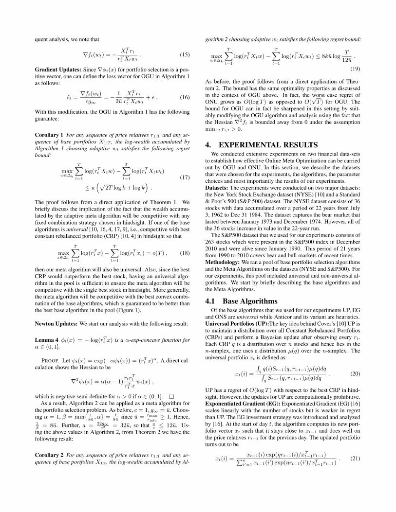
Figure 2: Monetary returns of the Meta Algorithms, MA EG and MA ONS for $1 investment, is competitive with the best performingbase algorithm ONS in this case(best viewed in color).

’62 ’64 ’66 ’68 ’70 ’72 ’74 ’76 ’78 ’80 ’82 ’8410

−2

100

102

104

106

Year

Lo

gari

thm

ic W

ealt

h G

row

th

Monetary returns on the NYSE dataset

UP

EG

ONSAnticor

30

UCRPMA

EG

MAONS

(a) Monetary returns on NYSE.

‘90‘91‘92‘93 ‘94 ‘95 ‘96 ‘97 ‘98 ‘99 ‘00 ‘01 ‘02 ‘03 ‘04 ‘05 ‘06 ‘07 ‘08 ‘09 ‘1010

−1

100

101

102

103

104

Year

Lo

gari

thm

ic W

ealt

h G

row

th

Monetary returns on the S&P500 dataset

UP

EG

ONSAnticor

30

UCRPMA

EG

MAONS

(b) Monetary returns on S&P500.

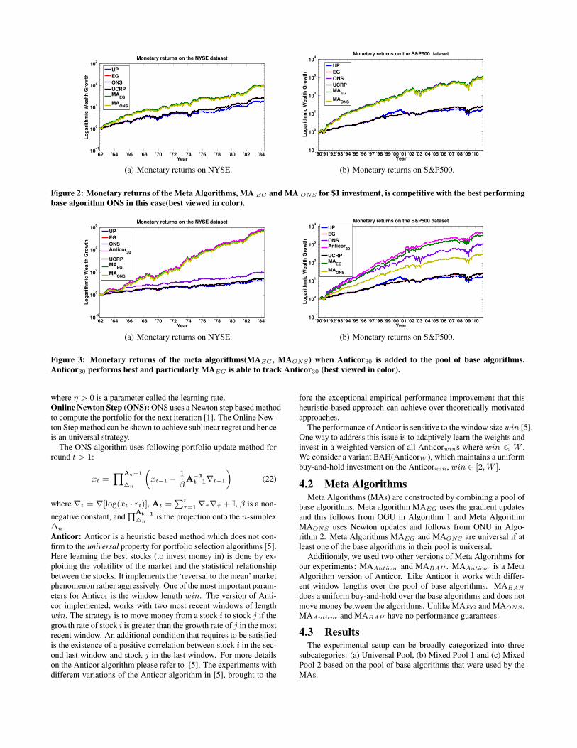
Figure 3: Monetary returns of the meta algorithms(MAEG, MAONS) when Anticor30 is added to the pool of base algorithms.Anticor30 performs best and particularly MAEG is able to track Anticor30 (best viewed in color).

where η > 0 is a parameter called the learning rate.Online Newton Step (ONS): ONS uses a Newton step based methodto compute the portfolio for the next iteration [1]. The Online New-ton Step method can be shown to achieve sublinear regret and henceis an universal strategy.

The ONS algorithm uses following portfolio update method forround t > 1:

xt =YAt−1

∆n

„xt−1 −

1

βA−1

t−1∇t−1

«(22)

where∇t = ∇[log(xt · rt)], At =Ptτ=1∇τ∇τ + I, β is a non-

negative constant, andQAt−1

4nis the projection onto the n-simplex

∆n.Anticor: Anticor is a heuristic based method which does not con-firm to the universal property for portfolio selection algorithms [5].Here learning the best stocks (to invest money in) is done by ex-ploiting the volatility of the market and the statistical relationshipbetween the stocks. It implements the ‘reversal to the mean’ marketphenomenon rather aggressively. One of the most important param-eters for Anticor is the window length win. The version of Anti-cor implemented, works with two most recent windows of lengthwin. The strategy is to move money from a stock i to stock j if thegrowth rate of stock i is greater than the growth rate of j in the mostrecent window. An additional condition that requires to be satisfiedis the existence of a positive correlation between stock i in the sec-ond last window and stock j in the last window. For more detailson the Anticor algorithm please refer to [5]. The experiments withdifferent variations of the Anticor algorithm in [5], brought to the

fore the exceptional empirical performance improvement that thisheuristic-based approach can achieve over theoretically motivatedapproaches.

The performance of Anticor is sensitive to the window sizewin [5].One way to address this issue is to adaptively learn the weights andinvest in a weighted version of all Anticorwins where win 6 W .We consider a variant BAH(AnticorW ), which maintains a uniformbuy-and-hold investment on the Anticorwin, win ∈ [2,W ].

4.2 Meta AlgorithmsMeta Algorithms (MAs) are constructed by combining a pool of

base algorithms. Meta algorithm MAEG uses the gradient updatesand this follows from OGU in Algorithm 1 and Meta AlgorithmMAONS uses Newton updates and follows from ONU in Algo-rithm 2. Meta Algorithms MAEG and MAONS are universal if atleast one of the base algorithms in their pool is universal.

Additionaly, we used two other versions of Meta Algorithms forour experiments: MAAnticor and MABAH . MAAnticor is a MetaAlgorithm version of Anticor. Like Anticor it works with differ-ent window lengths over the pool of base algorithms. MABAHdoes a uniform buy-and-hold over the base algorithms and does notmove money between the algorithms. Unlike MAEG and MAONS ,MAAnticor and MABAH have no performance guarantees.

4.3 ResultsThe experimental setup can be broadly categorized into three

subcategories: (a) Universal Pool, (b) Mixed Pool 1 and (c) MixedPool 2 based on the pool of base algorithms that were used by theMAs.

’62 ’64 ’66 ’68 ’70 ’72 ’74 ’76 ’78 ’80 ’82 ’8410

−2

100

102

104

106

108

Year

Lo

gari

thm

ic W

ealt

h G

row

th

Monetary returns on the NYSE dataset

UP

EG

ONSAnticor

30

BAH(Anticor30

)

UCRPMA

EG

MAONS

(a) Monetary returns on NYSE.

‘90‘91‘92‘93 ‘94 ‘95 ‘96 ‘97 ‘98 ‘99 ‘00 ‘01 ‘02 ‘03 ‘04 ‘05 ‘06 ‘07 ‘08 ‘09 ‘1010

−2

100

102

104

106

Year

Lo

gari

thm

ic W

ealt

h G

row

th

Monetary returns on the S&P500 dataset

UP

EG

ONS

Anticor30

BAH(Anticor30

)

UCRP

(b) Monetary returns on S&P500.

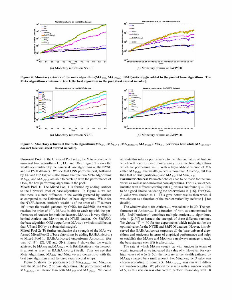
Figure 4: Monetary returns of the meta algorithms(MAEG, MAONS). BAH(Anticor30)is added to the pool of base algorithms. TheMeta Algorithms continue to track the best algorithm in the pool.(best viewed in color).

’62 ’64 ’66 ’68 ’70 ’72 ’74 ’76 ’78 ’80 ’82 ’8410

−2

100

102

104

106

108

Year

Lo

gari

thm

ic W

ealt

h G

row

th

Monetary returns on the NYSE dataset

UP

EG

ONSAC

30

BAH(Anticor30

)

UCRPMA

EG

MAONS

MAAC

5

MABAH

(a) Monetary returns on NYSE.

‘90‘91‘92‘93 ‘94 ‘95 ‘96 ‘97 ‘98 ‘99 ‘00 ‘01 ‘02 ‘03 ‘04 ‘05 ‘06 ‘07 ‘08 ‘09 ‘1010

−2

100

102

104

106

Year

Lo

gari

thm

ic W

ealt

h G

row

th

Monetary returns on the SP500 dataset

UP

EG

ONSAnticor

30

BAH(Anticor30

)

UCRPMA

EG

MAONS

MAAnticor

5

MABAH

(b) Monetary returns on S&P500.

Figure 5: Monetary returns of the meta algorithms(MAEG, MAONS , MAAnticor , MABAH ). MAEG performs best while MAAnticordoesn’t fare well.(best viewed in color).

Universal Pool: In the Universal Pool setup, the MAs worked withuniversal base algorithms UP, EG, and ONS. Figure 2 shows thewealth accumulated by the universal base algorithms on the NYSEand S&P500 datasets. We see that ONS performs best, followedby EG and UP. Figure 2 also shows that the two Meta AlgorithmsMAEG and MAONS are able to catch up with the performance ofONS, the best performing algorithm in the pool.Mixed Pool 1: The Mixed Pool 1 is formed by adding Anticorto the Universal Pool of base algorithms. In Figure 3, we seethat there is a stark difference in the wealth garnered by Anticoras compared to the Universal Pool of base algorithms. While forthe NYSE dataset, Anticor’s wealth is of the order of 106 (almost104 times the wealth gathered by ONS), for S&P500, the wealthreaches the order of 103. MAEG is able to catch up with the per-formance of Anticor for both the datasets. MAONS is very slightlybehind Anticor and MAEG on the NYSE dataset. On S&P500,the base algorithm ONS outperforms MAONS (which is still betterthan UP and EG by a sybstantial margin).Mixed Pool 2: To further emphasize the strength of the MAs weformed Mixed Pool 2 of base algorithms by adding BAH(AnticorW )to Mixed Pool 1. BAH(AnticorW ) outperforms Anticorwin (forwin 6 W ), EG, UP, and ONS. Figure 4 shows that the wealthachieved by MAEG and MAONS with BAH(AnticorW ) in the pool,is almost as much as BAH(AnticorW ) itself. Thus we see thatMeta Algorithms, MAEG and MAONS are competitive with thebest base algorithm in all the three experimental setups.

Figure 5, shows the performance of MAAnticor and MABAHwith the Mixed Pool 2 of base algorithms. The performance of theMAAnticor is inferior than both MAEG and MAONS . We could

attribute this inferior performance to the inherent nature of Anticorwhich will tend to move money away from the base algorithmswhich are performing well. With a buy-and-hold version of MAcalled MABAH , the wealth gained is more than Anticorw, but lessthan that of BAH(AnticorW ) and MAEG and MAONS .Parameter choices: Parameter choices had to be made for the uni-versal as well as non-universal base algorithms. For EG, we exper-imented with different learning rate (η) values and found η = 0.05to be a good choice, validating the observations in [16]. For ONS,β value was chosen as 1. This gave better results than when βwas chosen as a function of the market-variability (refer to [1] fordetails).

The window size w for Anticorwin was taken to be 30. The per-formance of Anticorwin is a function of win as demonstrated in[5]. BAH(AnticorW ) combines multiple Anticorwin algorithms,win ∈ [2,W ] to harness the strength of these different versions.We choose W = 30 for our experiments which might not be theoptimal value for the NYSE and S&P500 datasets. Hoever, it is ob-served that BAH(Anticor30) surpasses all the base universal algo-rithms and Anticor30 in terms of empirical performance and helpsus establish that MAEG and MAONS can always manage to trackthe best strategy even if it is a heuristic.

The rate at which MAEG caught up with Anticor in terms ofwealth increased as we increased the value of η. However, for veryhigh values of η (η > 50), the increase in the wealth gathered byMAEG changed by a small amount. For MAONS , the β value waschosen according to Lemma 3. MAAnticor was run with differ-ent window lengths. We plotted the results with a window lengthof 5, as this version was observed to perform reasonably well. It

12/1984

06/1974

06/1966

Weights by MAEG

on EG, ONS and AC with η=0.5

07/1962

07/1970

EG

ONS

AC

(a) NYSE: weights of MAEG with η=0.5.

01/200512/2001

12/1997

12/2010

Weights of MAEG

on EG, ONS and AC with η=1

12/1993

01/1990

AC

EG

ONS

(b) S&P500: weights of MAEG with η=1.

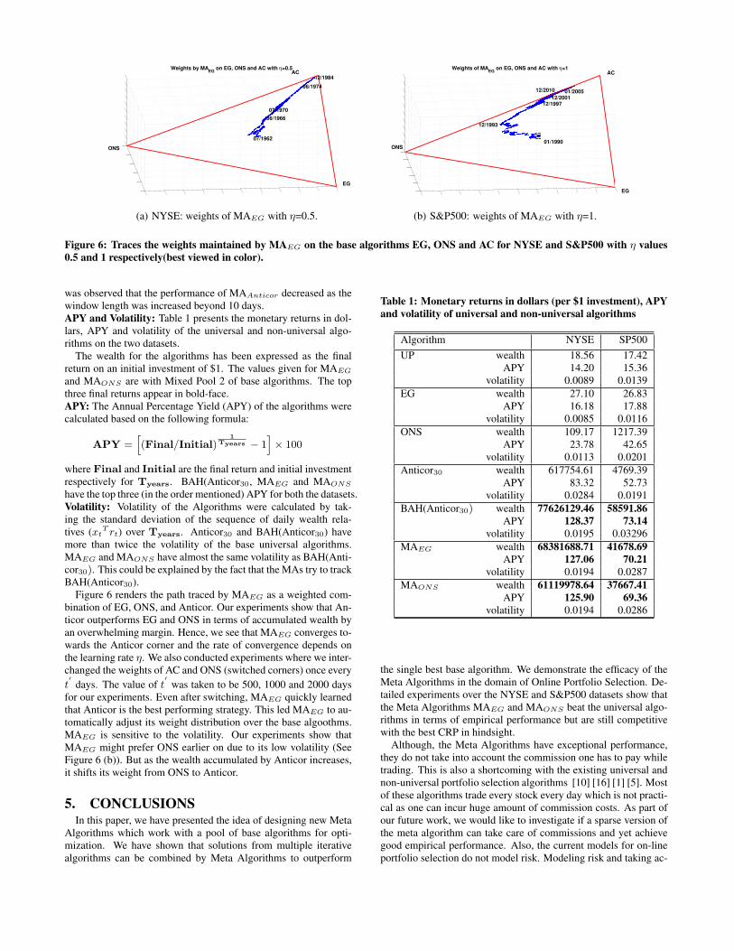
Figure 6: Traces the weights maintained by MAEG on the base algorithms EG, ONS and AC for NYSE and S&P500 with η values0.5 and 1 respectively(best viewed in color).

was observed that the performance of MAAnticor decreased as thewindow length was increased beyond 10 days.APY and Volatility: Table 1 presents the monetary returns in dol-lars, APY and volatility of the universal and non-universal algo-rithms on the two datasets.

The wealth for the algorithms has been expressed as the finalreturn on an initial investment of $1. The values given for MAEGand MAONS are with Mixed Pool 2 of base algorithms. The topthree final returns appear in bold-face.APY: The Annual Percentage Yield (APY) of the algorithms werecalculated based on the following formula:

APY =h(Final/Initial)

1Tyears − 1

i× 100

where Final and Initial are the final return and initial investmentrespectively for Tyears. BAH(Anticor30, MAEG and MAONShave the top three (in the order mentioned) APY for both the datasets.Volatility: Volatility of the Algorithms were calculated by tak-ing the standard deviation of the sequence of daily wealth rela-tives (xtT rt) over Tyears. Anticor30 and BAH(Anticor30) havemore than twice the volatility of the base universal algorithms.MAEG and MAONS have almost the same volatility as BAH(Anti-cor30). This could be explained by the fact that the MAs try to trackBAH(Anticor30).

Figure 6 renders the path traced by MAEG as a weighted com-bination of EG, ONS, and Anticor. Our experiments show that An-ticor outperforms EG and ONS in terms of accumulated wealth byan overwhelming margin. Hence, we see that MAEG converges to-wards the Anticor corner and the rate of convergence depends onthe learning rate η. We also conducted experiments where we inter-changed the weights of AC and ONS (switched corners) once everyt′

days. The value of t′

was taken to be 500, 1000 and 2000 daysfor our experiments. Even after switching, MAEG quickly learnedthat Anticor is the best performing strategy. This led MAEG to au-tomatically adjust its weight distribution over the base algoothms.MAEG is sensitive to the volatility. Our experiments show thatMAEG might prefer ONS earlier on due to its low volatility (SeeFigure 6 (b)). But as the wealth accumulated by Anticor increases,it shifts its weight from ONS to Anticor.

5. CONCLUSIONSIn this paper, we have presented the idea of designing new Meta

Algorithms which work with a pool of base algorithms for opti-mization. We have shown that solutions from multiple iterativealgorithms can be combined by Meta Algorithms to outperform

Table 1: Monetary returns in dollars (per $1 investment), APYand volatility of universal and non-universal algorithms

Algorithm NYSE SP500UP wealth 18.56 17.42

APY 14.20 15.36volatility 0.0089 0.0139

EG wealth 27.10 26.83APY 16.18 17.88

volatility 0.0085 0.0116ONS wealth 109.17 1217.39

APY 23.78 42.65volatility 0.0113 0.0201

Anticor30 wealth 617754.61 4769.39APY 83.32 52.73

volatility 0.0284 0.0191BAH(Anticor30) wealth 77626129.46 58591.86

APY 128.37 73.14volatility 0.0195 0.03296

MAEG wealth 68381688.71 41678.69APY 127.06 70.21

volatility 0.0194 0.0287MAONS wealth 61119978.64 37667.41

APY 125.90 69.36volatility 0.0194 0.0286

the single best base algorithm. We demonstrate the efficacy of theMeta Algorithms in the domain of Online Portfolio Selection. De-tailed experiments over the NYSE and S&P500 datasets show thatthe Meta Algorithms MAEG and MAONS beat the universal algo-rithms in terms of empirical performance but are still competitivewith the best CRP in hindsight.

Although, the Meta Algorithms have exceptional performance,they do not take into account the commission one has to pay whiletrading. This is also a shortcoming with the existing universal andnon-universal portfolio selection algorithms [10] [16] [1] [5]. Mostof these algorithms trade every stock every day which is not practi-cal as one can incur huge amount of commission costs. As part ofour future work, we would like to investigate if a sparse version ofthe meta algorithm can take care of commissions and yet achievegood empirical performance. Also, the current models for on-lineportfolio selection do not model risk. Modeling risk and taking ac-

count of volatility of stocks is an interesting direction for our futurework.Acknowledgements: The research was supported by NSF CA-REER award IIS-0953274, and NSF grants IIS-0916750, IIS-08121-83, IIS-1029711, and NetSE-1017647. The authors also wish tothank Huahua Wang and Padmanabhan Balasubramanian for theirhelp.

6. REFERENCES

[1] A. Agarwal, E. Hazan, S. Kale, and R. Schapire. Algorithmsfor portfolio management based on the newton method.Proceedings of the 23rd International Conference onMachine Learning, pages 9–16, 2006.

[2] S. Arora, E. Hazan, and S. Kale. The multiplicative updatealgorithm: A meta algorithm and applications. Technicalreport, Dept of Computer Science, Princeton University,2005.

[3] A. Banerjee. On Bayesian bounds. In Proceedings of the23rd International Conference on Machine Learning, 2006.

[4] A. Blum and A. Kalai. Universal portfolios with and withouttransaction costs. In Proceedings of the 10th AnnualConference on Learning Theory, 1997.

[5] A. Borodin, R. El-Yaniv, and V. Gogan. Can we learn to beatthe best stock. Journal of Artificial Intelligence Research,21:579–594, 2004.

[6] L. Breiman. Bagging predictors. Machine Learning,24:123–140, 1996.

[7] L. Breiman. Random forests. Machine Learning, 45:5–32,2001.

[8] N. Cesa-Bianchi, Y. Freund, D. P. Helmbold, D. Haussler,R. Schapire, and M. K. Warmuth. How to use expert advice.Journal of the ACM, 44(3):427–485, 1997.

[9] N. Cesa-Bianchi and G. Lugosi. Prediction, Learning, andGames. Cambridge University Press, 2006.

[10] T. Cover. Universal portfolios. Mathematical Finance,1:1–29, 1991.

[11] Y. Freund and R. Schapire. Adaptive game playing usingmultiplicative weights. Games and Economic Behavior,29:79–103, 1999.

[12] Y. Freund and R. E. Schapire. A decision-theoreticgeneralization of on-line learning and an application toboosting. Journal of Computer and System Sciences,55(1):119–139, 1997.

[13] J. Friedman, T. Hastie, and R. Tibshirani. Additive logisticregression: A statistical view of boosting. Annals ofStatistics, 2000.

[14] B. Fristedt and L. Gray. A Modern Approach to ProbabilityTheory. Birkhauser Verlag, 1997.

[15] E. Hazan, A. Agarwal, and S. Kale. Logarithmic regretalgorithms for online convex optimization. MachineLearning, 69(2-3):169–192, 2007.

[16] D. Helmbold, E. Scahpire, Y. Singer, and M. Warmuth.Online portfolio setection using multiplicative weights.Mathematical Finance, 8(4):325–347, 1998.

[17] A. Kalai and S. Vempala. Efficient algorithms for universalportfolios. Journal of Machine Learning Research,3(3):423–440, 2002.

[18] A. Kalai and S. Vempala. Efficient algorithms for on-lineoptimization. Journal of Computer and System Sciences,713:291–307, 2005.

[19] J. L. Kelly. A new interpretation of information rate. BellSystems Technical Journal, 35:917–926, 1956.

[20] J. Kivinen and M. Warmuth. Exponentiated gradient versusgradient descent for linear predictors. Information andComputation, 132(1):1–64, 1997.

[21] O. Knill. Probability. Course notes from Caltech, 1994.[22] N. Littlestone and M. Warmuth. The weighted majority

algorithm. Information and Computation, 108:212–261,1994.

[23] H. Markowitz. Portfolio selection. Journal of Finance,7:77–91, 1952.

[24] T. Soule. Voting teams: A cooperative approach tonon-typical problems. Proceedings of the Genetic andEvolutionary Computation Conference, pages 916–922,1999.

[25] P. Tan, M. Steinbach, and V. Kumar. Introduction to DataMining, (First Edition). 2005.

[26] D. Williams. Probability with Martingales. CambridgeUniversity Press, 1991.

[27] W. Yan, M. Sewell, and C. D. Clack. Learning to optimizeprofits beats predicting returns – comparing techniques forfinancial portfolio optimisation. Proceedings of the Geneticand Evolutionary Computation Conference, pages1681–1688, 2008.

[28] Martin Zinkevich. Online convex programming andgeneralized infinitesimal gradient ascent. Proceedings of the20th International Conference on Machine Learning, 2003.