Embed Size (px)
Citation preview

International Journal of Psychological Research, 2010. Vol. 3. No. 1. ISSN impresa (printed) 2011-2084 ISSN electrónica (electronic) 2011-2079
Sánchez-Meca, J., Marín-Martínez, F., (2010). Meta-analysis in Psychological Research. International Journal of Psychological Research, 3 (1), 151-163.
International Journal of Psychological Research 151
Meta-analysis in Psychological Research.
El meta-análisis en la investigación psicológica.
Julio Sánchez-Meca and Fulgencio Marín-Martínez
University of Murcia, Spain
ABSTRACT
Meta-analysis is a research methodology that aims to quantitatively integrate the results of a set of empirical
studies about a given topic. With this purpose, effect-size indices are obtained from the individual studies and the
characteristics of the studies are coded in order to examine their relationships with the effect sizes. Statistical analysis in
meta-analysis requires the weighting of each effect estimate as a function of its precision, by assuming a fixed- or a random-
effects model. This paper outlines the steps required for carrying out the statistical analyses in a meta-analysis, the different
statistical models that can be assumed, and the consequences of the assumptions in interpreting their results. The statistical
analyses are illustrated with a real example.
Key words: Meta-analysis, effect size, fixed-effects models, random-effects models, mixed-effects models.
RESUME�
El meta-análisis es una metodología de investigación que pretende integrar cuantitativamente los resultados de un
conjunto de estudios empíricos sobre un determinado problema. Con este propósito, se calculan índices del tamaño del
efecto y se codifican las características de los estudios con objeto de examinar su relación con los tamaños del efecto. El
análisis estadístico en meta-análisis requiere ponderar cada estimación del efecto en función de su precisión asumiendo un
modelo de efectos fijos o de efectos aleatorios. En este trabajo se presentan las etapas necesarias para realizar un meta-
análisis, los diferentes modelos estadísticos que pueden asumirse y las consecuencias de asumir dichos modelos en la
interpretación de sus resultados. Finalmente, los análisis estadísticos se ilustran con datos de un ejemplo real.
Palabras clave: Meta-análisis, tamaño del efecto, modelos de efectos fijos, modelos de efectos aleatorios, modelos de
efectos mixtos.
Article received/Artículo recibido: December 15, 2009/Diciembre 15, 2009, Article accepted/Artículo aceptado: March 15, 2010/Marzo 15/2010 Dirección correspondencia/Mail Address: Julio Sánchez-Meca, Dpto. Psicología Básica y Metodología, Facultad de Psicología, Campus de Espinardo, Universidad de Murcia, 30100-Murcia, Spain, E-mail: [email protected] Fulgencio Marín-Martínez, University of Murcia, Spain
INTERNATIONAL JOURNAL OF PSYCHOLOGICAL RESEARCH esta incluida en PSERINFO, CENTRO DE INFORMACION PSICOLOGICA DE COLOMBIA, OPEN JOURNAL SYSTEM, BIBLIOTECA VIRTUAL DE PSICOLOGIA (ULAPSY-BIREME), DIALNET y GOOGLE SCHOLARS. Algunos de sus articulos aparecen en SOCIAL SCIENCE RESEARCH NETWORK y está en proceso de inclusion en diversas fuentes y bases de datos internacionales. INTERNATIONAL JOURNAL OF PSYCHOLOGICAL RESEARCH is included in PSERINFO, CENTRO DE INFORMACIÓN PSICOLÓGICA DE COLOMBIA, OPEN JOURNAL SYSTEM, BIBLIOTECA VIRTUAL DE PSICOLOGIA (ULAPSY-BIREME ), DIALNET and GOOGLE SCHOLARS. Some of its articles are in SOCIAL SCIENCE RESEARCH NETWORK, and it is in the process of inclusion in a variety of sources and international databases.
International Journal of Psychological Research, 2010. Vol. 3. No. 1. ISSN impresa (printed) 2011-2084 ISSN electrónica (electronic) 2011-2079
Sánchez-Meca, J., Marín-Martínez, F., (2010). Meta-analysis in Psychological Research. International Journal of Psychological Research, 3 (1), 151-163.
152 International Journal of Psychological Research
Meta-analysis in Psychological Research
1. Introduction
In the last 30 years meta-analysis has become a very useful methodological tool for accumulating research
on a given topic. The huge growth of research in
psychology has made it very difficult to synthesize the
results in any field without the help of statistical methods to
summarize the evidence. Unlike traditional reviews on a given topic, which are essentially subjective in nature,
meta-analysis aims to imbue the research review with the
same scientific rigor that is demanded of empirical studies:
objectivity, systematization and replicability. Thus, meta-
analysis is a method used to quantitatively integrate the
results of a set of empirical studies on a given research question. With this purpose, the results of each individual
study included in a meta-analysis have to be quantified in
the same metric, usually by calculating an effect-size index,
and then the effect estimates are statistically analyzed in
order to: (a) obtain an average estimate of the effect
magnitude, (b) assess heterogeneity among the effect
estimates, and (c) search for characteristics of the studies
that can explain the heterogeneity (Cooper, 2010; Cooper,
Hedges, & Valentine, 2009; Hunter & Schmidt, 2004;
Lipsey & Wilson, 2001; Petticrew & Roberts, 2006).
As meta-analysis aims to integrate single studies, the analysis unit is not the participant, but the single study.
Therefore, the sample size in a meta-analysis is the number
of studies that it has been possible to recover regarding the
research question.
Meta-analysis is being applied in many different
fields in psychology, but especially in evaluating the
effectiveness of treatments, interventions, and prevention
programs in such settings as mental health, education,
social services, or human resources. Other psychological
fields where meta-analysis is also being applied include areas such as gender differences in childhood, adolescence
or with adults of many aptitudes and attitudes;
psychometric validity of employment tests, and reliability
generalization of psychological tests in general (Cook,
Cooper, Cordray et al., 1992). Nowadays, it is very
common to find meta-analytic studies on very different topics in any scientific psychology journal. Therefore,
clinicians and researchers should have a sufficient
knowledge base for correctly interpreting and/or carrying
out meta-analyses.
This article is divided into four sections. Firstly,
the phases in which a meta-analysis is carried out are
presented. Then we outline the main statistical methods in
meta-analysis. In the next section statistical methods for
meta-analysis are illustrated using a real example. Finally,
we present some concluding remarks.
2. Phases in a Meta-analysis
A meta-analysis is a scientific investigation and,
consequently, it involves carrying out the same phases as in an empirical study. However, some of the phases have a
few specificities that it is necessary to mention. Basically,
we can conduct a meta-analysis in six phases: (1) Defining
the research question; (2) literature search; (3) coding of
studies; (4) calculating an effect-size index; (5) statistical
analysis and interpretation, and (6) publication (Cooper,
2010; Egger, Davey Smith, & Altman, 2001; Lipsey &
Wilson, 2001; Littell, Corcoran, & Pillai, 2008; Sánchez-
Meca & Marín-Martínez, 2010.
(1) Defining the research question. As in any empirical study, the first step in a meta-analysis is to define
the research question as clearly and objectively as possible.
This implies proposing conceptual and operational
definitions of the different concepts and constructs related
to the research question. For example, in a meta-analysis
about the efficacy of psychological treatments of obsessive-
compulsive disorder (OCD), constructs such as
psychological treatment, obsessive-compulsive disorder,
and the measurement tools to assess efficacy were defined
in this phase (Rosa-Alcázar, Sánchez-Meca, Gómez-
Conesa, & Marín-Martínez, 2008).
(2) Literature search. Once the research question
is formulated, the next step consists of defining the
eligibility criteria of the single studies, that is, the
characteristics a study must fulfill in order to be included in
the meta-analysis. The selection criteria will depend on the
purpose of the meta-analysis, but it is always necessary to
specify the types of study designs that will be accepted
(e.g., only experimental designs, or also quasi-experimental
ones, etc.). For example, in the meta-analysis on OCD
(Rosa-Alcázar et al., 2008) in order to be included in the
meta-analysis the studies had to fulfill several criteria: (a) to apply a psychological treatment to adult patients with OCD;
(b) to include a control group with OCD patients; (c) to
report statistical data for calculating the effect sizes; (d) to
have at least 5 participants in each group, and (e) to be
published between 1980 and 2006.
In this phase the different strategies used to locate
the single studies are also specified. No meta-analysis is
complete without a search of electronic databases
specifying the keywords used (e.g., PsycInfo, MedLine,
ERIC). This search strategy is usually complemented by carrying out searches by hand of relevant journals and
books for the topic of interest, and by checking the
references of the papers included in the meta-analysis.
Additionally, it is very advisable to try to locate
unpublished papers that might fulfill the selection criteria,
in order to counteract publication bias. This can be done by
International Journal of Psychological Research, 2010. Vol. 3. No. 1. ISSN impresa (printed) 2011-2084 ISSN electrónica (electronic) 2011-2079
Sánchez-Meca, J., Marín-Martínez, F., (2010). Meta-analysis in Psychological Research. International Journal of Psychological Research, 3 (1), 151-163.
International Journal of Psychological Research 153
sending letters to well-known researchers in the field
requesting unpublished papers about the topic.
(3) Coding of studies. Once we have the single studies included in the meta-analysis, the next step is to
record the main characteristics of the studies in order to
later explain the heterogeneity exhibited by the effect sizes.
The characteristics of the studies, or moderator variables,
are classified as substantive, methodological, and extrinsic
variables. Substantive characteristics are those related to the
research question of the meta-analysis, whereas
methodological variables are characteristics related to the
study design. Finally, extrinsic variables refer to those
characteristics that, despite are not related with the subjects
nor the study design, could also have an influence in the results. In the OCD example (Rosa-Alcázar et al., 2008),
substantive characteristics coded in the studies included the
type of psychological treatment (e.g., cognitive therapy,
exposure techniques), the mean age of the participants and
the illness history (in years). Some of the methodological
characteristics coded included the type of design
(experimental versus quasi-experimental), attrition in the
posttest, and the sample size. Moreover, extrinsic variables
such as the country where the study was carried out and the
education profile of the main author were also coded.
The coding norms of the moderator variables are
written in a codebook. Some study characteristics are
difficult to code due to incomplete or ambiguous reporting
in the single studies. Therefore, the reliability of the coding
process should be analyzed. To this end, two (or more)
researchers should independently apply the codebook to all
or a sample of the single studies. Then, using the coding
records made by the researchers, agreement indices are
applied (e.g., kappa coefficients, intraclass correlations) in
order to assess the reliability of the coding process.
(4) Calculating an effect-size index. In the coding process of single studies, an effect-size index also has to be
calculated in order to quantify the results of each study in a
common metric. Depending on the study design and the
type of dependent variables (continuous, dichotomous),
different effect-size indices can be applied. Thus, when the
studies have a two-group design and the outcome measure is continuous, the most appropriate effect-size index is the
standardized mean difference or d. This is defined as the
difference between the two means divided by a pooled
within-study standard deviation. Furthermore, when the
dependent variable is dichotomous, several risk indices can be applied: (a) the risk difference, rd, defined as the
difference between the failure (or success) proportions for
the two groups; (b) the risk ratio, rr, defined as the ratio
between the two proportions, and (c) the odds ratio, or,
defined as the ratio between the odds of the two groups.
Finally, when the study applied a correlational design, a correlation coefficient can be used as the effect-size index
(e.g., the Pearson correlation coefficient, its Fisher’s Z
transformation, the point-biserial correlation coefficient, the
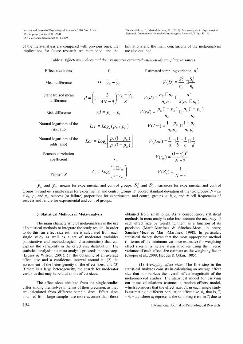
phi coefficient, etc.). Table 1 presents some of the usual
effect-size indices applied in meta-analysis together with
their estimated sampling variances, 2
iσ , as they are used in
the statistical analyses of a meta-analysis (cf. Borenstein,
Hedges, Higgins, & Rothstein, 2009; Cooper et al., 2009).
Once the effect-size index most appropriate to the characteristics of the studies has been selected, it is applied
to each single study and its sampling variance is also
calculated with the corresponding formulas (cf., e.g.,
Borenstein et al., 2009). When a meta-analysis includes
studies with different designs (e.g., correlational and two-
group designs), there are formulas to transform different
effect-size indices into each other. For example, it is
possible to transform correlation coefficients into d indices,
and vice versa; or odds ratios into d indices (Sánchez-Meca,
Marín-Martínez, & Chacón-Moscoso, 2003).
(5) Statistical analysis and interpretation. The dataset in a meta-analysis is composed of a matrix where
the rows are the studies and the columns are the moderator
variables, the effect-size index calculated in each study, and
its sampling variance. With these data it is possible to carry
out statistical analyses, which have the following three
main objectives: (1) to calculate an average effect size and
its confidence interval; (b) to assess the heterogeneity of the
effect sizes around the average, and (c) to search for
moderator variables that can explain the heterogeneity
(Sutton & Higgins, 2008). The main characteristic of meta-
analysis is that statistical methods are used for integrating the study results. More details about how to statistically
analyze a meta-analytic database are presented in the next
point of this article.
(6) Publication. Finally, the results of a meta-
analysis have to be published following the same structure as any other scientific paper: Introduction, method, results,
and discussion and conclusions (Botella & Gambara, 2006;
Rosenthal, 1995). A literature review on the topic is
outlined in the introduction, together with definitions of the
constructs and variables implied in the research question,
and the objectives and hypotheses of the meta-analysis. In
the method section the following should be included: the
selection criteria of the studies, the search strategy of the
studies, the coding process of the study characteristics, the
effect-size index calculated in the single studies, and the
statistical analyses that were carried out in the meta-
analytic integration. In the results section the characteristics
of the studies are presented, together with the effect-size
distribution, the mean effect size, the heterogeneity
assessment, and the results of the statistical analyses for
searching for moderator variables related to the effect sizes.
Finally, in the discussion and conclusion section the results
International Journal of Psychological Research, 2010. Vol. 3. No. 1. ISSN impresa (printed) 2011-2084 ISSN electrónica (electronic) 2011-2079
Sánchez-Meca, J., Marín-Martínez, F., (2010). Meta-analysis in Psychological Research. International Journal of Psychological Research, 3 (1), 151-163.
154 International Journal of Psychological Research
of the meta-analysis are compared with previous ones, the
implications for future research are mentioned, and the
limitations and the main conclusions of the meta-analysis
are also outlined.
Table 1. Effect-size indices and their respective estimated within-study sampling variances
Effect-size index Ti Estimated sampling variance, 2
iσ
Mean difference CE
yyD −=
C
C
E
E
n
S
n
SDV
22
)( +=
Standardized mean
difference S
yy
�d CE
−
−−=
94
31
)(2)(
2
CECE
CE
nn
d
nn
nndV
+++=
Risk difference CEpprd −=
C
CC
E
EE
n
pp
n
pprdV
)1()1()(
−+−=
Natural logarithm of the
risk ratio )/(
CEeppLogLrr =
CC
C
EE
E
pn
p
pn
pLrrV
−+−= 11)(
Natural logarithm of the
odds ratio)
−−=
)1(
)1(
EC
CE
e
pp
ppLogLor
dcbaLorV
1111)( +++=
Pearson correlation
coefficient
rxy 2
)1()(
22
−−
=�
rrV
xy
xy
Fisher’s Z
−+
=xy
xy
er
r
rLogZ
1
1
3
1)(
−=�
ZVr
Ey and
Cy : means for experimental and control groups.
2
ES and
2
CS : variances for experimental and control
groups. nE and nC: sample sizes for experimental and control groups. S: pooled standard deviation of the two groups. ' = nE
+ nC. pE and pC: success (or failure) proportions for experimental and control groups. a, b, c, and d: cell frequencies of success and failure for experimental and control groups.
3. Statistical Methods in Meta-analysis
The main characteristic of meta-analysis is the use
of statistical methods to integrate the study results. In order
to do this, an effect size estimate is calculated from each
single study as well as a set of moderator variables
(substantive and methodological characteristics) that can
explain the variability in the effect size distribution. The statistical analysis in a meta-analysis proceeds in three steps
(Lipsey & Wilson, 2001): (1) the obtaining of an average
effect size and a confidence interval around it; (2) the
assessment of the heterogeneity of the effect sizes, and (3)
if there is a large heterogeneity, the search for moderator
variables that may be related to the effect sizes.
The effect sizes obtained from the single studies
differ among themselves in terms of their precision, as they
are calculated from different sample sizes. Effect sizes
obtained from large samples are more accurate than those
obtained from small ones. As a consequence, statistical
methods in meta-analysis take into account the accuracy of
each effect size by weighting them as a function of its
precision (Marín-Martínez & Sánchez-Meca, in press;
Sánchez-Meca & Marín-Martínez, 1998). In particular,
statistical theory shows that the most appropriate method
(in terms of the minimum variance estimate) for weighting
effect sizes in a meta-analysis involves using the inverse variance of each effect size estimate as the weighting factor
(Cooper et al., 2009; Hedges & Olkin, 1985).
(1) Averaging effect sizes. The first step in the
statistical analyses consists in calculating an average effect
size that summarizes the overall effect magnitude of the meta-analyzed studies. The statistical model for carrying
out these calculations assumes a random-effects model,
which considers that the effect size, Ti, in each single study
is estimating a different population effect size, θi, that is, Ti
= θi + ui, where ui represents the sampling error in Ti due to

International Journal of Psychological Research, 2010. Vol. 3. No. 1.
ISSN impresa (printed) 2011-2084
ISSN electrónica (electronic) 2011-2079
Sánchez-Meca, J., Marín-Martínez, F., (2010). Meta-analysis in Psychological
Research. International Journal of Psychological Research, 3 (1), 151-163.
International Journal of Psychological Research 155
the fact that the single study is based on a random sample
selected from the population of potential participants (Field,
2003; Hedges & Vevea, 1998; Schmidt, Oh, & Hayes,
2009). The sampling error is quantified through the within-
study sampling variance, 2
iσ . Thus, it is assumed that in a
given meta-analysis the included studies constitute a
random sample of the studies which could have been
carried out about the same topic. Moreover, for the included
studies it is almost sure that the research conditions differ someway (e.g., in the therapist’s experience, the treatment’s
design and length, etc.), so it is reasonable to suspect that
the effect sizes could vary owing to these differences. Thus,
a distribution of population effect sizes, θi, with a mean
population effect size, µθ, is assumed, that is, θi = µθ + εi, with εi being the deviations of the population effect sizes
from its mean. The variability of the population effect sizes
is called the between-studies variance, τ2, or heterogeneity variance. Hence, in a random-effects model it is assumed
that each effect size estimate includes two variability
sources: the within-study variance, 2
iσ , and the between-
studies variance, τ2. The statistical model can be formulated
as:
Ti=µθ+εi+ui. (1)
When εi = 0, then the random-effects model
becomes a fixed-effects model, where there is only one
variability source, the within-study variance 2
iσ , and all of
the studies are estimating the same population effect size.
Thus, the statistical model is simplified to Ti = µθ + ui, and
µθ = θi.
In practice the meta-analyst will have to decide
which statistical model to apply, the fixed- or the random-
effects model. The consequences of assuming a random-
effects model or a fixed-effects one concern the
interpretation of the results and also the results obtained
themselves. On the one hand, a meta-analyst that applies a
fixed-effects model is assuming that his/her results can only
be generalized to an identical population of studies to that
of the individual studies included in the meta-analysis,
whereas in a random-effects model the results can be
generalized to a wider population of studies. On the other
hand, the error attributed to the effect size estimates in a
fixed-effects model is smaller than in a random-effects
model, which is why in the first model the confidence
intervals are narrower and the statistical tests more liberal than in the second one. The main consequence of assuming
a fixed-effects model when the meta-analytic data come
from a random-effects model is that we may attribute more
precision to the effect size estimates than is really
appropriate and that we may find statistically significant relationships between variables that are actually spurious.
Consequently, it is more realistic to assume random-effects
models in meta-analysis.
In order to apply statistical inference, it is usually assumed that the effect size distribution, Ti, in a random-
effects model follows a normal distribution with population
mean µθ and variance equal to the sum of the two
variability sources, 2
iσ + τ2, that is, Ti ∼ '(µθ;
2
iσ + τ2).
Thus, the uniformly minimum variance unbiased
estimator of µθ, UT , is given by (Viechtbauer, 2005):
∑
∑=
i
i
i
ii
w
Tw
T U , (2)
where wi are the optimal weights, defined as
( )22
iiτσ1 +=w . The variance of UT is given by:
∑=
i
iw
TV1
)( U . (3)
However, in practice the optimal weights cannot
be calculated, because the parametric within-study
variances, 2
iσ , and the parametric between-studies
variance, τ2, are unknown. Therefore, the two kinds of
variance have to be estimated from the data. In general, good estimators of the within-study variance for the
different effect-size indices have been proposed in the
meta-analytic literature (cf. e.g., Borenstein et al., 2009).
About a dozen different estimators have been proposed for
estimating the between-studies variance (Sánchez-Meca &
Marín-Martínez, 2008; Viechtbauer, 2005). Of these, the
most usually applied are those based on the moments
method, 2
DLτ , proposed by DerSimonian and Laird (1986),
and the one based on restricted maximum likelihood, 2
REMLτ (Thompson & Sharp, 1999). The moments method
estimator is given by:
c
kQ )1(τ2DL
−−= , (4)
where k is the number of studies in the meta-
analysis; Q is the heterogeneity statistic defined as:
( )∑ −=i
iiTTwQ
2~
~ , (5)

International Journal of Psychological Research, 2010. Vol. 3. No. 1.
ISSN impresa (printed) 2011-2084
ISSN electrónica (electronic) 2011-2079
Sánchez-Meca, J., Marín-Martínez, F., (2010). Meta-analysis in Psychological
Research. International Journal of Psychological Research, 3 (1), 151-163.
156 International Journal of Psychological Research
with 2
iiσ1
~ =w being the estimated weights by
assuming a fixed-effects model, and T~
being the average
effect size also by assuming a fixed-effects model, that is:
∑∑=i
i
i
iiwTwT~~
~
. Finally, in equation (4), c is
obtained by:
∑∑
∑−=
i
i
i
i
i
i
w
w
wc ~
)~(~
2
. (6)
In Equation (4), when Q < (k – 1), then 2
DLτ is
truncated to 0 to avoid negative values.
The between-studies variance estimator
based on restricted maximum likelihood, 2
REMLτ , is
obtained by iterating until convergence the equation
(Thompson & Sharp, 1999):
( )[ ]∑∑
∑+
−−=
i
i
i
i
i
ii
ww
TTw
22
2
i
2
REML2
2
REMLˆ
1
ˆ
σˆ
τ (7)
with )τσ(1ˆ 22
ii+=w , where
2τ is initially 0 or
it is estimated by any of the noniterative estimators of the
between-studies variance (e.g., 2
DLτ ) and REMLT is given
by:
∑
∑=
i
i
i
ii
w
Tw
Tˆ
ˆ
REML . (8)
In each iteration of Equations (7) and (8), each
estimate of τ2 must be checked in order to avoid negative values.
Once we have an estimate of the between-studies
variance (2
DLτ or
2
REMLτ ) and the effect estimates, Ti, and
their estimated within-study variances, 2
iσ , it is possible to
calculate an average effect size by:
∑
∑=
i
i
i
ii
w
Tw
Tˆ
ˆ
, (9) with
)τσ(1ˆ 22
ii+=w . Then a confidence interval for T is
usually calculated by assuming a normal distribution:
)(2/
TVzT α± , (10)
where zα/2 is the 100(α/2) percentile of the standard normal
distribution, α being the significance level; and )(TV is
the sampling variance of the average effect size, which is
obtained by:
∑=
i
iw
TVˆ
1)( . (11)
Although Equation (10) is the usual procedure for
calculating a confidence interval around the overall effect
size, this method does not take into account the uncertainty
produced by the fact that the within-study and the between-
studies variances have to be estimated. As a consequence,
the confidence interval will underestimate the nominal
confidence level. A confidence interval that better fits the
nominal confidence level is that proposed by Hartung (1999; see also Sánchez-Meca & Marín-Martínez, 2008;
Sidik & Jonkman, 2003, 2006), which assumes a Student t-
distribution with k – 1 degrees of freedom and estimates the
sampling variance of the overall effect size by an improved
formula:
)(W2/,1TVtT
k α−± , (12)
where )(WTV is the improved sampling variance estimate
and is given by:
( )∑
∑
−
−=
i
i
i
ii
wk
TTw
TVˆ)1(
ˆ
)(
2
W. (13)
Finally, together with the average effect size and
its confidence interval, it is very informative to present a
graph that was specially developed for meta-analysis named
‘forest plot’. A forest plot is a graphical presentation of
each effect size estimate with its confidence interval and the
overall effect size also with its confidence interval. Thus, a
forest plot is something like a photograph of the effect
estimates obtained in the meta-analysis (Borenstein et al.,
2009; Higgins & Green, 2008).
(2) Assessing heterogeneity. Whilst it is important
in meta-analysis to obtain an overall effect size, it is even
more important to assess the heterogeneity of the effect
estimates around its mean. We need to know whether the
variability in the effect sizes is due only to sampling error
or if there is more variability than can be explained by
sampling error. This question is usually answered by

International Journal of Psychological Research, 2010. Vol. 3. No. 1.
ISSN impresa (printed) 2011-2084
ISSN electrónica (electronic) 2011-2079
Sánchez-Meca, J., Marín-Martínez, F., (2010). Meta-analysis in Psychological
Research. International Journal of Psychological Research, 3 (1), 151-163.
International Journal of Psychological Research 157
applying the heterogeneity Q statistic, which was defined in
Equation (5). Under the null hypothesis of heterogeneity
due only to sampling error, the Q statistic follows a Chi-
square distribution with k – 1 degrees of freedom. Thus, by
comparing Q with the 100(1 – α) percentile of 2
1−kχ
distribution, it is possible to make a statistical decision
about this question.
When a meta-analysis has a small number of
studies, the Q statistic has low statistical power (Harwell,
1997; Sánchez-Meca & Marín-Martínez, 1997). Thus, it is
usual to assess heterogeneity by complementing the Q statistic with the I
2 index, a percentage that informs us
about the extent of variability in the effect size distribution
due to true heterogeneity (that is, heterogeneity not due to
sampling error, but to the influence of many different
moderator variables). The I2 index is calculated by (Higgins
& Thompson, 2002):
100)1(2 ×−−=
Q
kQI . (14)
When Q < (k – 1) then I2 is truncated to 0. Higgins
and Thompson (2002) proposed a tentative classification of I2 by stating that I
2 values around 25%, 50%, and 75% can
be considered as reflecting small, medium, and large
heterogeneity, respectively.
(3) Searching for moderator variables. When the
Q statistic achieves a statistically significant result and the I2 index is of medium to large magnitude, then the overall
effect size calculated in the first step of the statistical
analyses does not adequately represent all of the study
results. As a consequence, the next step in the analyses
consists in searching for moderator variables that can explain the heterogeneity. In this phase of the analysis, the
effect estimates, Ti, act as the dependent variable, whereas
the moderator variables are potential predictors that may be
related to the effect estimates. Depending on the categorical
or continuous nature of the moderator variables, analyses of
variance (ANOVAs) or regression analyses are applied in order to examine the influence of these predictors on the
effect magnitude. In all cases, however, weighting methods
are applied that take into account the precision of the effect
estimates. In particular, the most appropriate statistical
model for testing the influence of moderator variables in
meta-analysis is to assume a mixed-effects model, where
the moderator variable is the fixed-effects component and
the studies are the random-effects component in the model
(Konstantopoulos & Hedges, 2009; Raudenbush, 2009).
For categorical moderator variables, ANOVAs are
applied by weighted least squares estimation. An ANOVA
for testing the significance of a categorical moderator
variable with m categories consists of calculating a
weighted average effect size for each category, jT , and
obtaining the QB statistic by:
( )∑ −=m
j
TTwQ2
jjBˆ , (15)
with )(1ˆ jj TVw = , and ∑=jm
i
wTV ijj ˆ1)( . The QB
statistic is the weighted between-categories sum of squares
of the ANOVA. Under the null hypothesis of no difference
between the mean effect sizes for the m categories
(m1
θθ0µ...µ: ==H ), the QB statistic follows a Chi-
square distribution with m – 1 degrees of freedom. Thus,
from comparing the QB statistic with the 100(1 – α)
percentile of 2
1−mχ distribution, it is possible to decide
whether the moderator variable is statistically related to the
effect size.
The result of QB is complemented with a
misspecification test that can be applied separately for each
category of the moderator variable. Thus, the jWQ statistic
for the jth category is obtained by:
( )∑ −=jm
i
TTwQ2
jijijWˆ
j. (16)
A different jWQ statistic is calculated for each
category of the moderator variable in order to examine the
heterogeneity of the effect sizes within a given category.
Thus, under the null hypothesis of homogeneous effect
sizes in the jth category, the jWQ statistic follows a Chi-
square distribution with mj – 1 degrees of freedom, where
mj is the number of effect sizes in the jth category.
Therefore, by comparing jWQ with the 100(1 – α)
percentile of 2
1−jmχ distribution, it is possible to decide
whether the effect sizes in the jth category are
homogeneous. In addition, a global misspecification test for
all ANOVA model consists of calculating the sum of the m
jWQ statistics as follows:
m1WW
... QQQW
++= . (17)
The QW statistic is the weighted within-categories sum of squares of the ANOVA. Thus, under the null
hypothesis of global homogeneity for all categories, the QW
statistic follows a Chi-square distribution with k – m

International Journal of Psychological Research, 2010. Vol. 3. No. 1.
ISSN impresa (printed) 2011-2084
ISSN electrónica (electronic) 2011-2079
Sánchez-Meca, J., Marín-Martínez, F., (2010). Meta-analysis in Psychological
Research. International Journal of Psychological Research, 3 (1), 151-163.
158 International Journal of Psychological Research
degrees of freedom. By comparing QW with the 100(1 – α)
percentile of 2
mk−χ distribution, it is possible to decide
whether the ANOVA model is globally misspecified.
When the moderator variable is continuous or we
are interested in examining the influence of a set of
moderator variables (continuous and/or categorical), weighted simple or multiple linear regression models can
be applied. By assuming a mixed-effects model, where the
moderator variables are the fixed-effects component and the
studies the random-effects component, the linear model is
given by:
εuXβT ++= , (18)
with T being a k by 1 vector of effect size
estimates with elements {Ti}, X is a k by P matrix of
predictors, with P = p + 1 columns (p being the number of
predictors), β is a P by 1 vector of parametric regression
coefficients with elements {βj}, u is a k by 1 vector of
within-study estimation errors with elements {ui}, and ε is a
scalar with the between-studies variance {ε}. T has
variance V(u + ε) = τ2I + V, with I being a k by k identity matrix and V being a k by k diagonal matrix with elements
{22
iiτσ +=v }.
The vector of regression coefficients, β, is
estimated by:
WTX'WX)X'β-1
(ˆ = , (19)
with 1ˆ −= VW , W being a k by k diagonal matrix with the
weights for each effect size, {iw }, which are estimated by
the inverse of the sum of the within-study and the between-
studies variances: )τσ(1ˆ 22
ii+=w . In this case, the
between-studies variance is estimated by an extension of
Equations (4) or (7) to the case of a regression model with p
predictors. For example, an extension of the moments method estimator is given by:
[ ]WX'WXX'WXW1
2
MM
)()(
)1(τ −−
−−−=trtr
pkQE , (20)
where QE is the weighted residual sum of squares of the model and is obtained by:
REQQ -WTT'= . (21)
The between-studies variance estimator based on
restricted maximum likelihood for a weighted regression
model can be consulted in Thompson and Sharp (1999).
A test for the statistical significance of the
full model is given by the QR statistic, which is the
weighted regression sum of squares and is given by:
βS'β-1 ˆˆˆR β=Q , (22)
where βS is the matrix of variances and covariances for
the regression coefficients. Under the null hypothesis of no
relationship between the composite of predictors and the
effect sizes (H0: β = 0), QR follows a Chi-square
distribution with P degrees of freedom. By comparing QR
with the 100(1 – α) percentile of 2
Pχ distribution, it is
possible to decide if the full model shows a statistically significant relationship with the effect size. At the same
time, statistical tests for individual predictors can also be
applied in order to examine the influence of each predictor
once that of the other predictors in the model has been
partialized. For a given regression coefficient, jβ , the null
hypothesis of no effect is tested by:
)ˆ(
ˆZ
j
j
βV
β= , (23)
with )ˆ( jβV being the jth diagonal element of the
P by P matrix for the variances and covariances of the
regression coefficients. Thus, comparing |Z| with the 100(1
– α/2) percentile of the standard normal distribution, it is
possible to determine the statistical significance of a given
predictor in the multiple regression model.
Finally, a specification test of the regression model
is applied by means of the QE statistic defined in Equation
(21). Under the null hypothesis that the model is well
specified (H0: 0τ2
WLS= ), QE follows a Chi-square
distribution with k – p –1 degrees of freedom. Thus, by
comparing QE with the 100(1 – α) percentile of 2
1−−pkχ
distribution, it is possible to examine the model
misspecification.
4. An Illustrative Example
In order to illustrate the calculations in a typical
meta-analysis, Table 2 presents some of the data obtained
in a meta-analysis on the efficacy of psychological
treatments for obsessive-compulsive disorder (OCD; Rosa-
Alcázar et al., 2008). This meta-analysis is composed of 24
studies that compared two groups of patients with OCD,
one receiving a psychological treatment (experimental
International Journal of Psychological Research, 2010. Vol. 3. No. 1.
ISSN impresa (printed) 2011-2084
ISSN electrónica (electronic) 2011-2079
Sánchez-Meca, J., Marín-Martínez, F., (2010). Meta-analysis in Psychological
Research. International Journal of Psychological Research, 3 (1), 151-163.
International Journal of Psychological Research 159
group) and the other one not receiving treatment (control
group). The effect-size index calculated in each study was
the standardized mean difference, d, defined as the
difference between the means for the treatment and control groups divided by a pooled estimate of the standard
deviations for the two groups. Positive values for d
indicated a lower level of obsessions and compulsions after
treatment in the treated group in comparison with the
control group, whereas negative values for d indicated a
higher level. Table 2 also includes the sample sizes for the
two groups (nE and nC), as well as the estimated within-
study sampling variance for each effect size (2
iσ ).
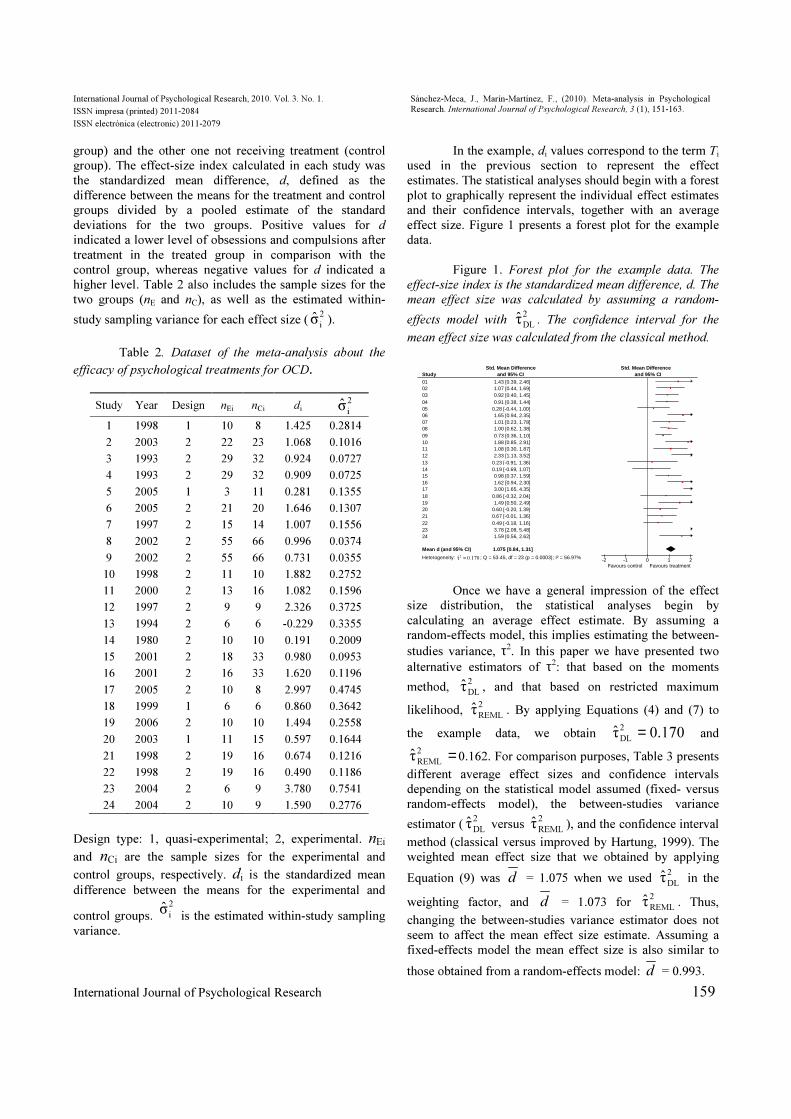
Table 2. Dataset of the meta-analysis about the
efficacy of psychological treatments for OCD.
Study Year Design nEi nCi di 2
iσ
1 1998 1 10 8 1.425 0.2814
2 2003 2 22 23 1.068 0.1016
3 1993 2 29 32 0.924 0.0727
4 1993 2 29 32 0.909 0.0725
5 2005 1 3 11 0.281 0.1355
6 2005 2 21 20 1.646 0.1307
7 1997 2 15 14 1.007 0.1556
8 2002 2 55 66 0.996 0.0374
9 2002 2 55 66 0.731 0.0355
10 1998 2 11 10 1.882 0.2752
11 2000 2 13 16 1.082 0.1596
12 1997 2 9 9 2.326 0.3725
13 1994 2 6 6 -0.229 0.3355
14 1980 2 10 10 0.191 0.2009
15 2001 2 18 33 0.980 0.0953
16 2001 2 16 33 1.620 0.1196
17 2005 2 10 8 2.997 0.4745
18 1999 1 6 6 0.860 0.3642
19 2006 2 10 10 1.494 0.2558
20 2003 1 11 15 0.597 0.1644
21 1998 2 19 16 0.674 0.1216
22 1998 2 19 16 0.490 0.1186
23 2004 2 6 9 3.780 0.7541
24 2004 2 10 9 1.590 0.2776
Design type: 1, quasi-experimental; 2, experimental. nEi
and nCi are the sample sizes for the experimental and
control groups, respectively. di is the standardized mean
difference between the means for the experimental and
control groups. 2
iσ
is the estimated within-study sampling
variance.
In the example, di values correspond to the term Ti
used in the previous section to represent the effect
estimates. The statistical analyses should begin with a forest
plot to graphically represent the individual effect estimates and their confidence intervals, together with an average
effect size. Figure 1 presents a forest plot for the example
data.
Figure 1. Forest plot for the example data. The
effect-size index is the standardized mean difference, d. The
mean effect size was calculated by assuming a random-
effects model with 2
DLτ . The confidence interval for the
mean effect size was calculated from the classical method.
Once we have a general impression of the effect
size distribution, the statistical analyses begin by
calculating an average effect estimate. By assuming a random-effects model, this implies estimating the between-
studies variance, τ2. In this paper we have presented two
alternative estimators of τ2: that based on the moments
method, 2
DLτ , and that based on restricted maximum
likelihood, 2
REMLτ . By applying Equations (4) and (7) to
the example data, we obtain 170.0τ2
DL= and
=2
REMLτ 0.162. For comparison purposes, Table 3 presents
different average effect sizes and confidence intervals
depending on the statistical model assumed (fixed- versus
random-effects model), the between-studies variance
estimator (2
DLτ versus
2
REMLτ ), and the confidence interval
method (classical versus improved by Hartung, 1999). The
weighted mean effect size that we obtained by applying
Equation (9) was d = 1.075 when we used 2
DLτ in the
weighting factor, and d = 1.073 for 2
REMLτ . Thus,
changing the between-studies variance estimator does not
seem to affect the mean effect size estimate. Assuming a
fixed-effects model the mean effect size is also similar to
those obtained from a random-effects model: d = 0.993.
Study 01 02 03 04 05 06 07 08 09 10 11 12 13 14 15 16 17 18 19 20 21 22 23 24
Mean d (and 95% CI)
Heterogeneity: 170.0τ2 = ; Q = 53.45, df = 23 (p = 0.0003); I² = 56.97%
and 95% CI 1.43 [0.39, 2.46] 1.07 [0.44, 1.69] 0.92 [0.40, 1.45] 0.91 [0.38, 1.44]
0.28 [-0.44, 1.00] 1.65 [0.94, 2.35] 1.01 [0.23, 1.78] 1.00 [0.62, 1.38] 0.73 [0.36, 1.10] 1.88 [0.85, 2.91] 1.08 [0.30, 1.87] 2.33 [1.13, 3.52]
0.23 [-0.91, 1.36] 0.19 [-0.69, 1.07] 0.98 [0.37, 1.59] 1.62 [0.94, 2.30] 3.00 [1.65, 4.35]
0.86 [-0.32, 2.04] 1.49 [0.50, 2.49]
0.60 [-0.20, 1.39] 0.67 [-0.01, 1.36] 0.49 [-0.18, 1.16] 3.78 [2.08, 5.48] 1.59 [0.56, 2.62]
1.075 [0.84, 1.31]
Std. Mean Difference Std. Mean Difference and 95% CI
-2 -1 0 1 2 Favours control Favours treatment

International Journal of Psychological Research, 2010. Vol. 3. No. 1.
ISSN impresa (printed) 2011-2084
ISSN electrónica (electronic) 2011-2079
Sánchez-Meca, J., Marín-Martínez, F., (2010). Meta-analysis in Psychological
Research. International Journal of Psychological Research, 3 (1), 151-163.
160 International Journal of Psychological Research
Table 3. Summary statistics for the average effect size and its confidence interval calculated from different methods
Statistical model τ2 estimator CI method d 95% C. I.
dl du
Width
of the CI
RE model 170.0τ2
DL= Classical 1.075 0.843 1.306 0.463
RE model 170.0τ2
DL= Improved 1.075 0.786 1.363 0.577
RE model 162.0τ2
REML= Classical 1.073 0.844 1.302 0.458
RE model 162.0τ2
REML= Improved 1.073 0.785 1.360 0.572
FE model -- Classical 0.993 0.852 1.134 0.282
RE: random-effects model. FE: fixed-effects model. CI: confidence interval. d : average effect size. dl and du:
lower and upper confidence limits for the average effect size.
Following Cohen’s (1988) benchmarks for
interpreting the practical significance of an effect size, we can consider that d values around 0.20, 0.50, and 0.80 can
be interpreted as reflecting an effect of small, medium, and
large magnitude, respectively. Therefore, a mean effect size
in our example of d = 1.075 can be interpreted as
indicating a high effect of psychological treatments in
reducing obsessions and compulsions of patients with
OCD.
Table 3 also shows confidence intervals for the
average effect size depending on the method selected
(classical versus improved by Hartung, 1999) and on the
between-studies variance estimator (moments method
versus restricted maximum likelihood). With the classical
method for calculating a confidence interval around the
mean effect size the width of the confidence interval (0.463
and 0.458 for 2
DLτ and
2
REMLτ , respectively) was smaller
than that of the improved method (0.577 and 0.572 for 2
DLτ
and 2
REMLτ ). The classical method is, therefore, slightly
more liberal in comparison with the improved method. The
most liberal method, however, is the confidence interval
which assumes a fixed-effects model as it does not take into
account the between-studies variability among the effect
sizes.
Once we have an estimate of the overall effect
magnitude in the meta-analysis, the next step in the
analyses consists of assessing the heterogeneity of the
effect sizes. By applying Equation (5) to our example data,
we obtained Q(23) = 53.452, p = .0003, which enabled us
to reject the null hypothesis of homogenous effect sizes.
The statistically significant result for the Q statistic is complemented with the calculation of the I
2 index by
Equation (14), reaching a moderate heterogeneity, I2 =
56.97%. Therefore, we can conclude that the effect sizes
were clearly heterogeneous and, as a consequence, the next
step in the analyses is to search for moderator variables which are able to explain the effect size variability.
In order to illustrate how to test different moderator variables on the effect sizes, here we have
selected two of them: one categorical variable and the other
continuous. As an example of a categorical moderator
variable, we have selected the design type, distinguishing
between experimental (random assignment to the groups)
versus quasi-experimental designs (nonrandom
assignment). For comparison purposes, Table 4 shows the
weighted ANOVA results for the design type by assuming a
mixed-effects model with two different estimators of the
between-studies variance (2
MMτ and
2
REMLτ ) and a fixed-
effects model. In the three cases we obtained, using
Equation (15), a nonstatistically significant result for the QB
statistic, leading to the conclusion that the type of design
does not seem to affect the effect sizes, although quasi-
experimental designs presented a mean effect size thatwas
slightly lower than that of the experimental ones. Wecan
also observe how the QB statistic for the fixed-effects model was the most liberal of the three models applied.
Table 4. Results of the weighted A'OVA applied
on the design type by assuming a random-effects model
with 2
MMτ and
2
REMLτ , and for a fixed-effects model.
Mixed-Effects Model with 168.0τ2
MM=
Design type k jd
95% C. I.
dl du QWj
D
F p
Quasi-exptal
Exptal
4
20
0.721
1.134
0.114 1.329
0.884 1.384
1.822
29.069
3
19
.610
.065
ANOVA results
QB(1) = 1.514, p = .218 QW(22) = 30.891, p = .098
Mixed-Effects Model with 113.0τ2
REML=
Design type
k jd 95% C. I. dl du
QWj DF
p
Quasi-exptal
Exptal
4
20
0.710
1.114
0.149 1.270
0.889 1.339
2.127
32.864
3
19
.546
.025
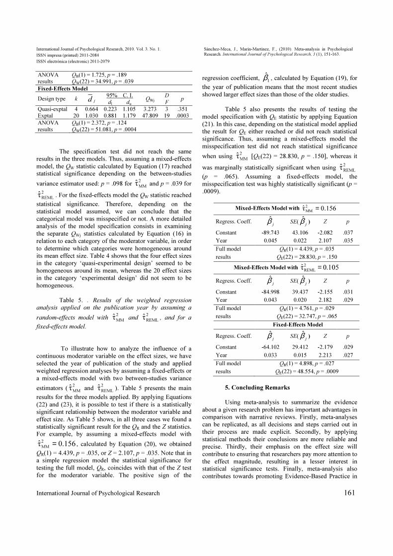
International Journal of Psychological Research, 2010. Vol. 3. No. 1.
ISSN impresa (printed) 2011-2084
ISSN electrónica (electronic) 2011-2079
Sánchez-Meca, J., Marín-Martínez, F., (2010). Meta-analysis in Psychological
Research. International Journal of Psychological Research, 3 (1), 151-163.
International Journal of Psychological Research 161
ANOVA results
QB(1) = 1.725, p = .189 QW(22) = 34.991, p = .039
Fixed-Effects Model
Design type k jd 95% C. I.
dl du QWj
D
F p
Quasi-exptal Exptal
4 20
0.664 1.030
0.223 1.105 0.881 1.179
3.273 47.809
3 19
.351 .0003
ANOVA
results
QB(1) = 2.372, p = .124
QW(22) = 51.081, p = .0004
The specification test did not reach the same
results in the three models. Thus, assuming a mixed-effects
model, the QW statistic calculated by Equation (17) reached statistical significance depending on the between-studies
variance estimator used: p = .098 for 2
MMτ and p = .039 for
2
REMLτ . For the fixed-effects model the QW statistic reached
statistical significance. Therefore, depending on the
statistical model assumed, we can conclude that the
categorical model was misspecified or not. A more detailed
analysis of the model specification consists in examining
the separate QWj statistics calculated by Equation (16) in
relation to each category of the moderator variable, in order
to determine which categories were homogeneous around
its mean effect size. Table 4 shows that the four effect sizes in the category ‘quasi-experimental design’ seemed to be
homogeneous around its mean, whereas the 20 effect sizes
in the category ‘experimental design’ did not seem to be
homogeneous.
Table 5. . Results of the weighted regression
analysis applied on the publication year by assuming a
random-effects model with 2
MMτ and
2
REMLτ , and for a
fixed-effects model.
To illustrate how to analyze the influence of a
continuous moderator variable on the effect sizes, we have
selected the year of publication of the study and applied
weighted regression analyses by assuming a fixed-effects or
a mixed-effects model with two between-studies variance
estimators (2
MMτ and
2
REMLτ ). Table 5 presents the main
results for the three models applied. By applying Equations
(22) and (23), it is possible to test if there is a statistically
significant relationship between the moderator variable and
effect size. As Table 5 shows, in all three cases we found a
statistically significant result for the QR and the Z statistics. For example, by assuming a mixed-effects model with
156.0τ2
MM= , calculated by Equation (20), we obtained
QR(1) = 4.439, p = .035, or Z = 2.107, p = .035. Note that in
a simple regression model the statistical significance for
testing the full model, QR, coincides with that of the Z test
for the moderator variable. The positive sign of the
regression coefficient, 1
β , calculated by Equation (19), for
the year of publication means that the most recent studies
showed larger effect sizes than those of the older studies.
Table 5 also presents the results of testing the
model specification with QE statistic by applying Equation
(21). In this case, depending on the statistical model applied the result for QE either reached or did not reach statistical
significance. Thus, assuming a mixed-effects model the
misspecification test did not reach statistical significance
when using 2
MMτ [QE(22) = 28.830, p = .150], whereas it
was marginally statistically significant when using 2
REMLτ
(p = .065). Assuming a fixed-effects model, the
misspecification test was highly statistically significant (p =
.0009).
5. Concluding Remarks
Using meta-analysis to summarize the evidence
about a given research problem has important advantages in
comparison with narrative reviews. Firstly, meta-analyses
can be replicated, as all decisions and steps carried out in
their process are made explicit. Secondly, by applying
statistical methods their conclusions are more reliable and
precise. Thirdly, their emphasis on the effect size will
contribute to ensuring that researchers pay more attention to
the effect magnitude, resulting in a lesser interest in statistical significance tests. Finally, meta-analysis also
contributes towards promoting Evidence-Based Practice in
Mixed-Effects Model with 156.0τ2
MM=
Regress. Coeff. j
β SE(j
β ) Z p
Constant
Year
-89.743
0.045
43.106
0.022
-2.082
2.107
.037
.035
Full model
results
QR(1) = 4.439, p = .035
QE(22) = 28.830, p = .150
Mixed-Effects Model with 105.0τ2
REML=
Regress. Coeff. j
β SE(j
β ) Z p
Constant
Year
-84.998
0.043
39.437
0.020
-2.155
2.182
.031
.029
Full model
results
QR(1) = 4.761, p = .029
QE(22) = 32.747, p = .065
Fixed-Effects Model
Regress. Coeff. j
β SE(j
β ) Z p
Constant
Year
-64.102
0.033
29.412
0.015
-2.179
2.213
.029
.027
Full model
results
QR(1) = 4.898, p = .027
QE(22) = 48.554, p = .0009
International Journal of Psychological Research, 2010. Vol. 3. No. 1.
ISSN impresa (printed) 2011-2084
ISSN electrónica (electronic) 2011-2079
Sánchez-Meca, J., Marín-Martínez, F., (2010). Meta-analysis in Psychological
Research. International Journal of Psychological Research, 3 (1), 151-163.
162 International Journal of Psychological Research
Psychology, a new methodological approach that aims to
encourage professionals to base their practice to the greatest
extent possible on scientific evidence obtained from
research.
Nevertheless meta-analysis has problems and
limitations. On the one hand, the validity and accuracy of
the results in a meta-analysis depend on the quality of the
empirical studies integrated. If the single studies offer
biased estimations of the effects, then the meta-analytic
results will also be biased. An assessment of the
methodological quality of the single studies is therefore one
of the main requisites in any meta-analysis (cf. e.g.,
Valentine & Cooper, 2008). In addition, meta-analysis can
suffer publication bias if it is only based on published studies. As a consequence, an analysis of publication bias is
essential in any meta-analysis (Rothstein, Sutton, &
Borenstein, 2005). Moreover, meta-analysis can suffer
selection bias, when the selection criteria for including
single studies in the meta-analysis are affected by
theoretical or substantive preferences of the meta-analyst. A
reliability analysis of the selection process of the studies
should be therefore accomplished in order to avoid bias in
this step of the meta-analysis. Finally, meta-analyses can be
affected by reporting bias when the single studies only
reported statistical data on the outcomes with positive
results for the hypothesis tested. A detailed analysis of the
design and the dependent variables included in the single
studies should be carried out to assess whether studies are
selectively reporting their statistical results.
As meta-analyses can suffer deficiencies and
biases in their development and in their reporting practices,
they should be read critically. To this end, several protocols
and statements have been published that enable consumers
of meta-analyses to assess their methodological quality. It is
worth noting the recent publication of the PRISMA
checklist (‘Preferred Reported Items for Systematic reviews and Meta-Analyses; Moher, Liberati, Tetzlaff et al., 2009),
a set of guidelines to assess the methodological quality in
reporting practices of meta-analyses. Another endeavor
along the same lines is the publication of the AMSTAR
protocol for critical appraisal of meta-analyses (Shea,
Grimshaw, Wells et al., 2007).
Finally, several software programs have been
developed for carrying out statistical analyses in meta-
analysis. David B. Wilson has developed macros for doing
meta-analysis in SPSS, SAS, and STATA. The macros can be freely obtained from the web site
http://mason.gmu.edu/~dwilsonb/ma.html. The Cochrane
Collaboration has developed RevMan 5.0.22, another free
program for carrying out meta-analysis that can be obtained
from the web site of this Collaboration
(www.cochrane.org). Finally, there is a commercial program Comprehensive Meta-analysis 2.0 (Borenstein,
Hedges, Higgins, & Rothstein, 2005; www.meta-
analysis.com).
REFERE�CES
Borenstein, M. J., Hedges, L. V., Higgins, J. P. T., &
Rothstein, H. (2005). Comprehensive Meta-
analysis (Vers.2). Englewood Cliffs, NJ: Biostat,
Inc.
Borenstein, M. J., Hedges, L. V., Higgins, J. P. T., &
Rothstein, H. R. (2009). Introduction to meta-
analysis. Chichester, UK: Wiley. Botella, J., & Gambara, H. (2006). Doing and reporting a
meta-analysis. International Journal of Clinical
and Health Psychology, 6, 425-440.
Cohen, J. (1988). Statistical power analysis for the
behavioral sciences (2nd ed.). Hillsdale, NJ:
Erlbaum.
Cook, T. D., Cooper, H., Cordray, D. S., Hartmann, H.,
Hedges, L. V., Light, R. J., Louis, T. A., &
Mosteller, F. (1992). Meta-analysis for
explanation: A casebook. New York: Russell Sage
Foundation.
Cooper, H. (2010). Research synthesis and meta-analysis:
A step-by-step approach (3rd ed.). Thousand Oaks,
CA: Sage.
Cooper, H., Hedges, L. V., & Valentine, J. C. (Eds.)(2009).
The handbook of research synthesis and meta-
analysis (2nd ed.). New York: Russell Sage
Foundation.
DerSimonian, R., & Laird, N. (1986). Meta-analysis of
clinical trials. Controlled Clinical Trials, 7, 177-
188.
Egger, M., Davey Smith, G., & Altman, D. G. (Eds.)
(2001). Systematic reviews in health care: Meta-
analysis in context (2nd ed.). London: BMJ Pub.
Group.
Field, A. P. (2003). The problems of using fixed-effects
models of meta-analysis on real-world data.
Understanding Statistics, 2, 77-96.
Hartung, J. (1999). An alternative method for meta-analysis. Biometrical Journal, 41, 901-916.
Harwell, M. (1997). An empirical study of Hedges's
homogeneity test. Psychological Methods, 2, 219-
231.
Hedges, L. V., & Olkin, I. (1985). Statistical methods for
meta-analysis. New York: Academic Press.
Hedges, L. V., & Vevea, J. L. (1998). Fixed- and random-
effects models in meta-analysis. Psychological
Methods, 3, 486-504.
Higgins, J. P. T., & Green, S. (Eds.)(2008). Cochrane
handbook for systematic reviews of interventions. Chichester, UK: Wiley-Blackwell.

International Journal of Psychological Research, 2010. Vol. 3. No. 1.
ISSN impresa (printed) 2011-2084
ISSN electrónica (electronic) 2011-2079
Sánchez-Meca, J., Marín-Martínez, F., (2010). Meta-analysis in Psychological
Research. International Journal of Psychological Research, 3 (1), 151-163.
International Journal of Psychological Research 163
Higgins, J. P. T., & Thompson, S. G. (2002). Quantifying
heterogeneity in a meta-analysis. Statistics in
Medicine, 21, 1539-1558.
Hunter, J. E., & Schmidt, F. L. (2004). Methods of meta-
analysis: Correcting error and bias in research
synthesis (2nd ed.). Sage.
Konstantopoulos, S., & Hedges, L. V. (2009). Fixed effects
models. In H. Cooper, L. V. Hedges, & J. C.
Valentine (Eds.), The handbook of research
synthesis and meta-analysis (2nd ed.) (pp. 279-
293). New York: Russell Sage Foundation.
Lipsey, M. W., & Wilson, D. B. (2001). Practical Meta-
analysis. Thousand Oaks, CA: Sage
Littell, J. H., Corcoran, J., & Pillai, V. (2008). Systematic
reviews and meta-analysis. Oxford, UK: Oxford University Press.
Marín-Martínez, F., & Sánchez-Meca, J. (2010). Weighting
by inverse variance or by sample size in random-
effects meta-analysis. Educational and
Psychological Measurement, 70, 56-73.
Moher, D., Liberatti, A., Tetzlaff, J., Altman D. G., and the
PRISMA Group (2009). Preferred Reporting Items
for Systematic reviews and Meta-Analyses: The
PRISMA statement. PLOS Medicine, 6(7):
e1000097. doi:10.1371journal.pmed.1000097.
Petticrew, M., & Roberts, H. (2006). Systematic reviews in
the social sciences: A practical guide. Malden,
MA: Blackwell.
Raudenbush, S. W. (2009). Random effects models. In H.
Cooper, L. V. Hedges, & J. C. Valentine (Eds.),
The handbook of research synthesis and meta-
analysis (2nd ed.) (pp. 295-315). New York:
Russell Sage Foundation.
Rosa-Alcázar, A. I., Sánchez-Meca, J., Gómez-Conesa, A.,
& Marín-Martínez, F. (2008). Psychological
treatment of obsessive-compulsive disorder: A
meta-analysis. Clinical Psychology Review, 28,
1310-1325. Rosenthal, R. (1995). Writing meta-analytic reviews.
Psychological Bulletin, 118, 183-192.
Rothstein, H. R., Sutton, A. J., & Borenstein, M. (Eds.)
(2005). Publication bias in meta-analysis:
Prevention, assessment, and adjustments.
Chichester, UK: Wiley. Sánchez-Meca, J., & Marín-Martínez, F. (1997).
Homogeneity tests in meta-analysis: A Monte
Carlo comparison of statistical power and Type I
error. Quality and Quantity, 31, 385-399.
Sánchez-Meca, J., & Marín-Martínez, F. (1998). Weighting by inverse-variance or by sample size in meta-
analysis: A simulation study. Educational and
Psychological Measurement, 58, 211-220.
Sánchez-Meca, J., & Marín-Martínez, F. (2008).
Confidence intervals for the overall effect size in
random-effects meta-analysis. Psychological
Methods, 13, 31-48.
Sánchez-Meca, J., & Marín-Martínez, F. (2010). Meta-
analysis. In P. Peterson, E. Baker, & B. McGaw
(Eds.), International encyclopedia of education,
Vol. 7 (3rd ed.) (pp. 274-282). Oxford: Elsevier
Sánchez-Meca, J., Marín-Martínez, F., & Chacón-Moscoso,
S. (2003). Effect-size indices for dichotomized
outcomes in meta-analysis. Psychological
Methods, 8, 448-467.
Schmidt, F. L., Oh, I.-S., & Hayes, T. L. (2009). Fixed
versus random effects models in meta-analysis:
Model properties and an empirical comparison of
difference in results. British Journal of
Mathematical and Statistical Psychology, 62, 97-
128.
Shea, B. J., Grimshaw, J. M., Wells, G. A., Boers, M., Andersson, N., Hamel, C., Porter, A. C., Tugwell,
P., Moher, D., & Bouter, L. M. (2007).
Development of AMSTAR: A measurement tool
to assess the methodological quality of systematic
reviews. BMC Medical Research Methodology, 7.
doi:10.1186/1471-2288-7-10
Sidik, K., & Jonkman, J. N. (2003). On constructing
confidence intervals for a standardized mean
difference in meta-analysis. Communications in
Statistics: Simulation & Computation, 32, 1191-
1203.
Sidik, K, & Jonkman, J. N. (2006). Robust variance
estimation for random effects meta-analysis.
Computational Statistics and Data Analysis, 50,
3681-3701.
Sutton, A. J., & Higgins, J. P. T. (2008). Recent
developments in meta-analysis. Statistics in
Medicine, 27, 625-650.
Thompson, S. G., & Sharp, S. J. (1999). Explaining
heterogeneity in meta-analysis: A comparison of
methods. Statistics in Medicine, 18, 2693-2708.
Valentine, J. C., & Cooper, H. (2008). A systematic and
transparent approach for assessing the methodological quality of intervention effective
research: The Study Design and Implementation
Assessment Device (Study DIAD). Psychological
Methods, 13, 130-149.
Viechtbauer, W. (2005). Bias and efficiency of meta-
analytic variance estimators in the random-effects model. Journal of Educational and Behavioral
Statistics, 30, 261-293.