Embed Size (px)
Citation preview
Introduction to meta-analysis 2:
Meta-analysis of binary and continuous
outcomes
Dr Joanne McKenzie, Monash University, Australia
Dr Areti Angeliki Veroniki, University of Ioannina, Greece
September 17, 2018

We have no actual or potential conflicts of interest in relation to this presentation
2

• Georgia Salanti
• Julian Higgins
• Dimitris Mavridis
• Orestis Efthimiou
3
Acknowledgements

Learning objectives
To provide an introduction to:
• Effect measures for dichotomous and continuous outcomes
• Meta-analysis of dichotomous and continuous outcomes
• Considerations for choosing an effect measure
• Interpretation of the effect measures and potential problems
• Data extraction and identifying errors
• Other issues that arise in practice
4
The systematic review process
1. Formulation of a clear question and inclusion criteria
2. Search for relevant studies
3. Data extraction and assessment of included studies
4. Synthesis of findings
5. Interpretation
5http://handbook.cochrane.org/
Synthesis of findings – meta-analysis
6
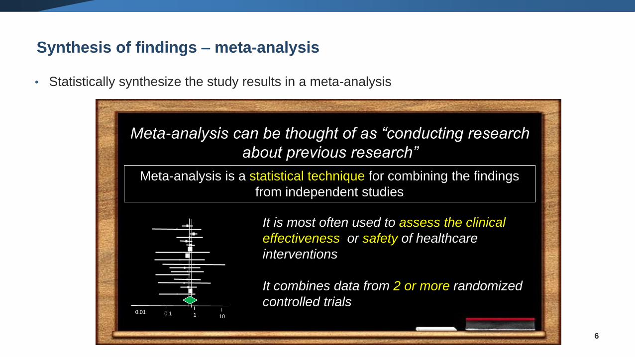
• Statistically synthesize the study results in a meta-analysis
Meta-analysis can be thought of as “conducting research
about previous research”
It is most often used to assess the clinical
effectiveness or safety of healthcare
interventions
It combines data from 2 or more randomized
controlled trials
Meta-analysis is a statistical technique for combining the findings
from independent studies
Synthesis of findings - Why perform a meta-analysis?
• To increase power/precision
• To reduce problems of interpretation due to sampling
variation
• To answer questions not posed by the individual studies
• To settle controversies arising from conflicting studies
7
Synthesis of findings - Basic principles of meta-analysis
• Participants in one study are not directly compared with those in another
• Each study is analysed separately
• Summary statistics are combined to give the meta-analysis estimate
• Each study is weighted according to the information it provides (usually the inverse
of its variance)
• Larger studies are given greater weight, and hence their influence on the meta-
analysis effect estimate is greater8
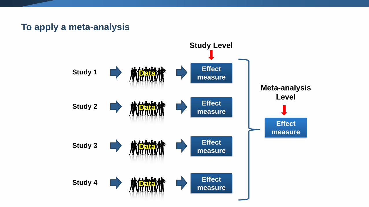
Study 1 DataEffect
measure
Study 2 DataEffect
measure
Study 3 DataEffect
measure
Study 4 DataEffect
measure
Study Level
Effect
measure
Meta-analysis
Level
To apply a meta-analysis
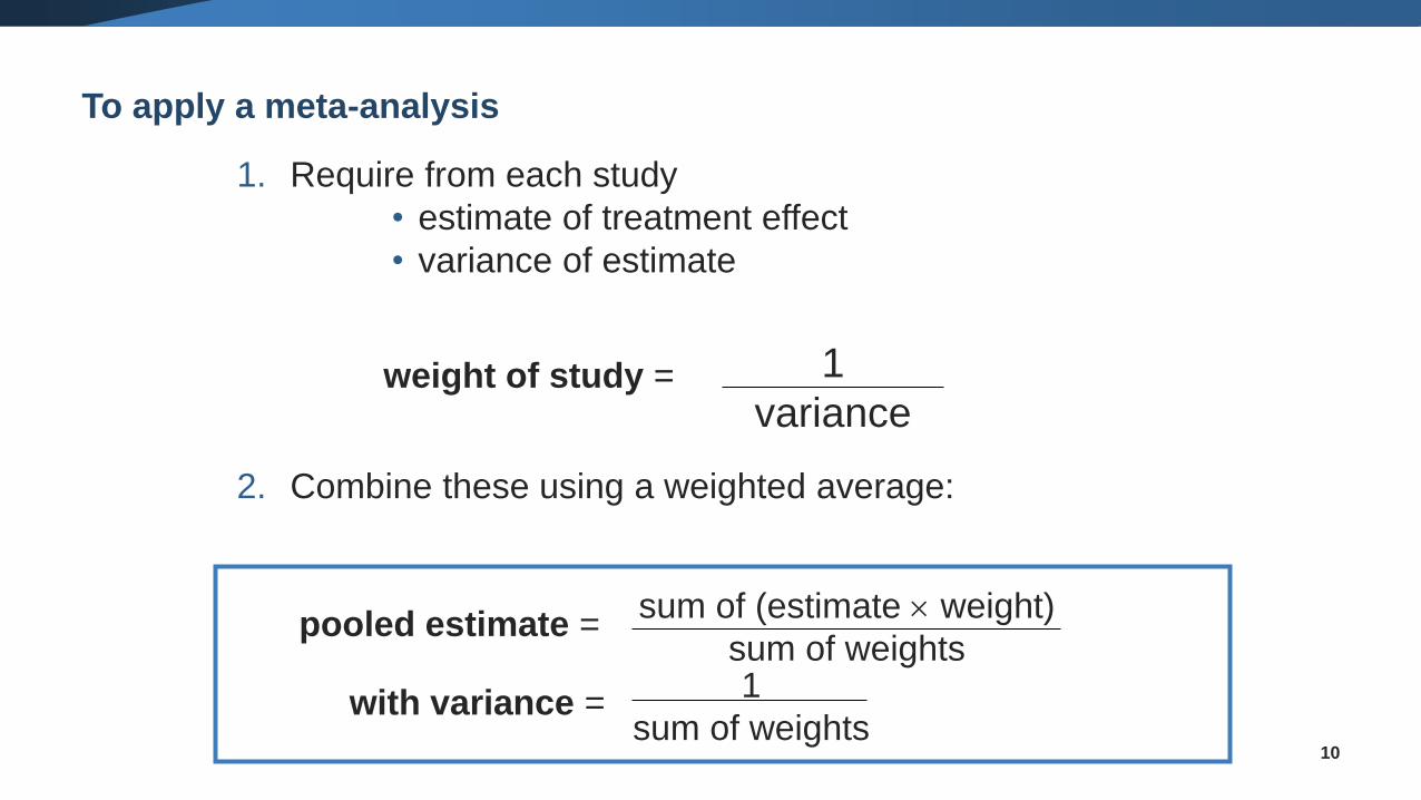
To apply a meta-analysis
10
1. Require from each study
• estimate of treatment effect
• variance of estimate
2. Combine these using a weighted average:
1
varianceweight of study =
1
sum of weights
sum of (estimate weight)
sum of weightspooled estimate =
with variance =
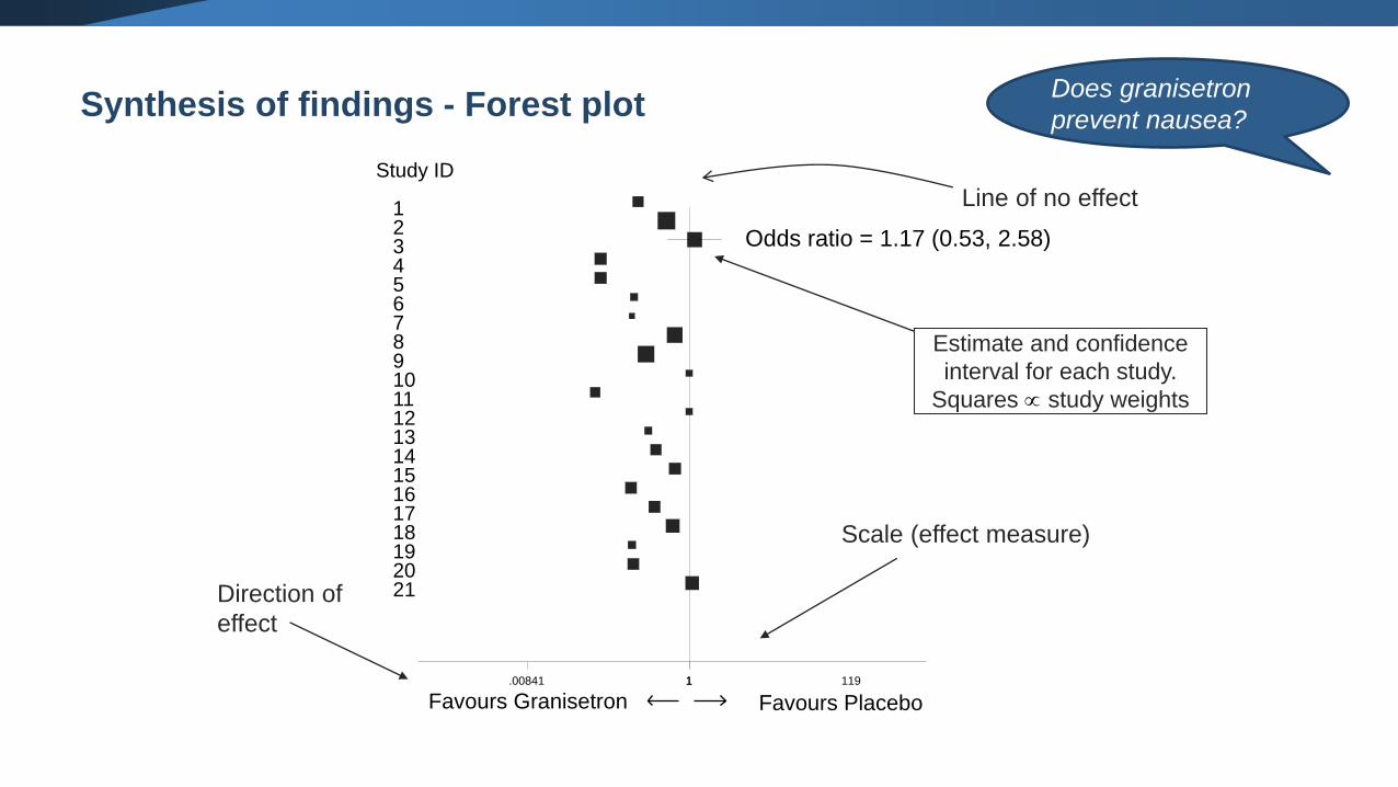
Synthesis of findings - Forest plotDoes granisetron
prevent nausea?
19
6
4
15
3
17
9
7
10
18
8
11
Study ID
21
12
20
13
1
16
14
2
5
Odds ratio = 1.17 (0.53, 2.58)
1.00841 1 119
Direction of
effect
Scale (effect measure)
Line of no effect
Favours Granisetron Favours Placebo
Estimate and confidence
interval for each study.
Squares study weights
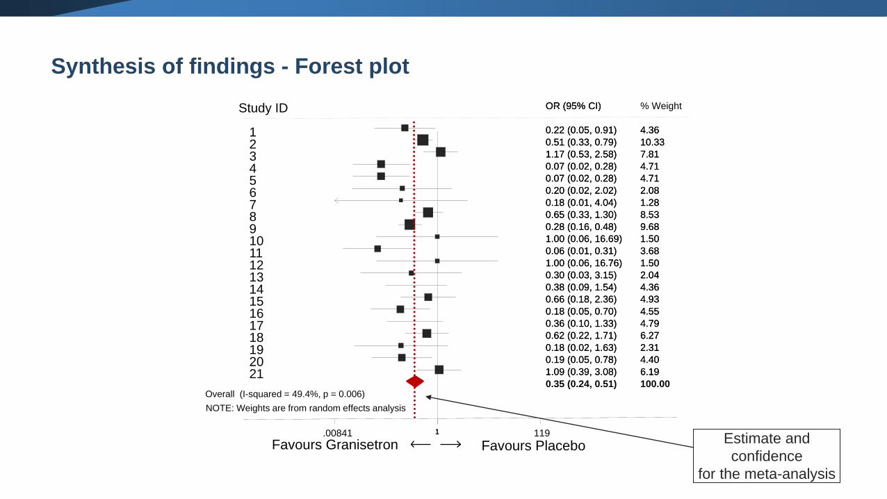
Synthesis of findings - Forest plot
NOTE: Weights are from random effects analysis
Overall (I-squared = 49.4%, p = 0.006)
19
6
4
15
3
17
9
7
10
18
8
11
21
12
20
13
1
16
14
2
5
0.18 (0.02, 1.63)
0.20 (0.02, 2.02)
0.07 (0.02, 0.28)
0.66 (0.18, 2.36)
1.17 (0.53, 2.58)
0.36 (0.10, 1.33)
0.28 (0.16, 0.48)
0.18 (0.01, 4.04)
1.00 (0.06, 16.69)
0.62 (0.22, 1.71)
0.65 (0.33, 1.30)
0.06 (0.01, 0.31)
OR (95% CI)
1.09 (0.39, 3.08)
1.00 (0.06, 16.76)
0.19 (0.05, 0.78)
0.30 (0.03, 3.15)
0.22 (0.05, 0.91)
0.18 (0.05, 0.70)
0.38 (0.09, 1.54)
0.51 (0.33, 0.79)
0.07 (0.02, 0.28)
2.31
2.08
4.71
4.93
7.81
4.79
9.68
1.28
1.50
6.27
8.53
3.68
% Weight
6.19
1.50
4.40
2.04
4.36
4.55
4.36
10.33
4.71
0.35 (0.24, 0.51)
0.18 (0.02, 1.63)
0.20 (0.02, 2.02)
0.07 (0.02, 0.28)
0.66 (0.18, 2.36)
1.17 (0.53, 2.58)
0.36 (0.10, 1.33)
0.28 (0.16, 0.48)
0.18 (0.01, 4.04)
1.00 (0.06, 16.69)
0.62 (0.22, 1.71)
0.65 (0.33, 1.30)
0.06 (0.01, 0.31)
OR (95% CI)
1.09 (0.39, 3.08)
1.00 (0.06, 16.76)
0.19 (0.05, 0.78)
0.30 (0.03, 3.15)
0.22 (0.05, 0.91)
0.18 (0.05, 0.70)
0.38 (0.09, 1.54)
0.51 (0.33, 0.79)
0.07 (0.02, 0.28)
100.00
2.31
2.08
4.71
4.93
7.81
4.79
9.68
1.28
1.50
6.27
8.53
3.68
6.19
1.50
4.40
2.04
4.36
4.55
4.36
10.33
4.71
1.00841 1 119
Study ID
Estimate and
confidence
for the meta-analysis
Favours Granisetron Favours Placebo
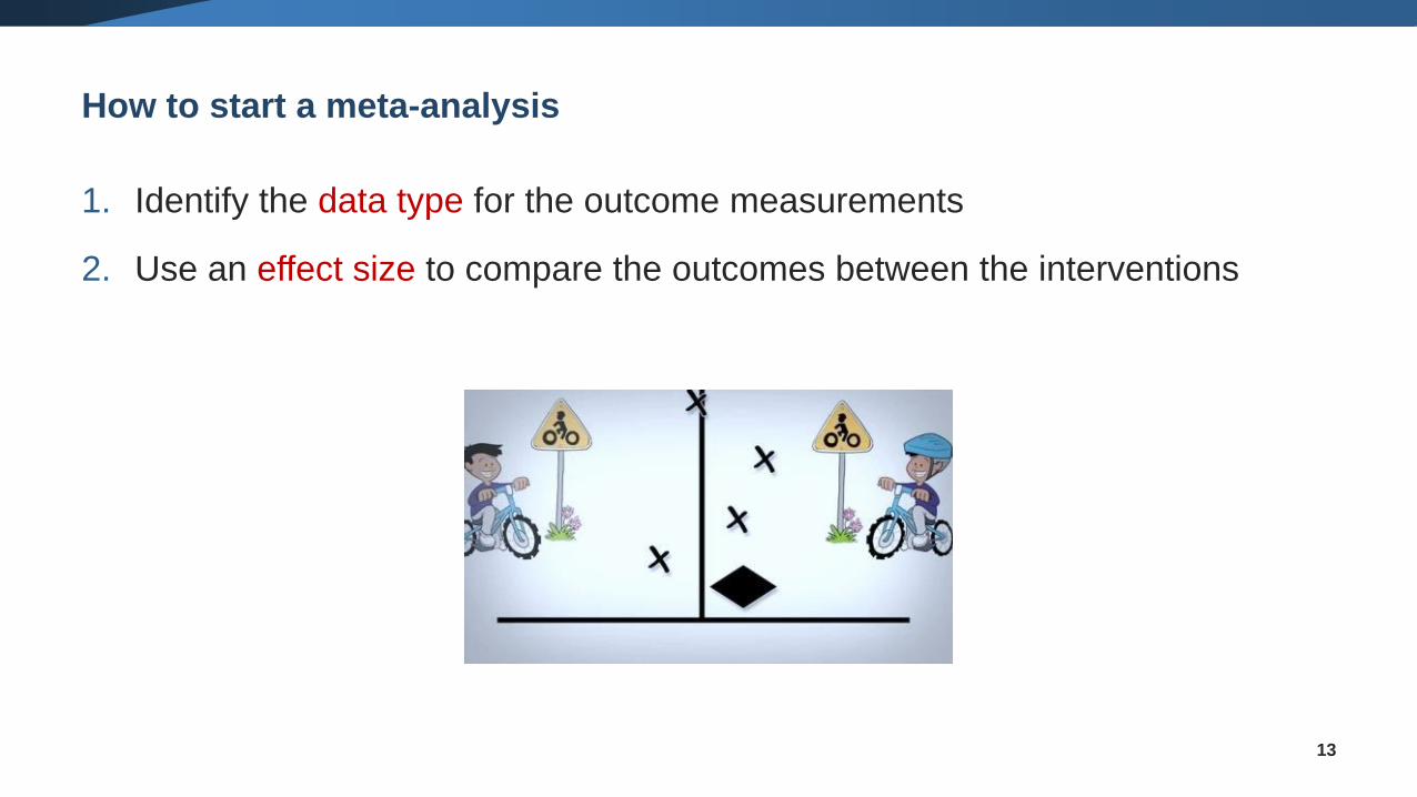
How to start a meta-analysis
1. Identify the data type for the outcome measurements
2. Use an effect size to compare the outcomes between the interventions
13
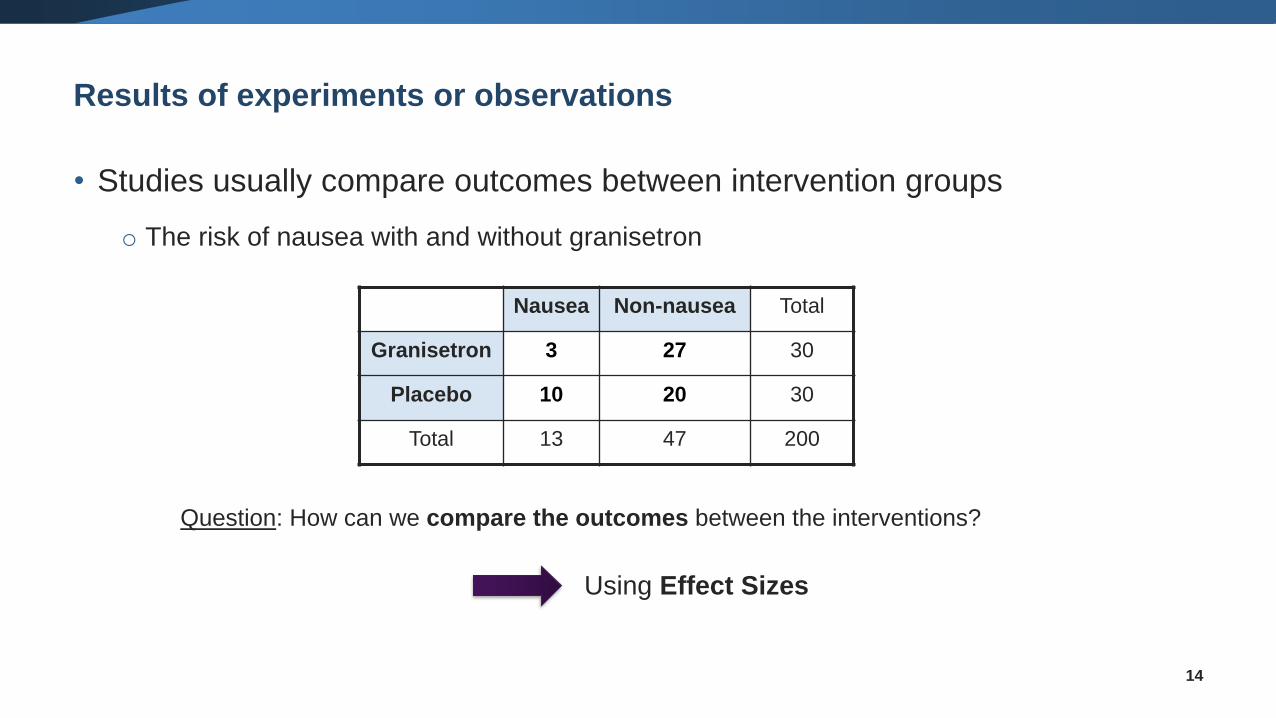
Results of experiments or observations
• Studies usually compare outcomes between intervention groups
o The risk of nausea with and without granisetron
14
Question: How can we compare the outcomes between the interventions?
Using Effect Sizes
Nausea Non-nausea Total
Granisetron 3 27 30
Placebo 10 20 30
Total 13 47 200
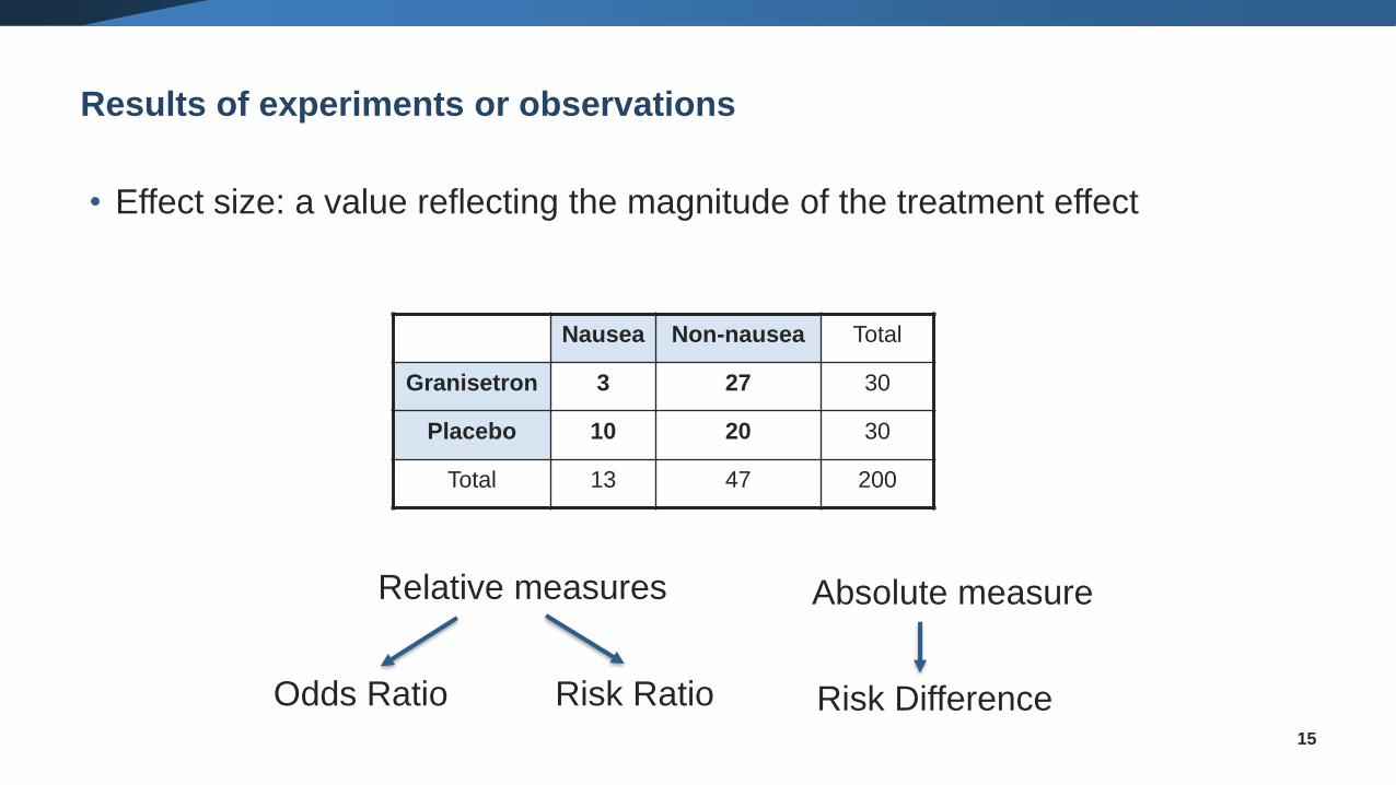
Results of experiments or observations
• Effect size: a value reflecting the magnitude of the treatment effect
15
Relative measures
Odds Ratio Risk Ratio
Absolute measure
Risk Difference
Nausea Non-nausea Total
Granisetron 3 27 30
Placebo 10 20 30
Total 13 47 200
Dichotomous data
16
• When the outcome for every participant is one of two possibilities
or events
❑ alive or dead
❑ healed or not healed
❑ pregnant or not pregnant
❑ …
17
What are dichotomous (or binary) outcomes?
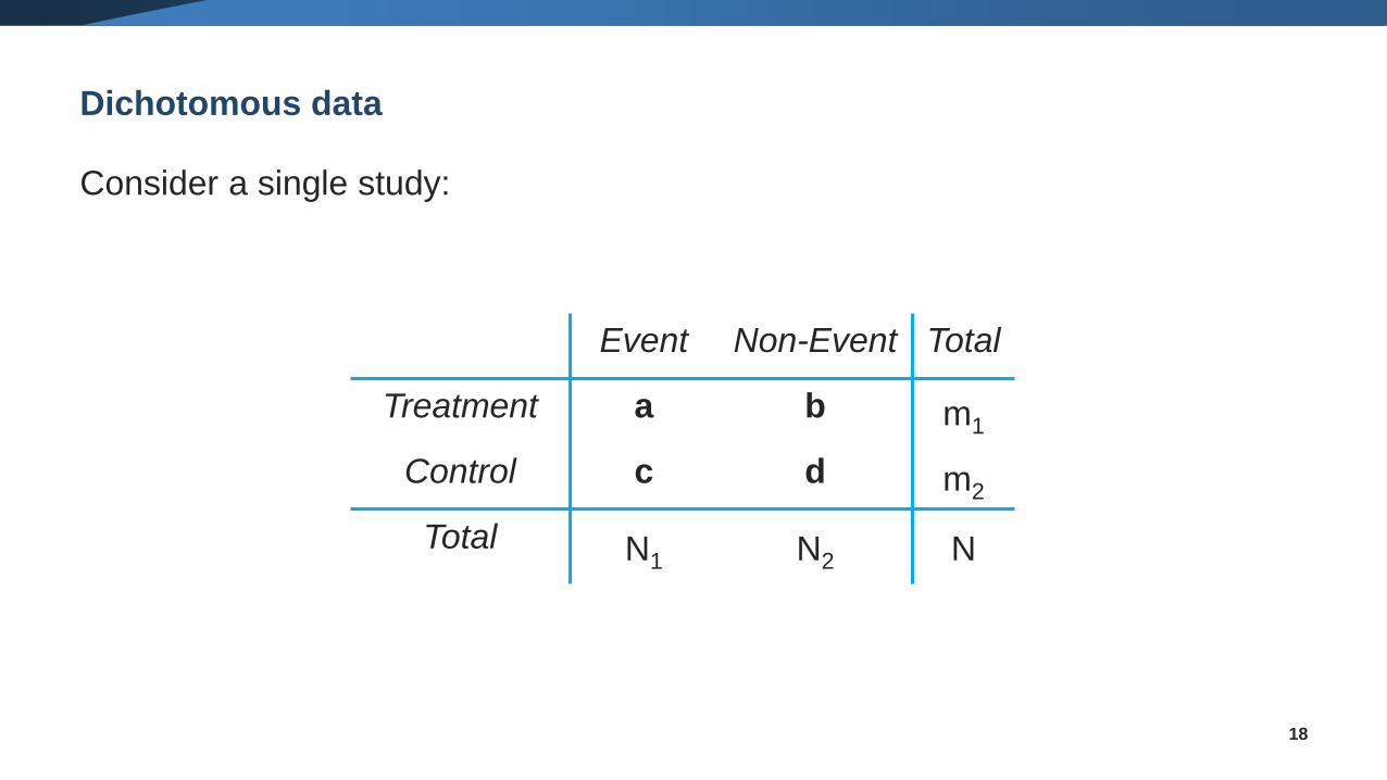
Dichotomous data
Consider a single study:
18
Event Non-Event Total
Treatment a b m1
Control c d m2
Total N1 N2 N
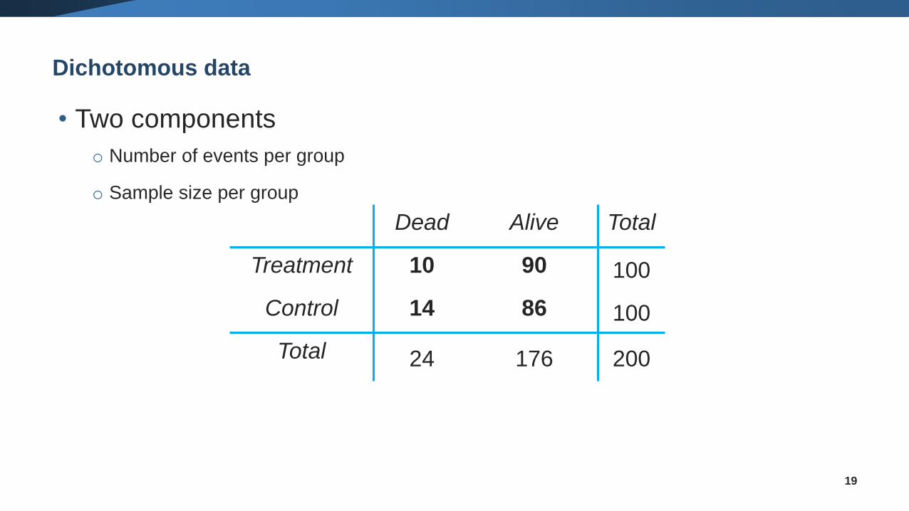
Dichotomous data
19
• Two components
o Number of events per group
o Sample size per group
Dead Alive Total
Treatment 10 90 100
Control 14 86 100
Total 24 176 200
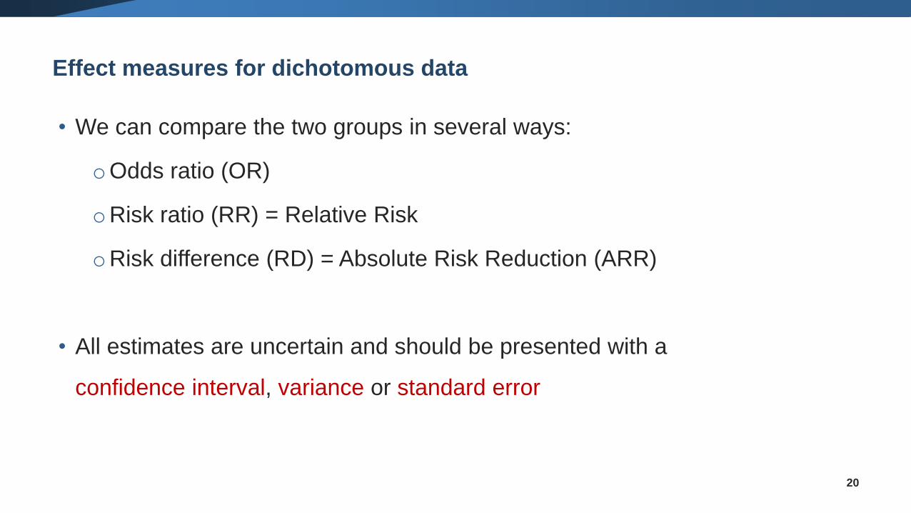
Effect measures for dichotomous data
• We can compare the two groups in several ways:
oOdds ratio (OR)
oRisk ratio (RR) = Relative Risk
oRisk difference (RD) = Absolute Risk Reduction (ARR)
• All estimates are uncertain and should be presented with a
confidence interval, variance or standard error
20
21
Risk and odds are just different ways of
expressing how likely an event is
Risk vs Odds
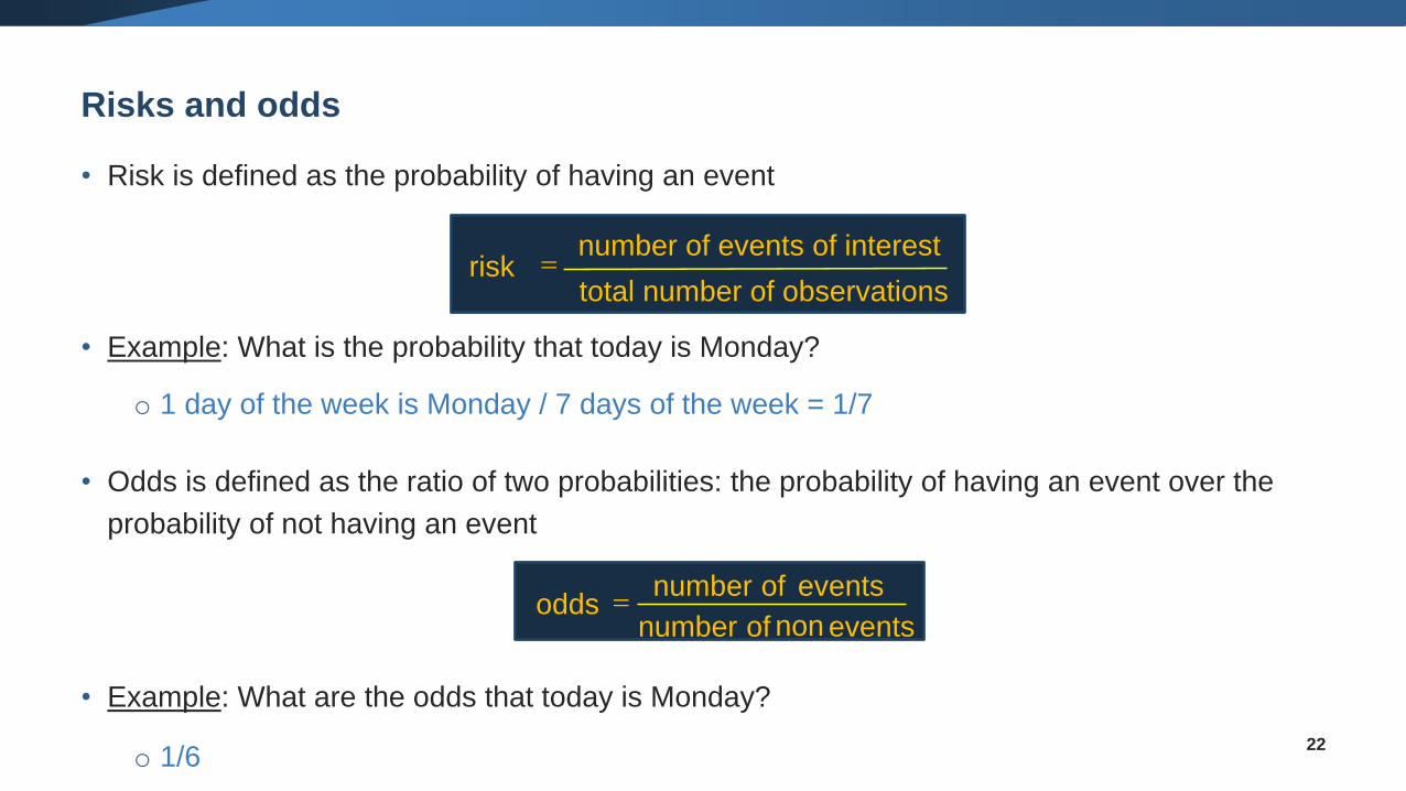
Risks and odds
• Risk is defined as the probability of having an event
• Example: What is the probability that today is Monday?
o 1 day of the week is Monday / 7 days of the week = 1/7
• Odds is defined as the ratio of two probabilities: the probability of having an event over the
probability of not having an event
• Example: What are the odds that today is Monday?
o 1/622
total number of observations
number of events of interestrisk =
non eventsofnumber
eventsofnumberodds =
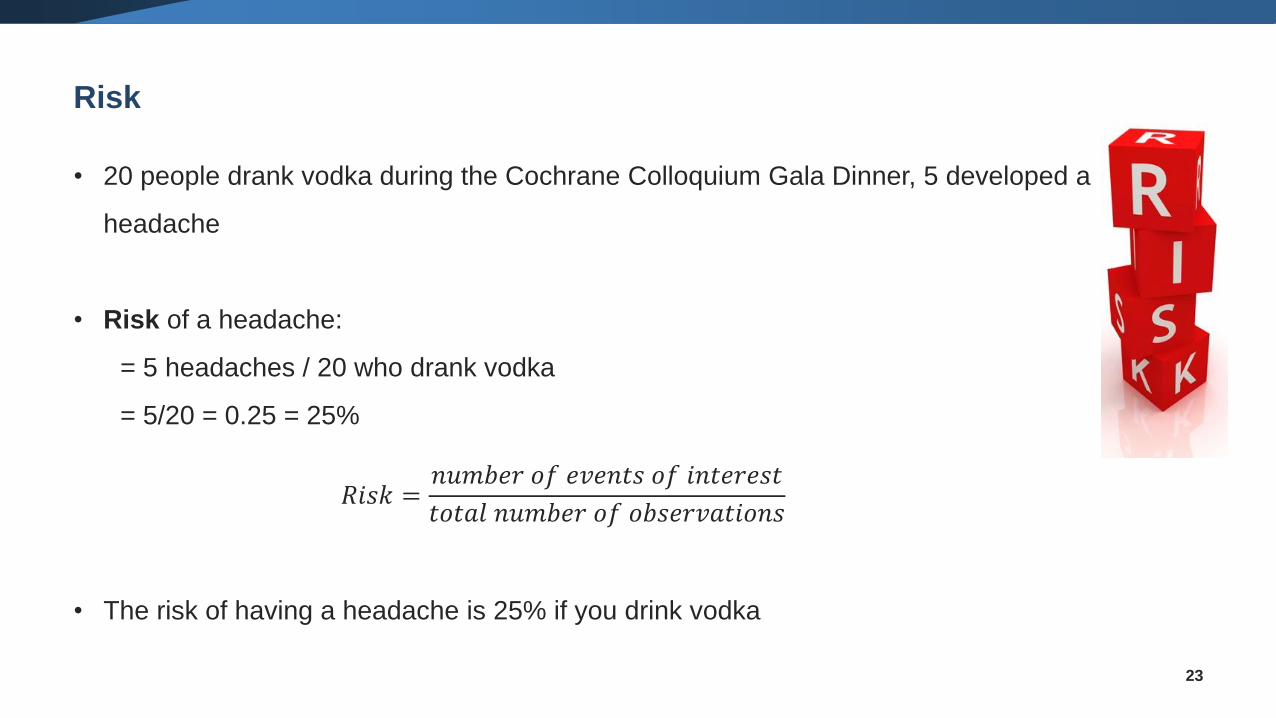
• 20 people drank vodka during the Cochrane Colloquium Gala Dinner, 5 developed a
headache
• Risk of a headache:
= 5 headaches / 20 who drank vodka
= 5/20 = 0.25 = 25%
𝑅𝑖𝑠𝑘 =𝑛𝑢𝑚𝑏𝑒𝑟 𝑜𝑓 𝑒𝑣𝑒𝑛𝑡𝑠 𝑜𝑓 𝑖𝑛𝑡𝑒𝑟𝑒𝑠𝑡
𝑡𝑜𝑡𝑎𝑙 𝑛𝑢𝑚𝑏𝑒𝑟 𝑜𝑓 𝑜𝑏𝑠𝑒𝑟𝑣𝑎𝑡𝑖𝑜𝑛𝑠
• The risk of having a headache is 25% if you drink vodka
23
Risk
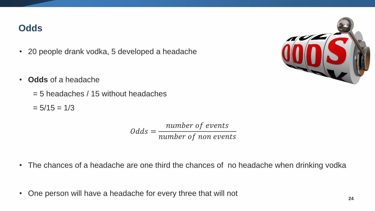
• 20 people drank vodka, 5 developed a headache
• Odds of a headache
= 5 headaches / 15 without headaches
= 5/15 = 1/3
𝑂𝑑𝑑𝑠 =𝑛𝑢𝑚𝑏𝑒𝑟 𝑜𝑓 𝑒𝑣𝑒𝑛𝑡𝑠
𝑛𝑢𝑚𝑏𝑒𝑟 𝑜𝑓 𝑛𝑜𝑛 𝑒𝑣𝑒𝑛𝑡𝑠
• The chances of a headache are one third the chances of no headache when drinking vodka
• One person will have a headache for every three that will not24
Odds
25
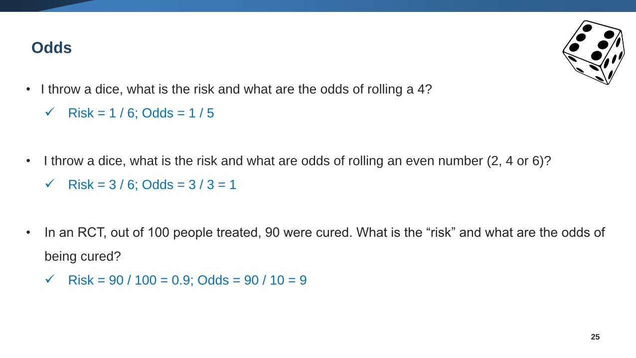
• I throw a dice, what is the risk and what are the odds of rolling a 4?
✓ Risk = 1 / 6; Odds = 1 / 5
• I throw a dice, what is the risk and what are odds of rolling an even number (2, 4 or 6)?
✓ Risk = 3 / 6; Odds = 3 / 3 = 1
• In an RCT, out of 100 people treated, 90 were cured. What is the “risk” and what are the odds of
being cured?
✓ Risk = 90 / 100 = 0.9; Odds = 90 / 10 = 9
Odds
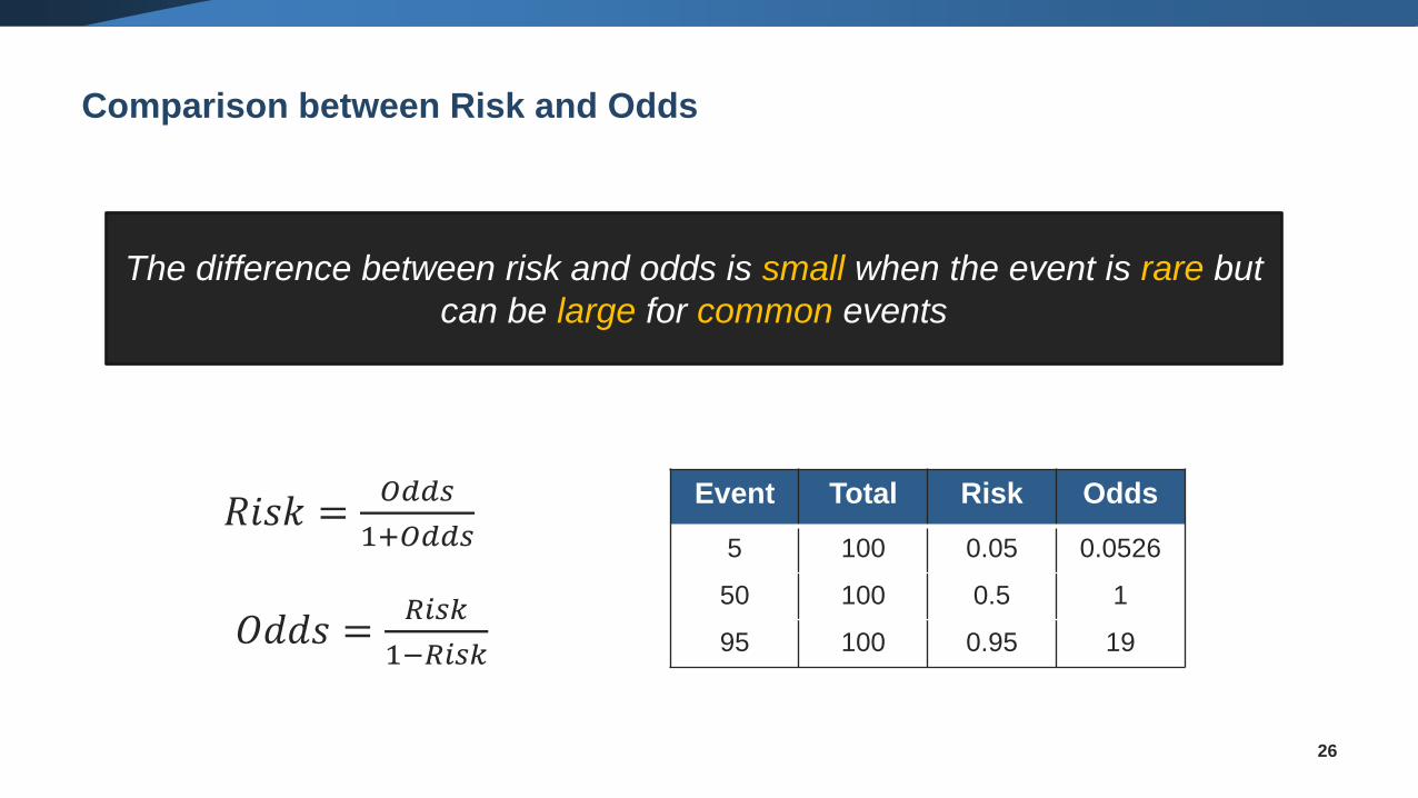
Comparison between Risk and Odds
26
Event Total Risk Odds
5 100 0.05 0.0526
50 100 0.5 1
95 100 0.95 19
The difference between risk and odds is small when the event is rare but
can be large for common events
𝑅𝑖𝑠𝑘 =𝑂𝑑𝑑𝑠
1+𝑂𝑑𝑑𝑠
𝑂𝑑𝑑𝑠 =𝑅𝑖𝑠𝑘
1−𝑅𝑖𝑠𝑘
27
Q: Does vodka lead to an increased chance of having a headache?
A: We need to compare people drinking vodka with a control group,
e.g. people drinking water
28
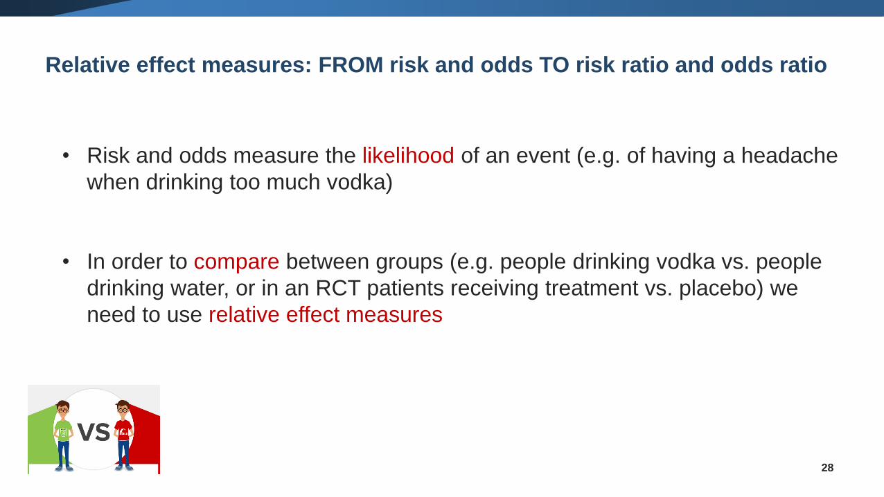
• Risk and odds measure the likelihood of an event (e.g. of having a headache
when drinking too much vodka)
• In order to compare between groups (e.g. people drinking vodka vs. people
drinking water, or in an RCT patients receiving treatment vs. placebo) we
need to use relative effect measures
Relative effect measures: FROM risk and odds TO risk ratio and odds ratio

29
Group A
(treatment)
Risk (treatment group) Risk (control group)
Group B
(control)
𝑅𝑖𝑠𝑘 𝑅𝑎𝑡𝑖𝑜 =𝑅𝑖𝑠𝑘 𝑖𝑛 𝑡𝑟𝑒𝑎𝑡𝑚𝑒𝑛𝑡 𝑔𝑟𝑜𝑢𝑝
𝑅𝑖𝑠𝑘 𝑖𝑛 𝑐𝑜𝑛𝑡𝑟𝑜𝑙 𝑔𝑟𝑜𝑢𝑝
Risk Ratio allows us to compare between two groups
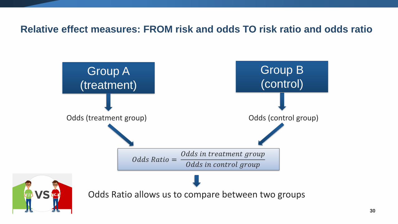
Relative effect measures: FROM risk and odds TO risk ratio and odds ratio
30
Group A
(treatment)
Group B
(control)
𝑂𝑑𝑑𝑠 𝑅𝑎𝑡𝑖𝑜 =𝑂𝑑𝑑𝑠 𝑖𝑛 𝑡𝑟𝑒𝑎𝑡𝑚𝑒𝑛𝑡 𝑔𝑟𝑜𝑢𝑝
𝑂𝑑𝑑𝑠 𝑖𝑛 𝑐𝑜𝑛𝑡𝑟𝑜𝑙 𝑔𝑟𝑜𝑢𝑝
Odds Ratio allows us to compare between two groups
Odds (treatment group) Odds (control group)
Relative effect measures: FROM risk and odds TO risk ratio and odds ratio
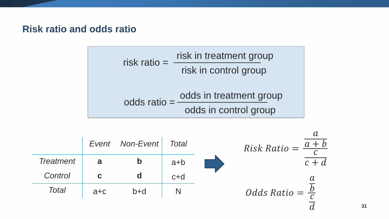
Risk ratio and odds ratio
31
odds ratio = odds in treatment group
odds in control group
risk ratio = risk in treatment group
risk in control group
Event Non-Event Total
Treatment a b a+b
Control c d c+d
Total a+c b+d N
𝑅𝑖𝑠𝑘 𝑅𝑎𝑡𝑖𝑜 =
𝑎𝑎 + 𝑏𝑐
𝑐 + 𝑑
𝑂𝑑𝑑𝑠 𝑅𝑎𝑡𝑖𝑜 =
𝑎𝑏𝑐𝑑
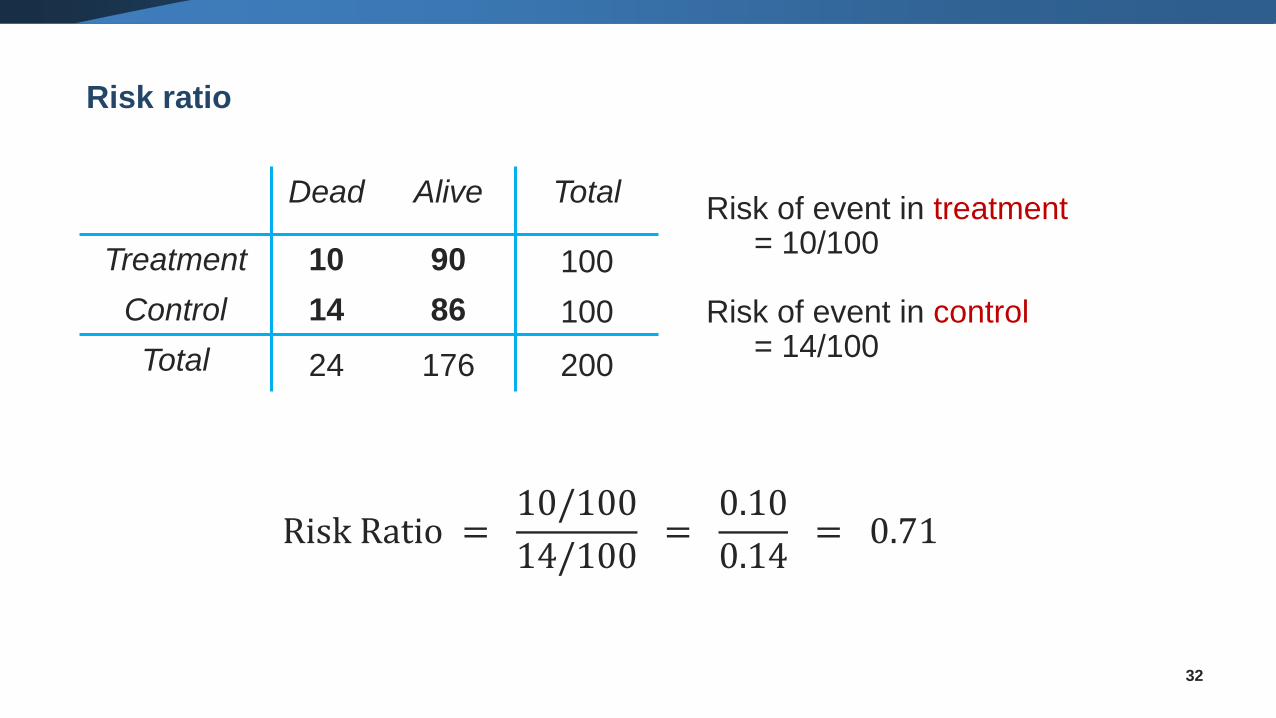
Risk ratio
32
Dead Alive Total
Treatment 10 90 100
Control 14 86 100
Total 24 176 200
Risk of event in treatment= 10/100
Risk of event in control= 14/100
Risk Ratio =10/100
14/100=
0.10
0.14= 0.71
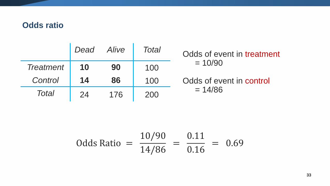
33
Odds of event in treatment= 10/90
Odds of event in control= 14/86
Dead Alive Total
Treatment 10 90 100
Control 14 86 100
Total 24 176 200
Odds ratio
Odds Ratio =10/90
14/86=
0.11
0.16= 0.69
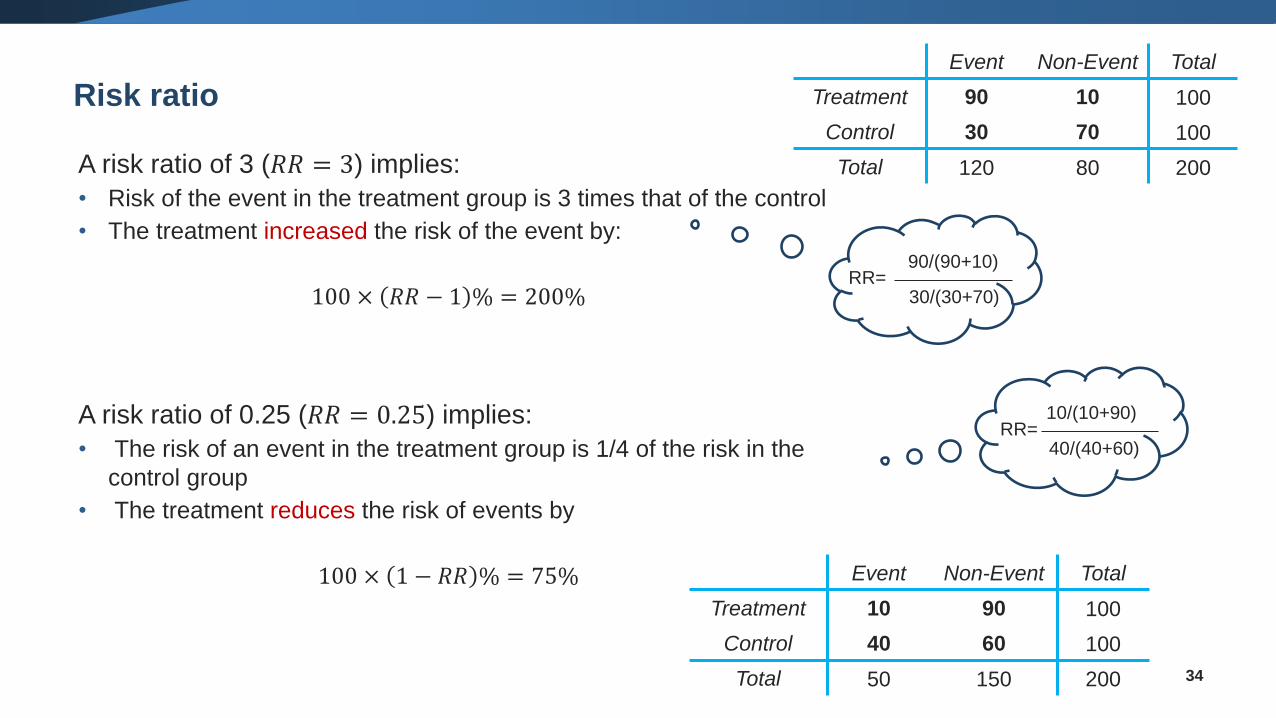
Risk ratio
34
A risk ratio of 3 (𝑅𝑅 = 3) implies:
• Risk of the event in the treatment group is 3 times that of the control
• The treatment increased the risk of the event by:
100 × 𝑅𝑅 − 1 % = 200%
A risk ratio of 0.25 (𝑅𝑅 = 0.25) implies:
• The risk of an event in the treatment group is 1/4 of the risk in the
control group
• The treatment reduces the risk of events by
100 × 1 − 𝑅𝑅 % = 75%
90/(90+10)
30/(30+70)RR=
10/(10+90)
40/(40+60)RR=
Event Non-Event Total
Treatment 90 10 100
Control 30 70 100
Total 120 80 200
Event Non-Event Total
Treatment 10 90 100
Control 40 60 100
Total 50 150 200
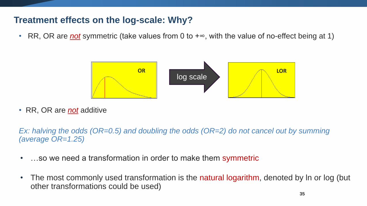
• RR, OR are not symmetric (take values from 0 to +∞, with the value of no-effect being at 1)
• RR, OR are not additive
Ex: halving the odds (OR=0.5) and doubling the odds (OR=2) do not cancel out by summing (average OR=1.25)
• …so we need a transformation in order to make them symmetric
• The most commonly used transformation is the natural logarithm, denoted by ln or log (but other transformations could be used)
OR LORlog scale
Treatment effects on the log-scale: Why?
35
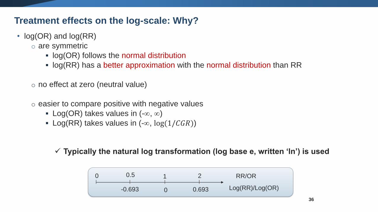
• log(OR) and log(RR)
o are symmetric
▪ log(OR) follows the normal distribution
▪ log(RR) has a better approximation with the normal distribution than RR
o no effect at zero (neutral value)
o easier to compare positive with negative values
▪ Log(OR) takes values in (-, )
▪ Log(RR) takes values in (-, log(1/𝐶𝐺𝑅))
✓ Typically the natural log transformation (log base e, written ‘ln’) is used
36
Log(RR)/Log(OR)
RR/OR1
0
20.50
0.693-0.693
Treatment effects on the log-scale: Why?
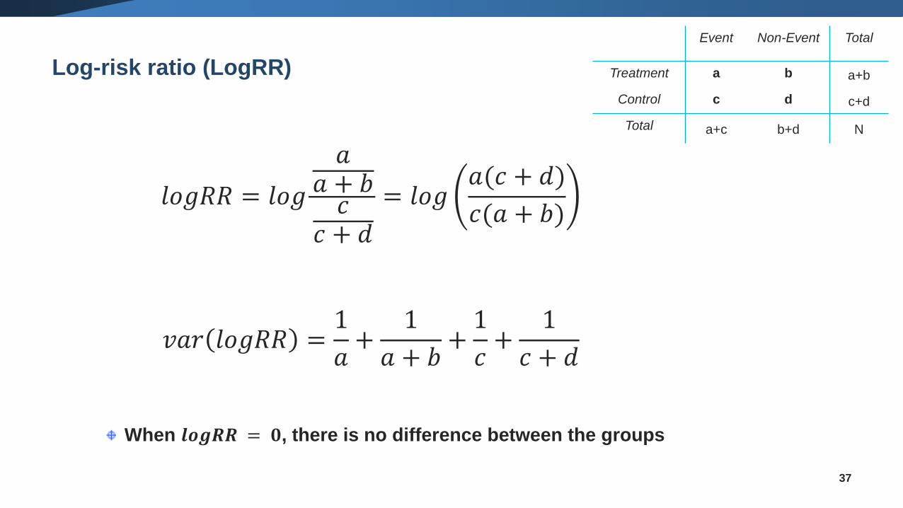
Log-risk ratio (LogRR)
37
𝑙𝑜𝑔𝑅𝑅 = 𝑙𝑜𝑔
𝑎𝑎 + 𝑏𝑐
𝑐 + 𝑑
= 𝑙𝑜𝑔𝑎(𝑐 + 𝑑)
𝑐(𝑎 + 𝑏)
𝑣𝑎𝑟 𝑙𝑜𝑔𝑅𝑅 =1
𝑎+
1
𝑎 + 𝑏+1
𝑐+
1
𝑐 + 𝑑
When 𝒍𝒐𝒈𝑹𝑹 = 𝟎, there is no difference between the groups
Event Non-Event Total
Treatment a b a+b
Control c d c+d
Total a+c b+d N
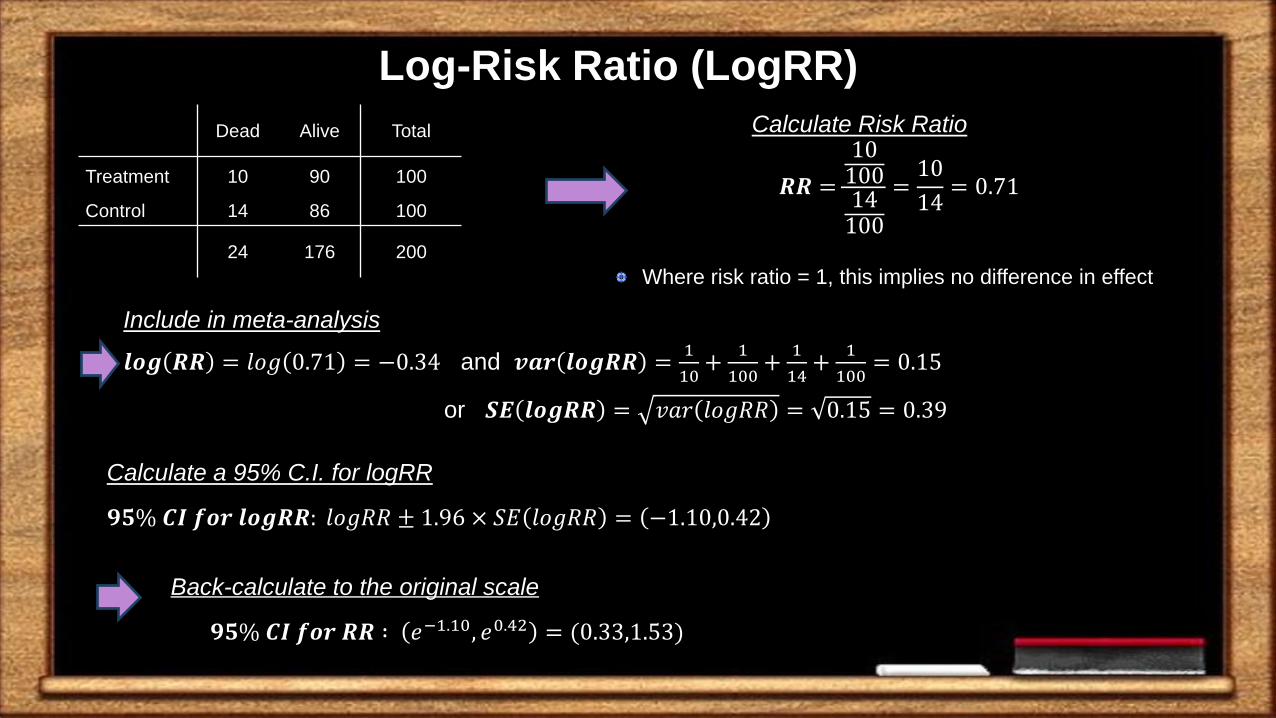
Back-calculate to the original scale
𝟗𝟓% 𝑪𝑰 𝒇𝒐𝒓 𝑹𝑹 ∶ 𝑒−1.10, 𝑒0.42 = (0.33,1.53)
Include in meta-analysis
𝒍𝒐𝒈 𝑹𝑹 = 𝑙𝑜𝑔 0.71 = −0.34 and 𝒗𝒂𝒓 𝒍𝒐𝒈𝑹𝑹 =1
10+
1
100+
1
14+
1
100= 0.15
or 𝑺𝑬 𝒍𝒐𝒈𝑹𝑹 = 𝑣𝑎𝑟 𝑙𝑜𝑔𝑅𝑅 = 0.15 = 0.39
Calculate Risk Ratio
𝑹𝑹 =
1010014100
=10
14= 0.71
Calculate a 95% C.I. for logRR
𝟗𝟓% 𝑪𝑰 𝒇𝒐𝒓 𝒍𝒐𝒈𝑹𝑹: 𝑙𝑜𝑔𝑅𝑅 ± 1.96 × 𝑆𝐸 𝑙𝑜𝑔𝑅𝑅 = −1.10,0.42
Dead Alive Total
Treatment 10 90 100
Control 14 86 100
24 176 200
Where risk ratio = 1, this implies no difference in effect
Log-Risk Ratio (LogRR)
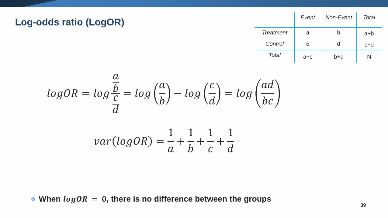
Log-odds ratio (LogOR)
39When 𝒍𝒐𝒈𝑶𝑹 = 𝟎, there is no difference between the groups
𝑙𝑜𝑔𝑂𝑅 = 𝑙𝑜𝑔
𝑎𝑏𝑐𝑑
= 𝑙𝑜𝑔𝑎
𝑏− 𝑙𝑜𝑔
𝑐
𝑑= 𝑙𝑜𝑔
𝑎𝑑
𝑏𝑐
𝑣𝑎𝑟 𝑙𝑜𝑔𝑂𝑅 =1
𝑎+1
𝑏+1
𝑐+1
𝑑
Event Non-Event Total
Treatment a b a+b
Control c d c+d
Total a+c b+d N
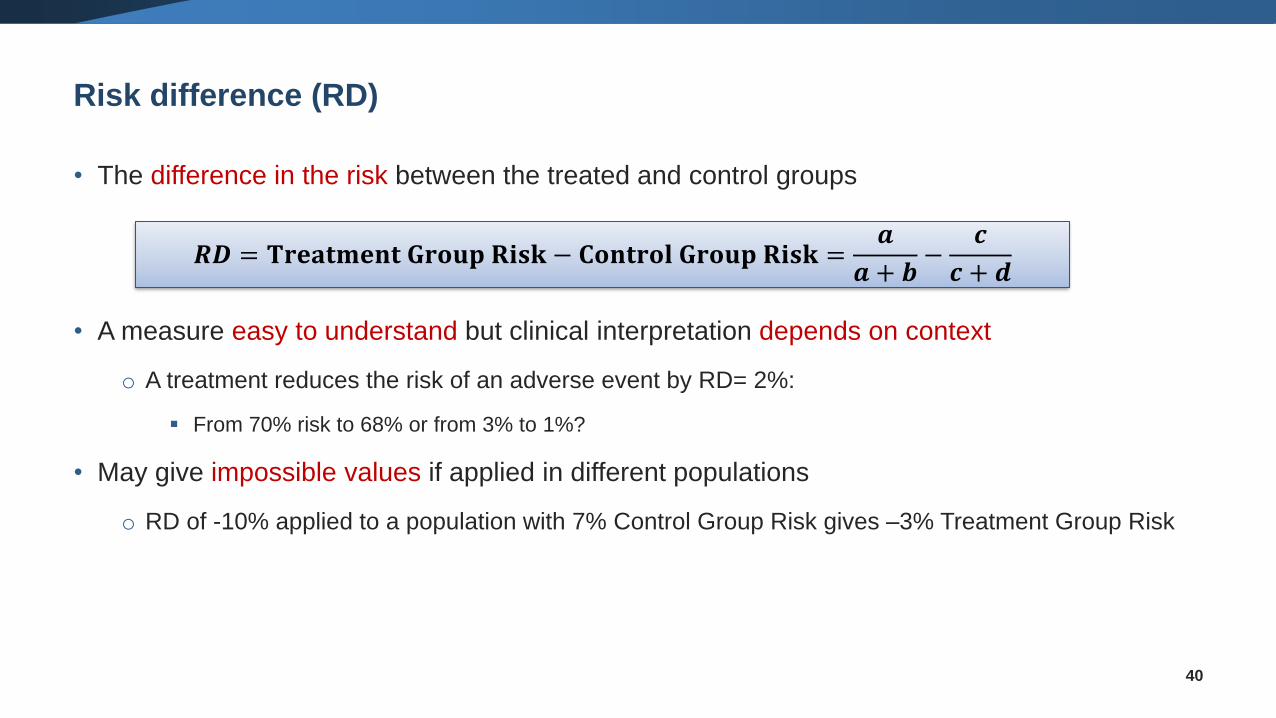
Risk difference (RD)
• The difference in the risk between the treated and control groups
• A measure easy to understand but clinical interpretation depends on context
o A treatment reduces the risk of an adverse event by RD= 2%:
▪ From 70% risk to 68% or from 3% to 1%?
• May give impossible values if applied in different populations
o RD of -10% applied to a population with 7% Control Group Risk gives –3% Treatment Group Risk
40
𝑹𝑫 = 𝐓𝐫𝐞𝐚𝐭𝐦𝐞𝐧𝐭 𝐆𝐫𝐨𝐮𝐩 𝐑𝐢𝐬𝐤 − 𝐂𝐨𝐧𝐭𝐫𝐨𝐥 𝐆𝐫𝐨𝐮𝐩 𝐑𝐢𝐬𝐤 =𝒂
𝒂 + 𝒃−
𝒄
𝒄 + 𝒅
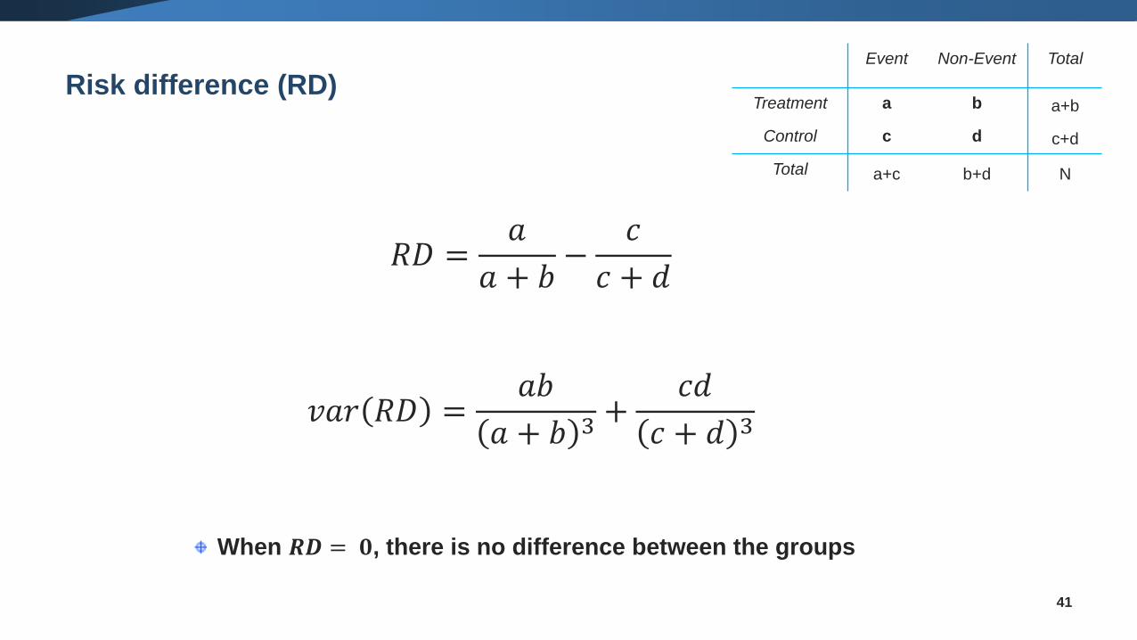
Risk difference (RD)
41
𝑅𝐷 =𝑎
𝑎 + 𝑏−
𝑐
𝑐 + 𝑑
𝑣𝑎𝑟 𝑅𝐷 =𝑎𝑏
𝑎 + 𝑏 3+
𝑐𝑑
𝑐 + 𝑑 3
When 𝑹𝑫 = 𝟎, there is no difference between the groups
Event Non-Event Total
Treatment a b a+b
Control c d c+d
Total a+c b+d N
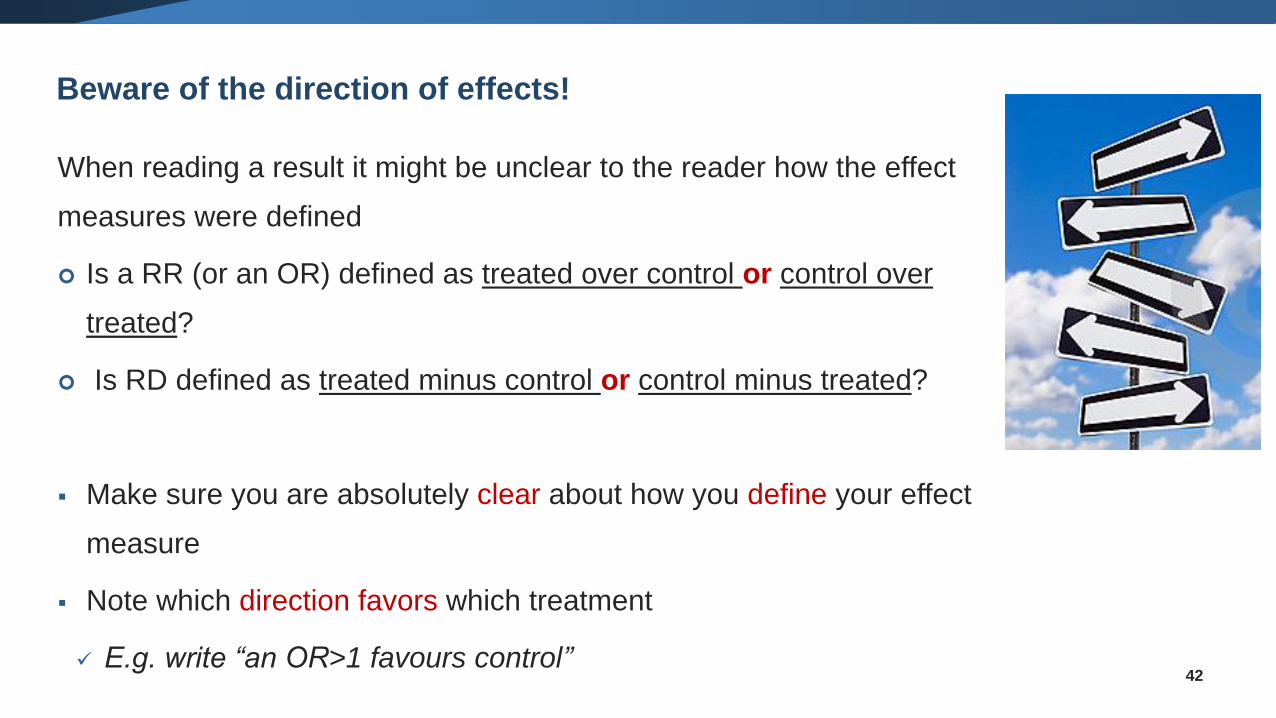
42
When reading a result it might be unclear to the reader how the effect
measures were defined
Is a RR (or an OR) defined as treated over control or control over
treated?
Is RD defined as treated minus control or control minus treated?
▪ Make sure you are absolutely clear about how you define your effect
measure
▪ Note which direction favors which treatment
✓ E.g. write “an OR>1 favours control”
Beware of the direction of effects!
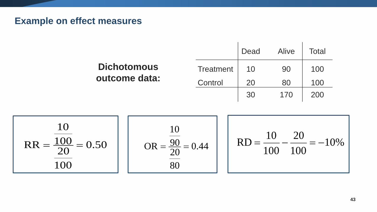
Dichotomous
outcome data:
0.50
100
20100
10
RR == 0.44
80
2090
10
OR == 10%100
20
100
10 RD −=−=
43
Dead Alive Total
Treatment 10 90 100
Control 20 80 100
30 170 200
Example on effect measures
• Communication of effect
✓users must be able to understand and apply the result
• Consistency of effect
✓applicable to all populations and contexts
• Mathematical properties
44
Choosing an effect measure
• OR is hard to understand, often misinterpreted
• RR is easier, but
✓It can mean a very small or very big change, depending on the
underlying risk
✓It can be very different if we switch the outcome
• RD is easiest
✓absolute measure of actual change in risk
45
Communication
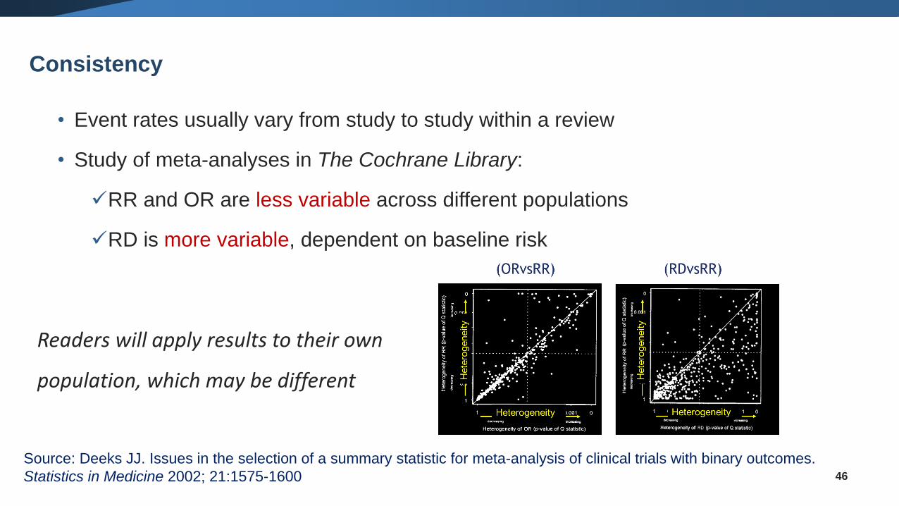
• Event rates usually vary from study to study within a review
• Study of meta-analyses in The Cochrane Library:
✓RR and OR are less variable across different populations
✓RD is more variable, dependent on baseline risk
46
Source: Deeks JJ. Issues in the selection of a summary statistic for meta-analysis of clinical trials with binary outcomes.
Statistics in Medicine 2002; 21:1575-1600
Consistency
Readers will apply results to their own
population, which may be different
• Defining the event
✓Good or bad, presence or absence?
✓Think carefully and choose in advance
✓OR and RD are stable either way, RR varies
47
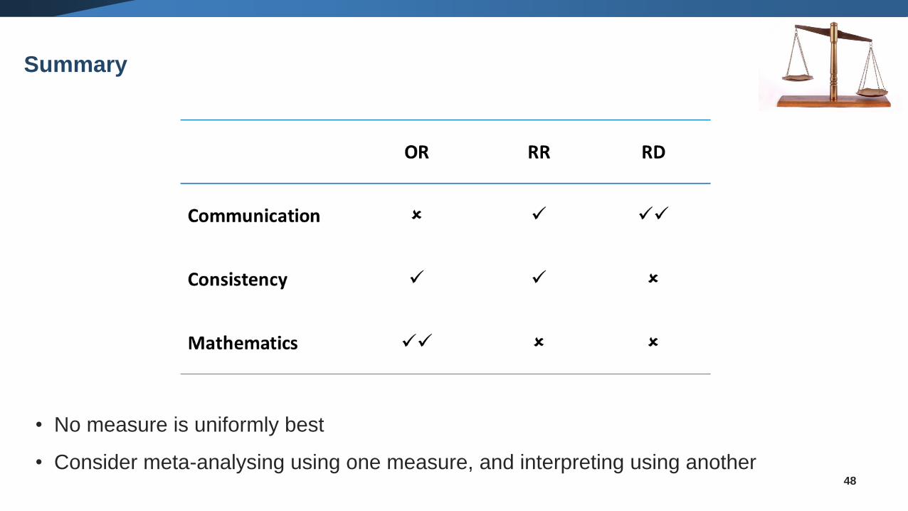
Mathematical Properties
48
• No measure is uniformly best
• Consider meta-analysing using one measure, and interpreting using another
Summary
• Inverse Variance Method (IV)
• Mantel-Haenszel (MH)
• Peto Odds Ratio
49
Methods for meta-analysis of dichotomous outcomes
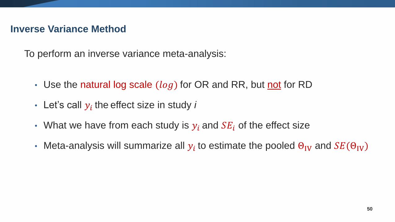
To perform an inverse variance meta-analysis:
• Use the natural log scale (𝑙𝑜𝑔) for OR and RR, but not for RD
• Let’s call 𝑦𝑖 the effect size in study i
• What we have from each study is 𝑦𝑖 and 𝑆𝐸𝑖 of the effect size
• Meta-analysis will summarize all 𝑦𝑖 to estimate the pooled ΘIV and 𝑆𝐸(ΘIV)
50
Inverse Variance Method
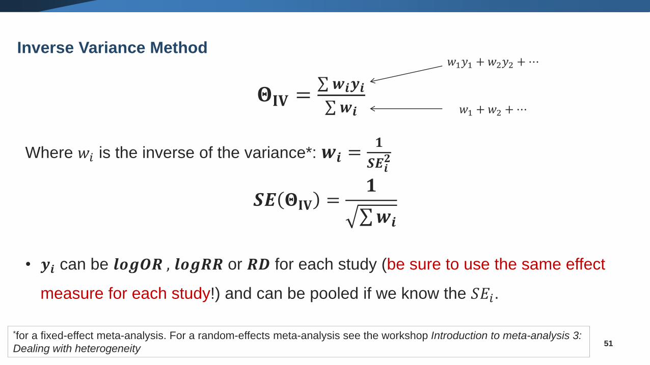
𝚯𝐈𝐕 =σ 𝒘𝒊𝒚𝒊σ 𝒘𝒊
Where 𝑤𝑖 is the inverse of the variance*: 𝒘𝒊 =𝟏
𝑺𝑬𝒊𝟐
𝑺𝑬 𝚯𝐈𝐕 =𝟏
σ𝒘𝒊
• 𝒚𝒊 can be 𝒍𝒐𝒈𝑶𝑹 , 𝒍𝒐𝒈𝑹𝑹 or 𝑹𝑫 for each study (be sure to use the same effect
measure for each study!) and can be pooled if we know the 𝑆𝐸𝑖.
51
𝑤1𝑦1 + 𝑤2𝑦2 +⋯
𝑤1 + 𝑤2 +⋯
*for a fixed-effect meta-analysis. For a random-effects meta-analysis see the workshop Introduction to meta-analysis 3:
Dealing with heterogeneity
Inverse Variance Method
52
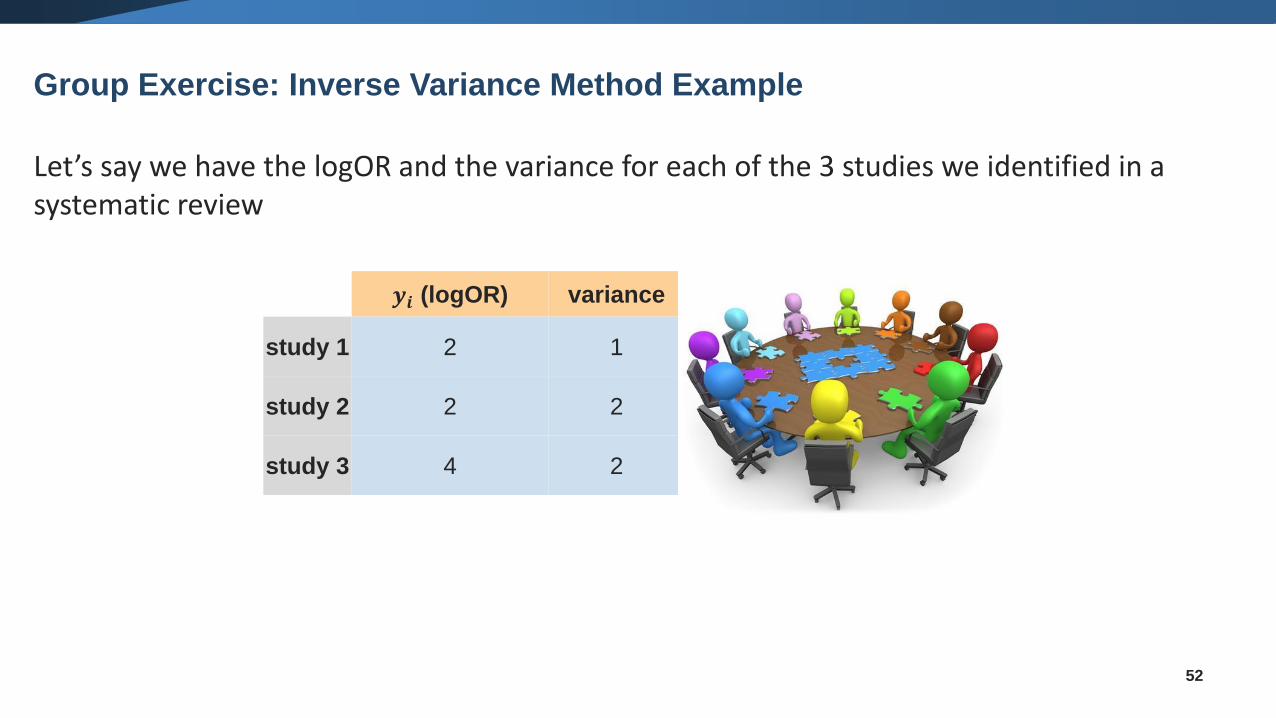
Let’s say we have the logOR and the variance for each of the 3 studies we identified in a systematic review
Group Exercise: Inverse Variance Method Example
𝒚𝒊 (logOR) variance 𝒘𝒊 𝒘𝒊𝒚𝒊
study 1 2 1 1 2
study 2 2 2 0.5 1
study 3 4 2 0.5 2
53
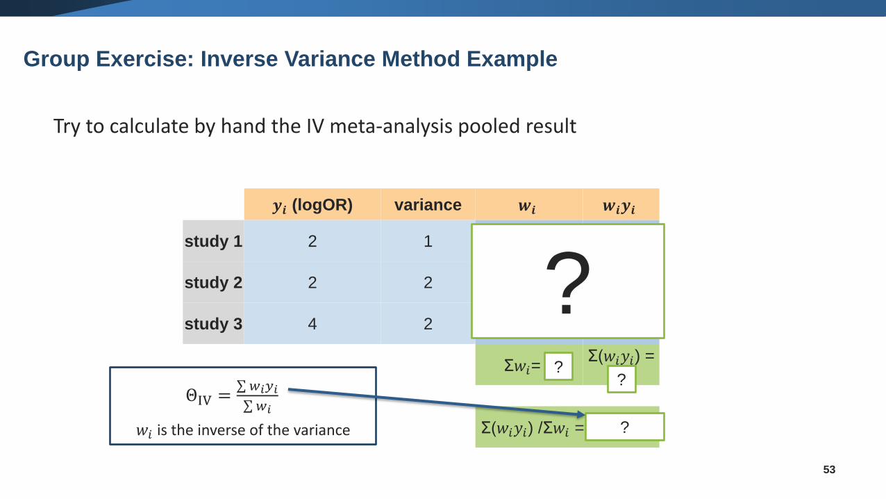
𝒚𝒊 (logOR) variance 𝒘𝒊 𝒘𝒊𝒚𝒊
study 1 2 1 1 2
study 2 2 2 0.5 1
study 3 4 2 0.5 2
Σ𝑤𝑖= 2Σ(𝑤𝑖𝑦𝑖) =
5
Σ(𝑤𝑖𝑦𝑖) /Σ𝑤𝑖 = 5/2 = 2.5
??
?
?
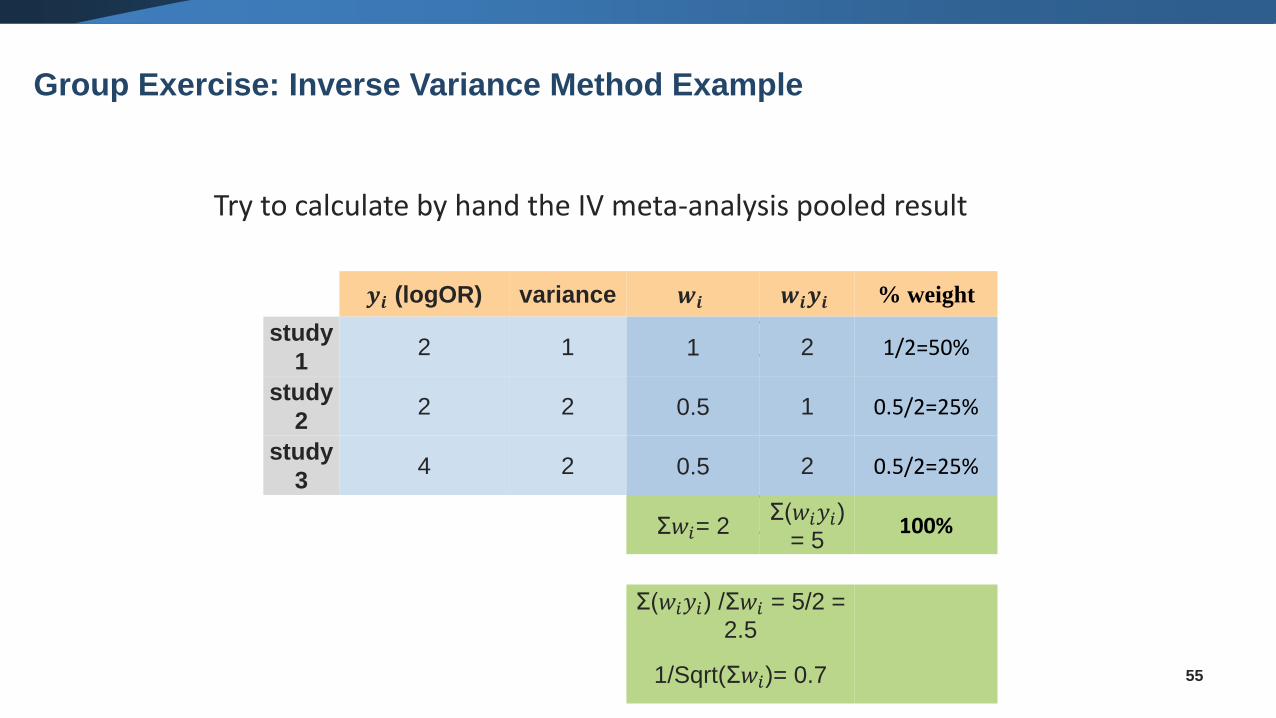
Try to calculate by hand the IV meta-analysis pooled result
ΘIV =σ 𝑤𝑖𝑦𝑖σ 𝑤𝑖
𝑤𝑖 is the inverse of the variance
Group Exercise: Inverse Variance Method Example
54
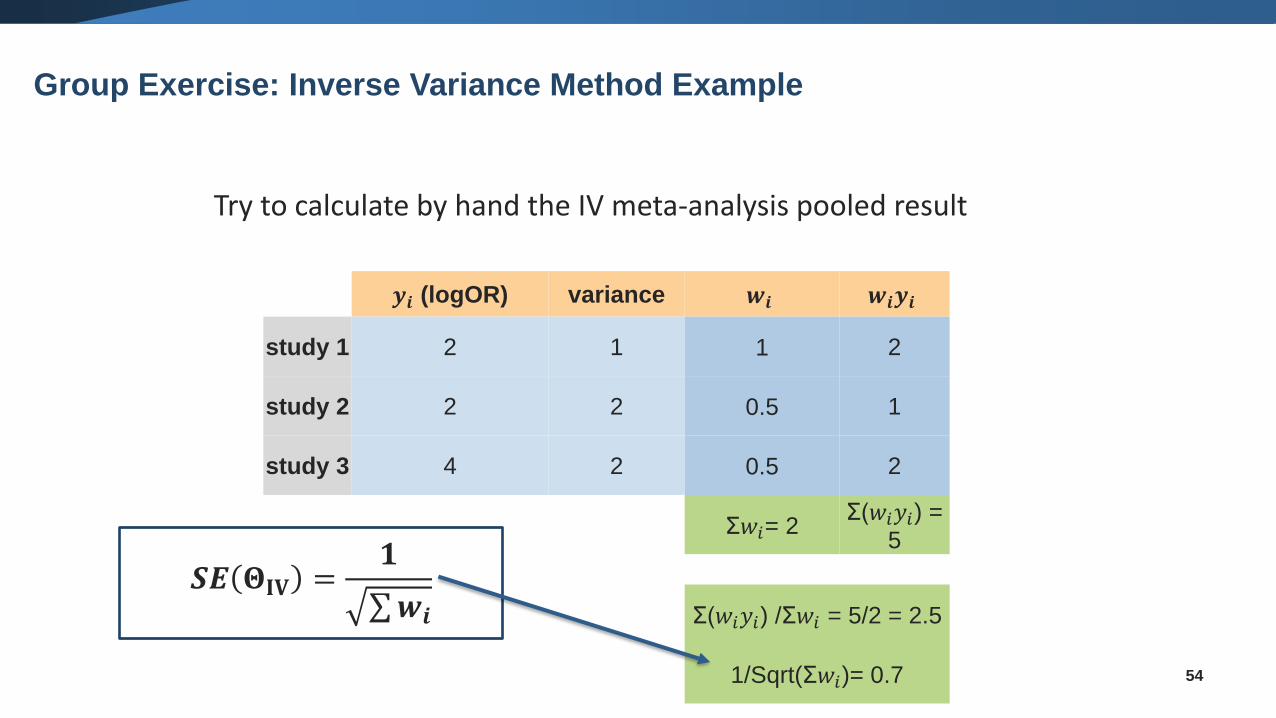
Try to calculate by hand the IV meta-analysis pooled result
𝒚𝒊 (logOR) variance 𝒘𝒊 𝒘𝒊𝒚𝒊
study 1 2 1 1 2
study 2 2 2 0.5 1
study 3 4 2 0.5 2
Σ𝑤𝑖= 2Σ(𝑤𝑖𝑦𝑖) =
5
Σ(𝑤𝑖𝑦𝑖) /Σ𝑤𝑖 = 5/2 = 2.5
1/Sqrt(Σ𝑤𝑖)= 0.7
𝑺𝑬 𝚯𝐈𝐕 =𝟏
σ𝒘𝒊
Group Exercise: Inverse Variance Method Example
55
Try to calculate by hand the IV meta-analysis pooled result
𝒚𝒊 (logOR) variance 𝒘𝒊 𝒘𝒊𝒚𝒊 % weight
study
12 1 1 2 1/2=50%
study
22 2 0.5 1 0.5/2=25%
study
34 2 0.5 2 0.5/2=25%
Σ𝑤𝑖= 2Σ(𝑤𝑖𝑦𝑖)
= 5100%
Σ(𝑤𝑖𝑦𝑖) /Σ𝑤𝑖 = 5/2 =
2.5
1/Sqrt(Σ𝑤𝑖)= 0.7
Group Exercise: Inverse Variance Method Example
56
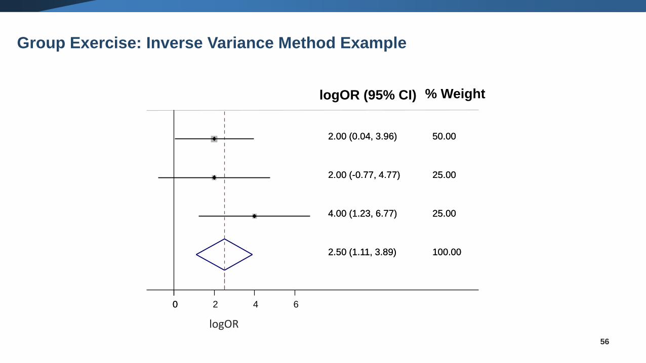
2.50 (1.11, 3.89)
2.00 (0.04, 3.96)
4.00 (1.23, 6.77)
2.00 (-0.77, 4.77)
100.00
% Weight
50.00
25.00
25.00
2.50 (1.11, 3.89)
logOR (95% CI)
2.00 (0.04, 3.96)
4.00 (1.23, 6.77)
2.00 (-0.77, 4.77)
100.00
50.00
25.00
25.00
00 2 4 6
logOR
Group Exercise: Inverse Variance Method Example
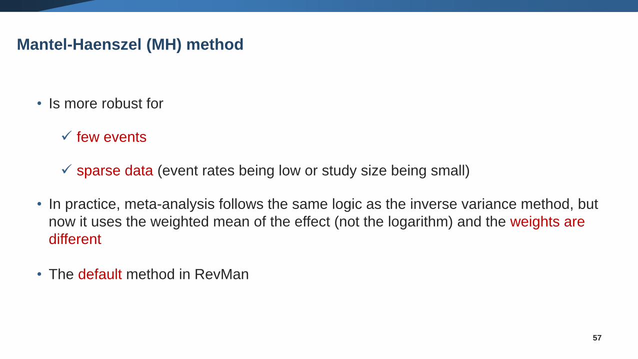
• Is more robust for
✓ few events
✓ sparse data (event rates being low or study size being small)
• In practice, meta-analysis follows the same logic as the inverse variance method, but
now it uses the weighted mean of the effect (not the logarithm) and the weights are
different
• The default method in RevMan
57
Mantel-Haenszel (MH) method
58
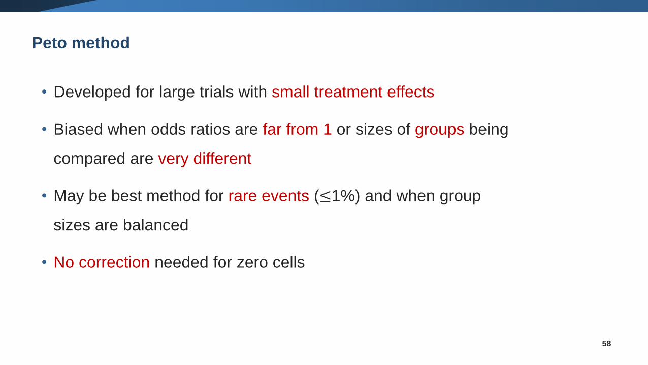
• Developed for large trials with small treatment effects
• Biased when odds ratios are far from 1 or sizes of groups being
compared are very different
• May be best method for rare events (≤1%) and when group
sizes are balanced
• No correction needed for zero cells
Peto method
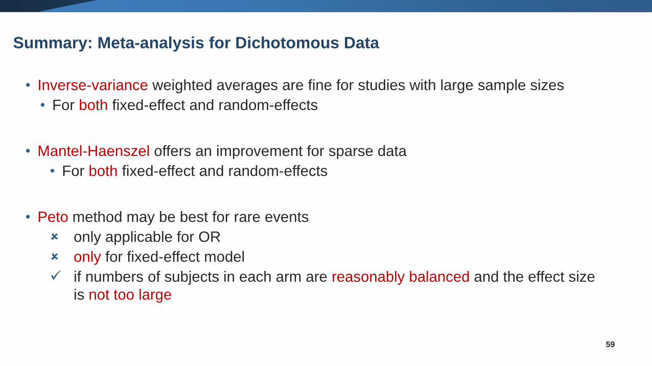
• Inverse-variance weighted averages are fine for studies with large sample sizes
• For both fixed-effect and random-effects
• Mantel-Haenszel offers an improvement for sparse data
• For both fixed-effect and random-effects
• Peto method may be best for rare events
only applicable for OR
only for fixed-effect model
✓ if numbers of subjects in each arm are reasonably balanced and the effect size
is not too large
59
Summary: Meta-analysis for Dichotomous Data
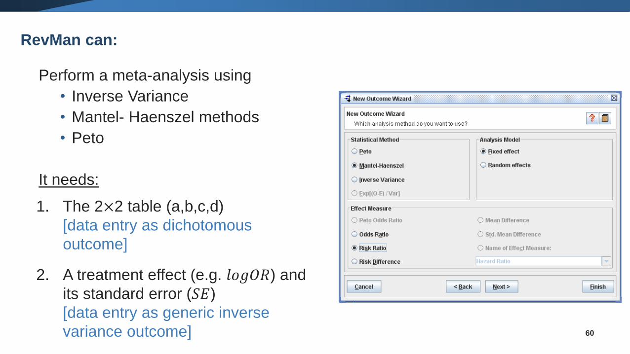
Perform a meta-analysis using
• Inverse Variance
• Mantel- Haenszel methods
• Peto
It needs:
1. The 2×2 table (a,b,c,d)
[data entry as dichotomous
outcome]
2. A treatment effect (e.g. 𝑙𝑜𝑔𝑂𝑅) and
its standard error (𝑆𝐸)
[data entry as generic inverse
variance outcome] 60
RevMan can:
Continuous data
61
62
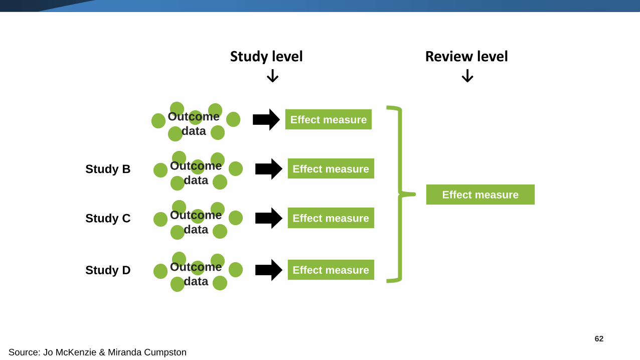
Review level↓
Effect measure
Effect measureOutcome
data
Effect measureOutcome
dataStudy B
Effect measureOutcome
dataStudy C
Effect measureOutcome
dataStudy D
Study level↓
Source: Jo McKenzie & Miranda Cumpston
63
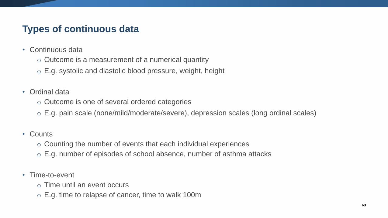
Types of continuous data
• Continuous data
o Outcome is a measurement of a numerical quantity
o E.g. systolic and diastolic blood pressure, weight, height
• Ordinal data
o Outcome is one of several ordered categories
o E.g. pain scale (none/mild/moderate/severe), depression scales (long ordinal scales)
• Counts
o Counting the number of events that each individual experiences
o E.g. number of episodes of school absence, number of asthma attacks
• Time-to-event
o Time until an event occurs
o E.g. time to relapse of cancer, time to walk 100m
64
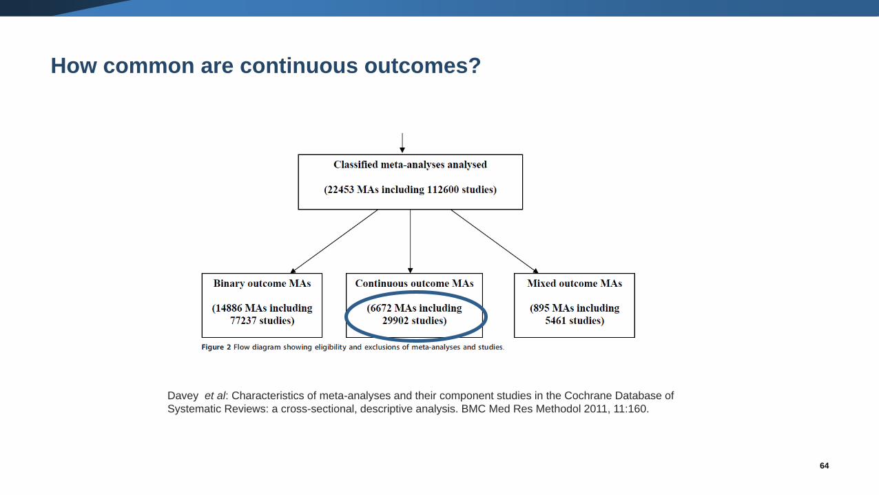
How common are continuous outcomes?
Davey et al: Characteristics of meta-analyses and their component studies in the Cochrane Database of
Systematic Reviews: a cross-sectional, descriptive analysis. BMC Med Res Methodol 2011, 11:160.
65
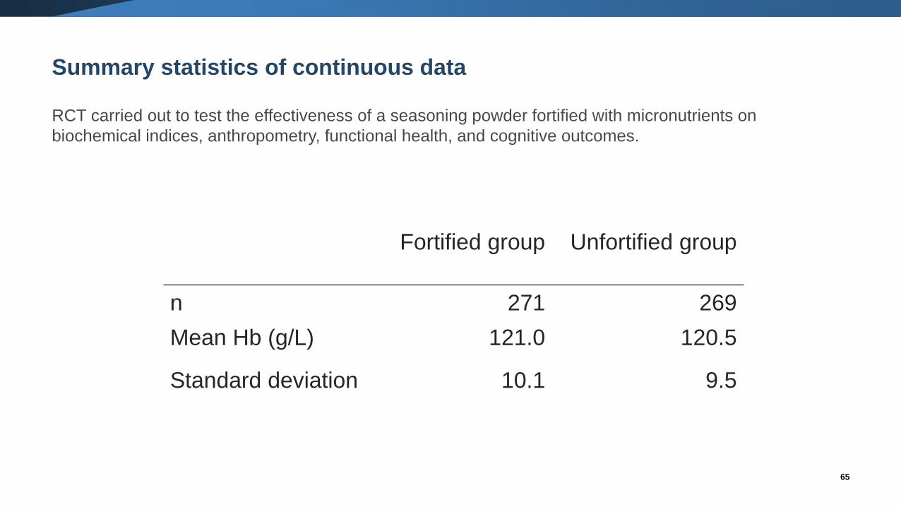
Summary statistics of continuous data
RCT carried out to test the effectiveness of a seasoning powder fortified with micronutrients on
biochemical indices, anthropometry, functional health, and cognitive outcomes.
Fortified group Unfortified group
n 271 269
Mean Hb (g/L) 121.0 120.5
Standard deviation 10.1 9.5
66
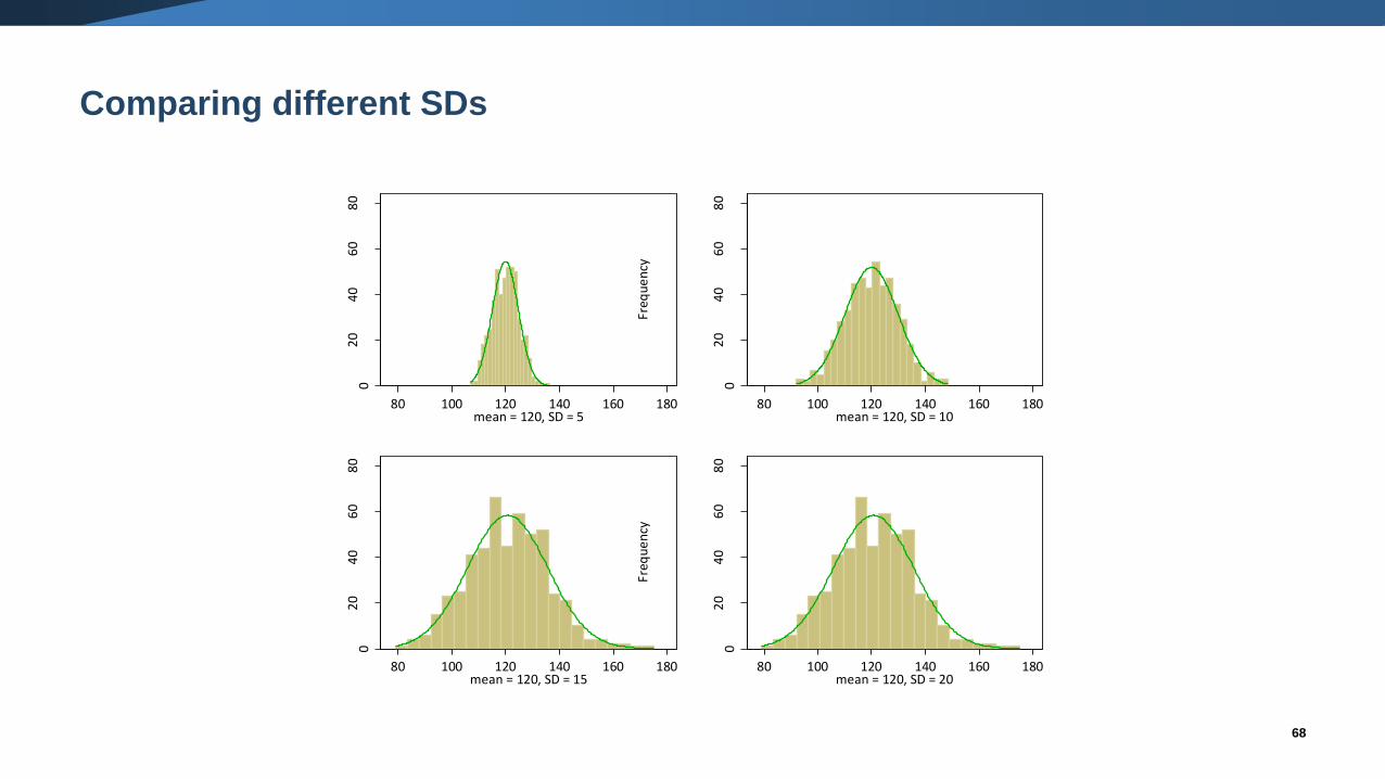
What is a standard deviation (SD)?
• A SD describes the variability in the data.
• For a particular outcome, a larger SD implies more variability than a smaller
SD.
• A measure of how far, on average, an individual’s value is from the mean.
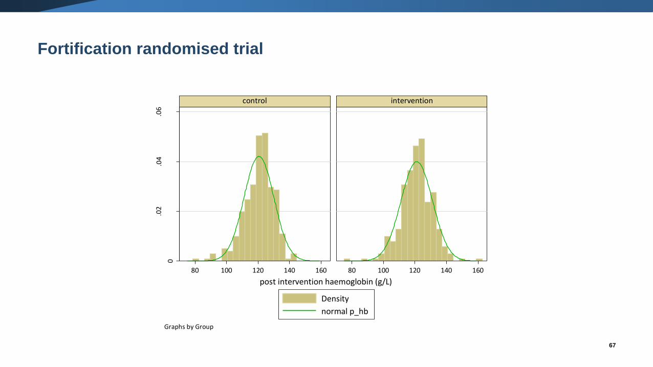
67
Fortification randomised trial
0
.02
.04
.06
80 100 120 140 160 80 100 120 140 160
control intervention
Density
normal p_hb
Den
sity
post intervention haemoglobin (g/L)
Graphs by Group
68
Comparing different SDs
02
04
06
08
0
Freq
ue
ncy
80 100 120 140 160 180mean = 120, SD = 5
02
04
06
08
0
Freq
ue
ncy
80 100 120 140 160 180mean = 120, SD = 10
02
04
06
08
0
Freq
ue
ncy
80 100 120 140 160 180mean = 120, SD = 15
02
04
06
08
0
Freq
ue
ncy
80 100 120 140 160 180mean = 120, SD = 20
69
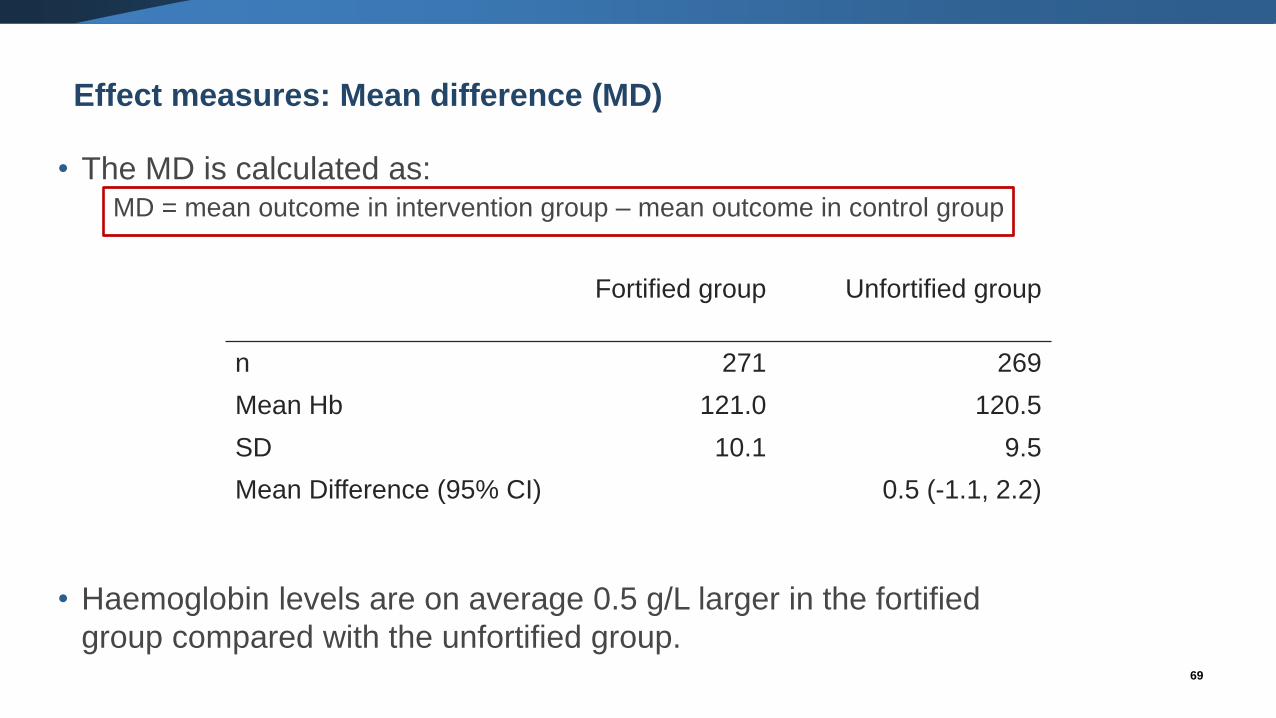
Effect measures: Mean difference (MD)
• The MD is calculated as:MD = mean outcome in intervention group – mean outcome in control group
• Haemoglobin levels are on average 0.5 g/L larger in the fortified
group compared with the unfortified group.
Fortified group Unfortified group
n 271 269
Mean Hb 121.0 120.5
SD 10.1 9.5
Mean Difference (95% CI) 0.5 (-1.1, 2.2)
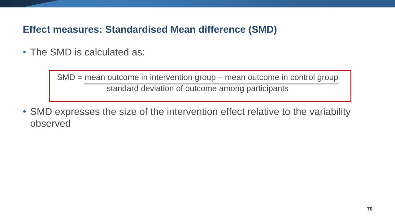
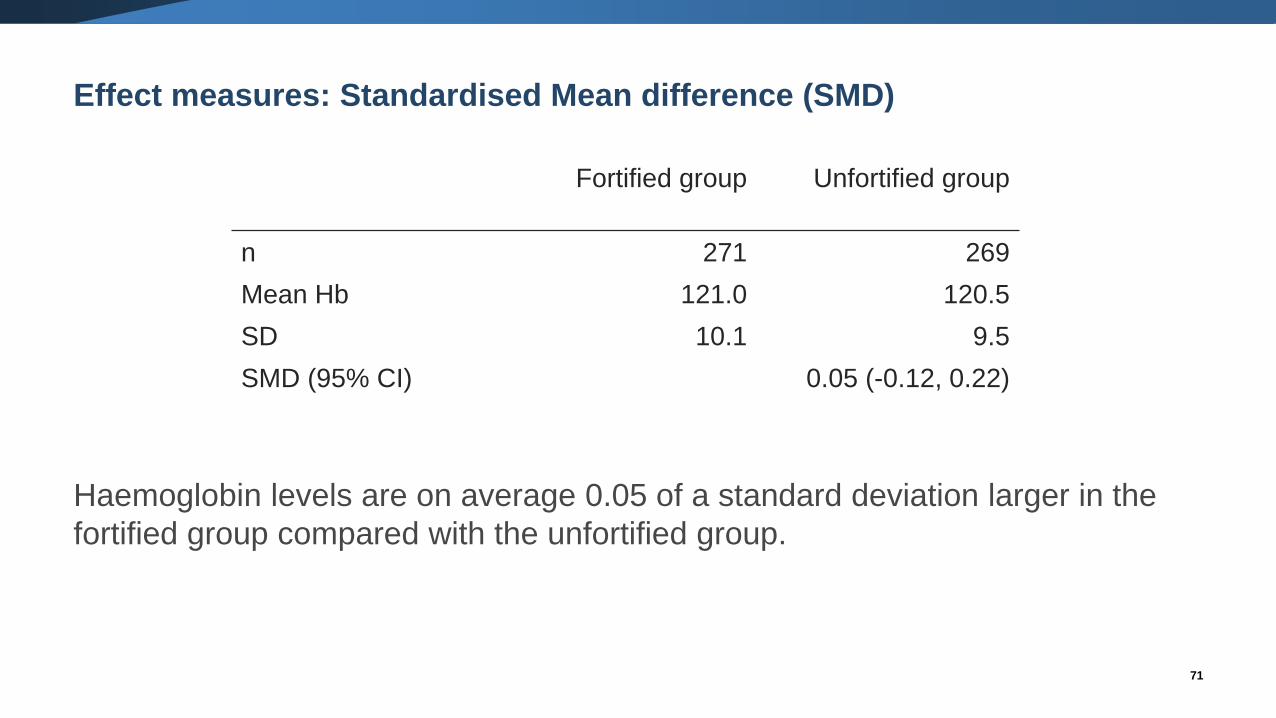
Effect measures: Standardised Mean difference (SMD)
• The SMD is calculated as:
SMD = mean outcome in intervention group – mean outcome in control group
standard deviation of outcome among participants
• SMD expresses the size of the intervention effect relative to the variability
observed
70
71
Effect measures: Standardised Mean difference (SMD)
Haemoglobin levels are on average 0.05 of a standard deviation larger in the
fortified group compared with the unfortified group.
Fortified group Unfortified group
n 271 269
Mean Hb 121.0 120.5
SD 10.1 9.5
SMD (95% CI) 0.05 (-0.12, 0.22)
72
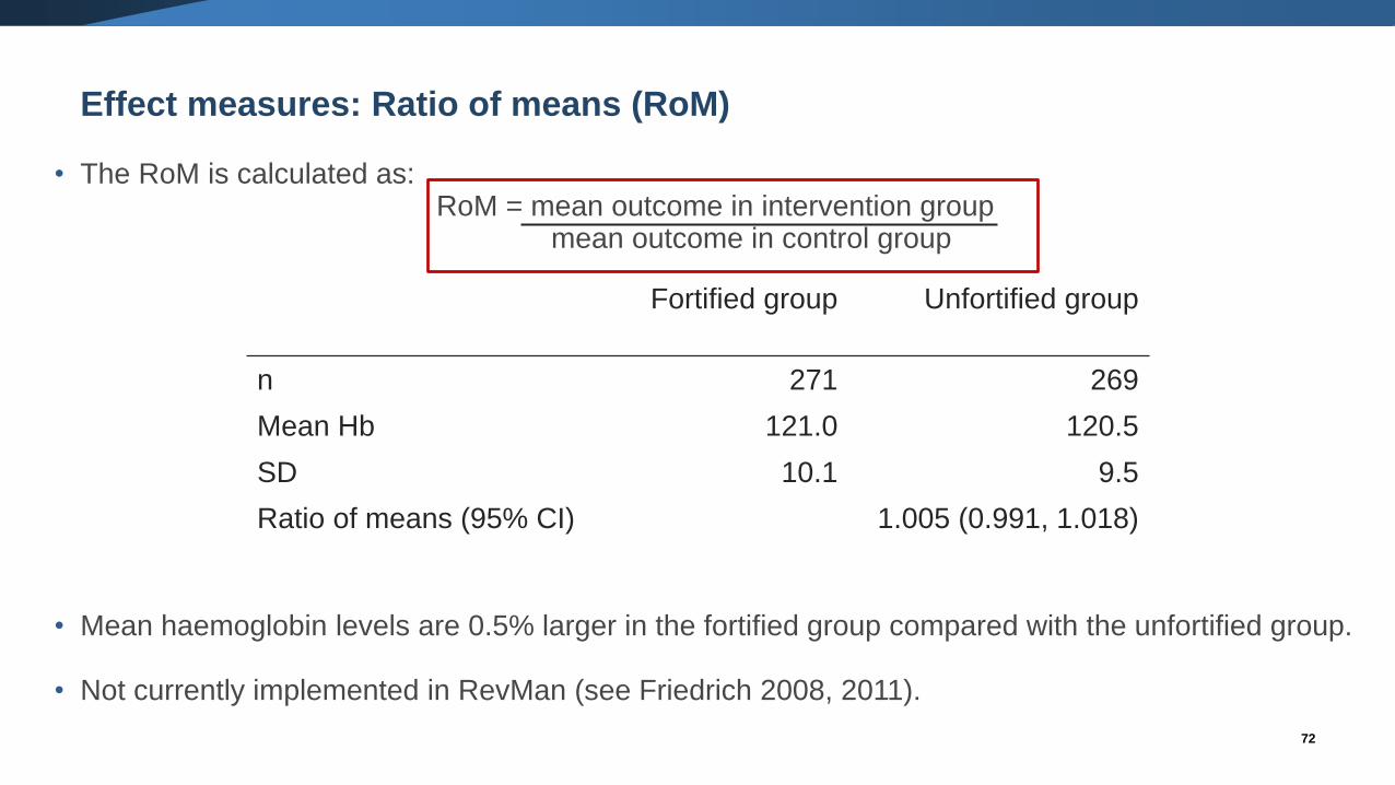
Effect measures: Ratio of means (RoM)
• The RoM is calculated as:RoM = mean outcome in intervention group
mean outcome in control group
• Mean haemoglobin levels are 0.5% larger in the fortified group compared with the unfortified group.
• Not currently implemented in RevMan (see Friedrich 2008, 2011).
Fortified group Unfortified group
n 271 269
Mean Hb 121.0 120.5
SD 10.1 9.5
Ratio of means (95% CI) 1.005 (0.991, 1.018)
73
Trial Campbell-Yeo 2010 Da Silva 2001 Rai 2016 Blank 2003
Intervention group Domperidon
e
Placebo Domperido
ne
Placebo Domperido
ne
Placebo Domperi
done
Placebo
n Stats n Stats n Stats n Stats n Stats n Stats n Stats n Stats
Baseline daily milk volume (mls)
Mean (SD or SE, as indicated) 21 184.4
(SD
167.0)
24 217.7
(SD
154.5)
7 112.8
(SD
128.7)
9 48.2
(SD
63.3)
9 120
(SE
27)
9 143
(SE
19)
Median (lower quartile, upper
quartile)
16 18.0
(12.0,
32.0)
14 21.0
(14.0,
41.0)
Follow-up daily milk volume
(mls)
Mean (SD or SE, as indicated) 21 380.2
(SD
201.6)
24 250.8
(SD
171.6)
6 183.5
(NR)
8 66.1
(NR)
9 239
(SE
35)
9 172
(SE
39)
Median (lower quartile, upper
quartile)
16 219
(116,
287)
14 102
(96,
113)
Difference in mean change
between groups (mls)
Difference (95%CI) 88.6 (95%CI 32.5 to 144.8)
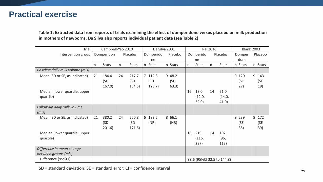
Table 1: Extracted data from reports of trials examining the effect of domperidone versus placebo on milk productionin mothers of newborns. Da Silva also reports individual patient data (see Table 2)
Practical exercise
SD = standard deviation; SE = standard error; CI = confidence interval
74
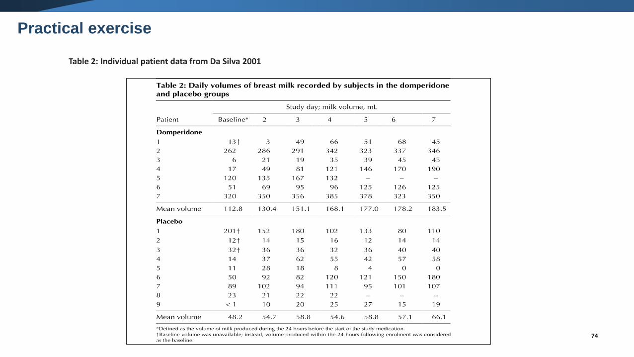
Table 2: Individual patient data from Da Silva 2001
Practical exercise
Practical exercise: Questions to consider
• What are some of the features of the data reported?
• Is there enough information provided to calculate an estimate of intervention effect for each
trial?
• What effect measure would you use?
• How would you calculate the effect estimate?
• What information might you need to calculated the standard error (or confidence interval) of
the effect estimate?
75
76
Meta-analysis (1)
• Meta-analysis is a statistical analysis of the intervention effects from several
studies leading to a quantitative summary.
• Two stages of meta-analysis:
1. An observed intervention effect is calculated for each study (e.g. MD,
SMD).
2. A pooled intervention effect estimate is calculated as a weighted
average of the intervention effects estimated in the individual studies.
Meta-analysis (2)
• A weighted average is calculated as:
Weighted average = sum of (estimate x weight)
sum of weights
• The weights reflect the amount of information that each study contributes
• The calculation of the weights differs depending on the effect measure (e.g.
MD, SMD)
• Different types of meta-analysis models can be fitted (fixed effect versus
random effects), and the weights can differ depending on the model
77
78
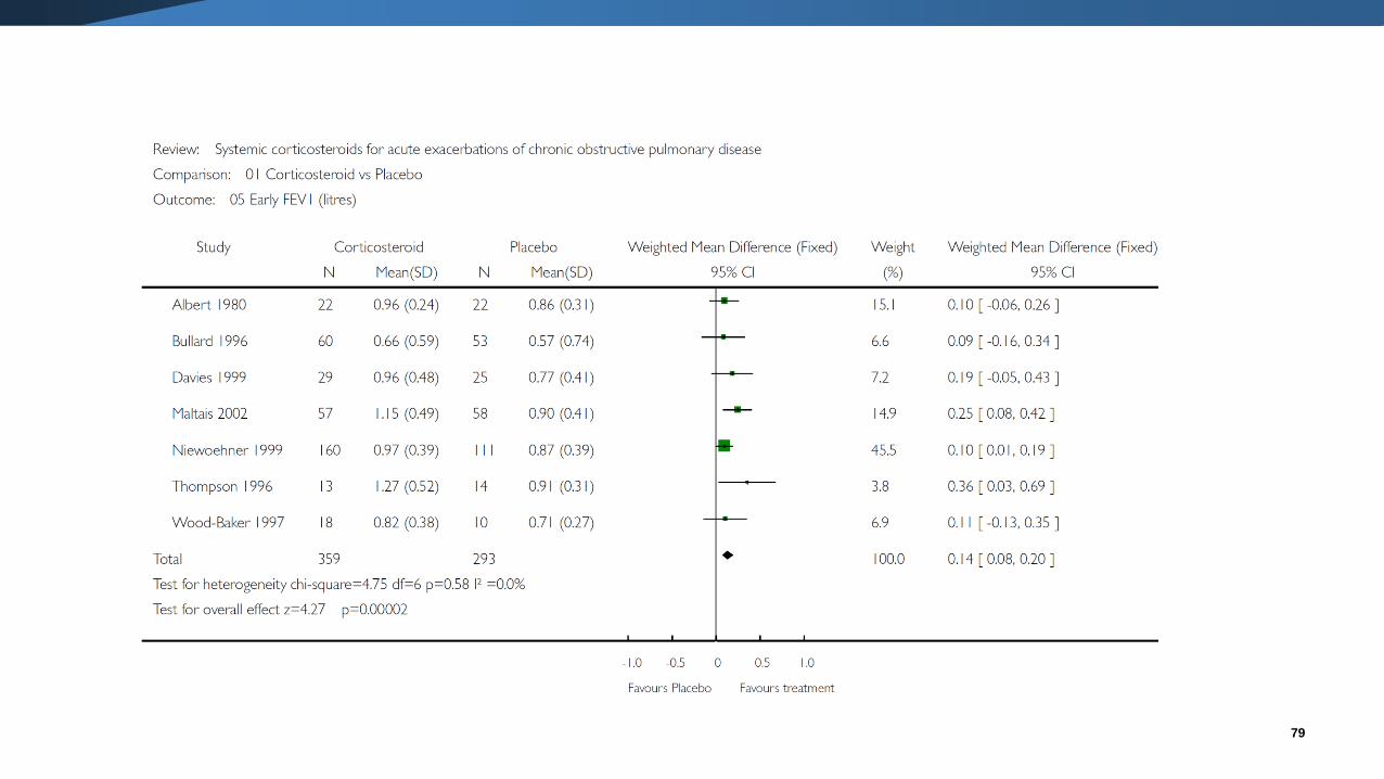
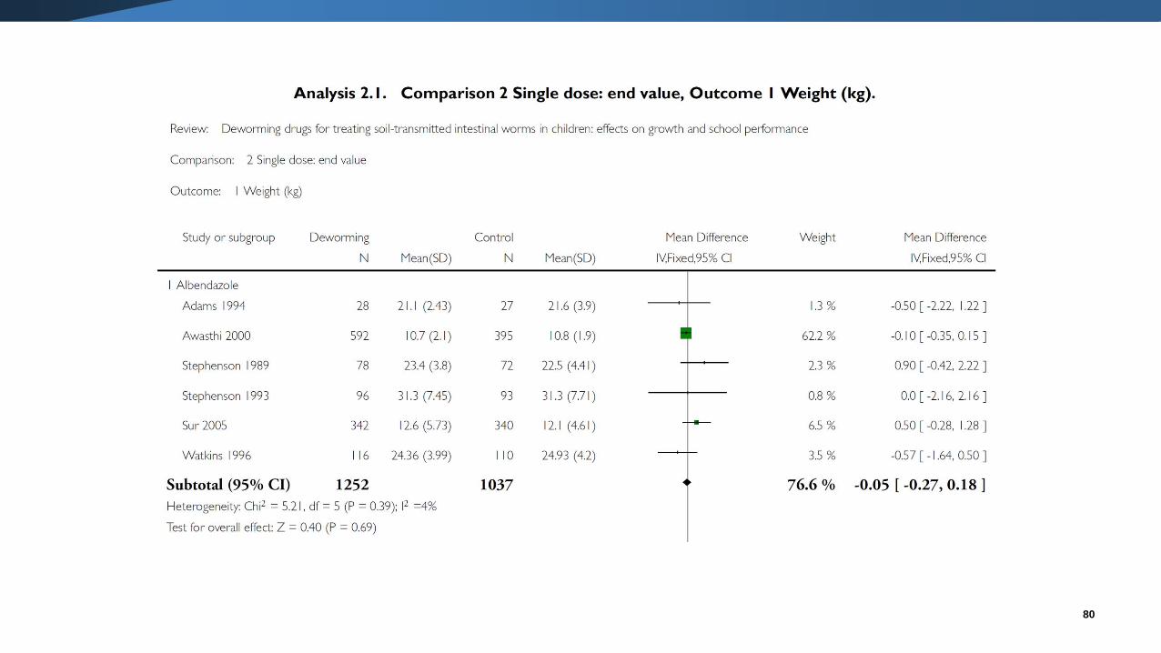
Meta-analysis: MD
• Use the mean difference when studies all report outcomes using the same
scale.
• The weighting a study receives is based on the SDs and sample size.
oFor studies of the same size, those studies with smaller SDs will be given
relatively more weight compared with studies with larger SDs.
oFor studies with the similar SDs, those studies with larger sample sizes will
be given relatively more weight compared with studies with smaller sample
sizes.
79
80
81
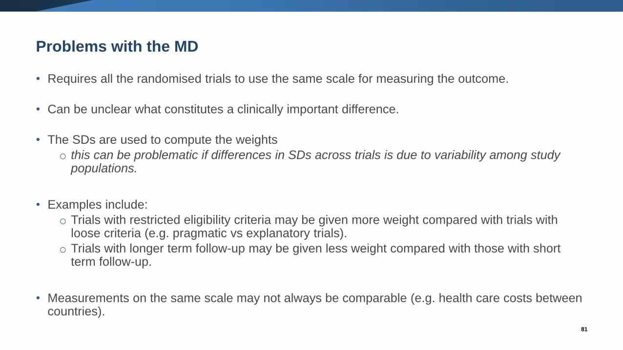
Problems with the MD
• Requires all the randomised trials to use the same scale for measuring the outcome.
• Can be unclear what constitutes a clinically important difference.
• The SDs are used to compute the weights
o this can be problematic if differences in SDs across trials is due to variability among study populations.
• Examples include:
o Trials with restricted eligibility criteria may be given more weight compared with trials with loose criteria (e.g. pragmatic vs explanatory trials).
o Trials with longer term follow-up may be given less weight compared with those with short term follow-up.
• Measurements on the same scale may not always be comparable (e.g. health care costs between countries).
82
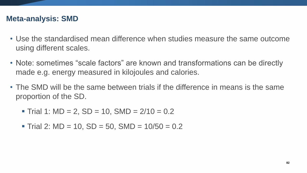
Meta-analysis: SMD
• Use the standardised mean difference when studies measure the same outcome
using different scales.
• Note: sometimes “scale factors” are known and transformations can be directly
made e.g. energy measured in kilojoules and calories.
• The SMD will be the same between trials if the difference in means is the same
proportion of the SD.
▪ Trial 1: MD = 2, SD = 10, SMD = 2/10 = 0.2
▪ Trial 2: MD = 10, SD = 50, SMD = 10/50 = 0.2
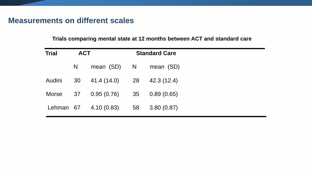
Trials comparing mental state at 12 months between ACT and standard care
ACT Standard Care
N mean (SD) N mean (SD)
30 41.4 (14.0) 28 42.3 (12.4)
37 0.95 (0.76) 35 0.89 (0.65)
67 4.10 (0.83) 58 3.80 (0.87)
Audini
Morse
Lehman
Trial
Measurements on different scales
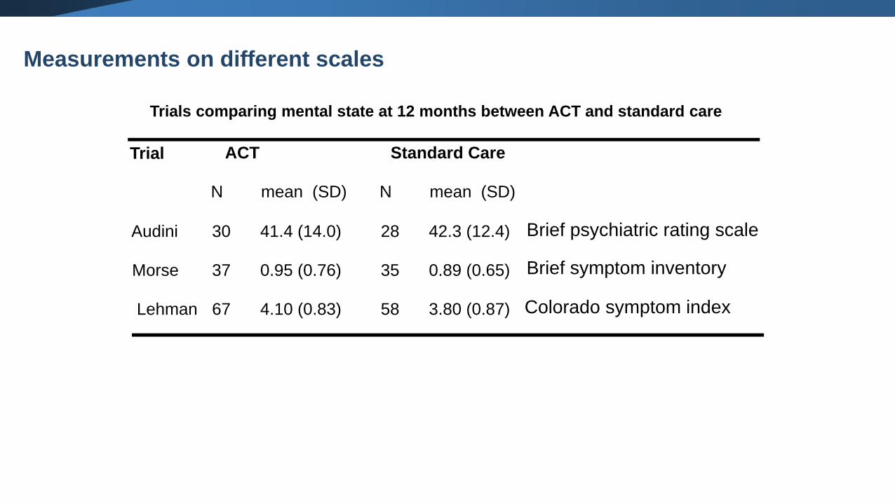
Trials comparing mental state at 12 months between ACT and standard care
ACT Standard Care
N mean (SD) N mean (SD)
30 41.4 (14.0) 28 42.3 (12.4)
37 0.95 (0.76) 35 0.89 (0.65)
67 4.10 (0.83) 58 3.80 (0.87)
Audini
Morse
Lehman
Trial
Brief psychiatric rating scale
Brief symptom inventory
Colorado symptom index
Measurements on different scales
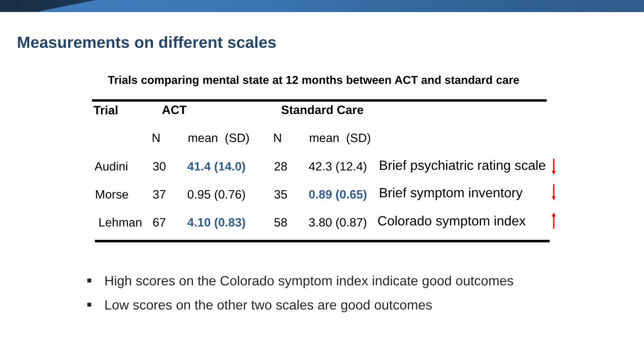
Trials comparing mental state at 12 months between ACT and standard care
ACT Standard Care
N mean (SD) N mean (SD)
30 41.4 (14.0) 28 42.3 (12.4)
37 0.95 (0.76) 35 0.89 (0.65)
67 4.10 (0.83) 58 3.80 (0.87)
Audini
Morse
Lehman
Trial
Brief psychiatric rating scale
Brief symptom inventory
Colorado symptom index
▪ High scores on the Colorado symptom index indicate good outcomes
▪ Low scores on the other two scales are good outcomes
Measurements on different scales
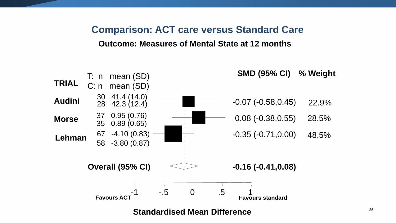
Standardised Mean Difference
Morse
Lehman
TRIAL
Comparison: ACT care versus Standard Care
Outcome: Measures of Mental State at 12 months
-1 -.5 0 .5 1
% WeightSMD (95% CI)
-0.07 (-0.58,0.45)Audini30 41.4 (14.0)28 42.3 (12.4) 22.9%
0.08 (-0.38,0.55)37 0.95 (0.76)35 0.89 (0.65)
28.5%
-0.35 (-0.71,0.00)67 -4.10 (0.83)
58 -3.80 (0.87)48.5%
-0.16 (-0.41,0.08)Overall (95% CI)
T: n mean (SD)
C: n mean (SD)
Favours ACT Favours standard
86
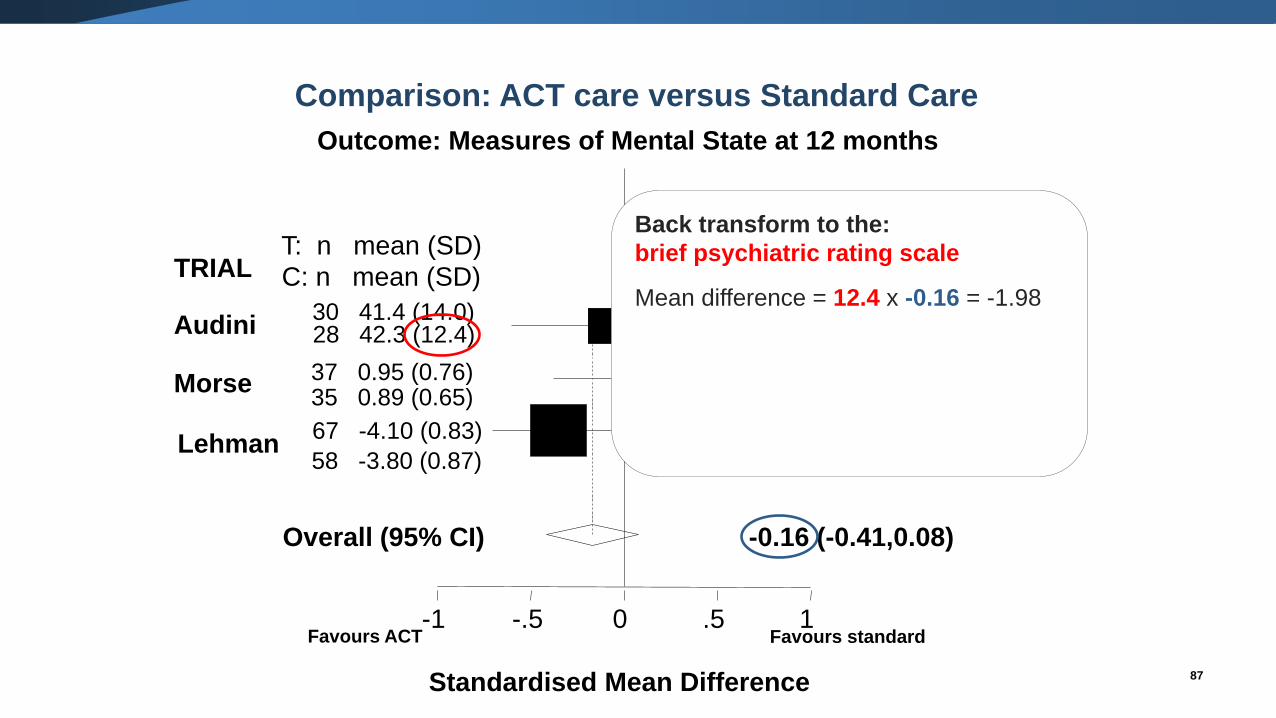
Standardised Mean Difference
Morse
Lehman
TRIAL
-1 -.5 0 .5 1
% WeightSMD (95% CI)
-0.07 (-0.58,0.45)Audini30 41.4 (14.0)28 42.3 (12.4) 22.9%
0.08 (-0.38,0.55)37 0.95 (0.76)35 0.89 (0.65)
28.5%
-0.35 (-0.71,0.00)67 -4.10 (0.83)
58 -3.80 (0.87)48.5%
-0.16 (-0.41,0.08)Overall (95% CI)
T: n mean (SD)
C: n mean (SD)
Favours ACT Favours standard
87
Back transform to the:
brief psychiatric rating scale
Mean difference = 12.4 x -0.16 = -1.98
Comparison: ACT care versus Standard Care
Outcome: Measures of Mental State at 12 months

Standardised Mean Difference
Morse
Lehman
TRIAL
-1 -.5 0 .5 1
% WeightSMD (95% CI)
-0.07 (-0.58,0.45)Audini30 41.4 (14.0)28 42.3 (12.4) 22.9%
0.08 (-0.38,0.55)37 0.95 (0.76)35 0.89 (0.65)
28.5%
-0.35 (-0.71,0.00)67 -4.10 (0.83)
58 -3.80 (0.87)48.5%
-0.16 (-0.41,0.08)Overall (95% CI)
T: n mean (SD)
C: n mean (SD)
Favours ACT Favours standard
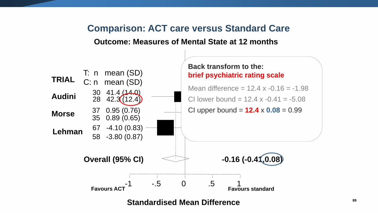
88
Back transform to the:
brief psychiatric rating scale
Mean difference = 12.4 x -0.16 = -1.98
CI lower bound = 12.4 x -0.41 = -5.08
Comparison: ACT care versus Standard Care
Outcome: Measures of Mental State at 12 months
Standardised Mean Difference
Morse
Lehman
TRIAL
-1 -.5 0 .5 1
% WeightSMD (95% CI)
-0.07 (-0.58,0.45)Audini30 41.4 (14.0)28 42.3 (12.4) 22.9%
0.08 (-0.38,0.55)37 0.95 (0.76)35 0.89 (0.65)
28.5%
-0.35 (-0.71,0.00)67 -4.10 (0.83)
58 -3.80 (0.87)48.5%
-0.16 (-0.41,0.08)Overall (95% CI)
T: n mean (SD)
C: n mean (SD)
Favours ACT Favours standard
89
Back transform to the:
brief psychiatric rating scale
Mean difference = 12.4 x -0.16 = -1.98
CI lower bound = 12.4 x -0.41 = -5.08
CI upper bound = 12.4 x 0.08 = 0.99
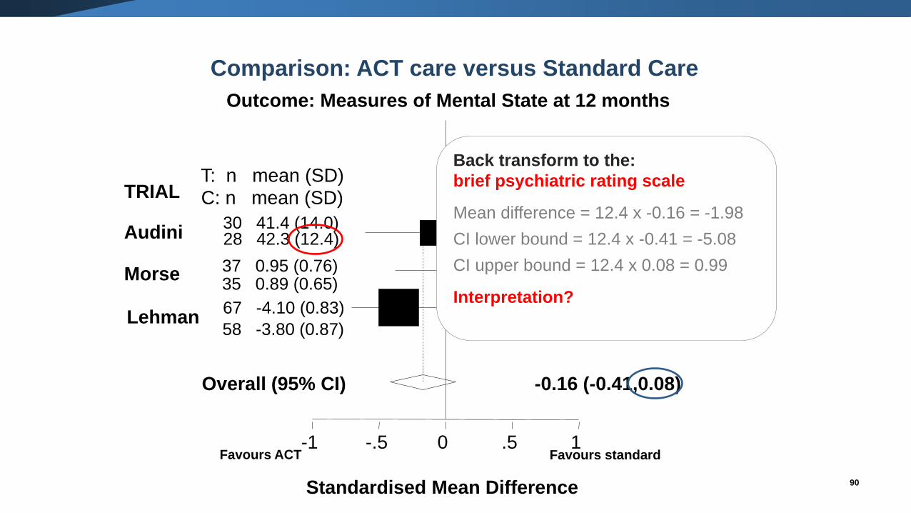
Comparison: ACT care versus Standard Care
Outcome: Measures of Mental State at 12 months
Standardised Mean Difference
Morse
Lehman
TRIAL
-1 -.5 0 .5 1
% WeightSMD (95% CI)
-0.07 (-0.58,0.45)Audini30 41.4 (14.0)28 42.3 (12.4) 22.9%
0.08 (-0.38,0.55)37 0.95 (0.76)35 0.89 (0.65)
28.5%
-0.35 (-0.71,0.00)67 -4.10 (0.83)
58 -3.80 (0.87)48.5%
-0.16 (-0.41,0.08)Overall (95% CI)
T: n mean (SD)
C: n mean (SD)
Favours ACT Favours standard
90
Back transform to the:
brief psychiatric rating scale
Mean difference = 12.4 x -0.16 = -1.98
CI lower bound = 12.4 x -0.41 = -5.08
CI upper bound = 12.4 x 0.08 = 0.99
Interpretation?
Comparison: ACT care versus Standard Care
Outcome: Measures of Mental State at 12 months
Standardised Mean Difference
Morse
Lehman
TRIAL
-1 -.5 0 .5 1
% WeightSMD (95% CI)
-0.07 (-0.58,0.45)Audini30 41.4 (14.0)28 42.3 (12.4) 22.9%
0.08 (-0.38,0.55)37 0.95 (0.76)35 0.89 (0.65)
28.5%
-0.35 (-0.71,0.00)67 -4.10 (0.83)
58 -3.80 (0.87)48.5%
-0.16 (-0.41,0.08)Overall (95% CI)
T: n mean (SD)
C: n mean (SD)
Favours ACT Favours standard
91
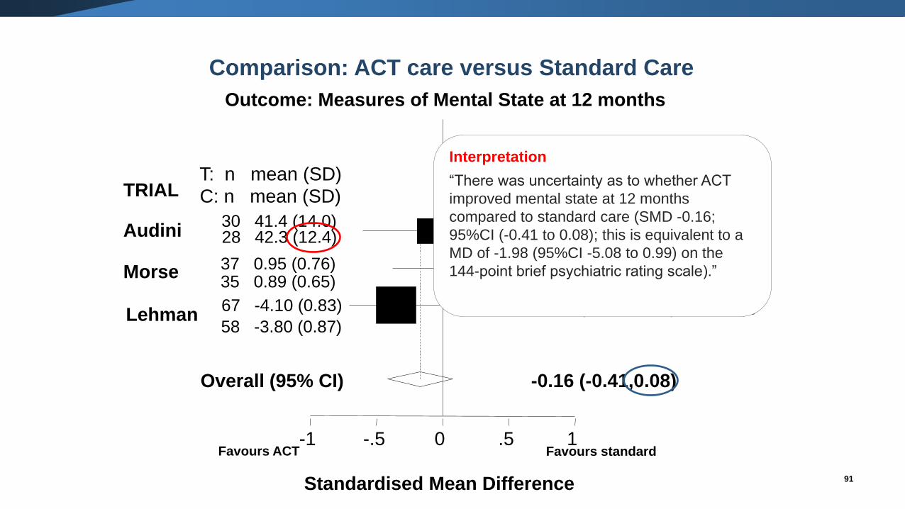
Interpretation
“There was uncertainty as to whether ACT
improved mental state at 12 months
compared to standard care (SMD -0.16;
95%CI (-0.41 to 0.08); this is equivalent to a
MD of -1.98 (95%CI -5.08 to 0.99) on the
144-point brief psychiatric rating scale).”
Comparison: ACT care versus Standard Care
Outcome: Measures of Mental State at 12 months
92
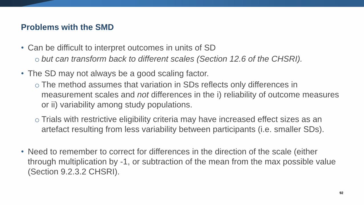
Problems with the SMD
• Can be difficult to interpret outcomes in units of SD
o but can transform back to different scales (Section 12.6 of the CHSRI).
• The SD may not always be a good scaling factor.
o The method assumes that variation in SDs reflects only differences in
measurement scales and not differences in the i) reliability of outcome measures
or ii) variability among study populations.
o Trials with restrictive eligibility criteria may have increased effect sizes as an
artefact resulting from less variability between participants (i.e. smaller SDs).
• Need to remember to correct for differences in the direction of the scale (either
through multiplication by -1, or subtraction of the mean from the max possible value
(Section 9.2.3.2 CHSRI).
93
Data extraction
• Chapter 7 (Section 7.7.3) CHSRI.
• Two ways of entering continuous data in RevMan:
o Entering means, SDs, and number of participants for the intervention and control groups.
o Entering the intervention effect and its standard error.
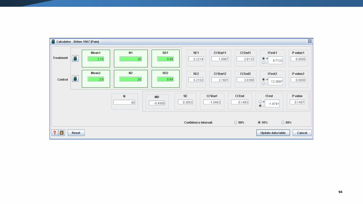
• These methods cannot be used in combination. But …
o RevMan 5.1 has a calculator which facilitates transformation between various statistics.
94
Data extraction
• Be careful to extract all reported statistics.
• While SDs may not be directly reported, they can be computed from:
o standard errors
o confidence intervals
o t-tests
o p-values from t and z tests.
• May need to search tables, text, and graphs for SDs.
• It may be the case that the SD needs to be imputed for some of the trials.
o Contact the publication authors.
o Use information on SDs from other trials.
o Carry out sensitivity analyses investigating the effect of imputation.
o Be careful to note in the review which SDs are imputed.
o See Wiebe 2006 for options.
95
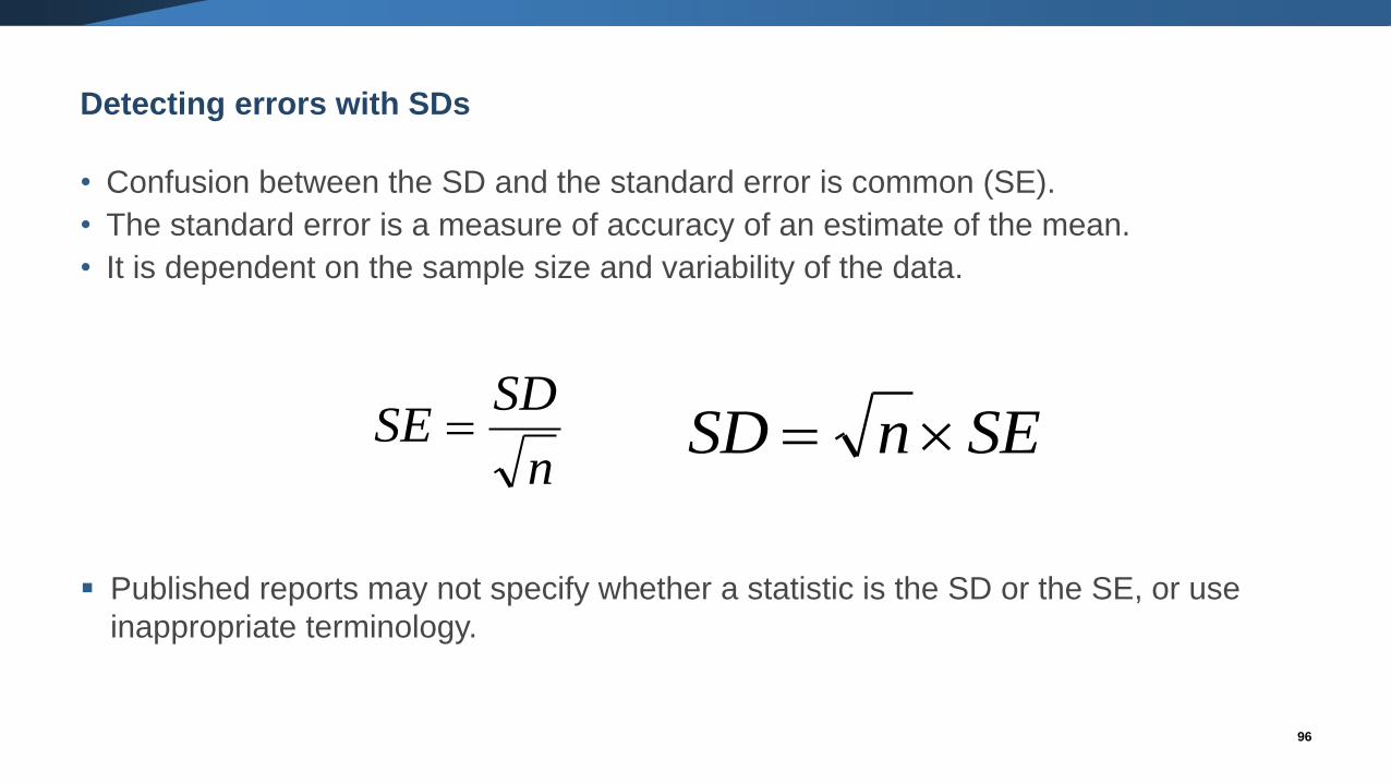
Detecting errors with SDs
• Confusion between the SD and the standard error is common (SE).
• The standard error is a measure of accuracy of an estimate of the mean.
• It is dependent on the sample size and variability of the data.
▪ Published reports may not specify whether a statistic is the SD or the SE, or use
inappropriate terminology.
96
n
SDSE = SEnSD =
Study or Subgroup
1.1.1 600 mcg
Hong Kong 2001
Nigeria 2003
Turkey 2003
WHO 1999
WHO 2001
Subtotal (95% CI)
Heterogeneity: Chi² = 113.57, df = 4 (P < 0.00001); I² = 96%
Test for overall effect: Z = 6.69 (P < 0.00001)
Total (95% CI)
Heterogeneity: Chi² = 113.57, df = 4 (P < 0.00001); I² = 96%
Test for overall effect: Z = 6.69 (P < 0.00001)
Test for subgroup differences: Not applicable
Mean
296
341
328
340.9
332.8
SD
160
19.3
152
295.08
274.6
Total
1026
247
388
199
9213
11073
11073
Mean
254
339
312
352.6
289.7
SD
157
18.9
176
309.59
262.1
Total
1032
249
384
200
9227
11092
11092
Weight
4.7%
78.6%
1.6%
0.3%
14.8%
100.0%
100.0%
IV, Fixed, 95% CI
42.00 [28.30, 55.70]
2.00 [-1.36, 5.36]
16.00 [-7.21, 39.21]
-11.70 [-71.04, 47.64]
43.10 [35.35, 50.85]
10.17 [7.19, 13.15]
10.17 [7.19, 13.15]
Oral misoprostol Injectable uterotonics Mean Difference Mean Difference
IV, Fixed, 95% CI
-100 -50 0 50 100
Favours oral misoprostol Favours Injectable uterotonics
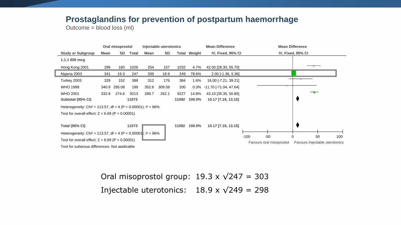
Prostaglandins for prevention of postpartum haemorrhageOutcome = blood loss (ml)
Oral misoprostol group: 19.3 x √247 = 303
Injectable uterotonics: 18.9 x √249 = 298
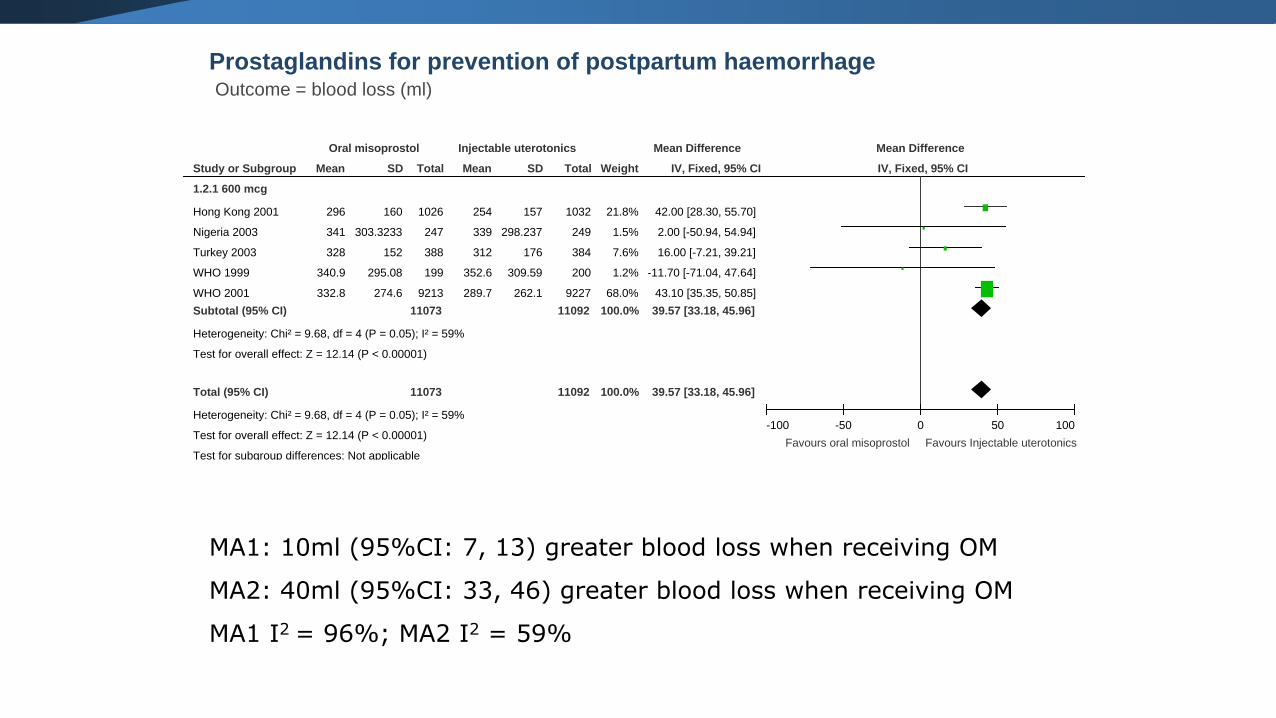
Prostaglandins for prevention of postpartum haemorrhageOutcome = blood loss (ml)
Study or Subgroup
1.2.1 600 mcg
Hong Kong 2001
Nigeria 2003
Turkey 2003
WHO 1999
WHO 2001
Subtotal (95% CI)
Heterogeneity: Chi² = 9.68, df = 4 (P = 0.05); I² = 59%
Test for overall effect: Z = 12.14 (P < 0.00001)
Total (95% CI)
Heterogeneity: Chi² = 9.68, df = 4 (P = 0.05); I² = 59%
Test for overall effect: Z = 12.14 (P < 0.00001)
Test for subgroup differences: Not applicable
Mean
296
341
328
340.9
332.8
SD
160
303.3233
152
295.08
274.6
Total
1026
247
388
199
9213
11073
11073
Mean
254
339
312
352.6
289.7
SD
157
298.237
176
309.59
262.1
Total
1032
249
384
200
9227
11092
11092
Weight
21.8%
1.5%
7.6%
1.2%
68.0%
100.0%
100.0%
IV, Fixed, 95% CI
42.00 [28.30, 55.70]
2.00 [-50.94, 54.94]
16.00 [-7.21, 39.21]
-11.70 [-71.04, 47.64]
43.10 [35.35, 50.85]
39.57 [33.18, 45.96]
39.57 [33.18, 45.96]
Oral misoprostol Injectable uterotonics Mean Difference Mean Difference
IV, Fixed, 95% CI
-100 -50 0 50 100
Favours oral misoprostol Favours Injectable uterotonics
MA1: 10ml (95%CI: 7, 13) greater blood loss when receiving OM
MA2: 40ml (95%CI: 33, 46) greater blood loss when receiving OM
MA1 I2 = 96%; MA2 I2 = 59%
99
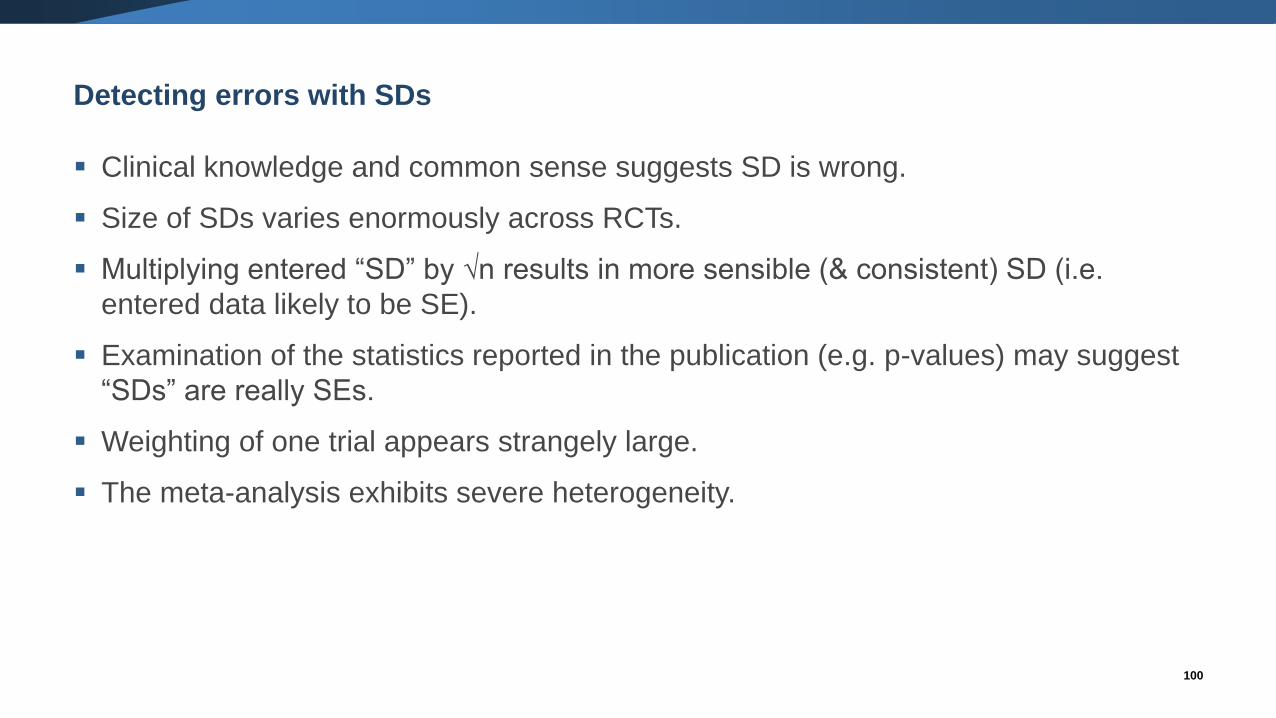
Detecting errors with SDs
▪ Clinical knowledge and common sense suggests SD is wrong.
▪ Size of SDs varies enormously across RCTs.
▪ Multiplying entered “SD” by √n results in more sensible (& consistent) SD (i.e.
entered data likely to be SE).
▪ Examination of the statistics reported in the publication (e.g. p-values) may suggest
“SDs” are really SEs.
▪ Weighting of one trial appears strangely large.
▪ The meta-analysis exhibits severe heterogeneity.
100
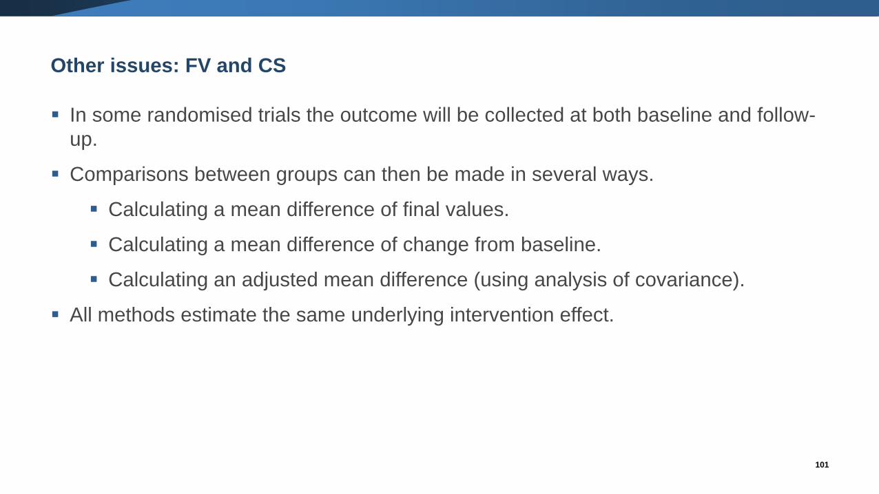
Other issues: FV and CS
▪ In some randomised trials the outcome will be collected at both baseline and follow-
up.
▪ Comparisons between groups can then be made in several ways.
▪ Calculating a mean difference of final values.
▪ Calculating a mean difference of change from baseline.
▪ Calculating an adjusted mean difference (using analysis of covariance).
▪ All methods estimate the same underlying intervention effect.
101
102
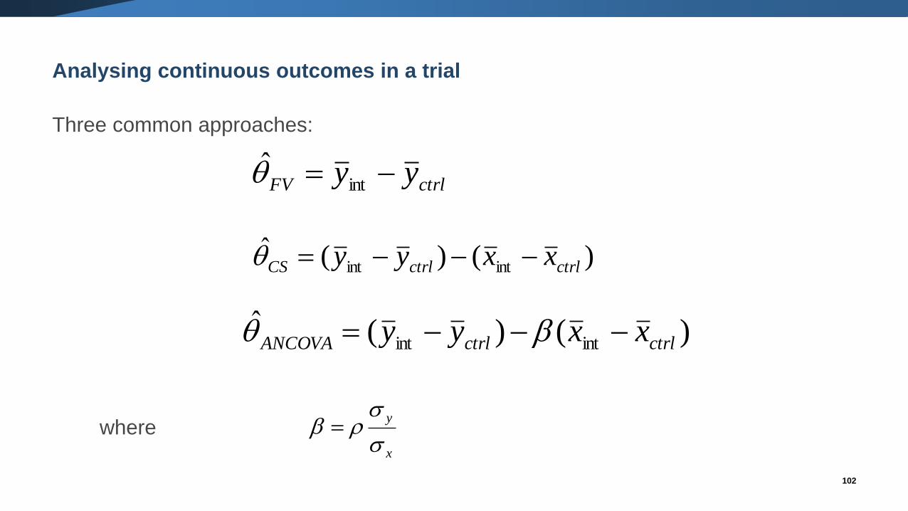
Analysing continuous outcomes in a trial
Three common approaches:
where
ctrlFV yy −= int̂
)()(ˆintint ctrlctrlCS xxyy −−−=
)()(ˆintint ctrlctrlANCOVA xxyy −−−=
x
y
=
Other issues
103
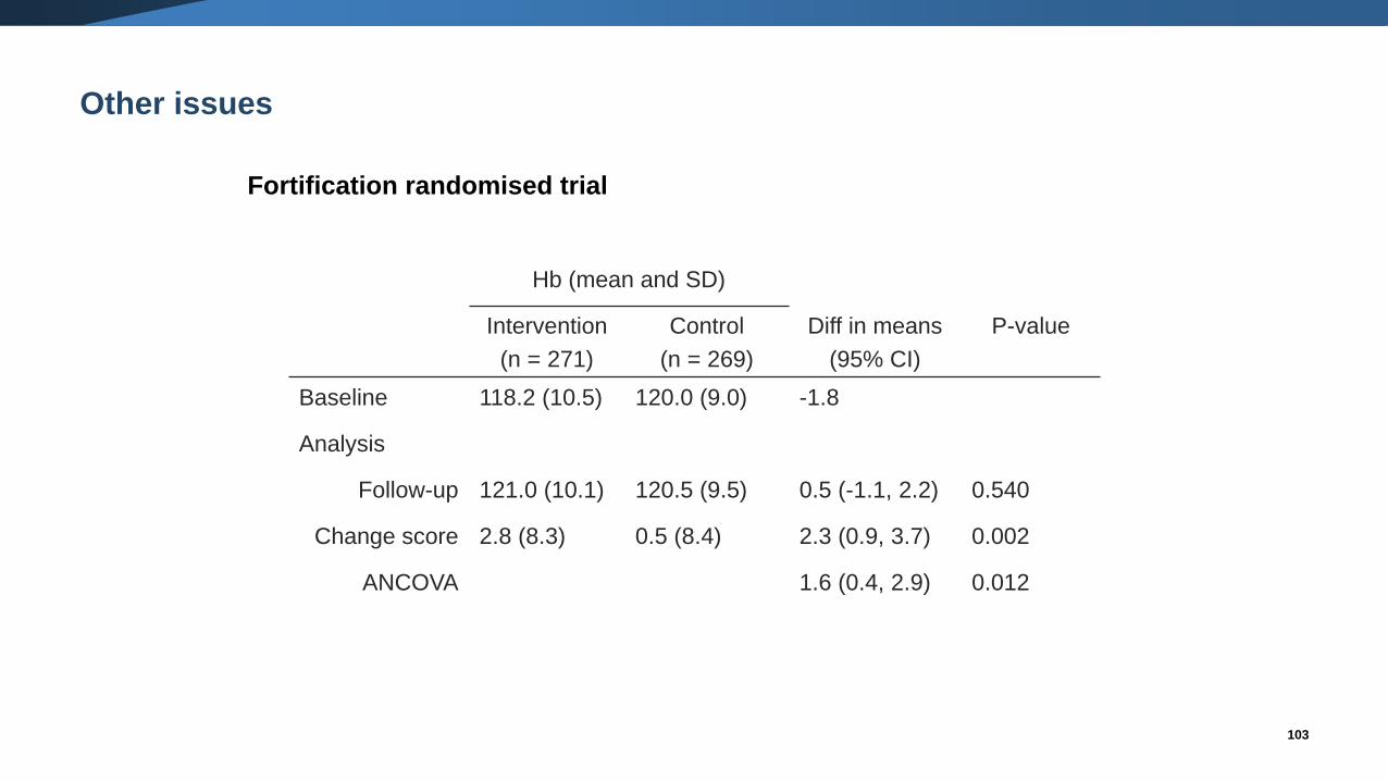
Fortification randomised trial
Hb (mean and SD)
Intervention
(n = 271)
Control
(n = 269)
Diff in means
(95% CI)
P-value
Baseline 118.2 (10.5) 120.0 (9.0) -1.8
Analysis
Follow-up 121.0 (10.1) 120.5 (9.5) 0.5 (-1.1, 2.2) 0.540
Change score 2.8 (8.3) 0.5 (8.4) 2.3 (0.9, 3.7) 0.002
ANCOVA 1.6 (0.4, 2.9) 0.012
Other issues: FV and CS
▪ In some randomised trials the outcome will be collected at both baseline and follow-up.
▪ Comparisons between groups can then be made in several ways.
▪ Calculating a mean difference of final values.
▪ Calculating a mean difference of change from baseline.
▪ Calculating an adjusted mean difference (using analysis of covariance).
▪ All methods estimate the same underlying intervention effect.
▪ Therefore, we can combine the results from the different methods in one meta-analysis.
▪ The precision of the estimates will differ, depending on the correlation between the
baseline measure of the outcome and the outcome.
▪ Can not use a mixture of the methods when using the SMD.
104
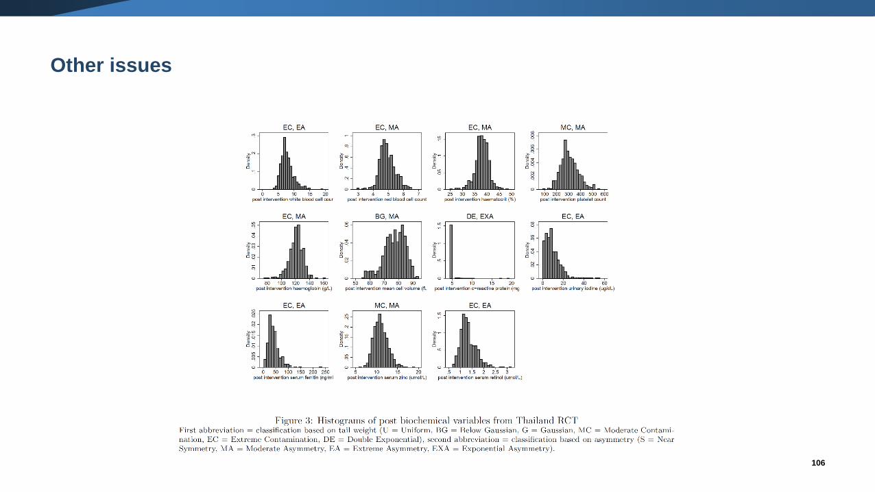
Other issues: non-normality
▪ Standard meta-analytic methods assume normality in the distribution of the means.
▪ Many outcomes are not normally distributed.
105
106
Other issues
Other issues: non-normality
▪ Standard meta-analytic methods assume normality in the distribution of the means.
▪ Many outcomes are not normally distributed.
▪ Indications of skew include:
▪ Geometric means, medians, interquartile ranges reported.
▪ Large SD compared with the mean.
▪ (mean – lowest possible score)/SD < 2 indicates skew
▪ (highest possible score – mean)/SD < 2 indicates skew
▪ Methods are available to estimate parametric statistics (mean, SD) from non-parametric
statistics (median, inter-quartile, range) (e.g. Hozo 2005; Wan 2014, Luo 2016), Weir
2018)
107
Other issues: non-normality
▪ In large trials, skewed distributions are not likely to be problematic.
▪ In small trials, may conduct the meta-analysis on the log-transformed scale (if this scale
is believed to be less skewed) (Higgins 2008)
▪ Seek statistical support.
108
The Cochrane Collaboration
• CENTRAL provides the most comprehensive database of trials
• Provides a free software for systematic reviews and meta-analyses (Review Manager; RevMan)
– For a practical on RevMan see: https://www.youtube.com/watch?v=I6gqY5GkwMs
• See also the Cochrane Handbook (http://community.cochrane.org/handbook) that describes in
detail the process of preparing and maintaining Cochrane systematic reviews on the effects of
healthcare interventions.
o For video about systematic reviews, also visit: http://www.cochrane.org/what-is-cochrane-
evidence
109
www.cochrane.org

• Cochrane Handbook for Systematic Reviews of Interventions
-Higgins and Green (eds); Wiley 2008, updated online
• RevMan Tutorial and User Guide
-http://tech.cochrane.org/revman/documentation
• Introduction to Meta-analysis
-Borenstein, Hedge, Higgins and Rothwell; Wiley 2009
• Meta-Analysis of Controlled Clinical Trials
-Whitehead; Wiley 2002
• Cochrane online training material, available at
http://training.cochrane.org/sites/training.cochrane.org/files/uploads/satms/public/english/10_Introduction_to_
meta-analysis_1_1_Eng/story.html
• Handbook of Research Synthesis and Meta-analysis
-Cooper, Hedges and Valentine; Sage 2009
110
Resources
• Friedrich JO, Adhikari NK, Beyene J: The ratio of means method as an alternative to mean differences for analyzing continuous outcome variables in meta-analysis: a simulation study. BMC Med Res Methodol 2008, 8:32.
• Friedrich JO, Adhikari NKJ, Beyene J: Ratio of means for analyzing continuous outcomes in meta-analysis performed as well as mean difference methods. Journal of Clinical Epidemiology 2011, 64:556-564.
• Higgins JP, White IR, Anzures-Cabrera J: Meta-analysis of skewed data: Combining results reported on log-transformed or raw scales. Stat Med 2008.
• Hozo SP, Djulbegovic B, Hozo I: Estimating the mean and variance from the median, range, and the size of a sample. BMC Med Res Methodol 2005, 5(1):13.
• Luo D, Wan X, Liu J, Tong T: Optimally estimating the sample mean from the sample size, median, mid-range, and/or mid-quartile range. Stat Methods Med Res 2016.
• Wan X, Wang W, Liu J, Tong T: Estimating the sample mean and standard deviation from the sample size, median, range and/or interquartile range. BMC Medical Research Methodology 2014, 14(1):135.
• Weir CJ, Butcher I, Assi V, Lewis SC, Murray GD, Langhorne P, et al. Dealing with missing standard deviation and mean values in meta-analysis of continuous outcomes: a systematic review. BMC Medical Research Methodology. 2018;18(1):25.
• Wiebe N, Vandermeer B, Platt RW, Klassen TP, Moher D, Barrowman NJ: A systematic review identifies a lack of standardization in methods for handling missing variance data. J Clin Epidemiol 2006, 59:342-353.
111
Resources

Thank you for your attention!
Questions?
112